d-scholarship.pitt.edud-scholarship.pitt.edu/28595/1/zakerzadeh_etdpitt2016.pdf · in this work, we...

A COMPUTATIONAL MODEL FOR FLUID-POROUS STRUCTURE INTERACTION

by

Rana Zakerzadeh

B.Sc. in Biomedical Engineering, Tehran Polytechnic, 2009

M.Sc. in Biomedical Engineering, Tehran Polytechnic, 2011

Submitted to the Graduate Faculty of

Swanson School of Engineering in partial fulfillment

of the requirements for the degree of

Doctor of Philosophy

University of Pittsburgh

2016

ii

UNIVERSITY OF PITTSBURGH

SWANSON SCHOOL OF ENGINEERING

This dissertation was presented

by

Rana Zakerzadeh

It was defended on

July 26, 2016

and approved by

Peyman Givi, Ph.D. Distinguished Professor and James T. MacLeod Professor, Department of

Mechanical Engineering & Materials Science

Spandan Maiti, Ph.D., Assistant Professor, Department of Bioengineering

Anne Robertson, Ph.D., William Kepler Whiteford Professor, Department of Mechanical

Engineering & Materials Science

Dissertation Director: Paolo Zunino, Ph.D., Assistant Professor, Department of Mechanical

Engineering & Materials Science

iii

Copyright © by Rana Zakerzadeh

2016

iv

In this work, we utilize numerical models to investigate the importance of poroelasticity in Fluid-

Structure Interaction, and to establish a connection between the apparent viscoelastic behavior of

the structure part and the intramural filtration flow. We discuss a loosely coupled computational

framework for modeling multiphysics systems of coupled flow and mechanics via finite element

method. Fluid is modeled as an incompressible, viscous, Newtonian fluid using the Navier-

Stokes equations and the structure domain consists of a thick poroelastic material, which is

modeled by the Biot system. Physically meaningful interface conditions are imposed on the

discrete level via mortar finite elements or Nitsche's coupling. We also discuss the use of our

loosely coupled non-iterative time-split formulation as a preconditioner for the monolithic

scheme.

We further investigate the interaction of an incompressible fluid with a poroelastic

structure featuring possibly large deformations, where the assumption of large deformations is

taken into account by including the full strain tensor. We use this model to study the influence of

different parameters on energy dissipation in a poroelastic medium. The numerical results show

the effects of poroelastic parameters on the pressure wave propagation, filtration of the

incompressible fluid through the porous media, and the structure displacement.

Keywords: Fluid-structure interaction, Poroelasticity, Finite elasticity, Energy dissipation.

A COMPUTATIONAL MODEL FOR FLUID-POROUS STRUCTURE NTERACTION

Rana Zakerzadeh, PhD

University of Pittsburgh, 2016

v

TABLE OF CONTENTS

PREFACE .................................................................................................................................. XII

1.0 INTRODUCTION ........................................................................................................ 1

2.0 LINEAR MODEL FOR FPSI ..................................................................................... 6

2.1 FORMULATION ................................................................................................ 8

2.1.1 What is the Nitsche’s method? ..................................................................... 11

2.2 WEAK FORMULATION ................................................................................. 13

2.3 NUMERICAL PROCEDURE .......................................................................... 17

2.3.1 Partitioned scheme ........................................................................................ 18

2.3.2 Monolithic scheme ......................................................................................... 21

2.4 NUMERICAL SIMULATIONS ....................................................................... 24

2.4.1 FSI analysis of pulsatile flow in a compliant channel................................. 25

2.4.2 Performance analysis of loosely coupled scheme as a preconditioner ...... 29

2.4.3 Convergence analysis .................................................................................... 32

2.4.4 Absorbing boundary condition..................................................................... 34

2.4.5 Sensitivity analysis of poroelastic parameters ............................................ 36

2.5 SUMMARY ........................................................................................................ 41

3.0 ENERGY DISTRIBUTION IN THE COUPLED FSI PROBLEMS .................... 42

3.1 BACKGROUND ................................................................................................ 43

vi

3.2 FORMULATION .............................................................................................. 46

3.2.1 Energy estimation .......................................................................................... 50



3.4.1 Benchmark 1: FSI analysis for short pressure wave .................................. 56

3.4.2 Benchmark 2: FSI analysis under physiological condition ........................ 59

3.4.3 Energy balance analysis ................................................................................ 61

3.4.4 Viscoelastic model analysis ........................................................................... 67

3.4.5 Poroelastic Model Analysis ........................................................................... 70

3.5 SUMMARY ........................................................................................................ 71

4.0 NONLINEAR MODEL FOR FPSI .......................................................................... 72

4.1 FORMULATION .............................................................................................. 75

4.1.1 Fluid model in the ALE form ....................................................................... 78

4.1.2 Lagrangian formulation of the structure model ......................................... 80

4.1.3 Coupling conditions over the interface ........................................................ 82


4.2.1 Spatial discretization using finite elements ................................................. 84

4.2.2 Time discretization ........................................................................................ 86

4.2.3 Structure problem ......................................................................................... 87

4.2.3.1 Newton’s method ................................................................................. 89

4.2.4 Darcy problem ............................................................................................... 91

4.2.5 Fluid problem ................................................................................................. 92

4.2.6 Mesh movement ............................................................................................. 93

vii


4.3.1 Benchmark 1: FSI analysis of pulsatile flow in a compliant channel ....... 95

4.3.2 Benchmark 2: FSI analysis of the flow in a cross-section model............... 97

4.3.3 Sensitivity analysis of model parameters................................................... 101

4.3.3.1 Loading rate and source term amplitude ....................................... 101

4.3.3.2 Young’s modulus ............................................................................... 104

4.3.3.3 Storage coefficient ............................................................................. 105

4.3.3.4 Hydraulic conductivity ..................................................................... 106

4.4 DISCUSSION ................................................................................................... 107

5.0 CONCLUSION ......................................................................................................... 114

BIBLIOGRAPHY ..................................................................................................................... 120

viii

LIST OF TABLES

Table 1. Fluid and structure parameters ........................................................................................ 25

Table 2. Average number of GMRES iterations for different time steps ..................................... 31

Table 3. Convergence in time of the monolithic and the partitioned scheme ............................... 33

Table 4. Physical and numerical parameters for benchmark problem 1 ....................................... 56



Table 7. Mesh sensitivity results ................................................................................................. 100

Table 8. Exponent of the power law for different parameters on the sensitivity analysis .......... 112

ix

LIST OF FIGURES

Figure 1. Schematic of the problem configuration ......................................................................... 8

Figure 2. Schematic of the interface conditions in FPSI system .................................................. 12

Figure 3. Result for pressure in fluid and displacement in structure ............................................ 26

Figure 4. Top panel: displacement of the fluid-structure interface at times 1.5, 3.5 and 5.5 ms from left to right. Bottom panel: intramural flow q.n at different planes in the arterial wall, located at the interface, at the intermediate section and at the outer layer ............ 27

Figure 5. Snapshots of the pressure and solid deformation at 2ms, 4ms, and 6ms from left to right for straight cylinder ........................................................................................................ 28

Figure 6. Snapshots of the pressure and solid deformation at 2ms, 4ms, and 6ms from left to right for curved vessel ............................................................................................................. 29

Figure 7. Pressure obtained with (right) and without (left) prescribing absorbing boundary condition for the outflow at t = 2ms (up) and t = 8ms(bottom). ..................................... 35

Figure 8. Mean fluid pressure with (dashed line) and without (solid line) absorbing boundary condition for outflow ...................................................................................................... 36

Figure 9. Displacement of the fluid-wall interface for different k values at t=3.5ms................... 39

Figure 10. Displacement of the fluid-wall interface at t=3.5ms for λ = 4.28×106 and λ = 4.28×105

........................................................................................................................................ 40

Figure 11. Displacement of the fluid-wall interface at t=3.5ms for different values of storativity ........................................................................................................................................ 40

Figure 12. Computational approach; (a) poro-viscoelastic model of the arterial wall (left), schematic of the fluid and structure domains (right); (b) inflow/outflow pressure waves and choice of snapshot times (left); computational mesh (middle), Coupling conditions in Fluid-poroviscoelastic structure interaction (right). ................................................... 52

Figure 13. A snapshot of the pressure wave traveling from left to right coupled with the radial component of the structure displacement. The legend shows the values for the pressure (bottom scale) and displacement (top scale) .................................................................. 57

Figure 14. Fluid–structure interface displacement (left panel) and mean pressure (right panel) versus z, at t= 4, 8, 12 ms, computed with the monolithic scheme by Quaini [73] (time

x

step =e-4; dashed line) and with operator-splitting scheme [72] (time step=5e-5; dotted line). Our result is plotted using a solid line. .................................................................. 58

Figure 15. Time evolution of the energy in each component for elastic (top, left), viscoelastic (top, right) and poroelastic cases with k= 5×10-6 cm

3s/g (left) and k= 5×10-9 cm

3s/g

(right) in benchmark problem 1. ..................................................................................... 58

Figure 16. Time evolution of energy components for viscoelastic case with 𝜼𝜼 =3×104 dyne.s/cm2; The plot shows kinetic and stored energy in wall (circle), fluid kinetic energy (dash-dot line) , fluid viscous dissipation (dotted line), wall viscoelastic loss (dashed line), total energy (star), and total input energy to the system (solid line); for the straight tube (top panel) and stenosed tube (bottom panel) ........................................................................ 62

Figure 17. Available energy at the final time (5ms) in each component for different constitutive models in benchmark problem 1 (first plot from top); energy distribution at the snapshot times for elastic, viscoelastic (𝜼𝜼=3×104 dyne.s/cm2) and poroelastic models. .............. 64

Figure 18. Energy dissipation rate (relative to systole) for viscous loss (top), viscoelastic loss (middle) and filtration energy loss (bottom) during one heart cycle. ............................. 65

Figure 19. Time lag in viscoelastic model between normalized pressure in the channel (solid line) and normalized wall radial displacement (dashed line) at the midpoint of the channel for different values of wall viscous modulus , 𝜼𝜼 =3×104 dyne.s/cm2 (top), η =1×104 dyne.s/cm2 (middle), and poroelastic model (bottom) are shown in left panel, corresponding hysteresis plots for each case obtained by plotting the fluid pressure at the center of the channel versus the radial wall displacement are provided in right panel. ........................................................................................................................................ 68

Figure 20. Analysis of energy flow (top); Energy diagram in poroelastic and viscoelastic models (bottom) .......................................................................................................................... 69

Figure 21. Geometric configuration, reference (left) and present (right) ..................................... 75

Figure 22. Left (weak pressure wave), right (strong pressure wave), Attached plots shows comparison for displacement at the middle of the wall for linear (dashed) and nonlinear (solid line) elasticity. ...................................................................................................... 96

Figure 23. Schematic of the geometrical model for benchmark problem 2.................................. 97

Figure 24. Snapshot for fluid and wall during expansion phase in the model at 2ms; colors represent fluid pressure and wall displacement .............................................................. 99

Figure 25. Filtration velocity through the wall and Darcy pressure at t=2ms for the test case with loading rate=6ms and k=5×10-6 ...................................................................................... 99

Figure 26. Hysteresis loop for different mesh size (left), Schematic of the measuring indicator used in the sensitivity analysis (right) .......................................................................... 100

xi

Figure 27. Mesh sensitivity analysis plots for different mesh sizes (left) and time steps (right) 101

Figure 28. Different source terms g ............................................................................................ 102

Figure 29. Comparing loops for different values of loading rate, with k=5e-6 .......................... 102

Figure 30. Comparing hysteresis loop for different values of the source term g ........................ 103

Figure 31. Comparing fluid pressure, wall displacement, Darcy pressure and filtration velocity for different values of loading rate, 3ms (dashed), 6ms (dotted), and 12ms (solid) lines ...................................................................................................................................... 103

Figure 32. Comparing hysteresis loop for different values of Young’s modulus ....................... 104

Figure 33. Comparing fluid pressure, wall displacement, Darcy pressure and filtration velocity for different values of Young’s modulus,𝟎𝟎.𝟏𝟏 × 𝑬𝑬 (dashed), 𝑬𝑬 (dotted), and 𝟏𝟏𝟎𝟎 × 𝑬𝑬 (solid) lines ................................................................................................................... 104

Figure 34. Comparing hysteresis loop for different values of storage coefficient s0 .................. 105

Figure 35. Comparing hysteresis loop for different values of hydraulic conductivity ............... 106

Figure 36. Time variation of mass conservation terms in the Biot model through the wall thickness ....................................................................................................................... 107

Figure 37. Schematic of the measuring indicator used in the sensitivity analysis ...................... 110

Figure 38. Sensitivity results for dependence of hysteresis loop to the model parameters ........ 111

xii

PREFACE

A PhD was always a part of my life plan. Thinking back, I’m so glad that I decided to come to

Pitt. It made me love my PhD and I kind of wish it wasn’t over!

Before everything else; I want to especially acknowledge my adviser Paolo Zunino, and

my doctoral committee members: Anne Robertson, Spandan Miati and Peyman Givi. I need to

deeply thank all of you for your incredible mentorship and providing me the opportunity to

complete my PhD in the way that I enjoyed. I feel very fortunate that during my PhD I was

mostly doing something that I was passionate about; something that I loved to do; and it certainly

was not possible without your supports and inspirations. Thanks for being so wonderful!

Big thanks go to all my officemates, and friends at the University of Pittsburgh,

especially to Giusy Mazzone, Martina Bukac, Mahdi Mohebbi, Matthew Oborski, Michael

Durka, Parthib Rao, Wendy Janocha; and Ellen Smith at Pitt Writing Center. I am very grateful

to be collaborating with Ivan Yotov in the Department of Mathematics on this project. Also, my

dissertation owes Larry Taber a great debt for his insightful suggestions.

I thank my parents, and my brothers Hamed and Mohammad; for their encouragement

every step of the way. I thank Mehdi, for accompanying me on different parts of the journey and

for being always a great listener.

xiii

This dissertation is sponsored by the fellowship from Computational Modeling &

Simulation PhD program, University of Pittsburgh; for which I am very grateful.

R. Zakerzadeh, July 2016

1

1.0 INTRODUCTION

Poroelastic materials consist of a porous elastic solid phase, filled with fluid. When the

poroelastic material deforms, the volume of the pore fluid changes. In this thesis, we consider the

problem of interaction between the viscous flow with a deformable poroelastic medium. Such a

problem is of a great importance in a wide range of applications. The filtration of fluids through

porous media occurs in industrial process involving air or oil filters, in cross-flow filtration

procedures, and in geophysical applications such as modeling groundwater flow in fractured

poroelastic media through the rocks and sands. Another example of this type of problem is the

area of biology. Since all soft tissues consist of water for a large fraction, poroelastic models

required to obtain more realistic simulations. Porous media formulation has been used for

modeling blood flow in the myocardium tissue [1], study drug transport and lipid (LDL) in the

blood vessel walls [2-5], and interstitial fluid in articular cartilage [6] and intervertebral discs [7].

The theory of the poroelastic material has been studied extensively, however only a few

studies have included poroelastic material in FSI simulations, see [4, 8] and references therein.

This is probably due to an undeniable inherent mathematical difficulty involved in these

problems. Theoretical results on existence of the solution for FSI problems can be found only for

certain reduced systems. Therefore, computational models play a significant role in this area as

they can predict properties of the Fluid- Porous Structure Interaction (FPSI) system; such as

2

interstitial fluid velocity, that are extremely difficult to validate with experimental evidence or

analytical solutions.

One interesting biological application of FPSI problems is the coupling of flow with mass

transport. This is a significant potential application, since mass transport provides nourishment,

remove wastes, affects pathologies and allows to deliver drugs to arteries [9]. In the context of

hemodynamics, considering arterial wall as an elastic structure is a common assumption in Fluid-

Structure Interaction (FSI) simulations; but it neglects realistic arterial wall model. In reality,

arterial wall like other soft tissues is viscoelastic and it shows poroelastic behavior as well. Both

low- and high density lipoproteins (LDL and HDL) can enter the intima from the plasma [10].

The experimental results show the significant increase in the volume of plasma in the intima in

hypertension, which supports the idea that the plasma enters intima as a unit [11]. This could

occur by leakage through the endothelial cell junctions presumably [12].

Another practical application of FPSI formulation is in modeling the arterial grafts. Using

FPSI model is crucial to investigate how the prosthetic graft behaves in different configurations

from implantation to matured artery, as well as in estimating the risk of both mechanical

mismatch in the initial stages and the eventual rupture. This is motivated by the fact that in

animal experiments, many grafts fail inside the body after implantation, especially in larger

animals because of the unreliable mechanical properties. Computational models can predict

hemodynamics and mechanical stresses by solving fluid structure interaction for graft in in-vivo

condition and therefore guide a robust and reliable design of grafts suitable mechanical

properties.

Earlier numerical models used to predict blood flow are based on rigid geometries [13]

in which only the arterial lumen needs to be reconstructed and discretized, yielding results in a

3

relatively short time. However, the rigid wall assumption precludes pressure wave propagation

and overestimates wall shear stress. In 2006, Hughes et al [14] developed a FSI model capable of

coupling incompressible fluids with non-linear elastic solids and allowing for large structural

displacements, and applied it to the problems of arterial blood flow. The new approach is

evaluated on a patient specific abdominal aorta. This paper proposed that future developments

should address the extensions to hyperelastic materials including viscoelasticity, which are

capable of representing more physically realistic behavior of the arterial wall. Moreover, recent

in vivo studies, have identified viscoelastic arterial wall properties over a cardiac cycle [15].

Although the material properties of arteries have been widely studied [16-19], to our knowledge,

only a few constitutive models for the arterial wall have been deeply analyzed in the time

dependent domain, when coupled with the pulsation induced by the heartbeat. This is one of our

motivations for this research.

We study the effect of using a poroelastic material model in the interaction between the

fluid flow and a deformable structure that can represent the arterial wall. To model the free fluid,

we consider Navier- Stokes equations, under the assumptions of incompressible and Newtonian

rheology. A well-accepted model for characterizing the behavior of a poroelastic material is

provided by the Biot equations. The Biot system consists of the governing equations for the

deformation of an elastic skeleton, which is completely saturated with fluid. The average

velocity of the fluid in the pores is modeled using the Darcy equation, complemented with an

additional term that depends on the volumetric deformation of the porous matrix. Indeed, this

term accounts for the poroelastic coupling. In this work we focus on the coupling of the Navier-

Stokes and Biot models, for phenomena where time and space dependence of the unknowns play

a significant role.

4

The numerical discretization of the problem at hand features several difficulties. Loosely

coupled schemes for fluid–structure interaction may turn out to be unconditionally unstable,

under a particular range of the physical parameters of the model [20]. This is the so called added-

mass effect. An additional difficulty is combining the Eulerian description of the moving fluid

domain with the typical Lagrangian parametrization of the structure [21]. Concerning the

analysis, the coupled problem and in particular the formulation of appropriate interface

conditions has been studied in [22]. Depending on the field of application, different formulations

are available to couple a free flow with a saturated poroelastic material. In the context of

geosciences, this coupled problem is used to model the interaction of the material with fractures,

as in [22-24]. In the context of biomedical applications, FSI studies involving poroelastic

materials are scanty. Among the available contributions, we mention [25] and [2].

This dissertation is organized as follows: In Chapter 2.0 , the computational model for the

interaction between the viscous fluid and a poroelastic material using Nitsche’s method, with the

assumption of having small deformations, is considered. The work presented in this chapter has

been presented at APS-DFD [26] and is published in CMAME journal [27] and proceeding of

ICBME proceeding [28, 29] . Moreover, the sensitivity analysis have been performed to analyze

the effect of poroelasticity on FSI model, published in [8]. In Chapter 3.0 , the energy

distribution in the coupled FSI problem for different constitutive models of the wall is discussed.

At the end of this chapter I justify the motivation to extend the work to the finite elasticity

formulation. The results of this chapter are published in [30]. In Chapter 4.0 , the nonlinear

model for FSI is developed to analyze how poroelasticity can affect the energy dissipation in the

porous media when it undergoes large deformations. Parts of this chapter has been presented at

5

APS-DFD [31] and [32]. In Chapter 5.0 , some final remarks are made with some suggestions for

future research.

6

2.0 LINEAR MODEL FOR FPSI

The objective of this chapter is to develop and analyze a loosely coupled numerical solver for the

coupled Biot–Stokes system. In this chapter, we consider only fixed domains 𝛺𝛺𝑓𝑓 and 𝛺𝛺𝑝𝑝

representing the reference (Lagrangian) configuration of the fluid and solid domains,

respectively. As a consequence of the fixed domain assumption, the computational model that

we propose is suitable in the range of small deformations. This approach is adopted here to

simplify the complexity of the fluid–structure–porous interaction and it is a common assumption

for fluid–structure interaction problems when we are in the regime of small deformations.

Although simplified, this problem still retains the main difficulties associated with the fluid–

porous media coupling. We note that in recent work [17] we have also studied the differences

between the fixed and the moving domain approaches in small deformation regime. The results,

indicate that in this particular case the effect of geometric and convective nonlinearities is

negligible.

In numerical modeling there are only a few rigorous contributions to this type of

problems. The coupling between a fluid and a single layer poroelastic structure has been

previously studied in [4, 33]. In particular, the work in [4] is based on the modeling and a

numerical solution of the interaction between an incompressible, Newtonian fluid, described

using the Navier Stokes equations, and a poroelastic structure modeled as a Biot system.

7

We design a time advancing scheme, which allows us to independently solve the

governing equations of the system at each time step. Resorting to time splitting approaches

mitigates the difficulty to identify appropriate solvers for the coupled system and reduces the

need of large memory storage. The main drawback of loosely coupled splitting schemes is

possible lack of stability and accuracy. To overcome these natural limitations, we adopt a non-

standard approach for the approximation of the coupling conditions, which is inspired by

Nitsche’s method for the enforcement of boundary conditions, and it consists of adding

appropriate interface operators to the variational formulation of the problem. Using time-lagging,

the variational coupled problem can be split into three independent subproblems involving the

elasticity equation, Darcy equation for flow in porous media and the Stokes problem,

respectively. The stability analysis of the resulting scheme shows how to design appropriate

stabilization terms that guarantee the stability of the time advancing algorithm. The Nitsche’s

coupling approach allows for treating the mixed form of Darcy flow and thus provides accurate

approximation to the filtration velocity. This is an alternative to the Lie-splitting scheme

developed in [31], which is suitable for the pressure formulation of Darcy flow.

This chapter is organized as follows. In Section 2.1 we present the governing equations of

the prototype problem at hand, complemented by initial, boundary and interface conditions. The

numerical discretization scheme, and in particular the approximation of the interface conditions

is presented in Section 2.1.1. Section 2.3 is devoted to the development and analysis of the

loosely coupled scheme and discusses the use of the loosely coupled scheme as a preconditioner

for the monolithic scheme. Numerical experiments and convergence analysis of the benchmark

test are discussed in Section 2.4. The corresponding results support and complement the

available theory.

8

2.1 FORMULATION

We consider the flow of an incompressible, viscous fluid in a channel bounded by a thick

poroelastic medium. In particular, we are interested in simulating flow through the deformable

channel with a two-way coupling between the fluid and the poroleastic structure. We assume that

the channel is sufficiently large so that the non-Newtonian effects can be neglected. The fluid is

modeled as an incompressible, viscous, Newtonian fluid using the Navier-Stokes equations in a

deformable domain 𝛺𝛺𝑓𝑓(𝑡𝑡):

𝜌𝜌𝑓𝑓 �𝜕𝜕𝜕𝜕𝜕𝜕𝑡𝑡

+ 𝜕𝜕. 𝛻𝛻𝜕𝜕� = 𝛻𝛻.𝜎𝜎𝑓𝑓 𝑖𝑖𝑖𝑖 𝛺𝛺𝑓𝑓 (2.1)

𝛻𝛻. 𝜕𝜕 = 0 𝑖𝑖𝑖𝑖 𝛺𝛺𝑓𝑓 (2.2)

Here v and 𝜌𝜌𝑓𝑓 stand for fluid velocity vector field and fluid density, respectively, and

𝜎𝜎𝑓𝑓 = −𝑝𝑝𝑓𝑓𝐼𝐼 + 2𝜇𝜇𝑓𝑓𝐷𝐷(𝜕𝜕) is the fluid Cauchy stress tensor where 𝑝𝑝𝑓𝑓 is fluid pressure, 𝜇𝜇𝑓𝑓 is fluid

dynamic viscosity and fluid strain rate tensor is defined as 𝐷𝐷(𝜕𝜕) = 12

(∇𝜕𝜕 + ∇𝜕𝜕𝑇𝑇).

We consider problem configurations as the channel extends to the external boundary, see

Figure 1. This configuration is suitable for FSI in arteries. In this case, denote the inlet and outlet

fluid boundaries by Γ𝑓𝑓𝑖𝑖𝑖𝑖 and Γ𝑓𝑓𝑜𝑜𝑜𝑜𝑜𝑜, respectively.

Figure 1. Schematic of the problem configuration

9

At the inlet and outlet boundary we prescribe the following conditions:

𝜎𝜎𝑓𝑓𝑖𝑖𝑓𝑓 = −𝑝𝑝𝑖𝑖𝑖𝑖(𝑡𝑡)𝑖𝑖𝑓𝑓 or 𝜕𝜕 = 𝜕𝜕𝑖𝑖𝑖𝑖(𝑡𝑡) on Γ𝑓𝑓𝑖𝑖𝑖𝑖 × (0,𝑇𝑇) (2.3)

𝜎𝜎𝑓𝑓𝑖𝑖𝑓𝑓 = 0 on Γ𝑓𝑓𝑜𝑜𝑜𝑜𝑜𝑜 × (0,𝑇𝑇) (2.4)

where 𝑖𝑖𝑓𝑓 is the outward normal unit vector to the fluid boundaries and 𝑝𝑝𝑖𝑖𝑖𝑖(𝑡𝑡) is the

pressure increment with respect to the ambient pressure surrounding the channel. The fluid

domain is bounded by a deformable porous matrix consisting of a skeleton and connecting pores

filled with fluid, whose dynamics is described by the Biot model. In particular, we consider the

problem formulation analyzed in [34] and addressed in [24] for geomechanics.

To model the poroelastic properties of the wall, we use the Biot system [24, 35] that

describes the mechanical behavior of a homogeneous and isotropic elastic skeleton, and

connecting pores filled with fluid. We assume that the fluid flow through the porous medium is

modeled using the Darcy equation. Hence; the Biot system for a poroelastic material consists of

the momentum equation for balance of total forces (2.5), Darcy’s law (2.6) and the storage

equation (2.7) for the fluid mass conservation in the pores of the matrix:

𝜌𝜌𝑝𝑝𝜕𝜕2𝑈𝑈𝜕𝜕𝑡𝑡2

− 𝛻𝛻. �𝜎𝜎𝑆𝑆 − 𝛼𝛼𝑝𝑝𝑝𝑝𝐼𝐼� = 0 𝑖𝑖𝑖𝑖 𝛺𝛺𝑝𝑝 (2.5)

𝑘𝑘−1𝑞𝑞 = −𝛻𝛻𝑝𝑝𝑝𝑝 𝑖𝑖𝑖𝑖 𝛺𝛺𝑝𝑝 (2.6)

𝜕𝜕𝜕𝜕𝑡𝑡�𝑠𝑠0𝑝𝑝𝑝𝑝 + 𝛼𝛼𝛻𝛻.𝑈𝑈� + 𝛻𝛻. 𝑞𝑞 = 0 𝑖𝑖𝑖𝑖 𝛺𝛺𝑝𝑝 (2.7)

In equation (2.6), the relative velocity of the fluid within the porous wall is denoted by q,

Pp is the fluid pressure. And hydraulic conductivity of the porous matrix is denoted by k. the

coefficient 𝑠𝑠0 in (2.7) is the storage coefficient, and the Biot-Willis constant α is the pressure-

storage coupling coefficient. 𝜎𝜎𝑆𝑆 denotes the elasticity stress tensor.

10

We assume that the poroelastic structure is fixed at the inlet and outlet boundaries:

𝑈𝑈 = 0 on Γ𝑝𝑝𝑖𝑖𝑖𝑖 ∪ Γ𝑝𝑝𝑜𝑜𝑜𝑜𝑜𝑜 (2.8)

that the external structure boundary Γ𝑝𝑝𝑒𝑒𝑒𝑒𝑜𝑜 is exposed to external ambient pressure

𝑖𝑖𝑝𝑝 ⋅ 𝜎𝜎𝐸𝐸𝑖𝑖𝑝𝑝 = 0 on Γ𝑝𝑝𝑒𝑒𝑒𝑒𝑜𝑜 (2.9)

where 𝑖𝑖𝑝𝑝 is the outward unit normal vector on 𝜕𝜕Ω𝑝𝑝, and that the tangential displacement

of the exterior boundary is zero:

𝑈𝑈 ⋅ 𝑡𝑡𝑝𝑝 = 0 on Γ𝑝𝑝𝑒𝑒𝑒𝑒𝑜𝑜 (2.10)

where 𝑈𝑈 ⋅ 𝑡𝑡𝑝𝑝 denotes the tangential component of the vector 𝑈𝑈. On the fluid pressure in

the porous medium, we impose following boundary conditions:

𝑝𝑝𝑝𝑝 = 0 on Γ𝑝𝑝𝑒𝑒𝑒𝑒𝑜𝑜, 𝑞𝑞 ⋅ 𝑖𝑖𝑝𝑝 = 0 on Γ𝑝𝑝𝑖𝑖𝑖𝑖 ∪ Γ𝑝𝑝𝑜𝑜𝑜𝑜𝑜𝑜 (2.11)

At the initial time, the fluid and the poroelastic structure are assumed to be at rest, with

zero displacement from the reference configuration

𝜕𝜕 = 0, 𝑈𝑈 = 0, 𝜕𝜕𝑈𝑈𝜕𝜕𝑡𝑡

= 0, 𝑝𝑝𝑝𝑝 = 0. (2.12)

The fluid and poroelastic structure are coupled via the following interface conditions,

where we denote by 𝑖𝑖 the outward normal to the fluid domain and by 𝑡𝑡 the tangential unit vector

on the interface Γ. We assume that 𝑖𝑖, 𝑡𝑡 coincide with the unit vectors relative to the fluid domain

Ω𝑓𝑓. For mass conservation, the continuity of normal flux implies (2.13).

(𝜕𝜕 −𝜕𝜕𝑈𝑈𝜕𝜕𝑡𝑡

) ⋅ 𝑖𝑖 = 𝑞𝑞 ⋅ 𝑖𝑖 on Γ (2.13)

We point out that the fluid velocity field is allowed to have a non-vanishing component

transversal to the interface Γ, namely 𝜕𝜕 ⋅ 𝑖𝑖. This velocity component accounts for the small

deformations of the fluid domain around the reference configuration Ω𝑓𝑓. We also note that the

displacement of the solid domain 𝑈𝑈 doesn’t have to be equal to zero on the interface. There are

11

different options to formulate a condition relative for the tangential velocity field at the interface.

A no-slip interface condition is appropriate for those problems where fluid flow in the tangential

direction is not allowed,

𝜕𝜕 ⋅ 𝑡𝑡 =𝜕𝜕𝑈𝑈𝜕𝜕𝑡𝑡

⋅ 𝑡𝑡 on Γ. (2.14)

Concerning the exchange of stresses, the balance of normal components of the stress in

the fluid phase gives:

𝑖𝑖 ⋅ 𝜎𝜎𝑓𝑓𝑖𝑖 = −𝑝𝑝𝑝𝑝 on Γ. (2.15)

The conservation of momentum describes balance of contact forces. Precisely, it says that

the sum of contact forces at the fluid-porous medium interface is equal to zero:

𝑖𝑖 ⋅ 𝜎𝜎𝑓𝑓𝑖𝑖 − 𝑖𝑖 ⋅ 𝜎𝜎𝑝𝑝𝑖𝑖 = 0 on Γ, (2.16)

𝑡𝑡 ⋅ 𝜎𝜎𝑓𝑓𝑖𝑖 − 𝑡𝑡 ⋅ 𝜎𝜎𝑝𝑝𝑖𝑖 = 0 on Γ. (2.17)

2.1.1 What is the Nitsche’s method?

One original feature of the proposed research is to approximate the complex interface

conditions between the fluid, the porous medium and the structure mechanics using the Nitsche’s

method Figure 2. Originally Nitsche’s method was designed for imposing essential boundary

conditions weakly, at the level of variational formulation, but it can be used for handling internal

interface conditions as well [36] and also in the particular case of fluid-structure interaction [37].

A Nitsche’s coupling has been proposed in [37, 38] for the interaction of a fluid with an elastic

structure. Here, we extend those ideas to the case where a porous media flow is coupled to the

fluid and the structure. The advantage of the Nitsche’s method is that it provides flexibility of

12

implementation on unstructured grids. Because there is no need to choose conforming fluid and

structure meshes at the interface.

Figure 2. Schematic of the interface conditions in FPSI system

Nitsche’s method is utilized in this work to overcome the difficulty of the loosely coupled

method in stability and accuracy. In particular, we have selected Nitsche’s method for enforcing

coupling condition (2.13). Strong enforcement cannot handle (2.13) since it is a multi-variable

equation that cannot be enforced into the finite element space directly. In contrast, Nitsche’s

method can do it since it is a weak enforcement. A simple example of how to apply Nitsche’s

method is provided using Poisson equation (2.18).

−∆𝑢𝑢 = 𝑓𝑓 𝑖𝑖𝑖𝑖 𝛺𝛺 𝑎𝑎𝑖𝑖𝑎𝑎 𝑢𝑢 = 0 𝑜𝑜𝑖𝑖 𝜕𝜕𝛺𝛺 (2.18)

In strong enforcement we define 𝑉𝑉𝑔𝑔 = {𝜕𝜕 ∈ 𝐻𝐻1(𝛺𝛺) 𝜕𝜕 = 0 𝑜𝑜𝑖𝑖 𝜕𝜕𝛺𝛺} and we seek 𝑢𝑢 ∈ 𝑉𝑉𝑔𝑔

such that (𝛻𝛻𝑢𝑢,𝛻𝛻𝜕𝜕)𝛺𝛺 = (𝑓𝑓, 𝜕𝜕)𝛺𝛺 ∀𝜕𝜕 ∈ 𝑉𝑉0. While, if we want to impose this essential boundary

condition weakly, with Nitsche method: we find 𝑈𝑈 ∈ 𝑉𝑉ℎ ∁ 𝐻𝐻1(𝛺𝛺) such that 𝑎𝑎(𝑈𝑈, 𝜕𝜕) =

(𝑓𝑓, 𝜕𝜕)𝛺𝛺 ∀𝜕𝜕 ∈ 𝑉𝑉ℎ , and we have:

13

𝑎𝑎ℎ(𝑈𝑈, 𝜕𝜕) = �𝛻𝛻𝑈𝑈. 𝛻𝛻𝜕𝜕 𝑎𝑎𝑑𝑑𝛺𝛺

− �𝜕𝜕𝑈𝑈𝜕𝜕𝑖𝑖

. 𝜕𝜕 𝑎𝑎𝑠𝑠 − �𝜕𝜕𝜕𝜕𝜕𝜕𝑖𝑖

. 𝑈𝑈 𝑎𝑎𝑠𝑠 +𝛾𝛾ℎ�𝑈𝑈. 𝜕𝜕 𝑎𝑎𝑠𝑠 𝜕𝜕𝛺𝛺𝜕𝜕𝛺𝛺𝜕𝜕𝛺𝛺

(2.19)

where γ is a positive constant. The main advantage is that the finite element space and is

not affected by the interface conditions.

In [39] a similar problem to what we are addressing here has been solved using Lagrange

multiplier. It has been shown that the convergence rates are the same, however the continuity of

flux across the interface is enforced in a stronger way with the use of Lagrange multiplier. More

precisely, we get pointwise continuity on the interface, while penalization as done in Nitsche

leads to a weaker imposition of this interface condition. Nitsche coupling conditions are more

loose. The resulting scheme can be split or preconditioned, so in the end we may use iterative

solver to solve the system. Lagrange multiplier method does not allow for it, so we have a

monolithic scheme which we have to solve using a direct solver.

2.2 WEAK FORMULATION

For the spatial discretization, we exploit the finite element method. Let 𝑇𝑇ℎ𝑓𝑓 and 𝑇𝑇ℎ

𝑝𝑝 be

fixed, quasi-uniform meshes defined on the domains Ω𝑓𝑓 and Ω𝑝𝑝. We require that Ω𝑓𝑓 and Ω𝑝𝑝 are

polygonal or polyhedral domains and that they conform at the interface Γ. We also require

thatthe edges of each mesh lay on Γ. We denote with 𝑉𝑉ℎ𝑓𝑓 ,𝑄𝑄ℎ

𝑓𝑓 the finite element spaces for the

velocity and pressure approximation on the fluid domain Ω𝑓𝑓, with 𝑉𝑉ℎ𝑝𝑝,𝑄𝑄ℎ

𝑝𝑝 the spaces for velocity

and pressure approximation on the porous matrix Ω𝑝𝑝 and with 𝑋𝑋ℎ𝑝𝑝, �̇�𝑋ℎ

𝑝𝑝 the approximation spaces

14

for the structure displacement and velocity, respectively. We assume that all the finite element

approximation spaces comply with the prescribed Dirichlet conditions on external boundaries

𝜕𝜕Ω𝑓𝑓 , 𝜕𝜕Ω𝑝𝑝. The bilinear forms relative to the structure, are defined as:

𝑎𝑎𝑠𝑠(𝑈𝑈ℎ,𝜑𝜑𝑝𝑝,ℎ) ≔ 2𝜇𝜇𝑝𝑝 � 𝐷𝐷Ω𝑝𝑝

(𝑈𝑈ℎ):𝐷𝐷(𝜑𝜑𝑝𝑝,ℎ)𝑎𝑎𝑑𝑑 + 𝜆𝜆𝑝𝑝 � (Ω𝑝𝑝

𝛻𝛻 ⋅ 𝑈𝑈ℎ)(𝛻𝛻 ⋅ 𝜑𝜑𝑝𝑝,ℎ)𝑎𝑎𝑑𝑑,

𝑏𝑏𝑠𝑠(𝑝𝑝𝑝𝑝,ℎ,𝜑𝜑𝑝𝑝,ℎ): = 𝛼𝛼� 𝑝𝑝𝑝𝑝,ℎΩ𝑝𝑝

𝛻𝛻 ⋅ 𝜑𝜑𝑝𝑝,ℎ𝑎𝑎𝑑𝑑.

(2.20)

For the fluid flow, and the filtration through the porous matrix, the bilinear forms are:

𝑎𝑎𝑓𝑓�𝜕𝜕ℎ,𝜑𝜑𝑓𝑓,ℎ� ≔ 2𝜇𝜇𝑓𝑓 � 𝐷𝐷Ω𝑓𝑓

(𝜕𝜕ℎ):𝐷𝐷�𝜑𝜑𝑓𝑓,ℎ�𝑎𝑎𝑑𝑑,

𝑎𝑎𝑝𝑝(𝑞𝑞ℎ, 𝑟𝑟ℎ) ≔ � 𝜅𝜅−1Ω𝑝𝑝

𝑞𝑞ℎ ⋅ 𝑟𝑟ℎ𝑎𝑎𝑑𝑑,

𝑏𝑏𝑓𝑓�𝑝𝑝𝑓𝑓,ℎ,𝜑𝜑𝑓𝑓,ℎ� ≔ � 𝑝𝑝𝑓𝑓,ℎΩ𝑓𝑓

𝛻𝛻 ⋅ 𝜑𝜑𝑓𝑓,ℎ𝑎𝑎𝑑𝑑,

𝑏𝑏𝑝𝑝(𝑝𝑝𝑝𝑝,ℎ, 𝑟𝑟ℎ): = � 𝑝𝑝𝑝𝑝,ℎΩ𝑝𝑝

𝛻𝛻 ⋅ 𝑟𝑟ℎ𝑎𝑎𝑑𝑑

(2.21)

After integrating by parts the governing equations, in order to distribute over test

functions the second spatial derivatives of velocities and displacements as well as the first

derivatives of the pressure, resorting to the dual-mixed weak formulation of Darcy’s problem, the

following interface terms appear in the variational equations,

𝐼𝐼Γ = �(Γ𝜎𝜎𝑓𝑓,ℎ𝑖𝑖 ⋅ 𝜑𝜑𝑓𝑓,ℎ − 𝜎𝜎𝑝𝑝,ℎ𝑖𝑖 ⋅ 𝜑𝜑𝑝𝑝,ℎ + 𝑝𝑝𝑝𝑝,ℎ𝑟𝑟ℎ ⋅ 𝑖𝑖) (2.22)

Starting from the expression of 𝐼𝐼Γ, Nitsche’s method allows us to weakly enforce the

interface conditions. More precisely, we separate 𝐼𝐼Γ into the normal and tangential components

with respect to Γ and we use balance of stress over the interface, namely (2.15), (2.16), (2.17) to

substitute the components of 𝜎𝜎𝑓𝑓,ℎ into 𝜎𝜎𝑝𝑝,ℎ and 𝑝𝑝𝑝𝑝,ℎ.

15

As a result, 𝐼𝐼Γ can be rewritten as,

𝐼𝐼Γ = �𝑖𝑖Γ⋅ 𝜎𝜎𝑓𝑓,ℎ(𝜕𝜕ℎ,𝑝𝑝𝑓𝑓,ℎ)𝑖𝑖 (𝜑𝜑𝑓𝑓,ℎ − 𝑟𝑟ℎ − 𝜑𝜑𝑝𝑝,ℎ) ⋅ 𝑖𝑖 + �𝑡𝑡

Γ⋅ 𝜎𝜎𝑓𝑓,ℎ(𝜕𝜕ℎ,𝑝𝑝𝑓𝑓,ℎ)𝑖𝑖(𝜑𝜑𝑓𝑓,ℎ − 𝜑𝜑𝑝𝑝,ℎ) ⋅ 𝑡𝑡.

Since the expression of the interface terms involves the stresses only on the fluid side,

this formulation can be classified as a one-sided variant of Nitsche’s method for interface

conditions. We refer to [36] for an overview of different formulations. The enforcement of the

kinematic conditions (2.13) and (2.14) using Nitsche’s method is based on adding to the

variational formulation of the problem appropriate penalty terms. This results in the transformed

integral,

−𝐼𝐼Γ∗(𝜕𝜕ℎ, 𝑞𝑞ℎ,𝑝𝑝𝑓𝑓,ℎ,𝑝𝑝𝑝𝑝,ℎ,𝑈𝑈ℎ;𝜑𝜑𝑓𝑓,ℎ, 𝑟𝑟ℎ,𝜓𝜓𝑓𝑓,ℎ,𝜓𝜓𝑝𝑝,ℎ,𝜑𝜑𝑝𝑝,ℎ) =

−�𝑖𝑖Γ⋅ 𝜎𝜎𝑓𝑓,ℎ(𝜕𝜕ℎ,𝑝𝑝𝑓𝑓,ℎ)𝑖𝑖 (𝜑𝜑𝑓𝑓,ℎ − 𝑟𝑟ℎ − 𝜑𝜑𝑝𝑝,ℎ) ⋅ 𝑖𝑖 − �𝑡𝑡

Γ⋅ 𝜎𝜎𝑓𝑓,ℎ(𝜕𝜕ℎ,𝑝𝑝𝑓𝑓,ℎ)𝑖𝑖(𝜑𝜑𝑓𝑓,ℎ − 𝜑𝜑𝑝𝑝,ℎ) ⋅ 𝑡𝑡

+�𝛾𝛾𝑓𝑓Γ

𝜇𝜇𝑓𝑓ℎ−1[(𝜕𝜕ℎ − 𝑞𝑞ℎ − 𝜕𝜕𝑜𝑜𝑈𝑈ℎ) ⋅ 𝑖𝑖 (𝜑𝜑𝑓𝑓,ℎ − 𝑟𝑟ℎ − 𝜑𝜑𝑝𝑝,ℎ) ⋅ 𝑖𝑖 + (𝜕𝜕ℎ − 𝜕𝜕𝑜𝑜𝑈𝑈ℎ) ⋅ 𝑡𝑡 (𝜑𝜑𝑓𝑓,ℎ − 𝜑𝜑𝑝𝑝,ℎ) ⋅ 𝑡𝑡],

where 𝛾𝛾𝑓𝑓 > 0 denotes a penalty parameter that will be suitably defined later on.

Furthermore, in order to account for the symmetric, incomplete or skew-symmetric variants of

Nitsche’s method, see [36], we introduce the following additional terms:

−𝑆𝑆Γ∗,𝜍𝜍(𝜕𝜕ℎ, 𝑞𝑞ℎ,𝑝𝑝𝑓𝑓,ℎ,𝑝𝑝𝑝𝑝,ℎ,𝑈𝑈ℎ;𝜑𝜑𝑓𝑓,ℎ, 𝑟𝑟ℎ,𝜓𝜓𝑓𝑓,ℎ,𝜓𝜓𝑝𝑝,ℎ,𝜑𝜑𝑝𝑝,ℎ) =

−�𝑖𝑖Γ⋅ 𝜎𝜎𝑓𝑓,ℎ(𝜍𝜍𝜑𝜑𝑓𝑓,ℎ,−𝜓𝜓𝑓𝑓,ℎ)𝑖𝑖 (𝜕𝜕ℎ − 𝑞𝑞ℎ − 𝜕𝜕𝑜𝑜𝑈𝑈ℎ) ⋅ 𝑖𝑖 − �𝑡𝑡

Γ⋅ 𝜎𝜎𝑓𝑓,ℎ(𝜍𝜍𝜑𝜑𝑓𝑓,ℎ,−𝜓𝜓𝑓𝑓,ℎ)𝑖𝑖(𝜕𝜕ℎ − 𝜕𝜕𝑜𝑜𝑈𝑈ℎ) ⋅ 𝑡𝑡,

which anyway do not violate the consistency of the original scheme because they vanish

if the kinematic constraints are satisfied. The flag 𝜍𝜍 ∈ (1,0,−1) determines if we adopt a

symmetric, incomplete or skew symmetric formulation, respectively.

16

For any 𝑡𝑡 ∈ (0,𝑇𝑇), the coupled fluid/solid problem consists of finding 𝜕𝜕ℎ ,𝑝𝑝𝑓𝑓,ℎ, 𝑞𝑞ℎ,𝑝𝑝𝑝𝑝,ℎ ∈

𝑉𝑉ℎ𝑓𝑓 × 𝑄𝑄ℎ

𝑓𝑓 × 𝑉𝑉ℎ𝑝𝑝 × 𝑄𝑄ℎ

𝑝𝑝 and 𝑈𝑈ℎ, �̇�𝑈ℎ ∈ 𝑋𝑋ℎ𝑝𝑝 × �̇�𝑋ℎ

𝑝𝑝 such that for any 𝜑𝜑𝑓𝑓,ℎ,𝜓𝜓𝑓𝑓,ℎ, 𝑟𝑟ℎ,𝜓𝜓𝑝𝑝,ℎ ∈ 𝑉𝑉ℎ𝑓𝑓 × 𝑄𝑄ℎ

𝑓𝑓 ×

𝑉𝑉ℎ𝑝𝑝 × 𝑄𝑄ℎ

𝑝𝑝 and 𝜑𝜑𝑝𝑝,ℎ, �̇�𝜑𝑝𝑝,ℎ ∈ 𝑋𝑋ℎ𝑝𝑝 × �̇�𝑋ℎ

𝑝𝑝 we have,

𝜌𝜌𝑝𝑝 � 𝜕𝜕𝑜𝑜Ω𝑝𝑝

�̇�𝑈ℎ ⋅ 𝜑𝜑𝑝𝑝,ℎ𝑎𝑎𝑑𝑑 + 𝜌𝜌𝑝𝑝 � (Ω𝑝𝑝

�̇�𝑈ℎ − 𝜕𝜕𝑜𝑜𝑈𝑈ℎ) ⋅ �̇�𝜑𝑝𝑝,ℎ𝑎𝑎𝑑𝑑

+ 𝜌𝜌𝑓𝑓 � 𝜕𝜕𝑜𝑜Ω𝑓𝑓

𝜕𝜕ℎ ⋅ 𝜑𝜑𝑓𝑓,ℎ𝑎𝑎𝑑𝑑 + 𝑠𝑠0 � 𝜕𝜕𝑜𝑜Ω𝑝𝑝

𝑝𝑝𝑝𝑝,ℎ𝜓𝜓𝑝𝑝,ℎ𝑎𝑎𝑑𝑑 + 𝑎𝑎𝑠𝑠(𝑈𝑈ℎ,𝜑𝜑𝑝𝑝,ℎ)

− 𝑏𝑏𝑠𝑠(𝑝𝑝𝑝𝑝,ℎ,𝜑𝜑𝑝𝑝,ℎ) + 𝑏𝑏𝑠𝑠(𝜓𝜓𝑝𝑝,ℎ,𝜕𝜕𝑜𝑜𝑈𝑈ℎ) + 𝑎𝑎𝑝𝑝(𝑞𝑞ℎ, 𝑟𝑟ℎ) − 𝑏𝑏𝑝𝑝(𝑝𝑝𝑝𝑝,ℎ, 𝑟𝑟ℎ)

+ 𝑏𝑏𝑝𝑝(𝜓𝜓𝑝𝑝,ℎ,𝑞𝑞ℎ) + 𝑎𝑎𝑓𝑓(𝜕𝜕ℎ,𝜑𝜑𝑓𝑓,ℎ) − 𝑏𝑏𝑓𝑓(𝑝𝑝𝑓𝑓,ℎ,𝜑𝜑𝑓𝑓,ℎ) + 𝑏𝑏𝑓𝑓(𝜓𝜓𝑓𝑓,ℎ,𝜕𝜕ℎ)

− (𝐼𝐼Γ∗ + 𝑆𝑆Γ∗,𝜍𝜍)(𝜕𝜕ℎ, 𝑞𝑞ℎ,𝑝𝑝𝑓𝑓,ℎ,𝑝𝑝𝑝𝑝,ℎ,𝑈𝑈ℎ;𝜑𝜑𝑓𝑓,ℎ, 𝑟𝑟ℎ,𝜓𝜓𝑓𝑓,ℎ,𝜓𝜓𝑝𝑝,ℎ,𝜑𝜑𝑝𝑝,ℎ)

= 𝐹𝐹(𝑡𝑡;𝜑𝜑𝑓𝑓,ℎ, 𝑟𝑟ℎ,𝜓𝜓𝑓𝑓,ℎ,𝜓𝜓𝑝𝑝,ℎ,𝜑𝜑𝑝𝑝,ℎ).

(2.23)

Problem (2.23) is usually called the semi-discrete problem (SDP). Equation (2.23) must

be complemented by suitable initial conditions and 𝐹𝐹(⋅) accounts for boundary conditions and

forcing terms. We set 𝑝𝑝𝑖𝑖𝑖𝑖 ≠ 0 or 𝜕𝜕𝑖𝑖𝑖𝑖 ≠ 0 on Γ𝑓𝑓𝑖𝑖𝑖𝑖. The corresponding forcing term is:

𝐹𝐹(𝑡𝑡;𝜑𝜑𝑓𝑓,ℎ) = −� 𝑝𝑝𝑖𝑖𝑖𝑖Γ𝑓𝑓𝑖𝑖𝑖𝑖

(𝑡𝑡) 𝜑𝜑𝑓𝑓,ℎ ⋅ 𝑖𝑖𝑓𝑓

We now address the time discretization. Let 𝛥𝛥𝑡𝑡 denote the time step, 𝑡𝑡𝑖𝑖 = 𝑖𝑖𝛥𝛥𝑡𝑡, 0 ≤ 𝑖𝑖 ≤

𝑁𝑁. For the time discretization of the coupled problem, we have adopted the Backward Euler (BE)

method for both the flow and the structure problem. We define the first order (backward) discrete

time derivative be defined as:

𝑎𝑎𝜏𝜏𝑢𝑢𝑖𝑖: =𝑢𝑢𝑖𝑖 − 𝑢𝑢𝑖𝑖−1

𝛥𝛥𝑡𝑡.

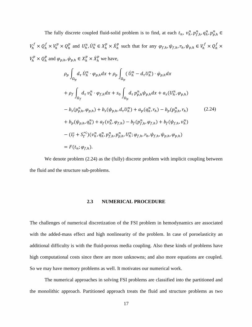
17

The fully discrete coupled fluid-solid problem is to find, at each 𝑡𝑡𝑖𝑖, 𝜕𝜕ℎ𝑖𝑖,𝑝𝑝𝑓𝑓,ℎ𝑖𝑖 , 𝑞𝑞ℎ𝑖𝑖,𝑝𝑝𝑝𝑝,ℎ

𝑖𝑖 ∈

𝑉𝑉ℎ𝑓𝑓 × 𝑄𝑄ℎ


𝑝𝑝 and 𝑈𝑈ℎ𝑖𝑖, �̇�𝑈ℎ𝑖𝑖 ∈ 𝑋𝑋ℎ𝑝𝑝 × �̇�𝑋ℎ

𝑝𝑝 such that for any 𝜑𝜑𝑓𝑓,ℎ,𝜓𝜓𝑓𝑓,ℎ, 𝑟𝑟ℎ,𝜓𝜓𝑝𝑝,ℎ ∈ 𝑉𝑉ℎ𝑓𝑓 × 𝑄𝑄ℎ

𝑓𝑓 ×

𝑉𝑉ℎ𝑝𝑝 × 𝑄𝑄ℎ

𝑝𝑝 and 𝜑𝜑𝑝𝑝,ℎ, �̇�𝜑𝑝𝑝,ℎ ∈ 𝑋𝑋ℎ𝑝𝑝 × �̇�𝑋ℎ

𝑝𝑝 we have,

𝜌𝜌𝑝𝑝 � 𝑎𝑎𝜏𝜏Ω𝑝𝑝

�̇�𝑈ℎ𝑖𝑖 ⋅ 𝜑𝜑𝑝𝑝,ℎ𝑎𝑎𝑑𝑑 + 𝜌𝜌𝑝𝑝 � (Ω𝑝𝑝

�̇�𝑈ℎ𝑖𝑖 − 𝑎𝑎𝜏𝜏𝑈𝑈ℎ𝑖𝑖) ⋅ �̇�𝜑𝑝𝑝,ℎ𝑎𝑎𝑑𝑑

+ 𝜌𝜌𝑓𝑓 � 𝑎𝑎𝜏𝜏Ω𝑓𝑓

𝜕𝜕ℎ𝑖𝑖 ⋅ 𝜑𝜑𝑓𝑓,ℎ𝑎𝑎𝑑𝑑 + 𝑠𝑠0 � 𝑎𝑎𝜏𝜏Ω𝑝𝑝

𝑝𝑝𝑝𝑝,ℎ𝑖𝑖 𝜓𝜓𝑝𝑝,ℎ𝑎𝑎𝑑𝑑 + 𝑎𝑎𝑠𝑠(𝑈𝑈ℎ𝑖𝑖,𝜑𝜑𝑝𝑝,ℎ)

− 𝑏𝑏𝑠𝑠(𝑝𝑝𝑝𝑝,ℎ𝑖𝑖 ,𝜑𝜑𝑝𝑝,ℎ) + 𝑏𝑏𝑠𝑠(𝜓𝜓𝑝𝑝,ℎ,𝑎𝑎𝜏𝜏𝑈𝑈ℎ𝑖𝑖) + 𝑎𝑎𝑝𝑝(𝑞𝑞ℎ𝑖𝑖, 𝑟𝑟ℎ) − 𝑏𝑏𝑝𝑝(𝑝𝑝𝑝𝑝,ℎ

𝑖𝑖 , 𝑟𝑟ℎ)

+ 𝑏𝑏𝑝𝑝(𝜓𝜓𝑝𝑝,ℎ,𝑞𝑞ℎ𝑖𝑖) + 𝑎𝑎𝑓𝑓(𝜕𝜕ℎ𝑖𝑖,𝜑𝜑𝑓𝑓,ℎ) − 𝑏𝑏𝑓𝑓(𝑝𝑝𝑓𝑓,ℎ𝑖𝑖 ,𝜑𝜑𝑓𝑓,ℎ) + 𝑏𝑏𝑓𝑓(𝜓𝜓𝑓𝑓,ℎ, 𝜕𝜕ℎ𝑖𝑖)

− (𝐼𝐼Γ∗ + 𝑆𝑆Γ∗𝜍𝜍)(𝜕𝜕ℎ𝑖𝑖, 𝑞𝑞ℎ𝑖𝑖,𝑝𝑝𝑓𝑓,ℎ

𝑖𝑖 ,𝑝𝑝𝑝𝑝,ℎ𝑖𝑖 ,𝑈𝑈ℎ𝑖𝑖;𝜑𝜑𝑓𝑓,ℎ, 𝑟𝑟ℎ,𝜓𝜓𝑓𝑓,ℎ,𝜓𝜓𝑝𝑝,ℎ,𝜑𝜑𝑝𝑝,ℎ)

= 𝐹𝐹(𝑡𝑡𝑖𝑖;𝜑𝜑𝑓𝑓,ℎ).

(2.24)

We denote problem (2.24) as the (fully) discrete problem with implicit coupling between

the fluid and the structure sub-problems.

2.3 NUMERICAL PROCEDURE

The challenges of numerical discretization of the FSI problem in hemodynamics are associated

with the added-mass effect and high nonlinearity of the problem. In case of poroelasticity an

additional difficulty is with the fluid-porous media coupling. Also these kinds of problems have

high computational costs since there are more unknowns; and also more equations are coupled.

So we may have memory problems as well. It motivates our numerical work.

The numerical approaches in solving FSI problems are classified into the partitioned and

the monolithic approach. Partitioned approach treats the fluid and structure problems as two

18

computational fields, which can be solved using two distinct solvers. The interface conditions

between the fluid and structure are solved through loosely or strongly coupled algorithms.

Monolithic approach treats the fluid and the structure as a single system and the interfacial

conditions are implicit in the solution procedure.

We have addressed both approaches for solving this problem. Indeed, it is expensive to

solve this complex system by using the traditional monolithic methods even though they are

usually stable and accurate. Hence, it is important to develop new methods to solve it in

decoupled ways. Since splitting of the problem degrades the approximation properties, we first

propose a loosely coupled method and then we suggest that the loosely coupled scheme serve as

a preconditioner for the global monolithic solution approach. At the best of our knowledge, it is

the first time that this approach is adopted for fluid porous structure interaction problems.

2.3.1 Partitioned scheme

When enforced by Nitsche’s method, the interface conditions appear in the variational

formulation in a modular form. As a result, using time lagging, it is straightforward to design

various loosely coupled algorithms to solve each equation of the problem independently from the

others. If we finally proceed to solve all the problems independently, we obtain the explicit

algorithm reported below. We also formulate explicitly the governing and interface conditions

that are enforced in practice when each sub-problem is solved. The stability analysis is provide in

[27].

19

Sub-problem 1: given 𝜕𝜕ℎ𝑖𝑖−1,𝑝𝑝𝑓𝑓,ℎ𝑖𝑖−1, 𝑞𝑞ℎ𝑖𝑖−1,𝑝𝑝𝑝𝑝,ℎ

𝑖𝑖−1 find 𝑈𝑈ℎ𝑖𝑖, �̇�𝑈ℎ𝑖𝑖 in Ω𝑝𝑝 such that:

𝜌𝜌𝑝𝑝 � 𝑎𝑎𝜏𝜏Ω𝑝𝑝

�̇�𝑈ℎ𝑖𝑖 ⋅ 𝜑𝜑𝑝𝑝,ℎ + 𝜌𝜌𝑝𝑝 � (Ω𝑝𝑝

�̇�𝑈ℎ𝑖𝑖 − 𝑎𝑎𝜏𝜏𝑈𝑈ℎ𝑖𝑖) ⋅ �̇�𝜑𝑝𝑝,ℎ + 𝑎𝑎𝑠𝑠(𝑈𝑈ℎ𝑖𝑖,𝜑𝜑𝑝𝑝,ℎ) + �𝛾𝛾𝑓𝑓Γ

𝜇𝜇𝑓𝑓ℎ−1𝑎𝑎𝜏𝜏𝑈𝑈ℎ𝑖𝑖 ⋅ 𝑡𝑡𝑝𝑝 𝜑𝜑𝑝𝑝,ℎ

⋅ 𝑡𝑡𝑝𝑝 + �𝛾𝛾𝑓𝑓Γ

𝜇𝜇𝑓𝑓ℎ−1𝑎𝑎𝜏𝜏𝑈𝑈ℎ𝑖𝑖 ⋅ 𝑖𝑖𝑝𝑝 𝜑𝜑𝑝𝑝,ℎ ⋅ 𝑖𝑖𝑝𝑝

= 𝑏𝑏𝑠𝑠(𝑝𝑝𝑝𝑝,ℎ𝑖𝑖−1,𝜑𝜑𝑝𝑝,ℎ) −�𝑖𝑖𝑝𝑝

Γ⋅ 𝜎𝜎𝑓𝑓,ℎ

𝑖𝑖−1𝑖𝑖𝑝𝑝 (−𝜑𝜑𝑝𝑝,ℎ) ⋅ 𝑖𝑖𝑝𝑝 − �𝑡𝑡𝑝𝑝Γ

⋅ 𝜎𝜎𝑓𝑓,ℎ𝑖𝑖−1𝑖𝑖𝑝𝑝(−𝜑𝜑𝑝𝑝,ℎ) ⋅ 𝑡𝑡𝑝𝑝

+ �𝛾𝛾𝑓𝑓Γ

𝜇𝜇𝑓𝑓ℎ−1𝜕𝜕ℎ𝑖𝑖−1 ⋅ 𝑡𝑡𝑝𝑝 𝜑𝜑𝑝𝑝,ℎ ⋅ 𝑡𝑡𝑝𝑝 + �𝛾𝛾𝑓𝑓Γ

𝜇𝜇𝑓𝑓ℎ−1(𝜕𝜕ℎ𝑖𝑖−1 − 𝑞𝑞ℎ𝑖𝑖−1) ⋅ 𝑖𝑖𝑝𝑝 𝜑𝜑𝑝𝑝,ℎ ⋅ 𝑖𝑖𝑝𝑝.

This problem is equivalent to solving the elastodynamics equation, namely (2.5), where

the pressure term has been time-lagged, complemented with the following Robin-type boundary

condition on Γ:

𝑖𝑖𝑝𝑝 ⋅ 𝜎𝜎𝑝𝑝𝑖𝑖𝑖𝑖𝑝𝑝 = 𝑖𝑖𝑝𝑝 ⋅ (𝜎𝜎𝑓𝑓)𝑖𝑖−1𝑖𝑖𝑝𝑝 − 𝛾𝛾𝑓𝑓𝜇𝜇𝑓𝑓ℎ−1(𝑎𝑎𝜏𝜏𝑈𝑈𝑖𝑖 − 𝜕𝜕𝑖𝑖−1 + 𝑞𝑞𝑖𝑖−1) ⋅ 𝑖𝑖𝑝𝑝, on Γ,

𝑡𝑡𝑝𝑝 ⋅ 𝜎𝜎𝑝𝑝𝑖𝑖𝑖𝑖𝑝𝑝 = 𝑡𝑡𝑝𝑝 ⋅ (𝜎𝜎𝑓𝑓)𝑖𝑖−1𝑖𝑖𝑝𝑝 − 𝛾𝛾𝑓𝑓𝜇𝜇𝑓𝑓ℎ−1(𝑎𝑎𝜏𝜏𝑈𝑈𝑖𝑖 − 𝜕𝜕𝑖𝑖−1) ⋅ 𝑡𝑡𝑝𝑝, on Γ.

Also the terms involving stress in the fluid are evaluated at the previous time step, to

improve the stability of the explicit coupling.

Sub-problem 2: given 𝜕𝜕ℎ𝑖𝑖−1,𝑝𝑝𝑓𝑓,ℎ𝑖𝑖−1 and 𝑈𝑈ℎ𝑖𝑖, find 𝑞𝑞ℎ,𝑝𝑝𝑝𝑝,ℎ

𝑖𝑖 in Ω𝑝𝑝 such that:

𝑠𝑠0 � 𝑎𝑎𝜏𝜏Ω𝑝𝑝

𝑝𝑝𝑝𝑝,ℎ𝑖𝑖 𝜓𝜓𝑝𝑝,ℎ𝑎𝑎𝑑𝑑 + 𝑎𝑎𝑝𝑝(𝑞𝑞ℎ𝑖𝑖, 𝑟𝑟ℎ) − 𝑏𝑏𝑝𝑝�𝑝𝑝𝑝𝑝,ℎ

𝑖𝑖 , 𝑟𝑟ℎ� + 𝑏𝑏𝑝𝑝�𝜓𝜓𝑝𝑝,ℎ, 𝑞𝑞ℎ𝑖𝑖�

+ 𝑠𝑠𝑓𝑓,𝑞𝑞�𝑎𝑎𝜏𝜏𝑞𝑞ℎ ⋅ 𝑖𝑖𝑝𝑝, 𝑟𝑟ℎ ⋅ 𝑖𝑖𝑝𝑝� + �𝛾𝛾𝑓𝑓Γ

𝜇𝜇𝑓𝑓ℎ−1𝑞𝑞ℎ𝑖𝑖 ⋅ 𝑖𝑖𝑝𝑝 𝑟𝑟ℎ ⋅ 𝑖𝑖𝑝𝑝

= −𝑏𝑏𝑠𝑠�𝜓𝜓𝑝𝑝,ℎ,𝑎𝑎𝜏𝜏𝑈𝑈ℎ𝑖𝑖� + �𝛾𝛾𝑓𝑓Γ

𝜇𝜇𝑓𝑓ℎ−1(𝜕𝜕ℎ𝑖𝑖−1 − 𝑎𝑎𝜏𝜏𝑈𝑈ℎ𝑖𝑖−1) ⋅ 𝑖𝑖𝑝𝑝 𝑟𝑟ℎ ⋅ 𝑖𝑖𝑝𝑝

+ �𝑖𝑖𝑝𝑝Γ

⋅ 𝜎𝜎𝑓𝑓,ℎ𝑖𝑖−1𝑖𝑖𝑝𝑝 𝑟𝑟ℎ ⋅ 𝑖𝑖𝑝𝑝.

20

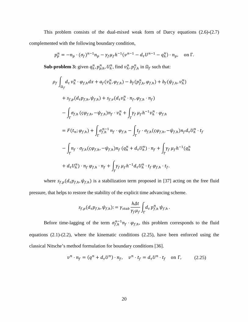
This problem consists of the dual-mixed weak form of Darcy equations (2.6)-(2.7)

complemented with the following boundary condition,

𝑝𝑝𝑝𝑝𝑖𝑖 = −𝑖𝑖𝑝𝑝 ⋅ (𝜎𝜎𝑓𝑓)𝑖𝑖−1𝑖𝑖𝑝𝑝 − 𝛾𝛾𝑓𝑓𝜇𝜇𝑓𝑓ℎ−1(𝜕𝜕𝑖𝑖−1 − 𝑎𝑎𝜏𝜏𝑈𝑈𝑖𝑖−1 − 𝑞𝑞ℎ𝑖𝑖) ⋅ 𝑖𝑖𝑝𝑝, on Γ.

Sub-problem 3: given 𝑞𝑞ℎ𝑖𝑖,𝑝𝑝𝑝𝑝,ℎ𝑖𝑖 ,𝑈𝑈ℎ𝑖𝑖, find 𝜕𝜕ℎ𝑖𝑖, 𝑝𝑝𝑓𝑓,ℎ

𝑖𝑖 in Ω𝑓𝑓 such that:

𝜌𝜌𝑓𝑓 � 𝑎𝑎𝜏𝜏Ω𝑓𝑓

𝜕𝜕ℎ𝑖𝑖 ⋅ 𝜑𝜑𝑓𝑓,ℎ𝑎𝑎𝑑𝑑 + 𝑎𝑎𝑓𝑓(𝜕𝜕ℎ𝑖𝑖,𝜑𝜑𝑓𝑓,ℎ) − 𝑏𝑏𝑓𝑓(𝑝𝑝𝑓𝑓,ℎ𝑖𝑖 ,𝜑𝜑𝑓𝑓,ℎ) + 𝑏𝑏𝑓𝑓(𝜓𝜓𝑓𝑓,ℎ, 𝜕𝜕ℎ𝑖𝑖)

+ 𝑠𝑠𝑓𝑓,𝑝𝑝(𝑎𝑎𝜏𝜏𝑝𝑝𝑓𝑓,ℎ,𝜓𝜓𝑓𝑓,ℎ) + 𝑠𝑠𝑓𝑓,𝑣𝑣(𝑎𝑎𝜏𝜏𝜕𝜕ℎ𝑖𝑖 ⋅ 𝑖𝑖𝑓𝑓 ,𝜑𝜑𝑓𝑓,ℎ ⋅ 𝑖𝑖𝑓𝑓)

−�𝜎𝜎𝑓𝑓,ℎΓ

(𝜍𝜍𝜑𝜑𝑓𝑓,ℎ,−𝜓𝜓𝑓𝑓,ℎ)𝑖𝑖𝑓𝑓 ⋅ 𝜕𝜕ℎ𝑖𝑖 + �𝛾𝛾𝑓𝑓Γ

𝜇𝜇𝑓𝑓ℎ−1𝜕𝜕ℎ𝑖𝑖 ⋅ 𝜑𝜑𝑓𝑓,ℎ

= 𝐹𝐹(𝑡𝑡𝑖𝑖;𝜑𝜑𝑓𝑓,ℎ) + �𝜎𝜎𝑓𝑓,ℎ𝑖𝑖−1

Γ𝑖𝑖𝑓𝑓 ⋅ 𝜑𝜑𝑓𝑓,ℎ − �𝑡𝑡𝑓𝑓

Γ⋅ 𝜎𝜎𝑓𝑓,ℎ(𝜍𝜍𝜑𝜑𝑓𝑓,ℎ,−𝜓𝜓𝑓𝑓,ℎ)𝑖𝑖𝑓𝑓𝑎𝑎𝜏𝜏𝑈𝑈ℎ𝑖𝑖 ⋅ 𝑡𝑡𝑓𝑓

− �𝑖𝑖𝑓𝑓Γ

⋅ 𝜎𝜎𝑓𝑓,ℎ(𝜍𝜍𝜑𝜑𝑓𝑓,ℎ,−𝜓𝜓𝑓𝑓,ℎ)𝑖𝑖𝑓𝑓 (𝑞𝑞ℎ𝑖𝑖 + 𝑎𝑎𝜏𝜏𝑈𝑈ℎ𝑖𝑖) ⋅ 𝑖𝑖𝑓𝑓 + �𝛾𝛾𝑓𝑓Γ

𝜇𝜇𝑓𝑓ℎ−1(𝑞𝑞ℎ𝑖𝑖

+ 𝑎𝑎𝜏𝜏𝑈𝑈ℎ𝑖𝑖) ⋅ 𝑖𝑖𝑓𝑓 𝜑𝜑𝑓𝑓,ℎ ⋅ 𝑖𝑖𝑓𝑓 + �𝛾𝛾𝑓𝑓Γ

𝜇𝜇𝑓𝑓ℎ−1𝑎𝑎𝜏𝜏𝑈𝑈ℎ𝑖𝑖 ⋅ 𝑡𝑡𝑓𝑓 𝜑𝜑𝑓𝑓,ℎ ⋅ 𝑡𝑡𝑓𝑓 .

where 𝑠𝑠𝑓𝑓,𝑝𝑝(𝑎𝑎𝜏𝜏𝑝𝑝𝑓𝑓,ℎ,𝜓𝜓𝑓𝑓,ℎ) is a stabilization term proposed in [37] acting on the free fluid

pressure, that helps to restore the stability of the explicit time advancing scheme.

𝑠𝑠𝑓𝑓,𝑝𝑝(𝑎𝑎𝜏𝜏𝑝𝑝𝑓𝑓,ℎ,𝜓𝜓𝑓𝑓,ℎ): = 𝛾𝛾𝑠𝑠𝑜𝑜𝑠𝑠𝑠𝑠ℎ𝛥𝛥𝑡𝑡𝛾𝛾𝑓𝑓𝜇𝜇𝑓𝑓

�𝑎𝑎𝜏𝜏Γ

𝑝𝑝𝑓𝑓,ℎ𝑖𝑖 𝜓𝜓𝑓𝑓,ℎ .

Before time-lagging of the term 𝜎𝜎𝑓𝑓,ℎ𝑖𝑖−1𝑖𝑖𝑓𝑓 ⋅ 𝜑𝜑𝑓𝑓,ℎ, this problem corresponds to the fluid

equations (2.1)-(2.2), where the kinematic conditions (2.25), have been enforced using the

classical Nitsche’s method formulation for boundary conditions [36].

𝜕𝜕𝑖𝑖 ⋅ 𝑖𝑖𝑓𝑓 = (𝑞𝑞𝑖𝑖 + 𝑎𝑎𝜏𝜏𝑈𝑈𝑖𝑖) ⋅ 𝑖𝑖𝑓𝑓 , 𝜕𝜕𝑖𝑖 ⋅ 𝑡𝑡𝑓𝑓 = 𝑎𝑎𝜏𝜏𝑈𝑈𝑖𝑖 ⋅ 𝑡𝑡𝑓𝑓 on Γ, (2.25)

21

We observe that new stabilization terms 𝑠𝑠𝑓𝑓,𝑣𝑣, 𝑠𝑠𝑓𝑓,𝑞𝑞 have been introduced into the problem

formulation. Their role is to control the increment of 𝜕𝜕ℎ𝑖𝑖, 𝑞𝑞ℎ𝑖𝑖 over two subsequent time steps,

namely:

𝑠𝑠𝑓𝑓,𝑞𝑞(𝑎𝑎𝜏𝜏𝑞𝑞ℎ𝑖𝑖 ⋅ 𝑖𝑖, 𝑟𝑟ℎ ⋅ 𝑖𝑖) = 𝛾𝛾𝑠𝑠𝑜𝑜𝑠𝑠𝑠𝑠′ 𝛾𝛾𝑓𝑓𝜇𝜇𝑓𝑓𝛥𝛥𝑡𝑡ℎ�𝑎𝑎𝜏𝜏Γ

𝑞𝑞ℎ𝑖𝑖 ⋅ 𝑖𝑖𝑟𝑟ℎ ⋅ 𝑖𝑖 ,

𝑠𝑠𝑓𝑓,𝑣𝑣(𝑎𝑎𝜏𝜏𝜕𝜕ℎ𝑖𝑖 ⋅ 𝑖𝑖,𝜑𝜑𝑓𝑓,ℎ ⋅ 𝑖𝑖) = 𝛾𝛾𝑠𝑠𝑜𝑜𝑠𝑠𝑠𝑠′ 𝛾𝛾𝑓𝑓𝜇𝜇𝑓𝑓𝛥𝛥𝑡𝑡ℎ�𝑎𝑎𝜏𝜏Γ

𝜕𝜕ℎ𝑖𝑖 ⋅ 𝑖𝑖𝜑𝜑𝑓𝑓,ℎ ⋅ 𝑖𝑖 .

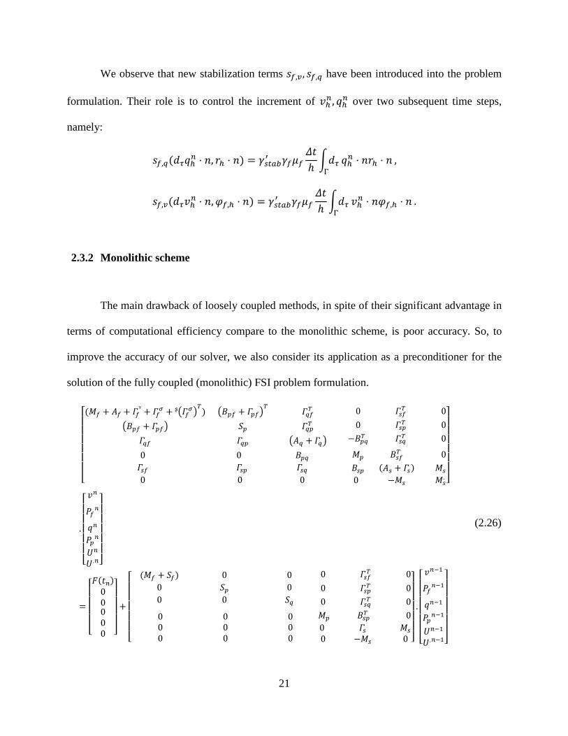
2.3.2 Monolithic scheme

The main drawback of loosely coupled methods, in spite of their significant advantage in

terms of computational efficiency compare to the monolithic scheme, is poor accuracy. So, to

improve the accuracy of our solver, we also consider its application as a preconditioner for the

solution of the fully coupled (monolithic) FSI problem formulation.

⎣⎢⎢⎢⎢⎢⎢⎡(𝑀𝑀𝑓𝑓 + 𝐴𝐴𝑓𝑓 + 𝛤𝛤𝑓𝑓ᵞ + 𝛤𝛤𝑓𝑓𝜎𝜎 + ᶳ�𝛤𝛤𝑓𝑓𝜎𝜎�

𝑇𝑇) �𝐵𝐵𝑝𝑝𝑓𝑓 + 𝛤𝛤𝑝𝑝𝑓𝑓�𝑇𝑇 𝛤𝛤𝑞𝑞𝑓𝑓𝑇𝑇

�𝐵𝐵𝑝𝑝𝑓𝑓 + 𝛤𝛤𝑝𝑝𝑓𝑓� 𝑆𝑆𝑝𝑝 𝛤𝛤𝑞𝑞𝑝𝑝𝑇𝑇

𝛤𝛤𝑞𝑞𝑓𝑓 𝛤𝛤𝑞𝑞𝑝𝑝 �𝐴𝐴𝑞𝑞 + 𝛤𝛤𝑞𝑞�

0 𝛤𝛤𝑠𝑠𝑓𝑓𝑇𝑇 00 𝛤𝛤𝑠𝑠𝑝𝑝𝑇𝑇 0

−𝐵𝐵𝑝𝑝𝑞𝑞𝑇𝑇 𝛤𝛤𝑠𝑠𝑞𝑞𝑇𝑇 0

0 0 𝐵𝐵𝑝𝑝𝑞𝑞 𝛤𝛤𝑠𝑠𝑓𝑓 𝛤𝛤𝑠𝑠𝑝𝑝 𝛤𝛤𝑠𝑠𝑞𝑞 0 0 0

𝑀𝑀𝑝𝑝 𝐵𝐵𝑠𝑠𝑓𝑓𝑇𝑇 0 𝐵𝐵𝑠𝑠𝑝𝑝 (𝐴𝐴𝑠𝑠 + 𝛤𝛤𝑠𝑠) 𝑀𝑀𝑠𝑠

0 −𝑀𝑀𝑠𝑠 𝑀𝑀𝑠𝑠. ⎦⎥⎥⎥⎥⎥⎥⎤

.

⎣⎢⎢⎢⎢⎢⎡𝜕𝜕𝑖𝑖

𝑃𝑃𝑓𝑓𝑖𝑖

𝑞𝑞𝑖𝑖

𝑃𝑃𝑝𝑝𝑖𝑖

𝑈𝑈𝑖𝑖

𝑈𝑈.𝑖𝑖⎦⎥⎥⎥⎥⎥⎤

=

⎣⎢⎢⎢⎢⎡𝐹𝐹

(𝑡𝑡𝑖𝑖)00000 ⎦

⎥⎥⎥⎥⎤

+

⎣⎢⎢⎢⎢⎢⎡ (𝑀𝑀𝑓𝑓 + 𝑆𝑆𝑓𝑓) 0 0

0 𝑆𝑆𝑝𝑝 00 0 𝑆𝑆𝑞𝑞

0 𝛤𝛤𝑠𝑠𝑓𝑓𝑇𝑇 00 𝛤𝛤𝑠𝑠𝑝𝑝𝑇𝑇 00 𝛤𝛤𝑠𝑠𝑞𝑞𝑇𝑇 0

0 0 00 0 00 0 0

𝑀𝑀𝑝𝑝 𝐵𝐵𝑠𝑠𝑝𝑝𝑇𝑇 0 0 𝛤𝛤𝑠𝑠 𝑀𝑀𝑠𝑠 0 −𝑀𝑀𝑠𝑠 0 ⎦

⎥⎥⎥⎥⎥⎤

.

⎣⎢⎢⎢⎢⎢⎢⎡ 𝜕𝜕

𝑖𝑖−1

𝑃𝑃𝑓𝑓𝑖𝑖−1

𝑞𝑞𝑖𝑖−1

𝑃𝑃𝑝𝑝𝑖𝑖−1

𝑈𝑈𝑖𝑖−1

𝑈𝑈.𝑖𝑖−1⎦⎥⎥⎥⎥⎥⎥⎤

(2.26)

22

In this way, we blend the computational efficiency of the loosely couples scheme with

the accuracy of the monolithic ones. The block structure of the algebraic monolithic problem is

illustrated (2.26).

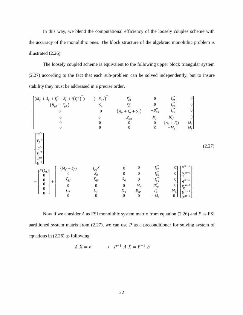
The loosely coupled scheme is equivalent to the following upper block triangular system

(2.27) according to the fact that each sub-problem can be solved independently, but to insure

stability they must be addressed in a precise order,

⎣⎢⎢⎢⎢⎢⎢⎡(𝑀𝑀𝑓𝑓 + 𝐴𝐴𝑓𝑓 + 𝛤𝛤𝑓𝑓ᵞ + 𝑆𝑆𝑓𝑓 + ᶳ�𝛤𝛤𝑓𝑓𝜎𝜎�

𝑇𝑇) �−𝐵𝐵𝑝𝑝𝑓𝑓�𝑇𝑇 𝛤𝛤𝑞𝑞𝑓𝑓𝑇𝑇


0 0 �𝐴𝐴𝑞𝑞 + 𝛤𝛤𝑞𝑞 + 𝑆𝑆𝑞𝑞�



0 0 𝐵𝐵𝑝𝑝𝑞𝑞 0 0 0 0 0 0

𝑀𝑀𝑝𝑝 𝐵𝐵𝑠𝑠𝑓𝑓𝑇𝑇 0 0 (𝐴𝐴𝑠𝑠 + 𝛤𝛤𝑠𝑠) 𝑀𝑀𝑠𝑠 0 −𝑀𝑀𝑠𝑠 𝑀𝑀𝑠𝑠

. ⎦⎥⎥⎥⎥⎥⎥⎤

.

⎣⎢⎢⎢⎢⎢⎡𝜕𝜕𝑖𝑖

𝑃𝑃𝑓𝑓𝑖𝑖

𝑞𝑞𝑖𝑖

𝑃𝑃𝑝𝑝𝑖𝑖

𝑈𝑈𝑖𝑖

𝑈𝑈 .𝑖𝑖⎦⎥⎥⎥⎥⎥⎤

=

⎣⎢⎢⎢⎢⎡𝐹𝐹(𝑡𝑡𝑖𝑖)

00000 ⎦

⎥⎥⎥⎥⎤

+

⎣⎢⎢⎢⎢⎢⎡ (𝑀𝑀𝑓𝑓 + 𝑆𝑆𝑓𝑓) 𝛤𝛤𝑝𝑝𝑓𝑓𝑇𝑇 0

0 𝑆𝑆𝑝𝑝 0𝛤𝛤𝑞𝑞𝑓𝑓 𝛤𝛤𝑞𝑞𝑝𝑝 𝑆𝑆𝑞𝑞

0 𝛤𝛤𝑠𝑠𝑓𝑓𝑇𝑇 00 𝛤𝛤𝑠𝑠𝑝𝑝𝑇𝑇 00 𝛤𝛤𝑠𝑠𝑞𝑞𝑇𝑇 0

0 0 0𝛤𝛤𝑠𝑠𝑓𝑓 𝛤𝛤𝑠𝑠𝑝𝑝 𝛤𝛤𝑠𝑠𝑞𝑞0 0 0

𝑀𝑀𝑝𝑝 𝐵𝐵𝑠𝑠𝑝𝑝𝑇𝑇 0 𝐵𝐵𝑠𝑠𝑝𝑝 𝛤𝛤𝑠𝑠 𝑀𝑀𝑠𝑠 0 −𝑀𝑀𝑠𝑠 0 ⎦

⎥⎥⎥⎥⎥⎤

.

⎣⎢⎢⎢⎢⎢⎢⎡ 𝜕𝜕

𝑖𝑖−1

𝑃𝑃𝑓𝑓𝑖𝑖−1

𝑞𝑞𝑖𝑖−1

𝑃𝑃𝑝𝑝𝑖𝑖−1

𝑈𝑈𝑖𝑖−1

𝑈𝑈.𝑖𝑖−1⎦⎥⎥⎥⎥⎥⎥⎤

(2.27)

Now if we consider A as FSI monolithic system matrix from equation (2.26) and P as FSI

partitioned system matrix from (2.27), we can use P as a preconditioner for solving system of

equations in (2.26) as following:

𝐴𝐴.𝑋𝑋 = 𝑏𝑏 → 𝑃𝑃−1.𝐴𝐴.𝑋𝑋 = 𝑃𝑃−1. 𝑏𝑏

23

Where:

𝑃𝑃

=

⎣⎢⎢⎢⎢⎢⎢⎡(𝑀𝑀𝑓𝑓 + 𝐴𝐴𝑓𝑓 + 𝛤𝛤𝑓𝑓ᵞ + 𝑆𝑆𝑓𝑓 + ᶳ�𝛤𝛤𝑓𝑓𝜎𝜎�

𝑇𝑇) �−𝐵𝐵𝑝𝑝𝑓𝑓�𝑇𝑇 𝛤𝛤𝑞𝑞𝑓𝑓𝑇𝑇


0 0 �𝐴𝐴𝑞𝑞 + 𝛤𝛤𝑞𝑞 + 𝑆𝑆𝑞𝑞�



0 0 𝐵𝐵𝑝𝑝𝑞𝑞 0 0 0 0 0 0

𝑀𝑀𝑝𝑝 𝐵𝐵𝑠𝑠𝑓𝑓𝑇𝑇 0 0 (𝐴𝐴𝑠𝑠 + 𝛤𝛤𝑠𝑠) 𝑀𝑀𝑠𝑠 0 −𝑀𝑀𝑠𝑠 𝑀𝑀𝑠𝑠

. ⎦⎥⎥⎥⎥⎥⎥⎤

(2.28)

𝐴𝐴

=

⎣⎢⎢⎢⎢⎢⎢⎡(𝑀𝑀𝑓𝑓 + 𝐴𝐴𝑓𝑓 + 𝛤𝛤𝑓𝑓ᵞ + 𝛤𝛤𝑓𝑓𝜎𝜎 + ᶳ�𝛤𝛤𝑓𝑓𝜎𝜎�

𝑇𝑇) �𝐵𝐵𝑝𝑝𝑓𝑓 + 𝛤𝛤𝑝𝑝𝑓𝑓�𝑇𝑇 𝛤𝛤𝑞𝑞𝑓𝑓𝑇𝑇


𝛤𝛤𝑞𝑞𝑓𝑓 𝛤𝛤𝑞𝑞𝑝𝑝 �𝐴𝐴𝑞𝑞 + 𝛤𝛤𝑞𝑞�



0 0 𝐵𝐵𝑝𝑝𝑞𝑞 𝛤𝛤𝑠𝑠𝑓𝑓 𝛤𝛤𝑠𝑠𝑝𝑝 𝛤𝛤𝑠𝑠𝑞𝑞 0 0 0

𝑀𝑀𝑝𝑝 𝐵𝐵𝑠𝑠𝑓𝑓𝑇𝑇 0 𝐵𝐵𝑠𝑠𝑝𝑝 (𝐴𝐴𝑠𝑠 + 𝛤𝛤𝑠𝑠) 𝑀𝑀𝑠𝑠

0 −𝑀𝑀𝑠𝑠 𝑀𝑀𝑠𝑠. ⎦⎥⎥⎥⎥⎥⎥⎤

(2.29)

The preconditioner divides the problem into 3 sub-problems that can be solved with

backward substitution:

�𝐹𝐹𝐹𝐹 𝐹𝐹𝑀𝑀 𝐹𝐹𝑆𝑆0 𝑀𝑀𝑀𝑀 𝑀𝑀𝑆𝑆0 0 𝑆𝑆𝑆𝑆

� . �𝑑𝑑𝑓𝑓𝑑𝑑𝑚𝑚𝑑𝑑𝑠𝑠� = �

𝑏𝑏𝑓𝑓𝑏𝑏𝑚𝑚𝑏𝑏𝑠𝑠� (2.30)

Step 1 𝑏𝑏𝑠𝑠 = 𝑆𝑆𝑆𝑆/𝑑𝑑𝑠𝑠

Step 2 𝑏𝑏𝑚𝑚 = 𝑀𝑀𝑀𝑀 ∗ 𝑑𝑑𝑚𝑚 + 𝑀𝑀𝑆𝑆 ∗ 𝑑𝑑𝑠𝑠 → 𝑑𝑑𝑚𝑚 = (𝑏𝑏𝑚𝑚 − 𝑀𝑀𝑆𝑆 ∗ 𝑑𝑑𝑠𝑠)/𝑀𝑀𝑀𝑀

Step 3 𝑏𝑏𝑓𝑓 = 𝐹𝐹𝐹𝐹 ∗ 𝑑𝑑𝑓𝑓 + 𝐹𝐹𝑀𝑀 ∗ 𝑑𝑑𝑚𝑚 + 𝐹𝐹𝑆𝑆 ∗ 𝑑𝑑𝑠𝑠 → 𝑑𝑑𝑓𝑓 = (𝑏𝑏𝑓𝑓 − 𝐹𝐹𝑀𝑀 ∗ 𝑑𝑑𝑚𝑚 + 𝐹𝐹𝑆𝑆 ∗ 𝑑𝑑𝑠𝑠)/𝐹𝐹𝐹𝐹

24

2.4 NUMERICAL SIMULATIONS

In this section we present some numerical results with the aim of testing the methodologies

proposed in previous section. All simulations are obtained using a fixed mesh algorithm and

movement of the fluid domain is not taken into account; but we have performed some additional

simulations using a deformable fluid computational domain and the physiological parameters of

Table 1. The results (published in [40]), confirm that for the considered test case the deformation

of the computational mesh do not play a significant role on the calculated blood flow rate and the

arterial wall displacement.

The approximation space for the fluid flow is based on P2-P1 approximations for velocity

and pressure respectively that ensures inf-sup stability of the scheme and the same finite element

spaces are used for intramural filtration velocity and pressure in the poroelastic wall. We also use

P2 finite elements for the discretization of the structure displacement. Time discretization is

performed using backward Euler scheme and the time step is 1.e-4 second. Also, we have used

the following values: 𝛾𝛾𝑓𝑓 = 2500, 𝛾𝛾𝑠𝑠𝑜𝑜𝑠𝑠𝑠𝑠 = 1, 𝛾𝛾𝑠𝑠𝑜𝑜𝑠𝑠𝑠𝑠′ = 0.

All the numerical computations have been performed using the Finite Element code

Freefem++ [41]. For Fluid-Structure Interaction problem in poroelastic media, the solution of

equations for general parameters and problem configuration needs advanced computational tools

and can hardly be handled by commercial packages. So, we tested different language

environment (FEniCS, FreeFem++) and finally we chose FreeFem++ because it has less

complication in writing variational formulations and also it is flexible for enforcing interface

conditions thanks to automatic interpolation from a mesh to another one. We use this

interpolation is for transferring data between fluid and structure grids.

25

2.4.1 FSI analysis of pulsatile flow in a compliant channel

We consider a classical benchmark problem used for FSI problems problem that has been used in

several works [37, 42]. We adopt a geometrical model that consists of a 2D poroelastic structure

superposed to a 2D fluid channel. The model represents a straight vessel of radius 0.5 cm, length

6 cm, and the surrounding structure has a thickness of 0.1 cm. This numerical experiment

consists in studying the propagation of a single pressure wave with amplitude comparable to the

pressure difference between systolic and diastolic phases of a heartbeat.

𝑃𝑃𝑖𝑖𝑖𝑖(𝑡𝑡) = �𝑝𝑝𝑚𝑚𝑠𝑠𝑒𝑒

2�1 − cos �

2𝜋𝜋𝑡𝑡𝑇𝑇𝑚𝑚𝑠𝑠𝑒𝑒

�� 𝑖𝑖𝑓𝑓 𝑡𝑡 ≤ 𝑇𝑇𝑚𝑚𝑠𝑠𝑒𝑒

0 𝑖𝑖𝑓𝑓 𝑡𝑡 > 𝑇𝑇𝑚𝑚𝑠𝑠𝑒𝑒, (2.31)

Table 1. Fluid and structure parameters

Symbol Unit Values

𝜌𝜌𝑝𝑝 g/cm3 1.1

𝜆𝜆𝑝𝑝 dyne/cm2 4.28×106

𝜇𝜇𝑝𝑝 dyne/cm2 1.07×106

𝛼𝛼 mmHg 1

𝜇𝜇𝑓𝑓 poise 0.035

𝜌𝜌𝑓𝑓 g/cm3 1.1

s0 cm2/dyne 5×10-6

κ cm3 s/g 5×10-9

𝜉𝜉 dyne / cm4 5×107

26

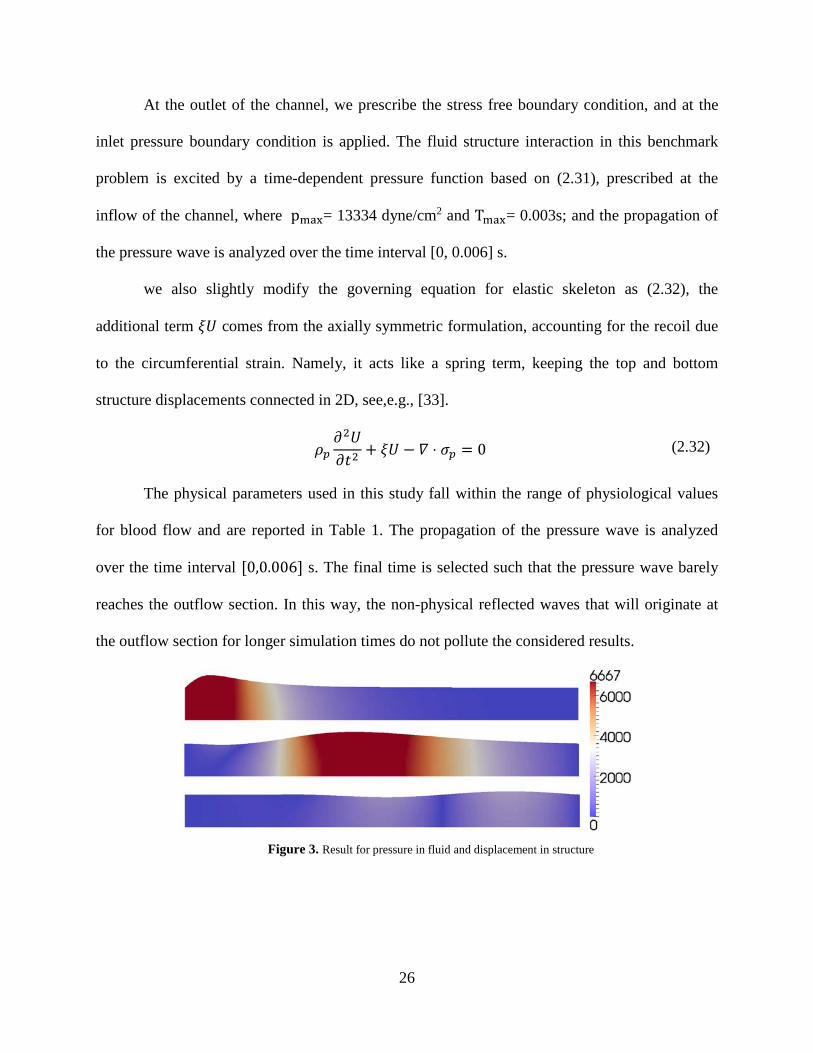
At the outlet of the channel, we prescribe the stress free boundary condition, and at the

inlet pressure boundary condition is applied. The fluid structure interaction in this benchmark

problem is excited by a time-dependent pressure function based on (2.31), prescribed at the

inflow of the channel, where pmax= 13334 dyne/cm2 and Tmax= 0.003s; and the propagation of

the pressure wave is analyzed over the time interval [0, 0.006] s.

we also slightly modify the governing equation for elastic skeleton as (2.32), the

additional term 𝜉𝜉𝑈𝑈 comes from the axially symmetric formulation, accounting for the recoil due

to the circumferential strain. Namely, it acts like a spring term, keeping the top and bottom

structure displacements connected in 2D, see,e.g., [33].


+ 𝜉𝜉𝑈𝑈 − 𝛻𝛻 ⋅ 𝜎𝜎𝑝𝑝 = 0 (2.32)

The physical parameters used in this study fall within the range of physiological values

for blood flow and are reported in Table 1. The propagation of the pressure wave is analyzed

over the time interval [0,0.006] s. The final time is selected such that the pressure wave barely

reaches the outflow section. In this way, the non-physical reflected waves that will originate at

the outflow section for longer simulation times do not pollute the considered results.

Figure 3. Result for pressure in fluid and displacement in structure

27

Some visualizations of the solution, calculated using the settings addressed below, are

reported in Figure 3, and Figure 4. The former, qualitatively shows the propagation of a pressure

wave along the channel, together with the corresponding deformation of the fluid domain at

times 𝑡𝑡1 = 1.5, 𝑡𝑡2 = 3.5, 𝑡𝑡3 = 5.5 ms. For visualization purposes, the vertical displacement is

magnified 100 times in Figure 3. In Figure 4, top panel, we show the vertical displacement of the

interface along the longitudinal axis of the channel. These plots show that the variable inflow

pressure combined with the fluid-structure interaction mechanisms, generates a wave in the

structure that propagates from left to right.

Figure 4. Top panel: displacement of the fluid-structure interface at times 1.5, 3.5 and 5.5 ms from left to right.

Bottom panel: intramural flow q.n at different planes in the arterial wall, located at the interface, at the

intermediate section and at the outer layer

28

On the bottom panel, we show intramural flow 𝑞𝑞ℎ ⋅ 𝑖𝑖 at different planes cutting the

arterial wall in the longitudinal direction. These planes are located at the interface, at the

intermediate section and at the outer layer. These plots show that the peaks of the intramural

flow coincide with the ones of structure displacement and the corresponding peak of arterial

pressure. Furthermore, we notice that the intramural velocity, 𝑞𝑞ℎ ⋅ 𝑖𝑖, decreases as far as the fluid

penetrates further into the wall. This is a consequence of (2.7), which prescribes that 𝛻𝛻 ⋅ 𝑞𝑞ℎ is not

locally preserved, but depends on the rate of change in pressure and volumetric deformation of

the structure. Indeed, this is how the poroelastic coupling shows up in the results.

Moreover, the extension to the 3d model is performed in two different geometries: (1) A

straight vessel of radius 0.5 cm and length 5 cm, the surrounding structure has a thickness of 0.1

cm; (2) A curved vessel of radius 1.5 cm, the surrounding structure has a thickness of 0.3 cm.

The fluid structure interaction in this benchmark problem is excited by pressure profile (2.31),

prescribed at the inflow of the channel and the propagation of the pressure wave is analyzed over

the time interval [0, 0.02] s.

Figure 5. Snapshots of the pressure and solid deformation at 2ms, 4ms, and 6ms from left to right for

straight cylinder

29

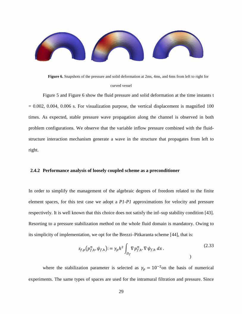
Figure 6. Snapshots of the pressure and solid deformation at 2ms, 4ms, and 6ms from left to right for

curved vessel

Figure 5 and Figure 6 show the fluid pressure and solid deformation at the time instants t

= 0.002, 0.004, 0.006 s. For visualization purpose, the vertical displacement is magnified 100

times. As expected, stable pressure wave propagation along the channel is observed in both

problem configurations. We observe that the variable inflow pressure combined with the fluid-

structure interaction mechanism generate a wave in the structure that propagates from left to

right.

2.4.2 Performance analysis of loosely coupled scheme as a preconditioner

In order to simplify the management of the algebraic degrees of freedom related to the finite

element spaces, for this test case we adopt a P1-P1 approximations for velocity and pressure

respectively. It is well known that this choice does not satisfy the inf–sup stability condition [43].

Resorting to a pressure stabilization method on the whole fluid domain is mandatory. Owing to

its simplicity of implementation, we opt for the Brezzi–Pitkaranta scheme [44], that is:

𝑠𝑠𝑓𝑓,𝑝𝑝�𝑝𝑝𝑓𝑓,ℎ𝑖𝑖 ,𝜓𝜓𝑓𝑓,ℎ�: = 𝛾𝛾𝑝𝑝ℎ2 � ∇

𝛺𝛺𝑓𝑓𝑝𝑝𝑓𝑓,ℎ𝑖𝑖 .∇ 𝜓𝜓𝑓𝑓,ℎ 𝑎𝑎𝑑𝑑 . (2.33

)

where the stabilization parameter is selected as 𝛾𝛾𝑝𝑝 = 10−2on the basis of numerical

experiments. The same types of spaces are used for the intramural filtration and pressure. Since

30

(2.7) is not enforcing the divergence-free constraint exactly, but the material turns out to be

slightly compressible, equal order approximation is stable. We also use P1 finite elements to

approximate the structure velocity and displacement.

The performance of matrix (2.28) used as a preconditioner of (2.29) is quantified by the

numerical experiments reported in Table 2. As an indicator of the system conditioning, we look

at the number of GMRES iterations required to reduce below a given tolerance the relative

residual. The values are calculated on the basis of the first 10 time steps of the simulation.

In the special case of positive definite matrices, the number of iterations (# GMRES)

required to reduce the relative residual of a factor 10𝑃𝑃, can be estimated as # GMRES ≃

𝑝𝑝�𝐾𝐾 ( 𝑃𝑃−1 𝐴𝐴), where K (·) is the spectral condition number. Since the initial relative residual is

one, by definition, (# GMRES) is equivalent to the number of iterations performed until the

relative residual is less than 10−𝑃𝑃. In the experiments that follow, we have used p = 6. As a

result, knowing that the conditioning of the FEM stiffness matrices scales as the square of the

number of degrees of freedom, we expect that # GMRES linearly scales with the number of

degrees of freedom in absence of preconditioners. Optimal preconditioners are those where the

number of GMRES iterations becomes independent of the dimension of the discrete problem.

The results of Table 2 nicely agree with the general GMRES convergence theory, and

confirm that (2.28) behaves as an optimal preconditioner for (2.29). Not only the number of

iterations to solve the preconditioned system is nearly insensitive with respect to the mesh

characteristic size, and consequently the number of degrees of freedom of the discrete problem,

but the number of iterations is significantly smaller than in the non-preconditioned case.

Reminding that the inversion of (2.28) is a relatively inexpensive operation, the preconditioned

algorithm turns out to be a very effective solution method. Table 2 also suggests that the

31

conditioning of the monolithic problem slightly increases when the time step is refined,

especially for coarse meshes, while the good preconditioner performance seems to be unaffected.

It indeed slightly improves, according to the fact that the loosely coupled scheme, and

the related preconditioner, becomes more accurate and effective when the time

discretization step decreases. We have tested this algorithm also using quadratic finite elements,

P2, for all velocities and displacement fields. In the case of the coarsest mesh h = 0.05 cm,

GMRES converges in 613.5 (average) iterations, while solving the preconditioned only requires

11 iterations. The preconditioner seems to scale well also with respect to the FEM polynomial

degree. The good results on preconditioner performance also correspond to a decrease in the

computational time. For h = 0.05, Δt = 10−4, the calculation of 60 time steps of the monolithic

scheme require 4.73 s, while for the preconditioned method the time is 1.85 s. For Δt = 10−5 and

600 time steps the computational times are respectively, 65.8 and 14.6 s.

Table 2. Average number of GMRES iterations for different time steps

Δt=10-4 h=0.05 h=0.025 h=0.0125

#GMRES (monolithic) 211.4 446.4 1282.9

#GMRES (preconditioner) 10.9 12 13.9

Δt=10-5 h=0.05 h=0.025 h=0.0125

#GMRES (monolithic) 362.1 498.3 1194.4

#GMRES (preconditioner) 8 10 12.9

32

2.4.3 Convergence analysis

In this section, we perform the convergence analysis to support the theoretical results on

the accuracy of the numerical scheme provided in section 2.3 . Theoretical results for accuracy of

the proposed scheme are given in Theorem 3 in our paper [27] which shows that the main

drawback of the scheme is related to the splitting of the equations within each time step that

decrease the accuracy. For this purpose, we start our investigation for variation of the time step

Δt.

Since the analytical one is not available in this case, we use the numerical solution

calculated using the monolithic scheme with a small time step equal to Δt = 10−6 s, as reference

solution. This way, we make sure that the splitting error is not polluting the solution, and the

approximation error related to the time discretization scheme is negligible. This solution will be

denoted with the subscript 𝑟𝑟𝑟𝑟𝑓𝑓. To guarantee a sufficient spatial resolution as well as inf-sup

stability, we use P2-P1 approximations for velocity and pressure in the blood flow, combined

with P2-P1 approximation of Darcy’s equation and P2 approximation of the structure

displacement and velocity. We investigate the convergence properties of the scheme in the norm

||| ⋅ |||♥, 𝑁𝑁2 that is used in Theorem 3 in [27]. More precisely, we split it in four parts:

ℰ𝑓𝑓,ℎ𝑁𝑁 ≔ 𝜌𝜌𝑓𝑓 ∥ 𝜕𝜕ℎ𝑁𝑁 − 𝜕𝜕ℎ

𝑁𝑁,𝑟𝑟𝑒𝑒𝑓𝑓 ∥𝐿𝐿2�Ω𝑓𝑓�2 ,

ℰ𝑝𝑝,ℎ𝑁𝑁 (𝑎𝑎) ≔ 𝜌𝜌𝑝𝑝 ∥ �̇�𝑈ℎ𝑁𝑁 − �̇�𝑈ℎ

𝑁𝑁,𝑟𝑟𝑒𝑒𝑓𝑓 ∥𝐿𝐿2�Ω𝑝𝑝�2 ,

ℰ𝑝𝑝,ℎ𝑁𝑁 (𝑏𝑏): = 2𝜇𝜇𝑝𝑝 ∥ 𝐷𝐷(𝑈𝑈ℎ𝑁𝑁 − 𝑈𝑈ℎ

𝑁𝑁,𝑟𝑟𝑒𝑒𝑓𝑓)||𝐿𝐿2(Ω𝑝𝑝)2 + 𝜆𝜆𝑝𝑝||𝛻𝛻 ⋅ (𝑈𝑈ℎ𝑁𝑁 − 𝑈𝑈ℎ

𝑁𝑁,𝑟𝑟𝑒𝑒𝑓𝑓)||𝐿𝐿2(Ω𝑝𝑝)2 ,

ℰ𝑝𝑝,ℎ𝑁𝑁 (𝑐𝑐): = 𝑠𝑠0 ∥ 𝑝𝑝𝑝𝑝,ℎ

𝑁𝑁 − 𝑝𝑝𝑝𝑝,ℎ𝑁𝑁,𝑟𝑟𝑒𝑒𝑓𝑓 ∥𝐿𝐿2(Ω𝑝𝑝)

2 ,

(2.34)

33

corresponding to the fluid kinetic energy, the structure kinetic energy, the structure elastic

stored energy and the pressure, respectively. We calculate the error between the reference

solution and solutions obtained using Δt,Δt/2,Δt/4,Δt/8 with Δt = 10−4 for simulations up to

the final time 𝑇𝑇 = 10−3 s. The mesh discretization step is ℎ = 0.05 cm for all cases.

In Table 3 we show the convergence rate relative to the error indicators above calculated

using both the monolithic and the loosely coupled scheme. We observe that, as expected, the

error indicators scale as 𝐶𝐶𝛥𝛥𝑡𝑡 when the monolithic scheme is used. Looking at the error of the

loosely coupled scheme, we notice that for each of the indicators the magnitude of the error

increases with respect to the monolithic scheme. This is the contribution of the splitting error.

However, we observe that the total error of the loosely coupled scheme scales as 𝐶𝐶𝛥𝛥𝑡𝑡.

Table 3. Convergence in time of the monolithic and the partitioned scheme

Monolithic �𝜀𝜀𝑓𝑓,ℎ𝑖𝑖 Rate �𝜀𝜀𝑝𝑝,ℎ

𝑖𝑖 (𝑎𝑎) Rate �𝜀𝜀𝑝𝑝,ℎ𝑖𝑖 (𝑏𝑏) Rate �𝜀𝜀𝑝𝑝,ℎ

𝑖𝑖 (𝑐𝑐) Rate

Δt=10-4 2.14E-01 1.48E-01 5.24E-01 1.96E-02

Δt/2 1.05E-01 1.02 7.89E-02 0.91 2.82E-01 0.90 6.95E-03 0.92

Δt/4 5.13E-02 1.04 4.03E-02 0.97 1.44E-01 0.97 3.53E-03 0.98

Δt/8 2.45E-02 1.07 1.98E-02 1.03 7.07E-02 1.03 1.72E-03 1.03

Partitioned �𝜀𝜀𝑓𝑓,ℎ𝑖𝑖 Rate �𝜀𝜀𝑝𝑝,ℎ

𝑖𝑖 (𝑎𝑎) Rate �𝜀𝜀𝑝𝑝,ℎ𝑖𝑖 (𝑏𝑏) Rate �𝜀𝜀𝑝𝑝,ℎ

𝑖𝑖 (𝑐𝑐) Rate

Δt=10-4 2.87E-01 1.84E-01 7.71E-01 1.96E-02

Δt/2 1.49E-01 0.94 9.91E-02 0.89 4.15E-01 0.90 1.01E-02 0.95

Δt/4 7.58E-02 0.98 5.16E-02 0.94 2.13E-01 0.96 5.09E-03 0.99

Δt/8 3.75E-02 1.01 2.59E-02 0.99 1.06E-01 1.01 2.49E-03 1.03

34

2.4.4 Absorbing boundary condition

In this section we want to study the improvements obtained by using absorbing boundary

conditions. To this purpose, we apply the absorbing boundary condition to the outflow of the

same 3D test case shown in Section 2.4.1 for the straight cylinder. The outflow boundary

condition is particularly delicate because it has to accurately capture the propagation of the

pressure waves. Inappropriate modeling of the flow at the outlet may generate spurious pressure

waves that propagate backwards. For this reason, at the outlet, we will use an absorbing

boundary condition, proposed in [45] which relates implicitly the flow rate and the mean

pressure. In particular, at the outlet we impose:

𝑃𝑃𝑜𝑜𝑜𝑜𝑜𝑜 = ��2

2√2𝑄𝑄𝑖𝑖

𝐴𝐴𝑖𝑖+ �𝛽𝛽�𝐴𝐴0 � − 𝛽𝛽�𝐴𝐴0� (2.35)

Where Q is the flow rate, A is the cross-sectional area related to the mean pressure P and

the parameter β is calculated using the independent ring model as follows,

𝛽𝛽 =ℎ𝑠𝑠𝐸𝐸

1 − 𝜈𝜈21𝑅𝑅2

(2.36)

Replacing the values for the artery material properties into (2.36) we obtain β=1.43e6

dyne/cm. Since flow rate is unknown, we can treat it in an explicit way, interpreting the mean

pressure boundary condition (2.35) as a normal stress, constant in space. This leads to the

following absorbing Neumann boundary condition at the outlet:

𝜎𝜎𝑓𝑓𝑖𝑖+1𝑖𝑖 = ��2

2√2𝑄𝑄𝑖𝑖

𝐴𝐴𝑖𝑖+ �𝛽𝛽�𝐴𝐴0 � − 𝛽𝛽�𝐴𝐴0�𝑖𝑖� (2.37)

35

Imposing condition (2.37) significantly reduces spurious reflections that pollute the

solution and makes it possible to solve the problem for long time period over cardiac cycles. It is

known that the choice of avoiding any reflection is not physiological, since reflections may be

generated by the peripheral system. However, in absence of data concerning the downstream

cardiovascular tree, the choice of imposing absorbing boundary conditions seems to be the best

available option.

Figure 7 shows the solutions computed with and without prescribing the absorbing

boundary condition at the outlet. In particular, in the latter case we have imposed a standard

stress free outflow condition. We observe that at t=2ms the pressure wave has not yet reached the

end of the domain and therefore the two solutions coincide, while at t=8ms, the reflection has

been started and the two solutions differ significantly. Moreover, Figure 8 shows the mean

pressure in two cases. The one with absorbing boundary condition is plotted with the dashed line.

We notice a significant reduction of the spurious reflections by imposing the absorbing

condition.

t=2ms t=2ms

t=8ms t=8ms

Figure 7. Pressure obtained with (right) and without (left) prescribing absorbing boundary condition for the

outflow at t = 2ms (up) and t = 8ms(bottom).

36

Figure 8. Mean fluid pressure with (dashed line) and without (solid line) absorbing boundary condition for

outflow

2.4.5 Sensitivity analysis of poroelastic parameters

The aim of this section is assessing the influence of poroelasticity using the algorithm

developed in Section 2.3.1. From the inspection of the Biot model, we observe that k and s0 are

the parameters that describe the influence of poroelasticity on the mechanical behavior of the

poroelastic media. Using the available algorithm, we perform a sensitivity analysis of the effects

of these parameters on FSI results. In particular, we are interested to qualitatively characterize

how the presence of intramural flow coupled to the wall deformation affects the displacement

field as well as the propagation of pressure waves. More precisely, by means of a collection of

numerical experiments, we qualitatively analyze how the poroelastic phenomena affect the

propagation of pressure waves and the poroelastic wall displacement.

The numerical results, obtained for a slightly different test problem than the one

considered in Section 2.4.1, including the effect of an elastic membrane at the interface of the

37

fluid with the thick poroelastic structure. The volume of the thin elastic membrane is negligible

and cannot store fluid, but allows the flow through it in the normal direction. The details for the

problem formulation including an elastic membrane are provided in our paper [8].

A theoretical analysis complements the numerical investigation. This analysis arises from

the qualitative comparison of the governing equations for a poroelastic material with the ones for

pure linear elasticity. In particular, the Biot model, namely equations (2.5), (2.6), (2.7) can be

reformulated as a one single equation (2.41) below. As a result, we will be able to compare this

equivalent representation of Biot model with a simple elasticity equation (2.42).

To manipulate Biot model such that it can be represented into the one single expression,

we multiply (2.5) by the operator 𝑠𝑠0𝐷𝐷(. )/𝐷𝐷𝑡𝑡 and we V as the velocity of the poroelastic wall,

namely we have 𝑉𝑉 ∶= 𝐷𝐷(𝑈𝑈)/𝐷𝐷𝑡𝑡.

We obtain,

𝑠𝑠0 𝜌𝜌𝑝𝑝𝐷𝐷2𝑉𝑉𝐷𝐷𝑡𝑡2

− 𝑠𝑠0 𝜇𝜇𝑝𝑝𝛻𝛻.𝐷𝐷(𝑉𝑉) − 𝑠𝑠0 𝜆𝜆𝑝𝑝𝛻𝛻(𝛻𝛻.𝑉𝑉) + 𝑠𝑠0𝛼𝛼 𝐷𝐷𝐷𝐷𝑡𝑡

(𝛻𝛻𝑝𝑝𝑝𝑝) = 0 (2.38)

Then, we apply the operator 𝛼𝛼𝛻𝛻 to (2.7):

𝛼𝛼𝛻𝛻𝐷𝐷𝐷𝐷𝑡𝑡

�𝑠𝑠0𝑝𝑝𝑝𝑝� + 𝛼𝛼.𝛼𝛼𝛻𝛻(𝛻𝛻.𝑈𝑈) + 𝛼𝛼𝛻𝛻(𝛻𝛻. 𝑞𝑞) = 0 (2.39)

Also, since based on (2.6), 𝑘𝑘−1𝑞𝑞 = −𝛻𝛻𝑝𝑝𝑝𝑝 and k is assumed to be a scalar function, we

observer that 𝛻𝛻 × 𝛻𝛻 × 𝑞𝑞 = 0 and therefore we have:

𝛻𝛻(𝛻𝛻. 𝑞𝑞) = ∆𝑞𝑞 + 𝛻𝛻 × 𝛻𝛻 × 𝑞𝑞 = ∆𝑞𝑞 (2.40)

By replacing (2.40) and (2.39) into (2.38) and dividing by 𝑠𝑠0, we obtain (2.41), which can

be compared term by term to the following equivalent expression of the standard elastodynamic

equation (2.42), for a material characterized by the same Lamé parameters as the ones used for

the poroelastic model.

38

𝐷𝐷2𝑉𝑉𝐷𝐷𝑡𝑡2

− 𝜇𝜇𝑝𝑝𝛻𝛻.𝐷𝐷(𝑉𝑉) − (𝜆𝜆𝑝𝑝 +𝛼𝛼2

𝑠𝑠0)𝛻𝛻(𝛻𝛻.𝑉𝑉) =

𝛼𝛼𝑠𝑠0

∆𝑞𝑞 (2.41)

𝜌𝜌𝑝𝑝𝐷𝐷2𝑉𝑉𝐷𝐷𝑡𝑡2

− 𝜇𝜇𝛻𝛻.𝐷𝐷(𝑉𝑉) − 𝜆𝜆𝛻𝛻(𝛻𝛻.𝑉𝑉) = 0 (2.42)

Two major considerations emerge: First, by comparing equations (2.41) and (2.42) we

can see that, poroelasticity introduces an additional term Δq on the right hand side of (2.41),

which breaks the energy conservation principle relative to the standard elastodynamic equation.

We also remark that the magnitude of ∆q is proportional to the hydraulic conductivity k.

Therefore, this term affects the energy, at a rate which is directly proportional to k. Second, by

comparing equations (2.41) and (2.42) we observe that poroelasticity affects the phenomena that

are governed by the second Lame constant of the material, λ and this effect is related to the

magnitude of 𝑠𝑠0 in the poroelastic model. More precisely, the poroelastic material is equivalent

to a purely elastic one with an augmented second Lame parameter (2.43).

𝜆𝜆 = 𝜆𝜆𝑝𝑝 +𝛼𝛼2

𝑠𝑠0 (2.43)

We explain and support these qualitative conclusions on the basis of numerical

simulations. More precisely, we discuss a collection of numerical experiments aiming at

clarifying and supporting the qualitative considerations on the role of poroelasticity on FSI.

We compare the results obtained using three exponentially increasing values of the

hydraulic conductivity k=5×10−9,5×10−7,5×10−5, starting from the reference values of Table 1. In

Figure 9, we analyze the displacement of the fluid-wall interface at the intermediate time t =

3.5ms when the peak of the pressure wave is located almost at the center of the arterial segment.

The results show that the amplitude of the pressure wave inversely depends on the hydraulic

conductivity. Based on this observation, we can also conclude that the forcing term ∆𝑞𝑞

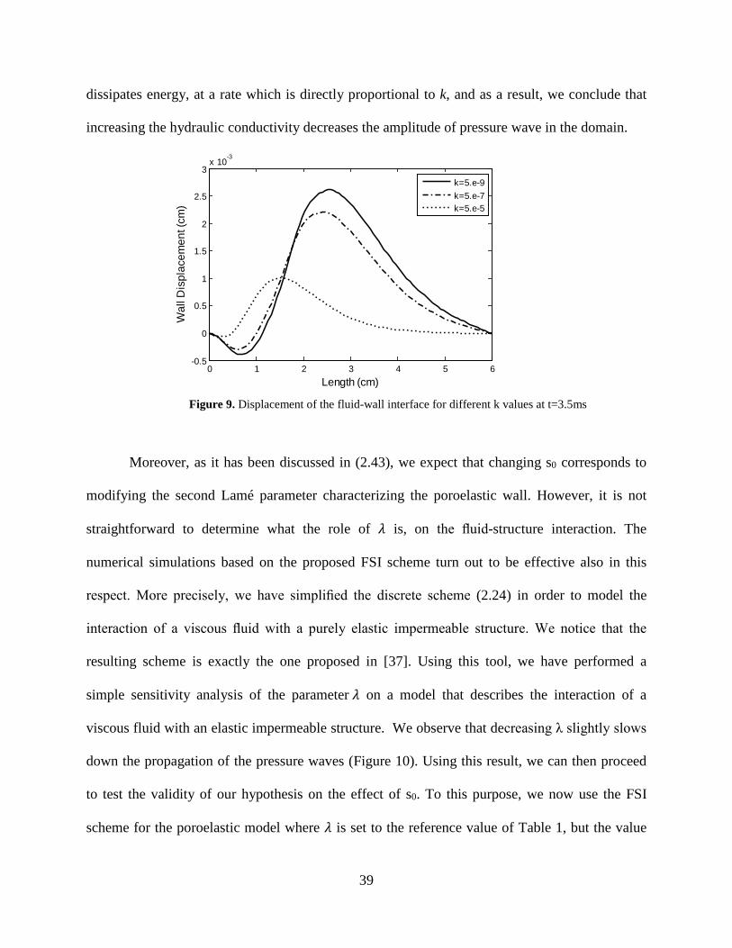
39

dissipates energy, at a rate which is directly proportional to k, and as a result, we conclude that

increasing the hydraulic conductivity decreases the amplitude of pressure wave in the domain.

Figure 9. Displacement of the fluid-wall interface for different k values at t=3.5ms

Moreover, as it has been discussed in (2.43), we expect that changing s0 corresponds to

modifying the second Lamé parameter characterizing the poroelastic wall. However, it is not

straightforward to determine what the role of 𝜆𝜆 is, on the fluid-structure interaction. The

numerical simulations based on the proposed FSI scheme turn out to be effective also in this

respect. More precisely, we have simplified the discrete scheme (2.24) in order to model the

interaction of a viscous fluid with a purely elastic impermeable structure. We notice that the

resulting scheme is exactly the one proposed in [37]. Using this tool, we have performed a

simple sensitivity analysis of the parameter 𝜆𝜆 on a model that describes the interaction of a

viscous fluid with an elastic impermeable structure. We observe that decreasing λ slightly slows

down the propagation of the pressure waves (Figure 10). Using this result, we can then proceed

to test the validity of our hypothesis on the effect of s0. To this purpose, we now use the FSI

scheme for the poroelastic model where 𝜆𝜆 is set to the reference value of Table 1, but the value

0 1 2 3 4 5 6-0.5

0

0.5

1

1.5

2

2.5

3x 10

-3

Length (cm)

Wal

l Dis

plac

emen

t (cm

)

k=5.e-9k=5.e-7k=5.e-5

40

of the mass storativity is varied as s0 = 5×10−7,5×10−6,10−5. The results shown in Figure 11,

shows that increasing s0 has similar effect on wave speed, since it corresponds to decreasing the

second Lame constant. More precisely, increasing s0 from 5×10−6 to 10−5 corresponds to decrease

𝜆𝜆, which in turn slows down the pressure wave propagation. Conversely, decreasing the mass

storativity corresponds to increase the equivalent second Lamé parameter. As a result, the

pressure wave speeds up.

Figure 10. Displacement of the fluid-wall interface at t=3.5ms for λ = 4.28×106 and λ = 4.28×105

Figure 11. Displacement of the fluid-wall interface at t=3.5ms for different values of storativity

41

2.5 SUMMARY

We have studied the interaction of a free fluid with a poroelastic material with the

assumption of having small deformations. After setting appropriate governing equations on

adjacent domains and discussing the corresponding interface conditions, we have considered the

discretization of the problem in the framework of the finite element method. Particular attention

must be devoted to the approximation of the interface conditions, which are non-standard with

respect to the ones that arise in the coupling of homogenous partial differential equations. We

have shown that the Nitsche’s method, used for the weak approximation of boundary and

interface conditions for elliptic or parabolic problems, is appropriate to enforce the interface

constraints in the variational formulation. Since all the interface conditions correspond to

suitable operators in the variational problem, time-lagging allows to split the fully coupled

problem into subproblems, relative to the main governing equations, such as free fluid flow,

Darcy filtration and elastodynamics. Also the resulting loosely coupled problem formulation

turns out to be stable, provided that it is combined with suitable stabilization operators. This

solution approach is very effective from the computational standpoint, but suffers from low

accuracy. In order to merge the computational efficiency of the loosely coupled scheme with the

good accuracy and stability properties of the monolithic formulation, we develop a numerical

solver where the former scheme acts as a preconditioner for the latter. The theory and the

numerical results suggest that this approach is very effective because the loosely coupled scheme

behaves as an optimal preconditioner for the monolithic formulation. This solution algorithm

turns out to be very robust with respect to the characteristic physical parameters of the problem.

Indeed, we have successfully applied it to the analysis of a problem related to blood flow in

arteries as well as to the study of subsurface flow and deformation of a fractured reservoir [27].

42

3.0 ENERGY DISTRIBUTION IN THE COUPLED FSI PROBLEMS

The present chapter analyzes the distribution and dissipation of the energy in the coupling

between the pulsatile flow and a deformable structure. The objective is to determine new criteria,

based on the energy distribution, for the assessment of constitutive models of the structure part in

a fluid-structure interaction framework. A computational model of blood flow and arterial

deformation is used to examine the behavior of different constitutive models of the arterial wall.

In particular, we consider poroelastic and viscoelastic descriptions of the artery. Energy

estimates are derived for each constitutive model of the arterial wall from the weak formulation

of the fluid/solid coupled problem and are applied to assess energy exchange between different

compartments of the model. Two-dimensional numerical experiments are presented to illustrate

the energy distribution within the fluid and solid model compartments. Results highlight the

importance of including both poroelasticity and viscoelasticity in modeling fluid-structure

interaction in large arteries. Our results show that both viscoelastic and poroelastic models for

the arterial walls absorb part of the input energy flowing to the artery, but the underlying

mechanisms are substantially different.

43

3.1 BACKGROUND

A comprehensive understanding of pressure and flow pulse wave propagation in the

cardiovascular system can provide valuable information for clinical diagnosis and treatment.

Computational models of arteries play a significant role in current vascular research as they can

predict properties of the cardiovascular system that cannot be measured in vivo [46]. Moreover,

in vivo measurements of hemodynamic parameters are expensive and limited to easily accessible

arteries. However, due to the complexity of the cardiovascular system, simplifying assumptions

need to be taken into account when studying the interaction between blood flow and vessel wall.

Assuming that the arterial wall is an elastic structure is a common assumption in FSI modeling.

However, arterial walls, like other soft tissues, consist primarily of water [47]. They exhibit both

viscoelastic and poroelastic behavior. In particular, poroelasticity plays an important role in the

regulation of plasma and solute transport across the wall.

Viscoelasticity is the major mechanical characteristic of soft tissue. It accounts for a

combined fluid like (viscous) and solid like (elastic) behavior. Due to its role in physiological

and pathophysiological function of soft tissues, important information can be obtained by using

computational methods that characterize these phenomena and model their underlying

mechanisms. In [48] two different microscopic mechanisms responsible for macroscopic

viscoelastic effects have been considered, one is the intrinsic viscoelasticity of the collagen

matrix and the other is due to the interphase drag between extracellular matrix and fluid phase,

better known as poroelasticity. Considering poroelasticity is important because almost all

biological tissues contain connective tissues and cells surrounded by fluid-filled extracellular

space and both components consist primarily of water [49]. Poroelastic phenomena become

44

crucial when modeling the mass transport in arteries, which is a mechanism that provides

nourishment, removes waste and delivers drugs to the inner layers of large arteries [50].

Earlier numerical models used to predict blood flow are based on rigid geometries [13] in

which only the arterial lumen needs to be reconstructed and discretized, yielding results in a

relatively short time. However, the rigid wall assumption precludes pressure wave propagation

and overestimates the wall shear stress. There exist a variety of methods to include the effects of

the moving wall in computations, the most prevalent being the arbitrary Lagrangian–Eulerian

(ALE) approach. Applications of the ALE to hemodynamics are discussed in [51-53] and

references therein. For example, the work in [14] focuses on developing FSI numerical methods

for the interaction between incompressible fluids and non-linear elastic solids, with application

to the arterial blood flow. The new approach is evaluated on a patient specific abdominal aorta.

The paper proposes that future developments should address extensions to hyperelastic materials

with viscoelasticity, which represent more accurately the behavior of the arterial wall.

Energy distribution in one heart cycle has been studied in the seminal works by Skalak

[54, 55] for pulmonary artery at rest and in exercise conditions. Also, Bertram [56] presented

methods using Womersley’s theory for calculating viscous and viscoelastic energy dissipation as

a function of time for a segment of canine carotid artery in-vivo. However, their work does not

account for the poroelasticity of the arterial wall. Tsaturyan et al. [57] suggested that

extracellular fluid flow dominates the apparent viscoelastic properties of passive cardiac muscle.

The authors claimed that actual tissue viscoelasticity plays a relatively minor role. The dominant

role of poroelasticity in the mechanics of articular cartilage is generally accepted in [57],

constructing a relatively strong case for the same being true for myocardium [49, 58, 59]. In [59]

Taber discussed the viscoelastic type effect due to nonlinear poroelasticity and examined the role

45

of extracellular fluid flow in the apparent viscoelastic behavior of cardiac muscle. In [59]

comparison of theoretical and published experimental results showed that poroelasticity can

account for several measured myocardial features; including the relative insensitivity of the

stress strain curve to loading rate and of the stress relation curve to the muscle stretch. The study

by Taber also compared the experimental and computed hysteresis loops and observed that they

differ significantly, concluding that poroelastic effects alone cannot justify hysteresis. Thus, it

was suggested that both poroelastic and viscoelastic effects must be considered in biomechanical

studies of passive cardiac muscle.

Modeling fluid-structure interaction in porous media is a challenging and

computationally demanding task. The coupling between a fluid and a single layer poroelastic

structure has been previously studied in [4, 33]. In particular, the work in [4] develops a

computational model of the interaction between an incompressible, Newtonian fluid, described

using the Navier-Stokes equations, and a poroelastic structure modeled as a Biot system. The

problem was solved using both a monolithic and a partitioned approach. In [35] a new

partitioned strategy for the solution of coupled Navier-Stokes and Biot systems is presented. This

approach is based on Nitsche’s method for enforcing fluid/solid interface conditions and

provides an efficient solution method for these complex equations. In [29] the results were

extended to idealized 3D models of arteries, such as straight and bent cylinders.

Experimental measurements of arterial wall indicate that arteries exhibit a viscoelastic

behavior [60, 61]. Canic et al. [17, 62] modeled blood flow in compliant artery using linear

viscoelastic membrane equations to model mechanical properties of arterial walls and compared

theoretical results obtained from Kelvin-Voigt model with experimental results in Armentano et

al. [16]; however those results were obtained under the assumption that the model is one

46

dimensional. Bukac et al. [63] extended the work of [17, 62] by presenting a two dimensional

model capturing the radial and longitudinal displacement of the linearly viscoelastic Koiter shell

for the underlying fluid structure interaction problem. The results were comparable with the

monolithic scheme proposed in [64] as well as viscoelastic model in [65]. In particular, the effect

of aging on the phase difference between the pressure and flow-rate waveforms in the carotid

artery was studied in [65].

In the present work we pursue two general objectives. Firstly, we develop a

computational model of pulsatile blood flow in large arteries that embraces different constitutive

models for the arterial wall. In particular, we focus on a poro-viscoelastic description of the

arterial tissue. Secondly, we apply the model to compare poroelastic and viscoelastic behaviors

on the basis of energetic criteria derived from the energy balance of fluid-structure interaction. In

particular, we aim to identify and compare the sources of energy dissipation in the arterial wall.

Determining the nature of this dissipation mechanism is important for understanding how well

viscoelasticity and poroelasticity capture the natural behavior of the artery. More precisely, we

pursue the following quantitative objectives. One is to quantify the dissipative behavior of a

linear viscoelastic model for arterial wall on the fluid structure interaction under pulsatile blood

flow in arteries. The other is to evaluate the role of the extracellular fluid flow in the apparent

viscoelastic behavior of arterial wall.

3.2 FORMULATION

We consider the blood flow in a compliant channel bounded by a thick material representing the

arterial wall, with a two way coupling between the fluid and the structure. We assume that the

47

vessel is sufficiently large so that the non-Newtonian effects can be neglected. The fluid is

modeled as an incompressible, viscous, Newtonian fluid using the Navier-Stokes equations in a

deformable domain 𝛺𝛺𝑓𝑓(𝑡𝑡):


+ 𝜕𝜕. 𝛻𝛻𝜕𝜕� = 𝛻𝛻.𝜎𝜎𝑓𝑓 𝑖𝑖𝑖𝑖 𝛺𝛺𝑓𝑓(𝑡𝑡) (3.1)

𝛻𝛻. 𝜕𝜕 = 0 𝑖𝑖𝑖𝑖 𝛺𝛺𝑓𝑓(𝑡𝑡) (3.2)



dynamic viscosity and the symmetric part of fluid velocity gradient is defined as 𝐷𝐷(𝜕𝜕) = 12

(∇𝜕𝜕 +

∇𝜕𝜕𝑇𝑇).

We model the arterial wall as a thick structure, which accounts for the media and the

adventitia. We consider different constitutive models for the wall: elastic, viscoelastic and

poroelastic. Even though these models will be used separately, for the sake of generality we

present here the description of a poro-visco-elastic arterial wall. We assume that the arterial wall

is incompressible and isotropic. To model the poroelastic properties of the arterial wall, we use

the Biot system [24, 35] that describes the mechanical behavior of a homogeneous and isotropic

elastic skeleton, and connecting pores filled with fluid. We assume that the fluid flow through

the porous medium is modeled using the Darcy equation. Hence; the Biot system for a

poroelastic material consists of the momentum equation for balance of total forces (3.3), Darcy’s

law (3.4) and the storage equation (3.5) for the fluid mass conservation in the pores of the

matrix:

𝜌𝜌𝑠𝑠𝐷𝐷2𝑈𝑈𝐷𝐷𝑡𝑡2

− 𝛻𝛻. �𝜎𝜎𝑆𝑆 − 𝛼𝛼𝑝𝑝𝑝𝑝𝐼𝐼� = 0 𝑖𝑖𝑖𝑖 𝛺𝛺𝑝𝑝(𝑡𝑡) (3.3)

48

𝑘𝑘−1𝑞𝑞 = −𝛻𝛻𝑝𝑝𝑝𝑝 𝑖𝑖𝑖𝑖 𝛺𝛺𝑝𝑝(𝑡𝑡) (3.4)

𝐷𝐷𝐷𝐷𝑡𝑡

�𝑠𝑠0𝑝𝑝𝑝𝑝 + 𝛼𝛼𝛻𝛻.𝑈𝑈� + 𝛻𝛻. 𝑞𝑞 = 0 𝑖𝑖𝑖𝑖 𝛺𝛺𝑝𝑝(𝑡𝑡) (3.5)

In equation (3.4), the relative velocity of the fluid within the porous wall is denoted by 𝑞𝑞

and 𝑝𝑝𝑝𝑝 is the fluid pressure. Hydraulic conductivity of the porous matrix is denoted by k, the

coefficient 𝑠𝑠0 is the storage coefficient, and the Biot-Willis constant α is the pressure-storage

coupling coefficient. In equation (3.5), D/Dt is material derivative, 𝜌𝜌𝑠𝑠 is arterial wall density and

σs denotes the visco-elasticity stress tensor. In the general viscoelastic formulation for the

arterial wall, it is assumed that the stress tensor consists of two parts, 𝜎𝜎𝐸𝐸and 𝜎𝜎𝑣𝑣𝑖𝑖𝑠𝑠𝑣𝑣𝑜𝑜:

𝜎𝜎𝐸𝐸 = 2𝜇𝜇𝑝𝑝𝐷𝐷(𝑈𝑈) + 𝜆𝜆𝑝𝑝𝛻𝛻 ∙ 𝑈𝑈 𝐼𝐼 (3.6)

𝜎𝜎𝑣𝑣𝑖𝑖𝑠𝑠𝑣𝑣𝑜𝑜 = 𝜂𝜂 𝐷𝐷��̇�𝑈� +𝜂𝜂2

(𝛻𝛻 ∙ �̇�𝑈) (3.7)

In (3.6), 𝜎𝜎𝐸𝐸 describes the purely elastic stress that is given by the linear elasticity model,

where λp and μp are the Lame coefficients of the wall. The symmetric part of deformation

gradient for the structure is denoted by D(U). Under the hypothesis of small deformations, we

define 𝐷𝐷(𝑈𝑈) = 12

(∇𝑈𝑈 + ∇𝑈𝑈𝑇𝑇). The second part of the Cauchy stress tensor, namely 𝜎𝜎𝑣𝑣𝑖𝑖𝑠𝑠𝑣𝑣𝑜𝑜,

accounts for the viscoelastic properties of the vessel walls. It is obtained by utilizing a simple

linear viscoelastic model based on the Kelvin-Voigt viscoelasticity model where a dashpot is

arranged in parallel with a spring. We denote �̇�𝑈 = 𝐷𝐷𝐷𝐷 𝐷𝐷𝑜𝑜

. The constitutive model for the

viscoelastic case can be written as ( where variable 𝜂𝜂 is the viscous modulus of the arterial wall:

𝜎𝜎𝑆𝑆 = 𝜎𝜎𝐸𝐸 + 𝜎𝜎𝑣𝑣𝑖𝑖𝑠𝑠𝑣𝑣𝑜𝑜 = 2𝜇𝜇𝑝𝑝𝐷𝐷(𝑈𝑈) + 𝜆𝜆𝑝𝑝𝛻𝛻 ∙ 𝑈𝑈 𝐼𝐼 + 𝜂𝜂 𝐷𝐷��̇�𝑈� +𝜂𝜂2

(𝛻𝛻 ∙ �̇�𝑈) (3.8)

and the poro-visco-elastic stress is defined as:

𝜎𝜎𝑝𝑝 = 𝜎𝜎𝑆𝑆 − 𝛼𝛼𝑝𝑝𝑝𝑝𝐼𝐼 (3.9)

49

With the assumption of axial symmetry, we use the model for the arterial wall in

cylindrical coordinates (r, Ө, z), with z being the distance on the longitudinal axis. The

displacement vector is written in the form of 𝑈𝑈 = [𝑈𝑈𝑟𝑟 ,𝑈𝑈𝜃𝜃,𝑈𝑈𝑧𝑧] and tensor D becomes:

𝐷𝐷(𝑈𝑈) =

⎢⎢⎢⎢⎢⎡

𝜕𝜕𝑈𝑈𝑟𝑟𝜕𝜕𝑟𝑟

012

(𝜕𝜕𝑈𝑈𝑧𝑧𝜕𝜕𝑟𝑟

+𝜕𝜕𝑈𝑈𝑟𝑟𝜕𝜕𝜕𝜕

)

0𝑈𝑈𝑟𝑟𝑟𝑟

0

12

(𝜕𝜕𝑈𝑈𝑧𝑧𝜕𝜕𝑟𝑟

+𝜕𝜕𝑈𝑈𝑟𝑟𝜕𝜕𝜕𝜕

) 0𝜕𝜕𝑈𝑈𝑧𝑧𝜕𝜕𝜕𝜕 ⎥

⎥⎥⎥⎥⎤

(3.10)

At the inlet and outlet boundaries of the fluid domain, we use the Neumann boundary

conditions provided in (3.11) and (3.12) using values of static pressure:

𝜎𝜎𝑓𝑓𝑖𝑖𝑓𝑓 = −𝑝𝑝𝑖𝑖𝑖𝑖(𝑡𝑡)𝑖𝑖𝑓𝑓 on Γ𝑓𝑓𝑖𝑖𝑖𝑖 × (0,𝑇𝑇) (3.11)

𝜎𝜎𝑓𝑓𝑖𝑖𝑓𝑓 = −𝑝𝑝𝑜𝑜𝑜𝑜𝑜𝑜(𝑡𝑡)𝑖𝑖𝑓𝑓 on Γ𝑓𝑓𝑜𝑜𝑜𝑜𝑜𝑜 × (0,𝑇𝑇) (3.12)

The challenges of the numerical discretization of FSI problems in hemodynamics are

associated with the added-mass effect and the high nonlinearity of the problem [66]. In the case

when the structure is poroelastic, one encounters an additional difficulty due to the fluid-porous

media coupling.

The Biot system is coupled to the fluid by prescribing coupling conditions at the interface

Γ. In particular, we impose the continuity of the velocity and of the normal stress at the interface

via the kinematic (no-slip and conservation of mass) and dynamic (conservation of momentum)

interface conditions. Denoting by 𝑖𝑖𝑓𝑓 the outward normal to the fluid domain and by 𝑡𝑡𝑓𝑓 the

corresponding tangential vector, the coupling conditions read as follows:

𝜕𝜕. 𝑡𝑡𝑓𝑓 =𝐷𝐷𝑈𝑈𝐷𝐷𝑡𝑡

. 𝑡𝑡𝑓𝑓 𝑜𝑜𝑖𝑖 𝛤𝛤(𝑡𝑡) (3.13)

𝜕𝜕.𝑖𝑖𝑓𝑓 = �𝐷𝐷𝑈𝑈𝐷𝐷𝑡𝑡

+ 𝑞𝑞� .𝑖𝑖𝑓𝑓 𝑜𝑜𝑖𝑖 𝛤𝛤(𝑡𝑡) (3.14)

𝑖𝑖𝑓𝑓 .𝜎𝜎𝑓𝑓 𝑖𝑖𝑓𝑓 = −𝑝𝑝𝑝𝑝 𝑜𝑜𝑖𝑖 𝛤𝛤(𝑡𝑡) (3.15)

50

𝑖𝑖𝑓𝑓 .𝜎𝜎𝑓𝑓 𝑖𝑖𝑓𝑓 − 𝑖𝑖𝑓𝑓 .𝜎𝜎𝑝𝑝𝑖𝑖𝑓𝑓 = 0 𝑜𝑜𝑖𝑖 𝛤𝛤(𝑡𝑡) (3.16)

𝑡𝑡𝑓𝑓 .𝜎𝜎𝑓𝑓 𝑖𝑖𝑓𝑓 − 𝑡𝑡𝑓𝑓 .𝜎𝜎𝑝𝑝𝑖𝑖𝑓𝑓 = 0 𝑜𝑜𝑖𝑖 𝛤𝛤(𝑡𝑡) (3.17)

3.2.1 Energy estimation

In order to obtain the energy estimation, we proceed as in [35, 67, 68]. In particular, for blood

flow, we multiply equations (3.1) and (3.2) by v and, pf, respectively. The energy of the Biot

system is obtained by multiplying equation (3.3) by �̇�𝑈, equation (3.4) by q and equation (3.5) by

𝑝𝑝𝑝𝑝. The algebraic identity (3.18) will be systematically used in the derivations. As a result, we

derive the following energy equality (3.19) for the coupled problem.

�𝑢𝑢Ω

𝑎𝑎𝑜𝑜𝑢𝑢 =12𝑎𝑎𝑜𝑜 ∥ 𝑢𝑢 ∥Ω2 (3.18)

�𝜌𝜌𝑓𝑓2Ω𝑓𝑓(𝑜𝑜)‖𝜕𝜕‖2

��Fluid kinetic energy

+ �12Ω𝑝𝑝(𝑜𝑜)�𝜌𝜌𝑝𝑝��̇�𝑈�

2+ 2 𝜇𝜇𝑝𝑝‖𝐷𝐷(𝑈𝑈)‖2 + 𝜆𝜆𝑝𝑝(∇.𝑈𝑈)2�

��wall kinetic and stored energy

+ � � 2𝜇𝜇𝑓𝑓 ∥ 𝐷𝐷(𝜕𝜕) ∥2Ω𝑓𝑓(𝑠𝑠)

𝑜𝑜

0��viscous dissipation

+ � � 𝜂𝜂 ∥ 𝐷𝐷��̇�𝑈� ∥2Ω𝑝𝑝(𝑠𝑠)

𝑜𝑜

0+ � �

𝜂𝜂2∥ ∇. �̇�𝑈 ∥2

Ω𝑝𝑝(𝑠𝑠)

𝑜𝑜

0��wall dissipation

+ �12Ω𝑝𝑝(𝑜𝑜)�𝑆𝑆0�𝑝𝑝𝑝𝑝�

2�

��poroelastic storage term

+ � � 𝑘𝑘−1 ∥ 𝑞𝑞 ∥2Ω𝑝𝑝(𝑠𝑠)

𝑜𝑜

0��intramural flow energy

= 𝐸𝐸𝑓𝑓(0)��fluid initial energy

+ 𝐸𝐸𝑠𝑠(0)��wall initial energy

−� � 𝑝𝑝𝑖𝑖𝑖𝑖𝛤𝛤𝑓𝑓𝑖𝑖𝑖𝑖

(𝑡𝑡) 𝜕𝜕 ⋅ 𝑖𝑖𝑓𝑓𝑜𝑜

0− � � 𝑝𝑝𝑜𝑜𝑜𝑜𝑜𝑜

𝛤𝛤𝑓𝑓𝑜𝑜𝑜𝑜𝑜𝑜

(𝑡𝑡) 𝜕𝜕 ⋅ 𝑖𝑖𝑓𝑓 𝑜𝑜

0��net power of input pressure wave

+ � −� � 𝜌𝜌𝑓𝑓𝛤𝛤𝑓𝑓𝑖𝑖𝑖𝑖

∥ 𝜕𝜕 ∥2

2 𝜕𝜕 ⋅ 𝑖𝑖𝑓𝑓

𝑜𝑜

0− � � 𝜌𝜌𝑓𝑓


∥ 𝜕𝜕 ∥2

2 𝜕𝜕 ⋅ 𝑖𝑖𝑓𝑓

𝑜𝑜

0�

��kinetic energy exchange with the exterior

(3.19)

51

Where ‖∙‖ denotes the Euclidean norm when applied to a vector or the Frobenius norm

when applied to a tensor.

We define Ef as the fluid kinetic energy and Es as the structure kinetic and stored energy

given by (3.20).

𝐸𝐸𝑓𝑓 = �𝜌𝜌𝑓𝑓2Ω𝑓𝑓(𝑜𝑜)‖𝜕𝜕‖2

𝐸𝐸𝑠𝑠 = �12Ω𝑝𝑝(𝑜𝑜)�𝜌𝜌𝑝𝑝��̇�𝑈�

2+ 2 𝜇𝜇𝑝𝑝‖𝐷𝐷(𝑈𝑈)‖2 + 𝜆𝜆𝑝𝑝(∇.𝑈𝑈)2�

(3.20)

The right hand side of (3.19) represents the kinetic and stored energy of the initial state

and the power of external forces. The left hand side of (3.19) represents the different forms of

the system internal energy. On the left hand side of (3.19), we identify the following expressions,

which define the total energy in the elastic, viscoelastic and poroelastic cases respectively.

𝐸𝐸𝑡𝑡𝑜𝑜𝑡𝑡𝑎𝑎𝐸𝐸𝐸𝐸𝐸𝐸𝑠𝑠𝑠𝑠𝑜𝑜𝑖𝑖𝑣𝑣(𝑡𝑡) = 𝐸𝐸𝑓𝑓(𝑡𝑡) + 𝐸𝐸𝑠𝑠(𝑡𝑡) + � � 2𝜇𝜇𝑓𝑓 ∥ 𝐷𝐷(𝜕𝜕) ∥2Ω𝑓𝑓(𝑠𝑠)

𝑜𝑜

0 (3.21)

𝐸𝐸𝑡𝑡𝑜𝑜𝑡𝑡𝑎𝑎𝐸𝐸𝑣𝑣𝑖𝑖𝑠𝑠𝑣𝑣𝑜𝑜𝑒𝑒𝐸𝐸𝑠𝑠𝑠𝑠𝑜𝑜𝑖𝑖𝑣𝑣(𝑡𝑡)

= 𝐸𝐸𝑡𝑡𝑜𝑜𝑡𝑡𝑎𝑎𝐸𝐸𝐸𝐸𝐸𝐸𝑠𝑠𝑠𝑠𝑜𝑜𝑖𝑖𝑣𝑣(𝑡𝑡) + � � 𝜂𝜂 ∥ 𝐷𝐷��̇�𝑈� ∥2Ω𝑝𝑝(𝑠𝑠)

𝑜𝑜

0

+ � �𝜂𝜂2∥ ∇. �̇�𝑈 ∥2


𝑜𝑜

0

(3.22)

𝐸𝐸𝑡𝑡𝑜𝑜𝑡𝑡𝑎𝑎𝐸𝐸𝑝𝑝𝑜𝑜𝑟𝑟𝑜𝑜𝑒𝑒𝐸𝐸𝑠𝑠𝑠𝑠𝑜𝑜𝑖𝑖𝑣𝑣(𝑡𝑡)

= 𝐸𝐸𝑡𝑡𝑜𝑜𝑡𝑡𝑎𝑎𝐸𝐸𝐸𝐸𝐸𝐸𝑠𝑠𝑠𝑠𝑜𝑜𝑖𝑖𝑣𝑣(𝑡𝑡) + 𝐸𝐸𝑠𝑠𝑜𝑜𝑜𝑜𝑟𝑟𝑠𝑠𝑔𝑔𝑒𝑒(𝑡𝑡) + � � 𝑘𝑘−1 ∥ 𝑞𝑞 ∥2Ω𝑝𝑝(𝑠𝑠)

𝑜𝑜

0

(3.23)

Where Estorage is the energy stored into the porous matrix because of pore deformation.

𝐸𝐸𝑠𝑠𝑜𝑜𝑜𝑜𝑟𝑟𝑠𝑠𝑔𝑔𝑒𝑒 = �12Ω𝑝𝑝(𝑜𝑜)�𝑆𝑆0�𝑝𝑝𝑝𝑝�

2� (3.24)

52

In the case when a fluid is coupled with an “elastic” structure, (3.21) shows that the only

dissipative mechanism is viscous dissipation of the fluid. For the viscoelastic model we have

additional energy damping due to the viscoelasticity of the wall. For the poroelastic model, in

addition to the dissipation due to the fluid viscosity, another energy exchange mechanism

appears due to the permeability of the porous matrix and corresponding filtration velocity.

Figure 12. Computational approach; (a) poro-viscoelastic model of the arterial wall (left), schematic of the

fluid and structure domains (right); (b) inflow/outflow pressure waves and choice of snapshot times (left);

computational mesh (middle), Coupling conditions in Fluid-poroviscoelastic structure interaction (right).

pore space

solid skeleton

0 0.2 0.4 0.6 0.8 160

80

100

120

Time (second)

Pre

ssur

e (m

mH

g)

PoutPin

Finite element analysis

Analysis of energy flowAnalysis of energy in poroelastic and viscoelastic model

53


We have adopted the partitioned, loosely coupled algorithm that we developed in Section 2.3.1 .

The partitioned solve is based on weak enforcement of interface conditions using Nitsche’s

method , and allows us to independently solve the equations for each problem, at each time step.

Namely, structure mechanics, the intramural filtration and the blood flow problem are solved

separately, once at each time step, denoted with the generic index n. The stability of the

partitioned algorithm is a very delicate question. Stability is guaranteed for our solver thanks to

the introduction of the pressure stabilization operator proposed in [37] and provided that several

penalty parameters are appropriately selected [69]. Here the steps are explained for poroelastic

model. Similar approach for viscoelastic model is performed. The only difference is that steps

1,2,3 are solved when the poroelastic model is adopted; in the elastic and viscoelastic cases only

step 1 (solving for the displacement solely) and 3 are necessary because the arterial wall is

considered to be impermeable.

Step1: We first solve the elastodynamics equation for the structure, where the pressure

term has been time-lagged.

𝜌𝜌𝑝𝑝𝐷𝐷2𝑈𝑈𝐷𝐷𝑡𝑡2

− 𝛻𝛻. �𝜎𝜎𝑠𝑠 − 𝛼𝛼𝑝𝑝𝑝𝑝𝑖𝑖−1𝐼𝐼� = 0 𝑖𝑖𝑖𝑖 𝛺𝛺𝑝𝑝

This equation is complemented with the following Robin-type boundary condition on Γ,

where 𝛾𝛾𝑓𝑓 is a parameter that should be chosen sufficiently large to guarantee stability and it is

inversely proportional to the space discretization mesh characteristic size h,

𝑖𝑖𝑝𝑝𝜎𝜎𝑝𝑝𝑖𝑖𝑝𝑝 = 𝑖𝑖𝑝𝑝𝜎𝜎𝑓𝑓𝑖𝑖−1𝑖𝑖𝑝𝑝 − 𝛾𝛾𝑓𝑓(ℎ−1)𝜇𝜇𝑓𝑓 �𝐷𝐷𝑈𝑈𝐷𝐷𝑡𝑡

− 𝜕𝜕𝑖𝑖−1 + 𝑞𝑞𝑖𝑖−1� . 𝑖𝑖𝑝𝑝

𝑡𝑡𝑝𝑝𝜎𝜎𝑝𝑝𝑖𝑖𝑝𝑝 = 𝑡𝑡𝑝𝑝𝜎𝜎𝑓𝑓𝑖𝑖−1𝑖𝑖𝑝𝑝 − 𝛾𝛾𝑓𝑓(ℎ−1)𝜇𝜇𝑓𝑓 �𝐷𝐷𝑈𝑈𝐷𝐷𝑡𝑡

− 𝜕𝜕𝑖𝑖−1� . 𝑡𝑡𝑝𝑝

(3.25)

54

Step 2: The second problem consists of Darcy equations, Complemented with the

boundary condition (3.26):

𝑘𝑘−1𝑞𝑞 = −𝛻𝛻𝑝𝑝𝑝𝑝 𝑖𝑖𝑖𝑖 𝛺𝛺𝑝𝑝


�𝑠𝑠0𝑝𝑝𝑝𝑝 + 𝛼𝛼𝛻𝛻.𝑈𝑈� + 𝛻𝛻. 𝑞𝑞 = 0 𝑖𝑖𝑖𝑖 𝛺𝛺𝑝𝑝

𝑝𝑝𝑝𝑝 = −𝑖𝑖𝑝𝑝𝜎𝜎𝑓𝑓𝑖𝑖−1𝑖𝑖𝑝𝑝 − 𝛾𝛾𝑓𝑓(ℎ−1)𝜇𝜇𝑓𝑓 �𝜕𝜕𝑖𝑖−1 − �𝐷𝐷𝑈𝑈𝐷𝐷𝑡𝑡

�𝑖𝑖−1

− 𝑞𝑞� .𝑖𝑖𝑝𝑝 (3.26)

Step 3: Finally, the third problem corresponds to the fluid equations:


+ 𝜕𝜕. 𝛻𝛻𝜕𝜕� = 𝛻𝛻.𝜎𝜎𝑓𝑓 𝑖𝑖𝑖𝑖 𝛺𝛺𝑓𝑓

𝛻𝛻. 𝜕𝜕 = 0 𝑖𝑖𝑖𝑖 𝛺𝛺𝑓𝑓

𝜕𝜕.𝑖𝑖𝑓𝑓 = �𝐷𝐷𝑈𝑈𝜕𝜕𝑡𝑡

+ 𝑞𝑞� .𝑖𝑖𝑓𝑓 , 𝜕𝜕. 𝑡𝑡𝑓𝑓 =𝐷𝐷𝑈𝑈𝜕𝜕𝑡𝑡

. 𝑡𝑡𝑓𝑓 𝑜𝑜𝑖𝑖 𝛤𝛤 (3.27)

where the kinematic conditions (26) have been enforced using the classical Nitsche’s

method formulation for the boundary conditions.

The non-linearity in the Navier-Stokes equations due to the convective term has been

linearized using the Picard method, namely, 𝜕𝜕𝑖𝑖+1. 𝛻𝛻𝜕𝜕𝑖𝑖+1 ≈ 𝜕𝜕𝑖𝑖. 𝛻𝛻𝜕𝜕𝑖𝑖+1. Moreover, Streamline

Upwind/Petrov-Galerkin (SUPG) formulation is used to stabilize the convection term [70]. To

minimize the numerical dissipation, we adopt the Newmark scheme for the wall discretization.

The continuity equation for the poroelastic pressure is discretized using the Backward Euler

scheme. For the discretization of the blood flow equations we adopt P2 −P1 approximations for

velocity and pressure, respectively, which ensures inf-sup stability of the scheme. The same

types of spaces are used for the intramural filtration and pressure. In addition, we use P2 finite

elements for the discretization of the structure displacement field.

55


In this section, we perform numerical experiments on the simplified 2D/axial symmetric

problems representing blood-vessel systems. Our aim is to clarify the importance of including

arterial wall poroelastic and viscoelastic behaviors in the vascular FSI. The analysis of

simulations will be performed using the general energy estimation (3.19). Namely, we analyze

the energy exchange between different compartments of the elastic, poroelastic and viscoelastic

model. To illustrate the behavior of the models, we consider two examples. The first test,

corresponds to the benchmark problem that has been used in several works [35, 37, 42] for

testing the results of fluid-structure interaction algorithms for blood flow. The flow is driven by a

pressure wave imposed at the inlet boundary for a short amount of time, which then propagates

through the domain. The viscoelasticity modulus in this problem is small compared to its

physiological value [71]. Choosing viscous modulus in this range allows reasonable wave

propagation in the channel and avoids backflow from inlet boundary. The second test problem

concerns a healthy common carotid artery. Model parameters are centered in the range relevant

to cardiovascular applications. The viscoelasticity coefficient is physiologically reasonable, and

higher than in the previous example. In this example, we show that our computational model

gives rise to physiologically reasonable solutions by comparing our results with experimental

data. In both numerical examples, the initial energy of the fluid and structure is defined to be

zero; namely both are at rest. 𝐸𝐸𝑓𝑓(0) = 𝐸𝐸𝑠𝑠(0) = 0.

56

3.4.1 Benchmark 1: FSI analysis for short pressure wave

Benchmark problem described in detail in Section 2.4.1, is employed. The thick structure

equations are written in cylindrical coordinates to naturally account for the circumferential

strains, and coupled with Cartesian equations for the fluid. Model dimension and physical

parameters for this example are provided in Table 4. The problem domain is discretized with a

mesh of 7200 triangles and the propagation of the pressure wave is analyzed over the time

interval [0, 0.005] sec. The final time is smaller than the time necessary for the pressure wave to

reach the outflow. In this way, the unphysical reflected waves that may originate at the outflow

because of homogeneous Neumann conditions do not pollute the considered results. Also, the

velocity at the outlet remains small for the entire simulation time. For this reason, energy loss to

the exterior is minimized. Figure 13 shows a snapshot of the pressure wave moving along the

channel, together with the contour plot of the radial displacement of the artery. The visualization

clearly shows the coupling between the two domains. More precisely, the pressure wave, travels

from left to right, displacing the thick structure.

Table 4. Physical and numerical parameters for benchmark problem 1

Parameters values Parameters values

Radius (cm) 0.5 Lame coeff. μp (dyne/cm2) 1.07×106

Length (cm) 15 Mass storativity , s0 (cm2/dyne) 5×10-6

Wall thickness (cm) 0.1 Hydraulic conductivity ,k (cm3 s/g) 5×10-9

Wall density(g/cm3 ) 1.1 Biot-Willis constant, 𝛼𝛼 1

Fluid density (g/cm3) 1 𝛾𝛾𝑓𝑓, 𝛾𝛾𝑠𝑠 2500

Dynamic viscosity (poise) 0.035 Viscous modulus 𝜂𝜂 (dyne.s/cm2) 100

Lame coeff . λp (dyne/cm2) 4.28×106 Time step Δt 10-5 sec

57

Figure 13. A snapshot of the pressure wave traveling from left to right coupled with the radial component

of the structure displacement. The legend shows the values for the pressure (bottom scale) and displacement (top

scale)

For this test case, we also compare the results obtained using the proposed FSI scheme

with other results available in literature. In particular we refer to the simulations of [72, 73]

obtained using the data of Table II in [38]. Excellent agreement is observed among the results of

the tree methods, reported in Figure 14. This test serves as verification of the software used for

the simulations and as validation of the method.

Figure 15 shows time evolution of the energy components of the system for elastic,

viscoelastic and poroelastic structures; precisely: 𝐸𝐸𝑓𝑓𝑁𝑁 ,𝐸𝐸𝑠𝑠𝑁𝑁 and 𝐸𝐸𝐸𝐸𝑜𝑜𝑠𝑠𝑠𝑠𝑁𝑁 for 𝑖𝑖 = 1, … ,𝑁𝑁 where N is

the number of time steps. 𝐸𝐸𝐸𝐸𝑜𝑜𝑠𝑠𝑠𝑠 corresponds to the viscous loss in fluid, the loss due to the

viscoelasticity of the arterial wall and the filtration velocity in the poroelastic model. We observe

that the total energy (sum of fluid kinetic energy and elastic kinetic and stored energy, including

viscous energy loss) reaches a constant plateau equal to the total energy input. This indicates that

the mass balance is accurately satisfied.

58

Figure 14. Fluid–structure interface displacement (left panel) and mean pressure (right panel) versus z, at

t= 4, 8, 12 ms, computed with the monolithic scheme by Quaini [73] (time step =e-4; dashed line) and with operator-

splitting scheme [72] (time step=5e-5; dotted line). Our result is plotted using a solid line.

Figure 15. Time evolution of the energy in each component for elastic (top, left), viscoelastic (top, right)

and poroelastic cases with k= 5×10-6 cm3s/g (left) and k= 5×10-9 cm

3s/g (right) in benchmark problem 1.

59

The first plot in Figure 17 shows the available energy distributed in different components

for each poroelastic, viscoelastic and elastic cases at final time t=0.005 sec. The results confirm

that for the pressure impulse problem, characterized by high wall accelerations, viscoelastic

losses dominate. The pressure peak is too short to generate a significant intramural flow. The

percentage of fluid viscous dissipation in all cases is almost the same. The stored energy (Es) in

the elastic case in slightly larger than in the other cases since it has no other way for being

dissipated.

3.4.2 Benchmark 2: FSI analysis under physiological condition

In this case, we apply our scheme to model blood flow under physiological conditions. We

consider blood flow in a 2D straight, uniform channel representing a section of a common

carotid artery, and with the assumption of axial symmetry, we solve for upper half of the domain.

For the inflow and outflow boundary conditions we use physiological pressure waves taken from

[65], assuming that the pressure waveform is periodic. We perform computations for several

cardiac cycles starting from the homogeneous initial conditions, until a time-periodic solution is

achieved. A mesh consisting of 4800 tetrahedral cells was created for the fluid and structure

domains.

Our choice of parameters used in this example falls within the range of physiological

values for blood flow and is reported in Table 5. The wall viscosity constant obtained from [71]

for carotid artery was used for viscoelastic model simulations. This choice of viscoelastic

parameters has also been used in other references [65, 74] and is well within the range of

measured viscous moduli of blood vessels reported in [60]. In order to assess the impact of

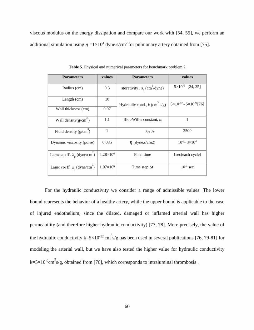
60

viscous modulus on the energy dissipation and compare our work with [54, 55], we perform an

additional simulation using 𝜂𝜂 =1×104 dyne.s/cm2 for pulmonary artery obtained from [75].



Radius (cm) 0.3 storativity , s0 (cm2/dyne) 5×10-6 [24, 35]

Length (cm) 10 Hydraulic cond., k (cm

3 s/g) 5×10-12 - 5×10-9 [76]

Wall thickness (cm) 0.07

Wall density(g/cm3

) 1.1 Biot-Willis constant, 𝛼𝛼 1


Dynamic viscosity (poise) 0.035 𝜂𝜂 (dyne.s/cm2) 104– 3×104

Lame coeff . λp (dyne/cm2) 4.28×106 Final time 1sec(each cycle)

Lame coeff. μp (dyne/cm2) 1.07×106 Time step Δt 10-4 sec

For the hydraulic conductivity we consider a range of admissible values. The lower

bound represents the behavior of a healthy artery, while the upper bound is applicable to the case

of injured endothelium, since the dilated, damaged or inflamed arterial wall has higher

permeability (and therefore higher hydraulic conductivity) [77, 78]. More precisely, the value of

the hydraulic conductivity k=5×10-12 cm3s/g has been used in several publications [76, 79-81] for

modeling the arterial wall, but we have also tested the higher value for hydraulic conductivity

k=5×10-9cm3s/g, obtained from [76], which corresponds to intraluminal thrombosis .

61

3.4.3 Energy balance analysis

Figure 16 shows the distribution of the total input energy of the viscoelastic model in the

second and third cycle, with viscous coefficient 𝜂𝜂=3×104 dyne.s/cm2. The analysis of Figure 16

shows that the periodicity of blood flow is verified, because elastic and kinetic energies initial

and final values at each cycle almost coincide. In addition, it shows that the energy estimate

(3.19) is accurately satisfied in the computations, because the right hand side of (3.19) denoted

by Etot and the total energy input to the system, namely, the left hand side of (3.19) are almost

equivalent. More precisely, energy balance for a periodic cycle states that the net input work

done on the system is equal to the energy losses for each constitutive model. Losses arise from

the action of energy dissipation, due either to blood viscosity, filtration exchange, or wall

viscoelasticity. Namely at the end of each cycle, (3.19) can be written as:

� � 2𝜇𝜇𝑓𝑓 ∥ 𝐷𝐷(𝜕𝜕) ∥2Ω𝑓𝑓(𝑠𝑠)

𝑜𝑜

0+ � � 𝜂𝜂 ∥ 𝐷𝐷��̇�𝑈� ∥2


𝑜𝑜

0+ � �

𝜂𝜂2∥ ∇. �̇�𝑈 ∥2


𝑜𝑜

0

+ � � 𝑘𝑘−1 ∥ 𝑞𝑞 ∥2Ω𝑝𝑝(𝑠𝑠)

𝑜𝑜

0

= −� 𝑝𝑝𝑖𝑖𝑖𝑖𝛤𝛤𝑓𝑓𝑖𝑖𝑖𝑖

(𝑡𝑡) 𝜕𝜕𝑓𝑓 ⋅ 𝑖𝑖𝑓𝑓 − � 𝑝𝑝𝑜𝑜𝑜𝑜𝑜𝑜𝛤𝛤𝑓𝑓𝑖𝑖𝑖𝑖

(𝑡𝑡) 𝜕𝜕𝑓𝑓 ⋅ 𝑖𝑖𝑓𝑓

+ �−� � 𝜌𝜌𝑓𝑓𝛤𝛤𝑓𝑓𝑖𝑖𝑖𝑖

∥ 𝜕𝜕 ∥2

2 𝜕𝜕 ⋅ 𝑖𝑖𝑓𝑓

𝑜𝑜

0− � � 𝜌𝜌𝑓𝑓


∥ 𝜕𝜕 ∥2

2 𝜕𝜕 ⋅ 𝑖𝑖𝑓𝑓

𝑜𝑜

0�

(3.28)

We observe from Figure 16 that, for the viscoelastic model, there is only 2.5%

discrepancy between the left and right hand sides of (3.28). This confirms the accuracy of our

numerical scheme in approximating the energy balance.

62

Figure 16. Time evolution of energy components for viscoelastic case with 𝜼𝜼 =3×104 dyne.s/cm2; The plot

shows kinetic and stored energy in wall (circle), fluid kinetic energy (dash-dot line) , fluid viscous dissipation

(dotted line), wall viscoelastic loss (dashed line), total energy (star), and total input energy to the system (solid line);

for the straight tube (top panel) and stenosed tube (bottom panel)

1 1.5 2 2.5 30

2

4

6

8

10

12x 10

4

Time (s)

Ene

rgy

[erg

]

EfEsEflossEslossEtotEpin/out

1 1.5 2 2.5 30

1

2

3

4

5

6

7

8

9x 10

4

Time (s)

Ene

rgy

[erg

]

EfEsEflossEslossEtotEpin/out

63

Using energy data obtained similarly for elastic and poroelastic model simulations, we

calculate the different energy components for the poroelastic, viscoelastic and elastic cases at

three different times. The choice of the snapshot times is shown in Figure 12. The first time

interval, from [0-0.1] sec, is called systole phase. The second phase, called early diastole, is

between [0.1-0.5] sec, and the last interval, from [0.5-0.9] sec, is called late diastole.

Plots in Figure 17 compare the energy distribution among kinetic energy, stored energy

and losses for the elastic, viscoelastic and poroelastic models at these three snapshot times. The

results in Figure 17 show that at systole all losses are small and the artery behaves nearly as an

elastic structure for all models. The wall elastic energy stored in the arterial walls is the

predominant component of the energy in the system, which drives blood flow during diastole. In

early diastole phase, energy losses in fluid are significant. The viscoelastic loss is small

compared to the flow, while intramural flow is non non-negligible for the higher hydraulic

conductivity value. In the late diastole phase, the dissipation predominates and most of the

energy is dissipated in overcoming the viscous resistance of blood flow. For small permeability

values, we barely notice any contribution related to intramural filtration. We also observe that the

energy dissipated in the wall is a small fraction of that dissipated by the blood. Our results for

predicted energy distribution are coherent to those of [54]. By defining total dissipation as the

sum of fluid the viscous dissipation and the viscoelastic loss at the end of one cycle, our

calculations show that 93% of total dissipation takes place in the in blood flow and only 7% of it

is related to the vascular wall.

64

Figure 17. Available energy at the final time (5ms) in each component for different constitutive models in

benchmark problem 1 (first plot from top); energy distribution at the snapshot times for elastic, viscoelastic

(𝜼𝜼=3×104 dyne.s/cm2) and poroelastic models.

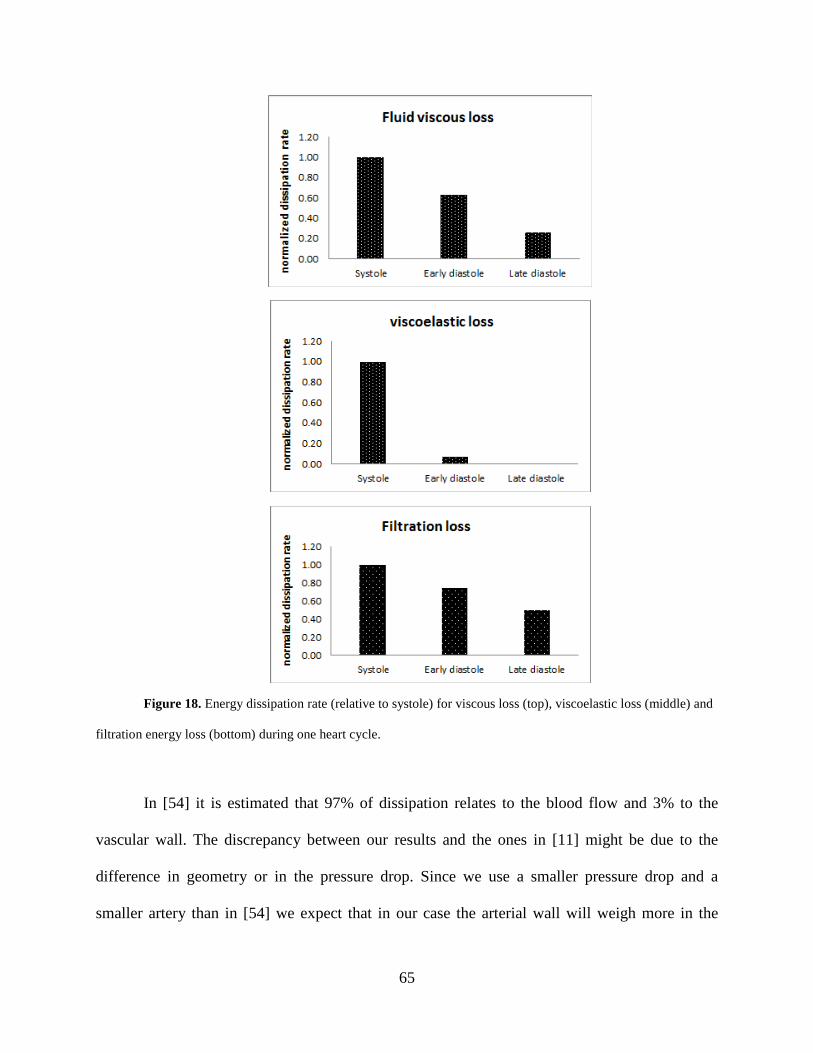
65

Figure 18. Energy dissipation rate (relative to systole) for viscous loss (top), viscoelastic loss (middle) and

filtration energy loss (bottom) during one heart cycle.

In [54] it is estimated that 97% of dissipation relates to the blood flow and 3% to the

vascular wall. The discrepancy between our results and the ones in [11] might be due to the

difference in geometry or in the pressure drop. Since we use a smaller pressure drop and a

smaller artery than in [54] we expect that in our case the arterial wall will weigh more in the

66

energy balance. To validate the robustness of the method with respect to geometries different

than a straight tube, we consider a variation of this benchmark case consisting of a mildly

stenosed artery (see Figure 16 for a representation of the domain). For this case, the results of

simulation for time evolution of energy components is shown in bottom panel of Figure 16. The

similarity of these results with the ones obtained in the case of straight tube suggests that the

conclusions of this work remain qualitatively valid also for more general configurations of the

computational domain.

Starting from the data of Figure 16, we quantify the rates of energy dissipation. Figure 18

informs us about the rate of energy loss in one heartbeat. For each source of energy dissipation

(e.g. viscous dissipation in Figure 18(a), viscoelastic dissipation (b) and intramural filtration (c)),

we define rate of energy loss as the total amount of dissipation over a period of time, divided by

the time interval. Furthermore, we renormalize the dissipation rates by the value obtained in

systole.

In Figure 18 we see that for fluid viscous dissipation rate, the major contribution is in

systole. The contributions of the second and third interval are less significant, because fluid

velocity and velocity gradient are small. Since the highest acceleration of the arterial wall take

place in systole, it plays a key role also in generating viscoelastic loss (middle plot), while the

contributions of two other intervals are almost negligible. The results in Figure 18 (bottom plot)

show that energy flow to intramural filtration is more uniformly distributed among the heartbeat

phases. This behavior can be interpreted observing that the intramural flow energy depends on

the filtration velocity (q), which is more persistent during the cardiac cycle. It should be noted

that in the energy distribution plots the total amount of energy dissipation in systole is the

smallest with respect to the other parts of the heart cycle. The discrepancy between energy

67

dissipation and its rate of variation can be explained observing that the energy dissipation is

cumulative and results from a gradual building up proportional to the total duration of each

phase. As a result, it is lower at systole (the shortest time interval) compared to diastole.

3.4.4 Viscoelastic model analysis

Viscoelasticity causes time lag between pressure wave and arterial wall displacement.

When a cyclically varying stress is applied to a material, the resulting strain stays in phase if the

material is purely elastic. However, if it has viscoelastic properties the strain lags behind the

stress. This lag corresponds to generating a hysteresis loop, which is the indicator of the energy

loss. The area between ascending and descending parts of the loop quantifies the magnitude of

hysteresis and corresponds to the energy dissipation due to the viscous properties of the arterial

wall.

Figure 19 (left panel) shows time lag between normalized pressure and radial

displacement for different values of the wall viscous modulus in the viscoelastic model. The

phase lag is a measure of the amount of viscous damping that takes place in the vessel wall

during each cycle. The viscoelastic effect is also visible in the pressure-displacement relationship

of the arterial wall shown in Figure 19 (right panel). This plot visualizes the hysteresis effects

related to the viscoelastic behavior of the artery. The viscoelastic hysteresis loop obtained by our

numerical simulations is in reasonable quantitative agreement with the published in-vivo data of

the human common carotid artery [65, 74]. To quantify the hysteresis behavior one can calculate

the Energy Dissipation Ratio (EDR), which is a measure of the area inside the pressure-

displacement loop relative to the measure of areas inside and under the loop (see [65] for

details).

68

Figure 19. Time lag in viscoelastic model between normalized pressure in the channel (solid line) and

normalized wall radial displacement (dashed line) at the midpoint of the channel for different values of wall viscous

modulus , 𝜼𝜼 =3×104 dyne.s/cm2 (top), η =1×104 dyne.s/cm2 (middle), and poroelastic model (bottom) are shown in

left panel, corresponding hysteresis plots for each case obtained by plotting the fluid pressure at the center of the

channel versus the radial wall displacement are provided in right panel.

69

Figure 20. Analysis of energy flow (top); Energy diagram in poroelastic and viscoelastic models (bottom)

From the data reported in Figure 19, we calculated wall energy dissipation rate of 9.4%

compared to 8.5% in [74] and 7.8% in [65] for 𝜂𝜂=3×104 dyne.s/cm2, suggesting an slightly

overestimation in our calculated dissipation rate. These effects are compared to the hysteresis of

the poroelastic model (bottom right). Our model suggests that poroelasticity does not generate

any hysteresis, under physiological conditions. On one hand, this analysis confirms that

incorporating the viscoelastic effects into the model is necessary for the accurate representation

of the phase delay between the pressure and radial wall displacement. Moreover, it shows that

walls with higher viscoelasticity have larger hysteresis loop. On the other hand, we observe that

poroelasticity does not introduce any hysteresis effects.

70

3.4.5 Poroelastic Model Analysis

The poroelastic model enables us to study the filtration velocity and therefore coupling

blood flow with mass transport is a potential application of this model. However, we should

consider that for the range of permeability values of healthy arteries, considering intramural

filtration is significant only when we look at the problem over long time scales. Indeed, in

benchmark problem 2 we barely see any effect for poroelasticity when comparing it to the elastic

one. For larger values of permeability, our results confirm that the poroelastic model appreciably

changes the displacement and wave propagation speed in structure as well as the energy

distribution. Figure 15 reports the results of a simulation is performed using k=5×10-6 cm3s/g

which is 1000 times larger than its value provided in Table 4. We observe that increasing

hydraulic conductivity for short time simulation (benchmark problem 1) affects energy

exchange. Our results show that we do not observe hysteresis loops when a poroelastic

constitutive law is applied to the artery. Hysteresis is an outcome of the fact that some part of the

stored energy gets dissipated into a change of natural configuration of the material and cannot be

recovered. Our results confirm that, since for small deformations poroelasticity is a linear model,

it only transforms energy from one kind to another, which is in particular the term related to

intramural flow. Hence, poroelasticity does not contribute to hysteresis in the pressure-diameter

relationship. A sketch of the different behavior of poroelastic and viscoelastic models is shown

in Figure 20. The results by Taber in [59] stated that theoretical hysteresis loop for poroelastic

materials exist, although they are small. However it should be noted that the results in [59] are

based on a nonlinear elasticity formulation for large deformations. Hence, we hypothesize that

large deformations and nonlinear material behavior enhance the effect of poroelasticity. Also

Taber’s results are based on strain dependent permeability. Thus, another possible explanation is

71

that since during large deformation the tissue permeability changes significantly, poroelastic

effects are playing a more relevant role, while at low strain the elastic response dominates.

3.5 SUMMARY

The assumption of negligible viscoelastic and poroelastic response has been routinely made in

the analysis of cardiovascular fluid dynamics. This paper presents fluid–structure interaction

simulations incorporating different constitutive models for vascular tissue to assess the

importance of this simplification. By applying the fluid–structure interaction model to an

idealized (carotid) artery under pulsatile flow, we have demonstrated its capability of predicting

the poroelastic and viscoelastic wall behaviors. The results indicate that in physiological

conditions poroelasticity barely affects the energy distribution of an arterial segment. Since soft

tissues are biphasic materials, with water comprising the majority of the weight, poroelasticity

may be an important mechanism at longer time scales. Poroelasticity cannot reproduce

hysteresis, but it transforms energy of the fluid into intramural flow. Viscoelasticity is

responsible for hysteresis and changes the pressure wave propagation. Being directly derived

from the fundamental laws of flow and energy, the model relies on general foundations and it is

prone to be extended in different directions. For example, we are currently generalizing the

problem formulation based on linear elasticity to finite elasticity, which enables us to account for

large deformations. This improvement will be also combined with the application of patient

specific geometries to this analysis. I extracted this chapter with permission of Springer from the

paper: " computational analysis of energy distribution of coupled blood flow and arterial

deformation ", and my collaborators for this paper were M. Bukac and P. Zunino.

72

4.0 NONLINEAR MODEL FOR FPSI

The main contribution of this chapter is the development of a nonlinear poroelastic structural

model in the context of fluid-porous structure interaction. The general idea is to use this model to

study the influence of different parameters on energy dissipation in a poroelastic medium.

Most of the papers focused on nonlinear elasticity for FSI problems, have used

monolithic scheme for solving FSI system in nonlinear case, with some kinds of preconditioners

[82, 83]. In [82] the authors studied finite elasticity for interaction between blood flow and

elastic arterial wall using a monolithic approach. The design of partitioned algorithms for

uncoupling the solution of the three sub-problems in the interaction between pulsatile flow and

poroelastic material (FPSI) is still partially unexplored. In [84], the authors investigate the FPSI

problem for a viscous fluid and a thick poroelastic structure with small displacement. In our

previous works [8, 27-30] a loosely coupled scheme have been successfully developed and

analyzed for this problem.

To the best of our knowledge, the only previous work in the direction of modeling fluid-

porohyperelastic structure interaction can be found in [5], where the interaction between blood

flow and porohyperelastic arterial model is coupled with mass transport analysis. The present

study attempts to investigate the interaction of blood flow with a porohyperelastic vessel wall

and analyze the role of extracellular fluid flow in the apparent viscoelastic behavior of the

arterial wall. The main novelties are in the design of a Nitsche’s splitting strategy, which

73

separates the fluid from the structure sub-problems for FPSI system undergoing large

deformations, and in the fact that we also study a new benchmark test specifically designed to

investigate the effect of poroelasticity on large deformations.

Many modeling and computational difficulties arise in the numerical simulation of an

incompressible fluid interacting with a poroelastic structure featuring possibly large

deformations. The complex interplay among large solid deformations and fluid flow in a

dynamic setting have been addressed in this study by using porous media theory combined with

advanced computational tool for FSI. We use finite elements for the spatial approximation and

Backward Euler time stepping for time discretization. Since the model is complex, efficiency of

the scheme is a fundamental issue. To reduce the computational cost, the coupled problem is

split among its components and solved using a partitioned approach. We adopt a moving mesh

algorithm, based on Arbitrary Lagrangian Eulerian (ALE) method. There exist a variety of

methods to include the effect of the moving wall in computations, the most prevalent being the

arbitrary Lagrangian–Eulerian (ALE) approach. Applications of ALE method to hemodynamics

are discussed in [51-53] and references therein. Discretization using finite elements leads to a

system of non-linear equations. For this reason, we also discuss the strategy of linearizing such

system of equations by the Newton’s method. In summary, the general objective can be split into

two specific aims: (1) Developing a mathematical model for FPSI with large deformations and

(2) Defining a numerical approximation scheme for the problem at hand.

We use the computational model to perform numerical experiments of FPSI. The

numerical experiments are designed to elucidate the dynamic response of a poroelastic material

under a variety of loading conditions. Our objective is exploring in what condition poroelastic

model is dissipative and examining the range of model parameters that generate a pressure

74

relaxation loop in FPSI. In our previous paper [30] we suggested that poroelastic effects alone

cannot justify hysteresis. More precisely, we observed that poroelasticity does not contribute to

any loop in pressure-diameter relation for small deformation model. However, In [59] Taber

examined the role of extracellular fluid flow in the apparent viscoelastic behavior of cardiac

muscle and results by Taber stated that theoretical hysteresis loop for poroelastic material in

myocardium exists, although they are small. Taber extended the formulation based on

consolidation theory in [85], to study deformation of porous elastic plates and shells saturated

with a viscous fluid, undergoing large axisymmetric deformation. The results in Taber’s paper

are based on finite elasticity formulation for large deformation. So we hypothesize that large

deformation behavior or loading conditions may enhance the effect of poroelasticity.

There is very little information on how energy loss (hysteresis etc.) depends on the rate of

loading or of deformation. The relative contributions of the fluid-solid phase effects

(poroelasticity) and intrinsic solid phase viscoelasticity to this behavior are not known. An

understanding of the nature of these contributions may be used to design implants that behave

more physiologically over a broad range of applied frequencies. One good example is the

intervertebral disc. In [86] , the authors measured the frequency-dependent stiffness and energy

absorption of human lumbar intervertebral discs to determine whether these properties differ due

to fluid-flow dependent behavior.

This chapter is organized as follows. Section 4.1 deals with the description of constitutive

framework for FSI problem at finite strains, namely we first consider the fluid and the structure

as a continuous medium and discuss the governing equations in the fixed configuration. Then we

split the domain into two parts and explore the structure domain in a Lagrangian description by

imposing the conservation laws in the reference configuration and using an arbitrary Lagrangian

75

Eulerian (ALE) formulation to describe the fluid domain. In Section 4.2, the partitioned

algorithm used to solve the fully discrete FSI problem is presented. In Section 4.3, we propose

numerical simulations on two benchmark problems and discuss the relevant numerical results

obtained.

4.1 FORMULATION

We consider a continuous medium, which occupies a moving domain Ω(t) in its current

configuration. It is made of a fluid in motion in the region Ωf(t) and a deformable structure Ωs(t)

and we have 𝛺𝛺𝑓𝑓(𝑡𝑡) ∪ 𝛺𝛺𝑠𝑠(𝑡𝑡) = 𝛺𝛺(𝑡𝑡). The problem consists in finding the time evolution of the

domain and the velocity fields within the fluid and the structure.

Figure 21. Geometric configuration, reference (left) and present (right)

For this purpose, we use the fundamental conservation laws of continuum mechanics

written on the present configuration Ω(t), namely conservation of mass and conservation of

linear momentum. Here in these equations, 𝑈𝑈𝐷𝐷 is the velocity field at any point of the continuum,

∫ 𝜌𝜌𝑏𝑏 𝑎𝑎𝜕𝜕Ω(𝑜𝑜) defines net body forces and ∫ 𝑡𝑡 𝑎𝑎𝑎𝑎∂Ω(𝑜𝑜) is the net surface forces on the surface ∂Ω(𝑡𝑡).

76

We set the following equations for mass and momentum balance:

𝑎𝑎𝑎𝑎𝑡𝑡� 𝜌𝜌 𝑎𝑎𝜕𝜕Ω(𝑜𝑜)

= 0

𝑎𝑎𝑎𝑎𝑡𝑡� 𝜌𝜌𝑈𝑈𝐷𝐷 𝑎𝑎𝜕𝜕Ω(𝑜𝑜)

= � 𝜌𝜌𝑏𝑏 𝑎𝑎𝜕𝜕Ω(𝑜𝑜)

+ � 𝑡𝑡 𝑎𝑎𝑎𝑎∂Ω(𝑜𝑜)

(4.1)

For conservation of momentum it can be written using Cauchy stress definition and

divergence theorem as:

𝑎𝑎𝑎𝑎𝑡𝑡� 𝜌𝜌𝑈𝑈𝐷𝐷 𝑎𝑎𝜕𝜕Ω(𝑜𝑜)

= � 𝜌𝜌𝑏𝑏 𝑎𝑎𝜕𝜕Ω(𝑜𝑜)

+ � 𝛻𝛻. (𝜎𝜎) 𝑎𝑎𝑎𝑎Ω(𝑜𝑜)

If we ignore body forces and by using Reynolds transport theorem:

𝑎𝑎𝑎𝑎𝑡𝑡� 𝑓𝑓 𝑎𝑎𝜕𝜕Ω𝑓𝑓(𝑜𝑜)

= � (𝜕𝜕𝑓𝑓𝜕𝜕𝑡𝑡

+ 𝛻𝛻. (𝑓𝑓𝑈𝑈𝐷𝐷) ) 𝑎𝑎𝜕𝜕Ω𝑓𝑓(𝑜𝑜)

We can write conservation equations as following:

�𝜕𝜕𝜌𝜌𝜕𝜕𝑡𝑡

+ 𝛻𝛻. (𝜌𝜌𝑈𝑈𝐷𝐷) = 0Ω(𝑜𝑜)

�𝜕𝜕𝜌𝜌𝑈𝑈𝐷𝐷𝜕𝜕𝑡𝑡

+ 𝛻𝛻. (𝜌𝜌𝑈𝑈𝐷𝐷⊗ 𝑈𝑈𝐷𝐷) −� 𝛻𝛻.σ = 0Ω(𝑜𝑜)Ω(𝑜𝑜)

(4.2)

Where ⊗ is the tensor product or the dyad of vectors 𝑢𝑢 and 𝜕𝜕 denoted by 𝑢𝑢⊗𝜕𝜕 . Because

of the large displacements, the configuration Ω(t) is time dependent. To overcome this difficulty,

and to evaluate the strain field or write the elastic constitutive laws inside the structure, it is very

convenient to transport the conservation laws on a fixed configuration 𝛺𝛺� . For this purpose, one

must introduce a continuous mapping T which maps any point x0 of the fixed configuration 𝛺𝛺� to

its image x(x0,t) in the present configuration Ω(t). The choice of the configuration 𝛺𝛺0 and the

map T may be arbitrary; hence the name of ALE formulation is given to the resulting equations.

To simplify the calculation, it is advisable to choose a material configuration for the structural

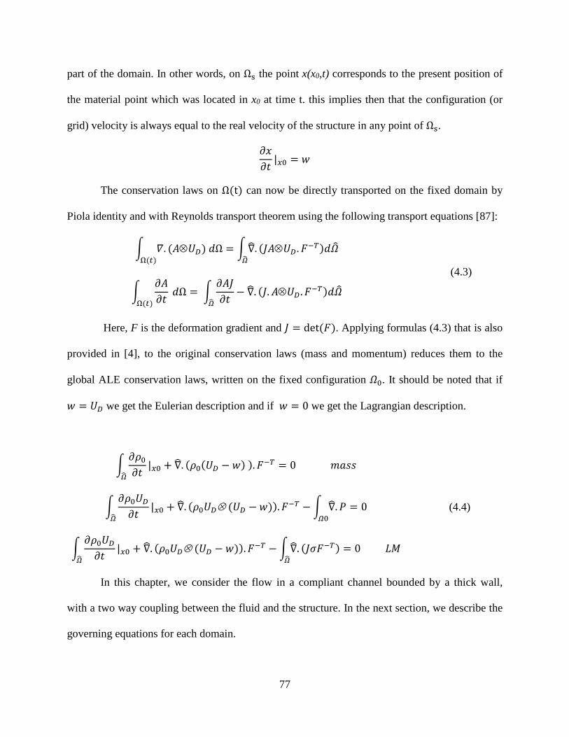
77

part of the domain. In other words, on Ωs the point x(x0,t) corresponds to the present position of

the material point which was located in x0 at time t. this implies then that the configuration (or

grid) velocity is always equal to the real velocity of the structure in any point of Ωs.

𝜕𝜕𝑑𝑑𝜕𝜕𝑡𝑡

|𝑒𝑒0 = 𝑤𝑤

The conservation laws on Ω(t) can now be directly transported on the fixed domain by

Piola identity and with Reynolds transport theorem using the following transport equations [87]:

� 𝛻𝛻. (𝐴𝐴⊗𝑈𝑈𝐷𝐷) 𝑎𝑎ΩΩ(𝑜𝑜)

= �∇�. (𝐽𝐽𝐴𝐴⊗𝑈𝑈𝐷𝐷 .𝐹𝐹−𝑇𝑇)𝑎𝑎𝛺𝛺�𝛺𝛺�

�𝜕𝜕𝐴𝐴𝜕𝜕𝑡𝑡

𝑎𝑎ΩΩ(𝑜𝑜)

= �𝜕𝜕𝐴𝐴𝐽𝐽𝜕𝜕𝑡𝑡

− ∇�. (𝐽𝐽.𝐴𝐴⊗𝑈𝑈𝐷𝐷 .𝐹𝐹−𝑇𝑇)𝑎𝑎𝛺𝛺�𝛺𝛺�

(4.3)

Here, F is the deformation gradient and 𝐽𝐽 = det (𝐹𝐹). Applying formulas (4.3) that is also

provided in [4], to the original conservation laws (mass and momentum) reduces them to the

global ALE conservation laws, written on the fixed configuration 𝛺𝛺0. It should be noted that if

𝑤𝑤 = 𝑈𝑈𝐷𝐷 we get the Eulerian description and if 𝑤𝑤 = 0 we get the Lagrangian description.

�𝜕𝜕𝜌𝜌0𝜕𝜕𝑡𝑡

|𝑒𝑒0 + ∇�. (𝜌𝜌0(𝑈𝑈𝐷𝐷 − 𝑤𝑤) ).𝐹𝐹−𝑇𝑇 = 0 𝑚𝑚𝑎𝑎𝑠𝑠𝑠𝑠𝛺𝛺�

�𝜕𝜕𝜌𝜌0𝑈𝑈𝐷𝐷𝜕𝜕𝑡𝑡

|𝑒𝑒0 + ∇�. (𝜌𝜌0𝑈𝑈𝐷𝐷⊗ (𝑈𝑈𝐷𝐷 − 𝑤𝑤)).𝐹𝐹−𝑇𝑇 − � ∇�.𝑃𝑃 = 0𝛺𝛺0𝛺𝛺�

�𝜕𝜕𝜌𝜌0𝑈𝑈𝐷𝐷𝜕𝜕𝑡𝑡

|𝑒𝑒0 + ∇�. (𝜌𝜌0𝑈𝑈𝐷𝐷⊗ (𝑈𝑈𝐷𝐷 − 𝑤𝑤)).𝐹𝐹−𝑇𝑇 − �∇�. (𝐽𝐽𝜎𝜎𝐹𝐹−𝑇𝑇) = 0 𝐿𝐿𝑀𝑀𝛺𝛺�𝛺𝛺�

(4.4)

In this chapter, we consider the flow in a compliant channel bounded by a thick wall,

with a two way coupling between the fluid and the structure. In the next section, we describe the

governing equations for each domain.

78

4.1.1 Fluid model in the ALE form

We assume that the vessel is sufficiently large so that the non-Newtonian effects can be

neglected. The fluid is modeled as an incompressible, viscous, Newtonian fluid using the Navier-

Stokes equations, i.e., the equations describing conservation of mass and momentum.

�𝜕𝜕𝜌𝜌0𝜕𝜕𝑡𝑡

|𝑒𝑒0 + ∇�. (𝜌𝜌0(𝜕𝜕 − 𝑤𝑤) ).𝐹𝐹−𝑇𝑇 = 0𝛺𝛺�

�𝜕𝜕𝜌𝜌0𝜕𝜕𝜕𝜕𝑡𝑡

|𝑒𝑒0 + ∇�. (𝜌𝜌0𝜕𝜕⊗ (𝜕𝜕 − 𝑤𝑤)).𝐹𝐹−𝑇𝑇 − �∇�. (𝐽𝐽𝜎𝜎𝐹𝐹−𝑇𝑇) = 0𝛺𝛺�𝛺𝛺�

(4.5)

In these expressions it is simpler to compute the partial time derivatives on the fixed

reference configuration and all other stress terms on the present configuration. These equations

are a particular case of the ones presented in section 2.1. They are obtained by replacing 𝑈𝑈𝐷𝐷 by

𝜕𝜕, that denotes here the velocity of the fluid.

We recall that 𝜌𝜌0 = 𝐽𝐽𝜌𝜌𝑓𝑓 ,

Therefore, we can write the first equation in (4.5) as:

�𝜕𝜕𝐽𝐽𝜌𝜌𝑓𝑓𝜕𝜕𝑡𝑡

|𝑒𝑒0 + ∇�. �𝐽𝐽𝜌𝜌𝑓𝑓(𝜕𝜕 − 𝑤𝑤) �.𝐹𝐹−𝑇𝑇 = 0𝛺𝛺�

We compute the partial time derivative on the fixed reference configuration. Using

transport equations (4.3), and since 𝐽𝐽 = 𝑎𝑎𝑑𝑑/𝑎𝑎𝑑𝑑� :


|𝑒𝑒0 + ∇�. �𝐽𝐽𝜌𝜌𝑓𝑓(𝜕𝜕 − 𝑤𝑤) �.𝐹𝐹−𝑇𝑇 =𝛺𝛺�


|𝑒𝑒0𝛺𝛺�

+ �∇�. �𝐽𝐽𝜌𝜌𝑓𝑓(𝜕𝜕 − 𝑤𝑤) �.𝐹𝐹−𝑇𝑇𝛺𝛺�

= �𝜕𝜕𝐽𝐽𝜌𝜌𝑓𝑓𝜕𝜕𝑡𝑡

|𝑒𝑒0𝛺𝛺�

+ � 𝛻𝛻. �𝜌𝜌𝑓𝑓(𝜕𝜕 − 𝑤𝑤) �𝛺𝛺𝑓𝑓(𝑜𝑜)

= � 𝐽𝐽−1𝜕𝜕𝐽𝐽𝜌𝜌𝑓𝑓𝜕𝜕𝑡𝑡

|𝑒𝑒0𝛺𝛺𝑓𝑓(𝑜𝑜)

+ � 𝛻𝛻. �𝜌𝜌𝑓𝑓(𝜕𝜕 − 𝑤𝑤) �𝛺𝛺𝑓𝑓(𝑜𝑜)

79

By applying same procedure to the second equation in (4.5) ,we finally have:

� 𝐽𝐽−1𝜕𝜕𝐽𝐽𝜌𝜌𝑓𝑓𝜕𝜕𝑡𝑡

|𝑒𝑒0 + 𝛻𝛻. �𝜌𝜌𝑓𝑓(𝜕𝜕 − 𝑤𝑤) � = 0𝛺𝛺𝑓𝑓(𝑜𝑜)

� 𝐽𝐽−1𝜕𝜕𝐽𝐽𝜌𝜌𝑓𝑓𝜕𝜕𝜕𝜕𝑡𝑡

|𝑒𝑒0 + 𝛻𝛻. �𝜌𝜌𝑓𝑓𝜕𝜕⊗ (𝜕𝜕 − 𝑤𝑤)� − � 𝛻𝛻. (𝜎𝜎𝑓𝑓) = 0𝛺𝛺𝑓𝑓(𝑜𝑜)𝛺𝛺𝑓𝑓(𝑜𝑜)

(4.6)

Here w is the velocity of the mesh, required to deform the fluid mesh in a way that it

matches structure mesh always. After integration by part, the above ALE formulation of the fluid

problem takes the form of the following PDE:

𝐽𝐽−1𝜕𝜕𝐽𝐽𝜌𝜌𝑓𝑓𝜕𝜕𝜕𝜕𝑡𝑡

|𝑒𝑒0 + 𝛻𝛻. �𝜌𝜌𝑓𝑓𝜕𝜕⊗ (𝜕𝜕 − 𝑤𝑤) − 𝜎𝜎𝑓𝑓� = 0 𝑖𝑖𝑖𝑖 𝛺𝛺𝑓𝑓(𝑡𝑡)

Taking into account mass conservation, one can also reduce this equation to the non-

conservative form. This is the fluid model, namely the Navier-Stokes equation in ALE form, is

written as:


+ (𝜕𝜕 − 𝑤𝑤). 𝛻𝛻𝜕𝜕� = 𝛻𝛻.𝜎𝜎𝑓𝑓 𝑖𝑖𝑖𝑖 𝛺𝛺𝑓𝑓(𝑡𝑡) (4.7)

𝛻𝛻. 𝜕𝜕 = 0 𝑖𝑖𝑖𝑖 𝛺𝛺𝑓𝑓(𝑡𝑡) (4.8)



dynamic viscosity and the symmetric part of fluid velocity gradient is defined as 𝐷𝐷(𝜕𝜕) = 12

(∇𝜕𝜕 +

∇𝜕𝜕𝑇𝑇).

80

4.1.2 Lagrangian formulation of the structure model

Since the fixed configuration 𝛺𝛺� is also the fixed configuration for structure, the structure

velocity is equal to the material velocity on the structure domain and we have �̇�𝑈 = 𝑤𝑤 𝑜𝑜𝑖𝑖 𝛺𝛺�𝑠𝑠

Based on this result, the conservation laws for structure part of the domain simply reduce

to the following:

𝜕𝜕𝜌𝜌0𝜕𝜕𝑡𝑡

|𝑒𝑒0 = 0 𝑜𝑜𝑖𝑖 𝛺𝛺�𝑠𝑠

𝜌𝜌𝑠𝑠𝜕𝜕2𝑈𝑈𝜕𝜕𝑡𝑡2

− ∇� . (𝑃𝑃) = 0 𝑖𝑖𝑖𝑖 𝛺𝛺�𝑠𝑠

Here, 𝜎𝜎 is the Cauchy stress tensor, F is the deformation gradient and “∇�” is the nabla

operator with respect to the material with respect to the material coordinates in the reference

domain. P is the first Piola stress defined as 𝑃𝑃 = 𝐽𝐽𝜎𝜎𝐹𝐹−𝑇𝑇. Using the relationship 𝜎𝜎 = 𝐽𝐽−1𝐹𝐹𝑆𝑆𝐹𝐹𝑇𝑇

between Cauchy stress and 2nd Piola stress tensor S, the model for elastic wall in Lagrangian/

reference configuration 𝛺𝛺�𝑠𝑠 is:


− 𝛻𝛻. (𝐽𝐽𝜎𝜎𝐹𝐹−𝑇𝑇) = 0


− 𝛻𝛻. (𝐽𝐽 (𝐽𝐽−1𝐹𝐹𝑆𝑆𝐹𝐹𝑇𝑇) 𝐹𝐹−𝑇𝑇) = 0


− 𝛻𝛻. (𝐹𝐹𝑆𝑆) = 0 𝑜𝑜𝑖𝑖 𝛺𝛺�𝑠𝑠

We use the St. Venant-Kirchhoff hyperelastic constitutive model for the solid matrix for

which the strain energy function is:

𝑊𝑊 =𝜆𝜆𝑝𝑝2𝑡𝑡𝑟𝑟(𝐸𝐸2) + 𝜇𝜇𝑝𝑝𝐸𝐸:𝐸𝐸 (4.9)

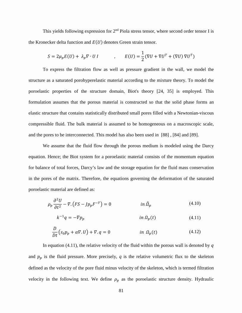
81

This yields following expression for 2nd Piola stress tensor, where second order tensor I is

the Kronecker delta function and 𝐸𝐸(𝑈𝑈) denotes Green strain tensor.

𝑆𝑆 = 2𝜇𝜇𝑝𝑝𝐸𝐸(𝑈𝑈) + 𝜆𝜆𝑝𝑝𝛻𝛻 ∙ 𝑈𝑈 𝐼𝐼 , 𝐸𝐸(𝑈𝑈) =12

(∇𝑈𝑈 + ∇𝑈𝑈𝑇𝑇 + (∇𝑈𝑈) ∇𝑈𝑈𝑇𝑇)

To express the filtration flow as well as pressure gradient in the wall, we model the

structure as a saturated porohyperelastic material according to the mixture theory. To model the

poroelastic properties of the structure domain, Biot's theory [24, 35] is employed. This

formulation assumes that the porous material is constructed so that the solid phase forms an

elastic structure that contains statistically distributed small pores filled with a Newtonian-viscous

compressible fluid. The bulk material is assumed to be homogeneous on a macroscopic scale,

and the pores to be interconnected. This model has also been used in [88] , [84] and [89].

We assume that the fluid flow through the porous medium is modeled using the Darcy

equation. Hence; the Biot system for a poroelastic material consists of the momentum equation

for balance of total forces, Darcy’s law and the storage equation for the fluid mass conservation

in the pores of the matrix. Therefore, the equations governing the deformation of the saturated

poroelastic material are defined as:


− 𝛻𝛻. �𝐹𝐹𝑆𝑆 − 𝐽𝐽𝑝𝑝𝑝𝑝𝐹𝐹−𝑇𝑇� = 0 𝑖𝑖𝑖𝑖 𝛺𝛺�𝑝𝑝 (4.10)

𝑘𝑘−1𝑞𝑞 = −𝛻𝛻𝑝𝑝𝑝𝑝 𝑖𝑖𝑖𝑖 𝛺𝛺𝑝𝑝(𝑡𝑡) (4.11)


�𝑠𝑠0𝑝𝑝𝑝𝑝 + 𝛼𝛼𝛻𝛻.𝑈𝑈� + 𝛻𝛻. 𝑞𝑞 = 0 𝑖𝑖𝑖𝑖 𝛺𝛺𝑝𝑝(𝑡𝑡) (4.12)

In equation (4.11), the relative velocity of the fluid within the porous wall is denoted by 𝑞𝑞

and 𝑝𝑝𝑝𝑝 is the fluid pressure. More precisely, q is the relative volumetric flux to the skeleton

defined as the velocity of the pore fluid minus velocity of the skeleton, which is termed filtration

velocity in the following text. We define 𝜌𝜌𝑝𝑝 as the poroelastic structure density. Hydraulic

82

conductivity of the porous matrix is denoted by k, the coefficient 𝑠𝑠0 is the storage coefficient,

and the Biot-Willis constant α is the pressure-storage coupling coefficient.

We also use a consistent ‘effective stress’ measure for the solid matrix response where

𝜎𝜎𝑆𝑆𝑆𝑆 is the Cauchy stress tensor of the skeleton, and 𝑝𝑝𝑝𝑝 is the mean pore pressure. 𝜎𝜎𝑃𝑃 denotes the

elasticity stress tensor which is defined as 𝜎𝜎𝑃𝑃 = 𝜎𝜎𝑆𝑆𝑆𝑆 − 𝛼𝛼𝑝𝑝𝑝𝑝𝐼𝐼. The Cauchy effective stress tensor

of the skeleton is transformed to the 2nd Piola-Kirchhoff stress tensor S as 𝑆𝑆𝑃𝑃 = 𝑆𝑆𝑆𝑆𝑆𝑆 − 𝐽𝐽𝑝𝑝𝑝𝑝𝐶𝐶−1,

where 𝐶𝐶 = 𝐹𝐹𝑇𝑇𝐹𝐹.

4.1.3 Coupling conditions over the interface

The fluid and poroelastic structure problems must be coupled by imposing three interface

coupling conditions: on velocity, stress, and geometry. Denoting by 𝑖𝑖𝑓𝑓 the outward normal to the

fluid domain and by 𝑡𝑡𝑓𝑓 the corresponding tangential vector, the requirements for compatibility

and the no-slip condition require the following:

𝜕𝜕. 𝑡𝑡𝑓𝑓 =𝐷𝐷𝑈𝑈𝐷𝐷𝑡𝑡

. 𝑡𝑡𝑓𝑓 𝑜𝑜𝑖𝑖 𝛤𝛤(𝑡𝑡) (4.13)

𝜕𝜕.𝑖𝑖𝑓𝑓 = �𝐷𝐷𝑈𝑈𝐷𝐷𝑡𝑡

+ 𝑞𝑞� .𝑖𝑖𝑓𝑓 𝑜𝑜𝑖𝑖 𝛤𝛤(𝑡𝑡) (4.14)

𝑖𝑖𝑓𝑓 .𝜎𝜎𝑓𝑓 𝑖𝑖𝑓𝑓 = −𝑝𝑝𝑝𝑝 𝑜𝑜𝑖𝑖 𝛤𝛤(𝑡𝑡) (4.15)

𝑖𝑖𝑓𝑓 .𝜎𝜎𝑓𝑓 𝑖𝑖𝑓𝑓 − 𝑖𝑖𝑓𝑓 .𝜎𝜎𝑝𝑝𝑖𝑖𝑓𝑓 = 0 𝑜𝑜𝑖𝑖 𝛤𝛤(𝑡𝑡) (4.16)

𝑡𝑡𝑓𝑓 .𝜎𝜎𝑓𝑓 𝑖𝑖𝑓𝑓 − 𝑡𝑡𝑓𝑓 .𝜎𝜎𝑝𝑝𝑖𝑖𝑓𝑓 = 0 𝑜𝑜𝑖𝑖 𝛤𝛤(𝑡𝑡) (4.17)

In Equation (4.13) and (4.14) velocity continuity is enforced across the fluid-solid

interface, in particular equation (4.14) describes the continuity of normal flux over the interface,

which corresponds to the conservation of mass principle. Balance of the normal components of

83

stress in the fluid phase gives Equation (4.15). Moreover, for traction continuity, we need to

ensure the balance of stresses on the interface. Considering continuity of the both normal and

tangential components of stress, is served by conservation of momentum in (4.17) and (4.16).

We also have the kinematic constraint between solid and mesh displacements. It means

the velocity of the mesh is able to deform the fluid mesh in a way that it matches structure mesh

always.

�̇�𝑈 =𝐷𝐷𝑈𝑈𝐷𝐷𝑡𝑡

= 𝑤𝑤 𝑜𝑜𝑖𝑖 𝛤𝛤(𝑡𝑡) (4.18)


For fluid-porous-solid interaction, a two-way coupled model must be used, wherein the

fluid flow and the solid deformations mutually affect each other. A common approach to dealing

with this problem is to separate the two models and solve each one independently by means of an

iterative loop. The two algorithms communicate through the coupling conditions on the interface.

Solving the separated problems serially multiple times is referred to as a “partitioned approach”.

Nitsche’s method has been used for enforcing the interface conditions between non-conforming

meshes in the fluid and structure domains. Formulation of Nitsche’s method for a “FSI only”

system is provided in [37] and has been applied in a similar manner for FPSI system in [27] for

enforcing interface conditions, where the interface conditions (4.13)-(4.17) appear in the

variational formulation in a modular form. Therefore, it is straightforward to design a partitioned

algorithm to solve each equation of the problem independently using time lagging.

84

The use of an ALE formulation for the fluid, together with a Lagrangian frame for the

structure, yields an FPSI problem that is composed by four subproblems, namely the fluid

problem, which allows for the computation of the velocity and pressure inside the fluid domain,

the elasticity problem, which describes the deformation of the vessel wall, the Darcy problem,

which allows for the computation of the velocity and pressure inside the porous medium and the

ALE map update, which accounts for the change in time of the computational fluid domain. The

numerical approach is described below in details.

4.2.1 Spatial discretization using finite elements

The coupled fluid/ poroelastic structure problem consists of finding the solution for the velocity

and pressure field in fluid domain denoted by (𝜕𝜕,𝑝𝑝𝑓𝑓) and also the velocity and pressure field in

the porous media defined by (𝑞𝑞,𝑝𝑝𝑝𝑝) as well as displacement and velocity of the wall (𝑈𝑈, �̇�𝑈). The

finite element method (FEM) was applied to solve the coupled system of equations.

We denote with 𝑉𝑉ℎ𝑓𝑓 ,𝑄𝑄ℎ

𝑓𝑓 the finite element spaces for the velocity and pressure approximation on

the fluid domain Ω𝑓𝑓, with 𝑉𝑉ℎ𝑝𝑝,𝑄𝑄ℎ

𝑝𝑝 the spaces for velocity and pressure approximation of the

porous domain Ω𝑝𝑝 and with 𝑋𝑋ℎ𝑝𝑝, �̇�𝑋ℎ

𝑝𝑝 the approximation spaces for the structure displacement and

velocity, respectively. We assume that all the finite element approximation spaces comply with

the prescribed Dirichlet conditions on external boundaries 𝜕𝜕Ω𝑓𝑓 , 𝜕𝜕Ω𝑝𝑝.

Then we define the bilinear forms for each for each sub-problem. To obtain the bilinear

form for nonlinear elasticity equation, we use the principle of minimum potential energy. The

bilinear form relative to the pure elastic behavior of the structure, namely equation (4.10), is:

85

𝑎𝑎𝑠𝑠(𝑈𝑈ℎ,𝜑𝜑𝑝𝑝,ℎ): = � 𝜑𝜑𝑝𝑝,ℎ�−𝛻𝛻. (𝐹𝐹𝑆𝑆)�𝛺𝛺�𝑝𝑝

= � 𝐹𝐹𝑆𝑆:𝛻𝛻𝜑𝜑𝑝𝑝,ℎ𝛺𝛺�𝑝𝑝

= � (𝐼𝐼 + ∇𝑈𝑈ℎ) 𝑆𝑆:𝛻𝛻𝜑𝜑𝑝𝑝,ℎ𝛺𝛺�𝑝𝑝

= � 𝑆𝑆:𝐷𝐷𝜀𝜀(𝑈𝑈ℎ)[𝜑𝜑𝑝𝑝,ℎ] 𝑎𝑎𝑑𝑑�𝛺𝛺�𝑝𝑝

(4.19)

Where 𝐷𝐷𝜀𝜀(𝑈𝑈ℎ)[𝜑𝜑𝑝𝑝,ℎ] is the Gateaux derivative of 𝜀𝜀 at 𝑈𝑈 in the direction of 𝜑𝜑𝑝𝑝 .

𝐷𝐷𝜀𝜀(𝑈𝑈ℎ)�𝜑𝜑𝑝𝑝,ℎ� = lim𝛥𝛥𝑜𝑜→0

𝜀𝜀�𝑈𝑈ℎ + 𝛥𝛥𝑡𝑡 𝜑𝜑𝑝𝑝,ℎ� − 𝜀𝜀(𝑈𝑈ℎ)𝛥𝛥𝑡𝑡

𝐷𝐷𝜀𝜀(𝑈𝑈ℎ)[𝜑𝜑𝑝𝑝,ℎ] =12

(∇𝜑𝜑𝑝𝑝,ℎ + ∇𝜑𝜑𝑝𝑝,ℎ𝑇𝑇 + ∇𝜑𝜑𝑝𝑝,ℎ ∇𝑈𝑈ℎ𝑇𝑇 + ∇𝑈𝑈ℎ ∇𝜑𝜑𝑝𝑝,ℎ

𝑇𝑇)

(4.20)

Also we also have:

𝑏𝑏𝑠𝑠�𝑝𝑝𝑝𝑝,ℎ,𝜑𝜑𝑝𝑝,ℎ�: = 𝛼𝛼� 𝐽𝐽 𝑝𝑝𝑝𝑝,ℎ𝛺𝛺�𝑝𝑝

𝐹𝐹−𝑇𝑇: (𝛻𝛻𝜑𝜑𝑝𝑝,ℎ)𝑎𝑎𝑑𝑑� (4.21)

For the Darcy problem in a poroelastic medium we have two other terms, which account

for the filtration through the porous matrix, equations (4.11)-(4.12), defined as:

𝑎𝑎𝑝𝑝(𝑞𝑞ℎ, 𝑟𝑟ℎ): = � 𝜅𝜅−1𝛺𝛺𝑝𝑝

𝑞𝑞ℎ ⋅ 𝑟𝑟ℎ𝑎𝑎𝑑𝑑, 𝑏𝑏𝑝𝑝(𝑝𝑝𝑝𝑝,ℎ, 𝑟𝑟ℎ): = � 𝑝𝑝𝑝𝑝,ℎ𝛺𝛺𝑝𝑝

𝛻𝛻 ⋅ 𝑟𝑟ℎ𝑎𝑎𝑑𝑑

For the flow equations (4.7)-(4.8), the trilinear and bilinear forms are:

𝑎𝑎𝑓𝑓�𝜕𝜕ℎ, 𝜕𝜕ℎ,𝜑𝜑𝑓𝑓,ℎ�: = 2𝜇𝜇𝑓𝑓 � 𝐷𝐷Ω𝑓𝑓

(𝜕𝜕ℎ):𝐷𝐷�𝜑𝜑𝑓𝑓,ℎ�𝑎𝑎𝑑𝑑 + 𝜌𝜌𝑓𝑓 � (𝜕𝜕ℎ.𝛻𝛻)𝜕𝜕ℎ ⋅ 𝜑𝜑𝑓𝑓,ℎ𝑎𝑎𝑑𝑑Ω𝑓𝑓

,

𝑏𝑏𝑓𝑓(𝑝𝑝𝑓𝑓,ℎ,𝜑𝜑𝑓𝑓,ℎ): = � 𝑝𝑝𝑓𝑓,ℎΩ𝑓𝑓

𝛻𝛻 ⋅ 𝜑𝜑𝑓𝑓,ℎ𝑎𝑎𝑑𝑑,

The forcing term for boundary conditions is:

𝐹𝐹�𝑡𝑡;𝜑𝜑𝑓𝑓,ℎ� = −� 𝑝𝑝𝑖𝑖𝑖𝑖Γ𝑓𝑓𝑖𝑖𝑖𝑖

(𝑡𝑡) 𝜑𝜑𝑓𝑓,ℎ ⋅ 𝑖𝑖𝑓𝑓

And finally, the following interface terms appear in the variational equations,

𝐼𝐼Γ = �(Γ𝜎𝜎𝑓𝑓,ℎ𝑖𝑖 ⋅ 𝜑𝜑𝑓𝑓,ℎ − 𝜎𝜎𝑝𝑝,ℎ𝑖𝑖 ⋅ 𝜑𝜑𝑝𝑝,ℎ + 𝑝𝑝𝑝𝑝,ℎ𝑟𝑟ℎ ⋅ 𝑖𝑖) (4.22)

86

Starting from the expression of 𝐼𝐼Γ, Nitsche’s method allows us to weakly enforce the

interface conditions (4.13)-(4.17). Details for interface bilinear form can be found in [35]. Based

on the assumption that the solution of the system and the chosen test functions are regular

enough, for any 𝑡𝑡 ∈ (0,𝑇𝑇), we have semi-discrete coupled fluid/solid problem as the following

equation, considering that �̇�𝑈ℎ𝑖𝑖 = 𝑎𝑎𝜏𝜏𝑈𝑈ℎ𝑖𝑖.

𝜌𝜌𝑝𝑝 � 𝑎𝑎𝜏𝜏𝛺𝛺�𝑝𝑝

�̇�𝑈ℎ ⋅ 𝜑𝜑𝑝𝑝,ℎ𝑎𝑎𝑑𝑑� + 𝜌𝜌𝑝𝑝 � (𝛺𝛺�𝑝𝑝

�̇�𝑈ℎ − 𝑎𝑎𝜏𝜏𝑈𝑈ℎ) ⋅ �̇�𝜑𝑝𝑝,ℎ𝑎𝑎𝑑𝑑� + 𝑎𝑎𝑠𝑠�𝑈𝑈ℎ,𝜑𝜑𝑝𝑝,ℎ�

+ 𝜌𝜌𝑓𝑓 � 𝜕𝜕𝑜𝑜Ω𝑓𝑓

𝜕𝜕ℎ ⋅ 𝜑𝜑𝑓𝑓,ℎ𝑎𝑎𝑑𝑑 + 𝑠𝑠0 � 𝐷𝐷𝑜𝑜𝛺𝛺𝑝𝑝

𝑝𝑝𝑝𝑝,ℎ𝜓𝜓𝑝𝑝,ℎ𝑎𝑎𝑑𝑑 − 𝑏𝑏𝑠𝑠(𝑝𝑝𝑝𝑝,ℎ,𝜑𝜑𝑝𝑝,ℎ)

+ 𝑏𝑏𝑠𝑠(𝜓𝜓𝑝𝑝,ℎ,𝐷𝐷𝑜𝑜𝑈𝑈ℎ) + 𝑎𝑎𝑝𝑝(𝑞𝑞ℎ, 𝑟𝑟ℎ) − 𝑏𝑏𝑝𝑝(𝑝𝑝𝑝𝑝,ℎ, 𝑟𝑟ℎ) + 𝑏𝑏𝑝𝑝(𝜓𝜓𝑝𝑝,ℎ, 𝑞𝑞ℎ)

+ 𝑎𝑎𝑓𝑓�𝜕𝜕ℎ, 𝜕𝜕ℎ,𝜑𝜑𝑓𝑓,ℎ� − 𝑏𝑏𝑓𝑓�𝑝𝑝𝑓𝑓,ℎ,𝜑𝜑𝑓𝑓,ℎ� + 𝑏𝑏𝑓𝑓�𝜓𝜓𝑓𝑓,ℎ,𝜕𝜕ℎ� − �(Γ𝜎𝜎𝑓𝑓,ℎ𝑖𝑖

⋅ 𝜑𝜑𝑓𝑓,ℎ − 𝜎𝜎𝑝𝑝,ℎ𝑖𝑖 ⋅ 𝜑𝜑𝑝𝑝,ℎ + 𝑝𝑝𝑝𝑝,ℎ𝑟𝑟ℎ ⋅ 𝑖𝑖) = 𝐹𝐹(𝑡𝑡;𝜑𝜑𝑓𝑓,ℎ)

(4.23)

4.2.2 Time discretization

We now address the time discretization. Let 𝛥𝛥𝑡𝑡 denote the time step, 𝑡𝑡𝑖𝑖 = 𝑖𝑖𝛥𝛥𝑡𝑡, 0 ≤ 𝑖𝑖 ≤

𝑁𝑁, and let the first order (backward) discrete time derivative be defined as:

𝑎𝑎𝜏𝜏𝑈𝑈𝑖𝑖: =𝑈𝑈𝑖𝑖 − 𝑈𝑈𝑖𝑖−1

𝛥𝛥𝑡𝑡.

It should be noted that the difference approximation for time derivative of the wall

velocity is obtained using the common three-point second-derivative approximation for the

uniform time grid:

𝑎𝑎𝜏𝜏�̇�𝑈𝑖𝑖: =𝑈𝑈𝑖𝑖 − 2𝑈𝑈𝑖𝑖−1 + 𝑈𝑈𝑖𝑖−2

𝛥𝛥𝑡𝑡2.

87

Using the Backward Euler (BE) method for the time discretization of both the flow and

the structure problem, the fully discrete coupled fluid-solid problem consists of finding

𝜕𝜕ℎ𝑖𝑖,𝑝𝑝𝑓𝑓,ℎ𝑖𝑖 , 𝑞𝑞ℎ𝑖𝑖,𝑝𝑝𝑝𝑝,ℎ

𝑖𝑖 ∈ 𝑉𝑉ℎ𝑓𝑓 × 𝑄𝑄ℎ


𝑝𝑝 and 𝑈𝑈ℎ𝑖𝑖 ∈ 𝑋𝑋ℎ𝑝𝑝, at each 𝑡𝑡𝑖𝑖, such that for any

𝜑𝜑𝑓𝑓,ℎ,𝜓𝜓𝑓𝑓,ℎ, 𝑟𝑟ℎ,𝜓𝜓𝑝𝑝,ℎ ∈ 𝑉𝑉ℎ𝑓𝑓 × 𝑄𝑄ℎ


𝑝𝑝 and 𝜑𝜑𝑝𝑝,ℎ ∈ 𝑋𝑋ℎ𝑝𝑝 we have,

𝜌𝜌𝑝𝑝𝛥𝛥𝑡𝑡2

� (𝛺𝛺�𝑝𝑝

𝑈𝑈ℎ𝑖𝑖 − 2𝑈𝑈ℎ𝑖𝑖−1 + 𝑈𝑈ℎ𝑖𝑖−2).𝜑𝜑𝑝𝑝,ℎ 𝑎𝑎𝑑𝑑� + 𝑎𝑎𝑠𝑠�𝑈𝑈ℎ𝑖𝑖,𝜑𝜑𝑝𝑝,ℎ� + 𝜌𝜌𝑓𝑓 � 𝜕𝜕𝑜𝑜Ω𝑓𝑓

𝜕𝜕ℎ𝑖𝑖 ⋅ 𝜑𝜑𝑓𝑓,ℎ𝑎𝑎𝑑𝑑

+ 𝑠𝑠0 � 𝐷𝐷𝑜𝑜𝛺𝛺𝑝𝑝

𝑝𝑝𝑝𝑝,ℎ𝑖𝑖 𝜓𝜓𝑝𝑝,ℎ𝑎𝑎𝑑𝑑 − 𝑏𝑏𝑠𝑠(𝑝𝑝𝑝𝑝,ℎ

𝑖𝑖 ,𝜑𝜑𝑝𝑝,ℎ) + 𝑏𝑏𝑠𝑠(𝜓𝜓𝑝𝑝,ℎ,𝐷𝐷𝑜𝑜𝑈𝑈ℎ𝑖𝑖)

+ 𝑎𝑎𝑝𝑝(𝑞𝑞ℎ𝑖𝑖, 𝑟𝑟ℎ) − 𝑏𝑏𝑝𝑝(𝑝𝑝𝑝𝑝,ℎ𝑖𝑖 , 𝑟𝑟ℎ) + 𝑏𝑏𝑝𝑝(𝜓𝜓𝑝𝑝,ℎ,𝑞𝑞ℎ𝑖𝑖) + 𝑎𝑎𝑓𝑓(𝜕𝜕ℎ𝑖𝑖, 𝜕𝜕ℎ𝑖𝑖,𝜑𝜑𝑓𝑓,ℎ)

− 𝑏𝑏𝑓𝑓(𝑝𝑝𝑓𝑓,ℎ𝑖𝑖 ,𝜑𝜑𝑓𝑓,ℎ) + 𝑏𝑏𝑓𝑓(𝜓𝜓𝑓𝑓,ℎ,𝜕𝜕ℎ𝑖𝑖) −�(

Γ𝜎𝜎𝑓𝑓,ℎ𝑖𝑖 𝑖𝑖 ⋅ 𝜑𝜑𝑓𝑓,ℎ − 𝜎𝜎𝑝𝑝,ℎ

𝑖𝑖 𝑖𝑖 ⋅ 𝜑𝜑𝑝𝑝,ℎ

+ 𝑝𝑝𝑝𝑝,ℎ𝑖𝑖 𝑟𝑟ℎ.𝑖𝑖) = 𝐹𝐹(𝑡𝑡;𝜑𝜑𝑓𝑓,ℎ)

(4.24)

Since both the deformation gradient F and the 2nd Piola stress tensor S in the bilinear

form 𝑎𝑎𝑠𝑠 depend on the displacement of the structure U, the finite element discretization leads to a

system of non-linear equations. At each iteration, the coupled FSI problem needs to be

linearized. The linearization is performed iteratively by the Newton method (similar to the

approach used in [90], [7] and [91]).

4.2.3 Structure problem

Given 𝜕𝜕ℎ𝑖𝑖−1,𝑝𝑝𝑓𝑓,ℎ𝑖𝑖−1, 𝑞𝑞ℎ𝑖𝑖−1,𝑝𝑝𝑝𝑝,ℎ

𝑖𝑖−1 find 𝑈𝑈ℎ𝑖𝑖 in 𝛺𝛺�𝑠𝑠 such that (4.25):

It should be noted that by considering the equilibrium of stress over the interface namely

conditions (4.16) and (4.17), we can replace 𝜎𝜎𝑝𝑝 with 𝜎𝜎𝑓𝑓. Therefore, normal stresses computed

88

from the fluid iterate at the previous time step will be used to obtain the structure displacement

from (4.25).



𝑈𝑈ℎ𝑖𝑖 − 2𝑈𝑈ℎ𝑖𝑖−1 + 𝑈𝑈ℎ𝑖𝑖−2).𝜑𝜑𝑝𝑝,ℎ + � 𝑆𝑆�𝜀𝜀(𝑈𝑈ℎ𝑖𝑖)�:𝐷𝐷𝜀𝜀(𝑈𝑈ℎ𝑖𝑖)�𝜑𝜑𝑝𝑝,ℎ�𝛺𝛺�𝑝𝑝

+ � 𝜉𝜉𝛺𝛺�𝑝𝑝

𝑈𝑈ℎ𝑖𝑖 ⋅ 𝜑𝜑𝑝𝑝,ℎ + �𝛾𝛾𝑓𝑓𝛤𝛤�

𝜇𝜇𝑓𝑓ℎ−1𝑎𝑎𝜏𝜏𝑈𝑈ℎ𝑖𝑖 ⋅ 𝑡𝑡𝑝𝑝 𝜑𝜑𝑝𝑝,ℎ ⋅ 𝑡𝑡𝑝𝑝

+ �𝛾𝛾𝑓𝑓𝛤𝛤�

𝜇𝜇𝑓𝑓ℎ−1𝑎𝑎𝜏𝜏𝑈𝑈ℎ𝑖𝑖 ⋅ 𝑖𝑖𝑝𝑝 𝜑𝜑𝑝𝑝,ℎ ⋅ 𝑖𝑖𝑝𝑝 − � 𝐽𝐽𝑠𝑠�𝜎𝜎𝑓𝑓,ℎ𝑖𝑖−1𝐹𝐹�𝑠𝑠

−𝑇𝑇𝑖𝑖𝑝𝑝�𝜑𝜑𝑝𝑝,ℎ�𝛤𝛤�

= 𝑏𝑏𝑠𝑠(𝑝𝑝𝑝𝑝,ℎ𝑖𝑖−1,𝜑𝜑𝑝𝑝,ℎ) + �𝛾𝛾𝑓𝑓

𝛤𝛤�𝜇𝜇𝑓𝑓ℎ−1𝜕𝜕ℎ𝑖𝑖−1 ⋅ 𝑡𝑡𝑝𝑝 𝜑𝜑𝑝𝑝,ℎ ⋅ 𝑡𝑡𝑝𝑝


𝜇𝜇𝑓𝑓ℎ−1(𝜕𝜕ℎ𝑖𝑖−1 − 𝑞𝑞ℎ𝑖𝑖−1) ⋅ 𝑖𝑖𝑝𝑝 𝜑𝜑𝑝𝑝,ℎ ⋅ 𝑖𝑖𝑝𝑝.

(4.25)

This problem is equivalent to solving the elastodynamics equation, where the pressure

term has been time-lagged, complemented with the following Robin-type boundary condition on

the interface:

𝜎𝜎𝑝𝑝𝑖𝑖𝑝𝑝 = 𝜎𝜎𝑓𝑓𝑖𝑖−1𝑖𝑖𝑝𝑝 − 𝛾𝛾𝑓𝑓𝜇𝜇𝑓𝑓ℎ−1 �𝐷𝐷𝑈𝑈𝐷𝐷𝑡𝑡

− 𝜕𝜕𝑖𝑖−1 + 𝑞𝑞𝑖𝑖−1� 𝑜𝑜𝑖𝑖 𝛤𝛤

Or equivalently:

𝐹𝐹�𝑠𝑠𝑆𝑆.𝑁𝑁𝑝𝑝 = 𝐽𝐽𝑠𝑠�𝜎𝜎𝑓𝑓𝑖𝑖−1𝐹𝐹�𝑠𝑠−𝑇𝑇𝑁𝑁𝑝𝑝 − 𝛾𝛾𝑓𝑓(ℎ−1)𝜇𝜇𝑓𝑓 �

𝜕𝜕𝑈𝑈𝜕𝜕𝑡𝑡

− 𝜕𝜕𝑖𝑖−1 + 𝑞𝑞𝑖𝑖−1� 𝑜𝑜𝑖𝑖 𝛤𝛤�

Where 𝑁𝑁𝑝𝑝 is defined as the normal vector to the structure domain in the reference

configuration and, 𝑖𝑖𝑝𝑝 is the equivalent vector in the current configuration.

89

4.2.3.1 Newton’s method

A Newton–Raphson iterative strategy has been adopted here to solve the residual

equation through consistent linearization at each time step. In newton method for solving

nonlinear elasticity, we define residual as R=𝑎𝑎𝑠𝑠�𝑈𝑈,𝜑𝜑𝑝𝑝� − 𝐿𝐿(𝜑𝜑𝑝𝑝) .

𝐽𝐽 ∆𝑈𝑈𝑆𝑆 = −𝑓𝑓(𝑑𝑑𝑆𝑆) 𝑤𝑤ℎ𝑟𝑟𝑟𝑟𝑟𝑟 𝐽𝐽 =𝜕𝜕𝑓𝑓𝑇𝑇

𝜕𝜕𝑑𝑑𝑆𝑆

𝑓𝑓(𝑑𝑑𝑆𝑆) = 𝑎𝑎𝑠𝑠�𝑈𝑈𝑆𝑆,𝜑𝜑𝑝𝑝� − 𝐿𝐿�𝜑𝜑𝑝𝑝�

𝜕𝜕𝑓𝑓𝑇𝑇

𝜕𝜕𝑑𝑑𝑆𝑆 ∆𝑈𝑈𝑆𝑆 = 𝐿𝐿[𝑓𝑓] = 𝑎𝑎∗�𝑈𝑈𝑆𝑆,∆𝑈𝑈𝑆𝑆,𝜑𝜑𝑝𝑝� → 𝑈𝑈𝑆𝑆+1 = 𝑈𝑈𝑆𝑆 − ∆𝑈𝑈𝑆𝑆

Also we denote the linearization of 𝑎𝑎𝑠𝑠�𝑈𝑈,𝜑𝜑𝑝𝑝� as 𝑎𝑎𝑠𝑠∗�𝑈𝑈,∆𝑈𝑈,𝜑𝜑𝑝𝑝�:

𝑎𝑎𝑠𝑠∗�𝑈𝑈,∆𝑈𝑈,𝜑𝜑𝑝𝑝�

= � 𝒞𝒞:𝐷𝐷𝜀𝜀(𝑈𝑈)�𝜑𝜑𝑝𝑝�: 𝐷𝐷𝜀𝜀(𝑈𝑈)[∆𝑈𝑈]𝛺𝛺�𝑝𝑝

+ 𝑆𝑆�𝜀𝜀(𝑈𝑈)�:𝐷𝐷2𝜀𝜀(𝑈𝑈)�𝜑𝜑𝑝𝑝,∆𝑈𝑈�


+ 𝒞𝒞: 𝜀𝜀(𝑈𝑈):𝐷𝐷2𝜀𝜀(𝑈𝑈)�𝜑𝜑𝑝𝑝,∆𝑈𝑈�

(4.26)

The coefficients of the Lagrangian elasticity tensor emerges as:

𝒞𝒞𝑖𝑖𝑖𝑖𝑆𝑆𝐸𝐸 = 𝜆𝜆𝑝𝑝𝛿𝛿𝑖𝑖𝑖𝑖𝛿𝛿𝑆𝑆𝐸𝐸 + 𝜇𝜇𝑝𝑝(𝛿𝛿𝑖𝑖𝑆𝑆𝛿𝛿𝑖𝑖𝐸𝐸 + 𝛿𝛿𝑖𝑖𝐸𝐸𝛿𝛿𝑖𝑖𝑆𝑆)

In the context of hyper elasticity, by defining 𝑊𝑊 as stored energy density function, we

can write:

𝑆𝑆 =𝜕𝜕𝑊𝑊𝜕𝜕𝜀𝜀

𝜋𝜋(𝑢𝑢) = � 𝑊𝑊�𝜀𝜀(𝑈𝑈)�𝛺𝛺�𝑝𝑝

𝐷𝐷𝜋𝜋(𝑈𝑈)[𝜑𝜑𝑝𝑝] = � 𝜕𝜕𝑊𝑊𝜕𝜕𝜀𝜀

:𝐷𝐷𝜀𝜀(𝑈𝑈)[𝜑𝜑𝑝𝑝]𝛺𝛺�𝑝𝑝

(4.27)

90

𝐷𝐷2𝜋𝜋(𝑈𝑈)�𝜑𝜑𝑝𝑝,∆𝑈𝑈�

= � 𝜕𝜕2𝑊𝑊𝜕𝜕𝜀𝜀2

:𝐷𝐷𝜀𝜀(𝑈𝑈)�𝜑𝜑𝑝𝑝�: 𝐷𝐷𝜀𝜀(𝑈𝑈)[∆𝑈𝑈]𝛺𝛺�𝑝𝑝

+ 𝜕𝜕𝑊𝑊𝜕𝜕𝜀𝜀

:𝐷𝐷2𝜀𝜀(𝑈𝑈)�𝜑𝜑𝑝𝑝,∆𝑈𝑈�


+ 𝑆𝑆�𝜀𝜀(𝑈𝑈)�:𝐷𝐷2𝜀𝜀(𝑈𝑈)�𝜑𝜑𝑝𝑝,∆𝑈𝑈�

(4.28)

𝒞𝒞 = �2𝜇𝜇𝑝𝑝 + 𝜆𝜆𝑝𝑝 0 𝜆𝜆𝑝𝑝

0 𝜇𝜇𝑝𝑝 0𝜆𝜆𝑝𝑝 0 2𝜇𝜇𝑝𝑝 + 𝜆𝜆𝑝𝑝

�

𝐷𝐷2𝜀𝜀(𝑈𝑈)�𝜑𝜑𝑝𝑝,∆𝑈𝑈� =12

(∇𝜑𝜑𝑝𝑝 ∇𝑈𝑈𝑇𝑇 + ∇𝑈𝑈 ∇𝜑𝜑𝑝𝑝𝑇𝑇)

𝐷𝐷2𝜀𝜀(𝑈𝑈)�𝜑𝜑𝑝𝑝,∆𝑈𝑈� = 𝐸𝐸𝑖𝑖𝑚𝑚𝛥𝛥𝑜𝑜→0

𝐷𝐷𝜀𝜀(𝑈𝑈 + 𝛥𝛥𝑡𝑡 ∆𝑈𝑈)[𝜑𝜑𝑝𝑝]− 𝐷𝐷𝜀𝜀(𝑈𝑈)[𝜑𝜑𝑝𝑝]𝛥𝛥𝑡𝑡

(4.29)

We solve the solution satisfying:

𝑎𝑎𝑠𝑠∗�𝑈𝑈𝑆𝑆,∆𝑢𝑢𝑆𝑆,𝜑𝜑𝑝𝑝� = 𝑅𝑅(𝑈𝑈𝑆𝑆,𝜑𝜑𝑝𝑝)

Update the displacement 𝑈𝑈𝑆𝑆+1 = 𝑈𝑈𝑆𝑆 − ∆𝑈𝑈𝑆𝑆

Break the loop if ‖∆𝑢𝑢𝑆𝑆‖ ≤ 𝑟𝑟𝑝𝑝𝑠𝑠𝑖𝑖𝐸𝐸𝑜𝑜𝑖𝑖

Therefore, the set of linearized residual equations are written as:

𝑎𝑎∗�𝑈𝑈𝑆𝑆,∆𝑈𝑈𝑆𝑆,𝜑𝜑𝑝𝑝� − 𝑎𝑎�𝑈𝑈,𝜑𝜑𝑝𝑝� + 𝐿𝐿�𝜑𝜑𝑝𝑝� = 0

91


� ∆𝑈𝑈𝑆𝑆 ⋅ 𝜑𝜑𝑝𝑝,ℎ𝛺𝛺�𝑝𝑝

+ � 𝒞𝒞:𝐷𝐷𝜀𝜀�𝑈𝑈ℎ𝑖𝑖𝑆𝑆��𝜑𝜑𝑝𝑝,ℎ�: 𝐷𝐷𝜀𝜀�𝑈𝑈ℎ𝑖𝑖

𝑆𝑆�[∆𝑈𝑈𝑆𝑆]𝛺𝛺�𝑝𝑝

+ � 𝜉𝜉𝛺𝛺�𝑝𝑝

∆𝑈𝑈𝑆𝑆

⋅ 𝜑𝜑𝑝𝑝,ℎ + � 𝑆𝑆 �𝜀𝜀�𝑈𝑈ℎ𝑖𝑖𝑆𝑆�� :𝐷𝐷2𝜀𝜀�𝑈𝑈ℎ𝑖𝑖

𝑆𝑆��𝜑𝜑𝑝𝑝,ℎ,∆𝑈𝑈𝑆𝑆�𝛺𝛺�𝑝𝑝

−𝜌𝜌𝑝𝑝𝛥𝛥𝑡𝑡2


𝑈𝑈ℎ𝑖𝑖𝑆𝑆 − 2𝑈𝑈ℎ𝑖𝑖−1 + 𝑈𝑈ℎ𝑖𝑖−2).𝜑𝜑𝑝𝑝,ℎ − � 𝜉𝜉

𝛺𝛺�𝑝𝑝𝑈𝑈ℎ𝑖𝑖

𝑆𝑆 ⋅ 𝜑𝜑𝑝𝑝,ℎ

− � 𝑆𝑆 �𝜀𝜀�𝑈𝑈ℎ𝑖𝑖𝑆𝑆�� :𝐷𝐷𝜀𝜀�𝑈𝑈ℎ𝑖𝑖

𝑆𝑆�[𝜑𝜑𝑠𝑠]𝛺𝛺�𝑝𝑝

− �𝛾𝛾𝑓𝑓𝛤𝛤�

𝜇𝜇𝑓𝑓ℎ−1𝑎𝑎𝜏𝜏𝑈𝑈ℎ𝑖𝑖𝑆𝑆 ⋅ �𝜑𝜑𝑝𝑝,ℎ�

+ � 𝐽𝐽𝑠𝑠�𝜎𝜎𝑓𝑓,ℎ𝑖𝑖−1𝐹𝐹�𝑠𝑠

−𝑇𝑇𝑖𝑖𝑝𝑝�𝜑𝜑𝑝𝑝,ℎ� + �𝛾𝛾𝑓𝑓𝛤𝛤�

𝜇𝜇𝑓𝑓ℎ−1𝜕𝜕ℎ𝑖𝑖−1 𝜑𝜑𝑝𝑝,ℎ𝛤𝛤�

+ 𝑏𝑏𝑠𝑠�𝑝𝑝𝑝𝑝,ℎ𝑖𝑖−1,𝜑𝜑𝑝𝑝,ℎ� + �𝛾𝛾𝑓𝑓

𝛤𝛤�𝜇𝜇𝑓𝑓ℎ−1𝜕𝜕ℎ𝑖𝑖−1 ⋅ 𝑡𝑡𝑝𝑝 𝜑𝜑𝑝𝑝,ℎ ⋅ 𝑡𝑡𝑝𝑝


𝜇𝜇𝑓𝑓ℎ−1(𝜕𝜕ℎ𝑖𝑖−1 − 𝑞𝑞ℎ𝑖𝑖−1) ⋅ 𝑖𝑖𝑝𝑝 𝜑𝜑𝑝𝑝,ℎ ⋅ 𝑖𝑖𝑝𝑝 = 0

(4.30)

4.2.4 Darcy problem

Given 𝜕𝜕ℎ𝑖𝑖−1,𝑝𝑝𝑓𝑓,ℎ𝑖𝑖−1 and 𝑈𝑈ℎ𝑖𝑖, find 𝑞𝑞ℎ,𝑝𝑝𝑝𝑝,ℎ

𝑖𝑖 in 𝛺𝛺𝑝𝑝 such that:

𝑠𝑠0 � 𝐷𝐷𝑜𝑜𝛺𝛺𝑝𝑝

𝑝𝑝𝑝𝑝,ℎ𝑖𝑖 𝜓𝜓𝑝𝑝,ℎ𝑎𝑎𝑑𝑑 + 𝑎𝑎𝑝𝑝(𝑞𝑞ℎ𝑖𝑖, 𝑟𝑟ℎ) − 𝑏𝑏𝑝𝑝�𝑝𝑝𝑝𝑝,ℎ

𝑖𝑖 , 𝑟𝑟ℎ� + 𝑏𝑏𝑝𝑝�𝜓𝜓𝑝𝑝,ℎ,𝑞𝑞ℎ𝑖𝑖�

+ �𝛾𝛾𝑓𝑓𝛤𝛤

𝜇𝜇𝑓𝑓ℎ−1𝑞𝑞ℎ𝑖𝑖 ⋅ 𝑖𝑖𝑝𝑝 𝑟𝑟ℎ ⋅ 𝑖𝑖𝑝𝑝 + 𝑠𝑠𝑓𝑓,𝑞𝑞�𝑎𝑎𝜏𝜏𝑞𝑞ℎ ⋅ 𝑖𝑖𝑝𝑝, 𝑟𝑟ℎ ⋅ 𝑖𝑖𝑝𝑝�

= −𝑏𝑏𝑠𝑠(𝜓𝜓𝑝𝑝,ℎ,𝐷𝐷𝑜𝑜𝑈𝑈ℎ𝑖𝑖) + �𝛾𝛾𝑓𝑓𝛤𝛤

𝜇𝜇𝑓𝑓ℎ−1(𝜕𝜕ℎ𝑖𝑖−1 − 𝐷𝐷𝑜𝑜𝑈𝑈ℎ𝑖𝑖−1) ⋅ 𝑖𝑖𝑝𝑝 𝑟𝑟ℎ

⋅ 𝑖𝑖𝑝𝑝 + �𝑖𝑖𝑝𝑝𝛤𝛤

⋅ 𝜎𝜎𝑓𝑓,ℎ𝑖𝑖−1𝑖𝑖𝑝𝑝 𝑟𝑟ℎ ⋅ 𝑖𝑖𝑝𝑝.

(4.31)

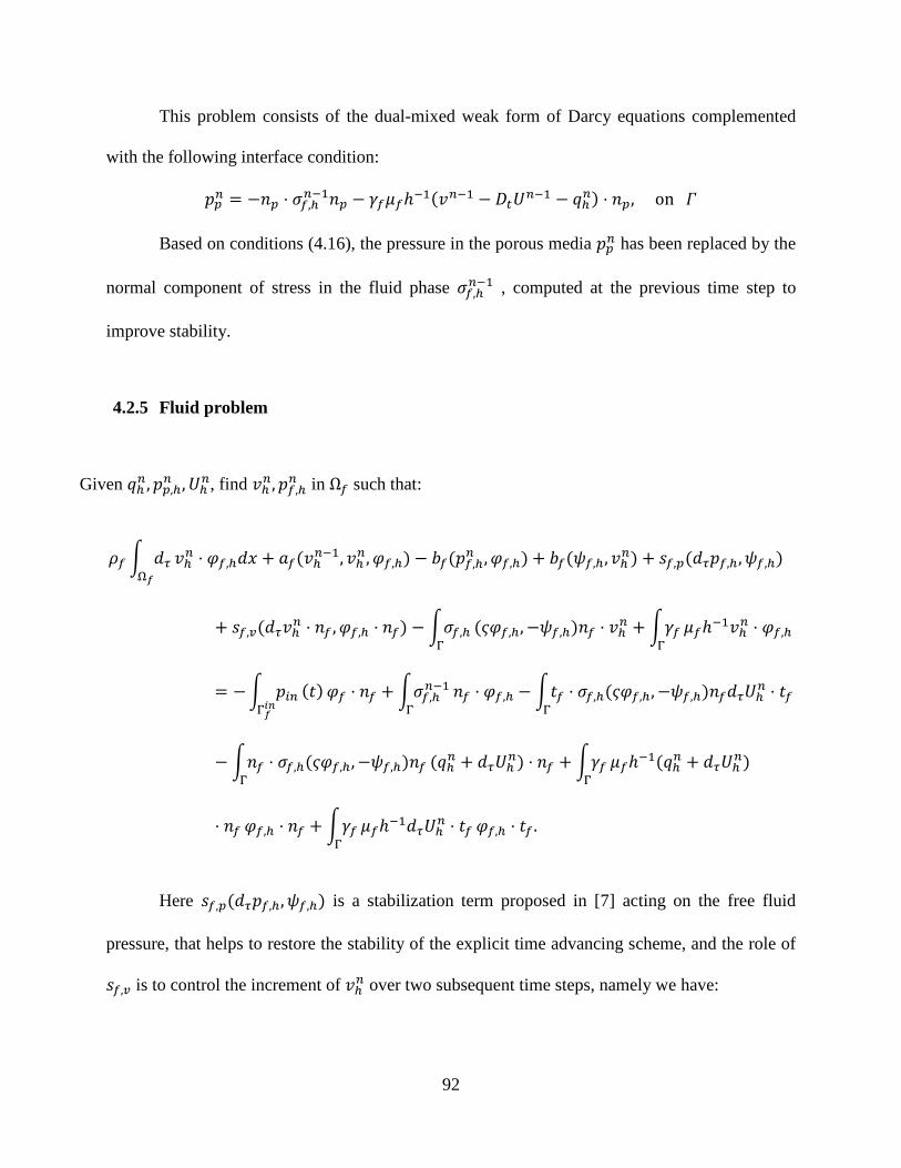
92

This problem consists of the dual-mixed weak form of Darcy equations complemented

with the following interface condition:

𝑝𝑝𝑝𝑝𝑖𝑖 = −𝑖𝑖𝑝𝑝 ⋅ 𝜎𝜎𝑓𝑓,ℎ𝑖𝑖−1𝑖𝑖𝑝𝑝 − 𝛾𝛾𝑓𝑓𝜇𝜇𝑓𝑓ℎ−1(𝜕𝜕𝑖𝑖−1 − 𝐷𝐷𝑜𝑜𝑈𝑈𝑖𝑖−1 − 𝑞𝑞ℎ𝑖𝑖) ⋅ 𝑖𝑖𝑝𝑝, on 𝛤𝛤

Based on conditions (4.16), the pressure in the porous media 𝑝𝑝𝑝𝑝𝑖𝑖 has been replaced by the

normal component of stress in the fluid phase 𝜎𝜎𝑓𝑓,ℎ𝑖𝑖−1 , computed at the previous time step to

improve stability.

4.2.5 Fluid problem

Given 𝑞𝑞ℎ𝑖𝑖,𝑝𝑝𝑝𝑝,ℎ𝑖𝑖 ,𝑈𝑈ℎ𝑖𝑖, find 𝜕𝜕ℎ𝑖𝑖,𝑝𝑝𝑓𝑓,ℎ

𝑖𝑖 in Ω𝑓𝑓 such that:

𝜌𝜌𝑓𝑓 � 𝑎𝑎𝜏𝜏Ω𝑓𝑓

𝜕𝜕ℎ𝑖𝑖 ⋅ 𝜑𝜑𝑓𝑓,ℎ𝑎𝑎𝑑𝑑 + 𝑎𝑎𝑓𝑓(𝜕𝜕ℎ𝑖𝑖−1, 𝜕𝜕ℎ𝑖𝑖,𝜑𝜑𝑓𝑓,ℎ) − 𝑏𝑏𝑓𝑓(𝑝𝑝𝑓𝑓,ℎ𝑖𝑖 ,𝜑𝜑𝑓𝑓,ℎ) + 𝑏𝑏𝑓𝑓(𝜓𝜓𝑓𝑓,ℎ,𝜕𝜕ℎ𝑖𝑖) + 𝑠𝑠𝑓𝑓,𝑝𝑝(𝑎𝑎𝜏𝜏𝑝𝑝𝑓𝑓,ℎ,𝜓𝜓𝑓𝑓,ℎ)

+ 𝑠𝑠𝑓𝑓,𝑣𝑣(𝑎𝑎𝜏𝜏𝜕𝜕ℎ𝑖𝑖 ⋅ 𝑖𝑖𝑓𝑓 ,𝜑𝜑𝑓𝑓,ℎ ⋅ 𝑖𝑖𝑓𝑓) −�𝜎𝜎𝑓𝑓,ℎΓ

(𝜍𝜍𝜑𝜑𝑓𝑓,ℎ,−𝜓𝜓𝑓𝑓,ℎ)𝑖𝑖𝑓𝑓 ⋅ 𝜕𝜕ℎ𝑖𝑖 + �𝛾𝛾𝑓𝑓Γ

𝜇𝜇𝑓𝑓ℎ−1𝜕𝜕ℎ𝑖𝑖 ⋅ 𝜑𝜑𝑓𝑓,ℎ

= −� 𝑝𝑝𝑖𝑖𝑖𝑖Γ𝑓𝑓𝑖𝑖𝑖𝑖

(𝑡𝑡) 𝜑𝜑𝑓𝑓 ⋅ 𝑖𝑖𝑓𝑓 + �𝜎𝜎𝑓𝑓,ℎ𝑖𝑖−1

Γ𝑖𝑖𝑓𝑓 ⋅ 𝜑𝜑𝑓𝑓,ℎ − �𝑡𝑡𝑓𝑓

Γ⋅ 𝜎𝜎𝑓𝑓,ℎ(𝜍𝜍𝜑𝜑𝑓𝑓,ℎ,−𝜓𝜓𝑓𝑓,ℎ)𝑖𝑖𝑓𝑓𝑎𝑎𝜏𝜏𝑈𝑈ℎ𝑖𝑖 ⋅ 𝑡𝑡𝑓𝑓

− �𝑖𝑖𝑓𝑓Γ

⋅ 𝜎𝜎𝑓𝑓,ℎ(𝜍𝜍𝜑𝜑𝑓𝑓,ℎ,−𝜓𝜓𝑓𝑓,ℎ)𝑖𝑖𝑓𝑓 (𝑞𝑞ℎ𝑖𝑖 + 𝑎𝑎𝜏𝜏𝑈𝑈ℎ𝑖𝑖) ⋅ 𝑖𝑖𝑓𝑓 + �𝛾𝛾𝑓𝑓Γ

𝜇𝜇𝑓𝑓ℎ−1(𝑞𝑞ℎ𝑖𝑖 + 𝑎𝑎𝜏𝜏𝑈𝑈ℎ𝑖𝑖)

⋅ 𝑖𝑖𝑓𝑓 𝜑𝜑𝑓𝑓,ℎ ⋅ 𝑖𝑖𝑓𝑓 + �𝛾𝛾𝑓𝑓Γ

𝜇𝜇𝑓𝑓ℎ−1𝑎𝑎𝜏𝜏𝑈𝑈ℎ𝑖𝑖 ⋅ 𝑡𝑡𝑓𝑓 𝜑𝜑𝑓𝑓,ℎ ⋅ 𝑡𝑡𝑓𝑓 .

Here 𝑠𝑠𝑓𝑓,𝑝𝑝(𝑎𝑎𝜏𝜏𝑝𝑝𝑓𝑓,ℎ,𝜓𝜓𝑓𝑓,ℎ) is a stabilization term proposed in [7] acting on the free fluid

pressure, that helps to restore the stability of the explicit time advancing scheme, and the role of

𝑠𝑠𝑓𝑓,𝑣𝑣 is to control the increment of 𝜕𝜕ℎ𝑖𝑖 over two subsequent time steps, namely we have:

93

𝑠𝑠𝑓𝑓,𝑝𝑝(𝑎𝑎𝜏𝜏𝑝𝑝𝑓𝑓,ℎ,𝜓𝜓𝑓𝑓,ℎ): = 𝛾𝛾𝑠𝑠𝑜𝑜𝑠𝑠𝑠𝑠ℎ𝛥𝛥𝑡𝑡𝛾𝛾𝑓𝑓𝜇𝜇𝑓𝑓

�𝑎𝑎𝜏𝜏Γ

𝑝𝑝𝑓𝑓,ℎ𝑖𝑖 𝜓𝜓𝑓𝑓,ℎ (4.32)

𝑠𝑠𝑓𝑓,𝑣𝑣(𝑎𝑎𝜏𝜏𝜕𝜕ℎ𝑖𝑖 ⋅ 𝑖𝑖,𝜑𝜑𝑓𝑓,ℎ ⋅ 𝑖𝑖) = 𝛾𝛾𝑠𝑠𝑜𝑜𝑠𝑠𝑠𝑠′ 𝛾𝛾𝑓𝑓𝜇𝜇𝑓𝑓𝛥𝛥𝑡𝑡ℎ�𝑎𝑎𝜏𝜏Γ

𝜕𝜕ℎ𝑖𝑖 ⋅ 𝑖𝑖𝜑𝜑𝑓𝑓,ℎ ⋅ 𝑖𝑖 (4.33)

4.2.6 Mesh movement

Knowing the displacement of the structure interface, classical harmonic extension

approach has been proposed to update the fluid mesh in fluid–structure interaction problem.

Harmonic extension is explained in [92].

We employ solving diffusion of the interface displacements into the mesh by solving the

Laplace equation for each component of the node position in the undeformed configuration 𝛺𝛺�𝑓𝑓.

Where w is the mesh deformation velocity from the original position and γ is a variable diffusion

coefficient [6]. The idea is to harmonically expand the evolution of the boundary onto the whole

of 𝛺𝛺�𝑓𝑓. Here basically the fluid field is taken as solution of a homogeneous Laplace problem with

boundary conditions imposed by the real solid displacement.

∇. (𝛾𝛾∇𝑤𝑤) = 0 𝑖𝑖𝑖𝑖 𝛺𝛺�𝑓𝑓 (4.34)

It is common to consider diffusion coefficient as a constant [9]. In the numerical tests of

this chapter, we assume γ=1 and we solve for (4.35):

𝛻𝛻2𝑤𝑤 = 0 𝑖𝑖𝑖𝑖 𝛺𝛺�𝑓𝑓

𝑤𝑤.𝑖𝑖 = 0 𝑜𝑜𝑖𝑖 𝜕𝜕𝛺𝛺�𝑓𝑓\ 𝛤𝛤� , Γ�𝑓𝑓𝑖𝑖𝑖𝑖 𝑎𝑎𝑖𝑖𝑎𝑎 Γ�𝑓𝑓𝑜𝑜𝑜𝑜𝑜𝑜

𝑤𝑤 = 𝑎𝑎𝑈𝑈/𝑎𝑎𝑡𝑡 𝑜𝑜𝑖𝑖 𝛤𝛤� = 𝛺𝛺�𝑓𝑓 ∩ 𝛺𝛺�𝑝𝑝

(4.35)

94

Remark: what is the role of γ? With the Laplacian method, mesh lines cross and negative

volumes occur so the problem cannot be completed. To fix this problem, several authors have

proposed a modification to the Laplace method in which a variable diffusivity is introduced [5].

Near the interface the diffusivity is increased making the mesh stiffer. It was found that

increasing the diffusivity as the inverse of the square of the mesh length scale was the most

effective method.


In this section we discuss some numerical experiments aiming at supporting the FPSI algorithm

addressed in the previous section. We have implemented the mathematical methods previously

described into a numerical solver. For the spatial approximation of the fluid and structure

equations we exploit the finite element method. In order to achieve a stable discretization of the

divergence- free constraint, we use inf-sup stable mixed finite elements, i.e. P2-P1

approximation of the velocity and pressure fields, respectively. The system of algebraic

equations arising from the finite element method is solved by means of a direct method, which is

convenient since the number of degrees of freedom is not exceedingly large. In the stopping

criterion for the Newton’s method, tolerance of 1e-5 is adopted. For the time discretization, we

use Backward Euler finite difference method. Due to the fast dynamics of the solution and semi-

explicit treatment of the fluid convective term (𝜕𝜕𝑖𝑖+1. 𝛻𝛻𝜕𝜕𝑖𝑖+1 ≈ 𝜕𝜕𝑖𝑖. 𝛻𝛻𝜕𝜕𝑖𝑖+1), we have to use

very small time step ( ∆𝑡𝑡=1.e-5 sec, is used). All computations have been performed using an in

house finite element solver written in Freefem++ [41]. For stabilization, the SUPG method is

employed [70], discussed also in [93] .

95

We perform numerical experiments on the idealized geometries that can represent blood-

tissue systems. Benchmark problem 1 shows the ability of our proposed methodology to capture

large deformations in the FPSI problem and is motived by FSI problems between blood flow and

the arterial walls. Next, the proposed methodology is used in benchmark problem 2 to study

energy dissipation in the FPSI framework. The geometrical model in this example can resemble

2D model of the left ventricle (LV), similar to the presented LV model in [94] .

4.3.1 Benchmark 1: FSI analysis of pulsatile flow in a compliant channel

Our first test case is a variant of the 2D benchmark problem for the flow in a straight tube

presented in detail in Section 2.4.1.

In order to assess the impact of extending the study to finite elasticity we have performed

two simulations, using hyperelastic model and linear elasticity model for the elastic skeleton of

the porous media in the arterial wall. More precisely, in one simulation we simplify the Green

strain tensor to its linear part as 𝐸𝐸(𝑈𝑈) = 12

(𝛻𝛻𝑈𝑈 + 𝛻𝛻𝑈𝑈𝑇𝑇) for the structure; and the second one we

use the complete Green strain tensor , 𝐸𝐸(𝑈𝑈) = 12

(∇𝑈𝑈 + ∇𝑈𝑈𝑇𝑇 + (∇𝑈𝑈) ∇𝑈𝑈𝑇𝑇). For each model

(linear and nonlinear) we study the propagation of a single pressure wave following pressure

profile, with 2 different values for Pmax ; one using reference value for Pmax = 13334 dyne/cm2

which generates small deformation in the structure called the “weak” wave, and the other one

using 10 × Pmax that can produce large deformation in the wall.

𝑝𝑝𝑖𝑖𝑖𝑖(𝑡𝑡) = �𝑝𝑝𝑚𝑚𝑠𝑠𝑒𝑒

2�1 − cos �

2𝜋𝜋𝑡𝑡𝑇𝑇𝑚𝑚𝑠𝑠𝑒𝑒

�� 𝑖𝑖𝑓𝑓 𝑡𝑡 ≤ 𝑇𝑇𝑚𝑚𝑠𝑠𝑒𝑒

0 𝑖𝑖𝑓𝑓 𝑡𝑡 > 𝑇𝑇𝑚𝑚𝑠𝑠𝑒𝑒 (4.36)

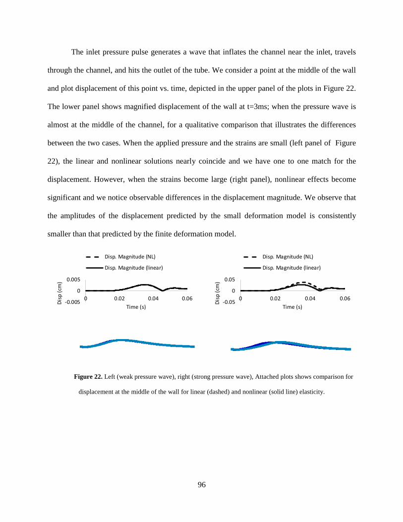
96

The inlet pressure pulse generates a wave that inflates the channel near the inlet, travels

through the channel, and hits the outlet of the tube. We consider a point at the middle of the wall

and plot displacement of this point vs. time, depicted in the upper panel of the plots in Figure 22.

The lower panel shows magnified displacement of the wall at t=3ms; when the pressure wave is

almost at the middle of the channel, for a qualitative comparison that illustrates the differences

between the two cases. When the applied pressure and the strains are small (left panel of Figure

22), the linear and nonlinear solutions nearly coincide and we have one to one match for the

displacement. However, when the strains become large (right panel), nonlinear effects become

significant and we notice observable differences in the displacement magnitude. We observe that

the amplitudes of the displacement predicted by the small deformation model is consistently

smaller than that predicted by the finite deformation model.

Figure 22. Left (weak pressure wave), right (strong pressure wave), Attached plots shows comparison for

displacement at the middle of the wall for linear (dashed) and nonlinear (solid line) elasticity.

-0.005

0

0.005

0 0.02 0.04 0.06

Disp

(cm

)

Time (s)

Disp. Magnitude (NL)

Disp. Magnitude (linear)

-0.05

0

0.05

0 0.02 0.04 0.06

Disp

(cm

)

Time (s)

Disp. Magnitude (NL)

Disp. Magnitude (linear)

97

4.3.2 Benchmark 2: FSI analysis of the flow in a cross-section model

In this example the dynamical behavior of a poroelastic material subjected to a time

dependent loading from the fluid, is investigated. We describe new benchmark settings for the

evaluation of the energy loss in FPSI problems. We consider the problem of injecting an

incompressible fluid in a poroelastic medium with a uniform cross-section, which results in

expansion of the structure. We identify the area occupied by the fluid region, and the structure

region as depicted in Figure 23. The cross section is considered to be a circular sector made of

nonlinear, poroelastic, isotropic, and nearly incompressible material with the following

dimensions: inner radius Ri, outer radius equal to Ro. The fluid and structure regions are

separated by an interface. The geometry dimensions are provided in Table 6.

Figure 23. Schematic of the geometrical model for benchmark problem 2.

A source term g will be considered in (4.38) to model the injection. This injection phase

is needed in order to inflate/deflate the geometry.


+ 𝜕𝜕. 𝛻𝛻𝜕𝜕� = 𝛻𝛻.𝜎𝜎𝑓𝑓 𝑖𝑖𝑖𝑖 𝛺𝛺𝑓𝑓(𝑡𝑡) (4.37)

𝛻𝛻. 𝜕𝜕 = g 𝑖𝑖𝑖𝑖 𝛺𝛺𝑓𝑓(𝑡𝑡) (4.38)

𝑞𝑞

98

The flow is driven by the injection of the fluid into a circle (2D) that represents the fluid

domain. Then fluid is drained out of the media. All presented simulations in this part have been

performed using a sine-type source term with the amplitude of 30 𝑠𝑠−1. We choose a simple sine

function according to:

𝑔𝑔(𝑡𝑡) = 𝑔𝑔𝑚𝑚𝑠𝑠𝑒𝑒 �sin �𝜋𝜋𝑡𝑡𝑇𝑇𝑚𝑚𝑠𝑠𝑒𝑒

�� 𝑖𝑖𝑓𝑓 𝑡𝑡 ≤ 𝑇𝑇𝑚𝑚𝑠𝑠𝑒𝑒 (4.39)

𝑔𝑔𝑚𝑚𝑠𝑠𝑒𝑒 = 30 𝑠𝑠−1 𝑇𝑇𝑚𝑚𝑠𝑠𝑒𝑒 = 0.003 𝑠𝑠 𝑄𝑄(𝑡𝑡) = 𝐴𝐴𝑟𝑟𝑟𝑟𝑎𝑎(𝑡𝑡) × 𝑔𝑔(𝑡𝑡) → 𝑔𝑔 =𝑄𝑄(𝑡𝑡)

𝐴𝐴𝑟𝑟𝑟𝑟𝑎𝑎(𝑡𝑡)



Ri (cm) 0.5 Lame coeff. μp (dyne/cm2) 1.07×106

Ro (cm) 0.4 Lame coeff . λp (dyne/cm2) 4.28×106

wall thickness (cm) 0.1 k (cm3 s/g) 5×10-9

wall density(g/cm3

) 1.1 s0 (cm

2/dyne) 5×10-6


Dynamic viscosity (poise) 0.035 Final time 6ms

The formulation also accounts for detailed variations in fluid pressure and flow across the

thickness. Plots in Figure 25 show the filtration velocity and porous media pressure through the

thickness of the wall, due to steadily increasing internal pressure. Since fluid pressure is

constrained to be zero at the outer radial surface, Darcy pressure starts from zero at exterior and

reaches its maximum at interior (inside channel), as expected.

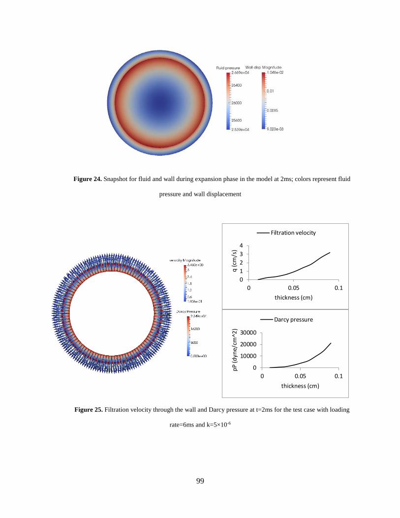
99

Figure 24. Snapshot for fluid and wall during expansion phase in the model at 2ms; colors represent fluid

pressure and wall displacement

Figure 25. Filtration velocity through the wall and Darcy pressure at t=2ms for the test case with loading

rate=6ms and k=5×10-6

01234

0 0.05 0.1

q (c

m/s

)

thickness (cm)

Filtration velocity

0

10000

20000

30000

0 0.05 0.1

pP (d

yne/

cm^2

)

thickness (cm)

Darcy pressure

100

In order to determine the optimal mesh size to use, a mesh sensitivity analysis has been

carried out on the 2D cross sectional model. We solved several test cases with different mesh

sizes of the structure using the reference values provided in Table 6.

Figure 26. Hysteresis loop for different mesh size (left), Schematic of the measuring indicator used in the

sensitivity analysis (right)

Table 7. Mesh sensitivity results

# of cell in 𝛺𝛺𝑠𝑠 Pf × 104 (dyne/cm2) Time step size Pf × 104 (dyne/cm2)

Mesh 1 1788 2.40 ∆t 2.48

Mesh 2 3992 2.48 ∆t/2 2.49

Mesh 3 9194 2.51

We compared the difference in the hysteresis loop between the three different mesh sizes

presented in the left panel of Figure 26. To this purpose, we define an indicator as the pressure in

the loading curve at 0.01 cm value for the displacement (right panel of Figure 26). The results

are provided in Table 7 and Figure 27. The mesh sensitivity analysis shows that after Mesh2

results are almost insensitive to increasing the number of nodes. For this reason, we conclude

0

10000

20000

30000

40000

50000

-0.01 0 0.01 0.02

fluid

pre

ssur

e (d

yne/

cm^2

)

wall disp (cm)

Mesh1 Mesh2 Mesh3

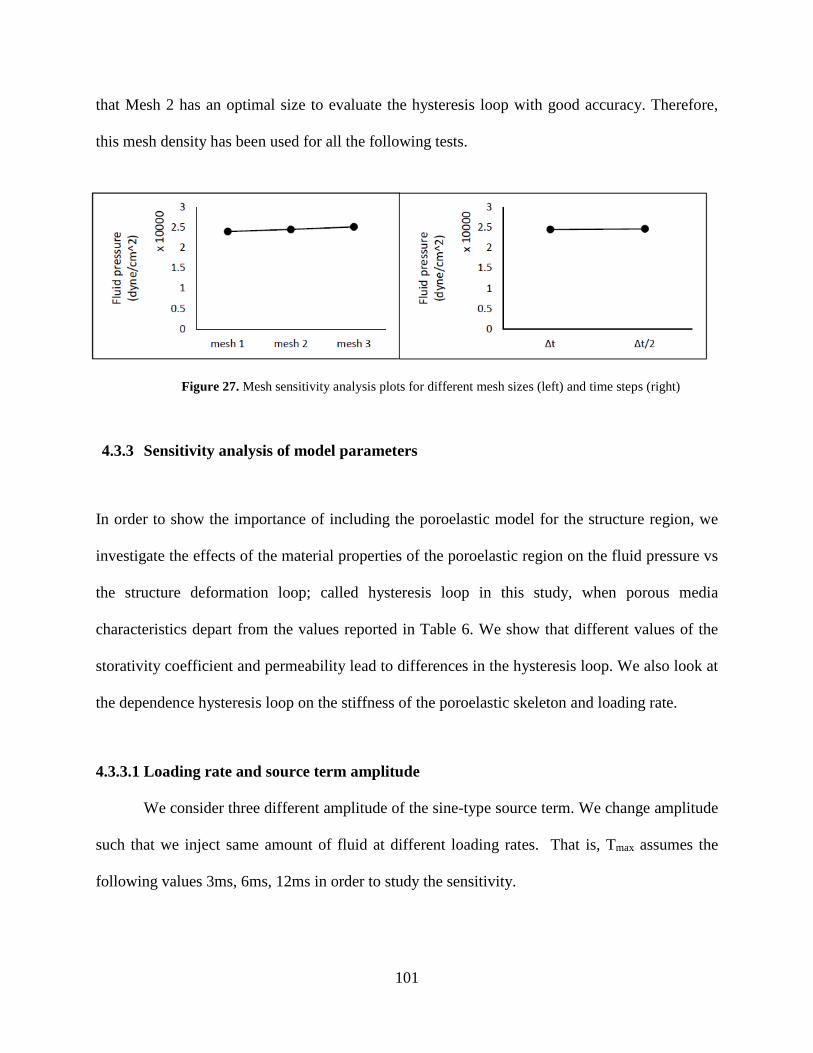
101

that Mesh 2 has an optimal size to evaluate the hysteresis loop with good accuracy. Therefore,

this mesh density has been used for all the following tests.

Figure 27. Mesh sensitivity analysis plots for different mesh sizes (left) and time steps (right)

4.3.3 Sensitivity analysis of model parameters

In order to show the importance of including the poroelastic model for the structure region, we

investigate the effects of the material properties of the poroelastic region on the fluid pressure vs

the structure deformation loop; called hysteresis loop in this study, when porous media

characteristics depart from the values reported in Table 6. We show that different values of the

storativity coefficient and permeability lead to differences in the hysteresis loop. We also look at

the dependence hysteresis loop on the stiffness of the poroelastic skeleton and loading rate.

4.3.3.1 Loading rate and source term amplitude

We consider three different amplitude of the sine-type source term. We change amplitude

such that we inject same amount of fluid at different loading rates. That is, Tmax assumes the

following values 3ms, 6ms, 12ms in order to study the sensitivity.

102

Figure 28. Different source terms g

In Figure 29 and Figure 30, the hysteresis loop for different loading rate values and

different amplitudes of the source term are analyzed. In these simulations the hydraulic

conductivity has been set to the value of k=5×10-6. We observe that the fluid pressure dissipates

more in the high loading regime i.e by increasing g the size of hysteresis loop increases

significantly.

Figure 29. Comparing loops for different values of loading rate, with k=5e-6

Figure 31 shows the comparison of the fluid and Darcy pressure as well as the

displacement and filtration velocity vectors obtained in different loading rate regimes. In the case

of high loading rate (3ms), plots in Figure 31 show that time variation of Darcy pressure, namely

dPp/dt, is bigger and so there exists large pore pressure gradient (dPp/dx) from the beginning as

103

well. Hence, the filtration velocity can attain high velocity quickly; as thus the energy loss occurs

much quicker than small loading rate (12 ms) due to the rapid fluid flow. When there is small

pressure gradient (dPp/dx), the filtration fluid flow (q) is not able to achieve a high velocity in

the short time due to the high damping.

Figure 30. Comparing hysteresis loop for different values of the source term g

Figure 31. Comparing fluid pressure, wall displacement, Darcy pressure and filtration velocity for different

values of loading rate, 3ms (dashed), 6ms (dotted), and 12ms (solid) lines

104

4.3.3.2 Young’s modulus

We investigate the influence of Young’s modulus E on the pressure relaxation loop. We

use k=5×10-6 and the loading rate of 6ms for these simulations. Then, we study the behavior of

the system when we increase and decrease the Young modulus 10 times from its reference value.

Figure 32. Comparing hysteresis loop for different values of Young’s modulus

Figure 33. Comparing fluid pressure, wall displacement, Darcy pressure and filtration velocity for different

values of Young’s modulus,𝟎𝟎.𝟏𝟏 × 𝑬𝑬 (dashed), 𝑬𝑬 (dotted), and 𝟏𝟏𝟎𝟎 × 𝑬𝑬 (solid) lines

-4

1

6

0 0.002 0.004 0.006

Flui

d pr

essu

re X

100

00

(dyn

e/cm

^2)

Time (s) -0.005

0

0.005

0.01

0.015

0.02

0 0.002 0.004 0.006Wal

l dis

plac

emen

t (cm

)

Time (s)

-4

1

6

0 0.004

Darc

y pr

essu

re X

100

00

(dyn

e/cm

^2)

Time (s) -8

-3

2

7

0 0.002 0.004 0.006

Filtr

atio

n ve

loci

ty

(cm

/s)

Time (s)

105

In Figure 32, we analyze the effect of changing Young modulus of the elastic skeleton on

energy dissipation. For the same simulations, pressure values in the fluid and porous media as

well as velocity and displacement fields are shown in Figure 33. Results clearly show that for

very stiff material, the intramural flow squeezes out so hard and quick that the material behaves

as in a single phase elastic material.

4.3.3.3 Storage coefficient

To complete the description of elastic response under fluid infiltration, we also need to

specify how the storage of fluid within material elements changes due to stressing and

pressurization. We assume full saturation of all connected pore space. We observe that changing

the storativity coefficient, which is related to the compressibility of the poroelastic system,

causes a significant difference in the hysteresis loop.in other words, increasing s0 leads to

increase in the fluid mass content by changing the porosity and pressure, which results in more

dissipation.

Figure 34. Comparing hysteresis loop for different values of storage coefficient s0

106

4.3.3.4 Hydraulic conductivity

Figure 35 informs us about the sensitivity of hysteresis loop with respect to hydraulic

conductivity. We observe that, as expected; increasing hydraulic conductivity, increases the

dissipation and we have bigger loop.

Figure 35. Comparing hysteresis loop for different values of hydraulic conductivity

The sensitivity analysis of hydraulic conductivity may help to give interpretation of the

mechanical behavior of tissue engineered vascular grafts (TEVGs). These grafts are porous [95]

and in [96] , the hydraulic conductivity of k=10-7 cm2.s/g is considered for the arterial graft

which is in the range of k for our sensitivity study. Using FPSI model is crucial to investigate

how the prosthetic graft behaves in different configurations from implantation (initial time) to

matured artery, as well as in estimating the risk of both mechanical mismatch in the initial stages

and the eventual rupture.

107

-15

-10

-5

0

5

10

15

0 0.002 0.004 0.006

1/s

Time (s)

D/Dt(s0*pP)

div(q)

D/Dt(div(u))

residual

4.4 DISCUSSION

In the benchmark problem 2, after the poroelastic structure expands to attain equilibrium strain,

pore fluid flow arises within the structure. Both the magnitude of the deformation of the material

and the energy loss associated with its deformation are affected by the flow of the viscous fluid

within the structure, that we call filtration velocity. Using our FPSI model, we investigate the

variation of the filtration velocity inside the poroelastic structure. A remarkable feature of the

numerical results is that the velocity field in the porous matrix has a large variation in the radial

direction. Indeed, in Figure 25 we observe that the filtration velocity changes through the

thickness and so div(q)≠0. For an incompressible flow in a rigid porous matrix that behavior

would be impossible, because it violates the divergence free constraint, arising from the mass

conservation law.

Figure 36. Time variation of mass conservation terms in the Biot model through the wall thickness

However, in a poroelastic material this effect may be possible. For this reason, we aim to

validate the expressions ( 𝐷𝐷𝐷𝐷𝑜𝑜�𝑠𝑠0𝑝𝑝𝑝𝑝 + 𝛻𝛻.𝑈𝑈� + 𝛻𝛻. 𝑞𝑞 = 0) in the Biot model, derived under the mass

conservation assumption inside the pores of the porous medium. Figure 36 shows the time

108

variation of the different components of this expression for benchmark problem 2. This plot

confirms that div(q) is remarkably large. Also, we observe that the residual of this equation is

almost zero, which confirms that mass conservation in average is satisfied in the porous matrix.

An important contribution of this chapter is the use of porohyperelastic structural model

in fluid structure interaction to elaborate on energy dissipation in the poroelastic media. The

energy loss in the poroelastic media has been determined by solving Biot's complete equations of

poroelasticity for the case of the interaction between the fluid and a poroelastic structure.

Dissipation in porous media depends only on the relative motion between the pore fluid and the

skeleton. More precisely, the dissipation vanishes when there is no relative motion of fluid and

solid [97]. According to [98] and [86] viscous forces retard the filtration velocity within the

structure and the relative fluid movement might cause significant energy loss. We have analyzed

the influence of the model parameters on these effects.

Our results suggest that energy loss depends both on the fluid filtration speed (q) and on

the poroelastic parameters (hydraulic conductivity k and storativity s0). When the load frequency

is low, the fluid flows slowly through the porous medium, so that little energy is lost in a cycle

due to viscosity of the fluid filling the pores. Therefore, the behavior of the system approaches

that of an elastic system. The same is true for very small permeability values. In the opposite

situation, if load is applied abruptly to a poroelastic material, the energy dissipation is significant

since the flow through the wall increases. In our simulations, in the case of high loading rates

(3ms), plots in Figure 31 show that dPp/dt is higher and there exists larger pore pressure from the

beginning of the loading phase. So the filtration velocity can attain higher values more rapidly.

as thus the energy loss occurs much quicker than slower loading rate (12 ms) due to the rapid

fluid flow. This observation is in agreement with results obtained in [99] for studying the

109

dynamic stability of the poroelastic medium. The idea of dependency of the energy loss to the

load frequency is also investigated in Yeh-Tyai [100]. They evaluated the complex dynamic

modulus of the poroelastic media which is a measure of damping in the system, which shows

that there is a frequency at which maximum loss modulus occurs and it depends on the

dissipation coefficient and the length to thickness ratio of the poroelastic slab.

Lastly, by comparing the time-dependent deformation properties of the poroelastic

medium in the FPSI framework with viscoelastic model, one can identify the relative

contributions of poroelasticity and solid matrix viscoelasticity in these time-dependent behaviors.

indeed, the study of the time-dependent deformation properties of the poroelastic medium in the

FPSI framework helps to identify the similarities between poroelasticity and solid matrix

viscoelasticity. In [5] it is stated that a porous model has the viscoelastic character of a living

tissue because of the motion of the pore fluid. The hysteresis exhibited by viscoelastic materials

is an outcome of the fact that some part of the stored energy in these materials during loading

gets dissipated and cannot be recovered. Therefore, these materials will come back to their initial

configuration through a different unloading path. The dissipative behavior that we observe for

poroelastic model for high loading rates, is similar to the hysteresis loop in the viscoelastic

model (such as Figure 19, top and middle panel). More precisely, poroelasticity and

viscoelasticity may result in the similar energy dissipation in experiments, and this work gives a

mechanistic explanation of this analogy.

The magnitude of displacement has significant effect on the energy loss in the poroelastic

model, and the dynamic behavior (rate effect, i.e how fast the loading is applied) excites the loss.

In other words, when the model is subject to high internal pressure gradients, which are

producing large filtration fluid flow such as in benchmark 2, then poroelastic material behavior

110

Wall Displacement

Flui

d p

ress

ure

Umax75% Umax

and energy dissipation are noticeable. For the benchmark 1 case, volume change (dilation) is

small and filtration velocity is negligible. Hence, the poroelastic model features time-dependent

behavior associated primarily with the solid-phase deformation and the effect of poroelasticity on

hysteresis loop is negligible.

We also study the sensitivity of the amplitude of the pressure-displacement hysteresis

cycle with respect to some parameters, namely storativity, permeability, loading frequency and

young modulus. To this purpose we define a quantitative indicator of the hysteresis cycle

amplitude that we call for simplicity the hysteresis amplitude (HA). It measures the amplitude of

the cycle as the difference of pressure in the loading and unloading curves at 75% of maximum

displacement (Figure 37). In all charts, this indicator ranges between 2000 and 30000 dyne/cm2.

Using the numerical experiments of Figure 29-Figure 35, we have studied the variation of HA

when each parameter is varied individually. The outcome of the analysis is reported in Figure 38.

For a better comparison of the different charts, the parameters are normalized with respect to a

reference values that are chosen as follows: s0=5×10-6, k=5×10-6, loading frequency = 1/0.006,

E=1×107. The data points corresponding to the reference value are highlighted in red.

Figure 37. Schematic of the measuring indicator used in the sensitivity analysis

111

Figure 38. Sensitivity results for dependence of hysteresis loop to the model parameters

We observe that the amplitude of the hysteresis cycle increases with the storativity,

permeability and loading frequency. We also observe that the dependence of the hysteresis

amplitude from the parameters is nonlinear. Since the data for storativity, permeability and

loading frequency feature a similar increasing trend, we have fitted them using a power law

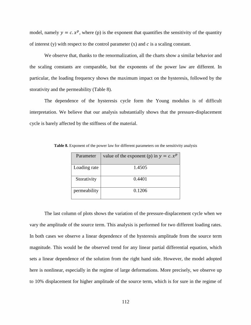
112

model, namely 𝑦𝑦 = 𝑐𝑐. 𝑑𝑑𝑝𝑝, where (p) is the exponent that quantifies the sensitivity of the quantity

of interest (y) with respect to the control parameter (x) and 𝑐𝑐 is a scaling constant.

We observe that, thanks to the renormalization, all the charts show a similar behavior and

the scaling constants are comparable, but the exponents of the power law are different. In

particular, the loading frequency shows the maximum impact on the hysteresis, followed by the

storativity and the permeability (Table 8).

The dependence of the hysteresis cycle form the Young modulus is of difficult

interpretation. We believe that our analysis substantially shows that the pressure-displacement

cycle is barely affected by the stiffness of the material.

Table 8. Exponent of the power law for different parameters on the sensitivity analysis

Parameter value of the exponent (p) in 𝑦𝑦 = 𝑐𝑐. 𝑑𝑑𝑝𝑝

Loading rate 1.4505

Storativity 0.4401

permeability 0.1206

The last column of plots shows the variation of the pressure-displacement cycle when we

vary the amplitude of the source term. This analysis is performed for two different loading rates.

In both cases we observe a linear dependence of the hysteresis amplitude from the source term

magnitude. This would be the observed trend for any linear partial differential equation, which

sets a linear dependence of the solution from the right hand side. However, the model adopted

here is nonlinear, especially in the regime of large deformations. More precisely, we observe up

to 10% displacement for higher amplitude of the source term, which is for sure in the regime of

113

large deformations and therefore we need large deformation formulation to handle this problem.

Indeed, the results confirm that this is when we have significant poroelastic coupling effect and

hysteresis loop. However, we observe that by increasing the loading amplitude the hysteresis

indicator shows linear increase with respect to the loading amplitude which says that the

response of the model to variation of the load is still linear.

114

5.0 CONCLUSION

In the context of hemodynamics, we have developed a computational model for the

interaction between pulsatile fluid flow in a channel, confined with a thick poroelastic wall. In

order to approximate this problem, we have proposed and analyzed a partitioned, loosely coupled

finite element solver based on weak enforcement of interface conditions using Nitsche’s method

that allows us to independently solve the equations at each time step. Namely, structure

mechanics, the intramural filtration and the fluid flow problem are solved separately at each time

step. In this way, we uncouple the original problem into the parts defined on separate sub-

regions, which leads to a more efficient calculation of the numerical solution. This method can

accommodate a mixed formulation for the Darcy’s equations and it guarantees stability as well,

provided that several penalty and stabilization parameters are appropriately selected. To improve

the accuracy of the scheme, we have also considered its application as a preconditioner for the

fully coupled (monolithic) FSI problem formulation, with very encouraging results both for

performance and accuracy of the method. The theoretical results have been complemented by

numerical simulations. We have tested our algorithm on 2D and 3D idealized geometries to

simulate the propagation of the pressure waves and the related wall deformation. Also, our

computational method allowed us get an accurate representation of the intramural flow within

the wall.

115

Also, we have performed a sensitivity analysis of the effects of poroelastic parameters on

FSI results. More precisely, by means of a collection of numerical experiments, we qualitatively

analyze how the poroelastic phenomena affect the propagation of pressure waves and the wall

displacement. We conclude that increasing the hydraulic permeability (leaky domain) decreases

the amplitude of pressure wave, which means that we have more dissipation.

In order to enhance our understanding of the underlying phenomena of poroelasticity, we

have analyzed the role of intramural fluid flow in the apparent viscoelastic behavior of the

poroelastic wall. To this aim, we have studied the energy exchange in the interaction between

the blood flow and the arterial wall, to investigate the distribution and dissipation of the energy

delivered to the artery during one heart cycle. We have compared the energy distribution when

the wall is modeled using different constitutive models: namely elastic, viscoelastic and

poroelastic. Although this analysis has informed us about qualitative energy exchange due to

conductivity of the pores and corresponding filtration velocity, we haven’t observed any

hysteresis loop for the poroelastic model. Therefore, based on the hypothesis that large

deformations and nonlinear elasticity may trigger the poroelastic effects, we have moved to finite

elasticity formulation of the poroelastic media in a FSI framework.

We have investigated numerically the effects of poroelasticity parameters, as well as

loading rate and loading magnitude, on the energy dissipation. Namely, we distinguish a fast

loading rate, a high storativity and a high permeability case in the Darcy equations, and the

obtained hysteresis loops are compared for different values of each model parameter. By

employing finite elasticity in our FPSI solver, the results show that the energy loss differs

substantially between poroelastic model and elastic wall models, and confirmed that accurate

116

representation of the structure model as a poroelastic medium is essential for low loading

frequencies, and high hydraulic conductivity and storativity.

Both poroelasticity and viscoelasticity are coupled solid-fluid problems but in different

ways. Perhaps the most interesting feature of the model studied in this work is its capability of

explicitly capturing these two distinct phenomena. Namely, one is the influence of fluid viscosity

on the vessel wall dynamics (poroelasticity), and a separate one is the vessel wall viscoelastic

mechanical properties that is modeled by utilizing a linearly viscoelastic model based on Kelvin-

Voigt viscoelasticity. It is shown that the mechanism of the energy dissipation of the poroelastic

material is different from that of a conventional solid material because of the interaction between

the fluid and solid phase. In the poroelastic material, the energy dissipation and related hysteresis

loop is not primarily because of effects within the material of the skeleton itself. It is because the

skeleton is permeated with fluid. Therefore, we conclude that the effect of the transmural flow in

the total structure stress should be accounted depends on poroelastic parameters value. In

summary, the results in this thesis highlight the importance of including both poroelasticity and

viscoelasticity in modeling fluid-structure interaction.

All the previous results illustrate the role of poroelasticity on the mechanics of soft

tissues in general. For the specific case of cardiovascular applications, some partially conclusive

results are available in Chapter 3. There, we have performed a test case that resembles a medium

size artery, see in particular Section 3.4.2 “Benchmark 2: FSI analysis under physiological

condition”. This test case highlights some characteristic features on the poro-visco-elastic

behavior of an artery, which are outlined below:

• The dissipative effect of intramural flow on the mechanical energy of the artery, is

relevant for high hydraulic conductivities of the arterial wall. These values are

117

significantly larger than the physiological permeability of healthy arteries (see

Table 5). Indeed, in Section 3.4.2, benchmark problem 2, we barely see any effect

for poroelasticity when comparing it to the elastic one for the physiological range

of permeability parameter. For larger values of permeability, our results confirm

that the poroelastic model appreciably changes the displacement and wave

propagation speed in structure as well as the energy distribution.

• In the physiological range of material parameters, the viscous dissipation in the

blood flow is the dominant dissipative term during a heartbeat. Only in the range

of high vascular permeability and in the late diastole phase, intramural filtration

dissipates comparable amount of energy (see Figure 17 of Chapter 3). For small

permeability values, we barely notice any contribution related to intramural

filtration. We also observe that the energy dissipated in the wall is a small fraction

of that dissipated by the fluid.

• If a viscoelastic behavior is accounted for, non-negligible energy losses can be

observed even in the case of healthy tissue (see Figure 17).

• Viscoelasticity is responsible for establishing a hysteresis loop in the pressure vs

displacement plots. In contrast, poroelasticity does not generate any hysteresis,

under physiological conditions (see Figure 19).

• The results of Chapter 4 (more precisely Figures 29-35) also suggest that high

deformation rates in the solid matrix trigger effects of hysteresis in the poroelastic

material. However, to observe these effects, the deformations rates that we use are

remarkably higher than the physiological ones.

118

These conclusions will be further strengthened when a few limitations of this work will

be overcome:

• The computational results are affected by significant uncertainty on the

physiological parameters characterizing the poro-visco-elastic behavior of an

artery. To our best knowledge, the parameters that describe a healthy artery are

collected in Table 5. Better experiments or more advanced modeling approaches

based on mathematical homogenization might in future fill this knowledge gap.

• We did not explore the variations of the geometric configuration of the artery, but

we are aware that the conclusions of this study may no longer apply to small

arteries, such as the cerebral arteries, for example.

• At the level of numerical methods, more accurate discretization schemes may be

adopted, in order to improve the mass and energy conservation properties of the

simulator.

For future work, the main focus will be to minimize the computational cost due to the

iterations between the fluid and solid sub problems, especially in the nonlinear solver.

Decreasing computational cost, makes us able to solve for more complicated geometries which is

particularly important for the biomedical applications of this work, namely for the interaction

between the blood flow and the arterial wall, to reach the goal of simulating realistic vascular

districts. Another interesting application of this work will be to simulate LDL transport or drug

delivery through the arterial walls, with pulsatile blood flow. In this case, a mass transfer model,

coupled to the FPSI problem shall be implemented. In [101, 102] a mathematical model has been

developed to capture the interplay between blood perfusion, fluid exchange with the interstitial

volume, and mass transport in the capillary bed, through the capillary walls and into the

119

surrounding tissue. Our model can be combined with [101] to provide a poroelastic description

of the interstitial tissue, in order to capture the interplay of mechanical deformations and

transport phenomena.

120

BIBLIOGRAPHY

1. Chapelle, D., et al., A poroelastic model valid in large strains with applications to perfusion in cardiac modeling. Computational Mechanics, 2009. 46(1): p. 91-101.

2. Calo, V.M., et al., Multiphysics model for blood flow and drug transport with application to patient-specific coronary artery flow. Computational Mechanics, 2008. 43(1): p. 161-177.

3. Feenstra, P.H. and C.A. Taylor, Drug transport in artery walls: A sequential porohyperelastic-transport approach. Computer Methods in Biomechanics and Biomedical Engineering, 2009. 12(3): p. 263-276.

4. Badia, S., A. Quaini, and A. Quarteroni, Coupling Biot and Navier-Stokes equations for modelling fluid-poroelastic media interaction. Journal of Computational Physics, 2009. 228(21): p. 7986-8014.

5. Koshiba, N., et al., Multiphysics simulation of blood flow and LDL transport in a porohyperelastic arterial wall model. J Biomech Eng, 2007. 129(3): p. 374-85.

6. McCutchen, C.W., Cartilage is poroelastic, not viscoelastic (including and exact theorem about strain energy and viscous loss, and an order of magnitude relation for equilibration time). Journal of Biomechanics, 1982. 15(4): p. 325-327.

7. Yang, Z. and P. Smolinski, Dynamic finite element modeling of poroviscoelastic soft tissue. Computer Methods in Biomechanics and Biomedical Engineering, 2006. 9(1): p. 7-16.

8. Bukac, M., et al., Effects of Poroelasticity on Fluid-Structure Interaction in Arteries: a Computational Sensitivity Study, in Modeling the Heart and the Circulatory System. 2015, Springer. p. 197-220.

9. Prosi, M., et al., Mathematical and numerical models for transfer of low-density lipoproteins through the arterial walls: a new methodology for the model set up with applications to the study of disturbed lumenal flow. J Biomech, 2005. 38(4): p. 903-17.

10. Chepelenko, G.V., Atherosclerosis regulation via media lipid-driven VSMC cholesterol efflux switch. Medical Hypotheses, 2015. 84(2): p. 141-144.

121

11. Smith, E., Transport, interactions and retention of plasma proteins in the intima: the barrier function of the internal elastic lamina. European heart journal, 1990. 11(suppl E): p. 72-81.

12. Smith, E. and R. Slater. In Atherogenesis: Initiating Factors. in Ciba Foundation Symposia, New Series. 1973.

13. Bertolotti, C. and V. Deplano, Three-dimensional numerical simulations of flow through a stenosed coronary bypass. J Biomech, 2000. 33(8): p. 1011-22.

14. Bazilevs, Y., et al., Isogeometric fluid-structure interaction analysis with applications to arterial blood flow. Computational Mechanics, 2006. 38(4-5): p. 310-322.

15. Nichols, W., M. O'Rourke, and C. Vlachopoulos, McDonald's Blood Flow in Arteries, Sixth Edition: Theoretical, Experimental and Clinical Principles. 2011: Taylor & Francis.

16. Armentano, R.L., et al., Arterial wall mechanics in conscious dogs. Assessment of viscous, inertial, and elastic moduli to characterize aortic wall behavior. Circ Res, 1995. 76(3): p. 468-78.

17. Čanić, S., et al., Modeling viscoelastic behavior of arterial walls and their interaction with pulsatile blood flow. SIAM Journal on Applied Mathematics, 2006. 67(1): p. 164-193.

18. Fung, Y., et al., Biomechanics, its foundations and objectives. 1972: Prentice-Hall.

19. Holzapfel, G.A., T.C. Gasser, and M. Stadler, A structural model for the viscoelastic behavior of arterial walls: Continuum formulation and finite element analysis. European Journal of Mechanics, A/Solids, 2002. 21(3): p. 441-463.

20. Causin, P., J.F. Gerbeau, and F. Nobile, Added-mass effect in the design of partitioned algorithms for fluid–structure problems. Computer Methods in Applied Mechanics and Engineering, 2005. 194(42–44): p. 4506-4527.

21. Kennedy, J.M. and T.B. Belytschko, Theory and application of a finite element method for arbitrary Lagrangian-Eulerian fluids and structures. Nuclear Engineering and Design, 1982. 68(2): p. 129-146.

22. MIKELIĆ, A. and M.F. WHEELER, ON THE INTERFACE LAW BETWEEN A DEFORMABLE POROUS MEDIUM CONTAINING A VISCOUS FLUID AND AN ELASTIC BODY. Mathematical Models and Methods in Applied Sciences, 2012. 22(11): p. 1250031.

23. Ganis, B., et al., Modeling fractures in a poro-elastic medium. Oil & Gas Science and Technology–Revue d’IFP Energies nouvelles, 2014. 69(4): p. 515-528.

122

24. Girault, V., et al., A lubrication fracture model in a poro-elastic medium. Mathematical Models and Methods in Applied Sciences, 2014: p. 1-59.

25. Badia, S., A. Quaini, and A. Quarteroni, Coupling Biot and Navier–Stokes equations for modelling fluid–poroelastic media interaction. Journal of Computational Physics, 2009. 228(21): p. 7986-8014.

26. Zakerzadeh, R., et al. Computational models for fluid-structure interaction with a poroelastic structure. in APS Division of Fluid Dynamics Meeting Abstracts. 2013.

27. Bukač, M., et al., Partitioning strategies for the interaction of a fluid with a poroelastic material based on a Nitsche’s coupling approach. Computer Methods in Applied Mechanics and Engineering, 2015. 292: p. 138-170.

28. Zakerzadeh, R. and P. Zimino. Fluid-structure interaction in arteries with a poroelastic wall model. in Biomedical Engineering (ICBME), 2014 21th Iranian Conference on. 2014. IEEE.

29. Zakerzadeh, R. and P. Zunino, Fluid-Structure Interaction in Arteries with a Poroelastic Wall Model. 21st Iranian Conference of Biomedical Engineering (ICBME) IEEE,: p. 35 - 39.

30. Zakerzadeh, R., M. Bukac, and P. Zunino, Computational analysis of energy distribution of coupled blood flow and arterial deformation. International Journal of Advances in Engineering Sciences and Applied Mathematics, 2015: p. 1-16.

31. Zakerzadeh, R. and P. Zunino, Fluid-Structure interaction modeling in deformable porous arteries. Bulletin of the American Physical Society, 2015. 60.

32. Zakerzadeh, R. and P. Zunino, Numerical modeling of fluid-porous structure interaction in arteries. 2016.

33. Tully, B. and Y. Ventikos, Coupling poroelasticity and cfd for cerebrospinal fluid hydrodynamics. IEEE Transactions on Biomedical Engineering, 2009. 56(6): p. 1644-1651.

34. Ma, X., G.C. Lee, and S.G. Wu, Numerical Simulation for the Propagation of Nonlinear Pulsatile Waves in Arteries. Journal of Biomechanical Engineering, 1992. 114(4): p. 490-496.

35. Bukač, M., et al., Partitioning strategies for the interaction of a fluid with a poroelastic material based on a Nitsche’s coupling approach. Computer Methods in Applied Mechanics and Engineering, 2014.

36. Hansbo, P., Nitsche's method for interface problems in computa-tional mechanics. GAMM-Mitteilungen, 2005. 28(2): p. 183-206.

123

37. Burman, E. and M.A. Fernández, Stabilization of explicit coupling in fluid-structure interaction involving fluid incompressibility. Computer Methods in Applied Mechanics and Engineering, 2009. 198(5-8): p. 766-784.

38. Burman, E. and M.A. Fernández, Explicit strategies for incompressible fluid-structure interaction problems: Nitsche type mortaring versus Robin–Robin coupling. International Journal for Numerical Methods in Engineering, 2014. 97(10): p. 739-758.

39. Ambartsumyan, I., et al., Simulation of Flow in Fractured Poroelastic Media: A Comparison of Different Discretization Approaches, in Finite Difference Methods,Theory and Applications: 6th International Conference, FDM 2014, Lozenetz, Bulgaria, June 18-23, 2014, Revised Selected Papers, I. Dimov, I. Faragó, and L. Vulkov, Editors. 2015, Springer International Publishing: Cham. p. 3-14.

40. Bukac, M., Yotov, I., Zakerzadeh, R., and Zunino P., Effect of poroelasticity on fluid-structure interaction in arteries: a computational sensitivity study. Modeling the heart and the circulatory system, 2014. vol 13 (MS&A, Springer Italia).

41. Hecht, F., New development in freefem+. Journal of Numerical Mathematics, 2012. 20(3-4): p. 251-265.

42. Bukač, M., et al., Fluid-structure interaction in blood flow capturing non-zero longitudinal structure displacement. Journal of Computational Physics, 2013. 235: p. 515-541.

43. Quarteroni, A. and A. Valli, Numerical approximation of partial differential equations. Vol. 23. 2008: Springer Science & Business Media.

44. Brezzi, F. and J. Pitkäranta, On the Stabilization of Finite Element Approximations of the Stokes Equations, in Efficient Solutions of Elliptic Systems: Proceedings of a GAMM-Seminar Kiel, January 27 to 29, 1984, W. Hackbusch, Editor. 1984, Vieweg+Teubner Verlag: Wiesbaden. p. 11-19.

45. Nobile, F., M. Pozzoli, and C. Vergara, Time accurate partitioned algorithms for the solution of fluid–structure interaction problems in haemodynamics. Computers & Fluids, 2013. 86(0): p. 470-482.

46. Caro, C.G., et al., The mechanics of the circulation, second edition. The Mechanics of the Circulation, Second Edition. 2011. 1-524.

47. Barbenel, J.C., The Arterial Wall, in Arteries and Arterial Blood Flow, C.M. Rodkiewicz, Editor. 1983, Springer Vienna. p. 129-177.

48. Humphrey, J.D. and S.L. Delange, An Introduction to Biomechanics: Solids and Fluids, Analysis and Design. 2004: Springer.

49. Cowin, S.C. and J.D. Humphrey, Cardiovascular soft tissue mechanics. 2001: Springer.

124

50. Cowin, S.C. and S.B. Doty, Tissue mechanics. Tissue Mechanics. 2007. 1-682.

51. Formaggia, L., et al., On the coupling of 3D and 1D Navier-Stokes equations for flow problems in compliant vessels. Computer Methods in Applied Mechanics and Engineering, 2001. 191(6-7): p. 561-582.

52. Gerbeau, J.-F., M. Vidrascu, and P. Frey, Fluid–structure interaction in blood flows on geometries based on medical imaging. Computers & Structures, 2005. 83(2–3): p. 155-165.

53. Nobile, F., Numerical approximation of fluid-structure interaction problems with application to haemodynamics. 2001, EPFL.

54. Skalak, R., et al., The Energy Distribution in the Pulmonary Circulation, II: Experiments. Physics in Medicine and Biology, 1966. 11(3): p. 437.

55. Skalak, R., et al., The Energy Distribution in the Pulmonary Circulation, I: Theory. Physics in Medicine and Biology, 1966. 11(2): p. 287.

56. Bertram, C.D., Energy dissipation and pulse wave attenuation in the canine carotid artery. Journal of Biomechanics, 1980. 13(12): p. 1061-1073.

57. Tsaturyan, A.K., et al., Extracellular fluid filtration as the reason for the viscoelastic behaviour of the passive myocardium. Journal of Biomechanics, 1984. 17(10): p. 749-755.

58. Huyghe, J.M., Non-linear finite element models of the beating left ventricle and the intramyocardial coronary circulation. Ph.D. thesis, 1986.

59. Yang, M. and L.A. Taber, The possible role of poroelasticity in the apparent viscoelastic behavior of passive cardiac muscle. J Biomech, 1991. 24(7): p. 587-97.

60. Armentano, R., et al., Effects of hypertension on viscoelasticity of carotid and femoral arteries in humans. Hypertension, 1995. 26(1): p. 48-54.

61. London, G.M. and B. Pannier, Arterial functions: how to interpret the complex physiology. Nephrology dialysis transplantation, 2010. 25(12): p. 3815-3823.

62. Canic, S., et al., Blood flow in compliant arteries: an effective viscoelastic reduced model, numerics, and experimental validation. Ann Biomed Eng, 2006. 34(4): p. 575-92.

63. Bukac, M. and S. Canic, Longitudinal displacement in viscoelastic arteries: a novel fluid-structure interaction computational model, and experimental validation. Math Biosci Eng, 2013. 10(2): p. 295-318.

64. Badia, S., A. Quaini, and A. Quarteroni, Splitting methods based on algebraic factorization for fluid-structure interaction. SIAM Journal on Scientific Computing, 2007. 30(4): p. 1778-1805.

125

65. Warriner, R.K., K.W. Johnston, and R.S.C. Cobbold, A viscoelastic model of arterial wall motion in pulsatile flow: Implications for Doppler ultrasound clutter assessment. Physiological Measurement, 2008. 29(2): p. 157-179.

66. Badia, S., A. Quaini, and A. Quarteroni, Splitting methods based on algebraic factorization for fluid-structure interaction. SIAM Journal on Scientific Computing, 2008. 30(4): p. 1778-1805.

67. Grandmont, C., M. Lukáčová-Medvid’ová, and Š. Nečasová, Mathematical and Numerical Analysis of Some FSI Problems, in Fluid-Structure Interaction and Biomedical Applications, T. Bodnár, G.P. Galdi, and Š. Nečasová, Editors. 2014, Springer Basel. p. 1-77.

68. Muha, B. and S. Čanić, Existence of a solution to a fluid–multi-layered-structure interaction problem. Journal of Differential Equations, 2014. 256(2): p. 658-706.

69. Bukac, M., Yotov, I., Zakerzadeh, R., and Zunino P. Partitioning strategies for the interaction of a fluid with a poroelastic material based on a Nitsche's coupling approach. ArXiv e-prints, 2014. 1403, 5707.

70. Brooks, A.N. and T.J. Hughes, Streamline upwind/Petrov-Galerkin formulations for convection dominated flows with particular emphasis on the incompressible Navier-Stokes equations. Computer methods in applied mechanics and engineering, 1982. 32(1): p. 199-259.

71. Hasegawa, H. and H. Kanai, Measurement of elastic moduli of the arterial wall at multiple frequencies by remote actuation for assessment of viscoelasticity. Japanese journal of applied physics, 2004. 43(5S): p. 3197.

72. Bukač, M., et al., A modular, operator-splitting scheme for fluid-structure interaction problems with thick structures. International Journal for Numerical Methods in Fluids, 2014. 74(8): p. 577-604.

73. Quaini, A., Algorithms for fluid-structure interaction problems arising in hemodynamics. 2009.

74. Bukac, M., A Fluid-structure Interaction Model Capturing Longitudinal Displacement in Arteries: Modeling, Computational Method, and Comparison with Experimental Data. 2012, University of Houston.

75. Craiem, D., et al., Cardiovascular engineering: modelization of ventricular-arterial interaction in systemic and pulmonary circulation. Latin American applied research, 2005. 35(2): p. 111-114.

76. Polzer, S., et al., Impact of poroelasticity of intraluminal thrombus on wall stress of abdominal aortic aneurysms. BioMedical Engineering OnLine, 2012. 11: p. 62-62.

126

77. Govindaraju, K., et al., Effect of porous media of the stenosed artery wall to the coronary physiological diagnostic parameter: a computational fluid dynamic analysis. Atherosclerosis, 2014. 233(2): p. 630-5.

78. Page, R.C. and H.E. Schroeder, Pathogenesis of inflammatory periodontal disease. A summary of current work. Lab Invest, 1976. 34(3): p. 235-49.

79. Ayyalasomayajula, A., J.P. Vande Geest, and B.R. Simon, Porohyperelastic finite element modeling of abdominal aortic aneurysms. J Biomech Eng, 2010. 132(10): p. 104502.

80. Dabagh, M., et al., Distribution of shear stress over smooth muscle cells in deformable arterial wall. Med Biol Eng Comput, 2008. 46(7): p. 649-57.

81. Prosi, M., et al., Mathematical and numerical models for transfer of low-density lipoproteins through the arterial walls: a new methodology for the model set up with applications to the study of disturbed lumenal flow. Journal of Biomechanics, 2005. 38(4): p. 903-917.

82. Balzani, D., et al., Numerical modeling of fluid–structure interaction in arteries with anisotropic polyconvex hyperelastic and anisotropic viscoelastic material models at finite strains. International journal for numerical methods in biomedical engineering, 2015.

83. Tricerri, P., et al., Fluid-structure interaction simulations of cerebral arteries modeled by isotropic and anisotropic constitutive laws. Computational Mechanics, 2015. 55(3): p. 479-498.

84. Quaini, A. and A. Quarteroni, A semi-implicit approach for fluid-structure interaction based on an algebraic fractional step method. Mathematical Models and Methods in Applied Sciences, 2007. 17(6): p. 957-983.

85. Taber, L.A. and A.M. Puleo, Poroelastic plate and shell theories, in Mechanics of Poroelastic Media. 1996, Springer. p. 323-337.

86. Costi, J.J., et al., Frequency-dependent behavior of the intervertebral disc in response to each of six degree of freedom dynamic loading: solid phase and fluid phase contributions. Spine, 2008. 33(16): p. 1731.

87. Le Tallec, P. and J. Mouro, Fluid structure interaction with large structural displacements. Computer Methods in Applied Mechanics and Engineering, 2001. 190(24): p. 3039-3067.

88. Discacciati, M. and A. Quarteroni, Navier-Stokes/Darcy coupling: modeling, analysis, and numerical approximation. Revista Matemática Complutense, 2009. 22(2): p. 315-426.

127

89. Uzuoka, R. and R.I. Borja, Dynamics of unsaturated poroelastic solids at finite strain. International Journal for Numerical and Analytical Methods in Geomechanics, 2012. 36(13): p. 1535-1573.

90. Quarteroni, A., R. Sacco, and F. Saleri, Numerical mathematics. Vol. 37. 2010: Springer Science & Business Media.

91. Razzaq, M., et al., Numerical Simulation and Benchmarking of Fluid Structure Interaction with Application to Hemodynamics. 2009: Techn. Univ., Fak. für Mathematik.

92. Jendoubi, A., J. Deteix, and A. Fortin, A simple mesh-update procedure for fluid–structure interaction problems. Computers & Structures, 2016. 169: p. 13-23.

93. Finite Element Methods, in Robust Numerical Methods for Singularly Perturbed Differential Equations: Convection-Diffusion-Reaction and Flow Problems. 2008, Springer Berlin Heidelberg: Berlin, Heidelberg. p. 277-425.

94. Ijiri, T., et al., A Kinematic Approach for Efficient and Robust Simulation of the Cardiac Beating Motion. PLoS ONE, 2012. 7(5): p. e36706.

95. Ravi, S. and E.L. Chaikof, Biomaterials for vascular tissue engineering. Regenerative medicine, 2010. 5(1): p. 107.

96. Bjork, J.W. and R.T. Tranquillo, Transmural flow bioreactor for vascular tissue engineering. Biotechnology and bioengineering, 2009. 104(6): p. 1197-1206.

97. Biot, M.A., Theory of propagation of elastic waves in a fluid‐saturated porous solid. I. Low‐frequency range. The Journal of the acoustical Society of america, 1956. 28(2): p. 168-178.

98. Ren, H., G. Goloshubin, and F.J. Hilterman, Poroelastic analysis of permeability effects in thinly layered porous media. Geophysics, 2009. 74(6): p. N49-N54.

99. Cederbaum, G., L. Li, and K. Schulgasser, Poroelastic structures. 2000: Elsevier.

100. Yeh, F.-H. and H.-S. Tsay, Dynamic behavior of a poroelastic slab subjected to uniformly distributed impulsive loading. Computers & Structures, 1998. 67(4): p. 267-277.

101. Nabil, M., P. Decuzzi, and P. Zunino, Modelling mass and heat transfer in nano-based cancer hyperthermia. Royal Society Open Science, 2015. 2(10).

102. Nabil, M., P. Zunino, and L. Cattaneo, A Computational Study of Microscale Flow and Mass Transport in Vasculatized Tumors. 21st Iranian Conference of Biomedical Engineering (ICBME) Pages 23-28, IEEE,, 2015.

d-scholarship.pitt.edud-scholarship.pitt.edu/28595/1/zakerzadeh_etdpitt2016.pdf · in this work, we...

Documents