d1.1 roadmap for regional end-users on how to collect

S2Biom Project Grant Agreement n°608622

D1.1

Roadmap for regional end-users on how to collect, process, store and maintain biomass supply data

Version: 1.1

19.04.2017

Delivery of sustainable supply of non-food biomass to support a “resource-efficient” Bioeconomy in Europe

D1.1

1

About S2Biom project

The S2Biom project - Delivery of sustainable supply of non-food biomass to support a “resource-efficient” Bioeconomy in Europe - supports the sustainable delivery of non-food biomass feedstock at local, regional and pan European level through developing strategies, and roadmaps that will be informed by a “computerized and easy to use” toolset (and respective databases) with updated harmonized datasets at local, regional, national and pan European level for EU28, Western Balkans, Moldova, Turkey and Ukraine. Further information about the project and the partners involved are available under www.s2biom.eu.

Project coordinator

Scientific coordinator

Project partners

D1.1

2

About this document

It has been prepared by:

Due date of deliverable: PM 30 Actual submission date: 19. April 2017 Start date of project: 2013-01-09 Duration: 39 months Work package 1 Task Sustainable biomass cost-supply Lead contractor for this deliverable

ALU-FR

Editor Matthias Dees Authors Matthias Dees, Pawan Datta (ALU-FR);

Joanne Fitzgerald, Hans Verkerk, Marcus Lindner (EFI); Berien Elbersen, Raymond Schrijver, Igor Staritsky & Kees van Diepen (DLO [Alterra]); Jacqueline Ramirez-Almeyda, Andrea Monti (UniBo) Martijn Vis (BTG) Branko Glavonjic (University of Belgrade)

Quality reviewer Calliope Panoutsou (UC)

Dissemination Level

PU Public X PP Restricted to other programme participants (including the Commission Services) RE Restricted to a group specified by the consortium (including the Commission Services): CO Confidential, only for members of the consortium (including the Commission Services)

Version Date Reason for modification

1.0 23/01/2017 First version.

1.1 19/04/2017 Minor editorial corrections concerning orthography, the statements referring to the 7th Framework Programme and the authorship responsibility.

This project entitled S2BIOM (Delivery of sustainable supply of non-food biomass to support a “resource-efficient” Bioeconomy in Europe) is co-funded by the European Union within the 7th Framework Programme. Grant Agreement n°608622.

The sole responsibility of this publication lies with the author. The European Union is not responsible for any use that may be made of the information contained therein.

Editor contact details: Ass. Prof. Dr. Matthias Dees Chair of Remote Sensing and Landscape Information Systems Institute of Forest Sciences University of Freiburg Mailing address: D-79085 Freiburg, Germany Delivery address: Tennenbacherstr. 4, D-79106 Freiburg, Germany Tel.: +49-761-203-3697 // +49-7666-912506 [email protected]

D1.1

3

Recommended citation: Dees, M., Elbersen, B., Fitzgerald, J., Vis, M., Ramirez-Almeyda, J., Glavonjic, B., Staritsky, I., Verkerk, H., Monti, A., Datta, P., Schrijver, R., Lindner, M. & Diepen, K. (2017): Roadmap for regional end-users on how to collect, process, store and maintain biomass supply data. Project Report. S2BIOM – a project funded under the European Union 7th Framework Programme for Research. Grant Agreement n°608622. Chair of Remote Sensing and Landscape Information Systems, Institute of Forest Sciences, University of Freiburg, Germany. 80 p.

D1.1

4

Table of contents

Table of contents ...................................................................................................... 4

List of Figures ........................................................................................................... 6

List of Tables ............................................................................................................ 6

1 Introduction ....................................................................................................... 8

2 Biomass assessment ........................................................................................ 9

2.1 Introduction ................................................................................................. 9

2.2 Types of potentials and approach for estimating potentials ...................... 10

2.2.1 Overall approach for estimating the potentials ...................................................... 12

3 Determination of the sustainable technical potential ................................... 13

3.1 Stemwood and primary forestry residues ................................................. 13

3.1.1 Potential categories and potential types ............................................................... 13

3.1.2 Methods for assessing potentials .......................................................................... 13

3.1.3 Data needs, main data sources, database and modelling requirements .............. 16

3.2 Secondary residues from wood industry .................................................. 18


3.2.2 Methods ................................................................................................................ 18

3.2.2.1 Introduction ........................................................................................................ 18

3.2.2.2 Saw mill residues ............................................................................................... 19

3.2.2.3 Secondary residues from semi-finished wood based panels ............................ 24

3.2.2.4 Secondary residues from further processing ..................................................... 25

3.2.2.5 Residues from pulp and paper .......................................................................... 27

3.2.2.6 Spatial disaggregation ....................................................................................... 28

3.2.2.7 Methods used to estimate future potentials ....................................................... 29

3.3 Primary residues from agriculture ............................................................. 30



3.3.2.1 Straw & stubbles from arable crops ................................................................... 30

3.3.2.2 Prunings from permanent crops ........................................................................ 36

3.3.3 Data needs and main data sources ...................................................................... 45

3.4 Biomass cropping potentials ..................................................................... 49



3.4.3 Data needs, main data sources and modelling requirements ............................... 60

D1.1

5

3.5 Secondary residues from agriculture ........................................................ 62

3.6 Biomass from other land categories then forest and agricultural lands .... 65



3.7 Biomass from waste ................................................................................. 66


3.7.1.1 Biowaste 66

3.7.1.2 Post-consumer wood ......................................................................................... 67


3.7.2.1 Biowaste 67


3.7.3 Data needs, main data sources and modelling requirements ............................... 71

3.7.3.1 Biowaste 71


4 Main recommendation and conclusions ....................................................... 73

5 References ....................................................................................................... 74

D1.1

6

List of Figures

Figure 1 Model of cascading use of woody biomass (Steierer 2010) 22 Figure 2 Type of lands considered available for energy crop cultivation according to Allen

et al. (2014) 53 Figure 3 Direct and indirect land use effects (source: EEA, 2013 made by Uwe Fritsche,

IINAS) 57

List of Tables

Table 1 Types of biomass potentials according to BEE (Torén, J. et al., 2011) 10 Table 2 Overview of combinations of approaches and methodologies for biomass energy

assessment to investigate different types of biomass potentials (copied from BEE report ‘Executive summary, evaluation and recommendations’ Torén, J. et al., 2011) 11

Table 3 Subcategories of first level category 1 “Forestry” 13 Table 4 Example data sources for use in EFISCEN 17 Table 5 Subcategories of second level category 41 “Secondary residues from wood

industries” 18 Table 6 Sawmill residue to product ratios per country, Conifers 20 Table 7 Sawmill residue to product ratios per country, Nonconifers 21 Table 8 Deduction factor to account for residues that are utilised in paper and board

production, 23 Table 9 Overview and definition of semi-finished wood based panels 24 Table 10 Factors used to determined secondary residues from semi-finished wood based

panels 25 Table 11 Business sub-sectors from structural business statistics utilised to determine

the number of employees for the estimation of the residues from further processing 26

Table 12 Factors used to determined secondary residues from further processing 26 Table 13 Wood consumption [m³] per employee in Western Balkan countries 27 Table 14 Conversion factor round wood input / ton pulp 27 Table 15 Share of round wood in the pulp and paper industry 28 Table 16 Spatial disaggregation approach by sector 29 Table 17 Subcategories primary agricultural residues 30 Table 18 Residue-to-yield factors used in different studies. (’Yield’ refers to yield of main

crop which is the grain). 31 Table 19 Straw-to-crop yield ratios as determined by the correlations from Scarlat et al.

(2010) elaborated in ECOFYS study (Spöttle, et. al. 2013). 32 Table 20 Sustainable removal rates considered by Scarlat et al. (2010) 34 Table 21 Sustainable removal rates identified by ECOFYS (Spöttle, et. al. 2013) 34 Table 22 Permanent crop pruning practices and average pruning yield (Ton/Ha/Y fm) 38 Table 23 National average maximum Residue to Surface Ratio (RSR) per country 40 Table 24 Current pruning management practices in Europe. The practice ‘Shredded and

left/incorporated to soil’ refer to the level of prunings that are kept in the field for maintenance of SOC and nutrients in the soil. 43

D1.1

7

Table 25 Overview of unused pruning shares (=% already going to energy and/or not removed or used for soil improvement) in 2012 which are the results of an analysis of the data in Table 24 44

Table 26 Overview of data sources providing information on area and yields to be used as input for calculation of straw potentials 45

Table 27 FSS permanent crop categories included in FSS and surfaces (ha) in 2010 47 Table 28 Key models for land availability and cropped biomass potential assessment 55 Table 29 Environmental pressures and their link to biodiversity (source: EEA, 2007) 59 Table 30 Overview of main EU and international data sources on land use 60 Table 31 Overview of selection of most common secondary agricultural residues in

Europe 63 Table 32 Example of information and possible data sources to calculate the road side

verge grassland potential 66

D1.1

8

1 Introduction

This report intends to provide support to institutional, private sector and scientist that intend to establish a potential supply data base for lignocellulose non-food biomass from regional (subnational, cross national border regional) to national level and complements the other documents and deliverables of Work Package 5 (D1.2. to D1.8) that have the focus on the establishment of a data base by the project S2BIOM at national to European level with a spatial resolution of NUTS3, the third level of EU’s statistical units

Recommendations on the use of data sources, methods and the establishment and maintenance of biomass databases are provided. This includes guidelines to assess the biomass potential for the main biomass categories for both agriculture, forestry and waste sectors in order to propose a standardized approach to be repeated by practitioners working in the field of biomass utilisation for non-food purposes.

The report covers all major origins and categories and utilises the method reports and guidelines of the projects BEE, EUROPRUNING, EUWOOD, BIOMASS POLICIES, which have been the background projects for S2Biom, and makes use of the methodology developed and applied to set up the S2BIOM database.

The guidelines presented here can be used both to set up regional level data sets but as well to provide more accurate estimates using national level data sources for future updates of the S2BIOM database.

Where feasible approaches proposed in this report to increase the accuracy of the estimates at regional level by utilising national level data sources have already been applied when setting up the S2BIOM database.

When a regional biomass database is set up, definitions of the scope are required. The spatial scale, the spatial extend and the attributes per spatial unit needs to be specified. A data base addressing both the spatial units, the temporal dimension, the categories and the potential levels to be covered needs to be set up and may follow the S2BIOM data base design that is described in the report D1.5 and that is providing a clear structure supporting adjustments to regional needs or future adjustments.

The focus of this report is on the assessment methods for estimating ligno-cellulosic biomass potentials. The report follows essentially the description of the approach used to set up the S2BIOM database complemented by recommendations to increase the accuracy on national and subnational level using national level data sources.

D1.1

9

2 Biomass assessment

2.1 Introduction

Several biomass potential studies have been done in the last decades. Their approaches have been very different and their results difficult to compare and interpret. The BEE study was developed in response to this1. It provides a wide overview of state-of-the-art biomass resource assessments and it also proposes several generic approaches, definitions, conversions and a classification of biomass feedstock types in order to improve the accuracy and comparability of future biomass resource assessments (Rettenmaier et al. 2010, Vis & Dees 2011, Dees et al. 2012).

In the Biomass Futures the guidelines for biomass potential assessment focused to what is regarded as the technical-sustainable potential also applied to generate the potentials.

The focus of Europruning was the category pruning residues and their method report is highly advanced on that category and will be referred to in this guideline.

The S2BIOM approach added to the merely statistical approach methods for spatial disaggregation and utilised data sources both from national and from subnational level.

From all these origins guidance to practitioners that intend to work on a supply data base on lignocellulose biomass for non-food use will be provided, and focus will be on the integration of local and regional data sets to address a scope with a focus on data bases for the regional (subnational, cross national border regional) level.

In this report the guidelines are presented to assess the biomass potential for the main biomass categories for both agriculture, forestry and waste sectors in order to propose a standardized approach to be repeated by practitioners working in the field of biomass valorisation for non-food purposes.

Lignocellulosic biomass covered by this report includes biomass of the following origins:

Primary residues from agriculture

Dedicated cropping of lignocellulos biomass on agricultural area

Wood production and primary residues from forests

Other land use

Secondary residues from wood industry

Secondary residues of industry utilising agricultural products

Waste collection/ tertiary residues

1 See BEE project website: http://www.eu-bee.eu/

D1.1

10

The report is structured along these major origins. Per major category both methods to determine supply and cost are presented in a dedicated chapter, where the subcategories per major origin are further specified and where the methods to determine the potential supply and the cost are presented for each single category.

2.2 Types of potentials and approach for estimating potentials

Following the BEE assessment (Rettenmaier et al. 2010, Vis & Dees 2011, Dees et al. 2012), four types of biomass potentials are commonly distinguished (see Table 1).

Table 1 Types of biomass potentials according to BEE (Torén, J. et al., 2011)

Type of potential Definition

Theoretical potential Is the overall maximum amount of terrestrial biomass which can be considered theoretically available for bioenergy production within fundamental bio-physical limits. In the case of biomass from crops and forests, the theoretical potential represents the maximum productivity under theoretically optimal management taking into account limitations that result from soil, temperature, solar radiation and rainfall. In the case of residues and waste, the theoretical potentials equal the total amount that is produced.

Technical potential Is the fraction of the theoretical potential which is available under the regarded techno-structural framework conditions with the current technological possibilities (such as harvesting techniques, infrastructure and accessibility, processing techniques). It also takes into account spatial confinements due to other land uses (food, feed and fibre production) as well as ecological (e.g. nature reserves) and possibly other non-technical constraints.

Economic potential Is the share of the technical potential which meets criteria of economic profitability within the given framework conditions.

Implementation potential

Is the fraction of the economic potential that can be implemented within a certain time frame and under concrete socio-political framework conditions, including economic, institutional and social constraints and policy incentives. Studies that focus on the feasibility or the economic, environmental or social impacts of bioenergy policies are also included in this type.

Sustainable implementation potential

It the result of integrating environmental, economic and social sustainability criteria in biomass resource assessments. This means that sustainability criteria act like a filter on the theoretical, technical, economic and implementation potentials leading in the end to a sustainable implementation potential. Depending on the type of potential, sustainability criteria can be applied to different extents.

In this guideline, the focus will be on the technical and sustainable potential. The guideline presented here will focus on identifying the amount of biomass that can technically be produced, harvested and collected given known technical limitations and linking as much as possible to what is current or near future practice given state-the-art technologies.

D1.1

11

For the guidelines regarding sustainable biomass potential assessment the focus in this report will be on environmental and ecological sustainability criteria rather than social criteria.

The guidelines presented in this report therefore apply to the technical-environmentally sustainable biomass potential for wider bioeconomy uses. So it will refer to any biomass available for non-food uses which can be produced and harvested given state-of-the-art technologies and practices and with a low risk of putting any additional pressures on water, soil, air and biodiversity resources.

Guidelines will therefore be provided on:

How to estimate the amount of biomass that can technically be produced, harvested and collected given current state of the art land management practices and machineries.

What main environmentally and ecological risks are involved when producing and harvesting the biomass and in what way do they constrain the biomass potential.

How to estimate and exclude the main uses of the biomass for food and feed applications and exclude these from the potential estimates.

The potentials resulting from the guidelines presented in this report should be the basis for practitioners, including policy makers and investors, to filter further according to their own specific economic and socio-political framework conditions. These conditions depend strongly on the specific end-uses these practitioners have for the biomass.

Table 2 Overview of combinations of approaches and methodologies for biomass energy assessment to investigate different types of biomass potentials (copied from BEE report ‘Executive summary, evaluation and recommendations’ Torén, J. et al., 2011)

The approach presented here can be categorized under the ‘Resource-focussed’ approach aiming to identify the technical biomass potential using statistical and spatially explicit analysis methods.

D1.1

12

2.2.1 Overall approach for estimating the potentials

The guidelines presented in this report for the technical-sustainable potential will follow the following general approach

Availability = Presence - A (- B)

Where:

Availability = Biomass availability given what can be produced, harvested and collected with current or near future practices and known given state-the-art technologies and taking account of basic environmental sustainability requirements regarding soil and biodiversity conservation.

Presence = Presence of biomass now (and in future given land use change expectations)

A = has to be left behind for soil conservation/biodiversity/erosion control and other constraints that are not resulting from competitive use

B = conventional known competitive uses (feed and food and material uses)

As to the aspect of ‘conventional competing uses’ the guidelines will provide information on the main feed and food uses every type of biomass might have and how the extend of these can best be assessed in order to subtract these uses before the final non-food biomass potential can be assessed.

The presentation of the recommendations will follow in the next chapters in the following steps per category:

1) Firstly, it will be described how to assess the total presence of the biomass 2) Secondly, it will be explained what the main conventional uses are (T2), and

particularly to which extent these are uses for food and feed and how they can be quantified. As to the latter guideline of data availability and methods and models to be used are presented.

3) Thirdly, an overview is given of the main sustainability risks are particularly in relation of soil and biodiversity conservation and guidelines will be provided on how to estimate the sustainable biomass potential taking account of these aspects.

Whereas in the S2BIOM data base several potential levels are presented to achieve an insight on the impact of the constraints due to sustainability and competing use, regional users may simplify or modify according to their requirements.

Usually the current as well the future potentials are of interest and therefore the guidelines also describe methods to estimate future potentials.

D1.1

13

3 Determination of the sustainable technical potential

3.1 Stemwood and primary forestry residues

3.1.1 Potential categories and potential types

Stemwood and primary forestry residues comprise stemwood; branches and harvest losses (further: ‘logging residues’); and stumps and coarse roots (further: ‘stumps’) (see Table 5).

Table 3 Subcategories of first level category 1 “Forestry”

Second level subcategories

Third level subcategories Final level subcategories

Production from forests Stemwood from final

fellings &thinnings

Stemwood from final fellings originating from nonconifer trees

Stemwood from final fellings originating from conifer trees

Stemwood from thinnings originating from nonconifer trees

Stemwood from thinnings originating from conifer trees

Primary residues from forests Logging residues from

final fellings &thinnings

Logging residues from final fellings from nonconifer trees

Logging residues from final fellings from conifer trees

Logging residues from thinnings from nonconifer trees

Logging residues from thinnings from conifer trees

Stumps from final fellings

Stumps from final fellings originating from nonconifer trees

Stumps from final fellings originating from conifer trees

Stumps from thinnings originating from nonconifer trees

Stumps from thinnings originating from conifer trees

3.1.2 Methods for assessing potentials

General approach

A common approach to estimate the potential availability of woody biomass from forests is to first estimate the theoretical potential of forest biomass supply and reduce this potential by taking into account constraints that reduce the potential supply (Vis and Dees 2011). The theoretical potential can be defined as the overall, maximum amount of forest biomass that can be harvested annually within fundamental bio-physical limits (adapted from Vis and Dees, 2011). Since it is not realistic to extract all of what is theoretically available, technical, environmental, economic and social constraints can be defined and quantified that reduce the amount of biomass that can be extracted from forests for different biomass potential types. The potential availability of woody biomass can then be estimated by combining the theoretical potentials with the constraints for the biomass potential types.

Following this general approach outlined above, Vis and Dees (2011) describe in detail four methods to estimate biomass potentials:

basic statistical method;

D1.1

14

advanced statistical method; basic spatially explicit method; advanced spatially explicit method.

The basic statistical and spatially explicit methods use the average net annual increment of a region or country to approximate the theoretical potential of forest biomass supply. In contrast, the advanced statistical and spatially explicit methods try to estimate the annual allowable cut for management units or classes (e.g. age class, forest type, management system) in a country or region. We refer to Vis and Dees (2011) for details on these four methods and which are not repeated here. In the current chapter, we elaborate the above mentioned advanced methods and provide examples on how to combine the statistical method with the spatially-explicit method.

Theoretical potential

Numerous approaches and methods are currently applied across Europe to assess wood or forest biomass availability. Projection systems based on National Forest Inventory (NFI) data prevail over methods based on forest management plans (Barreiro et al. 2016). Within Europe, many growth and yield models have been developed over the last decades

(see http://www.efiatlantic.efi.int/portal/databases/formodels/ or www.forestdss.org/),

but they mostly focus on tree or stand level. Few models are currently applied for forest resource assessments across Europe:

Global Forest Model (G4M) (Kindermann et al. 2008; Kindermann et al. 2013);

European Forest Information SCENario model (EFISCEN) (e.g. Sallnäs 1990;

Nabuurs et al. 2007; Verkerk et al. 2011);

Carbon Budget Model (e.g. Pilli et al. 2013; 2016).

European Forest Dynamics Model (EFDM) (Sallnäs 1990; Packalen et al. 2014;

Sallnäs et al. 2015).

Two of these models, EFISCEN (version 4.1; Verkerk et al. 2016a; Schelhaas et al. 2016) and EFDM, are available as open source models:

EFISCEN: http://www.efi.int/portal/virtual_library/databases/efiscen/model_availability/

EFDM: https://webgate.ec.europa.eu/CITnet/stash/projects/FISE

Here we describe how EFISCEN could be used to assess the theoretical forest biomass potential. We focus on EFISCEN as this model is freely available and has been used previously to conduct such assessments (Verkerk et al. 2011; UNECE/FAO

D1.1

15

2011). The approach, however, may be applied to EFDM as well, as the two models are structurally similar (Sallnäs 1990; Sallnäs et al 2015).

EFISCEN description

EFISCEN is a large-scale forest resource model, which describes the state of the forest as an area distribution over age- and volume-classes in matrices, based on data on the forest area, average growing stock and net annual increment collected from NFIs. Forest development is determined by different natural processes (e.g. increment) and is influenced by human actions (e.g. management). The amount of wood that can be felled in a time-step is controlled by a basic management regime that defines the period during which thinnings can take place and a minimum age for final harvest. The amount of stemwood potential removed as logs can be estimated by subtracting harvest losses from the stemwood felling potential. Branches together with harvest losses represent logging residues that can be potentially extracted as well. In addition, stumps can potentially be extracted, separately from logging residues. The volume of branches, stumps and coarse roots is estimated from stemwood volume (incl. harvest losses) using age-dependent, species-specific biomass distribution functions. Climate change can be accounted for by scaling EFISCEN growth equations with data from external models.

The EFISCEN model can be used to iteratively assess the theoretical harvest potential of stemwood into the future for five-year time-step. This can be done by assessing the maximum volume of stemwood that could be harvested annually over a log period of time (e.g. for 50-year periods). From this maximum harvest level an average (maximum) harvest level is then calculated. EFISCEN should then be rerun to check whether this harvest level is feasible in the time step for which the theoretical potential is estimated. If it is not feasible, the harvest level should be stepwise reduced until harvest is feasible. The whole procedure should be repeated for every time-step and will provide direct estimations of the stemwood potentials, as well as the associated potential from logging residues and stumps, from thinning and final fellings separately.

Constraints

The procedure described above provides estimates of the theoretical potential for forest biomass. Since it is not realistic to extract all of what is theoretically available, technical, environmental, economic and social constraints can be defined and quantified that reduce the amount of biomass that can be extracted from forests for different biomass potential types. The constraints may be identified by reviewing existing biomass harvesting or mobilization guidelines, according to the type of potential (Table 1) to be estimated.

Once the constraints have been identified, each of the constraints should be quantified separately for the type of biomass (i.e. stemwood, logging residues, and stumps) and by type of felling activity (i.e. thinnings and final felling) for the different biomass potential types. It is preferable to adopt a spatially explicit approach to quantify

D1.1

16

technical, environmental, economic and social constraints at the grid level (where possible). Gridded maps for all identified constraints and biomass types need to be prepared in a consistent resolution (e.g. 1x1 km2). All gridded maps are then combined and the lowest, permitted extraction rate according to each potential type defined for each pixel.

Theoretical biomass potentials are typically estimated as the level of administrative regions (e.g. NUTS regions or forest management districts), while the constraints may be quantified at the grid level. The administrative-level theoretical biomass potentials can be combined with the gridded constraints as follows:

Aggregate the gridded constraint maps to the administrative level and combine (multiply) with the theoretical biomass potentials. This approach has been applied by Verkerk et al. (2011). It is recommended to exclude non-forest areas using a forest mask or use the forest area of a pixel as a weight to calculate average constraint values an administrative region.

Disaggregate the theoretical biomass potentials to the grid level and combine (multiply) with the constraint maps. This approach has been applied by Elbersen et al. (2012), who used tree species as a variable to disaggregate administrative level biomass potentials to the grid level. The gridded maps with constrained potentials may then be re-aggregated to a target administrative level.

The latter approach has been formalised in the EFISCEN disaggregation tool (Verkerk et al. 2016b). The EFISCEN disaggregation tool can be used to disaggregate the estimated biomass potentials at the gridded level (e.g. 1x1 km2) using available tree species distribution maps. The disaggregated woody biomass potentials are then multiplied with the respective constraint map. The resulting maps give the constrained potential at grid level.

3.1.3 Data needs, main data sources, database and modelling requirements

Modelling the potential availability of biomass from forests is a data and modelling intensive task. A tool such as EFISCEN which has now been made available as an open source model can be utilised in this task. The most important sources of input data to the model are National Forest Inventories. However these are not always compiled in a uniform manner. There are also issues with methodology used to compile the NFIs whereby for example increment data is differently assessed in former Soviet Bloc countries by comparison with Western European countries. Efforts are ongoing to harmonise the NFI methodology (Horizon 2020 DIABOLO project) but the outcomes of those efforts will not be available for some time.

Potential data sources on NFI data and constraints have been listed by Vis and Dees (2011) and are not repeated here. In case EFISCEN is applied for estimating biomass potentials, example data sources are listed in Table 4.

D1.1

17

Table 4 Example data sources for use in EFISCEN

Dataset Description Sources National forest inventories

Data on area, growing stock, increment by region, owner type, site-class, species and age-class

http://www.efi.int/portal/virtual_library/databases/efiscen/inventory_database/

Management regimes Region- and species-specific recommendations on thinning ages and rotation lengths

Yrjölä 2002; national/regional guidelines, handbooks

Biomass distribution functions

Species-specific and age-dependent biomass distribution functions to convert stem biomass to whole tree biomass

Vilén et al. 2005; national greenhouse gas inventory reports

Wood density Wood density (t dry matter/m3 fresh volume)

IPCC 2003

Harvest losses Factor to be used to convert wood removals into fellings

UNECE-FAO 2000

Tree species distribution

Maps describing the distribution of tree species (to be used for disaggregation)

Brus et al. 2012; San Miguel Ayanz et al. 2016

When running a model such as EFISCEN outputs can be saved to an external database. The database needs to be created by the user, i.e. it is not created by the model. Databases that are currently supported by EFISCEN are MySQL, PostgreSQL and Microsoft Access. A technical description of the tables and scripts to generate the required tables is available upon request from the developers.

D1.1

18

3.2 Secondary residues from wood industry


Secondary forest residues (SFR) comprise residues from saw mills, other wood processing industry residues and residues from pulp and paper industry (see Table 5).

Table 5 Subcategories of second level category 41 “Secondary residues from wood industries”


Saw mill residues

Sawdust from sawmills from conifers

Sawdust from sawmills from nonconifers

Sawmill residues: excluding sawdust, conifers

Sawmill residues: excluding sawdust, nonconifers

Other wood processing industry residues

Residues from industries producing semi ‐finished wood based panels

Residues from further wood processing

Secondary residues from pulp and paper industry

Bark residues from pulp and paper industry

Black liquor

3.2.2 Methods

3.2.2.1 Introduction

The amount of secondary forest residues is directly related to the wood industry production. Based on statistical data from activity accounting efforts or on methods to estimate the production quantities or the round wood consumption (input per sector) the amounts of residues per wood industry sector are determined.

The methods are presented by industry sector:

Resides from the saw mill industry divided in o Saw dust from conifer trees o Saw dust from non-conifer trees o Other residues from conifer trees o Other residues from non-conifer trees

Residues from industry producing semi-finished wood based panels, including veneer sheets, plywood, particle board, OSB, MDF, hardboard and insulating board

Residues from further processing, including construction, packaging, furniture and other types of further processing

Residues from pulp and paper industry divided in o Bark o Black liquor

D1.1

19

3.2.2.2 Saw mill residues

Saw mill residues are determined separately for conifers and non-conifers and for saw dust and other residues, comprising chips, slabs and shavings. To determine the technical and base potential of SFR the statistics on production volumes provided by FAOSTAT or from a or subnational of national level source per country can be used in combination with product recovery rates and the quantitative relation of residues to products, that are most adequate for the region.

The amounts of saw dust and other residues from sawmills are estimated using

SD-Q = P-Q * SD-P-Ratio

OR-Q = P-Q * OR-P-Ratio

Where SD-Q is standing for the saw dust quantity, P-Q for the product quantity, SD-P-Ratio for the sawdust to product ratio and where OR-Q is standing for the non-saw dust residues quantity and OR-P-Ratio for the other residues to product ratio.

These ratios can be determined using the recovery rate of the product and the share of saw dust and other residues that are provided by UNCECE/FAO (2010) and by Saal (2010a) using

SD-P-Ratio = SD% / RR%

OR-P-Ratio =OR%/ RR%

where RR% is standing product recovery rate, SD% for the share of saw dust and OR% for the share of other residues.

The ratios used for EU 27 countries are based on Saal (2010a). The ratios Turkey, Ukraine and Moldavia are based on an average of these values for the eastern and south-eastern EU countries Poland, Slovenia, Slovakia, Romania, Bulgaria, Czech Rep, and Hungary (see Table 6 and Table 7).

D1.1

20

Table 6 Sawmill residue to product ratios per country, Conifers

Country Country code RR% SD% OR% SD-P-Ratio OR-P-Ratio

Austria AT 61 13 26 0.213 0.426

Belgium BE 60 14 26 0.233 0.433

Bulgaria BG 55 16 29 0.291 0.527

Cyprus CY 54 16 30 0.296 0.556

Czech Republic CZ 60 14 26 0.233 0.433

Denmark DK 59 15 26 0.254 0.441

Estonia EE 53 16 31 0.302 0.585

Finland FI 50 17 33 0.340 0.660

France FR 62 13 25 0.210 0.403

Germany DE 61 14 25 0.230 0.410

Greece EL 58 15 27 0.259 0.466

Hungary HU 55 16 29 0.291 0.527

Ireland IE 53 17 30 0.321 0.566

Italy IT 59 15 26 0.254 0.441

Latvia LV 54 16 30 0.296 0.556

Lithuania LT 50 17 33 0.340 0.660

Luxembourg LU 59 13 28 0.220 0.475

Malta MT No data available; no data necessary since no data available from FAOSTAT.

Netherlands NL 60 14 26 0.233 0.433

Poland PL 58 15 27 0.259 0.466

Portugal PT 59 14 27 0.237 0.458

Romania RO 58 15 27 0.259 0.466

Slovakia SK 58 14 28 0.241 0.483

Slovenia SI 58 15 27 0.259 0.466

Spain ES 59 14 27 0.237 0.458

Sweden SE 49 18 33 0.367 0.673

United Kingdom UK 50 17 33 0.340 0.660

Turkey TR 57.4 15 27,6 0.262 0.481

Ukraine UA 57.4 15 27,6 0.262 0.481

Moldova MD 57.4 15 27,6 0.262 0.481

D1.1

21

Table 7 Sawmill residue to product ratios per country, Nonconifers

Country Country code RR% SD% OR% SD-P-Ratio OR-P-Ratio

Austria AT 65 12 23 0.185 0.354

Belgium BE 60 13 27 0.217 0.450

Bulgaria BG 58 14 28 0.241 0.483

Cyprus CY 47 18 35 0.383 0.745

Czech Republic CZ 64 12 24 0.188 0.375

Denmark DK 62 12 26 0.194 0.419

Estonia EE 54 14 32 0.259 0.593

Finland FI 54 15 31 0.278 0.574

France FR 47 16 37 0.340 0.787

Germany DE 65 12 23 0.185 0.354

Greece EL 47 17 36 0.362 0.766

Hungary HU 50 16 34 0.320 0.680

Ireland IE 53 15 32 0.283 0.604

Italy IT 60 13 27 0.217 0.450

Latvia LV 50 16 34 0.320 0.680

Lithuania LT 48 17 35 0.354 0.729

Luxembourg LU 60 14 26 0.233 0.433

Malta MT No data available; no data necessary since no data available from FAOSTAT.

Netherlands NL 60 13 27 0.217 0.450

Poland PL 55 15 30 0.273 0.545

Portugal PT 47 17 36 0.362 0.766

Romania RO 60 13 27 0.217 0.450

Slovakia SK 66 10 24 0.152 0.364

Slovenia SI 60 13 27 0.217 0.450

Spain ES 53 15 32 0.283 0.604

Sweden SE 53 15 32 0.283 0.604

United Kingdom UK 40 20 40 0.500 1.000

Turkey TR 59 13.3 27.7 0.229 0.478

Ukraine UA 59 13.3 27.7 0.229 0.478

Moldova MD 59 13.3 27.7 0.229 0.478

D1.1

22

These shares are not constant but depend on the technology and wood assortments used and the product structure. Thus it is recommended to utilise latest and if available regional factors.

If data on production and consumption of sawnwood are not reliable, an alternative is to use the following formulae for calculation of P-Q (product quantity) using national level data sources:

P-Q= AC – I + E AC Apparent consumption I Import E Export

Figure 1 Model of cascading use of woody biomass (Steierer 2010)

This alternative methodology was applied by The Sector Study on Biomass-based Heating in the Western Balkans”, World Bank, 2016. The apparent consumption was in that study determined as follows: -

Analysis of woody biomass use for the region as a whole and individually by countries is conducted by using the balancing method according to the UNECE methodology based on the so called cascading use of biomass (see Figure 1). Cascading use of biomass implies ''the same biogenic resources are used sequentially: first (and possibly repeatedly) for material applications and then for subsequent energy applications.” (UNECE/FAO 2014).

D1.1

23

Wood resource balances are based on available production and trade statistics, which are in addition supplemented by a sector specific consumption analysis.

Analysis of current production and use of woody biomass in particularly country included:

Analysis of registered production and actual consumption of woody biomass for selected year and

Analysis of actual consumption of woody biomass compared to total available technical potentials for energy, industry and other purposes.

Objective of the first approach was to observe the structure of production and consumption, share of certain exports in total production as well as the share of certain consumer categories in total consumption of woody biomass. Differences between actual consumption and registered production resulting from calculations represent unregistered production.

Objective of the second approach was to observe to what extent the existing available potentials are already used for different purposes and what amount of woody biomass remains unused. It was starting point for estimation of production and consumption of different wood products.

If, as in the user defined potential in the S2BIOM data base, the part of the residues that is utilised for board and pulp production is deduced from the potential that’s share needs to be known. Information on such share is available for Germany and Austria from wood flow studies (see Table 8). It is recommended to apply the best available estimate for the region.

Table 8 Deduction factor to account for residues that are utilised in paper and board production,

Country Share Source

Austria 59 % Value is based on data for Austria from Klima activ (2014a & 2014b)

Germany 46% 66% is the average of annual values determined for Germany for 2010-2014 using data from CEPI, Germany (2014) and CEPI, Germany, (2012).

Other countries 50% Average share of CEPI countries & members determined using data from CEPI (2014).

D1.1

24

3.2.2.3 Secondary residues from semi-finished wood based panels

The analysis of residues from semi-finished wood based panels can follow the categories established by FAOSTAT (Table 9) another structure provided that data on residues shares are available.

Table 9 Overview and definition of semi-finished wood based panels

Particle board A panel manufactured from small pieces of wood or other ligno-cellulosic materials (e.g. chips, flakes, splinters, strands, shreds, shives, etc.) bonded together by the use of an organic binder together with one or more of the following agents: heat, pressure, humidity, a catalyst, etc. The particle board category is an aggregate category. It includes oriented strandboard (OSB), waferboard and flaxboard. It excludes wood wool and other particle boards bonded together with inorganic binders. It is reported in cubic metres solid volume.

Fibreboard

includes:

A panel manufactured from fibres of wood or other ligno-cellulosic materials with the primary bond deriving from the felting of the fibres and their inherent adhesive properties (although bonding materials and/or additives may be added in the manufacturing process). It includes fibreboard panels that are flat-pressed and moulded fibreboard products. It is an aggregate comprising hardboard, medium density fibreboard (MDF) and other fibreboard. It is reported in cubic metres solid volume.

-MDF Dry-process fibreboard. When density exceeds 0.8 g/cm3, it may also be referred to as “high-density fibreboard”(HDF). It is reported in cubic metres solid volume

- Hardboard Wet-process fibreboard of a density exceeding 0.8 g/cm3. It excludes similar products made from pieces of wood, wood flour or other ligno-cellulosic material where additional binders are required to make the panel; and panels made of gypsum or other mineral material. It is reported in cubic metres solid volume.

- Insulating board Wet-process fibreboard of a density not exceeding 0.8 g/cm3. This includes mediumboard and softboard (also known as insulating board). It is reported in cubic metres solid volume.

Veneer Thin sheets of wood of uniform thickness, not exceeding 6 mm, rotary cut (i.e. peeled), sliced or sawn. It includes wood used for the manufacture of laminated construction material, furniture, veneer containers, etc. Production statistics should exclude veneer sheets used for plywood production within the same country. It is reported in cubic metres solid volume.

Plywood A panel consisting of an assembly of veneer sheets bonded together with the direction of the grain in alternate plies generally at right angles. The veneer sheets are usually placed symmetrically on both sides of a central ply or core that may itself be made from a veneer sheet or another material. It includes veneer plywood (plywood manufactured by bonding together more than two veneer sheets, where the grain of alternate veneer sheets is crossed, generally at right angles); core plywood or blockboard (plywood with a solid core (i.e. the central layer, generally thicker than the other plies) that consists of narrow boards, blocks or strips of wood placed side by side, which may or may not be glued together); cellular board (plywood with a core of cellular construction); and composite plywood (plywood with the core or certain layers made of material other than solid wood or veneers). It excludes laminated construction materials (e.g. glulam), where the grain of the veneer sheets generally runs in the same direction. It is reported in cubic metres solid volume. Non-coniferous (tropical) plywood is defined as having at least one face sheet of non-coniferous (tropical) wood.

Source: Forest product definitions by FAOSTAT.

Secondary residues from semi-finished wood based panels can be determined using national level production data from FAOSTAT or national or subnational data from national level data sources and shares of residues per input quantity and a factor that relates round wood input quantities to product quantities as provided by UNECE/FAO (2010) and Saal (2010a) or other regionally more adequate residues shares using:

Res-Q = SBP% * P-Q * IPF

Where

Res-Q: Quantity of residues;

D1.1

25

P-Q: Product quantity,

IPF Round wood input to product factor

SBP% Share of wood residues per m³ round wood input

Since only few country specific factors are available, average values need to be used (see Table 10) unless regional factors are available.

Table 10 Factors used to determined secondary residues from semi-finished wood based panels

Product category Share of wood residues per m³ round wood input [%] (Saal 2010a)

Factor m³ round wood input / m³ product (UNECE FAO 2010, Saal 2010a)

Particle board 3.94 1.51

OSB 9.80 1.63

MDF 9.61 1.68

Hardboard 11.61 2.03

Insulating board 4.57 0.83

Veneer / plywood 45.00 1.87

If there is a lack of reliable data on production and consumption of semi-finished wood based panels an equivalent approach as described above for that situation for sawmill production and consumption to determine P-Q (product quantity) based on national level data sources can be applied.

3.2.2.4 Secondary residues from further processing

Following an approach developed by Saal (2010a) residues from further processing are determined for the 4 business sectors “Construction”, “Packaging”, “Furniture” and “Other” using

SBP-Q = Res% *N-E * EF

Where

Res% = Residues per round wood input

N-E No of employees per sector

EF Expansion factor Wood consumption / employee

For these sectors EUROSTAT provides data on employees by production sector in their section on structural business statistics using the classification system “European industrial activity classification (NACE)” that is adopted from time to time in specific versions. If data on employees by production sector are available from national or subnational sources this method can be applied as well.

D1.1

26

Saal (2010a) had used the NACE Rev 1.1 classification that was changed in 2009 to NACE 2 (see Table 11).

Table 11 Business sub-sectors from structural business statistics utilised to determine the number of employees for the estimation of the residues from further processing

NACE 1 Rev. 1.1 NACE 2

Construction 20,3 16,22; 16,23

Packaging 20,4 16,24

Other 20,51 16,29

Furniture 36,11; 36,12; 36,13, 36,14 31,01; 31,02, 31,09

Following the approach of Saal (2010a, 2010b) a relation between the number of employees and the amount of consumed wood products per sector that was determined using data on these sectors in Germany (Mantau & Bilitewski, 2010). Using the data from Mantau &Bilitewski (2010) the factors have been adjusted for the new NACE 2 classification system. The adjustment is based on statistics from 2007 and from 2008, where data based on both classification systems have been available.

The factors that can be used to determine secondary residues from further processing are presented in Table 12 and in Table 13. It is recommended to apply a regionally adjusted approach based on regional studies, examples of the determination of such the factors are given in Table 13.

Table 12 Factors used to determined secondary residues from further processing

Sector

Wood consumption [m³] per employee (Own calculation using empirical data from Mantau & Bilitevski, 2010)

Residues shares (Mantau & Bilitevski, 2010, Saal 2010a)

Construction 311.8 10.3%

Furniture 79.4 18.4%

Packaging 540.1 9.7%

Other 117.5 13.0%

To determine the regional specific values in Table 13 the following data have been used:

1. The total wood consumption (sawnwood + wood based panels) on country level using national and FAO statistics.

2. The total number of employees in these 4 sectors using national statistics as well as EUROSTAT for those countries for which the EUROSTAT contains data.

D1.1

27

Table 13 Wood consumption [m³] per employee in Western Balkan countries

Country Wood consumption [m³] per employee

Kosovo 72.4

Montenegro 98.4

Albania 89.7

Bosnia and Herzegovina 119.9

Croatia 57.1

FYROM 46.2

Serbia 88.7

3.2.2.5 Residues from pulp and paper

Secondary residues from semi-finished wood based panels can be determined using production data from FAOSTAT per pulping technology (or from equivalent national data sources), shares of residues per input quantity and a factor that relates round wood input quantities to product quantities.

In a first step the round wood input per pulp technology is estimated using

RWE input = P * C

P Pulp in tones

C Conversion factor RW Input per ton

and the conversion factors published by UNECE /FAO (2010) (Table 14) can be utilised.

Table 14 Conversion factor round wood input / ton pulp

Pulp type

Conversion factor[m3 wood input / ton pulp [dmt = air dried]

Mechanical 2.50

Semi‐chemical 2.67

Chemical 4.49

According to Smook (1992) approximately 40-50% of the input raw material can be recovered as usable fibre.

To estimate the amount of black liquor from the chemical pulping process a factor of 0.5 is thus adequate to determine the amount of round wood input that is included in the pulp that contains in addition chemicals that are used to separate cellulose from lignin (Saal 2010a).

To estimate the amount of bark the following formula can be used

D1.1

28

B = RWE-I * F-share * B-factor

B - Bark volume

RWE-I - Round wood input [m3]

F-share - Share of wood from forests

B-Factor - Bark in relation to round wood

In S2BIOM we used a factor for bark in relation to RWE of 10% considering an average over bark/ under bark ratio of 0.88 (UNECE/FAO 2010) and certain bark losses. Debarking in the forest is regarded negligible.

Bark residues result from debarking wood originating from round wood. Since both, residues from saw mills and round wood is used by the pulp and paper industry the share of wood from forests used in the pulp industry per countries is determining the amount of bark residues.

The shares per country can be determined using available industry statistics, see Table 15 for examples.

Table 15 Share of round wood in the pulp and paper industry

Country Share Source

Austria 53.7 % Value is based on data for Austria from Klima activ (2014a & 2014b)

Finland & Sweden

80.1% Value is based on data for Finland from Heinimö & Alakangas (2009)

Germany 66.0% 66% is the average of annual values determined for Germany for 2010-2014 using data from CEPI, Germany (2014) and CEPI, Germany, (2012).

Average share of CEPI countries & members

75.0 % Determined using data from CEPI (2015).

3.2.2.6 Spatial disaggregation

Spatial disaggregation is necessary when the statistical estimates are available for high hierarchy administrative units, such as countries whereas the estimates are needed for smaller units such as NUTS3 units.

The approach used in S2BIOM to estimate the amount of residues available per NUTS 3 region based on national level estimates was to utilise data that were available for the majority of countries and assumed to best explain the spatial distribution of the respective residues utilising the data sources listed inTable 16. For regional studies

D1.1

29

the best data source for per category for the spatial disaggregation needs to be determined.

Table 16 Spatial disaggregation approach by sector

Category, category group Approach

Saw mill residues, conifers Forest cover of conifer forests using the Copernicus high resolution forest type layer of Europe.

Saw mill residues, non-conifers Forest cover of broad leave forests using the Copernicus high resolution forest type layer of Europe.

Residues from industries producing semi -finished wood based panels

National level to Nuts 2: Employees of the wood industry sector retrieved from EUROSTAT.

Nuts 2 to Nuts 3: Land area.

Residues from further wood processing

National level to Nuts 2: Employees per sector “Construction”, “Furniture”, “Packaging”, “Other” retrieved from EUROSTAT applied on residues of the respective sectors.

Nuts 2 to Nuts 3: Land area

Secondary residues from pulp and paper industry

Number of pulp and paper mills per NUTS3 area.

3.2.2.7 Methods used to estimate future potentials

To estimate the future availability of SFR projections on the future production are required. These and can be based on national level studies that provide predictions of future production quantities as well as on studies addressing countries in Europe such as the European Forest Sector Outlook study EFSOS that is updated in certain time intervals.

D1.1

30

3.3 Primary residues from agriculture


The lignocellulosic categories included in the primary agricultural residues group are presented in Table 17. The residues involved come either from rotational arable crops or from permanent crops.

Table 17 Subcategories primary agricultural residues


ID Name ID Name Definition

221 Straw/stubbles

2211 Rice straw Dried stalks of cereals (including rice), rape and sunflower which are separated from the grains during the harvest. Often these are (partly) left in the field.

2212 Cereals straw

2213 Oil seed rape straw

2214 Maize stover

Grain maize stover consists of the leaves, stalks and empty cobs of grain maize plants left in a field after harvest

2215 Sugarbeet leaves

The sugarbeet leaves and tops are the harvest residues seperated from the main product, the sugar beet, during the harvest and (often) left in the field.

2216 Sunflower straw

Dried stalks of cereals (including rice), rape and sunflower which are separated from the grains during the harvest. Often these are (partly) left in the field.

222 Woody prunning & orchards residues

2221 Residues from vineyards The prunnings and cuttings of fruit trees, vineyards, olives and nut trees are woody residues often left in the field (after cutting, mulching and chipping). They are the result of normal prunning management needed to maintain the orchards and enhance high production levels.

2222 Residues from fruit tree plantations (apples, pears and soft fruit)

2223 Residues from olives tree plantations

2224 Residues from citrus tree plantations


In the following it is first explained how to estimate the amount of biomass that can technically be harvested and collected given current state of the art land management practices and machineries. This is followed by a description of environmental constraints and main competing uses for food and feed. The description is first presented for straw and stubbles from rotational arable crops and then for the prunings from permanent crops.

3.3.2.1 Straw & stubbles from arable crops

Most straw potential studies build on the methodology for estimating the straw potential available for bioenergy production which was developed by the JRC already since 2006 (JRC and CENER, 2006 and Scarlat et al., 2010). This methodological work for estimating a sustainable straw potential was developed by building on an EU wide inventory of straw yield and straw removal practices. In S2BIOM it is recommended to

D1.1

31

also build on the JRC studies although some additional improvements need to be considered as discussed in the next. The JRC methodology was developed for a wide range of crops delivering straw including all cereals, rice, and maize, sunflower and oil seed rape. It provides guidelines to estimate the above ground residues using a crop specific residue to yield factor in the following formula:

The calculation of the residue-to-yield factor (see Table 18) is applied to the main product yield (grains) to estimate the above ground biomass production per crop in the following formula:

RESIDUE_YIELDi = AREAi * YIELDi * RESIDUE_2_YIELDi * DM_CONTENTi.

Where:

o RESIDUE_YIELDi = above ground biomass of crop i o AREAi = Crop area of crop i o YIELDi = Yield level of the main product (grains/seeds) of crop i o RESIDUE_2_YIELDi =Residue-to- yield factors for crop i . See Table 16 for residue-to-yield factors identified in different studies o DM_CONTENTi= Dry matter content of crop i DM content reported by Scarlat et al. (2010) are as follows:

All cereals: 85% Grain maize: 70% Rice: 75% Sunflower: 60% Oil seed Rape: 60%

Table 18 Residue-to-yield factors used in different studies. (’Yield’ refers to yield of main crop which is the grain).

Straw to grain yield ratio (on a dry mass basis) Crop Scarlat, et .all, 2010* BIOBOOST (Pudelko, et al., 2013)* Wheat and barley -0.3629 - LN(yield) + 1.6057 Yield*(0.769-0.129*ATAN((Yield-6.7)/1.5)) Grain maize -0.1807 - LN(yield) + 1.3373 -0.181*LN(Yield)+1.337 Rice -1.2256 - LN(yield) + 3.845 -1.226*LN(Yield)+3.845 Rape seed -0.452*LN(Yield)+2.0475 -0.452*LN(Yield)+2.0475 Sunflower - 1.1097*LN(Yield)+3.2189 - 1.1097*LN(Yield)+3.2189 Rye - 0.3007 - LN(yield) + 1.5142 0.9

Oats -0.1874 - LN(yield) + 1.3002 0.9

Barley -0.2751 - LN(yield) + 1.3796 0.9 *In both Scarlat et al.(2010) and Pudelko et al. (2013) this refers to above ground residues LN(yield): refers to the natural logarithm of the yield level ATAN(Yield-6.7): refers to the arctangent, or inverse tangent, of a number (=yield level-6.7).

In the BIOBOOST project straw technical potentials were also assessed (Pudelko, et al., 2013). For the estimation of the straw production per hectare they have chosen to use ratios obtained from different sources. Their grain-to-straw ratios for wheat and barley were based on Edwards (2005) and ratios for maize, rice, rapeseed and sunflower came from Scarlat et al. (2010). For the other cereals the ratio of 0.9 was applied (see Table 16).

D1.1

32

The formula provided by Scarlat et al. (2010) and also used in BIOBOOST (Table 19) applies to the whole above ground biomass. The straw part is however smaller, as stubbles remain on the field. Although the straw : stubble ratio can be highly variable, depending on crop type, cultivar and harvest management it is recommended to take an average factor. Based on Poulson et al. (2011) and Panoutsou and Labalette (2007) a straw stubble ratio of 55% : 45% is recommended to be used.

This implies that the final technical straw potential for all cereals requires the application of the above presented formula times 0.55 to come to a straw potential. As no detailed data is currently available, it is recommended to apply this factor to all straw crops.

So the final straw yield is calculated as:

Straw yield = RESIDUE_YIELDi * 0.5545

In the Ecofys study (Spöttle, 2013) a further validation was also done of the resulting straw yield based on the grain-to-straw ratios by consulting national experts. Results of this validation suggest that the Scarlat ratios are a bit over-estimating the straw potential particularly for Poland, Denmark, Hungary and Romania where the Scarlat et al. (2010) ratio is especially optimistic for wheat. For other countries covered (Netherlands, Germany, Spain, UK, Italy) the ratio estimates are well in line.

Table 19 Straw-to-crop yield ratios as determined by the correlations from Scarlat et al. (2010) elaborated in ECOFYS study (Spöttle, et. al. 2013).

State Wheat Barley Oat Rye Denmark 0.89 0.93 1.01 1.03 France 0.90 0.87 1.03 1.05 Germany 0.88 0.89 1.02 1.03 Hungary 1.10 1.04 1.14 1.28 Italy 1.15 1.03 1.14 1.21 Netherlands 0.83 0.88 0.99 1.07 Poland 1.11 1.06 1.12 1.24 Romania 1.25 1.14 1.21 1.28 Spain 1.22 1.10 1.17 1.34 UK 0.86 0.90 0.97 0.97

Source: (Spöttle et . al. , 2013, p.27 )

Sustainable straw & stubble removal rates

Most farmers have a focus in the main product, which usually covers the fruits/seeds of arable crops used for food or feed purposes, and they usually consider the need to leave part of the straw behind in rather conservative manner. This is logical as their main concern is to maintain the long term fertility of the soil. Incorporation of straw after harvest increases organic matter in the soil and adds nutrients, which will then lower the need for applying manure and or mineral fertilisers. The application of fertilisers also affects the GHG balance.

D1.1

33

Especially the maintenance of soil organic matter is a relevant function of straw. Also the nutrient balance should be maintained, but nutrients are often replenished, and often more than that, by mineral fertilizer application practices. The input of soil organic matter however is often only dependent on crop residues left behind. The amount of straw to be kept in the field is complicated to estimate as it depends strongly on the soil and climate characteristics and the long term management practices.

Several modelling studies have assessed long term effect of straw removal on soil organic carbon (SOC) in the soil. Typical examples are the Century model (Parton, 1996) and the CESAR model. Vleeshouwers and Verhagen (2002) applied the CESAR model at European scale. They developed a concise model (CESAR: Carbon Emission and Sequestration by Agricultural land use) which calculates carbon input to the soil from plant residues and carbon output from the soil by decomposition of the accumulated organic matter in the soil.

A study by the JRC (Montforti et al., 2015) assessed SOC changes under different residue collection rates detailed in 3 scenarios ranges from 0 removal, to 50% removal to 100% removal. The 50% removal was assumed to be the default. The SOC development was simulated by the CENTURY model for the period 2013-2050 for the whole EU territory limiting to arable land. It showed that the removal rates for straw at which SOC is maintained vary strongly per location as they are the result of a complex interplay of soil characteristics (especially current SOC levels), climate zones, land cover and the agricultural production itself. The results show that full straw collection will lead to a decline in SOC in almost every location with a few exceptions. At the same time it was confirmed that in areas with higher agricultural yields, larger amounts of straw are produced, thus leading to higher C input into soils which also implies that removal of part of the straw will not decline the carbon stock in the soil. Overall results show that 50% default removal rates are sometimes enough to maintain SOC, sometimes more straw can be removed and sometimes less.

Because of this a further assessment of sustainable removal rates for straw and stubbles was done in S2BIOM. The whole approach of how it was assessed it presented in D1.6 (Dees et al. 2017a). The aim of S2BIOM was to identify the part of the residues that can be removed from the field without adversely affecting the SOC content in the soil. The soil organic carbon balance is the difference between the inputs of carbon to the soil and the carbon outputs. A negative balance, i.e. outputs are larger than the inputs, will reduce the SOC stock and might lead to crop production losses on the long term. To calculate the soil carbon balance at regional (NUTS2 level) we used the MITERRA-Europe model (Lesschen et al., 2011) to provide the input data and the “RothC-26.3” model (Coleman & Jenkins, 1999) to calculate the soil carbon dynamics. Manure and crop residues are the main carbon inputs that were included. SOC decomposition has been included as the only carbon output, other possible C outputs, such as leaching and erosion, are not accounted for. The RothC model uses a monthly time step to calculate total organic carbon (t ha -1), microbial biomass carbon (t ha -1) and Δ14C (from which the radiocarbon age of the soil can be calculated) on a years to

D1.1

34

centuries timescale. It needs few inputs and those it needs are easily obtainable. A key data source used as input is the LUCAS data on SOC stock (0-20 cm). The calculation results are used in S2BIOM to specify the base potential which should include sustainability considerations regarding maintenance of soil quality and biodiversity. For further details and results see D1.6 and D1.8 (Dees et al. 2017ab).

Where there is no possibility to apply a detailed carbon balance calculation to determine sustainable straw removal rates it is best to take an average value and/or to follow experts in the field.

Overall sustainable removal rates as estimated by Scarlat et al.(2010) and also Spöttle et al (2013) (See Tables 20 & 21) are of course an average and can be conservative for some areas but can also be an over estimation in specific regions particularly those where soils still contain high levels of SOC and manure management practices fail to replenish these as becomes clear from the sustainable straw removal analysis results performed in S2BIOM .

Table 20 Sustainable removal rates considered by Scarlat et al. (2010)

Crop Estimated sustainable removal rates % at field level

Wheat 40 Rye 40 Barley 40 Oats 40 Grain Maize 50 Rice 50 Rape seed 50 Sunflower 50

Table 21 Sustainable removal rates identified by ECOFYS (Spöttle, et. al. 2013)

Country Sustainable removal rate Denmark 40% France 50% Germany 34% Hungary 33% Italy* 40% Netherlands* 40% Poland* 40% Romania 40%

Spain* 40% UK 40%

*Followed Scarlat et al. (2010) no expert consulted

In the ECOFYS study (Spöttle et. al., 2013) a further inventory was done among national experts on the sustainable removal rates for cereal straw and the results are presented in Table 19 for selected EU countries. Experts in France expect the sustainable removal rates to be higher than 40%, which coincides with the assessment by Montforti et al. (2015) and also the findings in S2BIOM for Northern France, but does not apply to the whole territory. The more conservative removal levels for

D1.1

35

Hungary and Germany also seem to be matching well with the Montforti et al. (2015) and S2BIOM results (Dees et al. 2017a) where sustainable straw removal levels are expected to be far below the 40% default.

Competing uses for straw

There are more competing uses for cereal straws then for straw from rice, maize stover or stubbles from sunflower and oil seed rape. For straw the competing uses are relatively well known and can be estimated, while for the other crops this is not the case.

The main competing uses for cereal straw are the use in animal production for bedding and feeding and in horticultural activities such as for example mushroom, flower bulbs and strawberry production.

Straw is a valuable residue with many uses and therefore it is also an additional source of income to the farmer. This is particularly the case in regions where there is a large concentration of livestock and/or other straw using horticultural activities. At the same time there are also countries where straw demand for non-agricultural uses, such as for electricity, heat and advanced fuels (cellulosic ethanol) is already common. Examples of the latter are some regions in Denmark, Italy and Spain.

In the following we will provide guidelines for estimating the competing use levels from conventional straw uses in the food and feed production thus in livestock and mushroom production.

Every region in Europe has specific straw use levels in livestock management and horticulture. Such straw use levels can be estimating by consulting local farming experts (farm advisors) and farmers. If this is not possible it is best to use average estimates published in other studies.

It is clear that there are different types of straw making them more suitable for one activity then the other. Straw most suitable for bedding should be dry and clean and absorbent. As to the latter it is clear that straw from oats and barley has a higher absorbent ability then wheat straw. Although wheat straw is most uses in livestock because it is the most wide-spread cereal it is also less suitable to be used as feed as compared to other straw types as it is the least palatable. The particular characteristics of types of straw and their suitability for use in livestock production are well explained in the ECOFYS report (Spöttle, et. al. 2013).

In the Scarlat et al. (2010) estimates for animal straw use were as follows:

* Equidae (Horses&mules): 1.5 kg straw/day/head

* Cattle: 1.5 kg straw/day/head for 25% of the population

* Sheep & goats: 0.1 kg straw/day/head

* Pigs: 0.5 kg straw/day/head for 12.5% of the pig population)

D1.1

36

In addition to straw use for livestock the mushroom production also consumes a lot of straw. This was also quantified in the study of Scarlat et al., (2010) indicating an EU-27 total straw consumption of 1600 Kton/year in the mushroom production. From Eurostat (FSS, 2010 census data) we know that there are 6380 mushroom production holdings in the EU this equals an average straw consumption per holding of 250.8 ton straw/year. It should be realised at the same time that once the straw is used in the mushroom production the remaining substrate can also be seen as a residue again, although the remaining quantity and quality will be different. In some countries it can be re-used for soil fertilisation and converted to compost, but some countries require disposal as waste.

A further inventory of competing uses was also done in the ECOFYS study (Spöttle, et. al. 2013) consulting national experts in a selection of countries shows that in most countries straw use in animal production accounts for at least 85% of the current straw uses. It also shows that in Poland the straw use in animal production is estimated to be at a significantly higher level than average straw factors assumed in Scarlat et al. (2010). This illustrates the national variation which can only be taken into account when national experts are consulted.

3.3.2.2 Prunings from permanent crops

In Europe the most important permanent crops delivering woody residues are fruit trees (apple, pear, cherries, apricots, peach etc.), vineyards, olives, citrus, berries and nuts. For the first categories of crops stable statistical data are collected on area and production levels in all European and national agricultural statistics but for berries and nuts plantations these figures are more challenging to find. The latter are therefore not included in the S2BIOM baseline potentials but will be discussed here too.

Pruning of all these permanent crops plantations is part of normal practice to enhance and maintain the production of the main fruit. The focus for estimating the biomass potential from permanent crops will be on the pruning material although it is not the only one as the trees and stumps that can be removed at the end of a plantation lifetime can also be a significant source of woody biomass. The latter however is more difficult to estimate and it’s availability will have an enormous regional variation according to large differences in lifetime of plantations and management practices. The biomass availability from clearing plantations will be left out of this description.

The EuroPruning project report D3.1 (EuroPruning, 2015) contains estimates of pruning residues delivered by the different permanent crops but also confirms that there is a wide variation in type of trees, shrub forms used, varieties and traditional practices. For these crops there is less understanding of the relation between yield levels of the main crop, ‘fruit’, and the residue potential. On the other hand local practices of handling the residues may be changed to mobilise the residues for alternative uses and sources of income. The EuroPruning project was therefore started

D1.1

37

in 2014 to exactly fill the gap in data and knowledge on the availability of pruning residues in Europe and develop and implement pruning based logistical chains. The best and most recent EU wide source of information on availability of pruning residues and current removal practices was produced as part of this project (EuroPruning, 2015).

The EuroPruning (2015) report explains why there is such a large variation in residue-to-yield factors in permanent crops as there is an enormous diversity in crop form and in tree density of the plantation. In Italy for example there are already 40 different vineyard cultivation systems delivering very different pruning harvests. Although the vineyard type variation is the largest the EuroPruning report also shows large variations in crop forms for other permanent crops varying between and within EU countries. A summary overview of the systems, type of pruning, the pruning period and the average pruning yield as presented in the D3.1 (EuroPruning, 2015) report is copied in this report (Table 22).

In the EuroPruning report D3.1 the factors determining the specific pruning yield levels were identified and cover climate and weather, crop (type, species, variety, age etc.), soil type, management (e.g. irrigation, intensity, density etc.) and human factors (preferred management, tradition). An attempt to identify correlations between all these factors and pruning yields per crop type did not result into patterns at statistically reliable correlation levels, for specific crops and specific factors.

Given the enormous variation identified in pruning yields, and the very diverse factors determining these yield levels it is recommended when analysing pruning residues from permanent crops to collect pruning yield levels at regional and local level for the territory the potentials need to be calculated for. If the area to be covered is large covering more European countries it is best to start from the information provided in the EuroPruning reports in which Residue to Surface Ratio (RSR) for different types of permanent crops at regional level were estimated.

For estimating the Residue to Surface Ratio (RSR) for different types of permanent crops at regional level a statistical analysis was carried out on 230 records of pruning potentials sampled / surveyed for vineyard, olive, apple/pear, stone fruits, citrus and dry fruits prunings in 7 countries of Europe, namely: Spain, Italy, France, Germany, Poland, Greece, Portugal and Croatia. The aim of the correlation exercise in EuroPruning was to detect correlations of multiple parameters (species, age, density, intensiveness, climate type, agro-climatic values) with the pruning potentials and from that determine a more general RSR (t/ha) value for each specific site. It turned out that limited correlations were found and the ones identified were weak and some were moderate. Those moderate ones were selected for a regression analysis, and regression equations were obtained for vineyards and citrus species, as described in D3.1 (EuroPruning, 2016) and further by García-Galindo et al. (2016).

D1.1

38

Table 22 Permanent crop pruning practices and average pruning yield (Ton/Ha/Y fm)

Source: EuroPruning (2015). D3.1 Mapping and analysis of the pruning biomass potential in Europe. EuroPruning project (KBBE.2012.1.2.-01).

D1.1

39

Table 22 Permanent crop pruning practices and average pruning yield (Ton/Ha/Y fm) (Continued)

Source: EuroPruning (2015). D3.1 Mapping and analysis of the pruning biomass potential in Europe. EuroPruning project (KBBE.2012.1.2.-01).

The second step was then to take the regression equations and use them to develop ‘ramp functions’ which implies that the linear regressions are translated into useful functions. These ramp functions combined with additional hypothesis and criteria were used to make spatial desegregations of the RSR factors over the whole of Europe (EuroPruning, 2016). The continuous raster coverages provided by IIASA/FAO, 2012 (agro-climatic potential) and CGIAR, 2012 (eco-crop suitability index) were used as the geographic layers (GIS basis). These agro-climatic coverages were then used to apply the ramp functions and .transform the permanent cropping areas in every zone into continuous coverages of pruning potentials (RSR, t/ha of dry matter).

A zonal statistical function was applied to obtain a summary of the average RSR ratios per crop species (temperate fruit, nuts, citrus, vineyard and olive) by region (NUTS2 and NUTS3). The average RSR ratios per NUTS were multiplied by the corresponding cultivated area reported by Eurostat for fruit species (temperate), citrus, nuts,

D1.1

40

vineyards and olives. From Eurostat2 at NUTS2 data was obtained on the share of irrigation (%irr) in every permanent crop group. The use of the percentage of irrigation allowed to calculate the potential disaggregated in rainfed and irrigation land and then this was further transformed in RSR for rainfed (RSRrfed) and RSR for irrigation (RSRirr). The average RSR levels for irrigation and rainfed are presented in Table 23.

Table 23 National average maximum Residue to Surface Ratio (RSR) per country

Ton dm/ha/year

Apples & pears Grapes Soft fruit Citrus Olives

Irri. Rfed Irri. Rfed Irri. Rfed Irri. Rfed Irri. Rfed

AT 2.0 2.0 1.1 1.1 0.7 0.7

BG 2.7 2.4 1.1 1.1 1.0 0.8 1.3 1.3 1.1 1.1

BL 2.0 2.0 0.7 0.7 1.1 1.1

CY 2.8 1.5 1.7 1.1 1.0 0.5 3.2 1.6 1.5 1.3

CZ 2.0 1.9 0.7 0.7

DE 2.0 1.9 1.1 1.1 0.7 0.7 1.1 1.1

DK 1.6 1.5 0.5 0.5

EE 1.5 1.5 0.5 0.5

EL 2.8 1.7 1.5 1.1 1.0 0.6 1.8 1.6 1.3 1.3

ES 2.6 1.7 1.3 1.1 0.9 0.6 1.5 1.4 1.2 1.2

FI 1.5 1.5 0.5 0.5

FR 2.4 2.2 1.1 1.1 0.8 0.8 1.3 1.3 1.1 1.1

HU 2.8 2.6 1.1 1.1 1.0 0.9

IR 1.5 1.5 0.5 0.5 1.1 1.1

IT 2.6 2.2 1.2 1.1 0.9 0.8 1.4 1.4 1.2 1.2

LT 1.6 1.6 0.5 0.5

LU 1.6 1.6 0.5 0.5

LV 1.5 1.5 0.5 0.5

MT 2.8 2.2 1.7 1.1 1.0 0.8 4.0 1.8 1.5 1.4

NL 1.7 1.6 0.6 0.6 1.1 1.1

PL 2.3 2.2 0.8 0.8

PT 2.8 1.7 1.5 1.1 1.0 0.6 1.6 1.6 1.3 1.3

RO 2.6 2.4 1.1 1.1 0.9 0.8 1.3 1.3 1.1 1.1

SE 1.5 1.5 0.5 0.5

SI 2.4 2.3 1.1 1.1 0.8 0.8 1.3 1.3 1.1 1.1

SK 2.3 2.2 1.1 1.1 0.8 0.8

UK 1.5 1.5 0.5 0.5 1.1 1.1

HR 2.7 2.7 1.4 1.4 2.4 2.4 2.5 2.5 1.8 1.8

AL 3.5 3.5 1.8 1.8 4.3 4.3 2.5 2.5 1.8 1.8

BA 3.5 3.5 1.8 1.8 4.3 4.3

MK 3.5 3.5 1.8 1.8 4.3 4.3 1.8 1.8

2 EUROSTAT. Regional statistics by NUTs classification. Data on Regiona agriculture statistics. “Structure of agricultural holdings” dataset. Data for year 2010. Available at: http://ec.europa.eu/eurostat/web/regions/data/database. Obtained in February 2016.

D1.1

41

Ton dm/ha/year

Apples & pears Grapes Soft fruit Citrus Olives

Irri. Rfed Irri. Rfed Irri. Rfed Irri. Rfed Irri. Rfed

ME 3.5 3.5 1.8 1.8 4.3 4.3 1.8 1.8

RS 3.5 3.5 1.8 1.8 4.3 4.3 1.8 1.8

KO 3.5 3.5 1.8 1.8 4.3 4.3 1.8 1.8

UA 3.5 3.5 1.8 1.8 4.3 4.3

TR 3.5 3.5 1.8 1.8 4.3 4.3 2.5 2.5 1.8 1.8

MO 3.5 3.5 1.8 1.8 4.3 4.3 2.5 2.5 1.8 1.8Irri: Irrigated; Rfed: Rain fed; Source: EuroPruning project

The identification of the most reliable pruning yield factors is the first step in the potential assessment. Next is then the calculation of the total potentials for which the following formula can be applied:

In order to estimate the total pruning potential the EuroPruning RSRs for irrigation and rainfed crops were taken and combined in the following formula:

RESIDUE_YIELDi =

(AREAi * RSRrfed * % AREArfedi * DM_CONTENTi.) + (AREAi * RSRirr * % AREAirri * DM_CONTENTi.)

Where:

RESIDUE_YIELDi = total pruning yield of rop i in Ton/Year in dry mass RSRirr = total pruning yield of irrigated crop i in Ton/Year in dry mass AREAi = Crop area of crop i % AREArfedi = share of area of crop I rainfed % AREAirri = share of area of crop I rainfed RSRrfed = Pruning yield for rainfed crop i in Ton/Ha/Year in fresh mass of crop i RSRirr= Pruning yield for irrigated crop i in Ton/Ha/Year in fresh mass of crop i DM_CONTENTi= Dry matter content of prunings of crop i

All residue yields from all crops can then be added up to come to a total pruning yield per country.

The dry mass content of prunings differs per type of crop and region. But as an average moisture content factor of 40% (=0.6 DM_Content) can be used for most permanent crops. The moisture content of olives can be assumed to be lower at 30% (= 0.7 DM-Content).

Competing uses and sustainability for prunings

Like for most field residues they are an important source of nutrients and carbon and can therefore not fully be removed. On the other hand there is also a risk involved when leaving pruning residues in the filed as these can also be a source of infections enhancing diseases in crops. If it happens there may be a need to first apply a pesticide treatment before the pruning takes place. Another option is to burn the

D1.1

42

pruning residues, but this practice is no longer permitted in all regions of Europe or subject to strict regulations. However, the way pruning residues are handled is very much dependent again on the typical practices per crop and region and the regulations in place.

On the other hand the advantages of the existing practice of leaving residues in the field may not always be the most environmentally sustainable solutions. Removal of part of the residues may still be possible without endangering the nutrient and carbon levels in the soil. However, knowledge on the levels of residue removal at which the carbon levels are maintained is limited. Overall it is however clear that leaving part of the (shredded) pruning residues will enhance the maintenance of soil organic carbon levels. What these levels should be needs to be determined in a carbon balance which is the difference between the inputs of carbon to the soil and the carbon outputs. taking account of the wide diversity in permanent crop types, soil and climate circumstances. This was therefore also done in this S2BIOM project. Like for straw and stubbles, a sustainable potential was defined by estimating the part of the residues that can be removed from the field without adversely affecting the SOC content in the soil. This is done through the calculation of a soil organic carbon balance with the RothC model incorporated in MITERRA-Europe. A negative balance, i.e. outputs are larger than the inputs, will reduce the SOC stock and might lead to crop production losses on the long term. For the overall methodology and model description and input data we refer to D1.6 of S2BIOM (Dees et al. 2017a, Section 2.2.2)

If no carbon balance calculation can be made, which is very challenging and requires a large number of data which are also difficult to derive, the best is to work with factors obtained from local experts. The best to determine the competing use factors and the current removal practices is therefore to take local practices into account aimed amending the organic levels in the soils.

D1.1

43

Table 24 Current pruning management practices in Europe. The practice ‘Shredded and left/incorporated to soil’ refer to the level of prunings that are kept in the field for maintenance of SOC and nutrients in the soil.

Final use / disposal (%)

Olive Vine-yard

Seed fruit

Stone fruit

Cherry Citrus Al-mond

Dry fruit

Country for which practices reported in EuroPruning

Piled and stored at field side*

0 2 0 1 1 0 2 ES

Piled and burned at field side*

90 95 95 97 97 85 97 ES

Shredded and left/incorporated to soil

5 1 5 2 2 10 1 ES

Local firewood* 5 2 0 0 0 5 0 ES Commercialised for energy *

0 0 0 0 0 0 0 ES


0 1 0 1 FR


10 1 0 1 FR


80 99 100 99 FR

Local firewood* 10 1 0 1 FR Commercialised for energy *

1 0 0 0 FR


0 0 0 0 0 0 0 IT


90 35 85 85 85 95 50 IT


5 35 15 15 15 5 20 IT

Local firewood* 5 30 0 0 0 0 20 IT Commercialised for energy*

0 0 0 0 0 0 10 IT


1 1 1 PL


1 1 1 PL


95 95 95 PL

Local firewood* 3 3 3 PL Commercialised for energy*

1 1 1 PL


1 1 1 0 1 GR,NL,SK,SI


1 1 1 0 1 GR,NL,SK,SI


70 90 99 70 80 GR,NL,SK,SI

Local firewood* 30 10 1 30 20 GR,NL,SK,SI Commercialised for energy*

1 1 1 0 1 GR,NL,SK,SI

*Seen as biomass potential now and/or in the future depending on mobilisation rate per year assumed

D1.1

44

Table 25 Overview of unused pruning shares (=% already going to energy and/or not removed or used for soil improvement) in 2012 which are the results of an analysis of the data in Table 24

Country Used factor (number refer to crop group number)

Apples, pears & other seed fruits

Cherry & other stone fruit

Citrus plantations

Olives Vine-yards

BE Belgium NL (1,2) 2 30

BG Bulgaria SK (1,2)/SI (4,5)

2 30 30 10

CZ Czech Republic SK (1,2)/SI (4,5)

2 30 30 10

DK Denmark NL (1,2) 2 30 DE Germany NL (1,2), FR (6) 2 30 20 EE Estonia PL (1,2) 5 5 IE Ireland NL (1,2) 2 30 EL Greece EL 2 30 30 10 ES Spain ES (1,2,,3,4,5) 5 5 15 10 5 FR France FR/ES (4) 1 0 10 20 IT Italy IT (1,2,3,4,5) 85 85 95 95 65 CY Cyprus EL (1,4,4,5), ES

(2) 2 30 30 10

LV Latvia PL (1,2) 5 5 LT Lithuania PL (1,2) 5 5 LU Luxembourg NL (1,2), FR (5) 2 30 HU Hungary Average 2 30 MA Malta IT (1,2,3,4,5) 85 85 95 95 65 NL Netherlands NL (1,2) 2 30 AT Austria IT (1,2,3,5) 85 85 65 PL Poland PL (1,2),

Average (3) 5 5

PT Portugal ES (1,2,,3,4,5) 5 5 15 10 5 RO Romania AU (1,2,3,5) 95 95 95 SL Slovenia PL (1,2,3)/AU

(5) 2 30 95

SK Slovakia PL (1,2,3)/AU (6)

2 30 95

FI Finland NL (1,2), Average (3)

2 30

SE Sweden NL (1,2), Average (3)

2 30

UK United Kingdom NL (1,2), Average (3)

2 30

HR Croatia IT (1,2,3,4,5) 85 85 95 95 65

AL Albania

UA (1,2,3,5), IT (4)

95 95 95 95 65

BA Bosnia and Herzegovina

UA (1,2,3,6), IT (4)

95 95 95 95 65

MK Macedonia

UA (1,2,3,6),IT (5)

95 95 95 95 65

ME Montenegro

UA (1,2,3,6), IT (5)

95 95 95 95 65

RS Serbia

UA (1,2,3,6), IT (5)

95 95 95 95 65

KO Kosovo

UA (1,2,3,6), IT (5)

95 95 95 95 65

UA Ukraine

UA (1,2,3,6), IT (5)

95 95 95 95 65

TR Turkey

UA (1,2,3,6), IT (4,5)

95 95 95 95 65

M0 Moldova

UA (1,2,3,6), IT (4,5)

95 95 95 95 65

D1.1

45

The best inventory of what these practices are was done in the EuroPruning project and an overview of the inventory results in presented in Tables 24 and 25 based on Europruning (2015). The Tables show that of the countries covered (not all EU countries were covered) in Spain, Italy and Ukraine the most common practice is the burning in open fires of pruning residues in the field. In France, Greece, Slovenia, Netherlands, Germany, Slovakia and Poland the most common practice is the shredding of the residues and leaving and/or incorporation into the soil. In some of these countries the use of a smaller part of the prunings, especially the thicker branches, as fuelwood is also occurring, although certainly not as a dominant practice.

3.3.3 Data needs and main data sources

Data on area and yields of the main residue delivering crops can easily be derived from national and EU wide agricultural statistical sources (see Table 26). Average yield data are available at national level but obtaining them for more detailed regional levels will require some more additional efforts. As for the yield information it is recommended to use more yearly averages in order to neutralise yearly weather effects. For further details on trend analysis on crop yields see also BIOBOOST report (Pudelko, et al., 2013, p38 ‘Time trend analysis’).

Table 26 Overview of data sources providing information on area and yields to be used as input for calculation of straw potentials

Name of data source

Spatial coverage

Spatial resolution

Description/relevance

FSS EU-28 + Norway, Switzerland, some Balkan countries

Regional (Nuts2/3)

Farm Structural Survey (FSS) and the crop survey.

FSS provides EU wide harmonised data on agricultural holdings in the EU on: Number of agricultural holdings, Land use and area (crops) , Livestock, main crops , area, yield, total production, farm Labour Force (including age, gender and relationship to the holder), economic size of the holdings, type of activity, other gainful activity on the farm, system of farming, machinery, organic farming .

The frequency of data collection for FSS is every 2 years. This implies that the Member States are obliged to deliver the standard data every 2 years which can be based on a sample of farms but every 10 years a full scope survey is carried out in the form of an agricultural census. The most recent census took place in 2010 in all EU Member States.

The survey data can only be derived in aggregated format at different geographic levels (Member States, regions, and for basic surveys also district level). The data can also be arranged by size class, area status, legal status of the holding, objective zone and farm type.

D1.1

46

Name of data source

Spatial coverage

Spatial resolution

Description/relevance

Eurostat annual crop statistics

EU-28 National and for some items regional (NUTS1/2)

Crop statistics refer to annual data on area, production harvested and yield for cereals and for other main field crops (mainly dried pulses, root crops, fodder and industrial crops); humidity of the harvested crop (humidity content in %) and agricultural land use. For some products regional figures (NUTS 1 or 2) are available too. The data refer to areas under cultivation (expressed in 1 000 hectares), the quantity harvested (expressed in 1 000 tonnes) and the yield (expressed in 100kg/ha). The information concerns more than 100 crop products.

The current Regulation (EC) No 543/2009 entered into force in January 2010. It simplified the data collection and reduced the number of crop sub-classes. At present Eurostat receives and publishes harmonised statistical data from 28 Member States broken down in: 17 categories and subcategories for cereals; 30 categories and subcategories for other main crops (mainly Dried pulses, Root crops and Industrial crops); 40 categories and subcategories for vegetables; 41 categories and subcategories for fruits; 18 categories and subcategories for UAA (Utilised Agricultural Area)..

National Statistical Institutes or Ministries of Agriculture are responsible for the national data collection in accordance with EC Regulations. Eurostat is responsible for drawing the EU aggregations.

IACS/LPIS

EU28 Parcel size The land parcel information system (LPIS) is the spatial register within the Integrated Administration and Control System (IACS). The IACS ensures that payments of the EU Common Agricultural Policy (CAP) are made correctly. LPIS identifies and quantifies agriculture land for the purpose of targeting CAP payments.

The IACS/LPIS is operationalized by the paying agencies of each member state. The data is gathered each year through beneficiary’s application forms that are filled out by each farmer receiving CAP payments. A minimum percentage of farms are cross checked in the field.

Disclosure rules make access to these data difficult in some countries.

D1.1

47

Table 27 FSS permanent crop categories included in FSS and surfaces (ha) in 2010

Country Code

Fruit species of temperate climate zones

Fruit species of subtropical climate zones

Berry species

Nuts plantations

Citrus plantations

Olive plantations ‐ table olives

Olive plantations ‐ oil production

Vineyards ‐ quality wine

Vineyards ‐ other wines

Vineyards ‐ table grapes

Vineyards ‐ raisins

Other permanent crops

Permanent crops

Belgique/België BE 16360 0 320 0 0 0 0 0 0 50 21530

Bulgarija BG 33620 0 2400 9480 0 0 0 23320 26160 2850 0 470 99650

Ceská republika CZ 19320 0 1180 0 0 0 0 12530 1640 190 0 0 36950

Danmark DK 2040 0 3990 10 0 0 0 0 0 0 0 20130 27720

Deutschland DE 57480 0 7040 760 0 0 0 96830 180 0 15480 198760

Eesti EE 1210 0 1360 0 0 0 0 0 0 0 0 0 3120

Éire/Ireland IE 630 0 250 0 0 0 0 0 0 0 0 0 970

Elláda EL 72420 4960 0 31560 42770 84870 621090 11490 39990 12580 22290 4750 950270

España ES 194840 37110 3060 514540 287570 174420 1979300 525080 307500 18240 1800 31900 4086240

France FR 123640 19730 3810 34410 4120 674360 105110 6170 0 14560 1018330

Hrvatska HR 19950 370 710 6670 1900 200 16900 0 820 78300

Italia IT 208690 28590 10730 176290 128920 13630 1109700 320860 304840 37300 0 12920 2380770

Kypros / Kibris CY 3100 400 0 3470 3760 200 11440 560 6310 740 20 1290 31340

Latvija LV 6430 0 1830 0 0 0 0 0 0 0 0 0 8510

Lietuva LT 13180 0 6940 150 0 0 0 0 0 0 0 930 21550

Luxembourg LU 130 0 0 0 0 1270 0 0 20 1500

Magyarország HU 70420 0 6750 6590 0 0 0 36020 21680 2280 0 4520 151720

Malta MT 370 0 0 0 110 70 70 430 100 80 0 0 1250

Nederland NL 17710 0 1530 110 0 0 0 0 160 0 0 0 36960

Österreich AT 13850 0 960 0 0 0 0 46620 0 0 0 1980 65200

Polska PL 237570 0 89950 31420 0 0 0 0 340 0 0 5710 389670

Portugal PT 39920 3050 210 115150 16930 4090 331750 144560 30940 2330 0 600 690730

D1.1

48

Country Code

Fruit species of temperate climate zones

Fruit species of subtropical climate zones

Berry species

Nuts plantations

Citrus plantations

Olive plantations ‐ table olives

Olive plantations ‐ oil production

Vineyards ‐ quality wine

Vineyards ‐ other wines

Vineyards ‐ table grapes

Vineyards ‐ raisins

Other permanent crops

Permanent crops

România RO 139200 0 720 1950 0 0 0 47620 108890 4850 0 4820 311430

Slovenija SI 8450 0 40 690 0 0 890 15820 530 0 0 0 26800

Slovensko SK 6540 0 1330 300 0 0 0 10730 160 150 0 0 19640

Suomi/Finland FI 760 0 3310 0 0 0 0 0 0 0 0 0 4580

Sverige SE 1910 0 580 0 0 0 0 0 0 2940

United Kingdom UK 23910 0 4740 0 0 0 1230 0 0 1810 36200

Ísland IS 0 0 0 0 0 0 0 0 0 0 0 0 60

Norge NO 2180 0 640 0 0 0 0 0 0 0 0 0 3050

Schweiz CH 7360 0 460 0 0 0 0 13100 0 0 0 730 22630

Crna Gora ME 950 30 10 10 230 0 300 2210 130 200 0 0 4650

Eurostat: FSS, 2010 data

D1.1

49

The area of permanent crops per region can be derived easily from EU, national and regional statistical sources. For an overview of useful data sources we refer to the same data sources as discussed in the former for straw delivering crops (Table 3.8). At least these data sources provide good area figures for most permanent crop types like for olives, vineyards, citrus. However in statistics like the Eurostat-FSS database some fruit categories are mixed (see Table 27).

The residue yield level (RSR) can best be derived from local experts as specified in the former or alternatively the average RSR levels estimated by Europruning can be used.

3.4 Biomass cropping potentials


If a market indeed develops for lignocellulosic crops it is likely that the lands that are no longer used for conventional cropping with food and feed crops are partly used for the production of the less demanding crops like Miscanthus, Switchgrass, Arundo Donax (giant reed or reed canary grass) and Short Rotation Coppices (SRC) of willow and poplar. After all most lignocellulosic crops have lower soil quality requirements then rotational arable crops while their biomass yield could be many times higher even on lower quality soils. If they are grown on lower productive lands, at which they do not compete with rotational arable crops (mostly used for food and feed) and acceptable yields can still be reached, their displacement effects are also limited.

From several field trials in a multitude of EU projects (See Box 1) it has become clear sofar that the crops presented in Table 26 are suitable to be grown in Europe and that their yielding capacities are promising also in lower productive lands.

Table 26 Subcategories “Primary production of lignocellulosic biomass crops

Third level subcategories

Final level subcategories

ID Name ID Name

211

Energy grasses, annual & perennial crops

2111 Biomass sorghum (Annual grasses) 2112 Miscanthus (Perennial grass) 2113 Switchgrass (Perennial grass) 2114 Giant reed (Perennial grass) 2115 Cardoon (Perennial crop)

2116 Reed Canary Grass (Perennial grass)

212 Short rotation coppice

2121 SRC Willow 2122 SRC Poplar 2123 Other SRC

D1.1

50

Box 1: Relevant EU Projects evaluating biomass crops suitability and performance

1) 4Fcrops project (www.4fcrops.eu) was finalised in 2011 and delivered already a lot of reports and publications on the most viable crops for non-food biomass production (either for energy production or biobased materials) in every environmental zone in the EU, cost structure and economic and environmental performance of the different crops. The project also made an estimate of the land availability for these crops in different futures and scenario situations which could also provide further information on land identification.

2) Crops2Industry (http://www.crops2industry.eu/). Provides data on biomass crops that are best suited for selected industrial applications, namely oils, fibers, resins, pharmaceuticals and other specialty products. Information is provided on yield and tolerance to abiotic and biotic conditions for different crops and at the end the project provides output of an integrated technical, environmental, and economic assessment in the form of best non-food crops for every location and end use in the EU.

3) OPTIMA (http://www.optimafp7.eu/) is an ongoing project (started in 2014) that aims at identifying high-yielding perennial grasses for the Mediterranean area, within optimized production chains (for both energy and new plant derived bio-products). The focus is particularly on identifying and evaluating best performing crops, genotypes and farm management systems on lands that are coping with water limitations which is a key issue in Mediterranean environments

4) FIBRA (http://www.fibrafp7.net/) provides relevant information on most suitable crops and genotypes for fibre production in the diverse environmental zones in Europe, on the ecological adaptation and the agricultural practices and the best harvesting, processing and logistics practices to handle these crops.

5) Water4Crops (http://www.water4crops.org/) stands for can provide information on suitable crops and their performance bio-treatment of wastewater in Europe.

6) OPTIMISC - Optimizing Miscanthus Biomass Production (https://optimisc.uni-hohenheim.de/). The overall objective of OPTIMISC was to optimize the miscanthus bioenergy and biopoduct chain by: trialling elite germplasm types over a range of sites across Europe; analyzing the key traits that currently limit the potential of miscanthus; identifying high-value bioproducts; modelling the combined results to provide recommendations to policy makers, growers and industry.

7) GrassMargins: The project studies the potential for using different types of grass species under challenging climatic conditions (e.g. drought, salinity, flood and cold) to develop high yielding biofuel crops. The selection of material by partners in the project focusses on myscanthus and arundodonax taxa.

The data, relevant work on biomass crop selection and performance has been done and is being done in larger EU projects (see Box 1). A lot of valuable material is generated in these projects on identifying the best suitable perennial crops for bioclimatic and soil diversity in Europe in experimental fields and wider meta assessments by European crop experts. Several publications on the performance of these crops have also appeared in the last 15 years.


The large scale production of dedicated perennial biomass crops is still very limited. Estimates of the area of existing plantations were made in ETC-SIA (2013) and Elbersen et al. (2012) and indicated that in the EU-27 there were 5.5 million hectares used for dedicated biomass crops (for energy) and the dominant share (81%) was for oil crops (rape and sunflower) while only 1% was used for perennial biomass crops.

D1.1

51

This illustrates that perennials are not easily be fitted into existing arable cropping land. Also for the future the likeliness that increased demand for lignocellulosic biomass will lead to large production of perennials on existing good quality arable lands is rather low. Firstly, because these perennials cannot compete with food and feed crops unless low productive soils are involved where perennials may give higher yields and returns. Secondly, farmers are usually not willing to lose their flexibility by turning their land into long term perennial plantations. Perennial plantations with a long lifetime of 12 to 20 years do not fit with this preference. Thirdly, perennials are on the other hand promising as for many species there is evidence that they can still deliver relatively high yields and considerable higher yields of biomass on lands of lower quality, that only give minor non-competitive yields for rotational crops3. The lower quality lands are usually on the soils that first go out of agricultural use.

Technical potential

So for the technical potential assessment of perennials it is logical to consider all types of lands but it is recommended especially put effort in identifying the lands that are no longer productively used for food and feed production, but also other unproductive marginal lands such as former mining areas, unused building sites etc. These could include the categories specified in Table 27. In this table guideline are given on how to identify these types of lands from existing EU wide statistical and spatial data sources. There are of course also several national data sources available that are not covered in Table 27, but need to be identified if national inventories are done of land availability for dedicating biomass cropping.

The type of lands potentially available for energy crops were also identified in a recent study by Allen et al. (2014) in which a similar typology of land availability as copied underneath in Figure 2 was presented. In this study for these different categories of land EU wide data were also identified to quantify these, although on a brought European scale and only for the current situation. Details on the existing data sources for the identification of most categories are provided and the Alen et al. (2014) study should therefore be regarded as an important source for obtaining guidance on collection of data at an EU wide level. For many land use categories however, the study of Alen et al. (2014) also indicates that the available EU wide information is rather incomplete. It is likely therefore that many of the categories of land can be identified further using specific national data sources, which will also help to identify the unused land resources at higher spatial resolution.

3 As was already shown in projects like 4FCROPS, OPTIMA, OPTIMISC, WATBIO, SEEMLA, SRC plus, BFF, BioC4, MISCOMAR, and FIBRA

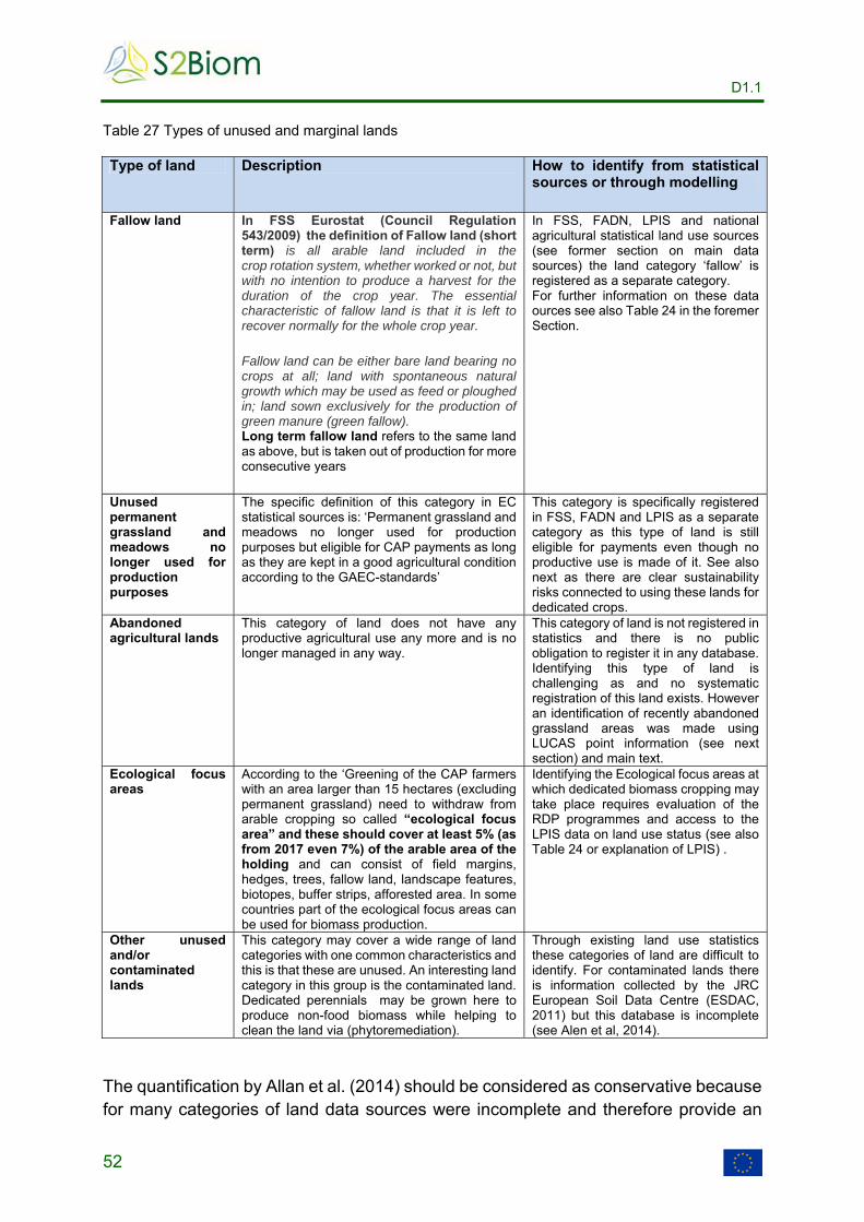
D1.1

52

Table 27 Types of unused and marginal lands

Type of land Description How to identify from statistical sources or through modelling

Fallow land In FSS Eurostat (Council Regulation 543/2009) the definition of Fallow land (short term) is all arable land included in the crop rotation system, whether worked or not, but with no intention to produce a harvest for the duration of the crop year. The essential characteristic of fallow land is that it is left to recover normally for the whole crop year.

Fallow land can be either bare land bearing no crops at all; land with spontaneous natural growth which may be used as feed or ploughed in; land sown exclusively for the production of green manure (green fallow). Long term fallow land refers to the same land as above, but is taken out of production for more consecutive years

In FSS, FADN, LPIS and national agricultural statistical land use sources (see former section on main data sources) the land category ‘fallow’ is registered as a separate category. For further information on these data ources see also Table 24 in the foremer Section.

Unused permanent grassland and meadows no longer used for production purposes

The specific definition of this category in EC statistical sources is: ‘Permanent grassland and meadows no longer used for production purposes but eligible for CAP payments as long as they are kept in a good agricultural condition according to the GAEC-standards’

This category is specifically registered in FSS, FADN and LPIS as a separate category as this type of land is still eligible for payments even though no productive use is made of it. See also next as there are clear sustainability risks connected to using these lands for dedicated crops.

Abandoned agricultural lands

This category of land does not have any productive agricultural use any more and is no longer managed in any way.

This category of land is not registered in statistics and there is no public obligation to register it in any database. Identifying this type of land is challenging as and no systematic registration of this land exists. However an identification of recently abandoned grassland areas was made using LUCAS point information (see next section) and main text.

Ecological focus areas

According to the ‘Greening of the CAP farmers with an area larger than 15 hectares (excluding permanent grassland) need to withdraw from arable cropping so called “ecological focus area” and these should cover at least 5% (as from 2017 even 7%) of the arable area of the holding and can consist of field margins, hedges, trees, fallow land, landscape features, biotopes, buffer strips, afforested area. In some countries part of the ecological focus areas can be used for biomass production.

Identifying the Ecological focus areas at which dedicated biomass cropping may take place requires evaluation of the RDP programmes and access to the LPIS data on land use status (see also Table 24 or explanation of LPIS) .

Other unused and/or contaminated lands

This category may cover a wide range of land categories with one common characteristics and this is that these are unused. An interesting land category in this group is the contaminated land. Dedicated perennials may be grown here to produce non-food biomass while helping to clean the land via (phytoremediation).

Through existing land use statistics these categories of land are difficult to identify. For contaminated lands there is information collected by the JRC European Soil Data Centre (ESDAC, 2011) but this database is incomplete (see Alen et al, 2014).

The quantification by Allan et al. (2014) should be considered as conservative because for many categories of land data sources were incomplete and therefore provide an

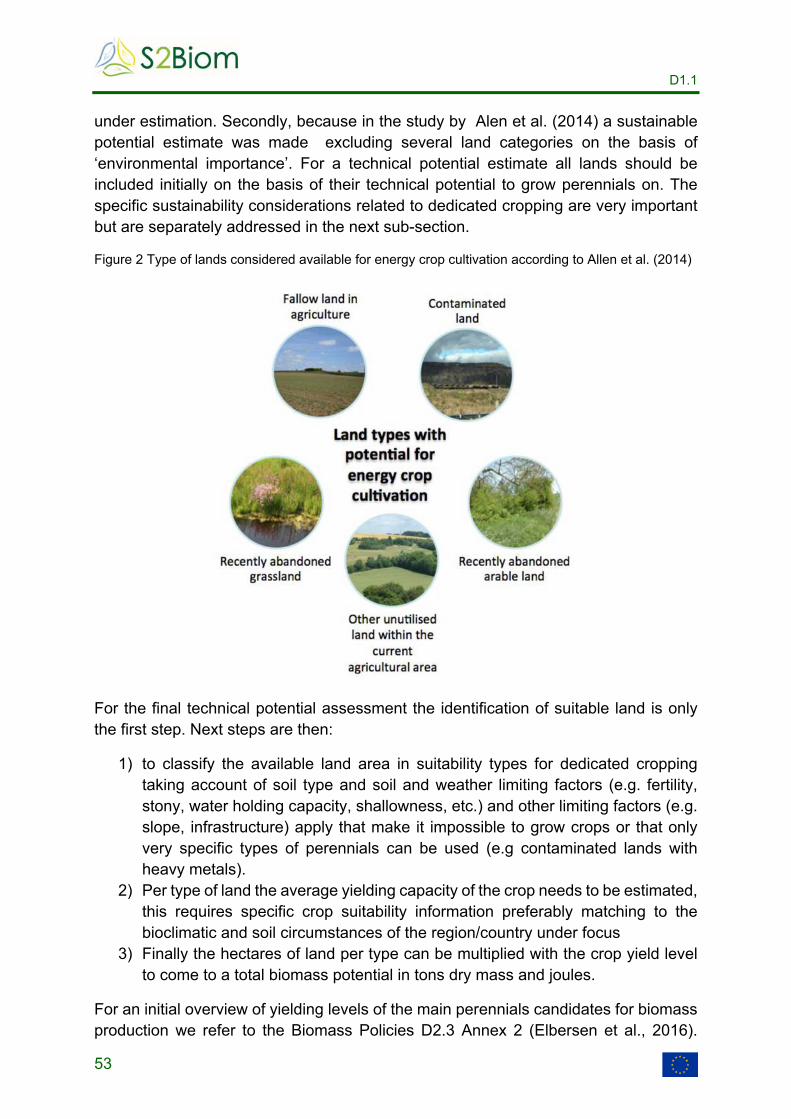
D1.1

53

under estimation. Secondly, because in the study by Alen et al. (2014) a sustainable potential estimate was made excluding several land categories on the basis of ‘environmental importance’. For a technical potential estimate all lands should be included initially on the basis of their technical potential to grow perennials on. The specific sustainability considerations related to dedicated cropping are very important but are separately addressed in the next sub-section.

Figure 2 Type of lands considered available for energy crop cultivation according to Allen et al. (2014)

For the final technical potential assessment the identification of suitable land is only the first step. Next steps are then:

1) to classify the available land area in suitability types for dedicated cropping taking account of soil type and soil and weather limiting factors (e.g. fertility, stony, water holding capacity, shallowness, etc.) and other limiting factors (e.g. slope, infrastructure) apply that make it impossible to grow crops or that only very specific types of perennials can be used (e.g contaminated lands with heavy metals).

2) Per type of land the average yielding capacity of the crop needs to be estimated, this requires specific crop suitability information preferably matching to the bioclimatic and soil circumstances of the region/country under focus

3) Finally the hectares of land per type can be multiplied with the crop yield level to come to a total biomass potential in tons dry mass and joules.

For an initial overview of yielding levels of the main perennials candidates for biomass production we refer to the Biomass Policies D2.3 Annex 2 (Elbersen et al., 2016).

D1.1

54

These initial yield levels calculated using a crop simulation model were elaborated in the Biomass Futures (Elbersen et al., 2012) and ETC-SIA projects (ETC-SIA, 2014). However much relevant work on biomass crop selection and performance is done in S2BIOM. For this it is best to read D1.6 (Dees et al. 2016) and visit the S2BIOM toolset at www.biomass-tools.eu. As part of S2BIOM crop growth simulation the AquaCrop model has been implemented taking account of bioclimatic diversity in Europe. To assess the yield of the biomass crops the data on daily weather factors (are combined in AquaCrop with the phenological characteristics of every biomass crop selected. These factors were derived from a wide range of projects (including from projects in Box 1) and publications on field trial based assessments with lignocellulosic crops under a wide range of soil and climatic circumstances in Europe. For further details see D1.6 (Dees et al. 2017a).

Assessing future technical potentials for perennial biomass crops

Since there is very limited dedicated cropping with perennials already taking place in the EU and the realisation of plantations needs time and will only happen if a clear market demand develops and stimulation measures are taken to start producing these crops it is more useful to assess the future potential for these dedicated crops. This thus requires information on future land use changes particularly in relation to the developments in the categories of land no longer needed for food and feed production and marginal lands as identified above. For identifying these future land use change situations there are generally two approaches to follow:

1) Modelling approaches with models covering all sectors that have a biomass demand and that supply the biomass (e.g. forest, agricultural and other land managing sectors). Ideally it would require a model assessment simulating the production response of the agricultural and forest sector to increased lignocellulosic biomass demand. This however does not exist, not in the least place because there are no models covering all land using and biomass demanding activities in an integrated manner and because there are simply too little reliable data available on types of lands available to cover the real land resources and related production responses in the model.

2) Trend extrapolation and expert judgement to estimate land use change (LUC) and indirect land use change (ILUC) effects

As to modelling we can see that more efforts are being made to incorporate the biomass supply and demand for food, feed, forest biomass and bioenergy in one integrated model. An example is the integrated assessment model GLOBIOM of IIASA which provides useful results at a wider global and European scale in terms of land availability and use. Further examples of the well-known models covering the demand and supply of biomass in one or more sectors are presented in Table 28.

D1.1

55

Table 28 Key models for land availability and cropped biomass potential assessment

Issue(s) Description Type of model Region Holder

Predicting land use changes

CLUE Scanner Land change model, Partial equilibrium. model

Regional Alterra, IVM, VU Amsterdam

Trade policy scenarios

MIRAGE, including biofuel policies, poverty analyses.

computable general equilibrium model, recursive dynamic

multi-country IFPRI, INRA

Macro-economic assessments

MAGNET, including bio-economy, renewable energy policies, agricultural and trade policies.

computable general equilibrium model, recursive dynamic

112 world regions

LEI-WUR

Food security IMPACT, including, agricultural market developments, agricultural policies, technological developments.

Partial equilibrium model, recursive dynamic.

Global IFPRI

Scenario outlooks for agricultural commodity balances

AGMEMOD, scenario outlooks for agricultural commodity balances (including bioethanol and biodiesel) and prices

Partial equilibrium model, recursive dynamic

EU countries, RU, UA, TR, CR,MK, RoW

AGMEMOD consortium (lead vTI and LEI-WUR)

Land allocation and deforestation projections

GLOBIOM, integrating the agricultural, bioenergy and forestry sectors, including biofuel policies, climate change policies.

PEE (Dynamic recursive)

28 world regions IIASA

Market outlooks. Agricultural commodity balances

AGLINK-COSIMO, (including bioethanol and biodiesel) and prices


Global. Over 70 countries and regions worldwide

OECD, FAO

Agricultural commodity balances

CAPRI, (including bioethanol and biodiesel), prices and incomes, environmental indicators

Partial equilibrium model, static

Global. EU: NUTS2, plus 60 other countries and regions

University of Bonn, LEI, Lund uni.,, UPM, JRC-IPTS

Long-term world energy outlooks

POLES Year-by-year recursive, Partial equilibrium model, rec. dyn.

world JRC-IPTS

Agricultural commodity balances

ESIM, (including bioethanol and biodiesel) and prices


Global; individual EU MS, Turkey, USA, Rest-of-the-World-aggregate

University of Hohenheim and vTI

Agricultural supply and incomes

RAUMIS, including , environmental indicators

Supply model Germany (Nuts3-level)

Another option which has been followed in the assessment of future dedicated cropping potentials in this S2BIOM project and also in Biomass Policies is presented in D1.6 (Dees et al. 2017a) and involves a post model assessment. This approach can be seen as a combination of modelling and application of trend extrapolation and expert judgement. Because the identification of land and production response of dedicated crops on more marginal lands is so challenging the post model approach

D1.1

56

aims to first exclude the land resources that are to be used for food and feed production and for the biomass for 1G biofuel generation for which fixed policy targets exist. The land resources that are then ‘left over’ can then be expected to be available in potential for the production of biomass in response to other demands for biomass not covered by the model such as for bioeconomy applications, bioelectricity and heat generation.

All approaches whether model, post-model assessments, extrapolations and expert judgement methodologies, have the same limitations regarding data input. Crucial for making good assessments is the reliable identification of all land categories relevant for the analysis. In relation to agricultural land resources it is clear that lands that in most statistical sources that is an underrepresentation of what can be regarded agricultural land, certainly in relation to recently abandoned lands or common lands that are semi-abandoned but may be good candidates for dedicated perennial cropping activities. As challenging to cover in such analysis are lands that are urban or recreational or semi-natural and that have no productive use or management (any) more.

Sustainability risk and dedicated biomass crops

Sustainability for non-food biomass use, particularly for bioenergy and even more specifically for cropped based biomass resources is an important issue. It is not surprising as biomass demand is a major driver of land use change and related GHG emissions in the future (Laborde, 2011; Searchinger et al., 2008; Al-Riffai et al., 2010; E4tech, 2010; Edwards et al., 2010).

Most critical issues in relation to the environmental sustainability of cropped biomass are (EEA, 2013 & ETC-SIA, 2013):

1) land use change effects and related direct and indirect GHG emissions 2) land use change effects and related biodiversity effects 3) effects on water quality 4) water quantity 5) soil quality effects (soil organic carbon, soil erosion, nutrients)

Basically all these effects are determined by the combination of type of land and soil chosen, the type of crop used and the type of management applied. The effects on biodiversity are determined both by direct uses of land and indirectly by the effects of the cropping activity on the overall environmental quality (soil, water, air).

A) Land use change The cultivation of crops requires land. If an additional demand for crops occurs, for example for the production of biofuels or biochemicals, this may lead to direct (dLUC) and indirect land use changes (iLUC). Direct land use changes occur when:

D1.1

57

1) For the production of this additional crop demand currently productive land (e.g. agricultural land, already used for crop production for food, feed, fuel or fibre, including forest production) is used.

2) The crop is grown on newly converted formally unproductive land (e.g. land without any agricultural or forestry production, such as natural land).

In the first option, the original crop (or other productive land use) would have to be produced elsewhere. This is the starting point for the indirect effects (see Figure 3).

Figure 3 Direct and indirect land use effects (source: EEA, 2013 made by Uwe Fritsche, IINAS)

Firstly, the new demand displaces existing production which needs to be produced elsewhere. This displacement leads directly or indirectly (through a number of other displacement steps) to conversion of natural (e.g. (tropical rain) forests, savannah and wetlands) and semi-natural lands (e.g. extensively grazed grasslands) into agricultural land. Secondly, part of the demand is absorbed through intensification of existing land uses.

The incremental use of land for agricultural production, whether a result of demand for biofuels, food, feed or other non-food applications, leads to an increase of Green House Gas (GHG) emissions and to loss of natural habitats with adverse effects on biodiversity. The extent to which these effects can be related to an extra demand for biofuels or for other non-food uses is difficult to estimate and can only be modeled.

In spite of this ILUC related to demand for bioenergy is critically perceived both in the scientific world as in policy, particularly in the EU and also US. The reason for this is that bioenergy production is stimulated principally to reduce GHG emissions (and related climate change) in the energy and chemical sectors which still have great dependency on fossil feedstock (oil and natural gas). If through the ILUC effects the mitigation potential of bioenergy is diminished or even fully neutralized one can question whether large stimulation of bioenergy production only is advisable.

D1.1

58

To avoid additional GHG emissions through indirect land use effects it is therefore preferred to grow biomass crops on lands that are marginal and abandoned for food and feed production.

B) Biodiversity Converting land to dedicated biomass cropping may lead to additional pressure on (farmland) biodiversity and environmental resources but could as well lead to a decline in pressure as compared to the reference situation. An overview of the main land use change and biodiversity risks of biomass cropping and harvesting is given in ETC-SIA (2013)4 . The summary table of this ETC-SIA study providing an overview of effects of potential land use and land management shifts resulting from biomass cropping on biodiversity is included in the Annex I to the Biomass Policies Deliverable 2.6 (Pelkmans et al., 2015) ‘Guidelines and indicators for the evaluation of sustainable resource efficient biomass value chains’ . In this same report a summary of the main principles determining the biodiversity effects are described in Section 4.2 and will not be repeated here. Basically, the text and table in the Annex 1 of Biomass Policies D2.6 shows that demand for biomass is more likely to have an adverse effect on biodiversity if it leads to a further intensification of land use. However, biomass production sometimes also creates opportunities to extensify and/or diversify land use or introduce minimal management of abandoned habitats where removal of biomass creates opportunities for increasing habitat and species diversity. The effects on biodiversity depends very much on what is taken as the reference. In addition effects also depend on the size of the changes caused by the shift to dedicated biomass crops and the type and presence of rare species their habitats and eventually on an ecosystem’s capacity to provide services. All changes in land use/land cover and land management change that cause the following effects are negative for bodiversity: i) lower species population sizes and composition, ii) invasion of disturbance-adapted species which dominate over rarer and threatened species and iii) overall habitat quality losses through e.g. lower humidity in the soil or lower air moisture, increased pesticide and nitrogen use, and loss of living biomass (e.g. in the case of disruption of (tropical) forests). Effects of biomass crops also depend strongly on the type of crop chosen per situation. Rotational arable crops have higher soil quality requirements and therefore grow on good agricultural lands. Perennial woody and perennial crops can cope with poorer soil quality situations and still produce relatively high biomass yields. In addition, most perennial woody and lignocellulosic crops have a higher GHG efficiency than rotational arable crops since they have lower input requirements and the energy yield per hectare is higher because the full crop is harvested. However, arable crops like sugar beet are

4 ETC/SIA (2013). Review of the EU bioenergy potential from a resource efficiency perspective. Background report to EEA study. Alterra, Wageningen.

D1.1

59

also performing very well in terms of energy yield per hectare because of extremely high sugar yields per hectare, but for other rotational arable crops (e.g. cereals, rape, sunflower) this is not the case and therefore underperform as compared to perennials. Because most woody and lignocellulosic crops have lower soil quality requirements they can well be grown on lower productive land on which they do not compete with rotational arable crops. Acceptable yields can still be reached and displacement effects (i.e. iLUC) are limited. This therefore makes perennials more suitable to be grown on more marginal and abandoned lands. The introduction of perennials biomass crops, particularly in intensive arable lands, may also have positive effects if it leads to a decline in the use of inputs (water, pesticides use, nutrient inputs), increases the landscape structural diversity (provided the changes are not to large scale and the reference biota are not typical open space landscapes supporting birds of prey populations that depend on open landscapes). This may be positive for biodiversity and overall environmental quality, but it also causes displacement of food production. Table 29 Environmental pressures and their link to biodiversity (source: EEA, 2007)

Environmental pressure Link to farmland biodiversity

Erosion Causes a loss of organic soil substances and leads to a loss of habitats. Furthermore, water filtering and buffering functions are reduced with potentially negative effects on biodiversity. Resulting nutrient losses cause eutrophication of surface water affecting wildlife flora and fauna.

Soil compaction Soil structure and other affected soil parameters (air and water household) may lower abundance/diversity of soil biodiversity and wildlife flora.

Nutrient leaching to groundwater and surface water

Cause eutrophication of surface water and soils affecting wildlife flora and fauna (e.g. shift in species) and may also have direct toxic effects on flora and fauna

Pesticide pollution of soils and water

Toxic substances affect flora and fauna directly.

Water abstraction Water abstraction may reduce the ground water level and cause changes in flora and fauna.

Indirect land use change if biomass crops are exchanged for food and feed crops it implies that these crops may need to be cropped somewhere else and this may lead to loss of valuable habitats elsewhere.

Since the effects on biodiversity of biomass cropping are challenging to assess it is best to start from the precautionary principle and ensure that potential adverse effects are avoided. Guideline provided on environmental and related biodiversity risks are provided in the Table 29 which was already presented in the Biomass Policies Deliverable 2.2 and 2.6 but is repeated here. Overall it I clear that analysis for biodiversity impacts per type of crop are determined by a combination of choice of land type, choice of crop and choice of management.

D1.1

60

3.4.3 Data needs, main data sources and modelling requirements

For identifying current land use and cropping patterns there are several statistical and spatial data sources available at EU wide level and at national level. A summary overview of main relevant statistical sources is provided in Table 30.

Table 30 Overview of main EU and international data sources on land use

Name of data source

Type of data collection

Spatial coverage Spatial resolution

Temporal coverage

Temporal resolution

FADN Stratified sample among farms

EU-28 FADN regions

1999 - 2003 (only EU-15) and 2004 - 2010 (EU-27), 2010-.now (EU28)

2/3 yearly

FSS Sample every 2/3 years and full census every 10 years

EU-28 + Norway, Switzerland, Croatia

FSS regions (Nuts 2/3)

For EU-27 from 2003-2007, 2010, 2013 (census). For EU-15 data go back to 1990

2/3 yearly

Eurostat annual crop statistics

National / regional statistics based on surveys

EU-28 National and for some items regional (NUTS1/2)

Starting from 1974 for some MS up to most recent year 2011

Annual

FAOSTAT National statistics Global National 1961 - 2016 Annual

LPIS Farmers survey EU28 (only eligible area which likely excludes large parts of agricultural areas that are semi-abandoned.

Parcel size

1992 - 2016 Annual

LUCAS (point) field sampling

samples in EU-27 countries

Selection of points (±25%) of 2 km grid

Some earlier pilot years, 2009, 2012, …

Every 3 year

UNFCCC Country specific, combination of statistics and Remote Sensing

Annex 1 countries, incl. EU member states, except Malta and Cyprus

National 1990-2010, …. Annual

OECD National statistics OECD countries National 1990-… Annual

GlobCover Satellite derived, but little details on crops as most categories refer to land cover classes.

global 300 m grid cell

2009 Once

GLC2000 Satellite derived, but little details on crops as most categories refer to land cover classes.

global 1 km grid cell

2000 Once

CORINE Land Cover

Satellite derived, but little details on

EU-28 (except Sweden, Finland) +

100 m grid cell

1990-2012, … Every 6 years,

D1.1

61

Name of data source

Type of data collection

Spatial coverage Spatial resolution

Temporal coverage

Temporal resolution

(CLC)1990, 2000, 2006, 2012

crops as most categories refer to land cover classes.

Montenegro, Serbia, Turkey

enables to identify some land abandonment

The best EU wide data source that provides land use information at regional level (Nuts 2 and 3) is the Farm Structure Survey (FSS) and the annual crop statistics. These provide in an EU wide harmonised way data on land use and area (crops) and yield levels.

Other rich data source at national and regional level is the land parcel information system (LPIS) which is the spatial register within the Integrated Administration and Control System (IACS). The IACS ensures that payments of the EU Common Agricultural Policy (CAP) are made correctly. LPIS identifies and quantifies agriculture land for the purpose of targeting CAP payments so it provides for every land parcel the exact land use every year. The IACS/LPIS is operationalized by the paying agencies of each member state. The data is gathered each year through beneficiaries application forms that are filled out by each farmer receiving CAP payments. The advantage of these data is that the detail is high, all crops are covered, but that access to the data (at least at parcel level) is difficult. Another limitation is that not all agricultural land is included s there are countries that do not register land that is not subject to CAP payments. Especially the categories of agricultural lands that are (recently) abandoned are under-represented in this data source, while it is especially this type of land that is of interest for the allocation of dedicated perennial crops. LUCAS data could however be helpful to get some indication of how much and where abandoned lands are.

D1.1

62

3.5 Secondary residues from agriculture

There are several secondary residues produced in the (industrial) processing of agricultural products. In Table 31 an overview is given of such residues and guidelines on how to assess their potential. In the last column specifications are also given on the conventional competing uses known for these residues, as these are often very large and important, making these secondary residues already expense.

For the calculation of the amounts of secondary residues produced, there are 2 options:

1) The area of the crop delivering the residue is multiplied with a residue factor expressing the per hectare delivery of the residue amount (see Table 31, for olive stones)

2) The total yield of the main crop is multiplied with a factor expressing the residue to yield factor (see Table 31)

The overall calculation of the technical potential of secondary residues follows the same general formula as for residues from rotational arable crops:

RESIDUE_YIELDi = AREAi * RES_YIELDi * DM_CONTENTi.

or

RESIDUE_YIELDi = MAIN PRODUCT yieldi * RES_YIELDi ratio * DM_CONTENTi.

Where:

RESIDUE_YIELDi = total residue yield of crop i in Ton/Year dry mass

AREAi = Crop area of crop i RES_YIELDi = Secondary residue yield Ton/Ha/Year in fresh mass of crop i DM_CONTENTi= Dry matter content of residue of crop i MAIN PRODUCT yieldi = this is the yield of the main product i which in the processing at the

mill delivers the secondary by-product

Be aware that for products that are traded internationally and that are therefore not necessarily processed where they are cultivated, like e.g. for cereals (cereal bran), it is more logical to assume that the basis should be the total amount of cereals processed in every country. This implies that cereal bran needs to be calculated for a total net domestic cereal production and imports:

Domestic productioncereals – exportcereals + importcereals

D1.1

63

Table 31 Overview of selection of most common secondary agricultural residues in Europe

Type Definition and how to assess potential?

Calculation factors Competing/ alternative uses

Olive pits Olive pits are a by-product from the olive oil industry. Calculation can be done according to the total area (hectares) of oil olives and the average per hectare yield of olive pits or the residue/main product ratio. The latter requires data on area+average per hectare yield.

Olive pitts make up between 10%-12.5% of the weight of olive according to Garcia et al. 2012 and Pattarra et al., 2010)

Mostly to energy, no alternative uses

Cotton gin residues

The process of cotton ginning produces a by-product composed of bur and stem fragments, immature cottonseed, lint, leaf fragments, and dirt. So-called “cotton gin waste” or trash).

These are residues from the cotton ginning factories.

Calculation can be done according to the total area (hectares) of cotton and the average per hectare yield of the main product and then apply a residue/main product ratio.

*Greece (Nickolaou et al., 2002): 0.1 wet mass residue/main product ratio (wet assuming 13% moisture)

Animal feed, compost

Cereal bran These are residues from the flour mills. Calculation can be done according to the total area (hectares) of cereals used for flouwer production and the average per hectare yield of the main product and then apply a residue/main product ratio.

*Portugal (Diaz & Azevedo, 2004): for rye 0.3 wet mass residue/main product ratio (wet assuming 12.5% moisture). For wheat flower the ratio is 0.19 (13 % moisture) and for maize flower the reatio is 0.2 (18% moisture)

Animal feed

Rice husk These are residues from the rice mills.

Calculation can be done according to the total area (hectares) of rice and the average per hectare yield of the main product and then apply a residue/main product ratio.

*Greece (Nickolaou et al., 2002): 0.16 wet mass residue/main product ratio (wet assuming 10% moisture)

Animal feed

Soy bean, sunflower and rape seed oil residues

These are residues from the vegetal oil industries. Calculation can be done according to the total area (hectares) of rice and the average per hectare yield of the

*Portugal (Diaz & Azevedo, 2004): for sunflower 0.6 wet mass residue/main product ratio (wet assuming 10% moisture). For rape the ratio is ..... (....

Animal feed

D1.1

64

Type Definition and how to assess potential?

Calculation factors Competing/ alternative uses

main product and then apply a residue/main product ratio.

% moisture) and for soybean the ratio is 0.8 (13% moisture)

Nut peelings (walnut, almond, hazelnut)

These are secondary residues from the peeling plant for nuts. Calculation can be done according to the total area (hectares) of nut trees and the average per hectare yield of the main product and then apply a residue/main product ratio.

*Greece (Nickolaou et al., 2002): 0.95-1.5 wet mass residue/main product ratio (wet assuming 5%-8% moisture)

Mostly to energy, compost

Beer dregs Residues from the beer factories of which the main is the brewer’s spent grain (85% of residues). Others are hot trub, residual years & diatomaceous earth slurry

For every 100 kg of grain input 125 kg of wet spent grain (bagasse) is produced (80% moisture). Or for every 10 liters of beer 14-20 kg of wet spent grain is produced (see Dos Santos-mathias et al., 2014).

Animal feed, other chemical uses

Pressed grapes dregs

These are secondary residues from the vine industry. Calculation can be done according to the total area (hectares) of vineyards and the average per hectare yield of the main product and then apply a residue/main product ratio.

*Portugal (Diaz & Azevedo, 2004): 0.19 wet mass residue/main product ratio (wet assuming 80% moisture)

Compost

Fruit juice dregs (oranges and other citrus)

The secondary residues from the juice industry. Calculation can be done according to the total area (hectares) of citrus (going to fruit juice production!) and the average per hectare yield of the main product and then apply a residue/main product ratio.

*Portugal (Diaz & Azevedo, 2004): 0.56 wet mass residue/main product ratio (wet assuming 80% moisture)

Sugar beet industry residues (pulp & molasses)

Residues from the sugar mill. Calculation can be done according to the total area (hectares) of sugarbeet and the average per hectare yield of the main product and then apply a residue/main product ratio.

About 76% of the sugarbeet ends up as pulp in the sugar mill process.

Animal feed

Potatoe industry residues

Residues from the potatoe processing industry. Calculation can be done according to the total area (hectares) of potatoes converted to starch and feed the average per hectare yield of the main product and then apply a residue/main product ratio. Main residues concern potatoe peels and press fibre

About 15% of the processed potatoes (towards chips, crisps and starch) consists of peels.

The extraction of starch from strach potatoes into potatoe flour delivers press fibre which is estimated to amount to 15% of the input (e.g. 150 kg/ton potatoe input). The press fibre consists for 83.5% of moisture (Elbersen et al., 2011).

Animal feed

D1.1

65

As for data availability we refer to the same data sources as discussed in former sections on primary agricultural residues.

3.6 Biomass from other land categories then forest and agricultural lands


There are many biomass sources that can be assessed from the other land uses category such as grassland cuttings from nature protection areas, recreational areas, dykes and from road side verges. The woody biomass potentials can also come from road side verges and from landscape maintenance. Properly assessing their quantities requires a lot of high resolution data not only on the land use and land cover classes, but also on the type of vegetation present to make a proper estimate of the amount of biomass produced and the cutting and wider management requirements and practices and management and ownership structure.

Because of the lack of high resolution data, particularly in relation management practices and vegetation types/species distribution and limited time to invest in collection of data the focus in S2BIOM was only on the road side verge grassland potential and the approach to assessing it is presented here.


The assessment of potential biomass from road side verges builds on the assessments already done as part of the Biomass Futures (Elbersen, et al.,2012) and Biomass Policies (Elbersen et al., 2016) projects and the results of this assessment were further refined and extrapolated to 2012, 2020 and 2030 in S2BIOM, see Deliverable 1.6 (Dees et al. 2017a) for details.

The main information and data sources required are presented in Table 32 underneath. The largest challenge is to understand what roads are bordered by grasslands and how wide the grassland verge is. Since it is impossible to know this exactly a rough estimate needs to be made. A 10 meter boundary was assumed in the S2BIOM and Biomass Policies assessment of road side verges. To make an appropriate estimate of the width at local area more one can use aerial photographs (AEROGRID) and Google Maps. This however can be very time consuming when a representative coverage needs to be estimated over a large space. It is proposed to then use some sampling framework before collecting the point information.

D1.1

66

Table 32 Example of information and possible data sources to calculate the road side verge grassland potential

Item Description Data sources suggested Road networks Road network information is

required to calculate the length of the roads in every region.

National road network data, EU-wide road network map (ESRI roads (Europe Roads represents the roads (European Highway System, national, and secondary roads) and de roads network database, Eurostat 2010)

Road side verge width An average width needs to be estimated for the verge of grassland along the road

Aerial photographs (AEROGRID) and Google Maps

Grass biomass production To calculate the total potential the area of grassland verges needs to be multiplied with the yearly grassland biomass production. Since it concerns unfertilised grasslands it is important to identify information on unproductive grasslands per climatic zone covered

Smidt et al., 2008

For the estimation of the grassland yield Smit et al. (2008) is a good source. In this study average grassland productivity factors for different types of grassland per environmental zone in Europe were assessed. The type of grassland used in this map was assumed to be the most extensive grassland type assuming no fertilisation and poor soils. The environmental zonation ensures that grassland productivity is directly linked to climatic factors such as rainfall, evapotranspiration and length of growing season (Metzger et al., 2006).

3.7 Biomass from waste


In this report we focus on two relevant waste biomass categories, namely biowaste and post-consumer wood.

3.7.1.1 Biowaste

Biowaste is defined as “biodegradable garden and park waste, food and kitchen waste from households, restaurants, catering and retail premises and comparable waste from food processing plants” (Waste Framework Directive (2008/98/EC)). Biowaste is part of biodegradable municipal waste as defined in the landfill Directive (99/31/EC), but it excludes textile and separately collected paper and paperboard. Biowaste can be separately collected or be part of integrally collected municipal waste. Separately

D1.1

67

collected biowaste can generate energy by anaerobic digestion followed by composting. Integrally collected biowaste can be incinerated with energy generation, or part of the biowaste can be separated as part of “refuse derived fuel” and subsequently combusted in a bioenergy plant. The choice for separate or integral collection of biowaste strongly depends on the waste policy of the country. In case of biowaste no difference has been made between the technical potential and sustainable potential as all collected waste is in principle available for energy generation, i.e. biogas production before composting in case of separate collected biowaste and incineration with energy recovery or RDF combustion in case of biowaste as part of integrally collected waste.

3.7.1.2 Post-consumer wood

Post-consumer wood (PCW) includes all kinds of wooden material that is available at the end of its use as a wooden product (“post-consumer” or “post-use” wood). Post-consumer recovered wood mainly comprises packaging materials (e.g. pallets), demolition wood, timber from building sites, and fractions of used wood (e.g. used wooden furniture) from residential, industrial and commercial activities. Post-consumer wood is a tertiary raw material, which should be collected, sorted, re-utilised or recycled, and finally used for energy production. The technical potential assumes that all collectable post-consumer wood is available for energy generation. About 5% of available post-consumer wood cannot be recovered for technical reasons. The sustainable potential shows the potential for energy generation, taking into account the current use of post-consumer wood for material applications, currently mainly particleboard production. Obviously, the sustainable potential is in most cases much lower than the technical potential, as the latter does not take into account current material use of post-consumer wood.


3.7.2.1 Biowaste

The availability of biowaste in year x on NUTS3 level can be established as:

MSW generated per capita (kg/capita) x

biowaste fraction (%) x

population of the NUTS3 area (persons).

A further distinction is made between the separately collected biowaste and biowaste as part of mixed waste.

MSW per capita

It is likely that differences exist in quantities of MSW per capita between regions and that the composition differs between urban and rural areas, etc. Therefore, if possible regional statistics (NUTS 3, 2 or 1) should be applied. If no regional data is available,

D1.1

68

national data can be used, which is available at the national statistical offices as well as in Eurostat. Eurostat provide information on the amounts of municipal solid waste generated per capita in a country (See Municipal waste generation and treatment, by type of treatment method, code tsdpc240, http://epp.eurostat.ec.europa.eu/tgm/table.do?tab=table&init=1&plugin=1&language=en&pcode=tsdpc240). The data is available on country level (NUTS0). Eurostat has carried out a pilot on collection data on Municipal waste per capita by NUTS 2 regions (See Municipal waste by NUTS 2 regions - pilot project, Eurostat code: env_rwas_gen). The project covers, however, a limited number of countries and data collection has stopped after 2011.

Biowaste fraction

The biowaste fraction of municipal solid waste can be collected from sorting analyses on national or if possible regional or site level. Arcadis and Eunomia (2010) have analysed literature on the share of biowaste in household waste in all the EU27 countries. In case no data could be found for a particular country, the study used the share of biodegradable municipal waste in municipal waste that is known for the year 1995 because of the implementation of the Landfill directive, multiplied with a factor of 56% biowaste in biodegradable municipal waste. The latter factor is based on composition of household waste in Pleven and Flanders and the assumption that total biodegradable waste consists of biowaste + paper + textiles + ½ of other fractions. The biowaste fractions established in Arcadis and Eunomia (2010) are used in S2BIOM as it forms the most up to date complete set of biowaste fractions for the EU27 currently available. For Croatia (the 28th EU country) BTG has assumed that the biowaste fraction is the average fraction of neighbouring countries Slovenia and Hungary. For the non-EU countries, no data on the biowaste fraction has been collected, instead the average biowaste fraction of 35.9% as established in Arcadis and Eunomia (2010) has been used.

Population data

For a year in the past population data on NUTS3 level can be taken from Eurostat (code demo_r_gind3), or national statistics. Projections on the development of the total quantity of biowaste are assumed to be proportional to population growth. The main scenario on population development from Eurostat has been used to predict the population in 2020 (Eurostat code proj_13npms). This information is only available on country level (NUTS0). If national or regional statistics are available on population growth at higher NUTS levels (NUTS1-3), this data is preferred. If only NUTS0 information is available, in order to establish population data in 2020 and 2030 the NUTS3 level population data of year x needs to be multiplied with the expected change in population in 2020 and 2030 (or any other year in the future) compared to year x on national level.

The development of biowaste availability has not been linked to GDP growth, given the uncertainty of GDP development and the fact that many EU countries will reach or

D1.1

69

have reached decoupling with GDP. This is a conservative assumption, especially for European countries with still a relatively low GDP.

Separately collected biowaste versus biowaste in mixed waste

Arcadis and Eunomia (2010) have analysed the percentages of biowaste that is collected separately or exist as part of mixed waste for the EU27 on country level. These numbers (base year 2008) were used in S2BIOM. In Arcadis and Eunomia (2010) also projections have been provided of the shares of biowaste going to the different treatment options like landfill, incineration, MBT5, composting, backyard composting, anaerobic digestion and others have been made for the years 2008-2020. It has been assumed that all countries meet the requirement of the landfill directive, e.g. that maximally 35% of the amount of biodegradable waste generated in base year 1995 is landfilled in 2020, even if current developments show that diversion from landfill has not been successful yet. Furthermore, the projections are based on policy views and current changes in treatment of biowaste in the member state concerned. For instance, some countries have a strong preference for MBT, others for incineration with energy recovery. For the year 2030 the same shares between treatment options are used as in the year 2020, as currently no policies are known that influence the production of biowaste after 2020.

Conversion factors

The following table provides conversion factors that can be used to convert the mass to volumes and energy. The data has been retrieved from the biomass properties database developed in WP2 of S2BIOM.

NVCar MJ/kg

Moisture content (w%ar)

Basic density kg/m3

Biowaste as part of integrally collected municipal waste: Biodegradable waste of not separately collected municipal waste (excluding textile and paper)

10.8 27.2% 500

Separately collected biowaste: Biodegradable waste of separately collected municipal waste (excluding textile and paper)

4.3 55.6% 500


At European level no complete statistical information on amounts of post-consumer wood, including (1) packaging wood, (2) construction and demolition wood and tertiary wood from households, companies and (3) fractions of used wood (e.g. used wooden furniture) from residential, industrial and commercial activities are difficult to find. Detailed Eurostat information can be found on packaging wood waste. Eurostat also gives data on “wood waste”, but this includes not only post-consumer wood but processing wastes from agriculture forestry and fishing sectors. Because of this

5 Mechanical Biological Treatment

D1.1

70

mixture of secondary wood processing and tertiary post-consumer wood within one category, Eurostat data cannot be used to determine the potential of post-consumer wood. Regional end users are advised to check national statistics that might contain more detailed information on post-consumer wood than Eurostat. Most likely, additional data will need to be collected from literature or from primary research, i.e. direct collection of data from the main demolition wood processors in a region, such as waste processing companies, local particle board producers and bioenergy producers.

In S2BIOM, data on post-consumer wood was obtained from forest biomass resource assessments done for the EUwood and EFSOS II studies (Mantau et al. 2010; UN-ECE/FAO 20116). EUwood combines among others Eurostat and COST Action E31 data. The EFSOS II data on demolition wood is based on EU wood, but covers Europe as a whole instead of EU28. In order to determine the base potential PCW available for energy, it is necessary to estimate how much is used for material applications. In the Methodology report of the EUwood project7, a table is given on the availability of PCW material [for material recycling] and PCW energy for 2007, page 119-120, which have been used in S2BIOM as well.

The potential can be described as follows:

PCW technical potential = PCW material + PCW energy + PCW disposed PCW sustainable potential = PCW energy + PCW disposed

in which: PCW material = PCW used for materials like panels and chipboards PCW energy = PCW used for energy production PCW disposed = landfilled and/or incinerated with MSW.

In S2BIOM, the current percentages of waste wood used in material applications, energy generation and landfilled are based on the above-mentioned studies, e.g. EU Wood and EFSOS II. In case of estimation of the future sustainable potential of post-consumer wood, one could also take into account relevant policy developments. For instance, The Circular Economy Package proposes a target of 75% of material recycling of packaging wood in 2030, this will be a challenge but the quality of packaging waste (mainly clean sawn wood) is suitable for recycling. The other waste wood fractions are more difficult to recycle; there are not too many options to recycle used panels (particle board, MDF, OSB, plywood). Recycling rates of other wood (besides packaging) are not expected to exceed 50%. Moreover, given the quality requirements for material applications of wood, all hazardous waste wood can be assumed to be available for energy generation.

6 UNECE (United Nations Economic Commission for Europe), FAO (Food and Agricultural Organization of the United Nations) 2011: The European Forest Sector Outlook Study II; Geneva 7 EU Wood (2010) Methodology report, real potential for changes in growth and use of EU forests EUwood. Call for tenders No. TREN/D2/491-2008.

D1.1

71

Distinction between hazardous versus non-hazardous wood

Eurostat differs between hazardous and non-hazardous wood, but unfortunately does not have a separate category for post consumer wood, but includes also processing wastes from agriculture, forestry and fishing sectors as part of wood waste. It will be necessary to collect data on the percentage hazardous wood on country level. For instance, according to Probos (2014)8 in the Netherlands yearly around 1000-1400 ktonnes A/B wood and 80-120 ktonnes/year of hazardous C-wood9 is produced in the period 2007-2012. This means that hazardous C-wood counts for 7.6% (7.4-7.8%) of total post consumer waste. According to a dedicated case study in the Bioxchange project, in Germany 17% of the PCW is hazardous. According to the same study in the Netherlands the share is lower, only 6%10.

Conversion factors

The following table summarises conversion factors that can be used to convert mass to volumes and energy. The data has been retrieved from the biomass properties database developed in WP2 of S2BIOM.

NVCar

MJ/kg

Moisture content

(w%ar)

Basic density

kg/m3 Hazardous post consumer wood 14.2 13.9% 500 Non hazardous post consumer wood 16 13.1 500

3.7.3 Data needs, main data sources and modelling requirements

3.7.3.1 Biowaste

While statistical information is available on the production of municipal solid waste, in case of integrally collected municipal waste, the percentage of biowaste has to be determined by waste composition analysis. The existing biowaste collection

8 De markt van resthout en gebruikt hout in 2012, Bosberichten 2014-04 (in Dutch) 9 Three main categories of post consumer wood can be distinguished, following the Dutch national Land Use Plan9: A-quality: unpainted and untreated wood; B-quality: wood not mentioned under A-wood and C-wood: among others painted, lacquered and glued wood. A-quality wood can be recycled or used for material recycling. B-quality wood can be used for both applications as well, given that certain treatment is provided (removing paint) or emission reduction equipment. A- and B-quality wood are often provided as mixtures, therefore it is not possible to distinguish between both categories in statistics. Both qualities will be indicated as non-hazardous wood. C-quality (hazardous) consists of treated wood like: Wood treated with creosotes, wood treated with wood preservatives containing copper, chrome and arsenic (CC and CCA wood), wood treated with other means (fungicides, insecticides, etc.).C-wood is a distinct category, in general not suitable for material recycling (with the exception of material reuse of creosoted wood), but in general9 this wood can be combusted for energy generation, provided that sufficient measures are taken, especially advanced emission reduction measures.

10 Mark van Benthem, Nico Leek, Udo Mantau, Holger Weima; Markets for recovered wood in Europe: Case studies for the Netherlands and Germany based on the Bioxchange project

D1.1

72

infrastructure determines the possibilities for bioenergy generation, i.e. separately collected biowaste could be anaerobically digested for biogas production before composting; integrally collected biowaste can be incinerated or the RDF fraction could be combusted separately. In any regional analysis, it is necessary to take into account the existing infrastructure and contracts. At certain critical moments, after the contract period of a municipality with a waste processor (typical 10 years), the municipality or region has the possibility to direct the biowaste to a processor that produces bioenergy production in its facility. The data at national level can help to estimate the total possible impact of energy generation with biowaste, however, the existing infrastructure and the national waste management plans determine for a large part the realisation of the energy potential of biowaste in a region.


In order to make an estimation of post-consumer wood including used packaging wood, construction and demolition wood, and other waste wood from households and companies (like used furniture), it is necessary to combine statistical information with sector studies and other literature. For instance, a number of countries have statistical information available on the fractions of post-consumer wood collected at household level. In some countries like Germany and the Netherlands detailed wood flow analyses have been carried out. Consultancies provide waste wood potential estimations, etc. A major step forward would be if Eurostat would further specify and categorise “waste wood”, and make a distinction between secondary industrial wood waste and post consumer wood. An additional challenge to obtain the sustainable potential is the determination of the fraction of the wood that is suitable and used for material applications. This requires a detailed study of the actual wood flows in the country of region concerned, as this cannot be found in national statistics.

D1.1

73

4 Main recommendation and conclusions

With this guideline recommendations are made available that allow the estimation of the major biomass categories on regional level by making use of approaches that are developed and designed for assessments at European scales and that can also be utilised for regional assessments. It is for all categories recommended to clarify the availability of regional data and knowledge on factors that are utilised in the estimation formulae. Regionally available information may also allow the utilisation of methods that can provide more accurate estimates. It is thus recommended to explore if regional approaches can be applied and to consider otherwise the methods and data sources described in this report. Furthermore, it needs to be emphasised that both methodologies and data collection at European scale is still subject to research and improvement and it is thus further recommended to consider these advancements as well.

D1.1

74

5 References

Allen, B., Kretschmer, B., Baldock, D., Menadue, H., Nanni, S., & Tucker, G. (2014). Space for energy

crops – assessing the potential contribution to Europe’s energy future. Report produced for

BirdLife Europe, European Environmental Bureau and Transport & Environment., (May), 69.

Al-Riffai P., Dimaranan B., Laborde D. (2010) Global Trade and Environmental Impact Study of the EU

Biofuels Mandate, IFPRI.

Arcadis and Eunomia (2010) Assessment of the options to improve the management of bio-waste in

the European Union - final report, Version C 12-02-2010. Study contract Nr.

07.0307/2008/517621/ETU/G4, European Commission, DG Environment

Britz and Witzke, 2012. CAPRI model documentation 2012. http://www.capri-

model.org/docs/capri_documentation.pdf

CEPI, Germany (2012) Consumption of Pulpwood in the Pulp and Paper Industry.

CEPI, Germany (2014) Consumption of Pulpwood in the Pulp and Paper Industry.

CEPI (2015) Historic Statistics 1991 – 2014.

CGIAR, 2012 (eco-crop suitability index)

Coleman, K. and Jenkinson, D.S. 1999. RothC-26.3 - A Model for the turnover of carbon in soil: Model

description and windows users guide: November 1999 issue. Lawes Agricultural Trust

Harpenden. ISBN 0951445685.

Dees, M., Bodo, B., Panoutsou, C., Böttcher, H., Duchossois, G., Eleftheriadis, G., Gunia, K., Gyuris,

P., Hirschmugl, M., Kajba, D., Kalaitzidis, C., Keuck, V., Koch, B., Köppen, S., Kunikowski, G.,

Lakyda, P., Lindner, M., Pace, G., Ramos, I., Rettenmaier, N., Rosillo -Calle, F., Schardt, M.,

Smeets, E., T orén, J., Vasylyshyn, R., Vis, M., Wirsenius, S., Zhelyezna, T. (2012): Status

and future of biomass assessment for energetic use in Europe. In, Proceedings oft he 20th

European Biomass Conference and Exhibition, Milano, Session 1AO.6.1 , 23 –34

Dees, M., Elbersen, B., Fitzgerald, J., Vis, M., Anttila, P., Forsell, N., Ramirez-Almeyda, J., García

Galindo, D., Glavonjic, B., Staritsky, I., Verkerk, H., Prinz, R., Monti, A., Leduc, S., Höhl, M.,

Datta, P., Schrijver, R., Sergey Zudin, Lindner, M., Lesschen, J. & Diepen, K. (2017a): A

spatial data base on sustainable biomass cost-supply of lignocellulosic biomass in Europe -

methods & data sources. Project Report. S2BIOM – a project funded under the European

Union 7th Frame Programme. Grant Agreement n°608622. Chair of Remote Sensing and

Landscape Information Systems, Institute of Forest Sciences, University of Freiburg. 173 p.

Dees, M., Elbersen, B., Fitzgerald, J., Vis, M., Anttila, P., Forsell, N., Datta, P., Staritsky, I., Glavonjic,

B., Verkerk, H., Prinz, R., Leduc, S., Datta, P., Lindner, M., Höhl, M. (2017b) Atlas with

regional cost supply biomass potentials for EU 28, Western Balkan Countries, Moldavia,

Turkey and Ukraine. Project Report. S2BIOM – a project funded under the European Union

7th Frame Programme. Grant Agreement n°608622. Chair of Remote Sensing and Landscape

Information Systems, Institute of Forest Sciences, University of Freiburg.

E4tech. (2010) A causal descriptive approach to modelling the GHG emissions associated with the

indirect land use impacts of biofuels. Final report, E4tech, London.

EC 2011. Regions in the European Union - Nomenclature of Territorial Units for Statistics NUTS

D1.1

75

2010/EU-27. Luxembourg.

EC. 2009. Natura 2000 Sites, Version January 2009. Brussels: EC – DG Environment.

Edwards, R.A.H. Šúri, M. Huld, M.A. Dallemand, M.A. (2005). GIS-Based Assessment of Cereal Straw

Energy Resource in the European Union; Proceedings of the 14th European Biomass

Conference & Exhibition; 17-21 October 2005, Paris

EEA (2013). EU Bioenergy potential from a resource efficiency perspective. EEA report no.6/2013

Elbersen B.S. & Staritsky, I. (2016). Guidelines for data collection to estimate and monitor technical

and sustainable biomass supply. Deliverable 2.2 of the Biomass Policies project.

Elbersen B.S. & Staritsky, I. (2016). Guidelines for data collection to estimate and monitor technical

and sustainable biomass supply. Deliverable 2.2 of the Biomass Policies project.

Elbersen, B., I. Staritsky, G. Hengeveld, M.J. Schelhaas, H. Naeff, H. Böttcher 2012. Atlas of EU

biomass potentials. Deliverable 3.3: Spatially detailed and quantified overview of EU biomass

potential taking into account the main criteria determining biomass availability from different

sources. Biomass Futures.

http://www.biomassfutures.eu/work_packages/WP3%20Supply/D_3_3__Atlas_of_technical_a

nd_economic_biomass_potential_FINAL_Feb_2012.pdf

Elbersen, B.S.; Staritsky (2012). Spatially detailed and quantified overview of EU biomass potential

taking into account the main criteria determining biomass availability from different sources.

Report for Task 3 in Biomass Futures project. IEE 08 653 SI2. 529 241.

Elbersen, B.S.; Staritsky, I., Hengeveld G. &; Lesschen, J.P. (2016). Outlook of spatial biomass value

chains in EU28. Deliverable 2.3 of the Biomass Policies project.

Elbersen, B.S.; Staritsky, I., Hengeveld G. &; Lesschen, J.P. (2016). Outlook of spatial biomass value

chains in EU28. Deliverable 2.3 of the Biomass Policies project.

Elbersen, W., Janssens, B. & Koppejan, J. (2011). De Beschikbaarheid van biomassa voor energie in

de agro-industrie. Report 1200. Wageningen UR Food & Biobased Research.

ETC/SIA (2013). Review of the EU bioenergy potential from a resource efficiency perspective.

Background report to EEA study. Alterra, Wageningen. European Commission.

ETC/SIA, 2013. Review of the EU bioenergy potential from a resource efficiency perspective.

Background report to EEA study. Alterra, Wageningen.

European Central Bank 2013. Press Release. Euro Area MFI Interest Rate Statistics: December 2013.

1 February 2013. 10 p. Available at: http://www.ecb.europa.eu

European Soil Database 2006. (v. 2.0), Raster Version 1 km×1 Km. Ispra: EC – DG Joint Research

Centre.

EuroPruning (2015). Mapping and analysis of the pruning biomass potential in Europe. Deliverable

report D3.1. Available at: www.europruning.eu

EuroPruning (2016). Report on environmental evaluation of the supply chain. EuroPruning Deliverable

report D8.1. - Available at: www.europruning.eu

Eurostat. 2011. “Statistical Database of the European Union.”

EUROSTAT. 2015a. Purchasing power parities (PPPs), price level indices and real expenditures for

ESA2010 aggregates [prc_ppp_ind] Internet site. Available at:

D1.1

76

http://ec.europa.eu/eurostat/cache/metadata/en/prc_ppp_esms.htm. Accessed 4th November

2015]

EUROSTAT. 2015b. Labour cost, wages and salaries (including apprentices) - NACE Rev. 2

[lc_ncostot_r2]. Internet site. Available at:

http://ec.europa.eu/eurostat/cache/metadata/en/lcs_esms.htm. [Accessed 15th April 2015]

experts consultation – Pamplona, 18-19 October 2006, In: Joint Research Centre of the European

Commission IES JRC and CENER, National Renewable Energy Centre of Spain (2006).

,Proceedings of the Expert Consultation. “Cereals Straw Resources for Bioenergy in the

European Union”. Pamplona 2006. EUR 22626 2007. Available at:

http://iet.jrc.ec.europa.eu/remea/events/cereals-straw-resources-bioenergy-european-union

FP7 GRANT AGREEMENT N˚: 213417

García-galindo, D, Gómez-palmero, M, Pueyo, E, Germer, S., Pari, L., Afano, V., Dyjakon, A.,

Sagarna, J., Rivera, S., Poutrin, C. (2016). Agricultural pruning as biomass resource:

generation, potentials and current fates. An approach to its state in Europe. European

Biomass Conference & Exhibition 2016

Haynes, R.J., Goh, K.M. 1980. Variation in the nutrient content of leaves and fruit with season and

crown position for two apple varieties. Australian Journal of Agricultural Research 31(4): 739-

748. 1980.

Heinimö & Alakangas (2011) Market of biomass fuels in Finland 2009.

Hill A., Rewald B., Rachmilevitch S.: Belowground dynamics in two olive varieties as affected by saline

irrigation. Scientia Horticulturae 162 (2013), 313-319.

IIASA/FAO, (2012) Agro-climatic potential database

Inglese, P, Caruso, T., Gugliuzza, G. 2002. Crop load and rootstock influence on dry matter

partitioning in trees of early and late ripening peach cultivars. Journal of the American Society

for Horticultural Science. Vol.127(5): 825-830. 2002.

Inglese, P, Caruso, T., Gugliuzza, G., Pace, L.S. 2001. The effect of crop load and rootstock on dry

matter and carbohydrate partitioning in peach trees (Prunus persica batsch). Acta

Horticulturae 557: 447-455. 2001.

Joint Research Centre of the European Commission IES JRC and CENER, National Renewable

Energy Centre of Spain (2006). ,Proceedings of the Expert Consultation. “Cereals Straw

Resources for Bioenergy in the European Union”. Pamplona 2006. EUR 22626 2007.

Kindermann, G., Obersteiner, M., Sohngen, B., Sathaye, J., Andrasko, K., Rametsteiner, E.,

Schlamadinger, B., Wunder, S., Beach, R., 2008. Global cost estimates of reducing carbon

emissions through avoided deforestation. Proceedings of the National Academy of Sciences

105, 10302-10307.

Kindermann, G., Schorghuber, S., Linkosalo, T., Sanchez, A., Rammer, W., Seidl, R., Lexer, M., 2013.

Potential stocks and increments of woody biomass in the European Union under different

management and climate scenarios. Carbon Balance and Management 8, 2.

Klima activ (2014a) Wood flows in Austria.

http://www.klimaaktiv.at/english/renewableenergy/woodflowsaustria.html

D1.1

77

Klima activ (2014b) Spreadsheet for the calculation of parameters and prices of wood fuel

assortments. www.klimaaktiv.at.

Laborde, D. 2011. Assessing the land use change consequences of European biofuel policies. Final

report ATLASS consortium. Contract no. TRADE/07/A2; Washington DC: IFPRI

http://trade.ec.europa.eu/doclib/docs/2011/october/tradoc_148289.pdf (accessed 1 July 2012)

Lesschen, J.P., van den Berg, M., Westhoek, H.J., Witzke, H.P., Oenema, O., 2011. Greenhouse gas

emission profiles of European livestock sectors. Animal Feed Science and Technology 166–

167, 16-28.

Mantau, U. Saal, U., Prins, K., Steierer, F., Lindner, M., Verkerk, H., Eggers, J., Leek, N.,

Oldenburger, J., Asikainen, A., Anttila, P. 2010: EUwood - Real potential for changes in growth

and use of EU forests. Methodology report. Hamburg/Germany, June 2010. 165 p.

Mantau, U.;BilitewskiI (2010):Stoffstrom-Modell-Holz:Rohstoffströme und CO2-Speicherung in der

Holzverwendung.Celle:Forschungsbericht für das Kuratorium für Forschung und Technik des

Verbandes der Deutschen Papierfabriken e.V.(VDP),77 S.

Metzger, M.J., Bunce, R.G.H., Jongman, R.H.G., Mücher, C.A., Watkins, J.W., 2005. A climatic

stratification of the environment of Europe. Global Ecology and Biogeography 14, 549–563.

Monforti, F., Lugato, E., Motola, V.,Bodis, K., Scarlat, N. & Dallemand, J-F (2015). Optimal energy use

of agricultural crop residues preserving soil organic carbon stocks in Europe. Renewable and

sustainable Energy Reviews 44 (2015), 519-529.

Nabuurs, G., Pussinen, A., van Brusselen, J., Schelhaas, M., 2007. Future harvesting pressure on

European forests. European Journal of Forest Research 126, 391–400.

Packalen T, Sallnäs O, Sirkiä S, Korhonen K, Salminen O, Vidal C, Robert N, Colin A, Belouard T,

Schadauer K, Berger A, Rego F, Louro G, Camia A, Räty M, San-Miguel-Ayanz J, 2014. The

European forestry dynamics model: concept, design and results of first case studies.

Publications office of the European Union.

Panoutsou and Labalette (2007), Cereals straw for bioenergy and competitive uses, JRC

Parton, W.J., Schimel, D.S., Cole, C.V., Ojima, D.S., 1996. Analysis of factors controlling soil organic

matter levels in Great Plains grasslands. Soil Sci. Soc. Am. J. 51, 1173–1179.

Pattara et al. / Renewable and Sustainable Energy Reviews 14 (2010) 1484–1489.

Pelkmans et al., (2015). Biomass Policies Deliverable 2.6 () ‘Guidelines and indicators for the

evaluation of sustainable resource efficient biomass value chains’

Pilli, R., Grassi, G., Kurz, W.A., Smyth, C.E., Blujdea, V., 2013. Application of the CBM-CFS3 model to

estimate Italy's forest carbon budget, 1995–2020. Ecological Modelling 266, 144-171.

Pilli, R., Grassi, G., Kurz, W.A., Viñas, R.A., Guerrero, N.H., 2016. Modelling forest carbon stock

changes as affected by harvest and natural disturbances. I. Comparison with countries’

estimates for forest management. Carbon Balance and Management 11, 1-18.

Pitacco A., Meggio F.: Carbon budget of the vineyard. A new feature of sustainability. EDP Sciences,

BIO web of conferences 5 (2015), 01024.

Poulson, D.S., Glendining, M.J., Coleman, K., Whitmore, A.P., 2011. Implications for Soil Properties of

Removing Cereal Straw: Results from Long-Term Studies. Agronomy Journal 103, 279-287.

D1.1

78

Pudelko, R. , Borzecka-Walker, M. & Faber, A. (2013). The feedstock potential assessment for EU-27

+ Switzerland in NUTS-3. D 1.2. BioBoost. Project co-funded by the EUROPEAN

COMMISSION FP7 Directorate-General for Transport and Energy Grant No. 282873

Pudelko, R. , Borzecka-Walker, M. & Faber, A. (2013). The feedstock potential assessment for EU-27

+ Switzerland in NUTS-3. D 1.2. BioBoost. Project co-funded by the EUROPEAN

COMMISSION FP7 Directorate-General for Transport and Energy Grant No. 282873

Rettenmaier, N., Schorb, A., Köppen, S., Berndes, G., Christou, M., Dees, M., Domac, J.,

Eleftheriadis, I., Goltsev, V., Kajba, D., Kunikowski, G., Lakida, P., Lehtonen, A., Lindner, M.,

Pekkanen, M., Röder, J., Torén, J., Vasylyshyn, R., Veijonen, K., Vesterinen, P., Wirsenius,

S., Zhelyezna, T.A., Zibtsev, S., 2008. Status of Biomass Resource Assessments, Version 3.

Project Report. Biomass Energy Europe – a project funded under the European Union 7th

Frame Programme. Grant Agreement n°213417.. Institute for Energy and Environmental

Research, Heidelberg. 205 p.

Saal, U., 2010a. Industrial wood residues. In: Mantau, U., Saal, U., Prins, K., Steierer, F., Lindner, M.,

Verkerk, H., Eggers, J., Leek, N., Oldenburger, J., Asikainen, A., Anttila, P. (Eds.), EUwood -

Real potential for changes in growth and use of EU forests. Final report. Centre of Wood

Science, University of Hamburg, Hamburg, Germany, pp. 97-107.

Saal, U., 2010b. Industrial wood residues. In: Mantau, U., Saal, U., Prins, K., Steierer, F., Lindner, M.,

Verkerk, H., Eggers, J., Leek, N., Oldenburger, J., Asikainen, A., Anttila, P. (Eds.), EUwood -

Real potential for changes in growth and use of EU forests. Methodology report. Centre of

Wood Science, University of Hamburg, Hamburg, Germany, pp. 124-145.

Sallnäs, O., 1990. A matrix model of the Swedish forest. Studia Forestalia Suecica 183, 23.

Sallnäs, O., Berger, A., Räty, M., Trubins, R., 2015. An Area-Based Matrix Model for Uneven-Aged

Forests. Forests 6, 1500.

Scarlat, N., Martinov, M., Dallemand J.F. (2010), Assessment of the availability of agricultural crop

residues in the European Union: Potential and limitations for bioenergy use. Waste

Management 30 (2010) 1889–1897.

Schelhaas, M.J., Nabuurs, G.J., Verkerk, P.J. (2016. Description of the modelling approach of the

European Forest Information Scenario model (EFISCEN 4.1).

http://www.efi.int/files/attachments/publications/efiscen/efiscen_description.pdf

Schelhaas, M.J., van Brusselen, J., Pussinen, A., Pesonen, E., Schuck, A., Nabuurs, G.J., Sasse, V.,

2006. Outlook for the development of European forest resources. A study prepared for the

European forest sector outlook study (EFSOS). Geneva Timber and Forest Discussion Paper

41. ECE/TIM/DP/41. UNECE/FAO Forestry and Timber Section, Geneva.

Searchinger, T., Heimlich, R., Houghton, R. A., Dong, F., Elobeid, A.,Fabiosa, J et al, 2008. Use of

U.S. croplands for biofuels increases greenhouse gases through emissions from land-use

change. Science 319 (5867), 1238-1240. Smit, H.J., Metzger, M.J., Ewert, F., 2008. Spatial

distribution of grassland productivity and land use in Europe. Agric. Syst. 98, 208–219.

doi:http://dx.doi. org/10.1016/j.agsy.2008.07.004.

Smook, G.A., 1992: Handbook for pulp & paper technologists. 2nd edition.

Spöttle, M, Alberici, S., Toop, G., Peters, D., Gamba, L., Ping, S., van Steen, H. , Bellefleur, D.

D1.1

79

(2013). Low ILUC potential of wastes and residues for biofuels. Straw, forestry residues, UCO,

corn cobs. 4 September 2013. Project number: BIEDE13386 / BIENL12798

Torén, J.; Dees, M.; Vesterinen, P.; Rettenmaier, N.; Smeets, E.; Vis, M,; Böttcher, H. et al. (2011).

D7.1 Executive Summary, Evaluation and Recommendations. BEE project.

UNECE /FAO (2010). Forest product conversion factors for the UNECE region. Geneva Timber and

Forest Discussion Paper 49 Geneva, Switzerland, UNECE / FAO Timber Section

(http://www.unece.org/fileadmin/DAM/timber/publications/DP-49.pdf).

UNECE/FAO, 2000. Forest Resources of Europe, CIS, North America, Australia, Japan and New

Zealand. Contribution to the Global Forest Resources Assessment 2000. Geneva Timber and

Forest Discussion Paper 17. ECE/TIM/SP/17. United Nations, Geneva.

UNECE-FAO, 2011. The European Forest Sector Outlook Study II. 2010-2030. ECE/TIM/SP/28.

United Nations, Geneva.

UNECE-FAO, 2014. Forest Products Annual Market Review, 2013-2014, ECE/TIM/SP/36,

UNECE/FAO, Geneva.

Van Groenigen, K.J., Hastings, A., Forristal, D., Roth, B., Jones, M., Smith, P., 2011. Soil C storage as

affected by tillage and straw management: An assessment using field measurements and

model predictions. Agriculture, Ecosystems & Environment 140, 218-225.

Verkerk H, V. Immonen, G. Hengeveld, J. Kiljunen, M. Lindner, S. Luyssaert, J. Ghattas, M-J

Schelhaas, T. Suominen, D. Tuomasjukka, S. Zudin and G-J Nabuurs. 2016b. Description and

manual of open structure of models. Trees4Future deliverable 10.4.

Verkerk P.J., Schelhaas M.J., Immonen V., Hengeveld G., Kiljunen J., Lindner M., Nabuurs G.J.,

Suominen T., Zudin S. (2016a) Manual for the European Forest Information Scenario model

(EFISCEN 4.1). EFI Technical Report 99. European Forest Institute. 49 p.

Verkerk, P.J., Anttila, P., Eggers, J., Lindner, M., Asikainen, A., 2011. The realisable potential supply

of woody biomass from forests in the European Union. Forest Ecology and Management 261,

2007-2015.

Vilén, T., Meyer, J., Thürig, E., Lindner, M., Green, T., 2005. Improved regional and national level

estimates of the carbon stock and stock change of tree biomass for six European countries

(Deliverable 6.1). Improved national estimates of the carbon stock and stock change of the

forest soils for six European countries (Deliverable 6.2). CarboInvent Project. European Forest

Institute, Joensuu, p. 31.

Vis, M. & Berg, van den, D. (2010). Harmonization of biomass resource assessments. Volume I. Best

Practices and Methods Handbook. D5.1. BEE. FP7 GRANT AGREEMENT N˚: 213417

Vis, M. & Dees, M. (Eds.) (2011): Biomass Resource Assessment Handbook: Harmonisation of

Biomass Resource Assessments, Best Practices and Methods Handbook. VDM Verlag Dr.

Müller GmbH & Co, Saarbrücken.

Vleeshouwers, L.M. and A. Verhagen (2002). Carbon emission and sequestration by agricultural land

use: a model study for Europe. Global Change Biology. 8: 519-530.

Wit, de M.P.; Lesschen, J.P.; Londo, M.; Faaij, A.P.C. (2014). Greenhouse gas mitigation effects of

integrating biomass production into European agriculture. Biofuels Bioproducts and

Biorefining, Vol. 8, No. 3, p.374-390. ISSN 1932-104X

D1.1

80

Yrjölä, T., 2002. Forest management guidelines and practices in Finland, Sweden and Norway. EFI

Internal Report 11, European Forest Institute, Joensuu, Finland, 46 p.

d1.1 roadmap for regional end-users on how to collect

Documents