d2.5 review of use cases and framework public version review of us… · review of use cases and...

SOCRATES D2.5

(84)

INFSO-ICT-216284 SOCRATES

D2.5

Review of use cases and framework

Contractual Date of Delivery to the CEC: 31.03.2009

Actual Date of Delivery to the CEC: 31.03.2009

Authors: Neil Scully, John Turk, Hans van den Berg, Irene Fernandez Diaz, Ljupčo

Jorgušeski, Remco Litjens, Renato Nascimento, Ulrich Türke, Kristina

Zetterberg, Mehdi Amirijoo, Kathleen Spaey, Thomas Jansen, Lars

Christoph Schmelz, Martin Döttling, Jakub Oszmianski

Reviewers: Andreas Eisenblätter, Remco Litjens

Participants: VOD, TNO, ATE, EAB, IBBT, TUBS, NSN-D, NSN-PL

Workpackage: WP2 – Use cases and framework for self-organisation

Estimated person months: 3.2

Security: PU

Nature: R

Version: 1.0

Total number of pages: 84

Abstract: The SOCRATES (Self-Optimisation and self-ConfiguRATion in wirelEss networkS) project

aims at the development of self-organisation methods for LTE radio networks. Self-organisation

comprises self-optimisation, self-configuration and self-healing. This document is an update of the use

cases and framework that were initially defined in SOCRATES deliverables D2.1, D2.2, D2.3 and D2.4,

based on new insights and progress in the project.

Keyword list: Self-organisation, self-configuration, self-optimisation, self-healing, LTE, E-UTRA, radio

interface, use cases, requirements, framework, simulation, assessment criteria, metrics, benchmarking,

reference scenarios

SOCRATES D2.5

(84)

Executive Summary

The SOCRATES (Self-Optimisation and self-ConfiguRATion in wirelEss networkS) project is

developing self-organisation methods for LTE radio networks. Self-organisation is expected to

substantially reduce the necessary human intervention in network operations with the effect of a

significant reduction in operational expenditure (OPEX) and an improvement in service quality. Self-

organisation comprises self-configuration, self-optimisation, and self-healing.

This document contains updates to the previous SOCRATES WP2 deliverables D2.1, D2.2, D2.3 and

D2.4. In the SOCRATES deliverable D2.1 [1] twenty-four use cases for self-organisation are described.

In D2.2 [2] the requirements put on solutions for self-organisation are analysed in detail, and in D2.3 [3]

criteria, methodologies and scenarios to assess the solutions for self-organisation are described. In

deliverable D2.4 [4] the framework for the future work in the project is defined. The framework provides

the underlying structure that the remainder of the project will be based on.

The updates in this document, D2.5, reflect new insights and the progress in the overall project. The work

on development of solutions for self-optimisation (in WP3), and self-configuration and self-healing (in

WP4) has enabled a better definition of the use cases and framework in WP2. In return, the updates in this

document serve as a reference for further work in WP3 and WP4.

There are numerous updates in this document, and a brief overview of them will now be given. One new

use case is added, and two updates of use cases from D2.1 are included. The assessment criteria section

has been updated. Metrics, such as capacity, coverage and convergence have been described in more

detail. The evaluation methodology section considers various challenges related to simulating SON

systems. The challenges particularly relate to the scalability of the simulations, and dealing with different

timescales. More detailed reference scenarios are also included, based on a real cellular network.

The network architecture for supporting SON is also described in more detail, with a description of the

various levels in an O&M system. Finally, there are some minor updates to the ‘Dependencies and

interactions between use cases’ section from deliverable D2.4.

There will be another WP2 update in December 2010, in the form of deliverable D2.6, which will consist

of a second review of the use cases and framework.

SOCRATES D2.5

(84)

Authors

Partner Name Phone / Fax / E-mail

VOD Neil Scully Phone: +44 1635 682380

Fax: +44 1635 676147

E-mail: [email protected]

John Turk Phone: +44 1635 676254

Fax: +44 1635 676147


TNO Hans van den Berg Phone : +31 15 285 7031

Fax : +31 15 285 7370

E-mail : [email protected]

Remco Litjens Phone : +31 6 5191 6092

Fax: +31 15 285 7375


Ljupco Jorguseski Phone: +31 6 5121 9560

Fax: +31 15 285 7370


Renato Nascimento Phone: +31 6 5310 8732

Fax: +31 15 285 7370


Irene Fernandez Diaz Phone: +31 6 109 688 15

Fax: +31 15 285 7375


ATE Ulrich Türke Phone: +49 30 79745880

Fax: +49 30 79786843


Andreas Eisenblätter Phone: +49 30 79786845

Fax: +49 30 79786843


EAB Kristina Zetterberg Phone: +46 10 7114854

Fax: +46 10 7114990


Mehdi Amirijoo Phone: +46 10 7115290

Fax: +46 10 7114990


SOCRATES D2.5

(84)

IBBT Kathleen Spaey Phone: +32 3 265.38.80

Fax: +32 3 265.37.77.


TUBS Thomas Jansen Phone: +49 531 391 2486

Fax: +49 531 391 5192


NSN-D Lars Christoph Schmelz Phone: +49 89 636-79585

Fax: +49 89 636-75147


Martin Döttling Phone: +49 89 636-73331

Fax: +49 89 636-75166


SOCRATES D2.5

(84)

List of Acronyms and Abbreviations

3GPP Third Generation Partnership Project

aGW Access Gateway

CCI Coverage and Capacity Index

CAPEX CAPital Expenditure

CDF Cumulative Distribution Function

CQI Channel Quality Indicator

DL DownLink

EDGE Enhanced Data Rates for GSM Evolution

EESM Effective Exponential SINR Mapping

eNB E-UTRAN NodeB

eNodeB E-UTRAN NodeB

E-UTRA Evolved Universal Terrestrial Radio Access

E-UTRAN Evolved Universal Terrestrial Radio Access Network

FDD Frequency Division Duplex

FFS For Further Study

GGSN Gateway GPRS Support Node

GoS Grade of Service

GPRS General Packet Radio Service

GSM Global System for Mobile communications

GW GateWay

HO Handover

HSPA High-Speed Packet Access

ID Identity

IMS IP Multimedia Subsystem

IP Internet Protocol

IRP Integration Reference Point

KPI Key Performance Indicator

LTE Long Term Evolution (of 3GPP mobile networks)

MAC Media Access Control

MIMO Multiple Input Multiple Output

MME Mobility Management Entity

NE Network Element

NEM Network Element Manager

NGMN Next Generation Mobile Network

NodeB Base station

O&M Operations and Maintenance

OAM Operations, Administration, and Maintenance

OFDM Orthogonal Frequency Division Multiplexing

OFDMA Orthogonal Frequency-Division Multiple Access

OMC Operations and Maintenance Centre

OPEX OPerational Expenditure

OSS Operations Support System

PCRF Policy and Charging Rules Function

PDCP Packet Data Convergence Protocol

PDN Packet Data Network

PDN-GW Packet Data Network Gateway

PDSCH Physical Downlink Shared Channel

PM Performance Management

PRB Physical Resource Block

PUSCH Physical Uplink Shared CHannel

QoS Quality of Service

RACH Random Access CHannel

RAN Radio Access Network

RB Radio Bearers / Resource Blocks

RNC Radio Network Controller (3G systems)

RRC Radio Resource Control

SOCRATES D2.5

(84)

RRM Radio Resource Management

RS Reference Signal

RSRP Reference Signal Received Power

RSRQ Reference Signal Received Quality

SAE System Architecture Evolution

SAE-GW System Architecture Evolution GateWay

SGSN Serving GPRS Support Node

S-GW Serving GateWay

SINR Signal to Interference and Noise Ratio

SOCRATES Self-Optimisation and self-ConfiguRATion in WirelEss NetworkS

SON Self Organising Network

SW SoftWare

TDD Time Division Duplex

UE User Equipment

UL Uplink

UMTS Universal Mobile Telecommunications System

UTRAN UMTS Terrestrial Radio Access Network

WP (SOCRATES) Work Package

SOCRATES D2.5

(84)

Table of Contents

1 Introduction ................................................................................................. 9

2 Use case updates...................................................................................... 11

2.1 MIMO schemes control ............................................................................................................. 11 2.2 Intelligently selecting site locations........................................................................................... 13 2.3 Self-optimisation of home eNodeB ........................................................................................... 15

2.3.1 Home eNodeB Neighbour Relations................................................................................. 17 2.3.2 Handover to and from home eNodeBs.............................................................................. 19 2.3.3 Home eNodeB Interference and Coverage Optimisation .................................................. 20 2.3.4 Home eNodeB Initialisation and Configuration................................................................ 22

3 Assessment criteria.................................................................................. 24

3.1 Metrics....................................................................................................................................... 24 3.1.1 Performance (GoS/QoS) ................................................................................................... 24

3.1.1.1 Call blocking ratio ................................................................................................. 24 3.1.1.2 Call dropping ratio ................................................................................................. 24 3.1.1.3 Call success ratio ................................................................................................... 25 3.1.1.4 Call setup success ratio .......................................................................................... 25 3.1.1.5 Packet delay ........................................................................................................... 25 3.1.1.6 Transfer time.......................................................................................................... 25 3.1.1.7 Throughput ............................................................................................................ 25 3.1.1.8 UL/DL load............................................................................................................ 26 3.1.1.9 UL/DL interference................................................................................................ 26 3.1.1.10 Packet loss ratio ..................................................................................................... 26 3.1.1.11 Frame loss ratio...................................................................................................... 27 3.1.1.12 Mean opinion score................................................................................................ 27 3.1.1.13 Fairness .................................................................................................................. 27 3.1.1.14 Outage.................................................................................................................... 28 3.1.1.15 Handover success ratio .......................................................................................... 28

3.1.2 Coverage ........................................................................................................................... 28 3.1.2.1 SINR and data rate coverage.................................................................................. 29 3.1.2.2 RSRP/RSRQ coverage........................................................................................... 29 3.1.2.3 Combined coverage and capacity index................................................................. 29

3.1.3 Capacity ............................................................................................................................ 30 3.1.3.1 Maximum number of concurrent calls ................................................................... 30 3.1.3.2 Maximum supportable traffic load......................................................................... 30 3.1.3.3 Spectrum efficiency ............................................................................................... 31 3.1.3.4 Number of satisfied users....................................................................................... 31

3.1.4 Revenue............................................................................................................................. 31 3.1.5 CAPEX ............................................................................................................................. 32

3.1.5.1 Introduction............................................................................................................ 32 3.1.5.2 Estimating number of network elements ............................................................... 33 3.1.5.3 Impact of SON on CAPEX.................................................................................... 34 3.1.5.4 Overall analysis of CAPEX ................................................................................... 34

3.1.6 OPEX ................................................................................................................................ 34 3.1.6.1 Introduction............................................................................................................ 34 3.1.6.2 Method for determining OPEX without SON........................................................ 35 3.1.6.3 Method for determining OPEX with SON............................................................. 37 3.1.6.4 Analysis of OPEX reductions ................................................................................ 37

3.1.7 Other metrics..................................................................................................................... 38 3.1.7.1 Convergence time .................................................................................................. 38 3.1.7.2 Stability.................................................................................................................. 39 3.1.7.3 Complexity ............................................................................................................ 39 3.1.7.4 Signalling overhead ............................................................................................... 39 3.1.7.5 Robustness ............................................................................................................. 40

SOCRATES D2.5

(84)

4 Evaluation methodology .......................................................................... 42

4.1 Definitions ................................................................................................................................. 42 4.2 Approach, workflow and types of evaluations .......................................................................... 42

4.2.1 Approach and workflow.................................................................................................... 42 4.2.2 Types of evaluations ......................................................................................................... 43

4.3 Abstractions and simplifications in modelling .......................................................................... 44 4.3.1 SON simulation challenges ............................................................................................... 45 4.3.2 General guidelines to derive abstractions and simplifications in modelling ..................... 45

4.4 Simulation based evaluation methodology................................................................................ 47 4.4.1 System states and self-optimised algorithm evaluation..................................................... 47 4.4.2 Evaluation of SON algorithm in static system state .......................................................... 48 4.4.3 Evaluation of SON algorithm in dynamic system state..................................................... 48 4.4.4 Examples of simulation-based SON evaluation methodology .......................................... 49

4.4.4.1 Evaluation of a Cell Outage Compensation (COC) algorithm............................... 49 4.4.4.2 Evaluation of the self-optimised packet scheduler................................................. 50 4.4.4.3 Evaluation of the self-optimised algorithm for handover optimisation.................. 51

4.4.5 Generalised approach for simulation-based SON evaluation............................................ 51 4.5 Benchmarking as an assessment approach ................................................................................ 52

5 Reference scenarios................................................................................. 56

5.1 Introduction ............................................................................................................................... 56 5.2 Data Formats ............................................................................................................................. 56

5.2.1 Hardware requirements ..................................................................................................... 57 5.2.2 Multi-Layer data ............................................................................................................... 58 5.2.3 Multi-Resolution data ....................................................................................................... 58 5.2.4 Network condition changes............................................................................................... 58

5.3 Scenario Data ............................................................................................................................ 59 5.3.1 Network configuration ...................................................................................................... 59 5.3.2 Pathloss data...................................................................................................................... 60 5.3.3 Clutter data........................................................................................................................ 61 5.3.4 Height data ........................................................................................................................ 62 5.3.5 Traffic data........................................................................................................................ 62 5.3.6 Mobility data ..................................................................................................................... 63

5.4 Outlook...................................................................................................................................... 63

6 Architecture supporting SON functionalities ......................................... 64

6.1 OAM architecture...................................................................................................................... 64 6.2 LTE / SAE network architecture ............................................................................................... 66 6.3 OAM Solution concepts ............................................................................................................ 68

6.3.1 Distributed solution........................................................................................................... 69 6.3.2 Centralised solution........................................................................................................... 70 6.3.3 Hybrid solution ................................................................................................................. 70

6.4 Solution selection ...................................................................................................................... 71

7 Dependencies and interactions among use cases ................................ 72

7.1 Definition of interactions between use cases ............................................................................. 72 7.2 Connection of use cases and triggers......................................................................................... 73

8 References................................................................................................. 83

SOCRATES D2.5

(84)

1 Introduction

The SOCRATES (Self-Optimisation and self-ConfiguRATion in wirelEss networkS) project aims at the

development of self-organisation methods to enhance the operations of LTE radio networks and reduce

OPEX. This is to be achieved by integrating network planning, configuration and optimisation into a

single, mostly automated process requiring minimal manual intervention.

In the preceding work package 2 (WP2) deliverables we have considered use cases (deliverable D2.1[1]),

requirements (deliverable D2.2 [2]) as well as assessment criteria and reference scenarios (deliverable

D2.3 [3]) for self-organisation. More specifically, a set of use cases has been defined, forming the basis,

within the SOCRATES project, for a common and clear view on self-organising functionalities for LTE

radio networks. The use case descriptions themselves list functionalities to be made self-organising and

point out what solutions should achieve. The specified requirements are indispensible for successfully

developing the functionalities described for each use case, meaning developing new methods and

algorithms, adding measurements, etc. Assessment criteria are needed to evaluate and compare the future

self-organisation algorithms that will be developed in the project. Finally, the reference scenarios will be

used for the simulation of the future self-organisation algorithms.

In deliverable D2.4 [4] the framework for the future work in the project is defined. The framework

provides the underlying structure that the remainder of the project will be based on. In particular, it

provides an underlying set of ideas, principles, rules, and boundary conditions for the development of

self-organisation methods and algorithms in Work Package 3 (“Self-optimisation”) and Work Package 4

(“Self-configuration and self-healing”).

Note that in SOCRATES, the framework is defined as not only consisting of the architecture, but

consisting of various components that together form the framework. Specifically, the SOCRATES

framework for the development of self-organisation functionalities consists of:

• Technical and business requirements

• Assessment criteria and methodology

• Reference scenarios

• Architecture

• Functional parameter groups

• Dependencies between and interactions among use cases

• Methodology for algorithm development

This document contains updates to the previous WP2 deliverables D2.1, D2.2, D2.3 and D2.4 in

SOCRATES. It reflects new insights and the progress in the overall project, and it further defines the

framework.

The approach used for adding new sections is:

• If a chapter from the previous WP2 deliverable contains various changes, the whole original

chapter is included, with modifications where appropriate. As a result of this, it is possible to

read the whole chapter in this document, without having to refer to previous deliverables.

• Where only a few sections have changed, only these new sections will be included in this

document.

• Some sections are completely new, and not updates of sections from previous WP2 deliverables.

Specifically, the following sections are included in this document:

• Use cases: This section contains three use cases. There is one new use case, ‘MIMO schemes

control’, and two updated use cases from D2.1.

• Assessment criteria: This is an update of section 2.1 from D2.3, with some new metrics, and

extended definitions of previously included metrics.

• Evaluation methodology: This is a new chapter that relates to the assessment criteria work, but

focuses on the methodology rather than the metrics used for assessment.

• Reference scenarios: This is an update of chapter 3 in D2.3. The reference scenarios are

described in more detail.

SOCRATES D2.5

(84)

• Architecture supporting SON functionalities: This is an update of chapter 2 in D2.4, with a more

detailed description of aspects of architecture that are relevant to SON.

• Dependencies and interactions between use cases: This is an update of chapter 4 in D2.4. The

changes are relatively small, but for ease of reading the whole chapter is included.

Exactly how these sections relate to previous WP2 deliverables is illustrated in Table 1. The first column

lists the sections in this document (D2.5), in line with the table of contents. The second column shows

which sections from previous deliverables the D2.5 sections are based on.

Finally, the third column shows the type of update, and there are three possibly types. The first is

‘Addition and partial replacement’. This indicates that there have been changes to some existing sections,

and that there is also some new content, but that the new text does not completely replace existing

sections. For example, the ‘Use case updates’ section contains one new use cases and one update use

cases, but all other use cases in D2.1 are still valid. Therefore it is necessary to refer to both D2.1 and

D2.5 for a full description of all use cases.

The second type of date is ‘Complete replacement’. Such an update will also consist of changes to some

sections and some new content, but the difference is that the update also contains all previous text.

Subsequently, it is not necessary to refer to the original sections in previous deliverables.

Finally, the third type of update is ‘New’, which indicates that a section is new, and was not included in

previous deliverables.

Table 1: Relating D2.5 to sections in previous WP2 deliverables

D2.5 section Original section(s) Type of update

2 Use case updates D2.1, chapters 2 and 3 Addition and partial replacement

3 Assessment criteria

3.1 Metrics D2.3, section 2.1 Complete replacement

4 Evaluation methodology

Sections 4.1 – 4.4 Not in previous

deliverables

New

4.5 Benchmarking as an

assessment approach

D2.3, section 2.2 Complete replacement

5 Reference scenarios D2.3, chapter 3 Addition and partial replacement

6 Architecture supporting SON

functionalities

D2.4, chapter 2 Complete replacement

7 Dependencies and interactions

among use cases

D2.5, chapter 4 Complete replacement

In summary, these updates further enhance the SOCRATES use cases and framework, by further defining

the underlying structure and principles for the project. There will also be a second update to the use cases

and framework, in deliverable D2.6, which is due in December 2009.

SOCRATES D2.5

(84)

2 Use case updates

Relative to D2.1 [1], this section contains descriptions of three use cases. The reasoning for including

each of these three use cases is:

• MIMO schemes control: this use case was identified after the completion of D2.1, and is

therefore not in that deliverable. Note however that it is not one of the use cases that was

selected for further work.

• Intelligently selecting site locations: This use case was found to have some overlap with other

use cases, such as coverage hole detection. Therefore, the scope has been redefined to remove

the overlap.

• Self-optimisation of home eNodeB: In D2.1, this use case was defined as a single use case with

various aspects. Based on further work on this use case in WP3, it has been divided into four sub

use cases, of which two will be further studied in SOCRATES.

For other use cases in D2.1, the changes were not deemed significant enough to include an update in this

document. For WP3 and WP4 use cases, details of these use cases will be included in WP3 and WP4

deliverables.

2.1 MIMO schemes control

Description Classification: Self-optimisation

Area of relevance: Optimisation

MIMO techniques have become a part of the LTE system that allows enhancing capacity and throughput

performance of the network. For example, spatial multiplexing enables re-use of time-frequency

resources (resource blocks), thus higher spectral efficiency can be achieved. Currently several different

MIMO techniques are available that can be exploited in different radio conditions.

One of the issues regarding MIMO schemes control is to optimally benefit from MIMO techniques by

applying the best possible solution to the actual state of the network and the needs of the active users, i.e.

improving reliability via diversity, improving user throughput via spatial multiplexing, improving

multiple access/cell throughput using SDMA. In particular the latter aspect includes self-optimisation

aspects beyond single-cell scope.

Objective

The main objectives for this use case is finding trade off and optimisation of spatial processing gains i.e.:

• Minimise the impact of inter-cell interference by coordinated application of MIMO schemes, in

particular beamforming

• Optimise antenna utilization

• Ensure good cell edge performance

• Maintain a fair balance between cell edge user performance and performance of users closer to

eNodeB

• Stabilize interference levels and thus reliability of CQI by coordination of beams

• Consider QoS requirements of users when managing spatial scheme

• Consider both uplink and downlink

Scheduling (Triggers)

MIMO schemes control should operate based on continuous monitoring of the network and proactively

react on network changes. Actions of mechanism can be based on:

• Changes in network load

• Instability of CQI measurements.

• Dropped calls.

• Low QoS

Input source

As input data to a MIMO control algorithm, the following information may be used:

• User QoS (throughput, delay, packet loss)

• User location (proximity to cell edge based on path loss measurement)

SOCRATES D2.5

(84)

• CQI variations due to beamforming

• MIMO channels cross correlation

• Interference level for each resource block

• Load/Interference indicator from other cells

• CQI, CSI feedback and channel rank information

List of parameters

Parameters that may be modified by a MIMO control algorithm are:

• MIMO antenna configuration (number of used antennas)

• Spatial processing and multiplexing schemes (diversity, dual-stream Tx, beamforming, etc.)

• Transmit power control

• Scheduling algorithm and its parameterization

• Antenna tilting

Actions

Possible actions for MIMO schemes control algorithm are:

• Monitoring load, QoS, CQI stability and identifying possible problems

• Switching users to different schemes due to environment or load changes.

• Coordinating beam usage between users and neighbouring cells

• Switching on/off antenna elements.

• Change transmit power

Expected results

Expected results are:

• Better data throughput

• Reduction in dropped calls

• Higher cell capacity

• Better cell edge performance, while maintaining spectral efficiency

• Higher user satisfaction (lower delays, jitter for real time traffic)

• Minimized energy consumption (in low traffic periods due to switching off MIMO antennas)

Status in 3GPP MIMO capability is already standardized, but it is an optional solution for LTE. Future enhancements of

MIMO are expected to be introduced in oncoming releases and within the framework of LTE-Advanced.

Currently there is no MIMO related SON use case raised in 3GPP, however, the so-called "flash-light"

effect (increased inter-cell interference) due to beamforming has been discussed on several occasions.

Measurements / parameters / interfaces to be standardised

To support the MIMO optimisation use case, the following standardised measurements are required:

• QoS measurements, per user (throughput, delay, packet loss)

• Measurement of interference levels, both in uplink and downlink, for intra- and inter-cell

interferences.

• New signalling, e.g. for beam coordination should be considered.

Architectural aspects

The current work in 3GPP RAN1 is based on the assumption that the X2 interface will be used for

signalling between eNodeBs (3GPP R1-075050). This implies a distributed solution. However, as one cell

typically has multiple neighbours, it may be useful to consider also a centralised SON function that

manages the interaction between those cells.

Example (Informative description)

One of example of SON usage is coordination of beams in case of beamforming. Switching from beam to

beam on the same resources can cause significant variations of interference and strongly influence quality

of CQI measurements in neighbouring cells. That problem leads to weak link adaptation performance and

consequently limits the throughput.

Proper coordination exchanged via X2 interface can limit such effect and additionally limit interference

level. Self-optimisation of coordination parameters will assure best possible performance in different load

and environment conditions.

SOCRATES D2.5

(84)

Potential gain

Gain from using advanced antenna configurations is indisputable. Additional coordination and proper

schemes management will ensure best possible usage of MIMO in LTE network.

MIMO schemes control can give significant gain in user experience both for centre (by spatial

multiplexing) as well as edge users (by spatial diversity or beamforming). Other aspect here will be

general capacity of the network that will be increased as spectral efficiency can be improved.

Related use cases

• QoS related parameter optimisation (Section 3.2 in [1])

• Interference coordination (Section 3.1.1 in [1])

• Self-optimisation of home eNodeB (Section 3.1.4 in [1])

• Load balancing (Section 3.3.2 in [1])

• Reduction of energy consumption (Section 3.4.1 in [1])

2.2 Intelligently selecting site locations

Description

Classification: Self-optimisation (as input to self-configuration)

Area of relevance: Deployment

This use case is strongly related to classical network planning tasks. It thereby concentrates on the

identification of new site locations for radio network elements (NEs), particularly eNodeBs, Home

eNodeBs, relays or repeaters, in case grade-of-service and quality-of-service in dedicated areas within a

mobile radio network cannot be satisfactorily provided by the self-organising re-configuration of installed

network infrastructure equipment. This applies, for example, in case the re-configuration of the network

caused inacceptable interference effects, or is impossible due to lack of capacity.

By using information about existing infrastructure (installed NE types, cell size, antenna orientation),

geographical information out of network planning, and information about potential restrictions for

building up a new site, a proposal for the new location is calculated, which could e.g. include

• Re-location of existing antennas

• Installation of additional eNodeBs

• Installation of relays or repeaters

The detection that there exists a problem area is not part of the “Intelligently selecting site locations” use

case but part of the use case “Coverage Hole Detection and Compensation”, as well as other use cases.

The intention of the “Intelligent Selection of Site Locations” use case is an application into an already

deployed and running network. The major difference to classical network planning is the use of available

measurements from the running network to automatically find the optimal solution for coverage holes.

This means is not available when deploying a new network.

Objective

The main objectives for this use case are:

• Reduce reaction time for updating network planning after identification of coverage holes

• Reduce manual effort for the optimisation of the network and coverage

• Finding a most suitable location for a new site


Intelligently selecting site locations is triggered by the detection use cases or, optionally, though manual

trigger from network planning.

Input source

Input sources are measurements or KPIs as they are already today used for long-term network

performance management, and measurements from user equipment (UE) that can help to determine

boundaries of a coverage hole. Furthermore, geographical data e.g. from network planning tools are

useful for the calculation of potential new site locations, and, if available, additional information about

potential sites (buildings) or restrictions for installing new sites as they may exist close to hospitals, etc.

List of parameters

SOCRATES D2.5

(84)

The list of parameters to be influenced and modified depends on the results of the calculation of the new

site. For solutions that require hardware modifications or the insertion of new NEs, the new network

configuration can be prepared to accelerate the subsequent configuration update.

Actions

• Analysis of available measurements from surrounding eNodeBs and UEs to determine a good

location for the new site

• Analysis of the available geographical data to identify potential new site locations; this includes

e.g. the type of the area (urban / rural), possible antenna height, identified barriers for radio wave

propagation, etc.

• Analysis of installed infrastructure (type of NEs, location of NEs, installed hard- and software,

current configuration, expandability of current infrastructure, etc.)

• Analysis of boundary conditions (if available) to determine potential restrictions, e.g. maximum

allowed transmission power, potential interference sources, restricted areas, but also cost

boundaries

• Identification of a (graded set of) solution by using the acquired data. This could be done, for

example, by applying a set of rules or policies, or by the algorithm-driven comparison of the data

with “best practice” information from previous cases. As already described above, the solutions

can be coarsely classified:

o re-location of existing antenna to optimise the coverage of the affected area

o installation of additional eNodeBs to enhance the capacity of the affected area or

eliminate coverage gaps

o installation of relays or repeaters to enhance the capacity of the affected area or

eliminate coverage gaps

• The system provides detailed instructions to the responsible operations and services team for the

installation of new hardware, e.g. via a trouble ticket tool.

Expected results Expected results are:

• Solutions for the automated conduction / trigger of tasks to achieve the optimal solution for a

new site location

• Reduction of necessary effort to a minimum regarding the identification of necessary hardware

modifications and enhancements

• Reduction of necessary effort and time in identifying ideal new site locations

Measurements / parameters / interfaces to be standardised

• Interfaces to network planning tools and databases

Architectural aspects To establish the intelligent selection of site locations at least the following entities are required:

• A database that stores measurement results for a mid- to long-term analysis, especially for

periodical performance degradations

• A database that has all necessary background information w.r.t. the implementation of new sites

available

• Solution tools (e.g. rules / policy-based, self-learning algorithms, etc.) that determine

corresponding solutions by taking the available performance, geographical and background data

• Interfaces to trouble ticket tools to trigger necessary hardware updates

• Due to the nature of this use case, it is obvious that a centralised solution will be required

Already standardised interfaces

• 3GPP Itf-N (northbound interface of element manager towards network manager, e.g. for

transfer of performance data) – the Itf-N is the major standardisation topic of 3GPP SA5 (OAM)

Example (Informative description)

See Description

Potential gain

• Faster reaction on coverage holes and performance degradations, compared with classical

network planning means, therefore increasing customer satisfaction.

Related use cases

SOCRATES D2.5

(84)

• Home eNodeB

• Coverage hole detection and compensation

• Management of relays and repeaters

2.3 Self-optimisation of home eNodeB

Description

Classification: Self-optimisation, with some aspects of self-configuration

Area of relevance: Radio parameter optimisation

In E-UTRAN an extensive use of home eNodeBs is foreseen. Home eNodeBs will be used to improve or

create coverage and/or capacity in limited areas. The home eNodeBs may be deployed in both home

environments, office environments and public environments. An office deployment leads to a possible

need of closed access for the home eNodeB, while a public home eNodeB, deployed for example in a

shopping mall, is likely to have open access. The characteristics of home eNodeBs differ from macro

eNodeBs in the following aspects:

- There will potentially be a large number of home eNodeBs in a radio network.

- The coverage areas are small.

- There will probably be only a few users per cell.

- A home eNodeB may be turned on and off frequently.

- A home eNodeB may be switched off and moved to a new geographical position before it is

turned on again.

- Home eNodeBs could potentially be deployed in moving environments, such as buses or trains.

However, such scenarios will not be common, and are not considered in SOCRATES.

- The home eNodeB and the area it is intended to cover are not physically accessible for operators,

meaning that coverage measurements and physical configurations like antenna placement etc can

not be performed by the operator.

- A home eNodeB may have closed or open access, each with different characteristics:

o A closed access home eNodeB operating on the same frequency as a macro eNodeB has

the potential to interfere with UEs connected to the macro cell, but within the home

eNodeBs coverage area, and vice versa.

o An open access home eNodeB network could negatively impact fast moving macro cell

users, initiating frequent handovers.

- The home eNodeB may or may not operate on a separate frequency from the macro eNodeBs.

How these differences relate to different self-organisation cases is further described in Sections 2.3.1 to

2.3.4.

The home eNodeB is physically installed by the customer and connected to the operator network through

the customer’s Internet line. The customer cannot be assumed to have the knowledge to install software

on and configure the home eNodeB; hence this needs to be done in an automatic manner. Once installed,

the home eNodeB runs a number of self-tests to verify a functioning operation. Software installation and

self-tests of a home eNodeB are not significantly different from the same functions in macro eNodeB, and

will therefore not be investigated in this use case.

In order to have seamless mobility between eNodeBs, both between two home eNodeBs and between a

home eNodeB and a macro eNodeB, neighbour relations must be set up and maintained. This is addressed

in the sub use case “Home eNodeB Neighbour Relations” in Section 2.3.1. In certain cases it may be

beneficial not to hand over to home eNodeBs, especially for fast moving UEs served by macro cells. This

is addressed in the sub use case “Handover to and from home eNodeBs” described in Section 2.3.2. The

focus of the third sub use case, “Home eNodeB Interference and Coverage Optimisation” described in

Section 2.3.3, is for the home eNodeB to provide coverage for the entire area it is intended to do, without

causing interference exceeding given interference restrictions. A special case of this is the scenario with

closed access home eNodeBs where UEs with no access situated within the closed access home eNodeB’s

coverage area gives an extra complicated interference situation, as previously mentioned. Actions

performed at startup of a home eNodeB in a new surrounding, such as connecting to the operator network

and download initial configurations are addressed in the sub use case “Home eNodeB Initialisation and

Configuration” described in Section 2.3.4.

SOCRATES D2.5

(84)

The home eNodeB use case includes certain elements of self-configuration, although it is more related to

self-optimisation, due to the necessity to constantly being able to adapt to a changing radio environment.

In [1], self-optimisation of home eNodeBs was defined as a single use case with various aspects. Based

on further work on this use case in WP3, it has been divided into the following four sub use cases

- Home eNodeB Neighbour Relations, described in Section 2.3.1

- Handover to and from home eNodeBs, described in Section 2.3.2

- Home eNodeB Interference and Coverage Optimisation, described in Section 2.3.3

- Home eNodeB Initialisation and Configuration, described in Section 2.3.4

The two sub use cases Handover to and from home eNodeBs and Home eNodeB Interference and

Coverage Optimisation are considered to be the most relevant sub use cases for SOCRATES. They offer

a research challenge and also have significant differences from the corresponding macro eNodeB use

cases. Therefore, these sub use cases have been selected as use cases to study further in SOCRATES.

In the following, common aspects for the home eNodeB sub use cases are presented. Details on the sub

use cases, such as scheduling (triggers), input sources, parameters, actions, expected results and related

use cases are described separately for each sub use case in Sections 2.3.1 to 2.3.4.

Objectives

The objectives of the home eNodeB use case are that a home eNodeB should automatically, with minimal

customer intervention, be able to:

- Connect to the operator network upon switch-on and find the appropriate settings to get up and

run smoothly in the network.

(Sub use case “Home eNodeB Initialisation and Configuration”, Section 2.3.4)

- Detect neighbouring eNodeBs, including other home eNodeBs and maintain and optimise the

neighbouring cell list to provide seamless mobility to and from the home eNodeB.

(Sub use case “Home eNodeB Neighbour Relations”, Section 2.3.1)

- Configure radio parameters to optimise its coverage area and minimise the interference to other

eNodeBs.

(Sub use case “Home eNodeB Interference and Coverage Optimisation”, Section 2.3.3)

- Decide whether a handover (between macro and home eNodeB) should take place.

(Sub use case “Handover to and from home eNodeBs”, Section 2.3.2)

Status in 3GPP/NGMN

Radio parameter optimisation and transport parameter optimisation of home eNodeBs are listed within the

‘Informative List of SON Use Cases’ in NGMN Project12 [38]. Project Monotas [39] presented

differences in interference aspects of open and closed access home eNodeBs, resulting in a submission to

3GPP [40].

Measurements/parameters/interfaces to be standardised

It is anticipated that generally the measurements/parameters/interfaces are not significantly different from

those as required by a macro eNodeB. The parameters required for self-organisation listed in macro

eNodeB use cases are similar to those required for self-organisation of home eNodeBs, even though the

actions a specific home eNodeB takes might be different from those of a macro eNodeB.

Location and speed measurements by the UE are listed as potential input measurements and the feasibility

to obtain these reliably (especially for indoor location) should be investigated.

Architectural aspects

Since the home eNodeBs in a network can be numerous, are covering small areas and may be switched on

and off arbitrary, as much as possible of the self-configuration and self-optimisation should be performed

in the home eNodeBs. Management of the node must however be possible from the OSS. Therefore, the

home eNodeB should immediately register to the network on start-up. The OSS can then for example

automatically initiate software updates.

Example (description)

A customer buys a home eNodeB and plugs it in to a fixed Internet line in her house. When the home

eNodeB is switched on it immediately connects to the network and is authenticated. The home eNodeB

SOCRATES D2.5

(84)

then downloads the latest software and performs a self-test to make sure the installation succeeded. The

customer can then start to use the home eNodeB.

When a UE enters the home eNodeB coverage area it will connect to the home eNodeB, provided that it

satisfies potential access group restrictions. The home eNodeB will request measurements from the UE in

order to find neighbours and configure its radio parameters in order to optimise the coverage area and

minimise interference on other eNodeBs. In addition, the home eNodeB itself may be able to scan for

downlink signals from neighbours. If the UE leaves the home eNodeB coverage area while connected to

the home eNodeB, the connection will be handed over to a neighbouring eNodeB.

When a UE enters a closed access home eNodeB coverage area and is denied access to the home eNodeB,

the UE will remain connected to the macro eNodeB. The home eNodeB should take steps to reduce

potential interference issues with macro connected UEs, e.g. by lowering the maximum transmit power or

avoiding scheduling parts of the frequency band.

Potential gain

Operators will not need to perform any configuration from on geographical spot where the home eNodeB

is located. The home eNodeB will respond to changes in the environment automatically and potentially

negative influences to surrounding home eNodeBs and to the mobile operator’s macro network (and UEs

connected to these eNodeBs) will be minimised.

2.3.1 Home eNodeB Neighbour Relations

Description

Classification: Self-optimisation, with some aspects of self-configuration


In order to have seamless mobility between eNodeBs, both between two home eNodeBs and between a

home eNodeB and a macro eNodeB, neighbour relations must be set up. A neighbour relation to a home

eNodeB may need to be handled somewhat differently from a relation to a macro eNodeB, since the home

eNodeB can be switched on and off arbitrary and more frequently. For example, patterns in the on and off

times of a home eNodeB could be registered in order to avoid unnecessary signalling by repeatedly

adding and removing neighbour relations to home eNodeBs. There can also be a very large number of

home eNodeBs in the vicinity of a macro eNodeB. The neighbour relations list needs to be dynamically

updated so that new neighbours are detected and inappropriate neighbour relations (i.e. neighbour

relations not used or related to a high amount of failed handover attempts) are removed. Further, different

handling of open and closed access home eNodeBs might be needed, as it is likely that only a small

amount of UEs will perform handover to a closed access home eNodeB.

The following aspects of previously mentioned differences between home and macro eNodeBs are of

special importance when setting up and maintaining neighbour cell relation lists.

- There will potentially be a large number of home eNodeBs in a radio network.

It has to be decided which of these that should be added to the neighbour cell lists of each macro

eNodeB.

- There will probably be only a few users per home eNodeB cell

Automatic processes to find new neighbour cell relations might have to request many

measurements from the same UE, possibly over a long time period in order to create an accurate

neighbour cell list.

- A home eNodeB may be turned on and off frequently

Limited periods of home eNodeB down time should not affect the neighbour relation. It could

however be necessary for the macro eNodeBs to register which of the home eNodeBs in the

neighbouring cell list that are turned off.


turned on again

In such case the home eNodeB should be removed from the neighbour cell lists in surrounding

nodes and update its own neighbouring cell list.

- A home eNodeB may have closed or open access

The access type should be noted in the neighbour cell list.

- The home eNodeB may or may not operate on a separate frequency from the macro eNodeBs

The UEs might have to listen for its neighbours on a different frequency than it is operating on.

SOCRATES D2.5

(84)

The above mentioned aspects for intra-LTE neighbour relations between home eNodeBs and other

eNodeBs should also be considered for IRAT neighbour relations between home eNodeBs and nodes in

other RATs. This is however not within the scope of the SOCRATES project.

Besides the above-discussed automated identification neighbour cell relations discussed above, there is

the self-configuration of physical cell identities. In LTE, each cell broadcasts a physical cell identity, Phy-

CID, which is used to identify the cell. There are only 504 possible Phy-CIDs and they are reused within

the network. As a UE is measuring for handover candidates, it reads the Phy-CID and reports it to the

serving cell. In case the Phy-CID is unknown to the serving cell a global cell identity, Global-CID,

measurement may be requested from the UE. The Global-CID, also broadcast in each cell, takes a longer

time to read for the UE but uniquely identifies the cell. Once the cell Phy-CID and Global-CID mapping

is known and the candidate cell has been added to the neighbour list, measurements of the Phy-CID are

enough to identify the cell when performing measurements to find suitable handover candidates.

In case two or more cells in the vicinity of each other uses the same Phy-CID problems may appear with

ambiguous measurement reports. When a Phy-CID conflict is detected, the Phy-CID of one of the

conflicting cells should be changed.

Objective

A home eNodeB should automatically, with minimal customer intervention:

- Detect neighbouring eNodeBs, including other home eNodeBs.

- Maintain and optimise the neighbouring cell list to provide seamless mobility to and from the

home eNodeB.


The automatic neighbour relation procedure should be triggered upon the same criteria as the neighbour

relation procedure for a macro eNodeB, meaning that neighbour detection is triggered to detect

neighbouring eNodeBs at start-up of the home eNodeB. The automatic neighbour relation procedure is

also triggered upon indications of missing or inappropriate neighbours, for example the occurrence of

dropped calls or the identification of never-utilised neighbour relations.

Input Source

Input sources for the neighbour relation procedure are:

- Initial starting configuration set by the supplier of the home eNodeB (i.e. operator specific

settings, for example restrictions on how long to keep an unused neighbour relation).

- Measurements performed by the home eNodeB, such as

o Failed handover ratio.

o Ratio of dropped calls.

- Measurements performed by UEs, such as

o Signal strength from serving home eNodeB.

o Signal strength from surrounding eNodeBs.

Since a home eNodeB is likely to have only a few users, it could be considered to initially let the home

eNodeB itself perform neighbour measurements in order to reduce the number of measurements needed

from the UEs. This would however require the home eNodeB to have the ability to measure on the same

frequency band as is used for downlink transmission.

List of Parameters

Parameters to be adjusted are:

- Neighbour relations.

- Physical Cell ID

Actions

Upon detection of a new or an inappropriate neighbour, the home eNodeB should add or remove the

neighbour from the neighbour relation list.

Expected Results

SOCRATES D2.5

(84)

The home eNodeB will get up and running with an appropriate configuration without the need of

customer or operator intervention.

The home eNodeB will dynamically update the neighbour relation list and therefore provide seamless

handover to and from other eNodeBs.

Related Use Cases

Neighbour list optimisation (See [1], Section 3.3.3)

2.3.2 Handover to and from home eNodeBs

Description

Classification: Self-optimisation


There can be a very large number of home eNodeBs in the vicinity of a macro eNodeB. In certain cases it

may be beneficial not to hand over to home eNodeBs, especially for fast moving UEs served by macro

cells.

The following aspects of previously mentioned differences between home and macro eNodeBs are of

special importance when considering handover.

- The coverage areas are small.

It may not always be beneficial to hand over UEs to the home eNodeB as the UE might leave the

cell soon.

- A home eNodeB may have closed or open access.

Handover should be based on the UE’s access rights.

- The home eNodeB may or may not operate on a separate frequency from the macro eNodeBs

Frequency changes could be avoided to facilitate handovers or encouraged to decrease

interference by rating candidate eNodeBs on another frequency as worse or better candidates.

Objective

A home eNodeB should automatically, without customer intervention, decide whether a handover

(between macro and home eNodeB or between home eNodeBs) should take place and optimise handover

parameters in order to provide seamless mobility between home eNodeBs and from home eNodeBs to

macro eNodeB and vice versa.


Handover decisions are triggered upon signal strength measurement reports. Optimisation of handover

parameters is triggered upon start-up of a home eNodeB or when undesirable performance effects e.g. call

dropping or excessive interference levels are observed.

Input Source

Input sources for the handover optimisation are:

- Initial starting configuration set by the supplier of the home eNodeB (i.e. operator specific

settings)


o Failed handover ratio

o Uplink interference

o Ratio of dropped calls


o Downlink interference

o Signal strength from serving home eNodeB

o Signal strength from surrounding eNodeBs

o Geographical position of the UE

o UE speed

SOCRATES D2.5

(84)

- Measurements performed by neighbouring eNodeBs, such as

o Interference measurements

List of Parameters

Parameters to be adjusted are

- Handover parameters controlling the Events A2, A3 and A5 (as described in TS 36.331) based

on UE signal strength/quality (RSRP/RSRQ) measurements from the serving and neighbour

cell(s). Example handover control parameters are absolute or relative RSRP/RSRQ thresholds,

hysteresis parameters to avoid ping-pong, cell specific of frequency specific offsets in order to

favour or discriminate particular cell or frequency, etc.

- Another category control parameters are the downlink power of the reference signals (RS) and/or

total downlink power at the Home eNodeB. Note that these parameters are controlling the

coverage area of the Home eNodeB and also impact the handover region. When adjusting the

downlink power parameters there is an overlap with the coverage and interference optimisation

use case presented in the following section.

Actions

Adjust handover parameters taking current interference situation, handover failure and dropped call

statistics and UE speed into consideration. Decide whether handover to or from a home eNodeB will be

allowed.

Expected Results

The home eNodeB will provide seamless handover to and from other eNodeBs and avoid insensible

handovers (e.g. high speed UEs that are handed over to Home eNodeBs).

Related Use Cases

Handover parameter optimisation (see [1] Section 3.3.1) and Home eNodeB interference and coverage

optimisation (see Section 2.3.3).

2.3.3 Home eNodeB Interference and Coverage Optimisation

Description

Classification: Self-optimisation


For the home eNodeB user, it is important that the home eNodeB provides coverage for the entire

intended area. For example, a home eNodeB is often intended to cover a building, and there should be no

coverage holes in that building. The detection and removal, or minimisation, of coverage holes (for

example, rooms lacking coverage in a building meant to be covered) is therefore desired. A coverage area

large enough to cover the areas where users normally move is also desired. For example, if a user walks

out on the balcony for a while, it is preferred that his or her call is not handed over to the neighbouring

macro cell, unless this is necessary due to the interference situation.

The coverage area of a home eNodeB can be maximised by configuring radio parameters, such as for

example the cell power. This is however a trade-off with the interference caused by the home eNodeB.

Home eNodeBs deployed in home environments or office environments lead to a possible need of closed

access to the home eNodeB. Closed access means that only UEs with permission will be served by the

home eNodeB. Other UEs in the area will be served by other eNodeBs, but may still have a stronger

signal from the closed home eNodeB. The closed access home eNodeB will then cause interference for

these UEs, and the UEs will cause interference for the home eNodeB. Further, other eNodeBs may cause

downlink interference for the UEs served by the closed access home eNodeB and these UEs may cause

uplink interference on other eNodeBs, especially if the closed access home eNodeB is situated closely to

the other eNodeB. This makes the coverage-interference trade-off somewhat more complex for closed

access home eNodeBs than for open access home eNodeBs.

The following aspect of previously mentioned differences between home and macro eNodeBs are of

special importance when looking at home eNodeB interference and coverage optimisation.

- There will probably be only a few users per cell

If extensive UE measurements are needed this could affect the performance of the UE as

measurements cannot be requested by many UEs, but must rather be requested from the same

SOCRATES D2.5

(84)

UEs a repeated number of times over a long time period and this can potentially cause an

overhead in the UE or on the radio interface.

- The home eNodeB is not physically accessible for operators

It is hard for operators to tune the coverage area manually as both the home eNodeB and the area

to cover might be physically inaccessible, meaning that coverage measurements and physical

configurations like antenna placement etc. can not be performed by the operator.

- A closed access home eNodeB has the potential to interfere with UEs that are connected to the

macro cell and are within the home eNodeBs coverage area, and vice versa.

Objective

A home eNodeB should automatically, with minimal customer intervention configure radio parameters to,

under constraints on the provided service, optimise its coverage area and minimise the interference in the

network.


At start-up of the home eNodeB the collection of statistics is started, and once sufficient information has

been collected, the radio parameters are updated. During operation, radio parameter optimisation is

triggered upon

- The detection of a coverage hole

- The detection of a too small or too large coverage area

- A bad interference situation

Input Source

Input sources for the interference and coverage optimisation of home eNodeBs are


o Downlink interference

o Signal strength from serving home eNodeB

o Signal strength from surrounding eNodeBs

o Geographical position of the UE

- measurements performed by neighbouring eNodeBs, such as

o Interference measurements

o Ratio of dropped calls

List of Parameters


- Downlink power

- Uplink power

- Resource block / sub-band assignment

Actions

Upon detection of a bad interference situation the home eNodeB should attempt to improve the situation

for example by lowering the downlink power or modifying the resource assignment.

Upon the detection of a coverage hole, the home eNodeB should attempt to remove or minimise the hole

for example by increasing the downlink power.

Upon the detection of a coverage area not corresponding to the users’ movement statistics, i.e. coverage

of a much larger area than the area where users normally move, or no coverage in parts of the area where

users normally move, the home eNodeB should attempt to adjust the coverage area, for example by

adjusting the downlink power.

The actions should be performed so that an optimised coverage is achieved under the constraints on the

interference situation.

Expected Results

The coverage area for the home eNodeB will be optimised in relation to the user needs, under certain

constraints, e.g. on the interference caused by the home eNodeB.

SOCRATES D2.5

(84)

The interference on UEs in a closed access home eNodeBs coverage area that are connected to other

eNodeBs will be optimised.

Uplink interference caused by UEs served by closed access home eNodeBs will be optimised.

Related Use Cases

Interference coordination (See [1], Section 3.1.1 )

Coverage hole detection (See [1], Section 3.2.5)

2.3.4 Home eNodeB Initialisation and Configuration

Description

Classification: Self-configuration

Area of relevance: Deployment

The home eNodeB is physically installed by the customer and connected to the operator network through

the customer’s fixed Internet line. The access to the backhaul link must be done in a secure way. The

home eNodeB needs to identify the optimal Security Gateway (SeGW) to connect to based on

geographical position, found using measurements and/or positioning techniques, of the home eNodeB and

the Internet Service Provider of the backhaul. Further, it should identify which O&M node that is most

appropriate.

Once connected to the operator’s network, the home eNodeB should download and install the latest

software and an initial configuration. This configuration will later need to be updated to a site specific

configuration, but the customer cannot be assumed to have the knowledge to configure the home eNodeB.

Hence the site adaptation of the initial configuration needs to be done in an automatic manner. It is also

suggested in 3GPP [40] that the home eNodeB should inform the network of its location.

Parameters to be configured automatically upon the site adaptation are the home eNodeB frequency, the

transmission power, the Physical Cell ID, etc. While the home eNodeB frequency configuration is

normally only performed at startup of the home eNodeB, the configuration of parameters such as

transmission power and Physical Cell ID may be repeatedly performed during operation. These

configurations are therefore described in separate sub use cases (see Section 2.3.1 and 2.3.3), which are

triggered by the Home eNodeB Initialisation and Configuration use case.

The following aspect of previously mentioned differences between home and macro eNodeBs are of

special importance when looking at home eNodeB initialisation and configuration.

- A home eNodeB may be turned on and off frequently.

The home eNodeB should not have to be reconfigured upon turn-on if the geographical position

has not changed.


turned on again.

The home eNodeB should be able to detect if it has been moved to a new position, connect to a

new SeGW and O&M node and reset its configuration.

- The home eNodeB is not physically accessible for operators.

Initialisation and configuration must therefore be performed automatically.

- The home eNodeB may or may not operate on a separate frequency from the macro eNodeBs.

The home eNodeB should be able to measure the signal strength from other home eNodeBs, or –

in the case of the same frequency band for both home and macro eNodeBs – all other eNodeBs

in order to find the frequency most appropriate to operate on.

Objective

A home eNodeB should, upon the first switch-on at deployment, automatically, with minimal customer

intervention, connect to the operator network and find the appropriate settings to get up and run smoothly

in the network without causing problems for other eNodeBs and UEs in the network.


The initialisation and configuration of the home eNodeB should be performed upon switch-on of the

home eNodeB.

Input Source

Input sources for the home eNodeB initialisation and configuration of home eNodeBs are

SOCRATES D2.5

(84)

- Backhaul information


o Signal strength from other eNodeBs

o Geographical position

- Input from the O&M, such as

o Latest software version

o Initial configurations

List of Parameters


- SeGW connection parameters

- O&M DNS name

- Operating frequency

- Cell power

- Neighbour relation list

- Physical Cell ID

Actions

A home eNodeB should upon switch-on automatically, with minimal customer intervention connect to the

operator network, setup a secure connection to the optimal SeGW and find the appropriate O&M node. It

should further download the latest software and initial configuration. This configuration should then be

adapted to the specific site.

Expected Results

After startup the home eNodeB will be connected to the appropriate network nodes and have appropriate

settings to run smoothly in the network without causing problems for other eNodeBs and UEs in the

network.

Related Use Cases

Home eNodeB Neighbour Relations (Section 2.3.1)

Home eNodeB Interference and Coverage Optimisation (Section 2.3.3)

SOCRATES D2.5

(84)

3 Assessment criteria

This section is an update of section 2.1 in D2.3 [3]. The whole section from D2.3 is included, with

updates where appropriate.

3.1 Metrics

In this section, several metrics are presented that will aid in the evaluation and comparison of the self-

organisation algorithms that will be developed in the SOCRATES work packages 3 and 4. Several

categories of metrics are considered, i.e., performance (GoS/QoS) metrics, coverage metrics, capacity

metrics, revenue, CAPEX and OPEX, etc.

Besides for assessing the gain that can be achieved with self-organising networks and for evaluating self-

organisation algorithms, the performance (GoS/QoS), coverage and capacity metrics could also be used

for triggering actions of the self-organisation algorithms. Changing performance (GoS/QoS), coverage

and capacity values could identify new changes in network characteristics, coverage problems, missing

neighbour relations, UE failures, interference problems, unsuitable parameter settings, etc.

Note that throughout this document often the word call is used. As in [7], a call is defined as a sustained

burst of user data. So we use ‘call’ not only in the context of a speech call or voice call, but it

encompasses traffic flows originating from every possible type of service, like e.g., voice, video, data,

gaming, etc.

3.1.1 Performance (GoS/QoS)

This section considers performance metrics that measure achieved GoS/QoS (Grade of Service / Quality

of Service). GoS refers to performance associated with call blocking and call dropping, while QoS refers

to performance associated with the quality of the calls in terms of delay, throughput, etc. All metrics

considered in this section are related to what the user experiences. Capacity, which is also a performance

metric but which is of more direct interest to the operator, is considered in Section 3.1.3. Several

performance metrics were already considered in Section 2.1.1 of D2.3 [3]. Since the moment of writing

D2.3, the applicability of the defined performance metrics to specific use cases has been studied. For

some use cases, this study has resulted in the definition of new (general and use case specific)

performance metrics or in more detailed descriptions of already metrics.

This section now includes newly defined general (i.e., of interest to several use cases) metrics and the

metrics of which the description has become more detailed. Use case specific metrics are not included in

this deliverable, but will be reported on in the deliverables of WP3 and WP4 that focus on specific use

case results. To have a complete list of general performance metrics in this deliverable, also all metrics

already presented in D2.3 are included again.

Further it should be remarked that many of the metrics, if appropriate, can be grouped per service or QoS

class, and can be applied separately to the uplink (UL) and downlink (DL) directions.

3.1.1.1 Call blocking ratio

The call blocking ratio is the probability that a new call cannot gain access to the eNB / network. Call

blocking occurs if the admission control algorithm does not allow the establishment of the new

connection. The call blocking ratio is calculated as the ratio of the number of blocked calls (N_blocked)

to the number of calls that attempt to access the network. The number of calls that attempt to access the

network is the sum of the number of blocked calls and the number of accepted calls (N_accepted).

Call blocking ratio = N_blocked / (N_blocked + N_accepted).

3.1.1.2 Call dropping ratio

The call dropping ratio is the probability that an existing call is dropped before it was finished (for

example, during handover, by congestion control, if the user moves out of coverage, etc.). It is calculated

as the ratio of the number of dropped calls (N_dropped) to the number of calls that were accepted by the

network (N_accepted):

Call dropping ratio = N_dropped / N_accepted.

SOCRATES D2.5

(84)

3.1.1.3 Call success ratio

The call success ratio represents the number of successful calls (i.e., calls that are not blocked and not

dropped) divided by the total number of call attempts (i.e., number of accepted + number of blocked

calls).

Call success ratio = (N_accepted – N_dropped) / (N_accepted + N_blocked).

Note that the call success ratio also equals

Call success ratio = (1 – call blocking ratio) * (1 – call dropping ratio).

3.1.1.4 Call setup success ratio

The call setup success ratio is defined as the ratio of the number of successful call setups

(N_setup_success) to the number of calls that attempt to access the network (N_setup_attempts):

Call setup success ratio = N_setup_success / N_setup_attempts.

Alternatively, call setup failure ratio can be defined as:

Call setup failure ratio = 1 - call setup success ratio.

The call setup failure ratio is similar to the call blocking ratio, but call setup can fail due to other reasons

than blocking alone, and that is captured by this metric (hence the call failure ratio is always at least as

large as the call blocking ratio).

3.1.1.5 Packet delay

The packet delay is defined as the amount of time it takes to transfer a packet from eNB to UE, or vice

versa, i.e., it is the transfer time of a single packet. Since the packet delay may vary from packet to

packet, the cumulative distribution function (CDF) of the packet delay should be considered. From the

CDF, average packet delay, packet delay percentiles, etc., can be calculated. Packets that are dropped will

be excluded from the packet delay analysis. The impact of such dropped packets will be captured in the

packet loss ratio (see Section 3.1.1.10).

The packet delay might be measured at different network layers. For example, the radio access packet

delay is defined in terms of the transfer time (see Section 3.1.1.6) between a packet being available at the

IP layer (Tx reference point) of the source (eNB or UE) and the availability of this packet at the IP layer

(Rx reference point) of the destination (UE or eNB). When reporting on packet delay statistics, the exact

layer and reference points between which the packet delay has been measured should be mentioned, since

this might differ depending on the traffic model capabilities, simulator capabilities, etc.

3.1.1.6 Transfer time

Transfer time is the time needed to complete a data transmission. Transfer time is measured from when

the first packet of a packet call is transmitted by the eNB until when the final packet of the packet call is

received by the UE, or vice versa. Also for the transfer time metric, the CDF should be considered, as also

the transfer time may vary depending on where the users are located in the cell. From the CDF, average

transfer time, transfer time percentiles, etc. can be calculated. The transfer time can be measured at the

different network layers.

3.1.1.7 Throughput

Throughput is the rate of successful data delivery. It is typically measured in bits per second or data

packets per second, and calculated as the number of bits (or packets) that are successfully delivered in a

certain time period, divided by the length of that time period. A distinction between user throughput,

packet call throughput and cell throughput is made. These metrics are applied separately to the UL and

downlink DL directions.

Consider a packet service session. Such a session typically consists of a sequence of packet calls,

alternated by idle periods E.g., in a web browsing session, a packet call corresponds to the downloading

of a webpage and an idle period to the reading time for that downloaded webpage. After the reading time,

the user requests another webpage, so a new packet call is started, and so on. The active session duration

is the total duration of all packet calls, i.e., of all the time intervals in which the user is competing for

resources (in UL when considering UL user throughput or in DL when considering DL user throughput).

The user throughput is defined as the ratio of the number of information bits (or packets) that the user

successfully received, divided by the active session duration.

SOCRATES D2.5

(84)

Rb_user = Bitsuser / T,

where Rb_user is the user throughput, Bitsuser is the number of bits successfully received by the user and T

is the active session duration of the user.

The packet call throughput is defined as the number of bits (or packets) of the call divided by the packet

call duration.

The cell throughput is defined by

R b _ cell = Bitsuser

user=1

Nusers

∑

t2 − t1( ),

where Nusers denotes the number of users that have been served by the cell during an interval of time [t1,t2]

and Bitsuser denotes the number of bits transmitted to (from) the user during [t1,t2].

For the user throughput metric, the cumulative distribution function (CDF) should be considered, as the

throughput may vary strongly depending on where in the cell the user is located. From the CDF, average

throughput, throughput percentiles, etc., can be calculated. The user throughput will also be administered

as a function of the distance between the eNBs and the number of user per site. The cell-edge user

throughput is defined as the 5-th percentile of the user throughput. It is of special interest for OFDMA

based networks since the inter-cell interference limits the cell-edge user throughput. For throughput

calculations, the fairness criterion (see Section 3.1.1.13) shall be fulfilled. Throughput metrics can be

measured at the different network layers, and refer to the payload throughput without the overhead.

3.1.1.8 UL/DL load

The UL/DL load is given by the ratio of used PRBs in UL/DL with regard to the available PRBs in

UL/DL:

Load [%] = NPRBused / NPRBavailable,

where NPRBused is the number of used PRBs within one cell and NPRBavailable is the number of available

PRBs within one cell (depends on the available bandwidth).

3.1.1.9 UL/DL interference

Indirectly, UL/DL interference effects are captured in performance metrics such as blocking, dropping,

UL/DL throughput, etc. Obviously, these performance metrics are the most important, but assessing

interference directly can lead to useful insights. The following metrics can be used to assess UL/DL

interference:

• UL interference can be measured at each cell as Interference over Thermal Noise (IoT_UL) per

physical resource block [5].

• For the DL, each UE measures all DL Interference over Thermal Noise (IoT_DL) per physical

resource block. Statistics can be made (e.g., at cell level) from the individual DL interference

measurements, e.g., average, CDF, etc.

Additionally, as complementary metrics for assessing UL and DL interference, the average Signal to

Interference and Noise Ratio (SINR), that the user is experiencing on the data channel, based on the

Effective Exponential SINR Mapping (EESM), can be used as presented in Section 4.3.2 from [2] and in

[8].

3.1.1.10 Packet loss ratio

Packet loss can be caused by a number of factors, e.g., signal degradation over the wireless network,

buffer overflow in a network element, etc. Generally, packet loss is considered as the difference between

the amount of packets sent by the source and the amount of packets received by the destination, i.e., the

amount of packets dropped in the network, but in a wireless network packet loss might also occur due to a

high bit error rate. Therefore, the number of lost packets is defined as:

Number of lost packets = number of packets sent by the source – number of packets successfully

received by the destination

The packet loss ratio (PLR) is then defined as

PLR = number of lost packets / number of packets sent by the source.

SOCRATES D2.5

(84)

Packet loss might again be measured at different network layers, but it is typically considered end-to-end

for the higher layers (layer 3 and above).

3.1.1.11 Frame loss ratio

The frame loss ratio measures loss for the lower layers (L1 and L2). At L1, the 10 ms radio frames are

considered, and at layer 2 a frame is a PDCP (packet data convergence protocol) SDU (service data unit).

The frame loss ratio is the ratio of the number of lost frames to the number of attempted frame

transmissions (Frames_offered). If the number of successfully delivered frames is referred to as

Frames_delivered, then the number of lost frames (Frames_lost) is given by

Frames_lost = Frames_offered – Frames_delivered.

And the formal definition of the frame loss ratio (FLR) is

FLR = Frames_lost / Frames_offered.

3.1.1.12 Mean opinion score

Voice call quality testing has traditionally been subjective. The leading subjective measurement of voice

quality is the mean opinion score (MOS). This measurement provides a numerical measure of the quality

of the voice call at the destination end of the connection. It is expressed as a single number in the range 1

to 5, where 1 is lowest perceived quality, and 5 is the highest perceived quality.

Because subjective testing is difficult, objective measurements for voice call quality, like the E-model [9].

have been standardised. The E-model assesses the quality of voice calls based on a wide range of

impairments that influence the quality of a call, such as for example packet loss and delay. The output of

the E-model is a single value, called R-value, which can be mapped onto a MOS value, as is shown in

Table 2. The R-value is calculated as a sum of several components that in turn depend on several

parameters, including network impairments like the mean one-way delay and the packet loss probability.

A list of all E-model parameters, their interpretation, default values and nominal parameter ranges is

available on http://www.itu.int/ITU-T/studygroups/com12/emodelv1/index.htm. This website also offers

an online E-model calculation tool, which implements the E-model based on [9].

R-value (lower limit) MOS (lower limit) User satisfaction

90 4.34 Very satisfied

80 4.03 Satisfied

70 3.60 Some users dissatisfied

60 3.10 Many users dissatisfied

50 2.58 Nearly all users dissatisfied

Table 2: Relation between R-value, MOS and user satisfaction.

3.1.1.13 Fairness

In scenarios where multiple users share a common communication medium, there is an inherent

competition in accessing the channel. Information theoretic results for such systems imply that in order to

achieve high spectrum efficiency (see Section 3.1.3.3), the users with the stronger channel should have a

higher portion of the resources. However, users expect to have the same experience regardless whether

they are close to an eNB or at the cell edge. So metrics like e.g., cell throughput or transfer time, make

only sense if a fairness criterion is fulfilled.

A first way to evaluate fairness is by determining the normalised cumulative distribution function (CDF)

of the per user throughput. Let T(k) be the throughput for user k, and let Avg(T) be the mean user

throughput. The normalised throughput T*(k) for user k is then given by T(k) / Avg(T). The fairness

metric is then the normalised throughput bound, which is the region in the normalised throughput CDF

plot where the throughput should at least be right of it. This region is defined by the line given by the

points (0.1,0.1), (0.2,0.2) and (0.5,0.5) in this plot (see Figure 1). The interpretation of this fairness

criterion is that at least 90% of the users should have at least 10% of the average user throughput.

SOCRATES D2.5

(84)

Figure 1: Normalised throughput bound. A plot of the normalised throughput CDF should be right

of this bound.

Another fairness metric is Jain’s fairness index [10]. For a scenario with n users, this index is calculated

by the following formula, where T(k) denotes again the throughput for user k:

∑

∑

=

=

=n

1k

2

2n

1k

(T(k))n

T(k)

index fairness sJain' .

Jain’s fairness index reaches its maximum value of 1 when all users receive the same allocation.

3.1.1.14 Outage

The concept of user satisfaction is very important, but perceived quality is subjective. The outage metric

attempts to associate an objective measure with user satisfaction. Objective user outage criterions are

defined based on the application of interest. For example, in e.g., [7], [11], it is proposed that:

• A VoIP user is in outage if more that 2% of the VoIP packets are dropped, erased or not

delivered successfully to the user within the delay bound of 50 ms.

• A user is defined in outage for the HTTP or FTP service if the average packet call

throughput is less than 128 kbps.

• A gaming user is in outage if the average packet delay is larger than 60 ms.

• A user is defined in outage for the streaming video service if the 98th percentile of the video

frame delay is larger than 5 seconds.

A system is said to be in outage when the number of users experiencing outage exceeds a certain

percentage, for example 2% [11]. Notice that the numerical values mentioned above are just examples. It

is to be expected that in LTE systems that are being designed as high data rate systems, users will expect

for example a higher throughput for the HTTP or FTP service than 128 kbps.

3.1.1.15 Handover success ratio

The handover success ratio is the ratio of the number of successful handovers to the number of handover

attempts. The number of handover attempts is the sum of the number of successful (N_HOsuccess) and

the number of failed (N_HOfail) handovers.

Handover success ratio = N_HOsuccess / (N_HOsuccess + N_HOfail).

Obviously,

Handover failure ratio = 1 – Handover success ratio.

3.1.2 Coverage

There are several coverage metrics:

SOCRATES D2.5

(84)

o SINR coverage

o Data rate coverage

o RSRP / RSRQ coverage

o Combined coverage and capacity index

In the following subsections we present the definition of these metrics.

3.1.2.1 SINR and data rate coverage

Given a certain interference situation, the SINR coverage is defined as the percentage area of a cell where

the average SINR experienced by a stationary user (on the PDSCH or the PUSCH) is larger than a certain

threshold (target SINR).

The data rate coverage is the percentage area of a cell for which a user is able to transmit (PUSCH) /

receive (PDSCH) successfully at a specified mean data rate (or at equal or higher data rate than a given

threshold per service type) assuming certain available bandwidth.

Both SINR and data rate coverage can be expressed as:

[ ] 100.%

1

11

_

∑

∑∑

=

==

−

=bin

outagebinbin

N

k

k

N

k

k

N

k

k

Coverage

ρ

ρρ

where Nbin is the number of pixels within the cell

Nbin_outage is the number of pixels in outage i.e. that average SINR/ data rate is less than the

defined threshold

ρk

is the traffic density in pixel k

Note that both the SINR and the data rate coverage capture the user coverage (associated with existing

traffic). The traffic density variable ρk

can be expressed in terms of users or required data rate. For an

uniform distribution of the traffic, the following equation is obtained for the coverage:

Coverage [%] = (Nbin - Nbin_outage) ּ 100 / Nbin

which in that case besides traffic coverage also indicates surface coverage.

In general, the SINR and data rate thresholds and size of bins depend on the considered use case and the

specific scenario, e.g. for macro eNodeBs 50x50m bins may be applied whereas for home eNodeBs a

1x1m resolution may seem more appropriate.

3.1.2.2 RSRP/RSRQ coverage

The RSRP (Reference Signal Received Power) / RSRQ (Reference Signal Received Quality) coverage is

defined as the percentage area of a cell where the average RSRP (RSRQ) experienced by a stationary user

is larger than a certain threshold.

An important difference of this definition with respect to the SINR coverage is that the RSRP coverage is

independent of inter-cell effects, namely interference. Besides the RSRP coverage of a cell does not vary

with changes in the configuration of other cells and no UE measurements are reported from areas outside

the RSRP coverage of a network.

3.1.2.3 Combined coverage and capacity index

The metrics in sections 3.1.2.1 and 3.1.2.2 do not take into account the coverage impact of how many

users there are in the cell. However, when multiple users are in the system, the system resources have to

be shared and a user’s average data rate will be smaller than the single-user data rate. Therefore, also a

multi-user metric like the combined coverage and capacity index is considered.

SOCRATES D2.5

(84)

The combined coverage and capacity index measures the number of users per cell that can simultaneously

be supported in achieving a target information throughput Rmin with a specified coverage reliability.

Two methods to approximate this metric in snapshot-based evaluations are explained in [12]. In the

detailed method, coverage reliability is defined as:

1

1

=

=×∑M

s,i

i

Coverage _ reliability nM n

where M is the number of snapshots/runs

n is the number of users requiring minimum information throughput Rmin (fixed value for all

snapshots/runs) and is equal to:

= +s ,i b ,i

n n n

ns,i is the number of served UEs with the required throughput

nb,i is the number of UEs blocked/dropped due to insufficient SINR and/or time-frequency (or

power) resources

i is the index identifying the snapshot/run

This expression can be adjusted having a variable number of users ni = ns,i + nb,i:

1

1

1

=

=

= ∑∑

M

s ,iMi

i

i

Coverage _ reliability n

n

The combined Coverage and Capacity Index (CCI) in relation to [12] is the largest ni for which:

1

1

1

=

=

>∑∑

M

s,iMi

i

i

n x

n

where x is the desired coverage percentage.

3.1.3 Capacity

The capacity of mobile access networks has no unique definition. In this section, four distinct definitions

are described.

3.1.3.1 Maximum number of concurrent calls

One approach to determine the capacity of a mobile access network is to define a certain scenario, in

terms of e.g., network layout, propagation environment, service mix, traffic characteristics, spatial traffic

distribution and quality of service requirements, and then raise the uniform number of concurrent (and

persistent) calls in each cell until the quality of service requirements can no longer be met. It is noted that

in spatially inhomogeneous scenarios, the thus obtained capacity may be dictated by a single densely

populated cell, in which case conclusions should be carefully derived.

In order to illustrate this approach with an example, recently several VoIP-over-HSPA studies have been

reported in the literature (see e.g., [13] and [14]). A typically followed approach is to simulate a multi-

cellular HSPA network in a hexagonal layout where each cell serves n VoIP calls in parallel, modelled

according to a some talkspurt-silence model. In separate simulation runs, different settings of n are

considered and the achieved performance is measured in terms of e.g., a mean opinion score or the

fraction of VoIP calls that experience a packet loss no greater than some preset target level. Given some

minimum requirement on these metrics, the maximum value of n that satisfies this requirement is then

reported as the VoIP capacity of the network (for the considered scenario, in terms of e.g., propagation

environment, mobility characteristics, etc.).

3.1.3.2 Maximum supportable traffic load

The capacity measure in section 3.1.3.1 ignored the call level dynamics that are due to the initiation and

completion of calls. Since these dynamics generally have a significant impact on the service experience, it

makes sense to also include this in the capacity definition. The approach is to define a certain scenario, in

terms of e.g., network layout, propagation environment, service mix, traffic characteristics, spatial traffic

SOCRATES D2.5

(84)

distribution, quality and grade of service requirements, and then raise the aggregate call arrival rate until

the quality/grade of service requirements can no longer be met.

One simple example is to apply the Erlang loss model to a single GSM cell. If we assume a resource

availability of 29 traffic channels and a maximum blocking probability of, say, 2%, ‘inversion’ of the

Erlang loss formula yields a maximum allowed traffic load of 21.0 Erlang. Note that the definition of

Section 3.1.3.1 would yield a capacity of 29 concurrent calls. Another example in the context of HSDPA

networks can be found in [15].

3.1.3.3 Spectrum efficiency

The spectrum efficiency is very closely related to the capacity measure in 3.1.3.1. Following the same

approach and having obtained the maximum number of concurrent calls per cell, the spectrum efficiency

is equal to the corresponding aggregate net bit rate per cell, divided by the system bandwidth. For

example, if a single carrier (5 MHz) HSPA cell evaluated in a study like [13] and [14] can support up to a

maximum of 50 VoIP calls per cell, each with an information bit rate of 64 kb/s and an experienced frame

error rate of 1%, the spectrum efficiency is 0.99 × 64 × 50 / 5 = 633.6 kb/s/MHz/cell.

3.1.3.4 Number of satisfied users

One of the key metrics for an operator is the number of satisfied users that can be sustained within a given

area. While throughput is a good metric for best effort users, for other services it is better to consider the

concept of user satisfaction, which can be measured based on a certain data rate requirement.

A mathematical framework to derive the average number of satisfied users using the concept of virtual

load is explained in detail in [6]. Based on the long-term SINR conditions of the users and a given

average data rate requirement Du per user u, the average resource consumption R(SINRu) in PRBs is

calculated (e.g., based on the concept of a truncated Shannon-Gap mapping curve) and related to the

number of available PRBs MPRB. This results in the virtual cell load ˆ ρ c that can be expressed as the sum

of the required resources of all users u connected to cell c:

ˆ ρ c =1

M PRB

Du

R(SINR u )u|X(u)=c

∑ .

All users in a cell are satisfied as long as ˆ ρ c ≤ 1. In a cell with

ˆ ρ c > 1, a fraction 1/ ˆ ρ c of the users will be

satisfied users. For instance, a virtual load of 300% would mean that only 33% users in that cell are

satisfied.

Also a network-wide metric giving the total number of unsatisfied users in the whole network (which is

the sum of unsatisfied users per cell) could be defined:

z = max 0,M c 1−1

ˆ ρ c

c

∑ ,

where Mc denotes the number of users connected to cell c. Note that the max operator is required to avoid

a negative number of unsatisfied users in a cell in cases where the cell is not fully loaded.

3.1.4 Revenue

In the present context, revenue is defined as the amount of money per unit of time earned by the network

operator (service provider) by selling services to customers. In practice, different charging schemes exist,

varying from flat fee schemes to charging a service-specific amount per transferred bit, and it depends on

the applied charging scheme how revenues are affected by the deployment of self-organisation methods.

The reason we need a model for determining revenues is to assess, besides OPEX and CAPEX, also the

monetary advantages of gaining ‘otherwise missed revenue’ when applying self-healing principles to

enhance service availability in case of cell outages. In order to quantify this ‘otherwise missed revenue’,

the following approach is used, illustrated by Figure 2. This approach is based on a simple uniform bit-

based charging scheme.

Consider two scenarios, one with and one without self-healing functionality (in the example this

comprises both cell outage detection and cell outage compensation). At some point in time an eNB ‘dies’

(is in outage). In the case without self-healing, it takes some amount of time before the outage is manually

detected, after which it takes some ‘repair time’ until the eNB is up and running again. In the figure it is

assumed that during both the ‘detection time’ and the ‘repair time’ no local revenues are gained, although

SOCRATES D2.5

(84)

alternatively, one may assume some degree of manual outage compensation, in which case some revenues

are made during the ‘repair time’.

In the case with self-healing, the detection time is reduced to (virtually) zero due to the automated cell

outage detection algorithm. Moreover, during the ‘repair time’ some amount of traffic can still be locally

handled due to the measures taken by the cell outage compensation algorithm, yielding some level of

revenue. Although this is not assumed in the figure, it is noted that the repair time may even be shortened

compared to the case without self-healing, if the cell outage detection algorithm speeds up the repair by

indicating the nature of the problem. Depending on the assumptions regarding manual cell outage

compensation and possible reduction of repair times due to (automated) cell outage detection, the

‘otherwise missed revenue’ is indicated in Figure 2, i.e., the amount of additionally handled traffic

multiplied by the revenue per bit. It is noted that in such scenarios the revenue should be assessed not on a

per cell basis, but rather on a regional (in the figure, ‘local’ refers to a regional area) basis, in order to

capture the local compensation effect properly.

local

revenue

time

local

revenue

time

repair time

manualdetection

time

eNodeBdies

eNodeBrevived

repair time

regained revenue due tocell outage compensation

regained revenue due tocell outage detection otherwise

missed

revenueCASE WITHSELF-HEALING

CASE WITHOUTSELF-HEALING

local

revenue

time

local

revenue

time

repair time

manualdetection

time

eNodeBdies

eNodeBrevived

repair time

regained revenue due tocell outage compensation

regained revenue due tocell outage detection otherwise

missed

revenueCASE WITHSELF-HEALING

CASE WITHOUTSELF-HEALING

Figure 2: Gaining the ‘otherwise missed revenue’ of the case without self-healing in the case with

self-healing.

As a final note, in case flat fee charging is applied, the revenues do not directly depend on the handled

traffic and the ‘otherwise missed revenue’, as indicated in the above reasoning, is effectively 0. In

general, however, there may still be an indirect effect of the deployment of self-organisation on revenue

which applies also under flat fee charging. This indirect effect is related to the churn effect, where

customers prefer operators that provide better service and/or lower rates. To be specific, if self-healing

methods improve the availability of services, the network operator may attract new customers and keep

existing customers, with an obvious effect on revenue. To conclude, it is noted that the customer

behaviour at this point and hence this effect on the revenue is hard to evaluate quantitatively.

3.1.5 CAPEX

3.1.5.1 Introduction

In general, CAPEX encompasses the investments needed in order to create future benefits, which includes

Radio Access Network (RAN) equipment (eNodeB), core network (MME and S-GW), transmission and

transport network (e.g., Ethernet and microwave networks), service layer, equipment roll-out (e.g.,

integration and testing and in-house solutions), and construction (e.g., site acquisition and civil works). In

general there are tradeoffs between QoS and/or GoS, and CAPEX. Typically, QoS and GoS decrease with

increasing site-to-site distance. This results in decreased CAPEX since an increasing site-to-site distance

implies fewer RAN and transport network equipment.

SOCRATES D2.5

(84)

An approach to estimate the number of network elements (RAN equipment) needed to satisfy

requirements on QoS and/or GoS is presented in Section 3.1.5.2. This approach is strongly related to the

capacity definitions in Section 3.1.3. The introduction of SON may increase the cost of network elements

and this will be discussed in Section 3.1.5.3. A methodology for assessing self-organisation algorithms

based on their overall CAPEX savings is presented in Section 3.1.5.4.

3.1.5.2 Estimating number of network elements

Key component of the overall CAPEX is the purchase of network elements, in particular the base stations,

needed to provide sufficient capacity. Given this inherent relation between CAPEX and capacity, the

proposed approach to estimate the CAPEX is strongly related to the capacity definitions given in

Section 3.1.3.

Starting point of the approach, besides assumptions regarding propagation environment, service mix,

traffic characteristics, spatial traffic distribution, quality/grade of service requirements, is an assumption

regarding the traffic demand per km2. The approach is most readily formulated and implemented if we

assume spatially uniform traffic demand and hence apply hexagonal network layout. The idea is then to

start with a widely stretched network with very large cells, and compress this layout until the cells are just

small enough to handle the correspondingly captured traffic load with sufficient grade/quality of service

(see Figure 3). The thus obtained cell area is then easily applied to determine the number of base stations

that is needed to cover a given service area, e.g., The Netherlands. Multiplying this number with an

assumed typical price of a base station gives us an estimate of the base station-related CAPEX. Given

some a priori agreed ratio of supportable base stations per other network element (e.g., MMEs), and the

associated purchasing price, we can extend the CAPEX estimate to cover other network elements as well.

Cells too large

- G/QoS too poor!

Optimal cell size

- G/QoS on target!

Cells too large

- G/QoS too poor!

Optimal cell size

- G/QoS on target!

Figure 3: Compression of network with large cells and poor GoS/QoS into a network with an

optimal cell size wrt GoS/QoS.

It is noted that the proposed approach can in principle be applied for any of the above-described capacity

definitions, as long as the traffic demand per km2 is expressed in corresponding units. For instance, in

case of the ‘Maximum supportable traffic load’ capacity definition, the capacity is expressed in a

supported maximum aggregate call arrival rate per cell, and hence the traffic demand per km2 should then

also be expressed in terms of a call arrival rate per km2. An example of this approach is given in [16].

One outcome of self-optimisation may be a decrease in CAPEX since less number of sites or cells may be

needed to provide the same QoS and/or GoS as a non-optimised network. Self-organisation may result in

enhancements in QoS and/or GoS and, consequently, an increase in the site-to-site distance and less

investment in equipment for capacity extension compared to a non-optimised network.

Another aspect is that SON, e.g., by avoiding incorrect operations or by temporarily switching off unused

cells or antennas, might positively impact the average lifetime of the equipment. In order to capture

changes in lifetime an average lifetime of the equipment should be deduced in both cases if possible and

the required CAPEX per year should be compared. Of course, such effects might be hard to quantify in

the current research phase, but at least this aspect should be discussed qualitatively1.

1 A similar argumentation can be used for OPEX in case SON functionality increases the required service intervals.

SOCRATES D2.5

(84)

3.1.5.3 Impact of SON on CAPEX

The introduction of self-organisation (configuration, optimisation, and healing) may, however, also result

in increases in equipment cost. This depends on the self-organisation algorithm and a set of factors

associated with the algorithm such as computational complexity, network bandwidth requirements to

other nodes (over, e.g., X2 and S1), and additional costs related to needed site equipment, e.g., electrical

antenna tilt (which is often omitted due to cost savings), and additional circuitry for enabling power

savings.

In general, the computational capability (hardware) of a cell or site needs to be dimensioned according to

the offered traffic. With the introduction of self-organising algorithms the computational capabilities of

eNodeBs must also encompass self-organisation algorithms executing in the eNodeBs. The execution

time of a particular algorithm typically depends on the size n of the input data, e.g., number of

measurements, and can be asymptotically logarithmic (log n), polynomial (na), or even exponential (a

n).

An analysis of asymptotic execution time gives an insight in the processing demand of an algorithm. In

addition, self-organisation algorithms may require extensive network monitoring in order to ensure that

these algorithms are operating well. Reports and counters need to be sent to OSS over the backhaul. A

self-organisation algorithm may also interact heavily with other nodes in the network (e.g., other

eNodeBs) resulting in higher transmission costs. Ideally, these aspects must also be taken into account

when evaluating CAPEX savings. The underlying assumption is, however, the savings due to reduced

number of sites and RAN equipment is larger than corresponding increases in equipment costs due to

additional complexity.

3.1.5.4 Overall analysis of CAPEX

Estimating savings due to enhanced QoS and/or GoS, and increases in equipment cost due to additional

software running on the eNodeBs may be difficult to quantify exactly. Instead we have to resort to

approximations or qualitative assessments. The following metrics can be used when assessing the

CAPEX saving as a result of introducing a particular self-organisation algorithm. Here we assume that a

network without self-organisation is configured with a set of default or standard parameters yielding

acceptable performance.

• The number of sites or cells needed to cover a certain area served by a network with and a

network without self-organisation. A cost associated with a site or cell may be used to

estimate CAPEX savings.

• The number of sites or cells needed to provide a certain QoS in a given area served by a

network with and a network without self-organisation. A cost associated with a site or cell

may be used to estimate CAPEX savings.

The following issues should be considered when assessing increases in equipment costs. Since associating

a cost with the issues given below is difficult (if feasible at all), a qualitative assessment should be carried

out considering:

• The estimated execution time, i.e., to determine the asymptotic execution time of an

algorithm.

• The estimated bandwidth, i.e., to determine the bandwidth required over the transport

network to other eNodeBs, MME/S-GW, and OSS. This can be estimated in terms of the

number of packets sent and the estimated payload of each packet.

• The need for additional equipment, e.g., electrical tilt.

The third issue mentioned above (need for additional equipment), requires an understanding of what RAN

functions are typically optional and may be purchased if needed.

The CAPEX savings and expenses listed above should be used as input to form an overall assessment of

CAPEX savings associated with a particular self-organisation function. For example, if two self-

organisation algorithms perform equally in terms of reduced number of needed sites, then execution time

and bandwidth requirements may serve as indicator for determining which of the two algorithms performs

best in terms of CAPEX savings.

3.1.6 OPEX

3.1.6.1 Introduction

In this section, a method is presented for determining OPEX reductions for SON. First, in Section 3.1.6.2,

a method is presented for determining OPEX for network operations and optimisation processes, for the

SOCRATES D2.5

(84)

case that SON is not used. The processes used by a typical mobile network operator are considered, and

different aspects of each of these processes are analysed. Next, in Section 3.1.6.3, a method is presented

for determining OPEX for the case that SON is used. In Section 3.1.6.4, some information is provided on

how the calculated OPEX values can be used.

3.1.6.2 Method for determining OPEX without SON

To determine OPEX without SON, various phases related to network operations and optimisations are

considered. A model is developed that determines OPEX values for all steps in each phase. The total

OPEX is then determined by adding together all components.

The intention is that this method is applied to all SON use cases. However, to consider OPEX without

SON, it does not make sense to consider the SON use case itself. Instead, the manual equivalent of the

SON use case should be considered. For example, the handover parameter optimisation use case

considers automatic adjustment to handover parameters. For the purpose of determining OPEX without

SON, efforts to manually adjust handover parameters should be considered.

For some use cases, it may not be possible to determine OPEX without SON, because these use cases are

only possible with SON. An example of such a use case is load balancing, which requires continual

changes to the network (in theory this could be done manually, but would require a huge effort to monitor

all cells in the network - in practice no operator would do this). For such use cases, considering OPEX

reductions is not useful, and performance should be measured using other metrics.

Three main phases are defined for parameter adjustments:

A. Obtain input data: Gaining information needed for parameter adjustments.

B. Determine new parameter settings: Using the input data to determine new settings.

Various approaches are possible for doing this (and will be considered in the text below).

C. Apply new parameter settings: The process of transferring the new settings into the

network.

A. Obtain input data There are three methods for obtaining input data:

1. Information available in planning tools

2. Measurements directly obtained from the network (i.e., performance counters)

3. Drive tests

For the considered use case, it should be determined which of these apply (combinations of these methods

are also possible). Then, for each method, the total effort expressed in number of days should be

estimated.

B. Determine new parameter settings

For the assessment of OPEX reductions, four categories of parameter adjustments are defined:

1. Purely manual parameter adjustment

2. Computer-assisted parameter adjustment using network measurements (either from the

network or by means of drive tests)

3. Computer-assisted parameter adjustment using a planning tool

4. Computer-assisted parameter adjustment using an advanced simulation model

For each use case, it should be determined which of these categories apply (combinations of different

categories are also possible).

B.1. Purely manual parameter adjustment Straightforward parameter adjustments that can be made by an expert network engineer. Decisions to

make parameter changes will be based on previous experience of adjusting parameters. The manual effort

to determine new parameter settings will be small, as no detailed analysis will be required. However,

there will be effort involved in gaining the experience to make these adjustments, and that should also be

taken into account.

B.2. Computer-assisted parameter adjustment using network measurements

SOCRATES D2.5

(84)

Measurements can be obtained either directly from the network itself, or by means of drive tests. The

results of the measurements will be loaded into analysis tools. Data can then be statistically processed or

plotted.

Effort required should be estimated for these components:

• Analysis of data

• Determine new parameter settings

B.3. Computer-assisted parameter adjustment using a planning tool Using site and geographic data available in the planning tool, the network configuration is manually

optimised. For example, the effect of parameter changes on coverage can be studied by using coverage

predictions.

B.4. Computer-assisted parameter adjustment using an advanced simulation model Using computer models of the network, determine parameter settings that will improve performance.

Effort required should be estimated for each of these three components (assuming a

simulation/optimisation model/tool is available and already suitable for the purpose):

• Define scenario to be simulated

• Evaluate results of analysis

• Determine optimal parameter settings

Results should be total effort in number of days to determine parameter adjustments for the specific use

case.

If it is found that SON completely removes the need for an advanced simulation model, the associated

reduction in CAPEX/OPEX for buying/developing such a tool should also be taken into account.

C. Apply new parameter settings

New parameter settings can be transferred into the network using two methods:

1. Parameters transferred by automatic processes

2. Parameter adjustments requiring a site visit. Examples of such parameters are mechanical

antenna tilt and azimuth.

The result of the analysis of phases A, B and C will be effort in number of days. Calculation of the total

OPEX then requires two further steps:

I. Cost per individual adjustment: Convert effort into cost in Euro.

II. Total yearly OPEX for the use case: Determine total OPEX, for a whole network

(countrywide), over a year.

I. Cost per individual adjustment

Using the estimated values for required effort for each activity, as proposed in the above sections, it is

possible to determine the total cost for an individual adjustment:

∑ ×=eseffort typ All

dayper Cost days ofnumber in Effort adjustment individualper cost Total .

Most likely, the types of cost will be:

• Cost per day of an operations/optimisation expert

• Cost per day of drive tests

Costs should be expressed in Euro.

II. Total yearly OPEX for the use case For each adjustment type:

required. is adjustmentyear that per timesofNumber

country whole toadjustmentapply factor totion Multiplica

adjustment individualper Cost year / OPEX

×

×

=

The multiplication factor in the above equation will depend on the nature of the adjustment. One extreme

is if a new parameter value has been determined, and the same parameter value can be applied to all base

SOCRATES D2.5

(84)

stations in the country, then the multiplication factor is 1. The other extreme is that a new parameter value

has to be determined, that is different for each base station. If there are 1000 base station in the country,

then the multiplication factor will be 1000 (this assumes that adjusting the parameter for 1000 base

stations requires a factor 1000 times more effort than adjusting the parameters for just 1 base station). In

between these two extremes, there may be cases where a new parameter value is applied to all base

stations in a region, but different values are applied to different regions. This should be combined with an

estimate of how often parameters will be updated, resulting in OPEX per year.

For each use case, there may be different adjustment types, for example, if more than one parameter gets

optimised by the use case. Different parameters may also be optimised differently – some may be

adjusted for each cell, while others may be set for the whole network. The total OPEX for the use case,

taking into account all adjustments related to the use case is:

∑= typesadjustment All

year / OPEXyear / OPEX Total .

It is recognised that this model is a simplification of the reality of how costs occur. Particularly, the

following should be noted:

• In reality, the link between efforts and cost may not be linear. For example, it may be

necessary to have staff available to monitor the network 24/7, independent of how often

changes are required.

• In reality, the link between effort per cell and effort for a whole country will not be linear.

For example, the drive time to a cell will vary greatly depending on where a cell/eNodeB is

located.

• Total OPEX / year will vary depending on the phase of network deployment. The OPEX

will most likely be the highest during the initial roll-out phase.

However, for a comparative analysis of systems with and without SON, and for comparing different

algorithms, the model is appropriate.

3.1.6.3 Method for determining OPEX with SON

In the previous section, a method was presented for determining OPEX for a use case where SON is not

applied. To determine OPEX with SON, the same process should be applied as in the previous section.

However, for each component contributing to the total effort, the impact of SON on this effort should be

determined. For some components the effort will be reduced to nothing, while for others it will be

partially reduced. It is essential that the assessment of the impact on effort will be based on the properties

of the developed solution. For example, if one of the components for effort without SON is drive tests,

and the SON solution completely removes the need for drive tests, effort for this can be set to 0.

Examples of questions to consider when determining OPEX with SON:

• Can the algorithm automatically detect the problem? If it cannot do this completely

automatically, what manual effort is still required?

• Can the algorithm automatically determine the cause of the problem? If it cannot do this

completely automatically, what manual effort is still required?

• Can the algorithm automatically resolve the problem? If it cannot do this completely

automatically, what manual effort is still required?

The answers to these questions will help determine how much the effort is reduced for each of the

components contributing to the total effort.

3.1.6.4 Analysis of OPEX reductions

Detailed analysis of how to use the OPEX calculations for overall benchmarking is provided in

Section 4.5. In this section some information is provided on how the calculated OPEX values can be used.

The results of the method presented in the previous two sections will be a value for the OPEX without

SON, and a value for the OPEX with SON. Both values are for one use case. It is also possible that there

will be multiple values for OPEX with SON, if multiple solutions are considered. In addition it is possible

that there are multiple values for OPEX without SON, if different manual optimisation approaches are

considered.

To ensure that the comparison is fair, it is important that for all OPEX values, the network quality and

CAPEX remain the same. This may be hard to achieve, and if it is not possible to maintain constant

SOCRATES D2.5

(84)

network quality and CAPEX, this should be taken into account in the benchmarking (see Section 4.5). For

example, if the OPEX is reduced for the case with SON, but the network quality is also lower, then that is

not a good comparison.

Application to self-configuration The methods for determining OPEX as described in the above sections can be applied to self-

configuration use cases.

Application to self-optimisation The methods for determining OPEX as described in the above sections can be applied to self-optimisation

use cases. However, for some of the self-optimisation use cases it is possible that manual optimisation is

not applied, and therefore there OPEX is zero for the case without SON. For those cases, improvements

in network quality and reductions in CAPEX should be considered, rather than reductions in OPEX.

Application to self-healing The methods for determining OPEX, as described in the above sections, can, in principle, be applied to

self-healing. However, considering the impact on revenue is potentially more useful. See Section 0 for

details about the effect on revenue.

How much impact self-healing will have on OPEX, depends on how much manual compensation is

applied when cell outage occurs. In addition, OPEX may be reduced by the fact that less manual effort is

required to determine the cause of the cell outage.

3.1.7 Other metrics

It should be noted that several of the metrics considered in the current section are subordinate to the

performance metrics in the sense that e.g., slow algorithm convergence will have a negative impact on

e.g., GoS/QoS.

The metrics in this section are also considered as technical requirements in the SOCRATES deliverable

D2.2 [2]. Hence an important part of the assessment is whether these requirements are met by the

developed solutions.

3.1.7.1 Convergence time

The convergence time is defined as the difference between the time the SON algorithm decides that

parameters need optimisation, and the time when the values of the parameters reach a steady state (for the

current environment characteristics). Note that, depending on the algorithm, determining the new

parameters could be a one shot procedure or an iterative process of successive changes.

Figure 4 presents an example based on an algorithm that is adapting two different parameters. In the

figure, the start time is presented as Ti and the times when parameters 1 and 2 reach a steady state are

presented as TSS1 and TSS2, respectively. In this case, convergence time is obtained by TSS2 - Ti for one

cell. The convergence time in the area under consideration is obtained as the maximum of convergence

times of all the cells involved in the optimisation. The margins (Margin 1 and 2) presented in the figure

are used to set some allowed deviation to the final parameter values. Different margins can be considered

e.g. ±1%, meaning that parameter values can oscillate between the steady state value plus or minus 1%. A

threshold time should also be applied, i.e. an algorithm is only considered to have reached steady state if

the parameter values stay within the margins for longer than a threshold time.

Applying hard margins may however have the drawback that convergence may be very sensitive to small

variations in the parameter values. That could be avoided by taking into account the distribution of the

parameter values. For example, steady state is achieved if, over a fixed period of time, the parameters are

within the margin for 95% of the time.

The convergence time achieved by the solution should be compared with the convergence time

requirements.

SOCRATES D2.5

(84)

-

Figure 4: Convergence time for one cell.

3.1.7.2 Stability

It should be investigated if, due to the SON algorithms, there are oscillations in network performance.

The stability metric is associated with the convergence time. The network will be stable if the parameters

remain within the margins (Margin 1 and 2). Consequently, if the parameters do not converge within a

given maximum convergence time, the considered algorithm is not stable.

3.1.7.3 Complexity

Complexity consists of the following elements:

• Convergence time (see Section 3.1.7.1)

• Required hard/software

• Requirements on standardisation

• Strain on terminal equipment (including energy consumption)

• Measurement gathering

• Processing

Some of this is also covered under e.g., overhead or CAPEX. As it will be difficult to do an exact

quantitative assessment, a qualitative analysis should be considered.

3.1.7.4 Signalling overhead

Ideally of course, the overhead on the radio interface (in terms of e.g., measurement gathering) is

explicitly considered in the simulation, and will hence affect the resources remaining for actual traffic

handling and therefore the achieved GoS/QoS, capacity, etc. Alternatively, we may not explicitly simulate

the overhead but estimate its load off-line. In that case, overhead should be considered together with the

performance criteria. In addition, overhead on the backhaul network should also be considered.

The metric Signalling Overhead can be divided into two parts, namely, one regarding the transport

network and one dealing with overhead caused over the radio interface. The transport network signalling

overhead should capture all signalling messages (related to the SON operations) that are transmitted over

the transport network, e.g., between eNodeBs (X2), between eNodeB and MME (S1), and eNodeB and

OSS (Itf-S). Measurements depend on the architecture, i.e., whether the solutions are centralised or

distributed (or hybrid). In any case, one approach is to measure the estimated overhead incurred over all

interfaces.

Margin 2

Ti TSS2

TSS1 Time

Margin 1

Parameter 2

Parameter 1

Convergence Time

Value

SOCRATES D2.5

(84)

Two alternative metrics for Transport Network Signalling Overhead are proposed, namely:

1. Number of messages sent per time unit per eNodeB; this metric gives a rough estimation of the

communication need between nodes, however, it does not consider the bandwidth requirements.

Note, by messages we mean all messages that are generated by the SON algorithm.

2. Amount of information measured in number of bytes sent per time unit per eNodeB; this metric

requires that the actual information size to be computed or estimated, e.g., number of bytes

required to send a 64-bit integer array (of length X) to Y neighbours.

There is also a need to capture the additional communication needed between a UE and an eNodeB in

order to facilitate the SON algorithm. This can include, e.g., setup and delivery of needed UE

measurements. Metric Radio Interface Signalling Overhead is measured using

1. The number of resource blocks per time unit per eNodeB scheduled for specific communication

related to the SON algorithm.

3. The number of messages sent per time unit per eNodeB over the air interface between the

eNodeB and the UE; this metric gives a rough estimation of the communication need between

nodes, however, it does not consider the bandwidth requirements. Note, by messages we mean

all messages that are generated by the SON algorithm.

It is expected that the higher the number of cells involved in the SON algorithm, the higher the

coordination overhead. The type of algorithm will specify the number of cells involved.

3.1.7.5 Robustness

In general, assessment of the SON solutions will be based on the assumption that all parts of the system

are functioning correctly. However, in reality, there may be wrong or missing data. This should be

modelled in simulations, and robustness can then be evaluated by comparing simulations with and

without wrong/missing data.

The robustness metric quantifies the degree of influence on the performance of the SON algorithms

originated from erroneous or uncertain input from the different measurements. The input inaccuracy can

influence the convergence time and the steady state performance of the algorithm as illustrated in Figure

5. As an example, the coverage performance metric is presented. It can be seen that for the case of input

inaccuracy the steady state coverage level decreases from C1 to C2 (relatively with ∆perf ). The robustness

metric is the maximum input inaccuracy for which the following condition is met: ∆perf < Thr, where Thr

is a pre-defined threshold for the maximum allowed relative decrease in network performance.

Figure 5: Robustness metric.

Ti

Network Performance

(Coverage)

Time

Accurate Input

Inaccurate Input

∆perf

C1

C2

SOCRATES D2.5

(84)

The robustness concept presented above can be used also for relative comparison between different

algorithms. For example, as illustrated in Figure 6 we have two algorithms that have same performance

for accurate input. As the input inaccuracy is increased and assuming that the two algorithms have same

convergence time the two algorithms result in different performance with regard to the steady state

network performance. The relative decrease ∆perf in case of Algorithm 1 and Algorithm 2 is reached at

input inaccuracy IA1 and IA2, respectively. Because IA1 < IA2 we can say that Algorithm 2 is more robust

than Algorithm 1.

The relative comparison on this example relies on the fact that there is domination between the two

algorithms, i.e. independent of input accuracy, Algorithm 2 always has better performance than

Algorithm 1. If that was not the case, then the outcome of the relative comparison would depend strongly

on the choice of ∆perf. It would then not be straightforward to draw any conclusion about which algorithm

has the best robustness performance. In that case, it would be necessary to determine IA1 and IA2 for

various values of ∆perf, and to define a metric that is based on multiple IA1 and IA2 values.

Figure 6: Robustness comparison

Algorithm 2 Algorithm 1

IA1 IA2

Steady State Network Performance

(Coverage)

Input Inaccuracy

∆perf

SOCRATES D2.5

(84)

4 Evaluation methodology

4.1 Definitions

For a better understanding of this chapter we will introduce in the following, some terms that will be used

in the remainder of the text:

• Use case: this term is used to refer the self-organising functionality with regard to: its

objectives, requirements, the triggers, the set of actions taken by the self-organising functionality

and the desired result of the actions.

• Scenario: the scenario describes the assumptions with regard to: the system deployment (e.g.

eNB locations and configuration), the users’ spatial distribution, the mobility, the supported

traffic and the radio propagation environment. Some assumptions might be common to all/most

use cases and some other might be use-case specific. For some use cases, cells with a hexagonal

layout may be considered, whereas for other use cases an alternative layout may be more

adequate.

• Assessment criteria: these are figures of merit to judge the gains from the self-organizing

functionality with regard to manual operation and to compare the performance of different

candidate algorithms for the self-organizing functionality. A list of valuable assessment

criteria/metrics where presented in Chapter 3.

• Evaluation methodology: this term describes the approach followed to answer the research

questions and derive values for the chosen assessment criteria. It might be an analytical, semi-

analytical, or simulation-based approach (or a combination of these). It may use simplifying

system assumptions. In fact, defining the level of detail of individual models is part of the

methodology. The methodology will be mostly governed by the selection of scenarios and

assessment criteria.

4.2 Approach, workflow and types of evaluations

Considering the complexity of mobile communication networks, large parameter space for optimisations

and the wide range of different deployment and operational scenarios, only a limited number of

investigations are possible. It is therefore important to strictly prioritise the question to be answered and

to approach these questions with techniques yielding maximum insight with minimum effort.

4.2.1 Approach and workflow

A clear definition of purpose and goal of investigations is required as first step in order to be able to

derive relevant evaluation scenarios and assessment criteria as shown in Figure 7.The evaluation

methodology is then chosen such that it is able to consider the envisaged scenario with sufficient level of

detail and that is is able to deliver the required assessment criteria, which in turn will provide the answer

to the original question. The numbering in Figure 7 shows this workflow sequence in deriving the

evaluation methodology. The sequence followed during actual evaluation campaigns is given by the black

arrows: scenarios serve as input to the evaluations, which in turn provide values for the assessment

criteria as output. The result and answer to the problems investigated is then obtained by further analysis,

e.g. statistical analysis of multiple scenarios.

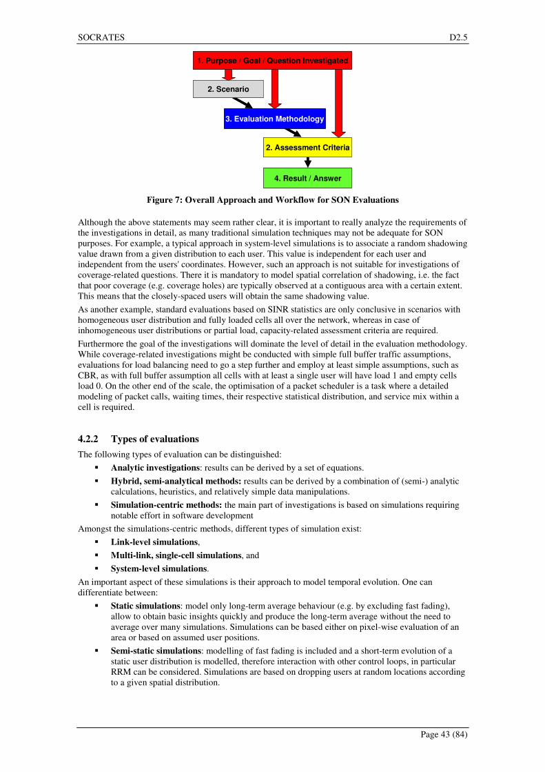
SOCRATES D2.5

(84)

1. Purpose / Goal / Question Investigated

2. Scenario

3. Evaluation Methodology

2. Assessment Criteria

4. Result / Answer

1. Purpose / Goal / Question Investigated

2. Scenario

3. Evaluation Methodology

2. Assessment Criteria

4. Result / Answer

Figure 7: Overall Approach and Workflow for SON Evaluations

Although the above statements may seem rather clear, it is important to really analyze the requirements of

the investigations in detail, as many traditional simulation techniques may not be adequate for SON

purposes. For example, a typical approach in system-level simulations is to associate a random shadowing

value drawn from a given distribution to each user. This value is independent for each user and

independent from the users' coordinates. However, such an approach is not suitable for investigations of

coverage-related questions. There it is mandatory to model spatial correlation of shadowing, i.e. the fact

that poor coverage (e.g. coverage holes) are typically observed at a contiguous area with a certain extent.

This means that the closely-spaced users will obtain the same shadowing value.

As another example, standard evaluations based on SINR statistics are only conclusive in scenarios with

homogeneous user distribution and fully loaded cells all over the network, whereas in case of

inhomogeneous user distributions or partial load, capacity-related assessment criteria are required.

Furthermore the goal of the investigations will dominate the level of detail in the evaluation methodology.

While coverage-related investigations might be conducted with simple full buffer traffic assumptions,

evaluations for load balancing need to go a step further and employ at least simple assumptions, such as

CBR, as with full buffer assumption all cells with at least a single user will have load 1 and empty cells

load 0. On the other end of the scale, the optimisation of a packet scheduler is a task where a detailed

modeling of packet calls, waiting times, their respective statistical distribution, and service mix within a

cell is required.

4.2.2 Types of evaluations

The following types of evaluation can be distinguished:

� Analytic investigations: results can be derived by a set of equations.

� Hybrid, semi-analytical methods: results can be derived by a combination of (semi-) analytic

calculations, heuristics, and relatively simple data manipulations.

� Simulation-centric methods: the main part of investigations is based on simulations requiring

notable effort in software development

Amongst the simulations-centric methods, different types of simulation exist:

� Link-level simulations,

� Multi-link, single-cell simulations, and

� System-level simulations.

An important aspect of these simulations is their approach to model temporal evolution. One can

differentiate between:

� Static simulations: model only long-term average behaviour (e.g. by excluding fast fading),

allow to obtain basic insights quickly and produce the long-term average without the need to

average over many simulations. Simulations can be based either on pixel-wise evaluation of an

area or based on assumed user positions.

� Semi-static simulations: modelling of fast fading is included and a short-term evolution of a

static user distribution is modelled, therefore interaction with other control loops, in particular

RRM can be considered. Simulations are based on dropping users at random locations according

to a given spatial distribution.

SOCRATES D2.5

(84)

� Dynamic simulations: in addition to fast fading, also dedicated modelling of user mobility and

traffic dynamics is performed. The detailed modelling gives in-depth insight in dynamic

behaviour of the system, however, due to complexity reasons, typically only a few seconds or up

to minutes can be modelled with full level of detail.

The three different approaches to temporal modelling are listed in order of increasing complexity,

simulator implementation effort and runtime requirements, as depicted in Figure 8. The x-axis gives the

elapsed time in a real system that is typically simulated, the y-axis is the complexity and effort for

implementation, testing, and conducting evaluation. The 3rd

dimension shows that each type of simulator

can use either simple homogeneous (e.g. hexagonal grid) scenarios, or inhomogeneous settings for

deployment and parameterisations of network nodes, or even be based on real-world data bases (e.g.

topographical height, clutter (land use) data, building data, traffic data, pathloss maps, etc.).

As many SON algorithms will be based on statistics and react on slow variations in the network, on of the

biggest challenge in SON-related simulations is how to model long real-time periods with an appropriate

trade-off between simulation complexity and accuracy of the results. One possible approach to this

problem is denoted as "SON" in Figure 8, it is based on using a sequence of static snapshots, each

representing a steady state of the system, which has already converged to the changed situation imposed

e.g. by an eNB failure, load change, or change in traffic mix. Apart from the change one wishes to

examine, it is important to keep a consistent modelling of other parameters and processes, i.e. to maintain

identical or consider the correlation in shadowing, user distribution, etc. This will allow to capture the

long-term dynamics between system state and SON algorithm as a series of iterative responses, each

based on converged status. More details on this approach and ways to perform dedicated investigations of

the transient times are given in Section 4.4.

real-time duration of simulation

co

mp

lexit

y a

nd

eff

ort

scen

ario

com

plexi

ty

• basic concept decisions

• long-term average

• maximum gain

STATIC

• impact of short-term

fading and

scheduling

• concept refinement

SEMI-STATIC

+ long-term time steps with consistentmodelling of correlated processes (user distribution, shadowing, etc.)

• iterative response

of system due to SON algorithm

• capturing long-term dynamics

SON

DYNAMIC• mobility aspects

• detailed traffic models

• interaction of SON with other control and

adaptation mechanisms

real-time duration of simulation

co

mp

lexit

y a

nd

eff

ort

scen

ario

com

plexi

ty



• maximum gain

STATIC



• maximum gain

STATIC


fading and

scheduling


SEMI-STATIC


fading and

scheduling


SEMI-STATIC


fading and

scheduling


SEMI-STATIC

+ long-term time steps with consistentmodelling of correlated processes (user distribution, shadowing, etc.)




SON




SON









• mobility aspects




Figure 8: Complexity and Simulated Real-Time Duration of System-Level Simulations

4.3 Abstractions and simplifications in modelling

In order to keep evaluations feasible abstractions and simplifications are required in modelling. This

section reviews the particularities of SON-related investigations and discusses general guidelines to arrive

at such simplifications. A high-level overview of useful abstraction levels for the use cases addressed in

SOCRATES D2.5

(84)

SOCRATES is given, while any kind of more detailed discussion of use-case specific modelling issues

will be provided in documents with dedicated focus on the individual use case.

4.3.1 SON simulation challenges

System-level simulations are usually either targeted towards system design or network planning. For

system design it is important to capture relevant aspects of typical deployments and avoid designing for a

single particular case. Furthermore many simulation campaigns are required until system design is

finished, i.e. the complexity of the investigations needs to be limited. In case of open standards, such as

LTE, need to be acceptable by the whole community contributing to standardisation. Therefore

simulations for system design are typically based on generic and homogeneous scenarios with limited

complexity and requirements for additional input data (such as costly data bases). The well-known

hexagonal grid deployment is one example of a widely-accepted scenario for system design and

performance studies.

Network planning, on the other hand, doesn't intend to improve the system as such but wants to improve

the deployment of a system in a particular region, i.e. ensure sufficient coverage and capacity. Therefore

instead of general conclusions or typical behaviour the scope of the investigations is a specific given

environment with its particular and inhomogeneous combination of terrain, land use, buildings,

infrastructure, distribution of network elements, user traffic distribution, etc. Therefore coverage and

capacity calculations are typically based on complex and expensive data bases that serve as input to the

simulator.

A particular challenge of SON simulations is that it falls in between both categories, as it is

predominantly a system design task, but partly tries to replace network planning tasks (or deficiencies) by

automatic algorithms. Furthermore SON typically reacts on inhomogenities typically neglected by

traditional system design studies, such as unequal user distribution in time and space.

As mentioned earlier, also the need to capture long real-time periods within simulations is a challenge,

even more since the SON algorithm needs to work properly considering all other existing adaptation

mechanisms in LTE, which work on multiple time scales already (cf. link adaptation, RRM, etc.).

To address these challenges, SON simulations need to be designed in a strictly question-driven mode

(What is the main question? What do I need to model to which level of detail? What is most likely

irrelevant?) and combine relevant characteristics of traditional system-level simulations for system studies

and for network planning.

4.3.2 General guidelines to derive abstractions and simplifications in modelling

The abstraction and simplification level of the system needs to be defined on a use case basis and is

beyond the scope of this document. However, a high-level overview of general guidelines is given.

Basic needs on the simulations include:

• To capture the variation of the quantity the SON algorithm will react upon. Relevant variations

for SON are

� propagation/mobility effects: fast fading, shadowing,

� usage effects: load, traffic mix,

� change in NW topology: eNB insertion/deletion, cell outage,

� changes in environment (construction, seasonal effects).

• To capture mechanisms that change the statistics of the quantity the SON algorithm will react

upon in case the resulting statistic is not known.

• To capture other adaptation mechanisms with similar time scales in order to ensure system

stability

• To capture other adaptation mechanisms that address the same effect in order to evaluate only

additional gain provided by SON (e.g. in order to evaluate inter-cell interference coordination

by SON, on needs to model all other functions managing interference in the system, such as the

scheduler, MIMO, interference cancellation techniques at Tx and Rx)

SOCRATES D2.5

(84)

It needs also to be emphasised that SON system design should be based on typical and "average"

assumptions (note that "average" can also mean "typical worst-case" in this context). While it may be

tempting to use more and more detail in modelling assumption, on needs to make sure that for every such

detailed assumption (e.g. assuming a dedicated traffic mix) an statistical averaging effect (e.g. Monte

Carlo / statistical evaluation of individual simulation campaigns using different traffic mixes) is required

to obtain the typical behaviour. Having multiple such Monte Carlo components will easily require

infeasible simulation effort until reliable statistics can be obtained. In addition, the risk to do system

design to some particular assumption increases. As a general guideline, it is desirable to have just enough

level of detail than required for deriving the required conclusions.

Figure 9 gives an overview of the envisaged level of detail in modelling propagation channel, data traffic,

mobility, different layers, interfaces, downlink, uplink, and different network nodes for the different use

cases addressed in SOCRATES. The following abbreviations are used:

• COM: cell outage management

• CHM: coverage hole management

• LB: load balancing

• HO: handover

• PS: packet scheduling

• AC/CC: admission control / congestion control

• HeNB HO: Home eNB handover

• HeNB ICO: Home eNB interference coordination

• ICO: interference coordination

• MRR: management of relays and repeaters

Obviously the table can only give a high-level and simplified overview on the requirements. For further

detail, the reader is referred to the detailed discussion of the use cases, e.g. the use case profiles and

simulation tool requirements discussed in Chapter 4 of [2].

The colours in Figure 9 indicate that no modelling is required at all (green colour), simplified models are

required (yellow colour), or detailed modelling is necessary (red colour).

Detailed channel and traffic models are required for HO, PS, AC/CC, and HeNB HO, i.e. for all SON use

cases related to mobility or RRM functionality. Apart from AC/CC, also detailed mobility models are

required. For interference aspects of HeNBs static simulations are considered sufficient. Other use cases

may use simplified models, e.g. averaging already over short-term fading effects, or using semi-static or

static simulations. The latter are considered sufficient for interference aspects of HeNBs.

Considering functionality in different layers of the protocol stack, protocols over different interfaces, and

modelling of different NW nodes, we can differentiate between not modelled at all (green), modelled

based on simple models (e.g. simple correction factors, or probabilistic modelling of associated errors and

delay, yellow) or detailed modelling of functions, protocols, and measurements (red).

In general PHY and MAC layer are most important for the modelling, but also some aspects of RRC need

to be considered at least in simplified ways for LB, HO, PS, AC/CC, and HeNB HO.

PS as well as AC/CC are mainly considered as localized function in the scope of SOCRATES, therefore

S1, X2, and management interfaces are not required to be modelled. As for most SON use cases, both

centralised and de-centralised architectures are under study, typically X2 and management interfaces need

to be modelled with varying degree of detail.

Modelling of UEs and eNBs is required for all use cases. Special requirements. for modelling

functionality, eNB deployment, or user distribution are encountered in LB, HO, PS, and AC/CC .

Therefore the overall classification is yellow. Involvement of MME/SGW in SON functionality is only

foreseen in the HeNB case, otherwise this network nodes can be neglected. Apart from HO, PS, AC/CC,

and ICO OAM needs to be modelled at least in a simplified form, as centralised solutions are within the

scope of investigations.

In general all use cases need to consider both link directions, however, for some use cases, such as PS and

AC/CC work will focus on downlink.

SOCRATES D2.5

(84)

UE

Nod

es eNB

MME/SGW

OAM

ICOHeNB HO HeNB ICOCOM CHM LB HO PS AC/CC MRR

Channel

Traffic

Mobility

La

yer

PHY

MAC

RLC

RRC

PDPC

Inte

rfaces

S1

X2

Mgmt IF

Dire

ct.

Downlink

Uplink

UE

Nod

es eNB

MME/SGW

OAM

ICOHeNB HO HeNB ICOCOM CHM LB HO PS AC/CC MRR

Channel

Traffic

Mobility

La

yer

PHY

MAC

RLC

RRC

PDPC

Inte

rfaces

S1

X2

Mgmt IF

Dire

ct.

Downlink

Uplink

Figure 9: High-level overview on need for modelling details of the individual use cases (green: no

need to model, yellow: simplified model (e.g. simple error / delay model, correction factor, mapping

function, red: detailed model requiring notable dedicated software development)

4.4 Simulation based evaluation methodology

4.4.1 System states and self-optimised algorithm evaluation

The self-optimised algorithm will be triggered as reaction to changes in the system. To evaluate the

algorithm we will have to describe what these changes are. For this purpose, we first introduce the term

system state. The system state describes the status/evolution of the system during a certain time interval

and it consists of the deployment state, traffic state, and radio propagation state. Note here that the self-

optimisation algorithms may directly respond to observed changes in the system performance, which is a

consequence of the single or combined change of the deployment, traffic or radio propagation states.

The system state may be static or dynamic. A static system state is characterized by a static deployment,

traffic/performance and radio propagation states, whereas in a dynamic system state either one or more of

the deployment, traffic, or the radio propagation states are dynamic. In the following paragraph we further

explain these terms with some examples.

� In a static system state:

– The deployment is static. For example, no new nodes are added or removed and no

outages occur.

– The traffic state is static because the traffic’s statistical properties do not vary (e.g.

constant call arrival rate and service mix), the users’ spatial distribution does not change

and the users’ mobility does not change.

– The radio propagation state is static. In this case the statistics of the distance-based path

loss, the shadowing and the multi-path fading are constant.

� In a dynamic system state:

– the deployment might change (e.g. new nodes or outages)

– the traffic state might change i.e. the call arrival rate and the service mix change, the

user spatial distribution changes or the user mobility changes.

– the radio propagation state might change i.e. the statistics of the distance-dependent

path-loss, the shadowing, the multi-path fading change.

SOCRATES D2.5

(84)

4.4.2 Evaluation of SON algorithm in static system state

Consider two static system states A and B as shown in Figure 10. For example these can be two different

traffic states, characterized by different call arrival rates and/or traffic mix. As the system is in static state

(A or B) and -- if we look on longer time scale (e.g. hours/days) -- the statistical properties of the system

are constant (i.e. constant arrival rate and/or traffic mix). If we look on shorter time scales (e.g. seconds to

minutes) there are ‘local variations’ around the static system state for example the number of currently

active users per traffic class (e.g., voice, data, video, etc). These local variations are also shown in Figure

10.

Time

Local variationsStatistical

realisations

State A

State B

Time

Local variationsStatistical

realisations

State A

State B

Figure 10: “Static”system states.

The SON evaluations in the static system state conditions are valuable for two reasons:

1) The SON algorithm might be triggered as reaction to a system change from state A to state

B. Therefore, it is necessary to test the algorithm behaviour (e.g., performance and

convergence) given the static system state A (or B) while the starting network parameter

configuration are from the other system state B (or A).

2) It is important to check whether the SON algorithm might also be triggered by changes in

the system state at a smaller time scale illustrated with the local variations in Figure 10.

Furthermore, if the SON algorithm is triggered by these local variations it is important to

evaluate what is the scale of local variations that trigger the algorithm and how is that

affecting the network performance.

As example consider the packet scheduling use case and a change in the service mix. Such change may

trigger the SON algorithm, which will derive new scheduler parameters. Consider now a constant service

mix. At a shorter time scale (from seconds to minutes) the relative number of simultaneous calls in the

system is not constant. In this sense, the SON algorithm that optimises the scheduling parameters might

or might not ignore the variations in the system state at this time scale. With these evaluations it can be

assessed what is the desired time scale of operation for the SON algorithm and also what kind of input

sensitivity is desired (i.e. whether or not to ignore the ‘local variations’). An additional, interesting

question is how fast the SON algorithm converges to the optimal parameter settings if it is put to work

into a static system state with a suboptimal set of parameters as starting point.

It should be studied per use case how the SON algorithm should react (triggered or not triggered) to

different type of variations in the system state. The assessment methodology should allow the evaluation

of the performance of the SON algorithm in all for the use case relevant system changes.

4.4.3 Evaluation of SON algorithm in dynamic system state

Consider a system which evolves between state A and state B as shown in Figure 11. The duration of a

system state change varies and can range from:

a) Rapid state change that can be either instantaneous (e.g. due to the insertion of a new node

or a cell outage) or take few seconds or minutes (e.g. due to a large accident or busy hour).

System State

SOCRATES D2.5

(84)

b) Slow state change that takes place over a longer period, e.g. several hours, weeks, months or

even years (e.g. due to seasonal effects, the introduction of a new service or user population

migrations).

System State

Time

Rapid system state

change

Slow system state

change

Tsystem_change Tsystem_change

State A

State B

Figure 11: System state changes.

The question is how to evaluate the performance of the SON algorithm in rapid and slow system state

changes, having in mind that simulating the whole system state change will be in many cases unfeasible

to due constraints in simulation time and/or computation power.

4.4.4 Examples of simulation-based SON evaluation methodology

In this section we assume a simulation-based evaluation approach. We explain with three examples

applied to three (sub-)use cases a possible evaluation methodology for the developed self-optimisation

algorithms.

4.4.4.1 Evaluation of a Cell Outage Compensation (COC) algorithm

In this example, we consider a cell outage compensation algorithm. We consider three system states:

� State A: pre-outage situation

� State B: post-outage situation without COC

� State C: post-outage situation with COC

Figure 12 illustrates the system performance in terms of supported traffic. The red arrow shows the time

instant at which the system change, the cell outage, occurs. The letters on the curves refer to the states A,

B or C.

The evaluation of the COC algorithm consists of three steps:

� STEP 0- Sensitivity analysis (via static or dynamic simulations) i.e. given state B check

which parameters adjustments have the highest impact on the system performance.

� STEP 1-Self-optimisation algorithm design (via static or dynamic simulations). Design the

self-optimisation algorithm. Given state B and starting from the parameter settings in state A

perform step-wise adjustments of the parameters identified in STEP 0. After each COC step

measure the performance. For the following steps use the parameters from the previous step.

How optimal is the resulting performance? What is the convergence time of the algorithm?

� STEP 2-SON Implementation (via dynamic simulations) i.e. given the state change from state

A to state B and given the algorithm developed in STEP 1 perform dynamic simulations.

Consider practical constraints like: available measurements, how long can/should we measure

and how accurate are (should) the measurements (be). Check the resulting system performance.

SOCRATES D2.5

(84)

time

Su

pp

ort

ed

tra

ffic

A

B

C

Outage

Figure 12: The system states before and after a cell outage event.

4.4.4.2 Evaluation of the self-optimised packet scheduler

In this example, we consider the packet scheduling optimisation use case. We assume a packet scheduler

with parameters α and ξ. The self-optimisation algorithm aims at finding the optimal settings of these

parameters based on the system conditions. In this example we assume that it reacts on significant

changes in the service mix. We consider three system states:

� State A: state with the old service mix

� State B: introduction of the new service i.e. a new service mix, without self-optimisation

algorithm

� State C: introduction of new service i.e. a new service mix, with self-optimisation algorithm

Figure 13 shows the system performance in terms of packet loss. The red arrow shows the instant at

which the new service mix is introduced. The letters on the curves refer to the states A, B or C.

The evaluation of the self-optimised packet scheduling algorithm consists of three steps:

� STEP 0 Sensitivity analysis (via static or dynamic simulations). Given the traffic mix in state

A and state B optimise αA, ξA and αB, ξB. Determine sensitivity of optimal α and ξ w.r.t to

service mix.

� STEP 1 SON Design (via static or dynamic simulations). Design a self-optimised algorithm.

Starting from αA, ξA and given the traffic mix in state B perform step-wise adjustments of the

scheduling parameters α and ξ. After each step measure the performance. Observe the

convergence to αB, ξB. What is the convergence time? How close gets the solution of the self-

optimised algorithm to the optimal performance?

� STEP 2 SON Implementation (via dynamic simulations) i.e. given the state change from state


Consider practical constraints like: available measurements, how long we can measure and how

accurate the measurements are. Check the resulting system performance.

time

Pack

et

los

s

A

B

C

introduction

new service

time

Pack

et

los

s

A

B

C

introduction

new service

Figure 13: Packet loss before and after a service mix change for a system with and without

scheduler self-optimisation.

SOCRATES D2.5

(84)

4.4.4.3 Evaluation of the self-optimised algorithm for handover optimisation

In this example, we consider the handover optimisation use case, see [1] Section 3.3.1. The handover

algorithm is based on signal strength measurements (e.g., RSRP measurement) from the serving and

neighbouring cells, see TS 36.331. This example assumes that the most relevant parameters for handover

optimisation are the time interval α where the signal strength is below a predefined threshold, and the

signal strength (RSRP) handover threshold ξ. It is also assumed that the self-optimisation algorithm reacts

on significant changes in the average user speed. We consider three system states:

� State A: system state with the old average user speed

� State B: increase in average user speed, without SON algorithm

� State C: increase in average user speed, with SON algorithm

The evolution of the system performance in terms of handover success ratio is illustrated in Figure 14.

The red arrow marks the moment at which the increase of the user speed starts. The letters A, B and C

refer to the system state A, B or C.

The evaluation methodology of the self-optimised algorithm consists of these three steps:

� STEP 0-Sensitivity analysis (via static or dynamic simulations). Given the average speed in

state A and state B optimise αA, ξA and αB, ξB, respectively.

� STEP 1 SON Design (via static or dynamic simulations). Design the self-optimisation

algorithm. Starting from αA, ξA and given the average speed in state B perform step-wise

adjustments of the speed. Does the algorithm converge to αB, ξB ? How fast does it converge?

how close does the solution obtained get to αB, ξB ? After each step measure the system

performance.

� STEP 2 SON Implementation (via dynamic simulations) i.e. given the state change from state


Consider practical constraints: how long can be measured and how accurate are the

measurements. Check the performance of the self-optimised algorithm.

Figure 14: HO success ratio before and after increase in user speed for a system with and without

handover self-optimisation.

4.4.5 Generalised approach for simulation-based SON evaluation

The evaluation methodology presented in the examples of the previous section can be generalised in the

following way. Consider three states as illustrated in Figure 15:

� State A: the initial state, before the change. We assume optimal parameters are in place.

� State B: change in the system state, without SON algorithm

� State C: change in the system state, with SON algorithm

The evaluation methodology consists of three steps:

� STEP 0 Sensitivity analysis (via static or dynamic simulations)

– What should trigger SON and at what significant change? What are the most relevant

configuration parameters that have to be adjusted?

� STEP 1 SON Design (via static or dynamic simulations)

– Design the adjustment logic for the identified parameters in STEP 0 and check

convergence and performance optimality

time

HO

su

ccess r

ati

o increase in user speed

AB

C

SOCRATES D2.5

(84)

� STEP 2 SON Implementation (via dynamic simulations)

– Check SON performance with changing system state with practical constrains about

how long and how accurate we can measure.

Figure 15: System performance before and after a system change for situations with and without

SON functionality.

Although in this stage of the project it is still unclear whether the proposed 3-STEP methodology is

suitable for each SON use case, we presume that the underlying general principles are widely acceptable.

Besides it should be determined on a case by case basis whether static or dynamic simulations can be

performed at step 0 and step 1.

4.5 Benchmarking as an assessment approach

If the previous sections are targeted to the assessment of a single self-organising algorithm, this section

gives guidelines to do a mutual comparison of different self-organisation methods developed for a given

use case, and moreover to compare their achieved performance, capacity, cost, revenue, to the case with

manual network operation.

In this section, we describe several approaches for such benchmarking. They are primarily outlined from

the perspective of a self-optimisation use case, while at the end some comments are made regarding self-

configuration and self-healing use cases.

Starting point is a specific scenario in terms of e.g., the propagation environment, service mix, traffic

characteristics, spatial traffic distribution. For such a scenario, the achievements of the different

developed self-optimisation algorithms comprise measures of e.g., performance, complexity and CAPEX,

and are further characterised by the number of parameter adjustments that are made per time unit which is

a key contributor to the OPEX (see Section 3.1.6).

The example Figure 16 below visualises fluctuations in the traffic / mobility / propagation characteristics,

and the algorithm-specific timing of induced radio parameter adjustments.

tra

ffic

/mo

bil

ity/p

rop

ag

ati

on

ch

ara

cte

ris

tic

s

time

Parameter adjust-ment instants for

self-optimisation

algorithms A, B, …

tra

ffic

/mo

bil

ity/p

rop

ag

ati

on

ch

ara

cte

ris

tic

s

time

Parameter adjust-ment instants for

self-optimisation

algorithms A, B, …

Figure 16: Fluctuations in traffic / mobility / propagation characteristics, and the algorithm-specific

timing of induced radio parameter adjustments.

In Figure 17, example values of the performance indicators obtained at the end of the simulations are

shown. Observe that e.g., self-optimisation algorithm SOA achieves the highest performance, which can

be exploited to achieve the lowest CAPEX, but in order to achieve this it requires a lot of measurements

time

Sys

tem

Perf

orm

an

ce A

Bchange in system

C

SOCRATES D2.5

(84)

(~ complexity) and parameter adjustments per time unit (~ OPEX in case of manual optimisation; it is

noted that the ‘OPEX’ bar in the figure indicates the associated OPEX in the ‘manual’ equivalent of the

self-optimisation algorithm, i.e., the ‘saved OPEX’). In contrast, algorithm SOD is significantly less

complex but consequently achieves worse performance and CAPEX.

SOA

Go

S/Q

oS

CO

MP

LE

XIT

Y

OP

EX

CA

PE

X

Go

S/Q

oS

CO

MP

LE

XIT

Y

OP

EX

CA

PE

X

SOB

Go

S/Q

oS

CO

MP

LE

XIT

Y

OP

EX

CA

PE

X

SOC

Go

S/Q

oS

CO

MP

LE

XIT

Y

OP

EX

CA

PE

X

SODSOA

Go

S/Q

oS

CO

MP

LE

XIT

Y

OP

EX

CA

PE

X

SOA

Go

S/Q

oS

CO

MP

LE

XIT

Y

OP

EX

CA

PE

XGo

S/Q

oS

CO

MP

LE

XIT

Y

OP

EX

CA

PE

X

Go

S/Q

oS

CO

MP

LE

XIT

Y

OP

EX

CA

PE

X

SOB

Go

S/Q

oS

CO

MP

LE

XIT

Y

OP

EX

CA

PE

X

Go

S/Q

oS

CO

MP

LE

XIT

Y

OP

EX

CA

PE

X

CO

MP

LE

XIT

Y

OP

EX

CA

PE

X

SOB

Go

S/Q

oS

CO

MP

LE

XIT

Y

OP

EX

CA

PE

X

SOC

Go

S/Q

oS

CO

MP

LE

XIT

Y

OP

EX

CA

PE

X

Go

S/Q

oS

CO

MP

LE

XIT

Y

OP

EX

CA

PE

X

SOC

Go

S/Q

oS

CO

MP

LE

XIT

Y

OP

EX

CA

PE

X

SOD

Go

S/Q

oS

CO

MP

LE

XIT

Y

OP

EX

CA

PE

X

Go

S/Q

oS

CO

MP

LE

XIT

Y

OP

EX

CA

PE

X

SOD

Figure 17: Example values of obtained performance indicators.

In general, it is hard to compare SOA through SOD given the conflicting performance objectives, e.g., SOA

outperforms SOD in terms of CAPEX, but SOD outperforms SOA in terms of complexity. One approach to

enforce a strict overall ranking is to weigh/combine the different measures into some utility function and

rank the algorithms based on the obtained utility values. In the following paragraph, an example of this

approach extracted from the home eNodeB use case is presented.

Consider algorithm X (Alg_X) a SON algorithm for the home eNodeB optimisation use case. The overall

metric for the assessment of Alg_X is the weighted sum of the gains from the SON algorithm X relative to

the reference (ref) case when no SON algorithm or a very basic SON algorithm is deployed. Those

metrics are the A reference case is required to enable normalisation of the different metrics. Potentially,

different reference cases will be required for different scenarios. Expressed in an equation, this results in:

refcapacity

XASONcapacity

refcoverage

XASONcoverage

SON_Alg_XSON_Alg_XXA

M

M

M

M

scoreQoS scoreGoSM

_

lg___

_

lg___

lg_

δχ

βα

++

⋅+⋅=

Where GoS score and QoS score are the weighted sum of some QoS and some blocking/dropping metris,

respectively and Mcoverage and Mcapacity are some coverage and capacity metrics. The weighting factors α, β,

γ and δ reflect the relative importance of different metrics. For example, if the GoS score is twice as

important as the QoS score, then α will be twice as large as β. Weighting factors can also be 0, if the

metric is considered not relevant for a certain scenario. The absolute value of MAlg_X has no meaning.

However, the relative values of the overall metric will be used to compare different solutions. For all

metrics, higher values correspond with better performance.

Another approach is to select one measure as single target measure, place constraints on the other

measures and rank only those algorithms that meet the constraints on the other measures based on the

target measure.

Whereas the above discussion outlines an approach to compare different self-optimisation algorithms, a

more difficult challenge is to compare a self-optimisation algorithm with a case of manual optimisation.

For such a comparison one needs to specify the manual optimisation method, in order to derive estimates

for the different performance, capacity, etc., measures.

In an extreme case, we could assume that a ‘manual operator’ freezes its radio parameters once and for

all. In that case it would make sense to do an off-line optimisation of the parameter set such that the

overall performance is optimised, considering the given scenario with varying traffic, mobility and

propagation characteristics. For this scenario, the performance indicators of the manual operated

algorithm obtained with the optimised set of parameters are compared with the performance indicators of

the self-optimised algorithm.

In practice, however, a network operator will monitor such characteristics as well as the achieved

performance level, and occasionally redetermine the radio parameters. Depending on the operator’s

policy this may happen more or less frequently: a quality-oriented operator is likely to do more frequent

adjustments than a cost-oriented operator. In order to model this in a reasonable way, we propose to

define ‘manual optimisation algorithms’ MOA through MOD (continuing the above example) such that

SOCRATES D2.5

(84)

they manually adjust radio parameters at the same time and to the same values2 as the corresponding self-

optimisation algorithms with the same label. An example comparison of SOA with MOD is visualised in

Figure 18, concentrating on (for example) CAPEX and OPEX-related measures.

SOA

OP

EX

CA

PE

X

OP

EX

CA

PE

X

MOD

self-optimisation manual optimisation(benchmark)

assess e.g. OPEX/CAPEX gainsof SOA with regard to benchmark MOD

OPEX gain

CAPEX gain

SOA

OP

EX

CA

PE

X

OP

EX

CA

PE

X

MOD

self-optimisation manual optimisation(benchmark)

assess e.g. OPEX/CAPEX gainsof SOA with regard to benchmark MOD

OPEX gain

CAPEX gain

Figure 18: Comparison of SOA with regard to benchmark MOD.

Assuming that self-optimisation reduces OPEX to zero3, the OPEX gain achieved by self-optimisation is

indicated by the height of the OPEX bar associated with the MOD algorithm. In order to convert this

measure to a monetary value, one needs to assume some amount of effort involved in a radio parameter

adjustment, which may be estimated by a network operator. In this light, we also note that it may be wise

to distinguish between different types of parameter adjustments that involve different degrees of manual

effort. The CAPEX gain is trivially indicated by the difference in the algorithms’ CAPEX values.

Following this approach for different combinations of SOX and MOY we could generate tables such as

Table 3, where the ‘+’, ‘-‘ and ‘0’s are just qualitative indicators; actual numerical values should be

determined via the simulation studies. Observe that introducing self-optimisation in the network of

quality-oriented operator is likely to establish the highest OPEX gains, but the lowest CAPEX gains.

0++++++MOD

-0+++MOC

---0+MOB

------0MOA

SODSOCSOBSOA

0++++++MOD

-0+++MOC

---0+MOB

------0MOA

SODSOCSOBSOA

+

++

+++

++++

SODSOCSOBSOA

+

++

+++

++++

SODSOCSOBSOA

CAPEX GAINS OPEX GAINS

quality

orientedoperator

costoriented

operator

Table 3: Qualitative indicators for CAPEX and OPEX gains when introducing self-optimisation.

Another more simplistic approach could compare the We finalise this subsection with some comments

about benchmarking for self-configuration and self-healing use cases, noting again that the above

approach was primarily outlined from the perspective of self-optimisation use cases.

Regarding self-configuration, the OPEX gain can be estimated by consulting one or several network

operators what human effort is required for the different subtasks that are involved. See also related

comments in Section 3.1.6. Depending on the set of subtasks that is automated by self-configuration

methods, the OPEX gain can be determined. We expect that no significant CAPEX gains are achieved

from self-configuration. In terms of performance and revenue, there may be a gain due to improved

GoS/QoS and correspondingly, possible increased revenue. This is however less likely if the deployment

of new sites or features is done at night, which is typically the case.

Regarding self-healing, including cell outage compensation, there may be some OPEX gain if the cell

outage detection mechanism speeds up the problem identification and if the cell outage compensation is

2 The assumption that the manual optimisation algorithm makes the same adjustments at the same time is easily

relaxed in an actual quantitative study, e.g., by introducing randomised discrepancies in the (timing of) parameter

adjustments.

3 This assumption may need to be relaxed somewhat, since even self-optimised networks will require some human

involvement in terms of performance monitoring, sanity checking, etc. In any case, for the purpose of explaining

the approach this assumption is acceptable.

SOCRATES D2.5

(84)

automated, which would otherwise be done manually. Still, most OPEX is related to actually fixing the

failed site, which will remain even with self-healing. The impact of self-healing on the GoS/QoS and the

associated revenues was already discussed in Section 0. In terms of CAPEX gain, we can see this

originate from a need for less redundancy to cope with potential failures (in a typical network, however,

such redundancy is not used in the radio interface) or potentially even from a reduced requirement on

eNB reliability, although this may not the recommended way to exploit the gains from self-healing.

SOCRATES D2.5

(84)

5 Reference scenarios

5.1 Introduction

This section summarises the current status of the development of the realistic SOCRATES reference

scenarios. It replaces section 3.2.2 in D2.3 [3]. The work has been split into two main parts: the

development of data formats (Section 5.2) and the generation of the data for the realistic reference

scenarios (Section 5.3).

The work is carried out in 4 intermediate steps that are processed consecutively:

Activity 1: Basic macro scenario

First a basic scenario is being generated based on input from an operator. It consists of a macro cell layer.

Realistic traffic and mobility data is being generated for this layer. The result comprises a complete

scenario, which fulfils the requirements of most use case studies.

Activity 2: Addition of Femto- and Pico-Cells

In a second step, an indoor cell layer is added to the scenario. For the indoor layer no detailed real-world

input is available, such that this data has to be generated artificially. Key challenges are the realistic

distribution of cells, traffic, and the generation of pathloss data (in particular outdoor to indoor, and

indoor to outdoor pathloss maps).

Activity 3: Addition of the time aspect:

Many use cases require the inclusion of a time aspect into the reference scenarios. This in particular

includes mid- and long-term traffic changes in the traffic and mobility patterns as well as changes of the

network layout, e.g., equipment failures, addition of new sites. Appropriate scenarios will have to be

developed.

Activity 4: Scenario add-ons

In a last step aspects are added to the scenario data, that are considered to be least important (e.g., relays

and repeaters), or for the modelling of which not sufficient information were available at the project start

(e.g., MIMO).

5.2 Data Formats

In the EU funded project MOMENTUM significant effort has been spent on the definition of a UMTS

scenario format [31][34]. This format has later been improved and extended in the COST 293 sub-activity

“MORANS” [36]. The UMTS specific MOMENTUM and MORANS data formats are specified in XML

and extensively described in [31][32][33]. The according schemas can be accessed from the

MOMENTUM homepage [35].

The SOCRATES consortium has decided to use the MORANS data format as a basis for an extended data

format that is going to be developed within SOCRATES.

In Figure 19 the basic structure of the XML data is presented. The main scenario file is “Anchor.xml”. It

contains references to all data contained in the scenario.

The remainder of this chapter will describe the necessary extensions in more detail.

SOCRATES D2.5

(84)

Figure 19: Basic Structure of the MORANS Data Format

5.2.1 Hardware requirements

Since the MORANS data formats are UMTS specific and SOCRATES focuses on the LTE system it is

necessary to add the new hardware available for LTE to the SOCRATES data formats. It is planned to

add home eNodeBs, relays, repeater and multi-antenna arrays for MIMO and beam forming.

Additional extensions are necessary due to the fact that the highest network entity in the MORANS data

formats is the NodeB. The SON functions developed in the SOCRATES project will be implemented

locally, distributed or centralised. Information exchange between eNodeBs and other eNodeBs or MMEs

is needed to allow this. Figure 20 shows the interfaces between the eNodeBs and MMEs. The data

formats need to provide the information about the interconnection of the network elements.

SOCRATES D2.5

(84)

Figure 20: LTE network topology

5.2.2 Multi-Layer data

The introduction of home eNodeBs to the LTE network entails the need for multi-layer information in the

data formats. The impact of a home eNodeB to the surrounding area depends on the location of the home

eNodeB. To study the effect of a home eNodeB in indoor, indoor-to-outdoor or outdoor-to-indoor

scenarios the propagation maps have to be available for every building-level. The data formats have to be

extended accordingly

5.2.3 Multi-Resolution data

The needed simulation accuracies for the algorithm development in the different use cases vary dependent

on the impacted network area and individual evaluation objective. To provide the network data only in

one (the highest) accuracy will slow down the simulations with lower simulation accuracy needs. The

SOCRATES data formats will provide the network data in several accuracies as indicated by the two

grids in Figure 21. At the actual stage it is planned to have two resolutions (10m and 100m).

Figure 21: Multi-Resolution data

5.2.4 Network condition changes

The SON functions developed in every SOCRATES use case influence several control parameter settings.

Some control parameter changes, e.g. antenna tilt, antenna azimuth, lead to new network conditions that

have to be available in the network data. The changed signal propagation is one example for this kind of

data.

Additional scenario data is needed for the algorithm development and evaluation in some use cases. Cell

outages or coverage holes have to emerge in the simulations for these use cases. This information has to

be available in the network data. Other important simulation scenarios are high user concentrations,

groups of high speed users or home eNodeBs that are switched “on” and “off”.

SOCRATES D2.5

(84)

5.3 Scenario Data

For the realistic reference scenarios two areas have been selected; the first scenario is a city and

surrounding countryside, including hilly terrain, and the second scenario is a dense urban area. For each

of the areas, a realistic LTE network is generated based on real network input on the existing 2G and 3G

networks in the areas.

The remainder of this chapter is dedicated to activity 1 (cf., Chapter 5.1), which is being processed in

March 2009.

5.3.1 Network configuration

For the first scenario an area of 72 km x 37 km has been chosen (cf., Figure 22). For the area, site data has

been provided for 199 sites (97 GSM only, 102 UMTS or co-located).

For the artificial LTE network, the same layout as for UMTS is assumed. This in particular includes the

same locations, sector orientation, antenna tilt. The resulting network comprising 102 sites and 306 cells

is depicted in Figure 23. The additional GSM sites will be considered as potential site candidates for, e.g.,

the coverage hole management (CHM) use case.

Figure 22: First scenario area

SOCRATES D2.5

(84)

Figure 23: LTE network based on a real UMTS network layout (red marks: GSM site locations)

5.3.2 Pathloss data

For all antenna locations an operator has provided realistic pathloss prediction grids for the 2.6 GHz band.

As described in section 5.2.3, the predictions employ two levels of resolution. For the 3km x 3km area

close to the base station, high resolution prediction data with a pixel size of 10m is available. For the rest

of the scenario the data is available with 100m pixel size.

The availability of two levels of resolution poses the question which resolution to use (where). The usage

of 100m pixel data throughout the scenario can be expected to be too unrealistic, because important

effects might not be captured. On the other hand the consideration of a pixel size of 10m throughout the

scenario results in a number of pixels (26.64 million) which might be too large for most simulators used

in the project. It is thus proposed to consider multi-resolution data. That is, to use a resolution of 10 m in

areas where at least one grid with high resolution is available and to use 100m pixel resolution elsewhere

(Figure 24). As a result the number of pixels can be reduced without loss of accuracy to approx. 6.5 or

10.9 depending on if only UMTS site locations or all site locations are considered.

SOCRATES D2.5

(84)

Figure 24: Multi-resolution scenario, pixel sizes: 10m (yellow) and 100m (blue)

5.3.3 Clutter data

Clutter Data (land use information) is not available.

In the short run clutter data has thus been generated based on average site to site distances (cf., Figure

25).

In parallel more detailed land use information are extracted from the freely available information of the

open-street-maps-project (cf., [37] ). The project provides detailed vector data in XML format. Also, a

rendering engine is provided. The tailoring of this machinery to the specific SOCRATES requirements,

however, requires some additional time.

SOCRATES D2.5

(84)

Figure 25: Clutter data generated based on site-to-site distance (green: "rural", yellow: "sub-

urban", light red: "urban", red: "urban")

5.3.4 Height data

The availability of height data is currently under clarification.

5.3.5 Traffic data

Detailed 3G traffic data will be provided by an operator at a later stage. From this data, LTE traffic data

will be extrapolated based on various assumptions (service types, terminal availability, etc.).

At first, traffic maps have been generated based on very simplified assumptions, i.e., first an equal

amount of traffic is spread over the coverage area of each cell. The resulting traffic grid is consecutively

weighted with clutter type specific weights. One resulting traffic map is presented in Figure 26.

SOCRATES D2.5

(84)

Figure 26: Traffic data generated based on coverage plot and weighted according to clutter data

5.3.6 Mobility data

Once the generation of realistic traffic data has been finalised, the generation of mobility data (i.e.,

mobility grids, cf., [3]) can be carried out. It is planned to employ the open-street-map vector data [37] for

the generation of highly detailed and realistic mobility maps.

5.4 Outlook

At the time of writing this document, the data formats for Activity 1 (cf., Chapter 5.1) are about to be

finalised. With respect to the reference scenario data, most data needs be enhanced (in particular: clutter

data, traffic data, and mobility data). This process mainly depends on the availability of data.

Once activity 1 is finished, a complete macro scenario is available, which is ready to use for most of the

simulation studies to be carried out in the first half of the project.

The reference scenarios will be continuously improved by adding incrementally adding more complexity

(Activities 2-4).

SOCRATES D2.5

(84)

6 Architecture supporting SON functionalities

This chapter provides the description of the high-level architecture and scenarios according to the SON

functionality levels described in Chapter 1 and Figure 2 of [4]. These high-level aspects include an

overview of the LTE network and OAM architecture, and presents different solution concepts to how

self-organisation can be implemented in a network. The three main options considered are centralised,

distributed and hybrid.

Though this deliverable sets the framework for the SOCRATES work packages, especially a preference

for a dedicated SON solution concept cannot be stated clearly yet. Since there exist a number of aspects

as selection criteria for the scenarios (cf. Section 6.4), and the outcome may be different for each of the

use cases, this topic requires a more detailed discussion. Therefore, a more detailed analysis will be made

in SOCRATES work packages 3 and 4, with working out the requirements of the single use cases (e.g.

regarding measurements and information exchange) in detail, and choosing the preferred solution

approach.

6.1 OAM architecture

Management Reference Model

Self-organising networks (SON) consists, amongst others, of self-configuration, self-optimisation, and

self-healing. All these topics are strongly related to the classical management of telecommunication

networks, mainly to the topics of configuration management (CM), performance management (PM), and

fault management (FM). Regarding an implementation of SON topics into future networks it is therefore

necessary to understand the functioning of network management as it is implemented in today’s mobile

radio networks. Since SOCRATES concentrates on 3G networks the management approach as it is driven

by 3GPP is explained in the following.

Basically, telecommunications management is based on the Telecommunications Management (TMN)

standard by ITU-T M.3000 series, which separates the management into several logical layers. These

layers are (top-down):

• Business Management: functions related to business aspects, analyzes trends and quality issues,

providing a basis for billing and other financial reports, business strategies

• Service Management: functions for the handling of services in the network: definition,

administration and charging of services; quality of service (QoS) management, user

administration, service generation etc.

• Network Management: functions for distribution of network resources, providing a complete

network view; configuration, control and supervision of the network, failure management

• Element Management: functions for the handling of individual network elements. This includes

alarm management, handling of information, backup, logging, and maintenance of hardware and

software.

3GPP standardisation describes in [27] a reference model for (mobile) telecommunication network

management. The reference model is strongly related to the TMN model described above, and consists of

several levels of management and interfaces between these levels. The levels are (top-down, cf. also

Figure 27):

• Enterprise Systems (ES) level (includes TMN Business and Service management layers)

• Network Manager (NM) level (functionality according to TMN Network Management layer)

different NMs might be required e.g. in case different network technologies are being used

within one network organisation; some network organisations may, however, have only one NM

level implemented but using tooling within that level supporting functionality of network

equipment and DM / EM from different vendors

• Domain Manager (DM) / Element Manager (EM) level – each NE requires an EM for

management purpose, in a minimum setup one EM is responsible for one NE. Usually the EM is

delivered together with the NE by the manufacturer and therefore proprietary. In 3GPP usually

the expression DM is used, since:

• One DM may server several NEs (e.g. several 3G RNCs or several 1000 3G NodeBs)

• A DM may serve the NEs of one manufacturer (manufacturer domain)

• A DM may serve the NEs of a dedicated geographical domain in large networks

SOCRATES D2.5

(84)

• Network Element (NE) level – this level describes the network elements, such as radio base

stations, controllers, gateways, switches, servers etc.

DM and NM level together are described as the Operations System domain that include the network

(technology) and services related level of management, while the ES domain include the business and

customer related level of management. The ES domain is also often described as Operations and Support

System (OSS), but in some descriptions OSS includes also the NM level. Therefore, the Interface 2 as

described below can in some descriptions be directly connected to the OSS.

In the 3G LTE setting different NEs from different manufacturers must be coordinated at all levels of the

mobile network of one network organisation. One network organisation thereby represents the network of

one operator. For example, handover between NEs of different manufacturers have to work as well as

services must be available at similar quality at all NEs of an operator.

On a separate conceptual level from macro eNodeB on NE level, the “Home NEM” for the direct

integration of Home eNodeB exists. This has to be considered separately as the regular Home eNodeB

operation should be separate from the operation of the regular macro infrastructure.

Organization A

Enterprise Systems

NENENENEEMNE

EM

5

4 5

6

DM

Organization B

DM DM

2 2 2

4a 4a

2

1 1 1 1

5a

EM EM EM

33

Opera

tions S

yste

ms

Itf-P2P

2

NM NM

Itf-N

OS

S

Vendor A

Vendor B

Figure 27: Management Reference Model (Source: [27])

The reference model furthermore describes a set of interfaces between the management levels (denoted

by numbers in Figure 27):

• Interface 1: between the NE and the EM of a single network domain (vendor domain) within a

single network organisation – this interface is usually called “Southbound” interface

• Interface 2: between the EM of a single network domain and the NM of a single network

organisation; the description of this interface is covered by standardisation (3GPP SA5), and the

interface is usually called “Northbound” interface, Itf-N

Note: in some cases the EM level can be part of the NE, such that a direct interface exists

between NE and NM – nonetheless, this interface is an Itf-N and therefore standardised

• Interface 3: between NM and Enterprise Systems of a single network organisation

• Interface 4: between the NMs of a single network organisation, which is usually one network

operator

SOCRATES D2.5

(84)

• Interface 4a: between the EM / DM of a single network organisation; this interface is usually

described as Itf-P2P (peer-to-peer); corresponding standardisation activities are currently

stopped

• Interface 5: between Enterprise Systems and NMs of different network organisations (this is

required in case of national roaming between two operators, for example to exchange billing

information)

• Interface 5a: between DMs / EMs of different network organisations (this is required in case of

national roaming between two operators, for example to exchange configuration information and

measurements to enable handovers)

• Interface 6: between NEs

Integration Reference Point (IRP) is an interface concept for adoption of standardised management

interfaces in telecommunication networks. Three types of IPRs are standardised:

• Interface IRPs: definitions for IRP operations and notifications in a network agnostic manner

• Data Definition IRPs: data definitions applicable to specific management aspects to be managed

via reusing available Interface IRPs and being applied to Network Resources IRPs as applicable

• Network Resources IRPs: definitions for the Network Resources to be managed through the Itf-

N (commonly named "Network Resources IRPs")

In the first phase of 3GPP standardisation, a conceptual requirement specification is defined, including

the description of interface aspects and the identification of use cases. In the second phase, a protocol

independent object-oriented model of the interface based on UML is defined. In the third phase, solution

sets for the IRPs are provided, which then describe a technology-dependent syntax, e.g. GDMO/ASN.1,

XML, CORBA, or Web Services.

IRPs standardised in 3GPP may be implemented in interface types 2 to 5. In current 3GPP standardisation

predominantly protocols and information models for interface type 2 (Itf-N) and to a lesser extent,

interface type 1, are specified. Standardisation for interface types 3, 5 and 5a are for further study (FFS).

The specification of interface types 4 and 6 is in principle out of scope of 3GPP standardisation.

However, with the introduction of 3G LTE, a standard interface between eNodeBs has been introduced

(X2 interface, cf. [28]), which is not primarily intended as a management interface. However, regarding

Self Organising Networks (SON), the X2 interface might be used for the exchange of management related

information.

6.2 LTE / SAE network architecture

The evolution from 3G networks to LTE / SAE brought a substantial change in the network architecture

and the logical interfaces of radio and core network. Whilst in 3G, the radio network is split into a

complex Radio Network Controller (RNC) and relatively simple base stations (NodeB), the LTE concept

makes the RNC needless by splitting its functionality between the evolved NodeBs (eNodeB) and the

core network (System Architecture Evolution Gateway, SAE-GW, or just Access Gateway, aGW). That

way, functionality provided by the RNC in 3G systems, especially main parts of Radio Resource Control

(RRC), will be provided by the eNodeB in LTE systems. Figure 28 shows a comparison between 3G

network architecture (left) and the evolved architecture in 3G LTE (right). While in 3G, there is a clear

hierarchical relationship between NodeB and RNC, 3G LTE allows the assignment of one eNodeB to

several Mobility Management Entities (MMEs). Furthermore, the eNodeBs are directly interconnected

(but not necessarily fully meshed) by the X2 interface, which is used e.g. to exchange handover

information between neighbouring nodes.

SOCRATES D2.5

(84)

SGSN / GGSN

RNC

NodeB

MME

eNodeB

Relays /Repeaters

m:n

Interface

S1 Interface

X2 Interface

Figure 28: 3G Network Architecture compared with 3G LTE Network Architecture

The non-roaming architecture shown in Figure 29 is considered to be fairly stable and provides an

abstract view on the evolved 3G architecture. It reflects the current state of discussion that emerged from

the study SAE. The LTE / SAE architecture build on the following central functionalities:

• Mobility Management Entity (MME)

• System Architecture Evolution Gateway (SAE-GW), consisting of the Serving Gateway (S-GW)

and Packet Data Network Gateway (PDN-GW)

• Evolved NodeBs (eNodeB)

Regarding the scope of SOCRATES, the evolved RAN architecture (LTE) including the X2 interface

between eNodeBs, and the connections towards the core network (S1-MME and S1-U interfaces) are of

main interest. It is expected that, for the purpose of self-organisation, the X2 interface between eNodeBs

will play a major role, e.g., for the exchange of measurement data, configuration parameters, or other data

related to self-optimisation, self-configuration or self-healing use cases.

SOCRATES D2.5

(84)

ePDG

GPRS Core

Trusted non 3GPP IP Access

WLAN

3GPP IP

Access

S2b

WLANAccess NW

S5

S4

SGi

Operators

IP services

(e.g. IMS,

PSS etc.)

Evolved RAN S1-MME

Rx+

GERAN

UTRAN

Gb

Iu

S3

HSS

PCRF

S7

S6a

SGSN

S2a

eNodeB

eNodeB

eNodeB X2

X2

X2

S1-U

MME

S10 Serving

GW

PDN

GW

SAE-Gateway

S11

Figure 29: LTE-SAE high-level architecture (from [29])

6.3 OAM Solution concepts

In the following, three solution approaches for a self-organising functional architecture are described,

with different level of distribution over the above described layers and interfaces.

Figure 30: Feedback Loop

In 3GGP, SON architecture will most probably be discussed on a per use case basis. The work with

architecture solutions will be performed in SA5 and/or RAN3 depending on the solution. SON use cases

that have been treated extensively for LTE release 8 is Automatic Neighbour Relation (ANR) Function

and Automated Configuration of Physical Cell ID (PCI). The ANR function will reside in the home

eNodeB and manage the Neighbour Relation Table (NRT). The NRT will also be possible to manage

SON Functionality

Measurements

Parameters

„Actuator“

„Sensor“

„System“

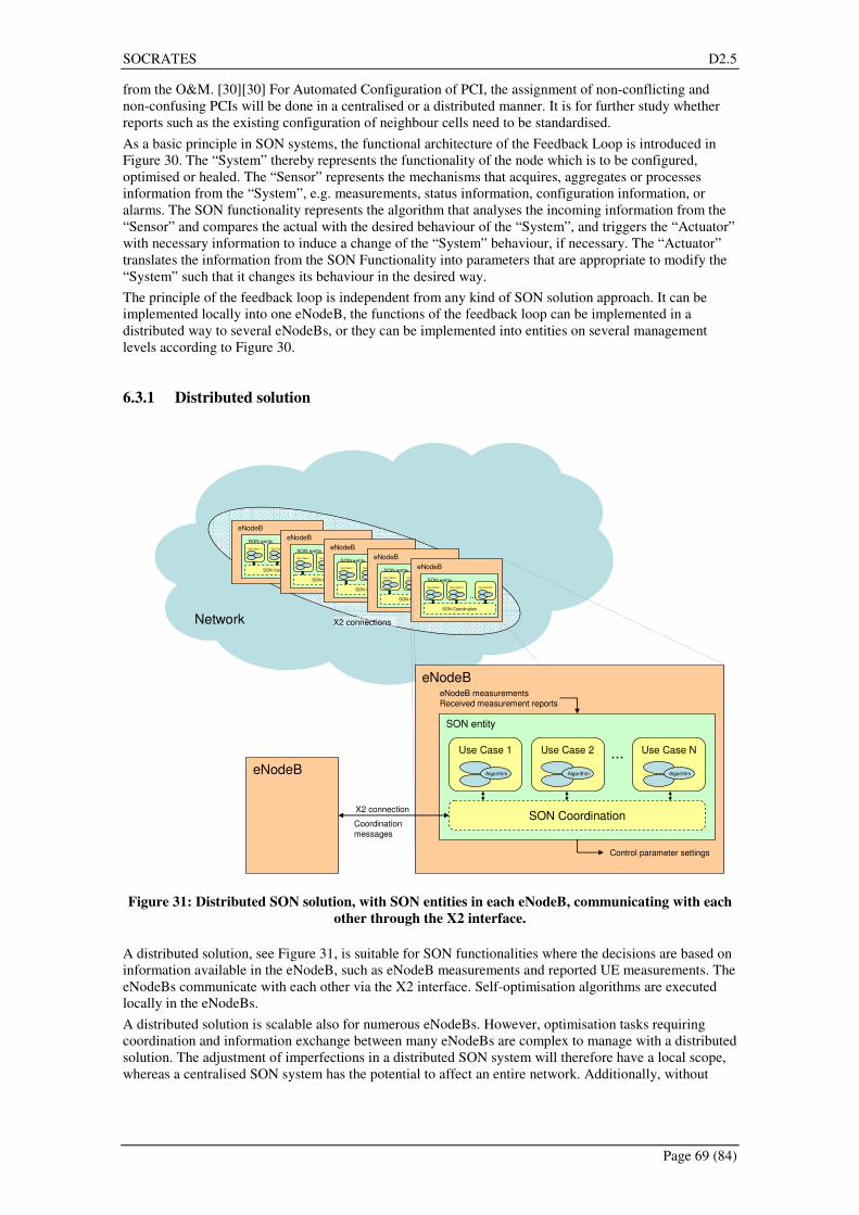
SOCRATES D2.5

(84)

from the O&M. [30][30] For Automated Configuration of PCI, the assignment of non-conflicting and

non-confusing PCIs will be done in a centralised or a distributed manner. It is for further study whether

reports such as the existing configuration of neighbour cells need to be standardised.

As a basic principle in SON systems, the functional architecture of the Feedback Loop is introduced in

Figure 30. The “System” thereby represents the functionality of the node which is to be configured,

optimised or healed. The “Sensor” represents the mechanisms that acquires, aggregates or processes

information from the “System”, e.g. measurements, status information, configuration information, or

alarms. The SON functionality represents the algorithm that analyses the incoming information from the

“Sensor” and compares the actual with the desired behaviour of the “System”, and triggers the “Actuator”

with necessary information to induce a change of the “System” behaviour, if necessary. The “Actuator”

translates the information from the SON Functionality into parameters that are appropriate to modify the

“System” such that it changes its behaviour in the desired way.

The principle of the feedback loop is independent from any kind of SON solution approach. It can be

implemented locally into one eNodeB, the functions of the feedback loop can be implemented in a

distributed way to several eNodeBs, or they can be implemented into entities on several management

levels according to Figure 30.

6.3.1 Distributed solution

eNodeB

SON entity

Use Case 1

Algorith

m

Use Case 2

Algorit h

m

Use Case N

Algorith

m

...

SON Coordination

eNodeB

SON entity

Use Case 1

Algorith

m

Use Case 2

Algori th

m

Use Case N

Algorit h

m

...

SON Coordination

eNodeB

SON entity

Use Case 1

Algorit h

m

Use Case 2

Algori th

m

Use Case N

Algori th

m...

SON Coordination

eNodeB

SON entity

Use Case 1

Algorith

m

Use Case 2

Algorith

m

Use Case N

Algorith

m

...

SON Coordination

eNodeB

SON entity

Use Case 1

Algorit h

m

Use Case 2

Algorith

m

Use Case N

Algori th

m

...

SON Coordination

X2 connectionsNetwork

eNodeB

SON entity

Use Case 1

Algorithm

Use Case 2

Algorithm

Use Case N

Algorithm

...

SON CoordinationX2 connection

eNodeB measurements

Received measurement reports

Control parameter settings

Coordination

messages

eNodeB

Figure 31: Distributed SON solution, with SON entities in each eNodeB, communicating with each

other through the X2 interface.

A distributed solution, see Figure 31, is suitable for SON functionalities where the decisions are based on

information available in the eNodeB, such as eNodeB measurements and reported UE measurements. The

eNodeBs communicate with each other via the X2 interface. Self-optimisation algorithms are executed

locally in the eNodeBs.

A distributed solution is scalable also for numerous eNodeBs. However, optimisation tasks requiring

coordination and information exchange between many eNodeBs are complex to manage with a distributed

solution. The adjustment of imperfections in a distributed SON system will therefore have a local scope,

whereas a centralised SON system has the potential to affect an entire network. Additionally, without

SOCRATES D2.5

(84)

central management it may happen that eNodeBs will continuously exchange conflicting messages and no

proper action will be performed unless a conflict handling is implemented.

A special case of the distributed SON solution is the Localised SON solution, where the optimisation

scope is only one cell or at least one eNodeB. The eNodeB may need some measurements or information

from other eNodeBs, but no information exchange for coordination purpose is necessary. For all use cases

where this local scope applies, the Localised SON solution has the advantage of potential faster update

rate and the possibility of short-term statistics, for example.

6.3.2 Centralised solution

In the Centralised SON solution approach, all optimisation algorithms are executed in a Central Node,

which is most reasonably located close to or within the OAM system. The SON functionality therefore

resides in a small number of locations at a higher management level.

eNodeBeNodeB

eNodeBeNodeB

eNodeB

Central Node

SON entity

Use Case 1

Algorithm

Use Case 2

Algorithm

Use Case N

Algorithm...

SON Coordination

e NodeB measurements



Network

Figure 32: Centralised SON solution, with one SON entity on a central node managing the

interaction between the eNodeBs.

Centralised SON functionality, see Figure 32, could be suitable in cases where there is a need to manage

and survey the interaction between many different cells. This is in principle also possible with a

distributed solution, but in that case there might occur a considerable signalling overhead The self-

organising mechanisms are performed only in the central node, separate eNodeBs do not take any

independent actions apart from the exchange of Key Performance Indicators (KPI), measurements and

signalling messages with the SON entity. The communication with the eNodeB is handled over the OAM

interface.

6.3.3 Hybrid solution

A combination of the distributed and the centralised solution, denoted as Hybrid SON solution, see Figure

33, may be useful when many of the self-organisation tasks (especially those with local scope, i.e., one or

a few cells) can be performed in the eNodeBs themselves, but some tasks (especially complex tasks

where many cells or the whole system are affected) need to be managed from a central node. This

SOCRATES D2.5

(84)

solution can benefit from two parent mechanisms, centralised and distributed solution, but needs a proper

division of the responsibilities between the central and the distributed SON entities.

eNodeB

SON entity

Use Case 1

Algorith

m

Use Case 2

Algorit h

m

Use Case N

Al gorith

m

...

SON Coordination

eNodeB

SON entity

Use Case 1

Algorit h

m

Use Case 2

Algorith

m

Use Case N

Algorith

m

...

SON Coordination

eNodeB

SON entity

Use Case 1

Algorith

m

Use Case 2

Algorith

m

Use Case N

Algorith

m

...

SON Coordination

eNodeB

SON entity

Use Case 1

Algori th

m

Use Case 2

Al gorith

m

Use Case N

Algorith

m

...

SON Coordination

eNodeB

SON entity

Use Case 1

Algorith

m

Use Case 2

Algorit h

m

Use Case N

Algorith

m

...

SON Coordination

X2 connections

NetworkeNodeB

SON entity

Use Case 1

Algorithm

Use Case 2

Algorithm

Use Case N

Algorithm

...

SON Coordination

X2 connection

eNodeB measurements



Coordination

messages

Central Node

SON entity

Use Case 1

Algorithm

Use Case 2

Algorithm

Use Case N

Algorithm...

SON Coordination

e NodeB measurements



Centralized solution

eNodeB

Distributed

solution

Figure 33: Hybrid SON solution, with distributed SON entities in each eNodeB, and a central SON

entity managing the interaction between the eNodeBs.

6.4 Solution selection

As mentioned in the introduction of this chapter, there has been no selection made yet in the SOCRATES

project, which of the presented SON solutions is most in favour for implementation. This has to be

performed in SOCRATES WP3 and WP4 by evaluating each of the SOCRATES use cases and then

extracting a common solution from the individual results. A number of aspects have to be taken into

account when the SON solutions are evaluated from the individual use case view:

• Frequency of input and output to the algorithms

• Number of and location of input sources to the SON functionality

• Interdependencies (measurements, signalling exchange) between nodes related to the SON

functionality

• Number of nodes involved in the SON functionality

• Knowledge of all involved nodes in the network

• Bandwidth requirements on the feedback loop

• Requirements on data storage for long-term analysis

• Probability of unexpected events (for example, the probability for on-off switching of the nodes

is relatively high for home eNodeBs)

• Multivendor aspects

• OPEX/CAPEX effects

• Interaction with other SON algorithms

It is recommended that for each of the use cases worked on within the SOCRATES project, an evaluation

is performed by taking into account the previously described aspects, to derive the architecture solution

which is the most suitable for this use case. By taking the results from all use cases it should then be able

to draw a general SOCRATES recommendation on a SON architecture.

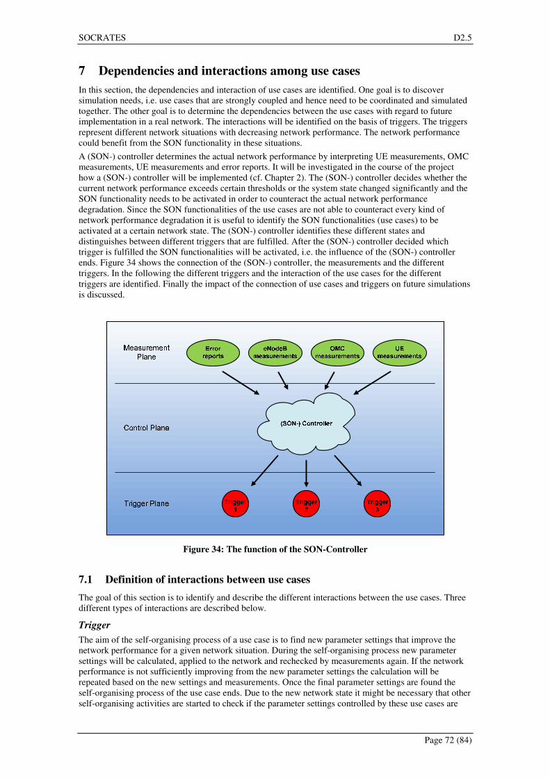
SOCRATES D2.5

(84)

7 Dependencies and interactions among use cases

In this section, the dependencies and interaction of use cases are identified. One goal is to discover

simulation needs, i.e. use cases that are strongly coupled and hence need to be coordinated and simulated

together. The other goal is to determine the dependencies between the use cases with regard to future

implementation in a real network. The interactions will be identified on the basis of triggers. The triggers

represent different network situations with decreasing network performance. The network performance

could benefit from the SON functionality in these situations.

A (SON-) controller determines the actual network performance by interpreting UE measurements, OMC

measurements, UE measurements and error reports. It will be investigated in the course of the project

how a (SON-) controller will be implemented (cf. Chapter 2). The (SON-) controller decides whether the

current network performance exceeds certain thresholds or the system state changed significantly and the

SON functionality needs to be activated in order to counteract the actual network performance

degradation. Since the SON functionalities of the use cases are not able to counteract every kind of

network performance degradation it is useful to identify the SON functionalities (use cases) to be

activated at a certain network state. The (SON-) controller identifies these different states and

distinguishes between different triggers that are fulfilled. After the (SON-) controller decided which

trigger is fulfilled the SON functionalities will be activated, i.e. the influence of the (SON-) controller

ends. Figure 34 shows the connection of the (SON-) controller, the measurements and the different

triggers. In the following the different triggers and the interaction of the use cases for the different

triggers are identified. Finally the impact of the connection of use cases and triggers on future simulations

is discussed.

Figure 34: The function of the SON-Controller

7.1 Definition of interactions between use cases

The goal of this section is to identify and describe the different interactions between the use cases. Three

different types of interactions are described below.

Trigger

The aim of the self-organising process of a use case is to find new parameter settings that improve the

network performance for a given network situation. During the self-organising process new parameter

settings will be calculated, applied to the network and rechecked by measurements again. If the network

performance is not sufficiently improving from the new parameter settings the calculation will be

repeated based on the new settings and measurements. Once the final parameter settings are found the

self-organising process of the use case ends. Due to the new network state it might be necessary that other

self-organising activities are started to check if the parameter settings controlled by these use cases are

SOCRATES D2.5

(84)

still reasonable. Hence these self-organising processes should be started after the first process ends, i.e.

the first process triggers the other processes. Since the first process is already completed at the time the

second process starts it is not necessary to simulate these use cases together. This means that it is not

necessary to simulate use cases together that interact by triggering each other.

Co-operate

If the network performance decreases the SON functionality of the future networks will be activated to

counteract the network degradation. It is most likely that the self-organisation of more than one use case

may help to improve the network performance by changing different parameter settings. If several use

cases are active in parallel and try to compensate the same problem this will be called; the use cases co-

operate on the same problem. To coordinate the different self-organisation activities an intensive

information exchange between the use cases is necessary. The involved use cases will need to be

simulated together in simulations, i.e. use cases that interact by co-operating on the same problem need to

be simulated together.

Co-act

Different self-organising processes that change the same parameter settings may be active in parallel.

These processes can be activated by different triggers. That means the associated use cases do not co-

operate on the same problem, but co-act on the same parameter settings. This interaction might lead to

configuration loops in the self-organising activities where parameter settings are changed repeatedly due

to different triggers. For future simulations and the implementation of the algorithms into the network it is

necessary to simulate these use cases together that co-act on the same parameter settings. This interaction

will not be identified by the dependencies and interaction between use cases. More information about this

interaction can be found in Chapter 3.

7.2 Connection of use cases and triggers

In order to identify the connection among use cases and triggers, a number of network situations that

make self-organising processes beneficial have been identified. In this document these network situations

will be called triggers. They will be derived from measurements which are interpreted by a (SON-)

controller in the LTE networks. The measurements that will be taken into account for each trigger will be

defined at a later time in work package 3 and 4. The follow-up document will be updated according to the

later findings. The following triggers have been identified:

• Low/High number of blocked calls

• Low/High number of dropped calls

• Low/High/Imbalanced quality of service

• Low/High/Imbalanced traffic load

• Low/High Cell capacity

• New site

• Coverage hole

• Cell outage

Figure 35: Legend

SOCRATES D2.5

(84)

Figure 35 explains different symbols that will be used in the following figures. The symbols show the

interaction of use cases and triggers. The co-operation of use cases that is defined in section 5.1 is

visualised by light blue bubbles and the arrow between two use cases indicates that the first use case

triggers the second. That means that the self-organising process of the first use case has to be completed

before the next process is started. The algorithms that will be developed in some use cases will have to be

integrated in the (SON-) controller since they check the network continuously to detect coverage holes or

cells in outage which are triggers for SON processes. These use cases are marked by a red border. It will

have to be decided at a later time how this integration will look like.

Trigger: Blocked Calls

If the number of blocked calls in a cell area is low it might make sense to trigger the use case ‘Reduction

of energy consumption’ to check if it is possible to turn off certain network elements (Figure 36, Element

1). The fact that the number of blocked calls is low will not be the only indication for this use case to

switch off equipment but is a necessary condition. It will be decided later in the development of the

algorithms for this use case how the different indicators will be taken into account. There might be the

restriction that network elements may only be switched off during night time, for example.

low

high

Figure 36: Blocked Calls

A high number of blocked calls activate the use case ‘Reduction of energy consumption’ as well (Figure

36, Element 2). This time it has to be checked if any equipment is turned off before the compensation

starts, because this might lead to an increased number of blocked calls. If no network element is switched

off the use case ‘Self-optimisation of home eNodeB’ is triggered (Figure 36, Element 3). This is because

it was stated that no changes should be done to the network because of problems that occur due to the

presence of home eNodeBs. If many home eNodeBs need to be coordinated with the cell, the amount of

signalling traffic increases, e.g. due to an increased number of handovers between the network and the

home eNodeBs. This could lead to blocked calls in the cell because resources like the RACH could be

busy handling the handovers if the handover thresholds of the home eNodeBs are not set reasonably. The

‘Self-optimisation of home eNodeB’ triggers the blue bubble if the problem is not solved (Figure 36,

Element 4).

The use cases ‘Admission control’, ‘Load balancing’, ‘Handover optimisation’ and ‘RACH optimisation’

co-operate on the problem of a high number of blocked calls. As stated before intensive information

exchange between these use cases will be necessary to coordinate the self-organisation functionality. The

‘Self-optimisation of physical channels’ is triggered if the problem could be solved by the co-operating

use cases because the changes to the network might be essential and the network performance could

benefit from new parameter settings of the physical channels (Figure 36, Element 5). If the problem is not

SOCRATES D2.5

(84)

solved and occurs more often it will most likely be necessary to add new hardware. In this case the use

case ‘Intelligently selecting site location’ will be triggered to propose a site location for the new

equipment (Figure 36, Element 6).

Trigger: Dropped Calls

If the number of dropped calls in a cell area is low it might make sense to trigger the use case ‘Reduction

of energy consumption’ to check if it is possible to turn off certain network elements (Figure 37, Element

1). The fact that the number of dropped calls is low will not be the only indication for this use case to




A high number of dropped calls activate the use case ‘Reduction of energy consumption’ as well (Figure

37, Element 2). This time it has to be checked if any equipment is turned off before the compensation

starts because this might lead to an increased number of drooped calls. If no network elements are

switched off the use case ‘Self-optimisation of home eNodeB’ is triggered (Figure 37, Element 3). This is

because it was stated that no changes should be done to the network because of problems that occur due

to the presence of home eNodeBs. If home eNodeBs are present in a cell area it might happen that calls

are dropped because the handovers to or from the home eNodeBs fail. Incorrect entries in the neighbour

lists could be a reason for that. Another reason for dropped calls could be the interference of home

eNodeBs that leads to dropped calls in the surrounding cell.

The use case ‘Coverage hole detection’ is triggered by the ‘Reduction of energy consumption’ as well

(Figure 37, Element 4). It is obvious that a call is dropped if an UE leaves the cell area and enters an

uncovered area. Hence it should be checked first if a coverage hole causes the dropped calls. If a coverage

hole is found the use case ‘Coverage hole compensation’ is triggered (Figure 37, Element 5). The blue

bubble is only triggered if the dropped calls where not caused by the presence of home eNodeBs and no

coverage holes were found or the coverage holes were compensated (Figure 37, Element 6).

The use cases ‘Congestion Control’, ‘Admission control’, ‘Interference Coordination’, ‘Load balancing’

and ‘Handover optimisation’ co-operate on the problem of a high number of dropped calls. As stated

before intensive information exchange between these use cases will be necessary to coordinate the self-

organisation functionality. The ‘Self-optimisation of physical channels’ (Figure 37, Element 7) and the

‘RACH optimisation’ (Figure 37, Element 8) are triggered if the problem could be solved by the co-

operating use cases. The changes to the network might be essential and the network performance could

benefit from new settings of the physical channels and RACH parameters. If the problem was not solved

and occurs more often it will most likely be necessary to add new hardware. In this case the use case

‘Intelligently selecting site location’ will be triggered to propose a site location for the new equipment

(Figure 37, Element 9).

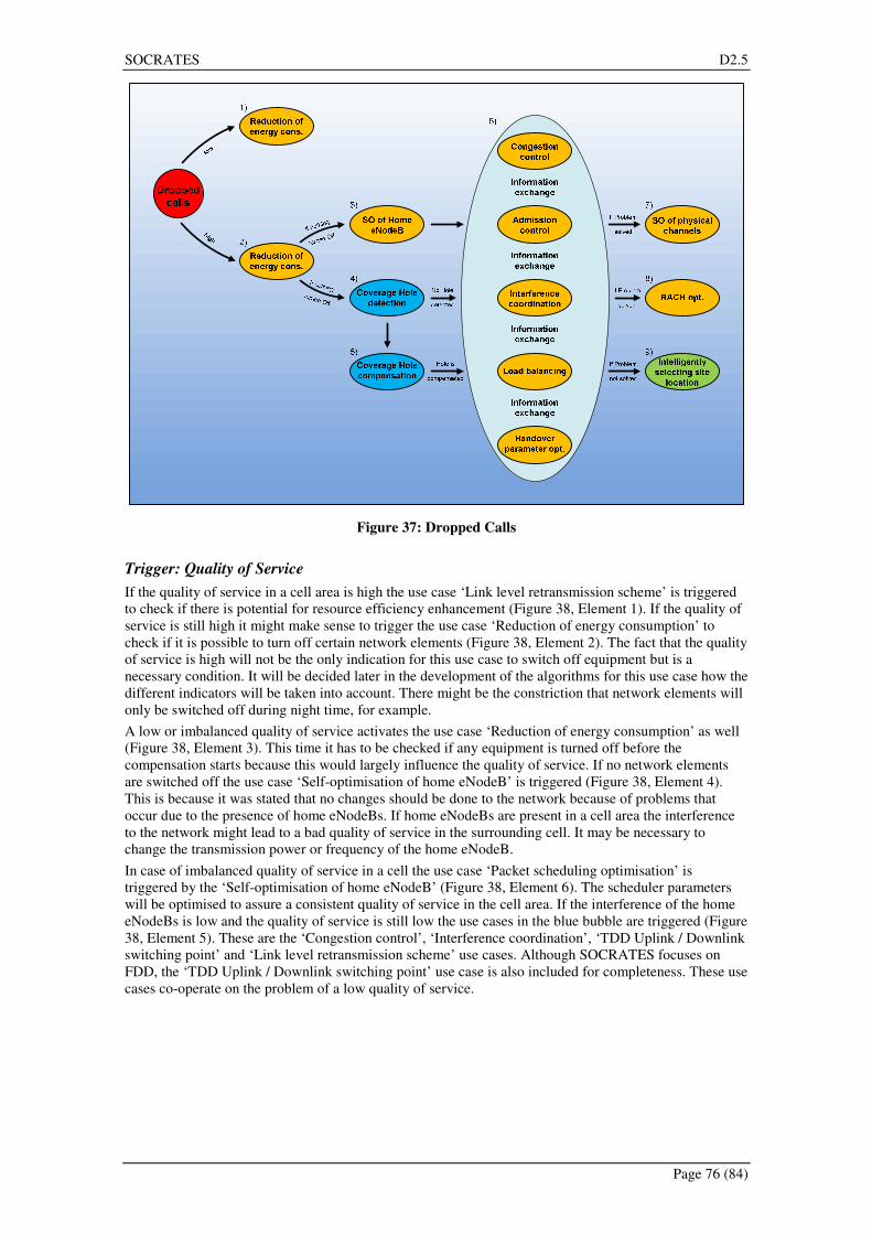
SOCRATES D2.5

(84)

Figure 37: Dropped Calls

Trigger: Quality of Service

If the quality of service in a cell area is high the use case ‘Link level retransmission scheme’ is triggered

to check if there is potential for resource efficiency enhancement (Figure 38, Element 1). If the quality of

service is still high it might make sense to trigger the use case ‘Reduction of energy consumption’ to

check if it is possible to turn off certain network elements (Figure 38, Element 2). The fact that the quality

of service is high will not be the only indication for this use case to switch off equipment but is a

necessary condition. It will be decided later in the development of the algorithms for this use case how the

different indicators will be taken into account. There might be the constriction that network elements will

only be switched off during night time, for example.

A low or imbalanced quality of service activates the use case ‘Reduction of energy consumption’ as well

(Figure 38, Element 3). This time it has to be checked if any equipment is turned off before the

compensation starts because this would largely influence the quality of service. If no network elements

are switched off the use case ‘Self-optimisation of home eNodeB’ is triggered (Figure 38, Element 4).

This is because it was stated that no changes should be done to the network because of problems that

occur due to the presence of home eNodeBs. If home eNodeBs are present in a cell area the interference

to the network might lead to a bad quality of service in the surrounding cell. It may be necessary to

change the transmission power or frequency of the home eNodeB.

In case of imbalanced quality of service in a cell the use case ‘Packet scheduling optimisation’ is

triggered by the ‘Self-optimisation of home eNodeB’ (Figure 38, Element 6). The scheduler parameters

will be optimised to assure a consistent quality of service in the cell area. If the interference of the home

eNodeBs is low and the quality of service is still low the use cases in the blue bubble are triggered (Figure

38, Element 5). These are the ‘Congestion control’, ‘Interference coordination’, ‘TDD Uplink / Downlink

switching point’ and ‘Link level retransmission scheme’ use cases. Although SOCRATES focuses on

FDD, the ‘TDD Uplink / Downlink switching point’ use case is also included for completeness. These use

cases co-operate on the problem of a low quality of service.

SOCRATES D2.5

(84)

lowimbalance

high

Figure 38: Quality of Service

As stated before intensive information exchange between these use cases will be necessary to coordinate

the self-organisation functionality. The ‘Self-optimisation of physical channels’ (Figure 38, Element 7)

and the ‘Handover optimisation’ (Figure 38, Element 8) are triggered if the problem could be solved by

the co-operating use cases. The changes to the network might be essential and the network performance

could benefit from new settings of the physical channels and Handover parameters.

If the quality of service is low more often in the same cell area the use case ‘Tracking areas’ is activated

(Figure 38, Element 9). Due to the fact that tracking area updates require network capacity it might make

sense to change the tracking areas. The ‘RACH optimisation’ use case is triggered if the tracking areas

are changed because the tracking area updates need the RACH and hence the network performance could

benefit from a RACH parameter update (Figure 38, Element 11). If the problem was not solved and

occurs more often it will most likely be necessary to add new hardware. In this case the use case



Trigger: Traffic Load

If the traffic load in a cell area is low it might make sense to trigger the use case ‘Reduction of energy

consumption’ to check if it is possible to turn off certain network elements (Figure 39, Element 1). The

fact that the traffic load is low will not be the only indication for this use case to switch off equipment but

is a necessary condition. It will be decided later in the development of the algorithms for this use case

how the different indicators will be taken into account. There might be the constriction that network

elements will only be switched off during night time, for example.

A high or imbalanced traffic load activates the use case ‘Reduction of energy consumption’ as well

(Figure 39, Element 2). This time it has to be checked if any equipment is turned off before the

compensation starts. The capacity of the cell might be small because some equipment was turned off. If

no network elements are switched off the use cases ‘Congestion Control’ and ‘TDD Uplink / Downlink

switching point’ are triggered in the case of high traffic load (Figure 39, Element 3) to handle the load.

Although SOCRATES focuses on FDD, the ‘TDD Uplink / Downlink switching point’ use case is also

included for completeness. If the traffic load is imbalanced the use cases ‘TDD Uplink / Downlink

switching point’ and ‘Load balancing’ are triggered (Figure 39, Element 4). The aim of these use cases is

to balance the load and change the bandwidth of the uplink or downlink to avoid bad quality of service,

blocked and dropped calls.

The handover parameters need to be checked whenever the network is changed essentially (Figure 39,

Element 6). If the traffic load is high more often in the same cell area the use case ‘Tracking areas’ is

activated (Figure 39, Element 5). Due to the fact that tracking area updates require network capacity it

might make sense to change the tracking areas. The ‘RACH optimisation’ use case is triggered if the

SOCRATES D2.5

(84)

tracking areas are changed because the tracking area updates need the RACH and hence the network

performance could benefit from a RACH parameter update (Figure 39, Element 7). If the problem was

not solved and occurs more often it will most likely be necessary to add new hardware. In this case the

use case ‘Intelligently selecting site location’ will be triggered to propose a site location for the new

equipment (Figure 39, Element 8).

Figure 39: Traffic Load

Trigger: Cell Capacity

If the amount of unused cell capacity of a certain cell is high it might make sense to trigger the use case

‘Reduction of energy consumption’ to check if it is possible to turn off certain network elements (Figure

40, Element 1). The fact that the cell capacity is high will not be the only indication for this use case to




A low cell capacity activates the use case ‘Reduction of energy consumption’ as well (Figure 40, Element

2). This time it has to be checked whether any equipment is turned off before compensation actions start,

because the observed low cell capacity may simply be due to switched off eNodeBs. If no network

elements are switched off the use case ‘Self-optimisation of home eNodeB’ is triggered (Figure 40,

Element 3). This is because it was stated that no changes should be done to the network because of

problems that occur due to the presence of home eNodeBs. If home eNodeBs are present in a cell area it

might happen that the cell capacity decreases due to interference from the home eNodeBs. If this is the

case the home eNodeBs should reconfigures to solve the problem before the network parameters are

changed.

The use case ‘Interference coordination’ is triggered if the home eNodeBs didn’t cause the problem of a

low cell capacity (Figure 40, Element 4). The self-organisation functionality of this use case will decrease

the interference between neighbouring cells to increase the cell capacity. If the problem was not solved

and occurs more often it will most likely be necessary to add new hardware. In this case the use case


(Figure 40, Element 5). The ‘Handover parameter optimisation’ (Figure 40, Element 6) and the ‘RACH

optimisation’ (Figure 40, Element 7) are triggered if the problem could be solved by the ‘Interference

coordination’ use case. The changes to the network might be essential and the network performance could

benefit from new settings of the handover and RACH parameters.

SOCRATES D2.5

(84)

low

high

Figure 40: Cell Capacity

Trigger: New Site

The use cases ‘Interference coordination’, ‘Load balancing’, ‘Handover parameter optimisation’ and

‘Coverage hole detection’ are the main contributors to the decision that a new site is needed (Figure 41,

Element 1). If the interference in a cell area is high, the traffic load can not be handled or balanced,

changed handover parameters can not solve the problem or coverage holes are detected and these effects

are observed over a significant time period it will be necessary to add new hardware. The trigger new site

will be fulfilled in this case. The use case ‘Intelligently selecting site location’ will be activated to

propose a new site location (Figure 41, Element 2).

If the problem is limited to a small area or might only be an indoor problem the insertion home eNodeB

could solve the problem (Figure 41, Element 3). In this case the ‘Intelligently selecting site location’ use

case would propose to add a home eNodeB and the use case ‘Self-optimisation of home eNodeB’ would

be triggered at the start-up of the new home eNodeB. If the problem cannot be solved by a home eNodeB

a new site has to be deployed. The time between the proposal of a new site location and the new site

being deployed will most likely be month or years depending on the urgency of the problem.

If it is proposed to solve the problem by a relay or repeater the use case ‘Management of Relays and

Repeaters’ will be triggered during the start-up of the hardware (Figure 41, Element 5). The ‘Automatic

generation of default parameters’ use case is activated if a new eNodeB is deployed (Figure 41, Element

4). The ‘Self-optimisation of physical channels’ (Figure 41, Element 6) and ‘Tracking areas’ (Figure 41,

Element 7) use cases are triggered because essential changes to the network have a great impact on the

physical channels and tracking area parameters. The ‘RACH optimisation’ use case is triggered if the

tracking areas are changed because the tracking area updates need the RACH and hence the network

performance could benefit from a RACH parameter update (Figure 41, Element 8).

SOCRATES D2.5

(84)

Figure 41: New Site

Trigger: Coverage Hole

In future LTE networks the coverage holes will be detected automatically by the algorithms developed for

the ‘Coverage hole detection’ use case (Figure 42, Element 1). As mentioned before these algorithms will

most likely be integrated into the control layer (Figure 34) as their findings lead to triggers that start SON

processes. The ‘Coverage hole compensation’ use case is triggered if a coverage hole was detected

(Figure 42, Element 2). The coverage hole compensation aims at compensating the coverage holes in the

long run without adding new hardware. If the coverage hole can not be compensated and no equipment is

in outage it will be necessary to add new hardware. In this case the use case ‘Intelligently selecting site

location’ will be triggered to propose a site location for the new equipment (Figure 42, Element 3). The

‘Tracking areas’ (Figure 42, Element 4) and ‘Handover parameter optimisation’ (Figure 42, Element 5)

use cases are triggered if the coverage hole was compensated successfully because essential changes to

the network have a great impact on the tracking area and handover parameter settings. The ‘RACH

optimisation’ use case is triggered if the tracking areas are changed because the tracking area updates

need the RACH and hence the network performance could benefit from a RACH parameter update


Figure 42: Coverage Hole

SOCRATES D2.5

(84)

Trigger: Cell Outage

The use case ‘Cell outage prediction’ tries to predict cell outages by long-term observations of the

hardware and software error reports, the temperature of the hardware, or the traffic load etc. (Figure 43,

Element 1). The aim is to provide the ‘Cell outage detection’ use case with information about a potential

cell outage, which makes it easier to detect a cell outage. The ‘Cell outage detection’ is triggered if a cell

outage is most likely to occur soon (Figure 43, Element 2). The ‘Cell outage detection’ exchanges

information with the ‘Cell outage prediction’ if a cell outage was detected to improve the cell outage

prediction (Figure 43, Element 3).

Figure 43: Cell Outage

As mentioned before the algorithms of the ‘Cell outage prediction’ and ‘Cell outage detection’ use case

will most likely be integrated into the control layer (Figure 34) as their findings lead to triggers that start

SON processes. If a cell outage was detected the ‘Cell outage compensation’ use case is triggered (Figure

43, Element 4). The SON functionality of this use case tries to compensate the cell outage for short-term

until the necessary repairs are done. The compensation activities may include network performance

degradations in surrounding cells. The ‘Self-optimisation of physical channels’ (Figure 43, Element 5),

‘Tracking areas’ (Figure 43, Element 6) and ‘Handover parameter optimisation’ (Figure 43, Element 7)

use cases are triggered because essential changes to the network have a great impact on the physical

channels, tracking area and handover parameter settings. The ‘RACH optimisation’ use case is triggered

if the tracking areas are changed because the tracking area updates need the RACH and hence the network

performance could benefit from a RACH parameter update (Figure 43, Element 8).

SOCRATES D2.5

(84)

QoSTraffic

LoadBlocked

Calls

Measurement

Plane

Control Plane

Trigger Plane Dropped

Calls

Self-

Organisation

Plane

Funct.

2

Funct.

3

Funct.

4

Funct.

5

Coordination

Plane

Parameter Plane

Funct.

6

Funct.

1

Funct.

7

Funct.

5

Funct.

1

New

Site

Cov.

Hole

Cell

outageCapacity

Funct.

x. . .

Funct.

x2. . .

Funct.

6

Funct.

8

UE

measurements

OMC

measurements

Error

reports

(SON-) Controller

eNodeB

measurements

Operator

policy

(SON-) Coordinator

Parameter 2Parameter 1 Parameter x…

Operator

policy

Figure 44: The overall system

Figure 44 shows the overall system including the SON functionality. The (SON-) controller can be

influenced by the operator through operator policies. All triggers that were identified are added to the

trigger plane. The self-organisation plane includes all SON functions initiated by the triggers. Figure 44

only gives a schematic overview of the possible interactions of the SON functions in this plane. A more

detailed description of the interactions based on the triggers can be found in Figure 36 - Figure 43.

Operator policies are taken into account in the coordination plane. This plane includes the conflict

handling described in section 4.3 of deliverable D2.4 and will avoid self-organisation loops. The (SON-)

coordinator will also be able to monitor the success of the SON functionalities and give feedback to the

SON functions. The new parameter settings found by the SON functions will only be applied to the

network if no conflicts are detected.

SOCRATES D2.5

(84)

8 References

[1] “Use Cases for Self-Organising Networks”, SOCRATES deliverable D2.1, March 2008.

[2] “Requirements for Self-Organising Networks”, SOCRATES deliverable D2.2, June 2008.

[3] “Assessment criteria for self-organising networks”, SOCRATES deliverable D2.3, June 2008.

[4] “Framework for the development of self-organisaiton methods”, SOCRATES deliverable D2.4,

September 2008.

[5] 3GPP TS 36.214, Evolved Universal Terrestrial Radio Access (E-UTRA); Physical Layer

Measurements (Release 8); Sept. 2008.

[6] I. Viering, M. Döttling and A. Lobinger, "A mathematical perspective of self-optimizing

wireless networks", submitted to the IEEE International Conference on Communications 2009,

Dresden, Germany, June 2009, accepted.

[7] “Next Generation Mobile Networks Radio Access Performance Evaluation Methodology”,

NGMN white paper, June 2007.

[8] 3GPP TR 25.892, Feasibility Study for Orthogonal Frequency Division Multiplexing (OFDM)

for UTRAN enhancement.

[9] “The E-model, a Computational Model for use in Transmission Planning”, ITU-T Rec. G.107,

March 2005.

[10] R. Jain, D. Chiu and W. Hawe, “A Quantitative Measure of Fairness and Discrimination for

Resource Allocation in Shared Computer Systems”, Technical Report DEC-TR-301, DEC,

Sept. 1984.

[11] “Evaluation Methodology Document (EMD)”, IEEE 802.16m-08/004r1, March 2008.

[12] “Multi-hop Relay System Evaluation Methodology (Channel Model and Performance

Metric)”, IEEE 802.16j-06/013r3, February 2007.

[13] T. Chen, M. Kuusela and E. Malkamaki, “Uplink Capacity of VoIP on HSUPA”, Proceedings

of VTC ’06 (Spring), Melbourne, Australia, 2006.

[14] H. Holma and A. Toskala (eds.), “HSDPA/HSUPA for UMTS”, John Wiley & Sons,

Chichester, United Kingdom, 2006.

[15] R. Litjens, “A Flow Level Capacity Comparison of UMTS and HSDPA”, Proceedings of

MSWiM ’05, Montreal, Canada, 2005.

[16] R. Litjens, “The Impact of Mobility on UMTS Network Planning'', Computer networks, Vol.

38, No. 4, 2002.

[17] L. Ferreira (ed.), L.M. Correia, A. Serrador, G. Carvalho, E. Fledderus and R. Perera, “UMTS

Deployment and Mobility Scenarios”, IST MOMENTUM Project, Deliverable D1.3, IST-

TUL, Lisbon, Portugal, October 2002.

[18] L. Ahlin, J. Zander and B. Slimane. “Principles of Wireless Communications”,

Studentlitteratur, ISBN 91-44-03080-0, 2006.

[19] “Digital Mobile Radio towards Future Generation Systems”, COST 231 Final Report.

[20] F. Belloni, “Fading Models, S73.333, Physical Layer Methods in Wireless Communications

Systems”, Helsinki Institute of Technology, November 2004

[21] S.R. Saunders, “Antennas and Propagation for Wireless Communication Systems”, 2nd

edition,

Wiley 2007.

[22] M. Gudmundson, “Correlation Model for Shadow Fading in Mobile Radio Systems”,

Electronic Letters, 27, 2145-2146, 1991.

[23] “3rd

Generation Partnership Project; Technical Specification Group Radio Access Network;

Spatial Channel Model for MIMO Simulations (Release 7)”, V7.0.0., 3GPP TR 25.996.

[24] WINNER, Wireless World Initiative New Radio, www.ist-winner.org.

[25] P. Kyosti, “Matlab SW Documentation of WIM2 Model”.

[26] “3rd

Generation Partnership Project; Technical Specification Group Radio Access Network;

Physical Layer Aspects for Evolved Universal Terrestrial Radio Access (UTRA) (Release 7)”,

V7.1.0, 3GPP TR 25.814.

[27] 3GPP TS 32.101: Telecommunication Management; Principles and High-level Requirements

(Release 8); Version 8.2.0, June 2008

SOCRATES D2.5

(84)

[28] 3GPP TS 36.420: Evolved Universal Terrestrial Radio Access Network (E-UTRAN); X2

general aspects and principles; Version 8.0.0, December 2007

[29] 3GPP TR 23.882: 3GPP System Architecture Evolution (SAE): Report on Technical Options

and Conclusions (Release 7); Version 1.5.0, November 2006

[30] 3GPP TS 36.300: Evolved Universal Terrestrial Radio Access (E-UTRA) and Evolved

Universal Terrestrial Radio Access Network (E-UTRAN); Overall description; Stage 2

(Release 8); Version 8.7.0 December 2008

[31] Eisenblätter, A., Geerdes, H.-F., Koch, T. (ed.), Türke, U. XML Data Specification and

Documentation, Appendix to Momentum Deliverable 5.2, September 2003.

[32] Eisenblätter, A., Geerdes, H.-F., Türke, U., Koch, T. Momentum Data Scenarios for Radio

Network Planning and Simulation. Proc. WiOpt'04, Cambridge, UK, 2004

[33] Eisenblätter, A., Geerdes, H.-F., Türke, U. Public UMTS radio network evaluation and

planning scenarios. Internat. J. on Mobile Network Design and Innovation, 1(1):40–53, 2005.

[34] Lourenço, P. (ed.), Fledderus, E.R., Geerdes, H.-F., Heideck, B., Kürner, T., Rakoczi, B.,

Reference Scenarios, Momentum Deliverable 5.2, June 2003.

[35] Momentum Project IST-2000-28088: Public UMTS Planning Scenarios.

http://momentum.zib.de (2005)

[36] MORANS activity, Working Group 3 "Radio Networks Aspects" (WG3), COST273 Action,

http://www.buehler.at/morans/ (requires registration)

[37] http://www.openstreetmap.org

[38] NGMN Project 12, Informative List of SON Use Cases, v 1.53 (included in 3GPP S5-071944)

[39] Monotas, http://www.macltd.com/monotas/

[40] 3GPP R4-071231: Open and closed access for Home Node Bs

d2.5 review of use cases and framework public version review of us… · review of use cases and...

Documents