damage assessment for buried pipes affected by …
TRANSCRIPT
DAMAGE ASSESSMENT FOR BURIED PIPES AFFECTED BY GROUND MOTIONS AND LIQUEFACTION IN THE 2011 OFF THE
PACIFIC COAST OF TOHOKU EARTHQUAKE
Gaku SHOJI1, Reina KOBAYASHI 2, Masahiro HARA3
ABSTRACT This study examined the dependence of damage of buried pipes used for water supply systems and sewer systems in the 2011 off the Pacific coast of Tohoku earthquake on the strong motion intensities obtained for liquefied and non-liquefied grounds at Kamisu City in Ibaraki Prefecture, Japan. The relations between the damage ratio and the ground motion intensities were reasonably explained by classifying the targeted sites by the soil properties. The modeling of associated fragility curves were also attempted with respect to the peak ground velocity by classifying the value of potential liquefaction for the targeted sites Keywords: Buried pipe; Seismic damage; the 2011 off the Pacific coast of Tohoku earthquake; Liquefaction; Effective stress analysis 1. INTRODUCTION The earthquake off the Pacific coast of Tohoku on March 11th, 2011 (hereinafter referred to as “the Tohoku earthquake”) caused major damage to water supply systems and sewerage systems. According to the Ministry of Health, Labor and Welfare (2013), water outages occurred at a maximum of 2,567,210 houses in 21 prefectures and Tokyo Metropolitan. Additionally, the Ibaraki Prefecture included the maximum number of water outage houses (801,018 houses). Sewerage disruption outages also occurred in 10 prefectures and Tokyo. The Sewerage Technological Examination Committee for Earthquake and Tsunami (2016) indicated that the damaged length of sewer pipes corresponded to 642 km for the total length of the buried sewer pipes (65,001km). Prior to the Tohoku earthquake, several researchers discussed seismic reliability of water supply systems and sewerage systems (for example, Hwang et al. (1998), Liu & Hung (2009), Javanbarg & Takada (2009), Shoji et al. (2011)). Following the Tohoku earthquake, researchers evaluated damages on water supply and sewage systems by various indices of ground motion intensity (for example, Naba et al. (2012), Toprak et al. (2017)). Tsukiji and Shoji (2013) analyzed the dependence of damage ratio of buried distribution pipes on the spatial distribution of peak ground velocity (PGV) at Itako City and Kamisu City in the Ibaraki Prefecture, Japan and derived the associated fragility curves. However, these studies did not focus on site-specific ground motions and liquefaction at the target sites. Detailed analyses under the ground are required to clarify the dependence of pipe damage on ground motion intensity. Unjoh et al. (2013) investigated the effect of seismic ground motions on soil liquefaction by performing a one-dimensional soil response analysis. We follow the same and provide more detailed considerations for the dependence of the pipe damage on the ground motion. The purpose of this study involves analyzing the damage to buried pipes by considering the mechanical properties of the ground. First, we model the soil layers at 39 target sites based on the data from boring
1Associate Prof., Dr.Eng., University of Tsukuba, Tsukuba, Japan, [email protected] 2Graduate Student, Graduate School of Systems and Information Eng., University of Tsukuba, Tsukuba, Japan, [email protected] 3Ditto, [email protected]
2
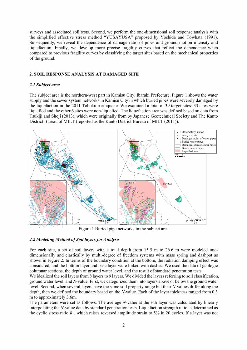
surveys and associated soil tests. Second, we perform the one-dimensional soil response analysis with the simplified effective stress method “YUSAYUSA” proposed by Yoshida and Towhata (1991). Subsequently, we reveal the dependence of damage ratio of pipes and ground motion intensity and liquefaction. Finally, we develop more precise fragility curves that reflect the dependence when compared to previous fragility curves by classifying the target sites based on the mechanical properties of the ground. 2. SOIL RESPONSE ANALYSIS AT DAMAGED SITE 2.1 Subject area The subject area is the northern-west part in Kamisu City, Ibaraki Prefecture. Figure 1 shows the water supply and the sewer system networks in Kamisu City in which buried pipes were severely damaged by the liquefaction in the 2011 Tohoku earthquake. We examined a total of 39 target sites: 33 sites were liquefied and the other 6 sites were non-liquefied. The liquefaction area was defined based on data from Tsukiji and Shoji (2013), which were originally from by Japanese Geotechnical Society and The Kanto District Bureau of MILT (reported as the Kanto District Bureau of MILT (2011)).
Figure 1 Buried pipe networks in the subject area
2.2 Modeling Method of Soil layers for Analysis For each site, a set of soil layers with a total depth from 15.5 m to 26.6 m were modeled one-dimensionally and elastically by multi-degree of freedom systems with mass spring and dashpot as shown in Figure 2. In terms of the boundary condition at the bottom, the radiation damping effect was considered, and the bottom layer and base layer were linked with dashes. We used the data of geologic columnar sections, the depth of ground water level, and the result of standard penetration tests. We idealized the soil layers from 8 layers to 9 layers. We divided the layers referring to soil classification, ground water level, and N-value. First, we categorized them into layers above or below the ground water level. Second, when several layers have the same soil property range but their N-values differ along the depth, then we defined the boundary based on the N-value. Each of the layer thickness ranged from 0.3 m to approximately 3.6m. The parameters were set as follows. The average N-value at the i-th layer was calculated by linearly interpolating the N-value data by standard penetration tests. Liquefaction strength ratio is determined as the cyclic stress ratio RL, which raises reversed amplitude strain to 5% in 20 cycles. If a layer was not
#
##
5-44-8
4-7
4-6 4-5
4-3
4-2
4-1
3-3
3-2
2-6
2-5
2-4
2-3
2-2
2-1
1-8
1-71-4
1-3
1-2
1-1
No.2
No.1
5-14
5-13
5-11
5-10
3-233-22
3-213-20
3-19
3-18
3-17
3-16
3-14
3-12
3-10
0 0.50.25km
#
##
0 1 20.5km
5-44-8
4-7
4-6 4-5
4-3
4-2
4-1
3-3
3-2
2-6
2-5
2-4
2-3
2-2
2-1
1-8
1-71-4
1-3
1-2
1-1
No.2
No.1
5-14
5-13
5-11
5-10
3-233-22
3-213-20
3-19
3-18
3-17
3-16
3-14
3-12
3-10
0 0.50.25km
: Observatory station: Analyzed site: Damaged point of water pipes: Buried water pipes: Damaged span of sewer pipes: Buried sewer pipes: Liquefied area
Site 1-1

3
tested for liquefaction strength, RL was spatially interpolated by the Bridge Design Specifications (2012).
Figure 2 Soil layers model for site 1-1
Initial modulus of rigidity G0 was calculated by Equation (1) as follows:
(1)
where γt denotes unit weight of soil, and g denotes gravity acceleration. If shear modulus wave velocity Vs was unknown, it was estimated by applying the equations based on Bridge Design Specifications (2012) with use of Ni denoting the average of N-value at the i-th layer. Internal frictional angle φ for i-th layer was set by the equations by Hatanaka and Uchida (1996). Coefficient of permeability k was set by Darcy’s rule. It was estimated from the table given by Creager et al. (1945). In the analysis, we used Equation (2) based on the table as follows:
0.0034 . 0.005 2 (2)
If there was no value of D20 since the value was excessively low for measurement, we assumed that D20 corresponds to 0.02. With respect to the site that did not possess sufficient data for the standard penetration test and soil test, we used the data of nearby sites in which soil classification is similar. 2.3 Method and Condition of Analysis We performed a one-dimensional effective stress analysis by using the computer program YUSAYUSA-2 developed by Yoshida and Towhata (1991). With respect to the shear stress τ-strain γ model, we used Hardin-Drnevich model. The hysteresis curve obeys Masing rule. The increase in pore water pressure was calculated by the effective stress path proposed by Ishihara and Towhata (1980). The equation of motion was solved by Newmark’s β scheme with β = 0.25. Permeability was calculated by the following equations that depict the vertical movement of soil particle and water following Biot’s method as follows:
(3a)
0 (3b)
Dep
th[m
]
0
5
10
15
20
25
0 10 20 30 40 50N value
Dr
Dr
Dr
Asc
Asc
Ds
Ds
Ds
Ds
Dr
Asc
Ds
Ground water level
Depth of samples
m1
m2
mi
mi+1
mn+1
mn
k1,C1
ki,Ci
kn,Cn
Dr : Dredged soil (Sandy)Asc : Alluvial sandy clayDs : Diluvial sand
1
2
3
4
5
6
7
8
9
ModelOriginal data
4
0 (3c)
(3d)
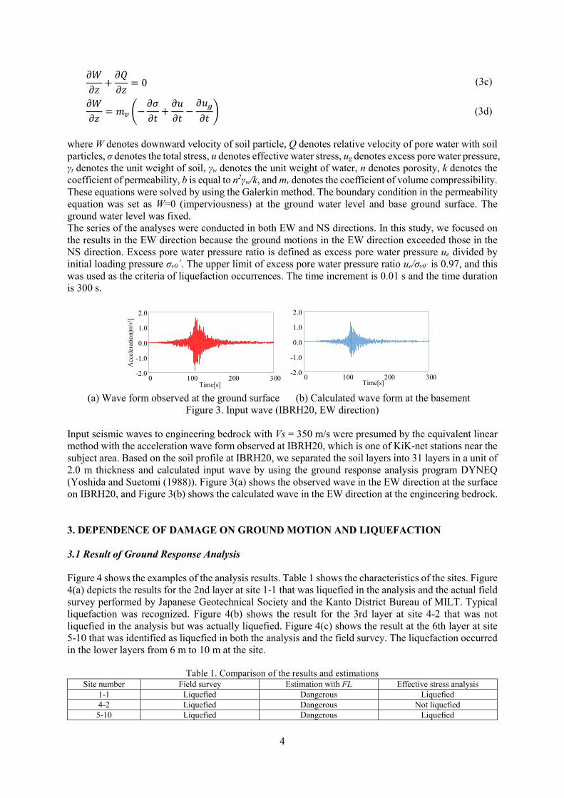
where W denotes downward velocity of soil particle, Q denotes relative velocity of pore water with soil particles, σ denotes the total stress, u denotes effective water stress, ug denotes excess pore water pressure, γt denotes the unit weight of soil, γw denotes the unit weight of water, n denotes porosity, k denotes the coefficient of permeability, b is equal to n2γw/k, and mv denotes the coefficient of volume compressibility. These equations were solved by using the Galerkin method. The boundary condition in the permeability equation was set as W=0 (imperviousness) at the ground water level and base ground surface. The ground water level was fixed. The series of the analyses were conducted in both EW and NS directions. In this study, we focused on the results in the EW direction because the ground motions in the EW direction exceeded those in the NS direction. Excess pore water pressure ratio is defined as excess pore water pressure ue divided by initial loading pressure σv0´. The upper limit of excess pore water pressure ratio ue/σv0´ is 0.97, and this was used as the criteria of liquefaction occurrences. The time increment is 0.01 s and the time duration is 300 s.
(a) Wave form observed at the ground surface (b) Calculated wave form at the basement
Figure 3. Input wave (IBRH20, EW direction) Input seismic waves to engineering bedrock with Vs = 350 m/s were presumed by the equivalent linear method with the acceleration wave form observed at IBRH20, which is one of KiK-net stations near the subject area. Based on the soil profile at IBRH20, we separated the soil layers into 31 layers in a unit of 2.0 m thickness and calculated input wave by using the ground response analysis program DYNEQ (Yoshida and Suetomi (1988)). Figure 3(a) shows the observed wave in the EW direction at the surface on IBRH20, and Figure 3(b) shows the calculated wave in the EW direction at the engineering bedrock. 3. DEPENDENCE OF DAMAGE ON GROUND MOTION AND LIQUEFACTION 3.1 Result of Ground Response Analysis Figure 4 shows the examples of the analysis results. Table 1 shows the characteristics of the sites. Figure 4(a) depicts the results for the 2nd layer at site 1-1 that was liquefied in the analysis and the actual field survey performed by Japanese Geotechnical Society and the Kanto District Bureau of MILT. Typical liquefaction was recognized. Figure 4(b) shows the result for the 3rd layer at site 4-2 that was not liquefied in the analysis but was actually liquefied. Figure 4(c) shows the result at the 6th layer at site 5-10 that was identified as liquefied in both the analysis and the field survey. The liquefaction occurred in the lower layers from 6 m to 10 m at the site.
Table 1. Comparison of the results and estimations Site number Field survey Estimation with FL Effective stress analysis
1-1 Liquefied Dangerous Liquefied 4-2 Liquefied Dangerous Not liquefied
5-10 Liquefied Dangerous Liquefied
0 100 200 300-2.0
-1.0
0.0
1.0
2.0
0 100 200 300
Acc
eler
atio
n[m
/s]
Time[s] Time[s]
-2.0
-1.0
0.0
1.0
2.0
m/s
2

5
(a) 2nd layer at site 1-1 (EW direction)
(b) 3rd layer at site 4-2 (EW direction)
(c) 6th layer at site 5-10 (EW direction)
Figure 4. Time history responses From Figure 4(a), at the site 1-1, the time involved corresponded to 33 s when the excess pore water pressure ratio varied from 0.1 to 0.97. The displacement started to increase after the occurrence of the liquefaction. The residual displacement at 300 s was 2.49 m. The maximum shear strain reached 2.43%. The maximum acceleration was 0.83 m/s2 and the maximum velocity was 0.33 m/s. When compared with site 1-1, the excess pore water pressure ratio rose from 105 s to 125 s at the site 4-2 as shown in Figure 4(b) although it stopped at approximately 0.5 and did not reach 0.97. The residual displacement was 2.45 m, and this is the same level as that at site 1-1. The stress-strain relationship exhibited slightly non-linear behavior around the elastic range. The maximum shear strain was 0.138%, and this was less than 0.2% and smaller than that of site 1-1. The maximum value of acceleration was 1.96 m/s2, and this is approximately twice that of site 1-1. Conversely, the time history of velocity basically exhibited the same trend as that of site 1-1. The maximum velocity was 0.38 m/s, and this is nearly equal to site 1-1. At site 5-10 as shown in Figure 4(c), the excess pore water pressure ratio increased from 70.7 s to 113.8 s, and it reached the upper limit of 0.97. Subsequently, it started to decline at 173.2 s and reached 0.64
0 50 100 150 200 250 3000
0.5
1
0 50 100 150 200 250 300-3.0
0.0
3.0
0 50 100 150 200 250 300-5.0
0.0
5.0
-0.5
0.0
0.5
0 50 100 150 200 250 300
0 5 10 15
-2
0
2
-2 0 2-10
-5
0
5
10
i) Acceleration ii) Velocity iii) Displacement
iv) Excess pore water pressure ratio v) Effective stress path vi) Shear stress-strain curve
Time [s]
Dis
plac
emen
t [m
]
Time [s]
Vel
ocity
[m
/s]
Time [s]
Exc
ess
pore
wat
er
pres
sure
rat
io
Time [s]
Acc
eler
atio
n [m
/s2 ]
Str
ess
[kN
/mm
2 ]
Strain[%]Effective stress [kN/mm2]
Str
ess
[kN
/mm
2 ]
0 50 100 150 200 250 300-3.0
0.0
3.0
0 10 20 30 40
-10
-5
0
5
10
i) Acceleration ii) Velocity iii) Displacement
iv) Excess pore water pressure ratio v) Effective stress path vi) Shear stress-strain curve
Time [s]
Dis
plac
emen
t [m
]
Time [s]
Vel
ocity
[m
/s]
Time [s]
Exc
ess
pore
wat
er
pres
sure
rat
io
Time [s]
Acc
eler
atio
n [m
/s2 ]
Str
ess
[kN
/mm
2 ]
Strain[%]Effective stress [kN/mm2]
Str
ess
[kN
/mm
2 ]
-1 -0.5 0 0.5 1-20
-10
0
10
20
0 50 100 150 200 250 300-0.5
0.0
0.5
0 50 100 150 200 250 3000
0.5
1
0 50 100 150 200 250 300-5.0
0.0
5.0
0 20 40 60 80 100
-10
0
10
i) Acceleration ii) Velocity iii) Displacement
iv) Excess pore water pressure ratio v) Effective stress path vi) Shear stress-strain curve
Time [s]
Dis
plac
emen
t [m
]
Time [s]
Vel
ocity
[m
/s]
Time [s]
Exc
ess
pore
wat
er
pres
sure
rat
io
Time [s]
Acc
eler
atio
n [m
/s2 ]
Str
ess
[kN
/mm
2 ]
Strain[%]Effective stress [kN/mm2]
Str
ess
[kN
/mm
2 ]
-2 0 2-20
-10
0
10
20
0 50 100 150 200 250 300-3.0
0.0
3.0
0 50 100 150 200 250 300-0.5
0.0
0.5
0 50 100 150 200 250 3000
0.5
1
0 50 100 150 200 250 300-5.0
0.0
5.0

6
at 300 s. We recognized the dissipation at the lower layers although it did not occur at the upper layers. The period of increase in the excess pore water pressure ratio at site 5-10 exceeded that of site 1-1 by 10 s, and thus the total period corresponded to 60 s. The residual displacement was 2.47 m. The stress-strain relationship evidently demonstrated the non-linear behavior. The ground was obviously non-linearized and the maximum shear strain was 2.86%. The maximum value of acceleration was 1.72 m/s2 and the maximum value of velocity was 0.39 m/s. In terms of the wave shape and value range, the displacements and velocity of these three sites were similar to each other although the accelerations were different. Figure 5 depicts the comparison of liquefied layers on the analysis and the prediction of liquefaction based on resistance coefficient for liquefaction, FL. Specifically, FL is defined by Equation (4). In this study, we referred to the Recommendations for Design of Building Foundations (1988), and FL was calculated at depths of l.0 m each. The anticipated ground motion was set as earthquake magnitude of M=9.0 and PGA=2.0 m/s. The expression is as follows:
(4)
where R denotes liquefaction strength, and L denotes cyclic shear strength. The layer with FL ≤ 1.0 is considered as it is liquefied.
Figure 5. Results of one-dimensional effective stress analysis
According to Figure 5, 33 target sites exhibited the same judgments about the occurrence of liquefaction by the analysis and in Figure 1. In contrast, the results at 6 target sites (i.e., sites 4-2, 4-5, 4-7, 4-8, 5-11, and No. 1) corresponded to the field survey results. With respect to sites 4-2, 5-11, and No.1, we assume that the reason for the difference is a margin of error by the linear interpolation of average N-value for modeling the objective soil layers. With respect to sites 4-5 and 4-7, we are also sure that a few liquefied layers in the target sites were excessively thin (less than 0.5 m thick) to observe the liquefaction damage. Site 4-8 is on the edge of the non-liquefied area. It might be considered as liquefied. In terms of the FL-value prediction, the results of the analysis generally agree with the prediction in terms of depth and thickness of liquefied layers above a depth of 10 m. At sites 1-3, 2-5, 3-12, No.2, and the eleven other sites, the prediction under a depth of 9.0 m showed that the sites liquefy although the analysis did not predict the same. This is because the influence of permeability was not considered during the process of calculating FL. Therefore, the results of the analysis are more appropriate than those of the prediction. 3.2 Definition of Damage Ratio and Evaluation Scheme 3.2.1 Definition of Damage Ratio We quantified damage of water distribution pipes and sewer pipes as defined by following Equations (5a) and (5b). Damage ratio of water supply system is Rw [point/km] and the one of sewer system is Rs [km/km] as follows:
(5a)
1-1 1-2 1-3 1-4 1-7 1-8 2-1 2-2 2-3 2-4 2-5 2-6 3-2 3-3 3-10 3-12 3-14 3-16 3-17 3-18 3-19 3-20 3-21 3-22 3-23 4-1 4-2 4-3 4-5 4-6 4-7 4-8 5-4 5-10 5-11 5-13 5-14 No.1 No.2
7
(5b)
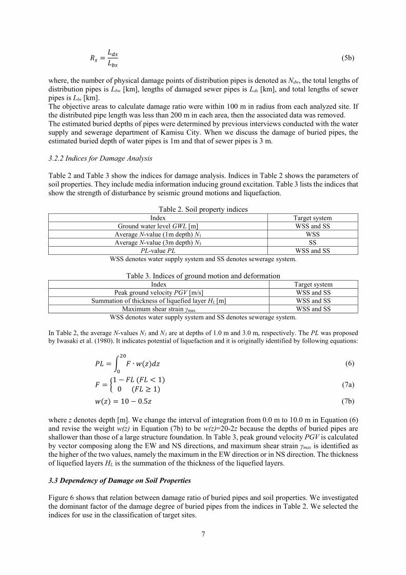
where, the number of physical damage points of distribution pipes is denoted as Ndw, the total lengths of distribution pipes is Lbw [km], lengths of damaged sewer pipes is Lds [km], and total lengths of sewer pipes is Lbs [km]. The objective areas to calculate damage ratio were within 100 m in radius from each analyzed site. If the distributed pipe length was less than 200 m in each area, then the associated data was removed. The estimated buried depths of pipes were determined by previous interviews conducted with the water supply and sewerage department of Kamisu City. When we discuss the damage of buried pipes, the estimated buried depth of water pipes is 1m and that of sewer pipes is 3 m. 3.2.2 Indices for Damage Analysis Table 2 and Table 3 show the indices for damage analysis. Indices in Table 2 shows the parameters of soil properties. They include media information inducing ground excitation. Table 3 lists the indices that show the strength of disturbance by seismic ground motions and liquefaction.
Table 2. Soil property indices Index Target system
Ground water level GWL [m] WSS and SS Average N-value (1m depth) N1 WSS Average N-value (3m depth) N3 SS
PL-value PL WSS and SS WSS denotes water supply system and SS denotes sewerage system.
Table 3. Indices of ground motion and deformation
Index Target system Peak ground velocity PGV [m/s] WSS and SS
Summation of thickness of liquefied layer HL [m] WSS and SS Maximum shear strain γmax WSS and SS
WSS denotes water supply system and SS denotes sewerage system. In Table 2, the average N-values N1 and N3 are at depths of 1.0 m and 3.0 m, respectively. The PL was proposed by Iwasaki et al. (1980). It indicates potential of liquefaction and it is originally identified by following equations:
∙ (6)
1 10 1 (7a)
10 0.5 (7b)
where z denotes depth [m]. We change the interval of integration from 0.0 m to 10.0 m in Equation (6) and revise the weight w(z) in Equation (7b) to be w(z)=20-2z because the depths of buried pipes are shallower than those of a large structure foundation. In Table 3, peak ground velocity PGV is calculated by vector composing along the EW and NS directions, and maximum shear strain γmax is identified as the higher of the two values, namely the maximum in the EW direction or in NS direction. The thickness of liquefied layers HL is the summation of the thickness of the liquefied layers. 3.3 Dependency of Damage on Soil Properties Figure 6 shows that relation between damage ratio of buried pipes and soil properties. We investigated the dominant factor of the damage degree of buried pipes from the indices in Table 2. We selected the indices for use in the classification of target sites.
8
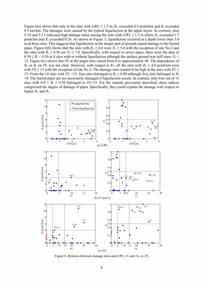
Figure 6(a) shows that only at the sites with GWL ≤ 1.5 m, Rw exceeded 4.0 point/km and Rs exceeded 0.5 km/km. The damages were caused by the typical liquefaction in the upper layers. In contrast, sites 5-10 and 5-13 indicated high damage ratios among the sites with GWL ≥ 1.5 m where Rw exceeded 1.7 point/km and Rs exceeded 0.28. As shown in Figure 5, liquefaction occurred at a depth lower than 3.0 m at these sites. This suggests that liquefaction in the deeper part of ground caused damage to the buried pipes. Figure 6(b) shows that the sites with Rw ≥ 4.0 were N1 ≤ 5.0 with the exception of site No.2 and the sites with Rs ≥ 0.50 are N3 ≤ 7.0. Specifically, with respect to sewer pipes, there were the data of 0.30 ≤ Rs < 0.50 at 8 sites with or without liquefaction although the surface ground was stiff since N3 > 12. Figure 6(c) shows that PL at the target sites varied from 0 to approximately 40. The dependence of Rw or Rs on PL was not clear. However, with respect to Rw, all the sites with Rw ≥ 4.0 point/km were with PL ≥ 15 with the exception of site No.2. The damage ratio tended to be high at the sites with PL ≥ 15. From the 14 sites with PL >15, four sites belonged to Rs ≥ 0.80 although five sites belonged to Rs =0. The buried pipes are not necessarily damaged if liquefaction occurs. In contrast, only four out of 15 sites with 0.0 < Rs ≤ 0.50 belonged to PL>15. For the reasons previously described, these indices categorized the degree of damage of pipes. Specifically, they could explain the damage with respect to higher Rw and Rs.
Figure 6. Relation between damage ratio and GWL, N1 and N3, or PL
(a) GWL
(b) N1 and N3
(c) PL
Rw[p
oint
/km
]
0 1 2 3 40
2
4
6
8
10
12
GWL[m]
5-135-10
Liquefied site
Non-liquefied site
0 5 10 15 200
2
4
6
8
10
12
Rw[p
oint
/km
]
N1
Rs
0 1 2 3 40
0.2
0.4
0.6
0.8
1
GWL[m]
5-10
5-13
0 10 20 30 400
0.2
0.4
0.6
0.8
1
N3
Rs
0 10 20 30 400
0.2
0.4
0.6
0.8
1
Rs
PL
2-2
2-1
0 10 20 30 400
2
4
6
8
10
12
Rw[p
oint
/km
]
PL
2-2
2-1
3-14No.2
5 15 5 15
0.5
0.5
0.5
No.2 2-3
2-61-2
No.2
7
5-105-13
5-14No.1
5-4
12
1-7

9
3.4 Dependence of Damage on Ground Motions and Ground Deformation Figure 7 shows the relation between the damage ratio of buried pipes and ground motion intensity or ground deformation. We investigated the factor of the damage degree of buried pipes with the indices listed in Table 3.
Figure 7. Relation between damage ratio and PGV, HL, and γmax
In Figure 7(a), with respect to the sites with Rw ≤ 4.0 point/km, Rw began to increase from PGV = 0.35 m/s. However, the range of PGV at the four sites with Rw ≥ 4.0 point/km was 0.36 m/s ≤ PGV ≤ 0.47 m/s; and this was considered as wide range. In terms of the relation between PGV and Rs, Rs increased with increases in PGV in the range since PGV > 0.35 m/s. Figure 7(b) shows that the sites with HL ≥ 2.0 m suffered pipe damage in both the water supply and sewerage systems. Given the sites with HL ≥ 2.0 m, the sites with higher Rw or Rs, such as site 2-1, 2-2, and 3-14, were liquefied from the upper to the lower layers. Conversely, the sites with HL < 2.0 m were liquefied only at the upper layers and were severely damaged. When compared with these, the sites only liquefied at the lower layers were included the damage range as Rw < 4.0 point/km or Rs < 0.5. This result implied that the liquefaction at the layers with buried pipes caused damage and that it might be difficult for liquefaction at lower layers to cause
0.30 0.35 0.40 0.45 0.500
2
4
6
8
10
12
(b) HL
HL[m]
Rs
0 2 4 6 8 100
0.2
0.4
0.6
0.8
1
(c) γmax
γmax
Rw[p
oint
/km
]
γmax
Rs
(a) PGVPGV[m/s]
Rw[p
oint
/km
]
Liquefied site
Non-liquefied site
2-2
2-1
3-14
No.2
PGV[m/s]
HL[m]
Rw[p
oint
/km
]
0 2 4 6 8 100
2
4
6
8
10
12R
s
0.30 0.35 0.40 0.45 0.500
0.2
0.4
0.6
0.8
1
0.5
2-2
2-1
No.22-3
2-61-2
0
2
4
6
8
10
122-2
2-1
3-14No.2
10-4 10-3 10-2 10-1 100
1
0
0.2
0.4
0.6
0.8
2-2
2-1
No.2 2-3
2-61-2
10-4 10-3 10-2 10-1 100
0.5
0.5
2-2
2-1
3-14No.2
2-2 2-3
2-6 1-2
2-1
5-11 5-13 2-31-75-101-2
2-41-4 5-13
4-3
1-3
2-5
5-10
No.2

10
the pipe damage from a depth of 1 m to 3 m. Furthermore, high HL caused the damage of buried pipes. However, at the sites with high HL, the ground motions reached a certain of the limit value and the damage by the ground motion was saturated. As a result, the depth of the liquefied layer is a better factor of Rw and Rs when compared to HL. Figure 7(c) shows that Rw increased with increases in γmax at the sites with Rw ≥ 4.0 point/km while the sites with Rw < 4.0 point/km exhibited the scattering of γmax. The liquefaction occurred in the upper layers at the former sites in contrast to the liquefaction of lower layers at the latter sites. When compared with Rw, Rs remained stable with increases in γmax although the values were high. The results suggested that the ground deformation by liquefaction in upper layers could directly cause pipe damage and that the liquefaction in lower layers could also cause the half degree of damage. 4. MODIFICATION OF PREVIOUS FRAGILITY CURVES First, we classified the actual data on damage ratios Rw and Rs at the target sites into two categories according to the PL-values described in the previous chapter, which threshold value is set as PL = 15. Second, we modeled the fragility curves describing the estimating value of damage ratios Rw and Rs by statistically analyzing the actual damage ratio data based on the cumulative distribution function of the log-normal distribution as shown in Equation (8) as follows:
Φln
(8)
where Φ denotes the standard normal cumulative distribution function; C, λ, and ζ denote model parameters determined by using least square method minimizing objective function εm as described in the following equation. Now, C denotes the asymptotic value describing the limit of estimated damage ratio, λ and ζ are the expected value and the standard deviation of logarithmic value of PGV.
(9)
where j denotes the number of classes of PGV in a 3 cm/s unit; nPGV denotes the total number of PGV classes; RX denotes the actual damage ratio Rw or Rs; and Lj denotes the length of exposed pipes for the j-th class in a 3 cm/s unit.
(a) Water pipes (b) Sewer pipes
Figure 8. Relation between the damage ratio and PGV As shown in Figure 8, the PL ≥ 15 group exhibited a lower PGV when compared to that of the PL < 15 group. When the threshold value was set as PL=15, it was effective to examine the difference of the pipe damage due to the ground conditions. Figure 8(a) shows that PGV and Rw were basically related to positive correlation for PL < 15 in the range of PGV ≥ 0.35 m/s. The three points with the highest Rw
Rw
[poi
nt/k
m]
Rs
PGV [m/s] PGV [m/s]
Liquefied site (PL≥15)Liquefied site (PL<15)Non-liquefied site (PL≥15)Non-liquefied site (PL<15)
0.3 0.35 0.4 0.45 0.50
2
4
6
8
10
12
0.3 0.35 0.4 0.45 0.50
0.2
0.4
0.6
0.8
1
0.5

11
were in the group of PL ≥ 15. Figure 8(b) shows that five sites were in the PL ≥ 15 group and only one site was in the PL < 15 group given the sites with Rs > 0.5.
(a) Water pipes (b) Sewer pipes
Figure 9. Data of damage ratio and fragility curves
Figure 9 shows the fragility curves with the threshold value corresponding to PL = 15. The effective range is denoted by solid lines. The result suggests that it is possible to underestimate the damage ratio with a fragility curve that does not include the PL-value information. The fragility curves of both of two groups increase more sharply than those in all sites. 5. CONCLUSIONS This study examined the dependence of damage of buried pipes on strong motion data in the 2011 Tohoku earthquake obtained for liquefied and non-liquefied grounds. The relations between the damage ratio and the ground motion intensities were classified by the soil properties. The modeling of fragility curves were also attempted with respect to the PGV and PL-values. The results are summarized as follows: 1) The numerical results from the one-dimensional effective stress analysis for 39 soil profiles at Kamisu City in Ibaraki Prefecture, Japan were in agreement with actual liquefaction and evaluation by using the FL-value. Liquefaction was observed mostly at lower layers in the analysis. However, it was not actually observed at the sites in which only the lower layers were liquefied 2) By observing the relations between Rw or Rs and GWL, N1, N3, or PL, these indices categorized the degree of damage of pipes with a few threshold values and they could explain the damage for higher Rw and Rs values. 3) From the relations between Rw or Rs and PGV, HL or γmax, PGV showed basically the positive correlation in a certain range. With respect to the sites with high HL, the ground motions reached the limit value and the damage by the ground motion were saturated. The results suggest that the depth of liquefied layer is a better factor when compared to HL. The results of γmax suggest that the ground deformation by liquefaction in upper layers directly causes pipe damage and the liquefaction in lower layers also causes the half degree of damage. 4) The fragility curves were modeled by classifying target sites based on PL-value considering ground conditions. The damage ratio of the sites with PL ≥ 15 rose at approximately a 0.10 m/s lower PGV when compared with that for PL < 15. The result suggests that it is possible to underestimate the damage ratio with the fragility curve that does not include the PL-value information. 6. ACKNOWLEDGMENTS The authors greatly appreciate the thoughtful comments and suggestions by Liquefaction Countermeasure Committee in Kamisu City (Chairperson: Professor Susumu Yasuda at Tokyo Denki University) and all the associated members in the committee. In this study, we would like to deeply appreciate the use of strong motion records offered by National Research Institute for Earth Science and
0 0.1 0.2 0.3 0.4 0.5 0.60
2
4
6
8
10
12
0 0.1 0.2 0.3 0.4 0.5 0.60
0.2
0.4
0.6
0.8
1
Rw
[poi
nt/k
m]
Rs
PGV [m/s] PGV [m/s]
PL≥15
PL<15
All sites
PL≥15
PL<15
All sites

12
Disaster Resilience. 7. REFERENCES The Water Supply Division, Health Service Bureau, Ministry of Health, Labour and Welfare (MHLW). 2013. Final report of Damage of water facilities due to Great East Japan Earthquake, March 2013 (In Japanese) http://www.mhlw.go.jp/topics/bukyoku/kenkou/suido/houkoku/suidou/130801-1.html (accessed 2018.3.5).
Sewerage Technological Examination Committee for Earthquake and Tsunami. Final report, March 2016 (In Japanese) http://www.mlit.go.jp/mizukokudo/sewerage/crd_sewerage_tk_000170-1.html (accessed 2018.3.5).
Hwang, HMH, Lin, H, Shinozuka, M (1998). Seismic performance assessment of water delivery systems. Journal of Infrastructure Systems, 4(3): 118-125.
Liu, GY, Hung, HY (2009). Seismic performance simulation of water systems considering uncertainties in ground motions and pipeline damages. Safety, Reliability and Risk of Structures, Infrastructures and Engineering Systems, Taylor & Francis, London: 2316-2321.
Javanbarg, MB, Takada, S (2009). Seismic reliability assessment of water supply systems. Safety, Reliability and Risk of Structures, Infrastructures and Engineering Systems, Taylor & Francis, London: 3455-3462.
Shoji, G, Naba, S, Nagata, S (2011). Evaluation of Seismic Vulnerability of Sewerage Pipelines based on Assessment of the damage data in the 1995 Kobe Earthquake, Applications of Statistics and Probability in Civil Engineering eds by M. H. Faber, J. Kőhler and K. Nishijima, Taylor & Francis, London: 1415-1423.
Naba, S, Tsukiji, T, Shoji, G, Nagata, S (2012). Damage assessment on water supply system and sewerage system at the 2011 off the Pacific Coast of Tohoku Earthquake -Case study for the data at Ibaraki and Chiba prefectures-. Proceedings of the International Symposium on Engineering Lessons Learned from the 2011 Great East Japan Earthquake, Tokyo, 1-4 March 2012, pp 1487-1495.
Toprak, S, Nacaroglu, E, Koc, AC, van Ballegooy, S, Jacka, M, Torvelainen, E, O’Rourke, TD (2017). Pipeline damage predictions in liquefaction zone using LNS. Proceeding 16th World Conference on Earthquake, 16WCEE 2017, Santiago Chile, 9-13 January 2017, Paper N° 4533.
Tsukiji, T and Shoji, G (2013). Development of Damage Functions on Water Supply Systems subjected to an Extreme Ground Motion, Proceedings of the 11th International Conference on Structural Safety and Reliability (ICOSSAR2013), New York, USA, Safety, Reliability, Risk and Life-Cycle Performance of Structures & Infrastructures eds by G. Deodatis, B. R. Ellingwood and D. M. Frangopol, CRC Press Taylor & Francis, London, pp 691-698.
Unjoh, S, Kaneko, M, Kataoka, S, Nagaya, K, Matsuoka, K (2013). Effect of earthquake ground motions on soil liquefaction. Soils and Foundations, 52(5):830-841.
Yoshida, N, Towhata, I (1991). YUSAYUSA-2 and SIMMDL-2, Theory and Practice, revised in 2003 (Version 2.10) http://www.kiso.co.jp/yoshida/ (accessed 2018.3.5).
The Kanto District Bureau of Ministry of Land, Infrastructure, Transport and Tourism (MILT) (2011). Survey Results of Soil Liquefaction in Kanto region at the 2011 off the Pacific Coast of Tohoku earthquake and tsunami. (In Japanese) http://www.ktr.mlit.go.jp/ktr_content/content/000043569.pdf (accessed 2018.3.5).
Japan Road Association (JRA) (2012). Bridge Design Specifications, Part V Seismic Design (In Japanese).
Hatanaka, M, Uchida, A (1996). Empirical correlation between penetration resistance and internal friction angle for sandy soils, Soils and Foundations, 36(4): 1-9.
Creager, WP, Justin, JD, Hinds, J (1945). Engineering for Dams, Vol. III, Earth, Rock-fill, Steel and Timber dams, John Wiley & Sons, Inc., N.Y., pp 645-649.
Ishihara, K, Towhata, I (1980). One-Dimensional Soil Response Analysis during Earthquakes Based on Effective Stress Method, Journal of Faculty of Engineering, XXXV(4): 655-700.
National Research Institute for Earth Science and Disaster Prevention (NIED) 2011. K-NET and KiK-net. (In Japanese) http://www.kyoshin.bosai.go.jp/kyoshin/ (accessed 2018.3.5).
Yoshida N, Suetomi I (1996). DYNEQ: a computer program for dynamic analysis of level ground based on equivalent linear method. Reports of Engineering Research Institute, Sato Kogyo Co., Ltd, pp 61-70 (In Japanese).

13
Architectural Institute of Japan (1988). Recommendations foe Design of Building Foundations, pp.163-169 (In Japanese).
Iwasaki, T, Tatsuoka, H, Tokida, K, Yasuda, S (1980). Estimation of degree of soil liquefaction during earthquake. Soils and Foundations (Tsuchi-to-Kiso), 28(4): 23-29 (In Japanese).
Japan Meteorological Agency (JMA) (2011). Data of seismic intensity by local public organization. http://www.data.jma.go.jp/svd/eqev/data/kyoshin/jishin/110311_tohokuchiho-taiheiyouoki/index2.html (accessed 2018.3.5).
Sakurai, T, Shoji, G, Takahashi, K, Nakamura, T (2012). Damage assessment on road structures due to slope failures in the 2011 off the Pacific Coast of Tohoku earthquake. Proceedings of the International Symposium on Engineering Lessons Learned from the 2011 Great East Japan Earthquake, Tokyo, 1-4 March 2012, pp 961-972.