Danehy Park Wind Turbine Project Preliminary Assessment Report

Danehy Park Project Group Wind Energy Projects in Action (WEPA) Massachusetts Institute of Technology Cy Chan Project Lead, Resource Assessment, Financial Assessment

Pamela Silva Community and Environmental Assessment

Chao Zhang Financial Assessment

Prepared for the City of Cambridge Spring/Summer 2011 (rev. July 27, 2011)

Acknowledgements

We would like to thank everyone who helped us with this report, including but not limited to:

John Bolduc, Steve Lenkauskas, George Fernandes, and the staff at the City of Cambridge and Danehy

Park who helped shape this report and made on-site instrument installation and data collection possible.

Mark Lipson, Jack Clarke and Jean Rogers for their guidance with the environmental and community

impact assessment.

Bob Paine and Scott Abbett for their thoughts and experiences with the Medford McGlynn School wind

turbine.

Katherine Dykes and Sungho Lee for their leadership, guidance, and feedback.

1

Introduction

This preliminary assessment report investigates the wind resource available at Danehy Park in the City

of Cambridge, providing estimated power generation figures as well as cost and revenue estimates and

potential impacts to wildlife and the surrounding community. A satellite photo of Danehy Park can be

seen in Figure 1.

Figure 1: Danehy Park satellite photo (courtesy of Google Maps). The location of the

light pole where the wind sensors were mounted is marked with a yellow star.

2

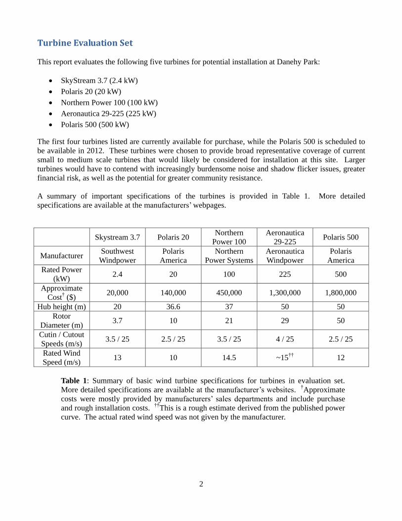
Turbine Evaluation Set

This report evaluates the following five turbines for potential installation at Danehy Park:

SkyStream 3.7 (2.4 kW)

Polaris 20 (20 kW)

Northern Power 100 (100 kW)

Aeronautica 29-225 (225 kW)

Polaris 500 (500 kW)

The first four turbines listed are currently available for purchase, while the Polaris 500 is scheduled to

be available in 2012. These turbines were chosen to provide broad representative coverage of current

small to medium scale turbines that would likely be considered for installation at this site. Larger

turbines would have to contend with increasingly burdensome noise and shadow flicker issues, greater

financial risk, as well as the potential for greater community resistance.

A summary of important specifications of the turbines is provided in Table 1. More detailed

specifications are available at the manufacturers’ webpages.

Skystream 3.7 Polaris 20 Northern

Power 100

Aeronautica

29-225 Polaris 500

Manufacturer Southwest

Windpower

Polaris

America

Northern

Power Systems

Aeronautica

Windpower

Polaris

America

Rated Power

(kW) 2.4 20 100 225 500

Approximate

Cost† ($)

20,000 140,000 450,000 1,300,000 1,800,000

Hub height (m) 20 36.6 37 50 50

Rotor

Diameter (m) 3.7 10 21 29 50

Cutin / Cutout

Speeds (m/s) 3.5 / 25 2.5 / 25 3.5 / 25 4 / 25 2.5 / 25

Rated Wind

Speed (m/s) 13 10 14.5 ~15

†† 12

Table 1: Summary of basic wind turbine specifications for turbines in evaluation set.

More detailed specifications are available at the manufacturer’s websites. †Approximate

costs were mostly provided by manufacturers’ sales departments and include purchase

and rough installation costs. ††

This is a rough estimate derived from the published power

curve. The actual rated wind speed was not given by the manufacturer.

3

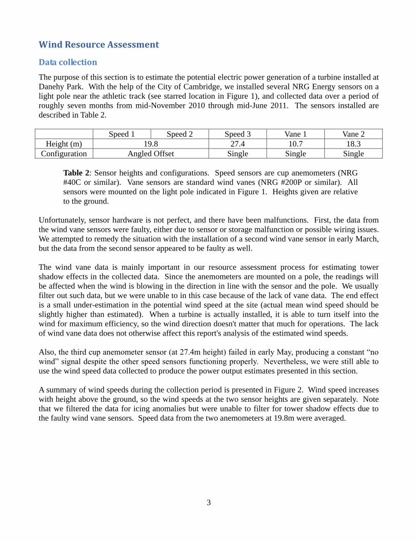
Wind Resource Assessment

Data collection

The purpose of this section is to estimate the potential electric power generation of a turbine installed at

Danehy Park. With the help of the City of Cambridge, we installed several NRG Energy sensors on a

light pole near the athletic track (see starred location in Figure 1), and collected data over a period of

roughly seven months from mid-November 2010 through mid-June 2011. The sensors installed are

described in Table 2.

Speed 1 Speed 2 Speed 3 Vane 1 Vane 2

Height (m) 19.8 27.4 10.7 18.3

Configuration Angled Offset Single Single Single

Table 2: Sensor heights and configurations. Speed sensors are cup anemometers (NRG

#40C or similar). Vane sensors are standard wind vanes (NRG #200P or similar). All

sensors were mounted on the light pole indicated in Figure 1. Heights given are relative

to the ground.

Unfortunately, sensor hardware is not perfect, and there have been malfunctions. First, the data from

the wind vane sensors were faulty, either due to sensor or storage malfunction or possible wiring issues.

We attempted to remedy the situation with the installation of a second wind vane sensor in early March,

but the data from the second sensor appeared to be faulty as well.

The wind vane data is mainly important in our resource assessment process for estimating tower

shadow effects in the collected data. Since the anemometers are mounted on a pole, the readings will

be affected when the wind is blowing in the direction in line with the sensor and the pole. We usually

filter out such data, but we were unable to in this case because of the lack of vane data. The end effect

is a small under-estimation in the potential wind speed at the site (actual mean wind speed should be

slightly higher than estimated). When a turbine is actually installed, it is able to turn itself into the

wind for maximum efficiency, so the wind direction doesn't matter that much for operations. The lack

of wind vane data does not otherwise affect this report's analysis of the estimated wind speeds.

Also, the third cup anemometer sensor (at 27.4m height) failed in early May, producing a constant “no

wind” signal despite the other speed sensors functioning properly. Nevertheless, we were still able to

use the wind speed data collected to produce the power output estimates presented in this section.

A summary of wind speeds during the collection period is presented in Figure 2. Wind speed increases

with height above the ground, so the wind speeds at the two sensor heights are given separately. Note

that we filtered the data for icing anomalies but were unable to filter for tower shadow effects due to

the faulty wind vane sensors. Speed data from the two anemometers at 19.8m were averaged.

4

Figure 2: Measured mean wind speeds at the two sensor heights during the test period.

No wind speed data at 27.4m were available in May or June due to a faulty anemometer.

Figure 3 shows the wind speed distributions measured at each sensor height. Mean and standard

deviation of the wind speeds are given, in addition to the Weibull scale and shape parameters of the

best fit Weibull distribution.

0 5 10 150

0.05

0.1

0.15

0.2

0.25

Danehy Wind Speed at 19.8mMean = 3.9, StDev = 2.0, Scale = 4.4, Shape = 2.0

Wind Speed (m/s)

Pro

ba

bility

0 5 10 150

0.05

0.1

0.15

0.2

0.25

Danehy Wind Speed at 27.4mMean = 4.2, StDev = 2.2, Scale = 4.8, Shape = 2.1

Wind Speed (m/s)

Pro

ba

bility

Figure 3: Histogram of wind speeds measured at the Danehy wind pole over the test

period (mid-November to mid-June). The best-fit Weibull distribution is shown in red.

Means, standard deviations, and best-fit Weibull scale and shape parameters are given.

5

The Weibull distribution is a family of probability distributions commonly used within the wind

industry. Similar to the way a normal distribution describes how the heights or weights of people vary

over a population, the Weibull distribution describes how the wind speed at a particular location varies

over time. The higher the probability value at a certain wind speed, the more likely the wind will be at

around that speed.

The best fit Weibull distribution is the member of the distribution family that best fits the observed data

(i.e. the red curve that most closely fits the blue bars in Figure 3). Calculating the parameters of best fit

allows one to characterize the wind's behavior with only two numbers, the Weibull scale and shape

parameters, which respectively encapsulate the wind's strength and variability. These figures are

included here mainly for the benefit of those who are more knowledgeable about wind resource

assessment.

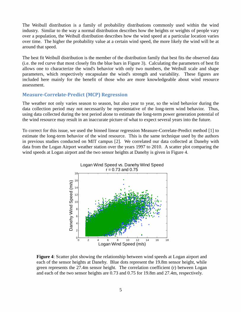
Measure-Correlate-Predict (MCP) Regression

The weather not only varies season to season, but also year to year, so the wind behavior during the

data collection period may not necessarily be representative of the long-term wind behavior. Thus,

using data collected during the test period alone to estimate the long-term power generation potential of

the wind resource may result in an inaccurate picture of what to expect several years into the future.

To correct for this issue, we used the binned linear regression Measure-Correlate-Predict method [1] to

estimate the long-term behavior of the wind resource. This is the same technique used by the authors

in previous studies conducted on MIT campus [2]. We correlated our data collected at Danehy with

data from the Logan Airport weather station over the years 1997 to 2010. A scatter plot comparing the

wind speeds at Logan airport and the two sensor heights at Danehy is given in Figure 4.

0 2 4 6 8 10 12 14 16 180

2

4

6

8

10

12

14

16

18

Logan Wind Speed (m/s)

Da

ne

hy W

ind

Sp

ee

d (

m/s

)

Logan Wind Speed vs. Danehy Wind Speedr = 0.73 and 0.75

Figure 4: Scatter plot showing the relationship between wind speeds at Logan airport and

each of the sensor heights at Danehy. Blue dots represent the 19.8m sensor height, while

green represents the 27.4m sensor height. The correlation coefficient (r) between Logan

and each of the two sensor heights are 0.73 and 0.75 for 19.8m and 27.4m, respectively.

6

The correlation coefficient between wind speeds at Logan and Danehy is approximately 0.74. While

the correlation isn’t perfect, it indicates a strong linear relationship, which gives us the confidence to

proceed with the MCP regression.

After application of the MCP regression technique, we developed a synthetic wind speed profile for the

Danehy site over the 1997 to 2010 historical period. A summary of the resulting estimated long-term

wind behavior for the Danehy Park test site is given in Table 3. Figure 5 shows the estimated long-term

seasonal variation of the site.

Mean Wind Speed

(m/s)

Weibull Scale

Parameter

Weibull Shape

Parameter

Height 1 (19.8 m) 3.6 4.0 1.9

Height 2 (27.4 m) 4.0 4.4 2.0

Table 3: Estimated long-term wind speed characteristics at the sensor heights.

Figure 5: Estimated long-term seasonal behavior of the mean wind speed at each sensor

height at Danehy Park.

7

Power Calculations

Since wind speed increases with height, we must calculate estimated wind speeds at the height of the

turbine hub for each of the turbines in our evaluation set in order to compute estimated power

generation. The equation governing the relationship between wind speed and height is the wind shear

equation:

,

where v0 is the speed at some reference height h0, and v is the speed to be calculated at the desired

height h [3]. The wind shear exponent a governs how the speed increases with height and depends on

the surface roughness at the location in question. A higher wind shear exponent corresponds to a more

pronounced variation in wind speed for the same change in height. A table of common wind shear

exponents for various surface roughness conditions is given in [3].

Given the wind speeds measured at the two sensor heights at Danehy, we computed the approximate

wind shear exponent for our site to be 0.28. This corresponds roughly with the value given in [3] for

unstable air above human inhabited areas.

Table 4 shows the estimated annual electrical energy generation potential of each of the turbines in our

evaluation set using our estimated wind speeds scaled to hub height using a wind shear exponent of

0.28. Manufacturer provided power curves were used to convert wind speed to power generation.

Skystream

3.7 Polaris 20

Northern Power

100

Aeronautica

29-225 Polaris 500

Hub Height (m) 20 36.6 37 50 50

Est. Mean Wind Speed

at Hub Height (m/s) 3.7 4.4 4.4 4.8 4.8

Annual Energy

Production (kWh) 1,500 19,100 104,100 233,400 744,900

Table 4: Estimated Annual Energy Production for each turbine in our evaluation set. Hub

height and estimated mean wind speed at hub height for each turbine are also given.

In the next section, we will discuss the estimated financial value of the power produced for each of the

turbine cases.

References

[1] A Rogers, J Rogers, J Manwell, “Review of Measure-Correlate-Predict Algorithms and Comparison

of the Performance of Four Approaches,” Journal of Wind Engineering and Industrial Aerodynamics,

93:3, pp. 243-264, 2005.

[2] K Araujo, K Dykes, C Chan, A Kalmikov, K Ferrigno, B Palmintier, S Lee, M Lipson, "Feasibility

Study – Project Full Breeze", Project Report Submitted to MIT Facilities, 2010.

[3] M Kaltschmitt, W Streicher, A Wiese, Renewable energy: technology, economics, and environment,

p. 55, Springer, 2007.

8

Financial Assessment

In this section, we examine each of the turbines in our evaluation set to determine the value of a turbine

installation. Table 5 lists a summary of important financial data for each turbine.

Skystream

3.7 Polaris 20

Northern

Power 100

Aeronautica

29-225 Polaris 500

Rated Power (kW) 2.4 20 100 225 500

Approximate

Purchase Cost† ($)

17,000 80,000 350,000 400,000 1,200,000

Approximate

Installation Cost† ($)

3,000 60,000 100,000 900,000 600,000

Estimated Annual

Energy Production (kWh) 1,500 19,100 104,100 233,400 744,900

Value of Electricity

in First Year ($) 220 2,900 15,600 35,000 111,700

Estimated NPV

at 25 Years††

($) -17,500 -105,600 -261,400 -877,200 -418,900

Production Incentive

Required for $0 NPV

at 25 Years ($ / kWh)

1.09 0.51 0.23 0.34 0.05

Table 5: Summary of financial data for each turbine in our evaluation set. †Approximate

costs are mostly provided by manufacturers’ sales departments and should be considered

rough. ††

The calculated NPVs shown do NOT include any incentives or grants, only

the approximate costs of purchase, installation, O&M, and insurance and the direct value

of the electricity generated at $0.15 / kWh.

We were unable to determine which federal and state incentives would be applicable for a turbine

installation at Danehy Park. Most tax incentives we found apply for commercial or residential

installations, so it is not clear what incentives would apply for a municipal installation. A deal with the

commercial developer or utility may be possible where they can claim any applicable tax credits and

pass some of the savings on to the City. Though this preliminary analysis does not include the effect of

incentives, they should be factored into any further studies.

The purchase and installation costs of the turbines were mostly provided by the manufacturers’ sales

departments. In the case of the Northern Power 100, we used the breakdown of costs used by the City

of Medford feasibility study for an installation at the McGlynn and Andrews Middle Schools [1].

For all of the turbines in our set, we used common parameters to determine the approximate operations

and maintenance ($0.015 / kWh) and insurance ($10 / kW) costs. We assumed the value of electricity

generated to be $0.15 / kWh and used a 3% annual escalation in the costs of energy, O&M, and

insurance. We computed net present values (NPVs) assuming an 8% discount rate. Using these

parameters, we computed the cash flow tables given in Appendix A. The resulting NPVs at 25 years

are listed in Table 5 above.

The last row of Table 5 gives the production incentive level ($ / kWh) required in order to reach a

break-even NPV in the 25 year time frame (assuming $0 grants). This figure is provided to give a basic

9

idea of the necessary incentive levels required to make a turbine installation at this site viable. On the

other hand, if no production credits were available, the amount of grants necessary to break even in the

25 year time frame is equal to the negative of the estimated NPV listed in the table. Taking the

Northern Power 100 turbine as an example, either $261,400 in grants or a $0.23 / kWh production

credit would lead to the turbine breaking even in 25 years. Combinations of the two incentive types

would also work (e.g. $130,700 in grants and a $0.115 / kWh production credit) to bring the 25 year

NPV to break-even.

Note that the incentive levels given in Table 5 should be treated as rough estimates since the numbers

they are based on are also rough. We assumed no escalation in production credits when computing

NPVs.

It is important to recognize that there may be other significant costs associated with a turbine

installation that are not covered in this preliminary assessment report. For example, since Danehy Park

is built on capped landfill, there could be extra costs associated with installation, such as cap

penetration and contaminated soil management. While we did not have the resources to address these

issues in this report, further investigation will be required before a turbine installation can proceed.

References

[1] Sustainable Energy Developments, “City of Medford Wind Power Feasibility Study – The McGlynn

and Andrews Middle Schools,” 2006.

10

Environmental Impact Considerations

Resident and Migratory Birds

Danehy Park is located within a mile of Fresh Pond, a large body of water located in West Cambridge,

MA. Mass Audubon, an organization dedicated to the protection of Massachusetts wildlife, has

denominated Fresh Pond as an Important Bird Area of category 3, which indicates that birds

concentrate in significant numbers in breeding season, in winter, or during migration [1]. Many bird

species have been observed in Fresh Pond throughout the years, some frequently and at specific

seasons, and some only occasionally. Some of the infrequently observed species (some seen once or

twice in nine years) are the Black Scoter, Common Goldeneye, Eurasian Wigeon, Green-winged Teal,

Redhead, Common Loon, Gadwall, Wood Duck, American Bittern, and the Pied-billed Grebe. Of these

species, only the Common Loon, the American Bittern, and the Pied-billed Grebe are listed as special

concern or endangered species in Massachusetts [2]. Nevertheless, Fresh Pond is a common habitat and

migratory stopover for other bird species frequently observed at the site, such as the Ring-billed Gull,

Canada Goose, Greater Scaup, Hooded Merganser, Common Merganser, American Coot, American

Wigeon, Canvasback, Ring-necked Duck, Ruddy Duck, Lesser Scaup, Bufflehead, and Mallard [1].

None of these species are endangered species, according to the Massachusetts Division of Fisheries and

Wildlife.

The frequently observed species listed above could potentially be at risk by the placement of a wind

turbine in Danehy Park, a site in the vicinity of Fresh Pond. Populations of some of these species have

been previously observed in sites where wind turbines or wind farms have been placed and behavioral

patterns have been recorded. A Bird Monitoring Program performed in Toronto, Canada, near the

waters of Lake Ontario, reported frequent observations of Ring-billed Gulls near the wind turbine area.

Flocks were seen very frequently flying close to turbine at the height of the blades, and it was observed

that they always took a path that avoided coming close to the turbine [3]. In a similar manner, a study

at the Lely wind farm in the Netherlands, revealed that the Greater Scaup avoided flying close to the

wind farm, even on moonless nights [5].

It has also been reported that Canada Geese have been observed flying within blade distance (40m-

90m) on wind turbines placed in Northeastern Wisconsin, and although it was one of the most frequent

bird species in the area, no collisions with wind turbines were recorded. Similarly, large populations of

the Hooded Merganser and the Common Merganser were recorded in the same site, (for the latter,

flocks were seen flying near the turbine area), and no fatalities were recorded for either species [4].

At a wind farm in Buffalo Ridge, Minnesota, the mortality of one Ruddy Duck was reported in a two-

year period [6], and additionally, one Ring-necked duck carcass was found in a period of five years, in

the Altamont Pass Wind Resources Area, California, an area that includes 5,400 wind turbines[7] . In

surveys of 114 wind turbines at the McBridge Lake Wind Farm in Alberta, Canada, for a one year

period, one Canvasback carcass was recovered[8]. Furthermore, a 15 month study in a San Gorgonio,

California wind farm, which includes 360 turbines, reported six deaths of the American Coot[6].

Bats

Little Brown Bats and Large Brown Bats are common in the Danehy Park area (Jean Rogers, personal

communication). These species are not endangered, and their foraging behavior leads to their low

mortality rates due to wind turbine collisions, even at sites of active populations. [9].

11

References

[1] Mass Audubon (2011). Massachusetts Important Bird Areas; Fresh Pond:

http://www.massaudubon.org/Birds_and_Birding/IBAs/site_summary.php?getsite=46.

[2] Massachusetts Division of Fisheries and Wildlife (2008). Massachusetts List of Endangered,

Threatened and Special Concern Species:

http://www.mass.gov/dfwele/dfw/nhesp/species_info/mesa_list/mesa_list.html.

[3] James, R.D., & Coady, Glenn. (2003). “Exhibition Place Wind Turbine Bird Monitoring Program in

2003”. Report submitted to Windshare and Toronto Hydro Energy Services.

[4] Howe, R.W, Evans, W., & Wolf, A.T. (2002). “Effects of Wind Turbines on Birds and Bats in

Northeastern Wisconsin”. Winsconsin, USA.

[5] Giuarnaccia, J, & Kerlinger, P. (2008). “Avian Risk Assessment”. Report submitted to Great Lakes

Wind Energy Center. Cuyahoga County, Ontario

[6] Erickson , W., Johnson, G., Strickland, M., Young, D., & Sernka, K. , Good R. (2001). “Avian

Collisions with Wind Turbines: a Summary of Existing Studies and Comparisons to other Sources of

Avian Collision Mortality in the United States” National Wind Coordinating Committee. Chayenne,

WY.

[7] Smallwood, K., & Thelander, C. (2008). “Bird Mortality in the Altamont Pass Wind Resource Area,

California.” The Journal of Wildlife Management, 72, 215-223.

[8] Brown, K., & Hamilton, B. (2004). “Bird and Bat Monitoring at the McBride Lake Wind Farm,

Alberta 2003-2004”. Vision Quest Wind Electric Inc. Calgary, AB.

[9] Araujo, K., Dykes, K., Chan, C., Kalmikov, A., Ferrigno, K., Palmintier, B., Lee, S., Lipson, M.,

(2010) "Feasibility Study -- Project Full Breeze", Project report submitted to MIT Facilities.

12

Community Impact – Shadow Flicker Analysis

Overview

The blades of a wind turbine cast moving shadows as they rotate, creating a shadow flicker effect that

may affect residents nearby. This phenomenon occurs when the sun is low in the sky and shines on a

building from behind the turbine rotor and the shadow of the blades is then cast onto the building. As

the turbine rotates, the shadow appears to flick on and off. The shadow flicker of a rotating wind

turbine can be bothersome to eyesight at certain frequencies. The frequencies that produce disturbances

to the general population, as well as the two percent of people who suffer from epilepsy, lie above

2.5Hz. The effect of the shadow flicker reduces non-linearly as a function of distance from the turbine.

Since the effect of the shadow flicker diminishes with distance, at a distance of 10 rotor diameters, it

should not be perceivable, as the turbine is just perceived as an object with the sun behind it. [1]. In

order asses the community impact of placing a wind turbine in Danehy Park, we aim to estimate the

area at which the shadow flicker effect could be perceivable, and its overlap with buildings or

residential areas in the vicinity of the park.

Danehy Park

The shadow created by the wind turbine blades is dependent on the sun trajectory for the specific

location of study. The sun path diagram corresponding to the particular location of Danehy Park in

Cambridge, MA, is given below.

Figure 6: Sun path record for Danehy Park from January– June

13

The calculation of location of shadow flicker can be made by drawing a straight line between the sun,

turbine and ground receptor [2]. The shadow topography, which depends on the height of the turbine

tower, is shown below for the five wind turbines under consideration.

Since the shadow flicker effect is not perceivable at a distance greater than roughly 10 rotor diameters,

the area in which shadow flicker may be a cause of concern is limited to the intersection of the shadow

topography region and a circle of radius 10 rotor diameters around the turbine base. The area of

concern is depicted in park maps in the following sections for each of the turbines under consideration.

SkyStream 3.7

The sun path and shadow topography model for the SkyStream 3.7 wind turbine, with a 20m tower, is

shown below. At a distance of 10 rotor diameters (corresponding to approximately 37m for this turbine

model), the shadow flicker of the rotating turbine blades would not be perceivable. The intersection

between the shadow cast by the turbine, and this specified area is shown interposed in the map of

Danehy Park. As show by the figure, there are several possible turbine placement locations at which the

shadow flicker area would not interfere with buildings or residential areas.

Figure 7: Sun path record for Danehy Park from July – December

14

Figure 8: A computational representation of the Danehy Park sun trajectory and

shadow topography on the ground for the SkyStream 3.7 [3D VIEW]

Figure 9: Expected topography of shadow flicker effect (indicated by blue stripes) over Danehy

Park at various particular wind turbine sites for the SkyStream 3.7.

15

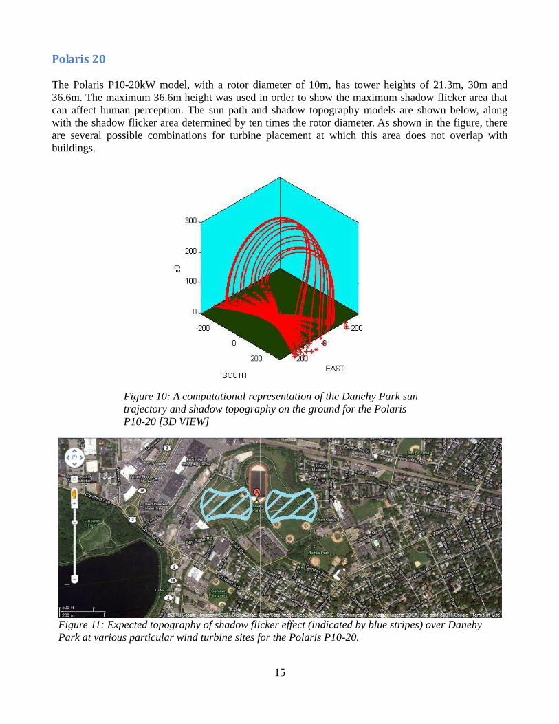
Polaris 20

The Polaris P10-20kW model, with a rotor diameter of 10m, has tower heights of 21.3m, 30m and

36.6m. The maximum 36.6m height was used in order to show the maximum shadow flicker area that

can affect human perception. The sun path and shadow topography models are shown below, along

with the shadow flicker area determined by ten times the rotor diameter. As shown in the figure, there

are several possible combinations for turbine placement at which this area does not overlap with

buildings.

Figure 10: A computational representation of the Danehy Park sun

trajectory and shadow topography on the ground for the Polaris

P10-20 [3D VIEW]

Figure 11: Expected topography of shadow flicker effect (indicated by blue stripes) over Danehy

Park at various particular wind turbine sites for the Polaris P10-20.

16

Northern Power 100

The Northern Power 100 wind turbine, with a rotor diameter of 21m, has a 37m tower. The sun path

and shadow models for the turbine are shown below. Given that the rotor diameter of this wind turbine

is larger than the previously studied ones, the area at which the turbine could be located such that

shadow flicker does not interfere with buildings or residences is more limited.

Figure 12: A computational representation of the Danehy Park sun

trajectory and shadow topography on the ground for the Northern Power

100 [3D VIEW]

Figure 13: Expected topography of shadow flicker effect (indicated by blue stripes) over Danehy Park

at one particular wind turbine site for the Northern Power 100.

17

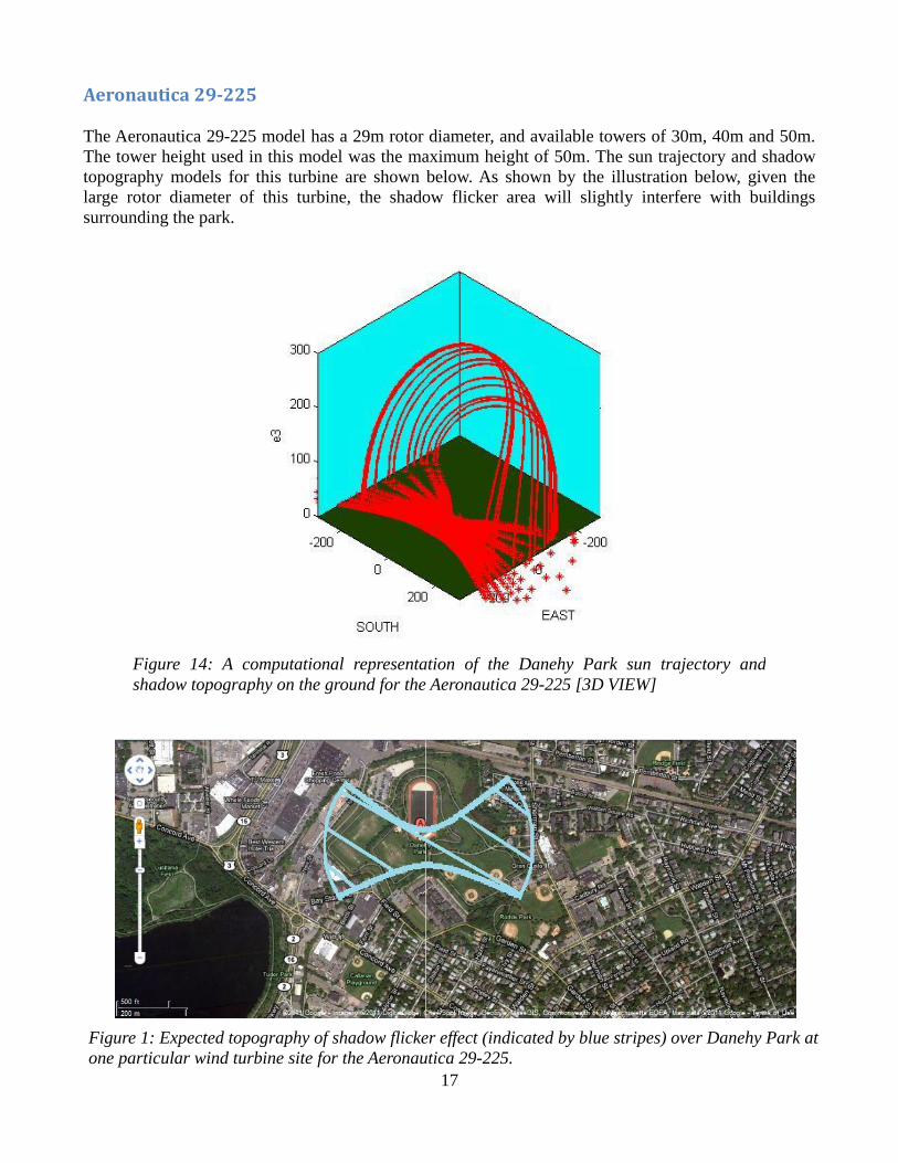
Aeronautica 29-225

The Aeronautica 29-225 model has a 29m rotor diameter, and available towers of 30m, 40m and 50m.

The tower height used in this model was the maximum height of 50m. The sun trajectory and shadow

topography models for this turbine are shown below. As shown by the illustration below, given the

large rotor diameter of this turbine, the shadow flicker area will slightly interfere with buildings

surrounding the park.

Figure 14: A computational representation of the Danehy Park sun trajectory and

shadow topography on the ground for the Aeronautica 29-225 [3D VIEW]

Figure 1: Expected topography of shadow flicker effect (indicated by blue stripes) over Danehy Park at

one particular wind turbine site for the Aeronautica 29-225.

18

Polaris 500

The Polaris P50-500 Wind turbine has a rotor diameter of 50m and tower heights of 50m, 60m, and

70m. The sun path trajectory and shadow model for the 50m tower is shown below. Since the rotor

diameter of this wind turbine is so large, the area within which the shadow flicker effect could be

perceivable would unavoidably interfere with buildings around the park.

Figure 2: A computational representation of the Danehy Park sun trajectory and

shadow topography on the ground for the Polaris P50-500 [3D-VIEW]

Figure 17: Expected topography of shadow flicker effect (indicated by blue stripes) over

Danehy Park at one particular wind turbine site for the Polaris P50-500.

19

As can be seen from the diagrams, shadow flicker effect would likely not be a problem for nearby

residents with the smaller wind turbine models Skystream 3.7, Polaris 20, and Northern Power 100. It

could, however, present an issue for larger wind turbines, such as Aeronautica 29-225 and Polaris 500.

References

[1] UK Department of Business, Innovation and Skills:

http://webarchive.nationalarchives.gov.uk/+/http://www.berr.gov.uk//energy/sources/renewables/planni

ng/onshore-wind/shadow-flicker/page18736.html

[2] Araujo, K., Dykes, K., Chan, C., Kalmikov, A., Ferrigno, K., Palmintier, B., Lee, S., Lipson, M.,

(2010) "Feasibility Study -- Project Full Breeze", Project report submitted to MIT Facilities.

[3] Topography from GoogleEarth.com

20

Community Impact – Noise Analysis

Another issue that is frequently associated with wind turbine development is that of noise impact. Each

wind turbine has a noise level measured in decibels (dB) which decreases as a function of distance

from the nacelle, as shown in the figure below.

Figure 18: Sample sound distribution for a large wind turbine. Note: 300 meter distance limit is for

the example turbine shown and is not applicable to all turbine sizes and locations. Source: GE Global

Research

21

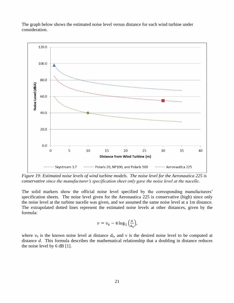
The graph below shows the estimated noise level versus distance for each wind turbine under

consideration.

Figure 19: Estimated noise levels of wind turbine models. The noise level for the Aeronautica 225 is

conservative since the manufacturer’s specification sheet only gave the noise level at the nacelle.

The solid markers show the official noise level specified by the corresponding manufacturers’

specification sheets. The noise level given for the Aeronautica 225 is conservative (high) since only

the noise level at the turbine nacelle was given, and we assumed the same noise level at a 1m distance.

The extrapolated dotted lines represent the estimated noise levels at other distances, given by the

formula:

,

where v0 is the known noise level at distance d0, and v is the desired noise level to be computed at

distance d. This formula describes the mathematical relationship that a doubling in distance reduces

the noise level by 6 dB [1].

22

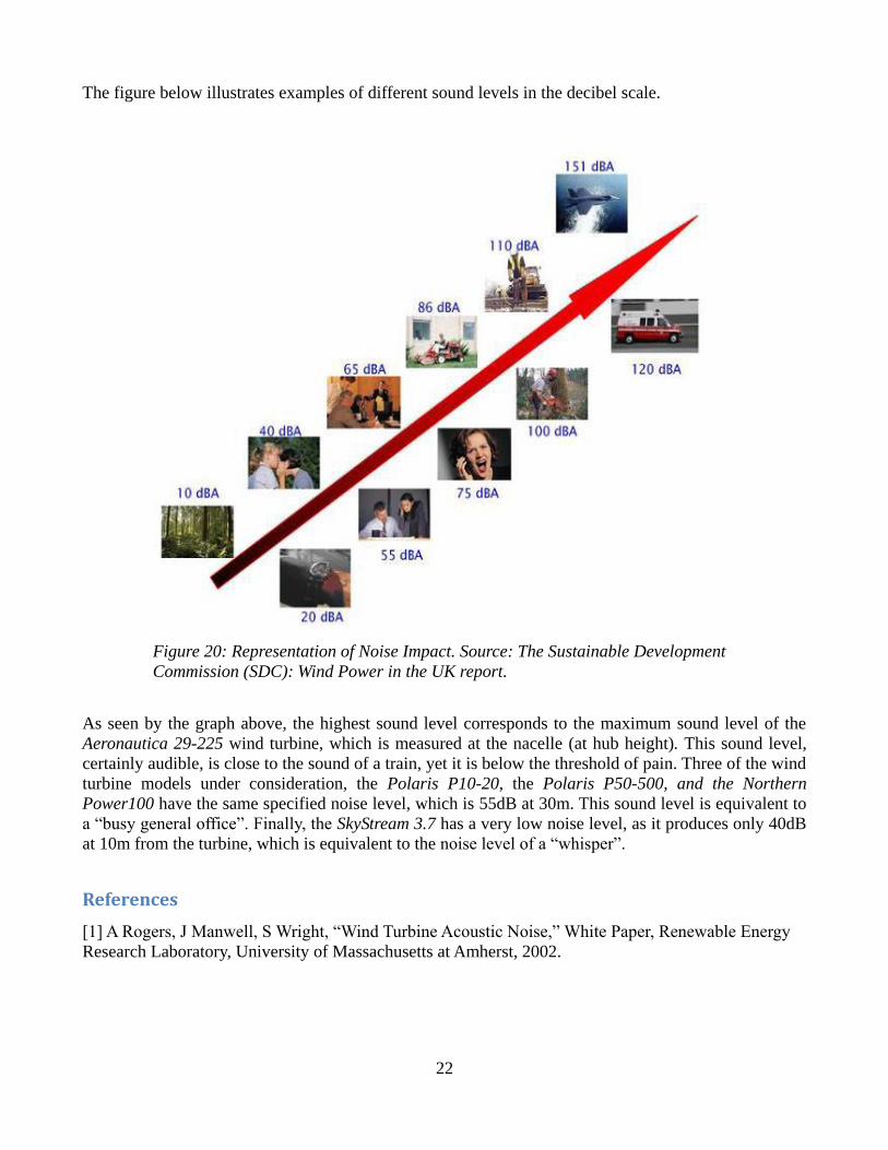
The figure below illustrates examples of different sound levels in the decibel scale.

As seen by the graph above, the highest sound level corresponds to the maximum sound level of the

Aeronautica 29-225 wind turbine, which is measured at the nacelle (at hub height). This sound level,

certainly audible, is close to the sound of a train, yet it is below the threshold of pain. Three of the wind

turbine models under consideration, the Polaris P10-20, the Polaris P50-500, and the Northern

Power100 have the same specified noise level, which is 55dB at 30m. This sound level is equivalent to

a “busy general office”. Finally, the SkyStream 3.7 has a very low noise level, as it produces only 40dB

at 10m from the turbine, which is equivalent to the noise level of a “whisper”.

References

[1] A Rogers, J Manwell, S Wright, “Wind Turbine Acoustic Noise,” White Paper, Renewable Energy

Research Laboratory, University of Massachusetts at Amherst, 2002.

Figure 20: Representation of Noise Impact. Source: The Sustainable Development

Commission (SDC): Wind Power in the UK report.

23

Appendix A – Estimated Cash Flow Tables

For each of the turbines in our evaluation set, we used common parameters to determine the

approximate operations and maintenance ($0.015 / kWh) and insurance ($10 / kW) costs. We assumed

the value of electricity generated to be $0.15 / kWh and used a 3% annual escalation in the costs of

energy, O&M, and insurance. All figures listed in the tables below are net present values (NPVs)

assuming an 8% annual discount rate. Theses tables do NOT include any incentives or grants, only

the approximate costs of purchase, installation, O&M, and insurance and the direct value of the

electricity generated at $0.15 / kWh.

24

SkyStream 3.7

Year

Net

Energy†

O&M Costs Insurance

Annual Cash

Flow†

Total Cash

Flow†

0 ($20,000) ($20,000)

1 $220 ($22) ($24) $174 ($19,826)

2 $209 ($21) ($23) $165 ($19,660)

3 $199 ($20) ($22) $157 ($19,503)

4 $189 ($19) ($21) $149 ($19,354)

5 $179 ($18) ($20) $142 ($19,212)

6 $170 ($17) ($19) $135 ($19,077)

7 $162 ($16) ($18) $128 ($18,949)

8 $154 ($15) ($17) $122 ($18,827)

9 $146 ($15) ($16) $116 ($18,712)

10 $139 ($14) ($15) $110 ($18,602)

11 $132 ($13) ($14) $104 ($18,498)

12 $125 ($13) ($14) $99 ($18,399)

13 $119 ($12) ($13) $94 ($18,305)

14 $113 ($11) ($12) $89 ($18,215)

15 $107 ($11) ($12) $85 ($18,130)

16 $102 ($10) ($11) $81 ($18,050)

17 $97 ($10) ($11) $77 ($17,973)

18 $92 ($9) ($10) $73 ($17,900)

19 $87 ($9) ($10) $69 ($17,831)

20 $83 ($8) ($9) $66 ($17,765)

21 $79 ($8) ($9) $62 ($17,703)

22 $75 ($7) ($8) $59 ($17,643)

23 $71 ($7) ($8) $56 ($17,587)

24 $68 ($7) ($7) $54 ($17,534)

25 $64 ($6) ($7) $51 ($17,483)

26 $61 ($6) ($7) $48 ($17,434)

27 $58 ($6) ($6) $46 ($17,388)

28 $55 ($6) ($6) $44 ($17,345)

29 $52 ($5) ($6) $41 ($17,303)

30 $50 ($5) ($5) $39 ($17,264)

†Figures do not include the effect of any incentives.

25

Polaris 20

Year

Net

Energy†

O&M Costs Insurance

Annual Cash

Flow†

Total Cash

Flow†

0 ($140,000) ($140,000)

1 $2,864 ($286) ($200) $2,378 ($137,622)

2 $2,721 ($272) ($190) $2,259 ($135,364)

3 $2,585 ($258) ($181) $2,146 ($133,218)

4 $2,455 ($246) ($171) $2,038 ($131,180)

5 $2,333 ($233) ($163) $1,937 ($129,243)

6 $2,216 ($222) ($155) $1,840 ($127,403)

7 $2,105 ($211) ($147) $1,748 ($125,656)

8 $2,000 ($200) ($140) $1,660 ($123,995)

9 $1,900 ($190) ($133) $1,577 ($122,418)

10 $1,805 ($181) ($126) $1,498 ($120,920)

11 $1,715 ($171) ($120) $1,424 ($119,496)

12 $1,629 ($163) ($114) $1,352 ($118,144)

13 $1,548 ($155) ($108) $1,285 ($116,859)

14 $1,470 ($147) ($103) $1,220 ($115,638)

15 $1,397 ($140) ($98) $1,159 ($114,479)

16 $1,327 ($133) ($93) $1,102 ($113,377)

17 $1,261 ($126) ($88) $1,046 ($112,331)

18 $1,197 ($120) ($84) $994 ($111,337)

19 $1,138 ($114) ($79) $944 ($110,392)

20 $1,081 ($108) ($75) $897 ($109,495)

21 $1,027 ($103) ($72) $852 ($108,643)

22 $975 ($98) ($68) $810 ($107,833)

23 $927 ($93) ($65) $769 ($107,064)

24 $880 ($88) ($61) $731 ($106,333)

25 $836 ($84) ($58) $694 ($105,639)

26 $794 ($79) ($55) $660 ($104,980)

27 $755 ($75) ($53) $627 ($104,353)

28 $717 ($72) ($50) $595 ($103,758)

29 $681 ($68) ($48) $565 ($103,192)

30 $647 ($65) ($45) $537 ($102,655)

†Figures do not include the effect of any incentives.

26

Northern Power 100

Year

Net

Energy†

O&M Costs Insurance

Annual Cash

Flow†

Total Cash

Flow†

0 ($450,000) ($450,000)

1 $15,609 ($1,561) ($1,000) $13,048 ($436,952)

2 $14,828 ($1,483) ($950) $12,395 ($424,557)

3 $14,087 ($1,409) ($903) $11,776 ($412,781)

4 $13,382 ($1,338) ($857) $11,187 ($401,595)

5 $12,713 ($1,271) ($815) $10,627 ($390,967)

6 $12,078 ($1,208) ($774) $10,096 ($380,871)

7 $11,474 ($1,147) ($735) $9,591 ($371,280)

8 $10,900 ($1,090) ($698) $9,112 ($362,168)

9 $10,355 ($1,036) ($663) $8,656 ($353,512)

10 $9,837 ($984) ($630) $8,223 ($345,289)

11 $9,345 ($935) ($599) $7,812 ($337,477)

12 $8,878 ($888) ($569) $7,422 ($330,055)

13 $8,434 ($843) ($540) $7,050 ($323,005)

14 $8,013 ($801) ($513) $6,698 ($316,307)

15 $7,612 ($761) ($488) $6,363 ($309,944)

16 $7,231 ($723) ($463) $6,045 ($303,899)

17 $6,870 ($687) ($440) $5,743 ($298,156)

18 $6,526 ($653) ($418) $5,456 ($292,701)

19 $6,200 ($620) ($397) $5,183 ($287,518)

20 $5,890 ($589) ($377) $4,924 ($282,594)

21 $5,595 ($560) ($358) $4,677 ($277,917)

22 $5,316 ($532) ($341) $4,444 ($273,473)

23 $5,050 ($505) ($324) $4,221 ($269,252)

24 $4,797 ($480) ($307) $4,010 ($265,242)

25 $4,558 ($456) ($292) $3,810 ($261,432)

26 $4,330 ($433) ($277) $3,619 ($257,813)

27 $4,113 ($411) ($264) $3,438 ($254,374)

28 $3,908 ($391) ($250) $3,266 ($251,108)

29 $3,712 ($371) ($238) $3,103 ($248,005)

30 $3,527 ($353) ($226) $2,948 ($245,057)

†Figures do not include the effect of any incentives.

27

Aeronautica 29-225

Year

Net

Energy†

O&M Costs Insurance

Annual Cash

Flow†

Total Cash

Flow†

0 ($1,300,000) ($1,300,000)

1 $35,005 ($3,501) ($2,250) $29,255 ($1,270,745)

2 $33,255 ($3,325) ($2,138) $27,792 ($1,242,954)

3 $31,592 ($3,159) ($2,031) $26,402 ($1,216,551)

4 $30,012 ($3,001) ($1,929) $25,082 ($1,191,469)

5 $28,512 ($2,851) ($1,833) $23,828 ($1,167,641)

6 $27,086 ($2,709) ($1,741) $22,637 ($1,145,005)

7 $25,732 ($2,573) ($1,654) $21,505 ($1,123,500)

8 $24,445 ($2,445) ($1,571) $20,430 ($1,103,070)

9 $23,223 ($2,322) ($1,493) $19,408 ($1,083,662)

10 $22,062 ($2,206) ($1,418) $18,438 ($1,065,225)

11 $20,959 ($2,096) ($1,347) $17,516 ($1,047,709)

12 $19,911 ($1,991) ($1,280) $16,640 ($1,031,069)

13 $18,915 ($1,892) ($1,216) $15,808 ($1,015,261)

14 $17,970 ($1,797) ($1,155) $15,018 ($1,000,243)

15 $17,071 ($1,707) ($1,097) $14,267 ($985,977)

16 $16,218 ($1,622) ($1,042) $13,553 ($972,423)

17 $15,407 ($1,541) ($990) $12,876 ($959,548)

18 $14,636 ($1,464) ($941) $12,232 ($947,316)

19 $13,905 ($1,390) ($894) $11,620 ($935,695)

20 $13,209 ($1,321) ($849) $11,039 ($924,656)

21 $12,549 ($1,255) ($807) $10,487 ($914,169)

22 $11,921 ($1,192) ($766) $9,963 ($904,206)

23 $11,325 ($1,133) ($728) $9,465 ($894,741)

24 $10,759 ($1,076) ($692) $8,992 ($885,749)

25 $10,221 ($1,022) ($657) $8,542 ($877,207)

26 $9,710 ($971) ($624) $8,115 ($869,092)

27 $9,225 ($922) ($593) $7,709 ($861,383)

28 $8,763 ($876) ($563) $7,324 ($854,059)

29 $8,325 ($833) ($535) $6,958 ($847,102)

30 $7,909 ($791) ($508) $6,610 ($840,492)

†Figures do not include the effect of any incentives.

28

Polaris 500

Year

Net

Energy†

O&M Costs Insurance

Annual Cash

Flow†

Total Cash

Flow†

0 ($1,800,000) ($1,800,000)

1 $111,739 ($11,174) ($5,000) $95,565 ($1,704,435)

2 $106,152 ($10,615) ($4,750) $90,787 ($1,613,648)

3 $100,844 ($10,084) ($4,513) $86,247 ($1,527,401)

4 $95,802 ($9,580) ($4,287) $81,935 ($1,445,466)

5 $91,012 ($9,101) ($4,073) $77,838 ($1,367,627)

6 $86,461 ($8,646) ($3,869) $73,946 ($1,293,681)

7 $82,138 ($8,214) ($3,675) $70,249 ($1,223,432)

8 $78,031 ($7,803) ($3,492) $66,737 ($1,156,695)

9 $74,130 ($7,413) ($3,317) $63,400 ($1,093,296)

10 $70,423 ($7,042) ($3,151) $60,230 ($1,033,066)

11 $66,902 ($6,690) ($2,994) $57,218 ($975,848)

12 $63,557 ($6,356) ($2,844) $54,357 ($921,490)

13 $60,379 ($6,038) ($2,702) $51,640 ($869,851)

14 $57,360 ($5,736) ($2,567) $49,058 ($820,793)

15 $54,492 ($5,449) ($2,438) $46,605 ($774,188)

16 $51,768 ($5,177) ($2,316) $44,274 ($729,914)

17 $49,179 ($4,918) ($2,201) $42,061 ($687,853)

18 $46,720 ($4,672) ($2,091) $39,958 ($647,896)

19 $44,384 ($4,438) ($1,986) $37,960 ($609,936)

20 $42,165 ($4,217) ($1,887) $36,062 ($573,874)

21 $40,057 ($4,006) ($1,792) $34,259 ($539,615)

22 $38,054 ($3,805) ($1,703) $32,546 ($507,070)

23 $36,151 ($3,615) ($1,618) $30,918 ($476,151)

24 $34,344 ($3,434) ($1,537) $29,373 ($446,778)

25 $32,627 ($3,263) ($1,460) $27,904 ($418,875)

26 $30,995 ($3,100) ($1,387) $26,509 ($392,366)

27 $29,445 ($2,945) ($1,318) $25,183 ($367,183)

28 $27,973 ($2,797) ($1,252) $23,924 ($343,258)

29 $26,575 ($2,657) ($1,189) $22,728 ($320,530)

30 $25,246 ($2,525) ($1,130) $21,592 ($298,939)

†Figures do not include the effect of any incentives.