Daniel J. Vimont, Ralf Bennartz Amato Evan Dept of Atmospheric and Oceanic Sciences Department of Environmental Sciences University of Wisconsin – Madison University of Virginia Email: dvimont@wisc.edu Email: ate9c@virginia.edu Email: bennartz@aos.wisc.edu

James Kossin NOAA NCDC CIMSS/University of Wisconsin-Madison Email: james.kossin@noaa.gov

June 30, 2014

RE: NOAA CVP GRANT NA11OAR4310156

James F. Todd Program Manager, Climate Variability and Predictability Program NOAA Climate Program Office 1315 East-West Highway, Room 12214 Silver Spring, Maryland 20910-6223 USA

Dear James Todd,

Attached is the progress report for the NOAA CVP Grant NA11OAR4310156. This progress report is for activities that occurred from June 1, 2013 through May 31, 2014 at University of Wisconsin – Madison (PIs: Daniel Vimont, Ralf Bennartz, and James Kossin) and at the University of Virginia (PI: Amato Evan).

NOAA Grant: NA11OAR4310156

Title: The role of aerosols in Atlantic climate variability.

PIs: Daniel J. Vimont and Ralf Bennartz (U. Wisconsin – Madison), Amato Evan (University of Virginia), and James Kossin (NOAA NCDC)

Major accomplishments over the last year include the completion of model simulations that are forced by direct radiative forcing anomalies from total, natural, and anthropogenic aerosol concentrations. We summarize those experiments herein.

Please let me know if you need any additional information.

Best Regards,

Daniel J. Vimont (Ralf Bennartz, Amato Evan, and James Kossin)

GRANT DETAILS:

Grant: NA11OAR4310156

Title: The role of aerosols in Atlantic climate variability.

PIs: Daniel J. Vimont and Ralf Bennartz (U. Wisconsin – Madison), Amato Evan (University of Virginia), and James Kossin (NOAA NCDC)

OVERVIEW:

Recent analyses of global and regional climate trends and variability have highlighted the difficulty in distinguishing between contributions of radiatively forced climate variations (both anthropogenic and natural forcing) and climate variations that arise due to natural variations between different components of the climate system. Of particular importance is the role of greenhouse gasses and aerosols in forcing Atlantic variability, and the potential influence of Atlantic multi-decadal variability (AMV) on regional and global temperature trends. The potential aliasing of aerosol-forced climate variability on natural and greenhouse-gas forced variations in the Atlantic – and the potential excitation of natural climate variability by aerosol forcing – has important implications for detecting and attributing anthropogenic climate change, and for understanding mechanisms of Atlantic climate variability, including AMV.

PROJECT GOALS:

This research aims to better understand the forcing mechanisms and impacts of Atlantic Multidecadal Variability, including (1) the role of natural and anthropogenic aerosols in forcing tropical and mid- to high-latitude Atlantic climate variations; (2) interactions between aerosol forcing and coupled ocean atmosphere dynamics that may give rise to long-term variations in Atlantic climate; and (3) the impact of Atlantic multidecadal variability on seasonal hurricane activity.

METHODOLOGY:

This project proposes the following three major research tasks: (1) Develop new climatological and transient data sets of aerosol optical depth and direct

radiative forcing using satellite observations and radiative transfer models. These data sets will attempt to identify aerosol forcing from “natural” sources (e.g. dust, sea salt, volcanoes, natural sulfate and smoke) and “anthropogenic” sources (sulfate and smoke).

(2) Identify the coupled ocean / atmosphere response to aerosol forcing, and divide the response into a “natural”, “anthropogenic”, and “full” response. We will identify the coupled ocean / atmosphere response through running coupled model experiments using various configurations of the NCAR climate model.

(3) Relate model findings to extreme event characteristics, especially tropical cyclone track and intensity.

NOAA Annual Report: June 1, 2013 – May 31, 2014 RESULTS AND ACCOMPLISHMENTS:

The major accomplishment during this period is the completion of model simulations in which the NCAR CESM was forced by natural, anthropogenic, and total aerosol forcing as derived by satellite estimated aerosol optical depth. We summarize the model experiments here. 1. Model Setup

Model experiments are conducted using the National Center for Atmospheric Research (NCAR) Community Earth System Model (CESM1.0) to study the present day climate response to the aerosol direct effect. The model is run at approximately a 2ox2o horizontal grid (f19_g16 resolution) with 26 vertical levels and the Community Atmosphere Model, version 4 (CAM4) coupled to a slab ocean model (SOM). CAM4 does not contain indirect aerosol effects and the SOM allows for thermodynamic coupling with the atmosphere making this setup ideal to determine atmospheric responses to the aerosol direct effect. All aerosol effects were removed from the model to isolate the response from the radiative forcing applied in the experiments. All model simulations were run for 60 continuous years allowing for a 10-year model spin-up period and fifty years of data to be used for analysis.

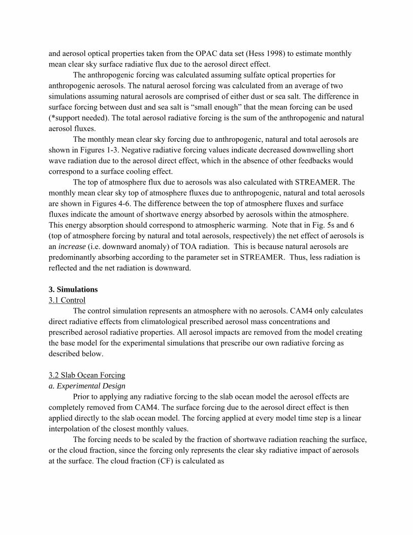
A control run with no aerosol interactions as well as nine forcing experiments were performed. Three sets of experiments apply the aerosol forcing to either the slab ocean model, the top of the atmosphere or the top of the atmosphere over oceans. Each set of experiments contains three simulations with anthropogenic, natural and total aerosol forcing applied in turn resulting in nine total experimental simulations. The nine model experiments are summarized in the table below. Table 1. Summary of nine model experiments. Forced Slab

Ocean Model (SOM)

Forced Top Of Atmosphere (TOA)

Forced Top Of Atmosphere -Over Oceans Only (TOA_Ocean)

Anthropogenic Aerosol Forcing

Anthro-SOM Anthro-TOA Anthro-TOA_Ocn

Natural Aerosol Forcing Natural-SOM Natural-TOA Natural-TOA_Ocn

Total Aerosol Forcing Total-SOM Total-TOA Total- TOA_Ocn

2. Forcing

The aerosol direct effect forcing (W/m2) applied in these experiments was determined through a simple radiative transfer model (STREAMER). STREAMER utilizes global climatological distributions of aerosol optical depth, obtained from Stefan Kinne (Kinne 2013),

and aerosol optical properties taken from the OPAC data set (Hess 1998) to estimate monthly mean clear sky surface radiative flux due to the aerosol direct effect.

The anthropogenic forcing was calculated assuming sulfate optical properties for anthropogenic aerosols. The natural aerosol forcing was calculated from an average of two simulations assuming natural aerosols are comprised of either dust or sea salt. The difference in surface forcing between dust and sea salt is “small enough” that the mean forcing can be used (*support needed). The total aerosol radiative forcing is the sum of the anthropogenic and natural aerosol fluxes.

The monthly mean clear sky forcing due to anthropogenic, natural and total aerosols are shown in Figures 1-3. Negative radiative forcing values indicate decreased downwelling short wave radiation due to the aerosol direct effect, which in the absence of other feedbacks would correspond to a surface cooling effect.

The top of atmosphere flux due to aerosols was also calculated with STREAMER. The monthly mean clear sky top of atmosphere fluxes due to anthropogenic, natural and total aerosols are shown in Figures 4-6. The difference between the top of atmosphere fluxes and surface fluxes indicate the amount of shortwave energy absorbed by aerosols within the atmosphere. This energy absorption should correspond to atmospheric warming. Note that in Fig. 5s and 6 (top of atmosphere forcing by natural and total aerosols, respectively) the net effect of aerosols is an increase (i.e. downward anomaly) of TOA radiation. This is because natural aerosols are predominantly absorbing according to the parameter set in STREAMER. Thus, less radiation is reflected and the net radiation is downward.

3. Simulations 3.1 Control The control simulation represents an atmosphere with no aerosols. CAM4 only calculates direct radiative effects from climatological prescribed aerosol mass concentrations and prescribed aerosol radiative properties. All aerosol impacts are removed from the model creating the base model for the experimental simulations that prescribe our own radiative forcing as described below. 3.2 Slab Ocean Forcing a. Experimental Design

Prior to applying any radiative forcing to the slab ocean model the aerosol effects are completely removed from CAM4. The surface forcing due to the aerosol direct effect is then applied directly to the slab ocean model. The forcing applied at every model time step is a linear interpolation of the closest monthly values.

The forcing needs to be scaled by the fraction of shortwave radiation reaching the surface, or the cloud fraction, since the forcing only represents the clear sky radiative impact of aerosols at the surface. The cloud fraction (CF) is calculated as

CF = FSDS/FSDSC (1) where FSDS is the shortwave downward flux at the surface, and FSDSC is the shortwave downward flux at the surface in clear-sky conditions. To avoid errors in regions with no solar radiation (i.e. polar night), CF is set to zero when FSDSC equals zero. The cloud fraction is calculated in the atmosphere component of the model before being passed through the model coupler to the slab ocean component.

The correctly scaled surface forcing is incorporated into the slab ocean through a change in the heat flux received. The change in ocean mixed layer temperature due to heat fluxes is determined by

, (2) where rho is the density of ocean water, cp is the specific heat, hmix is the depth of the mixed layer, Tmix is the temperature of the mixed layer (assumed to be the same as the surface temperature), Fnet is the net surface heat flux, and Qflx is the horizontal and vertical heat flux into and out of the mixed layer column. b. Results

Using a simple stochastic model (Deser 2003) the direct forced ocean mixed layer temperature response to the aerosol forcing is calculated. The stochastic model equation is

(ρCpH)dT’/dt = F’ – λT’ , (3)

where ρ is the density of sea water (1000 kg m-3), Cp is the heat capacity of water (4128 J kg-1 K-

1), H is the mixed layer depth, F’ is the atmospheric forcing of the mixed layer, T’ is the mixed layer temperature anomaly due to the atmospheric forcing, and λ is a linear damping coefficient (15 W m-2 K-1). This “direct” response is what would be expected in the absence of any response of the climate system, aside from a change in surface temperature. To calculate the seasonal cycle of T’, equation (3) is iterated forward using the seasonal cycle of surface forcing (F’). This provides a baseline estimate of what sort of response would be expected in the absence of any non-local atmospheric feedbacks. Figure 7 shows the mixed layer depth used in the slab ocean model. Prior to calculating the direct forced mixed layer temperature response, the anthropogenic, natural and total aerosol forcing are scaled by the climatological cloud fraction. The seasonal estimated direct forced temperature responses to each aerosol forcing are shown in Figures 8-10. The response is, by construction, very sensitive to the choice of linear damping coefficient.

When applying the forcing at the surface the atmosphere does not reach radiative equilibrium over climatological time scales. Figure 11 shows globally averaged time series of net, longwave and short wave fluxes at the top of the atmosphere for a model simulation with standard aerosol interactions (red), the control simulation with no aerosol interactions (blue) and

the simulation with our total aerosol forcing applied to the slab ocean model (black). The standard model simulation and the control simulation with no aerosols show a system in radiative equilibrium with a net flux of zero at the top of the atmosphere on climatological time scales. The simulation with aerosol forcing applied at the surface, however, shows approximately a 2 Wm-2 decrease in outgoing longwave radiation resulting in radiative energy imbalance at the top of the atmosphere.

3.3 Top of Atmosphere Forcing a. Experimental Design

As with the slab ocean experiments, the aerosol effects are completely removed from CAM4 prior to adding the aerosol forcing. The aerosol forcing is applied to the top of the atmosphere through an alteration in the solar insolation (SOLIN). This method corrects the net atmosphere energy imbalance that occurs when adding the forcing to only the surface, as well as allows forcing to be applied over land regions. The forcing is read into the atmosphere component as a new variable and applied at every time step as a linear interpolation of the closest monthly values.

In order to maintain the correct forcing at individual time steps within the diurnal cycle, which also results in the correct daily and monthly average forcing, the monthly average forcing is converted to the local-noon time values prior to being read into the atmosphere model. The local-noon clear sky forcing, shown in Figures 12-14, is calculated as

noon_forcing = avg_forcing / (SOLIN / tot_irrad.), (4)

where avg_forcing is the original clear sky surface radiative forcing as described in section 2, SOLIN is the solar insolation at the top of the atmosphere determined from the control simulation, and tot_irrad is the total irradiance (1361.27 W/m2). The local-noon forcing calculation removes effects of the solar zenith angle allowing the applied aerosol forcing to be correctly scaled by the diurnal cycle within the model.

The local noon forcing is applied to the model at the top of the atmosphere by altering the solar insolation calculation as below,

SOLIN = (tot_irrad + noon_forcing) * eccf * f(θ) , ( 5)

where SOLIN is the solar insolation, tot_irrad is the solar constant (1361.27 W/m2), noon_forcing is the applied aerosol forcing, eccf is the orbit eccentricity factor, and f(θ) is a function of the solar zenith angle, θ.

b. Results

The simple stochastic model (Eqn 3) is used to calculate the slab ocean model direct forced temperature response to aerosol forcing applied at the top of the atmosphere. Since the

aerosol forcing is applied at the top of the atmosphere, the net forcing received at the surface is needed to determine the direct slab ocean temperature response. The surface forcing over the ocean for each aerosol simulation is calculated as the clear sky downwelling shortwave surface flux anomaly from the control simulation scaled by the cloud fraction as follows,

F’ = CF * (FSDSC – FSDSC_control) , (6)

where F’ is the atmospheric forcing on the slab ocean model due to the applied aerosol forcing at the top of the atmosphere, CF is the cloud fraction as computed in Eqn 1, FSDS is the downwelling shortwave radiation flux at the surface for the experimental simulation, and FSDS_control is the downwelling shortwave radiation flux at the surface for the control simulation. The seasonally averaged direct forced mixed layer temperature responses due to aerosol forcing applied at the top of the atmosphere are shown in Figures 15-17.

The net forcing received at the ocean surface appears to be too weak when the aerosol forcing is applied at the top of the atmosphere. By applying the radiative forcing anomaly at the top of atmosphere, the total incoming shortwave radiation is reduced. As the atmosphere typically absorbs about 25% of incoming shortwave radiation, the reduction in top of atmosphere radiation also results in a reduction in atmospheric absorption. The anomaly at the surface, then, is reduced by about 25% due to reduced atmospheric absorption (less is absorbed by the atmosphere, so more reaches the surface). The change in clear sky atmospheric forcing on the slab ocean model when the aerosol forcing is applied at the top of the atmosphere (i.e. surface forcing difference between the top of atmosphere simulation and the surface forced simulation) is shown in Figures 18-20. Note the increase in downward radiation is larger than 25% of the applied anomaly. We suspect that this is due to a cooling of the atmosphere and hence a reduction in water vapor that is predominantly responsible for the atmospheric absorption. 3.4 Top of Atmosphere- Ocean Only Forcing a. Experimental Design

The model aerosol effects are completely removed from CAM4 prior to adding any aerosol forcing. These experiments apply the local noon forcing (Figures 12-14) to the top of atmosphere solar insolation over ocean regions only. The CAM4 land fraction variable, taken from the control simulation, is used to set all forcing values over land to zero. The forcing application method is the same as the previous set of experiments as explained in section 3.3a. b. Results

The simple stochastic model (Eqn 3) is used to calculate the slab ocean model direct forced temperature response to aerosol forcing applied at the top of the atmosphere over oceans only. The seasonal direct forced mixed layer temperature responses are shown in Figures 21-23. The direct temperature response to top of atmosphere aerosol forcing over oceans is similar to the previous set of experiments (Figures 15-17).

The forcing received at the ocean surface in these simulations is weaker than the forcing applied to the slab ocean model simulations. The surface temperature of slab ocean forced simulations appear to be warmer than the surface temperature of the top of atmosphere forced simulations. Figure 24 shows the difference in surface temperature between the slab ocean forced simulations and the top of atmosphere ocean only total aerosol forced simulations. 4. Discussion

The top of atmosphere and surface forced model experiments point out a problem with the experimental design of the model simulations. The coupled climate system response must involve both atmospheric and oceanic responses. By applying the aerosol forcing at either the upper or lower boundary, the atmosphere experiences an unrealistic absorption by non-aerosol constituents (which accounts for about 25% of shortwave radiation absorption). For example, consider the case of a completely reflective aerosol layer that is high in the atmosphere (this is analogous to our Top of Atmosphere Forcing simulations). Incoming radiation is reduced by the reflectivity a of the aerosol layer (a reduction of a*S0). This means that the atmosphere absorbs 0.25*a*S0 LESS radiation than it would in the absence of that aerosol layer, and is cooler as a result. In the case of a low-level aerosol layer that is purely reflective (this is analogous to our Surface Forcing experiments), the atmosphere absorbs MORE than it would in the absence of an aerosol layer due to absorption of the radiation that is reflected off of the aerosol layer.

Now, consider the climate system response to the two situations above. In the case of a high aerosol layer, the atmosphere cools due to reduced atmospheric absorption, and the surface cools due to reduced surface forcing. In a simple linear model, the atmosphere and ocean cool by comparable amounts, so the air-sea temperature difference does not change appreciably. In the case of a low aerosol layer, the ocean cools and the atmosphere warms. This reduces the air-sea temperature difference which consequently reduces the bulk aerodynamic fluxes (which tend to cool the ocean and warm the atmosphere). Hence, the surface does not cool as much. The situation is exacerbated substantially by the presence of absorbing aerosols. We note that in the case of short term fluctuations (such as those associated with short term dust variations) these issues are not as important. But, in an equilibrium climate simulation, the vertical distribution of aerosols is critical to the subsequent climate response.

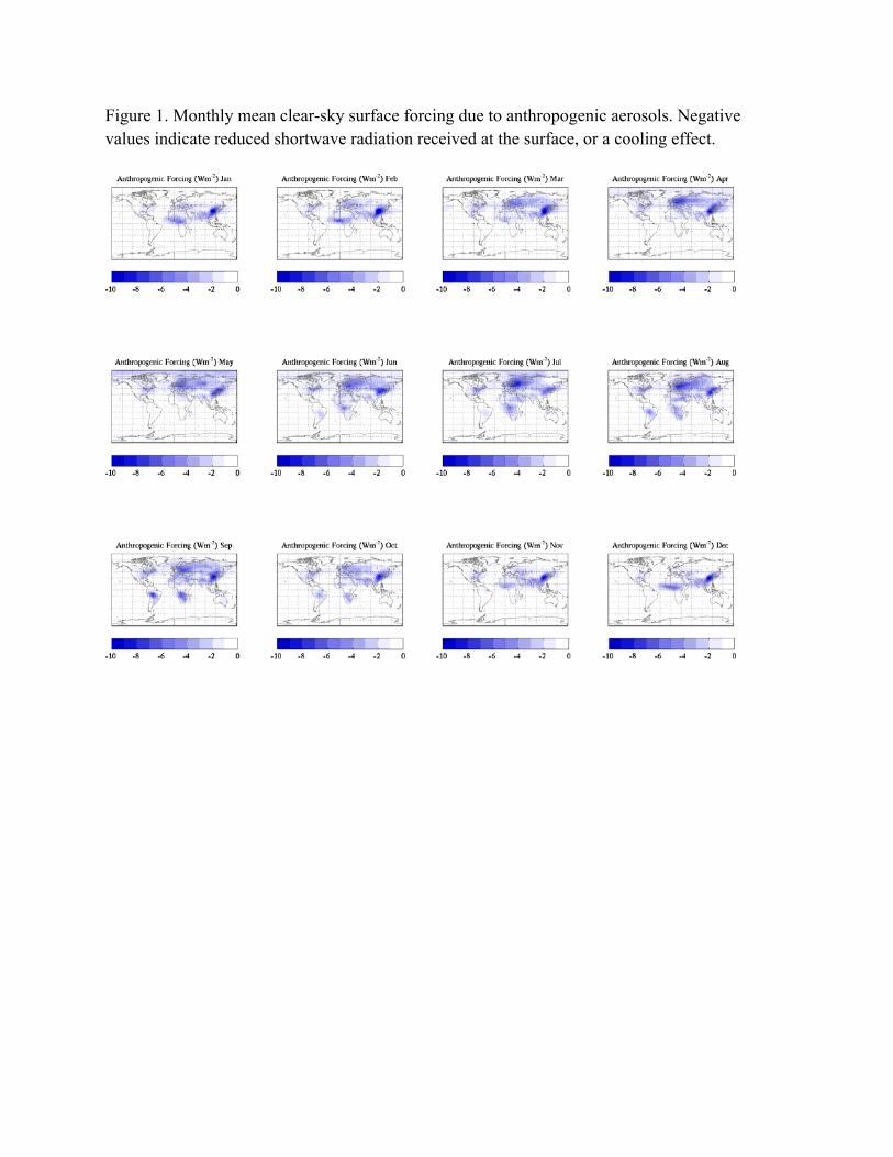
Figure 1. Monthly mean clear-sky surface forcing due to anthropogenic aerosols. Negative values indicate reduced shortwave radiation received at the surface, or a cooling effect.

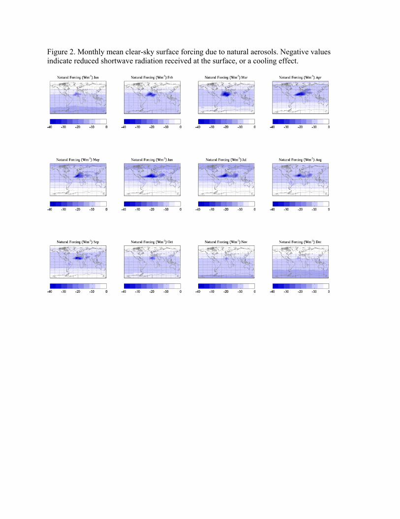
Figure 2. Monthly mean clear-sky surface forcing due to natural aerosols. Negative values indicate reduced shortwave radiation received at the surface, or a cooling effect.

Figure 3. Monthly mean clear-sky surface forcing due to total aerosols. Negative values indicate reduced shortwave radiation received at the surface, or a cooling effect.

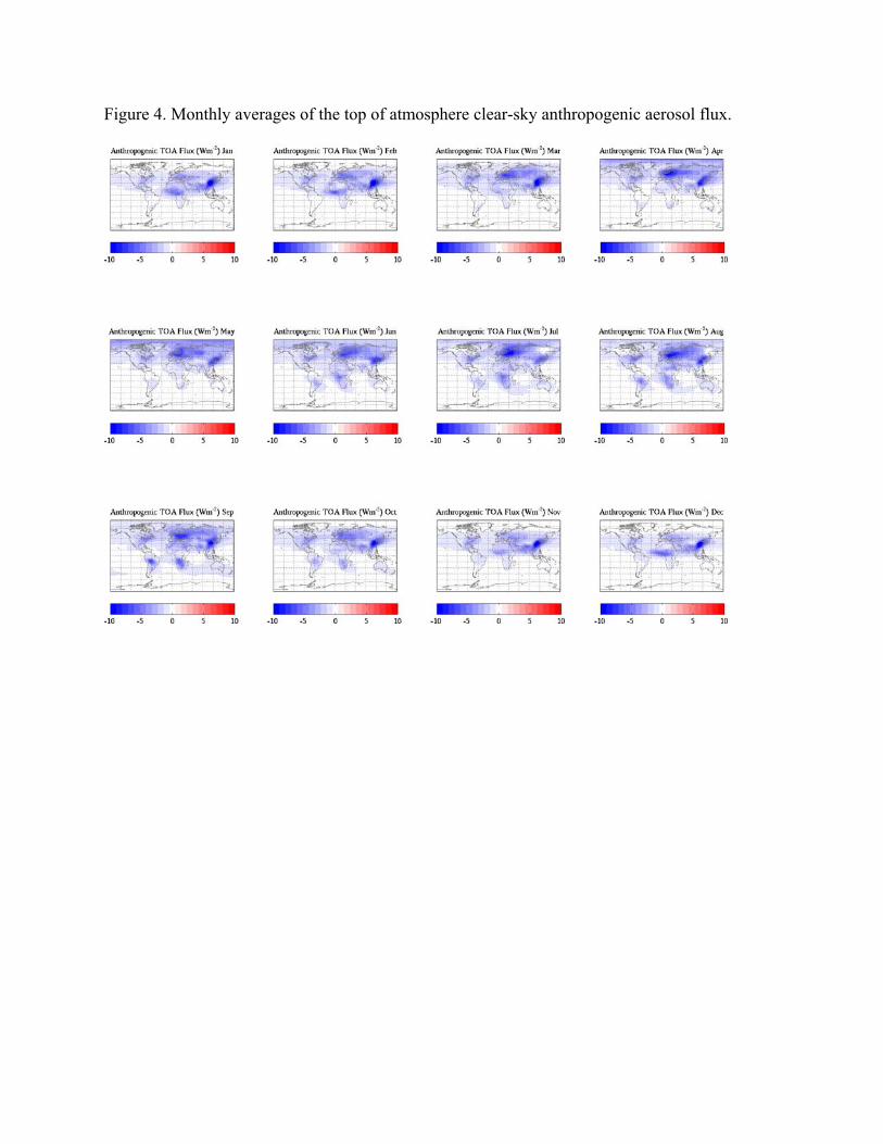
Figure 4. Monthly averages of the top of atmosphere clear-sky anthropogenic aerosol flux.

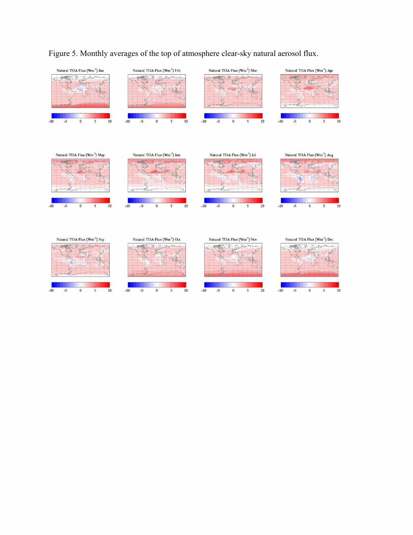
Figure 5. Monthly averages of the top of atmosphere clear-sky natural aerosol flux.

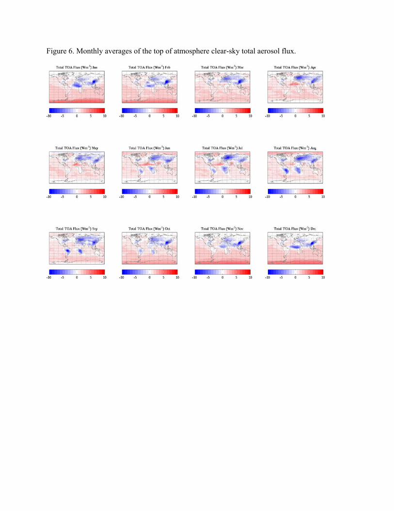
Figure 6. Monthly averages of the top of atmosphere clear-sky total aerosol flux.

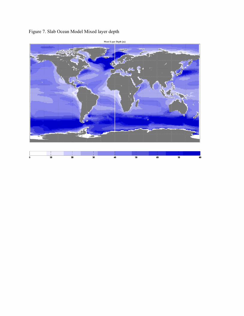
Figure 7. Slab Ocean Model Mixed layer depth

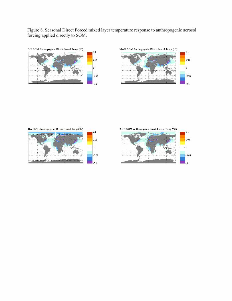
Figure 8. Seasonal Direct Forced mixed layer temperature response to anthropogenic aerosol forcing applied directly to SOM.

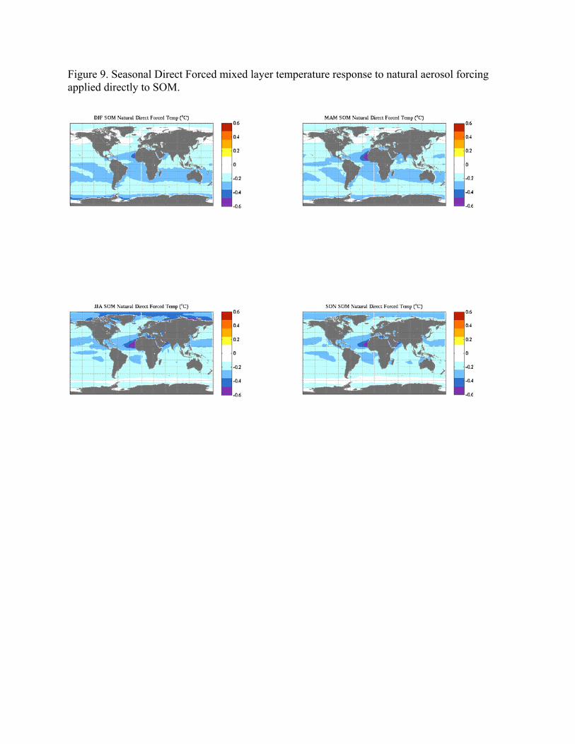
Figure 9. Seasonal Direct Forced mixed layer temperature response to natural aerosol forcing applied directly to SOM.

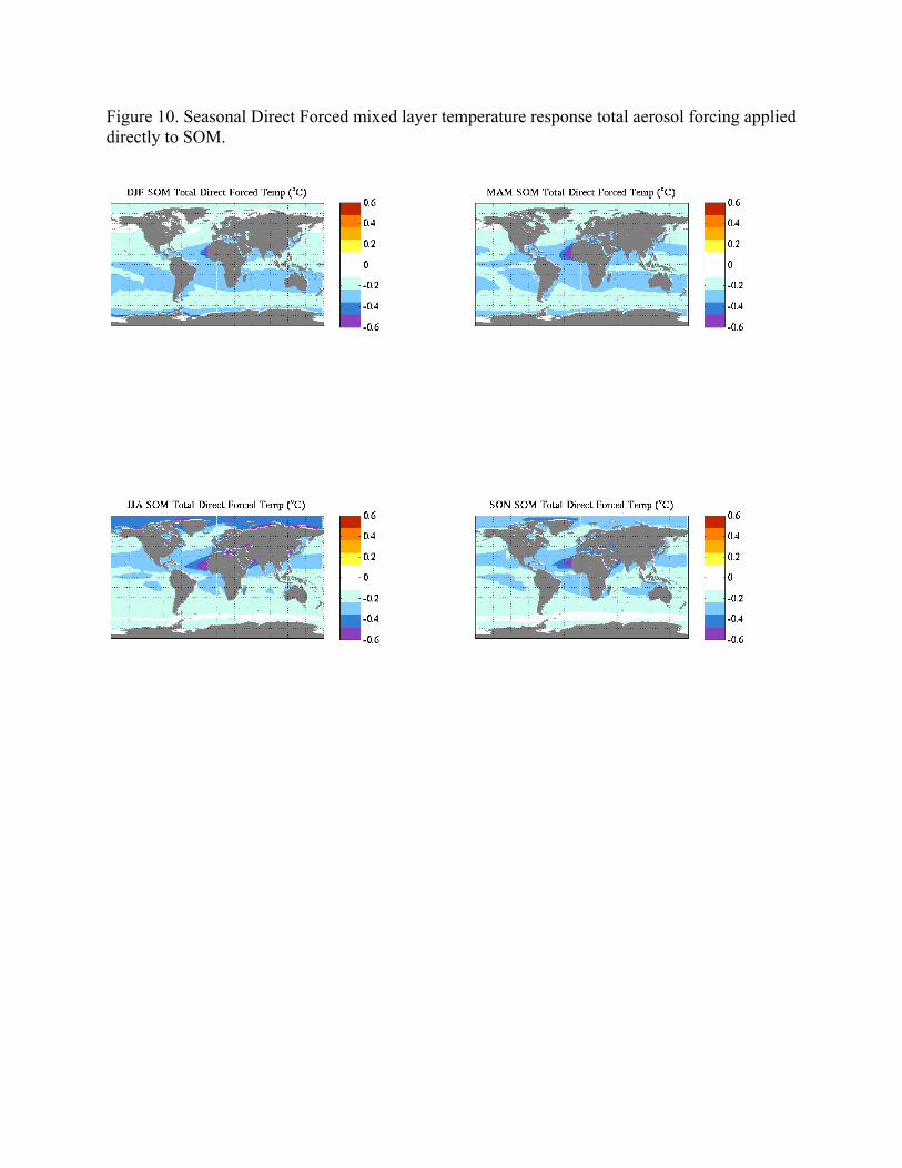
Figure 10. Seasonal Direct Forced mixed layer temperature response total aerosol forcing applied directly to SOM.

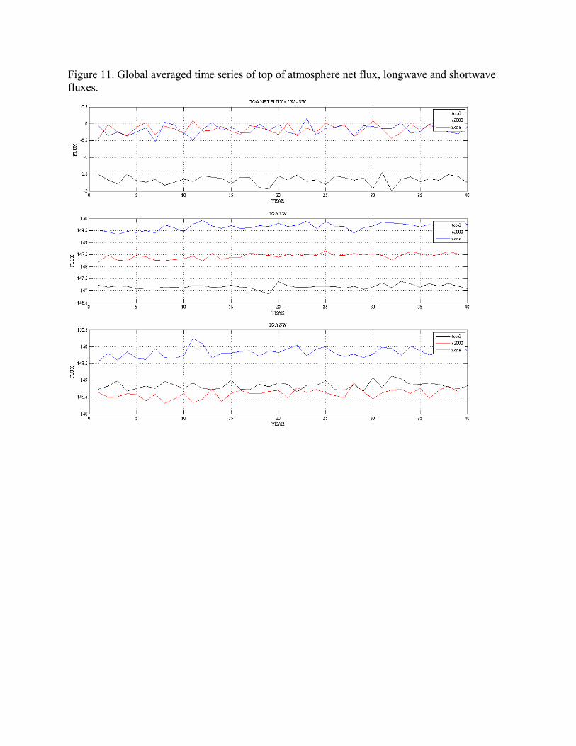
Figure 11. Global averaged time series of top of atmosphere net flux, longwave and shortwave fluxes.

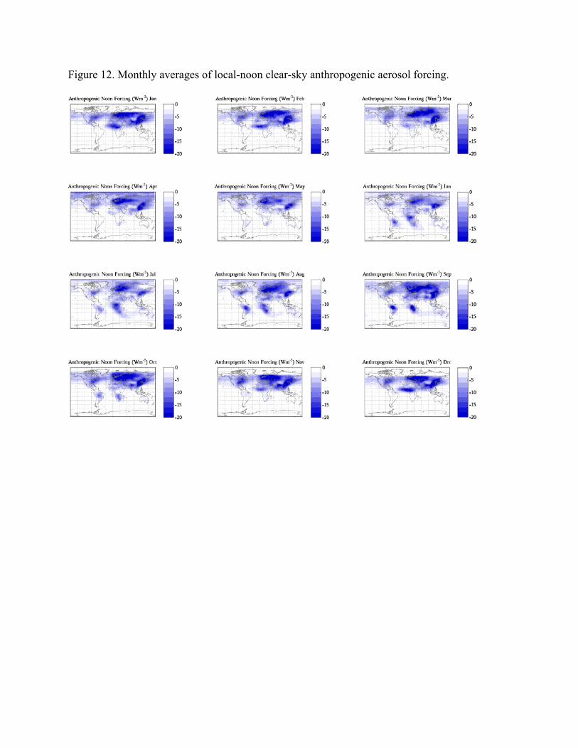
Figure 12. Monthly averages of local-noon clear-sky anthropogenic aerosol forcing.

Figure 13. Monthly averages of local-noon clear-sky natural aerosol forcing.

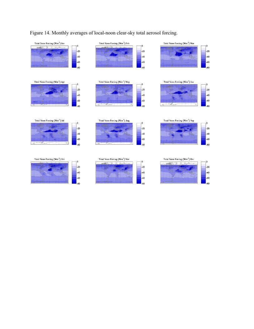
Figure 14. Monthly averages of local-noon clear-sky total aerosol forcing.

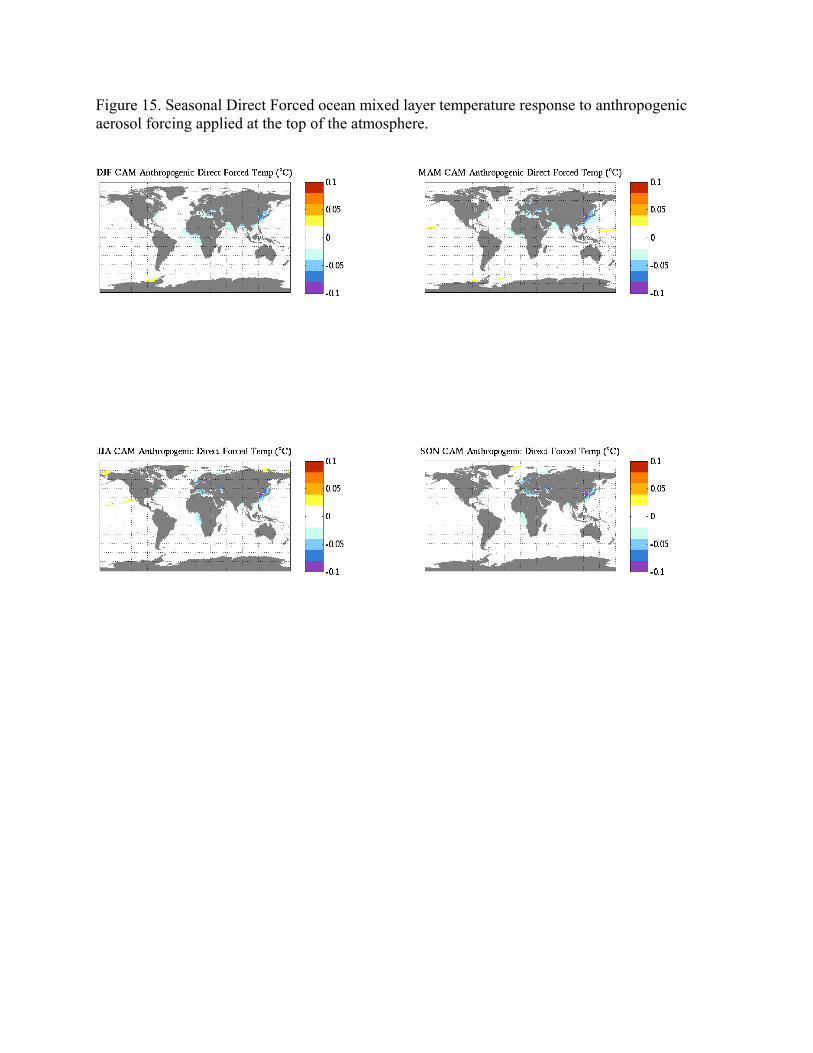
Figure 15. Seasonal Direct Forced ocean mixed layer temperature response to anthropogenic aerosol forcing applied at the top of the atmosphere.

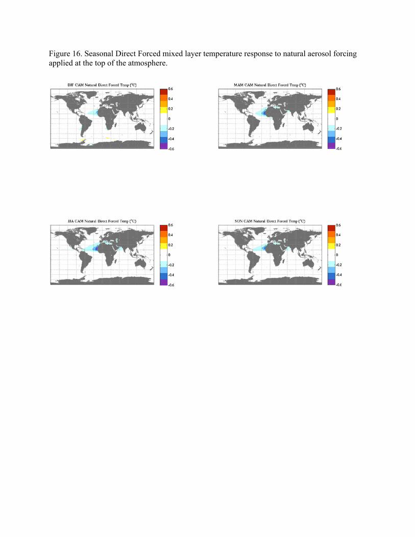
Figure 16. Seasonal Direct Forced mixed layer temperature response to natural aerosol forcing applied at the top of the atmosphere.

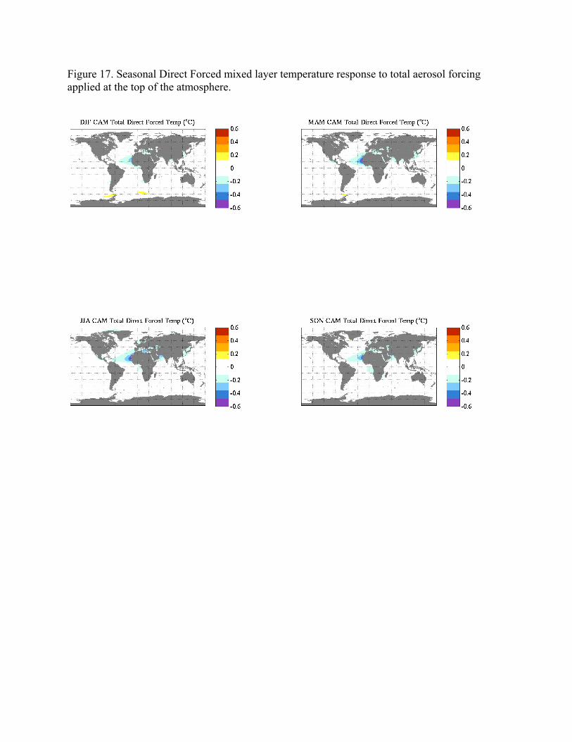
Figure 17. Seasonal Direct Forced mixed layer temperature response to total aerosol forcing applied at the top of the atmosphere.

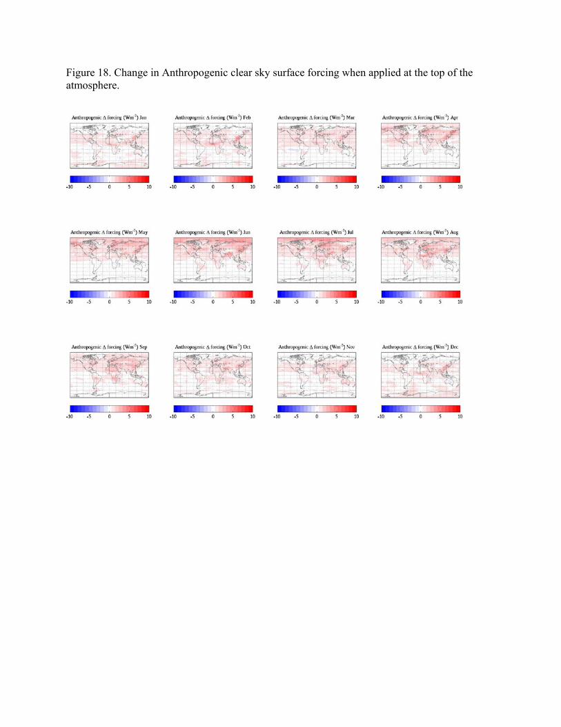
Figure 18. Change in Anthropogenic clear sky surface forcing when applied at the top of the atmosphere.

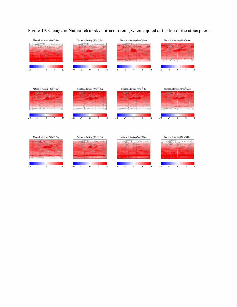
Figure 19. Change in Natural clear sky surface forcing when applied at the top of the atmosphere.

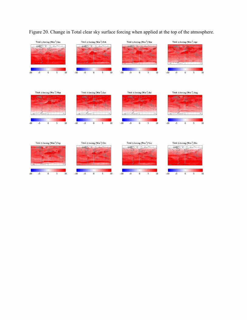
Figure 20. Change in Total clear sky surface forcing when applied at the top of the atmosphere.

Figure 21. Seasonal Direct Forced ocean mixed layer Temperature response to anthropogenic aerosol forcing applied at the top of the atmosphere over ocean regions only.

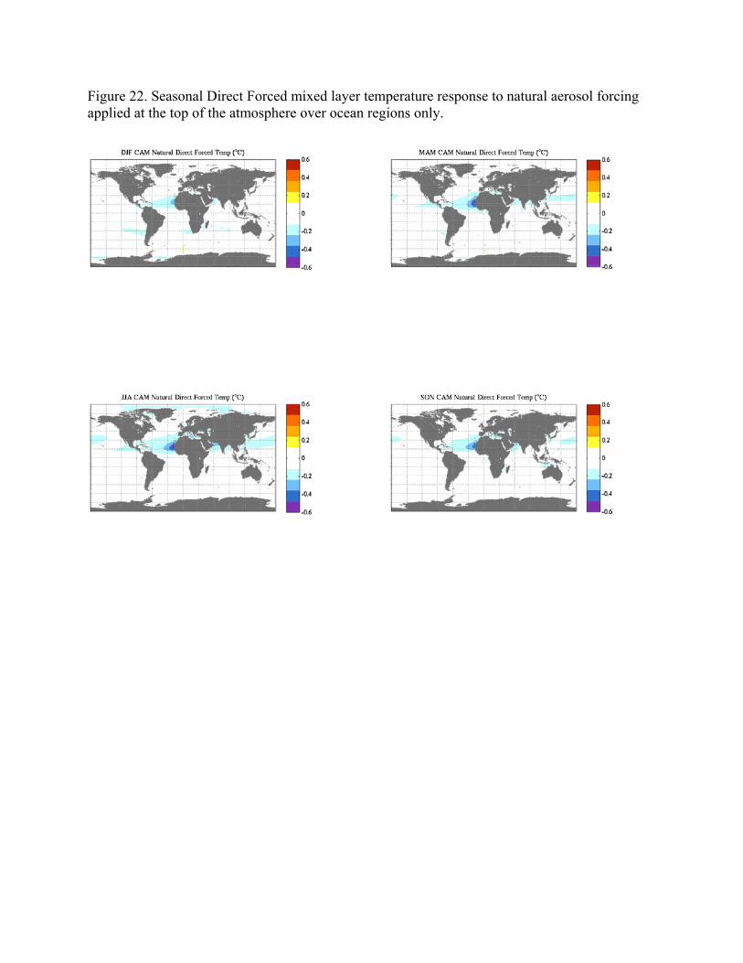
Figure 22. Seasonal Direct Forced mixed layer temperature response to natural aerosol forcing applied at the top of the atmosphere over ocean regions only.

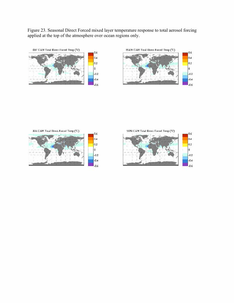
Figure 23. Seasonal Direct Forced mixed layer temperature response to total aerosol forcing applied at the top of the atmosphere over ocean regions only.

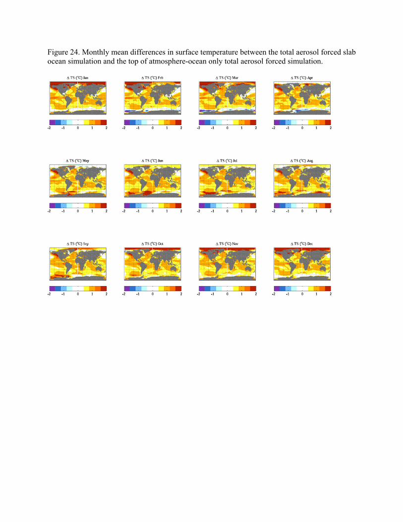
Figure 24. Monthly mean differences in surface temperature between the total aerosol forced slab ocean simulation and the top of atmosphere-ocean only total aerosol forced simulation.