data acquisition and processing report...convert to rinex trimble 2.1.7.0 convert gnss reference...

U.S. DEPARTMENT OF COMMERCE NATIONAL OCEANIC AND ATMOSPHERIC ADMINISTRATION NATIONAL OCEAN SERVICE

DATA ACQUISITION AND PROCESSING REPORT

Type of Survey Hydrographic

Project OPR-C308-KRL-13

Contract No DG133C-10-CQ-0059

Task Order No T-0002

Time Frame March 2014

LOCALITY

State New Jersey

General Locality New Jersey Coast and Vicinity

2014

CHIEF OF PARTY Carol Lockhart, David Evans and Associates, Inc.

LIBRARY & ARCHIVES

DATE

OPR-C308-KRL-13 New Jersey Coast and Vicinity March 2014 Data Acquisition and Processing Report Field Unit: David Evans and Associates, Inc.

i

TABLE OF CONTENTS

INTRODUCTION......................................................................................................................... 1

A. EQUIPMENT ........................................................................................................................... 1

A1. Data Acquisition Hardware and Software ............................................................................2 A1.a Aircraft .............................................................................................................................. 2

A1.b ChiropteraI Lidar System .................................................................................................. 3

A1.c GNSS Ground Control Equipment .................................................................................... 4

A1.d Aircraft Offset Survey Equipment ..................................................................................... 5

A2. Processing Software .............................................................................................................6

B. QUALITY CONTROL ............................................................................................................ 7

B1. Survey Methods & Procedures .............................................................................................7 B1.a Mobilization ...................................................................................................................... 7

B1.b Lidar Calibration .............................................................................................................. 8

B1.c Reconnaissance ............................................................................................................... 10

B1.d Survey .............................................................................................................................. 12

B2. Data Processing Methods & Procedures.............................................................................15 B2a. Data Management ........................................................................................................... 15

B2.b Field Processing .............................................................................................................. 15

B2.c Workflow Overview ......................................................................................................... 16

B2.d Trajectory Processing ..................................................................................................... 18

B2.e Lidar Processing ............................................................................................................. 19

B2.f Lidar Editing ................................................................................................................... 21

B2.g Datum Conversion .......................................................................................................... 23

B2.h Product Creation ............................................................................................................. 24

B2.i Imagery Processing ......................................................................................................... 26

B3. Additional Quality Checks ...............................................................................................27

C. CORRECTIONS TO ECHO SOUNDINGS ....................................................................... 29

C1. System Offsets ....................................................................................................................29

C2. Lidar Calibrations ...............................................................................................................29

C3. Motion Corrections .............................................................................................................29

C3. Environmental Parameters / Processing Settings ...............................................................29

C4. Vertical Datum Conversions...............................................................................................30

D. APPROVAL SHEET ............................................................................................................. 30

E. TABLE OF ACRONYMS ..................................................................................................... 32


ii

List of Figures Figure 1. Aircraft N7266Z used for survey .................................................................................... 3 Figure 2. The ChiropteraI System ................................................................................................... 4 Figure 3. Trimble R7 and Zephyr Geodetic Antenna on Point OCS_NJ_01 .................................. 5 Figure 4. Topcon GTS-212 Total Station ....................................................................................... 5 Figure 5. System Offset Survey at ACY ......................................................................................... 7 Figure 6. Example Calibration Flight Pattern ................................................................................. 8 Figure 7. Calibration Review Example ......................................................................................... 10 Figure 8. Nine Potential Areas & Reconnaissance Flight Lines ................................................... 11 Figure 9. Planned Flight Lines for Area 1 providing 200% Coverage ......................................... 13 Figure 10. Sample Operator Display ............................................................................................ 14 Figure 11. Overview of Data Processing Workflow ..................................................................... 17 Figure 12. Sample Waveform from Area 1 .................................................................................. 20 Figure 13. Sample LSS review screen from Area 1 ...................................................................... 21 Figure 14. VDatum Clipping in Area 6, Line 012_FL15 ............................................................. 23 Figure 15. Area 1 Example of High Uncertainty along Harbor Walls ......................................... 26 Figure 16. Co-registration of orthophoto mosaics and lidar intensity images .............................. 27

List of Tables Table 1. H12606 Hardware ............................................................................................................. 2 Table 2. Processing Software .......................................................................................................... 6 Table 3. GNSS Lever Arm Offset ................................................................................................... 8 Table 4. Calibration Corrections ..................................................................................................... 9 Table 5. Acquisition Parameters ................................................................................................... 12 Table 6. Base Stations Used for Trajectory Processing ................................................................ 18 Table 7. Trajectory Processing QC Results .................................................................................. 19 Table 8. H12606 LAS Classes ...................................................................................................... 23 Table 9. CUBE Parameters Used .................................................................................................. 24 Table 10. TPU Values Used for Every Point ................................................................................ 25 Table 11. Initial Comparisons to Known RTK Ground Truth ...................................................... 28 Table 12. Final Comparison to Known RTK Ground Truth (Area 1 Only) ................................. 28 Table 13. CrossLine Point to Surface Results .............................................................................. 28 Table 14. Cumulative VDatum Uncertainty ................................................................................. 30


1

Data Acquisition and Processing Report

Project OPR-C308-KRL-13 New Jersey Coast and Vicinity March 2014

N7266Z David Evans and Associates, Inc.

Chief of Party: Carol Lockhart

INTRODUCTION

This report applies to surveys for H12606 located along the New Jersey coast and vicinity. These contract surveys were performed under OPR-C308-KRL-13 as specified in the Statement of Work (June, 2013) and Hydrographic Survey Project Instructions (June 18, 2014). All survey methods meet or exceed requirements as defined in the National Ocean Service (NOS) Hydrographic Surveys Specifications and Deliverables (HSSD) (April 2013). The survey consisted of 200 percent topographic and bathymetric lidar coverage within three of the nine potential survey polygons depicted in the Project Reference File OPR-C308-KRL-13_PRF.000 which was included with the Hydrographic Survey Project Instructions. No Automated Wreck and Obstruction Information System (AWOIS) items were required for this project.

A. EQUIPMENT

For this project David Evans and Associates, Inc. (DEA), along with Geomatics Data Solutions, LLC. (GDS), installed an Airborne Hydrography, AB (AHAB) ChiropteraI Topographic and Bathymetric Lidar system into a Quantum Spatial (QSI) Cessna 206 (Tail N7266Z) in accordance with modern remote sensing techniques. Operational systems used to acquire survey data are described in detail in this section and are listed in Table 1.


2

Table 1. H12606 Hardware

Instrument Manufacturer Model Serial No. Function ChiropteraI Topographic (300kHz) and Bathymetric (35kHz) Lidar System

ChiropteraI, which includes:

AHAB Version 1 1 Topographic (300kHz) and Bathymetric (35kHz) lidar sensor

IGI AEROcontrol with IMU-IIe & GNSS Antenna

Flight Control Software Positioning and Inertial Reference System for position, heading, roll and pitch.

iDS µEye UI-2280SE Digital RGB 5MP Camera (2560 x 1920) acquiring at 1 frame per second (fps)

Ground Control / Ground Truth

GNSS Receiver Trimble R7 7600 GNSS Base Receiver

GNSS Antenna Trimble Zephyr Geodetic Model 2 RoHS

1004 GNSS Base Antenna (TRM57971.00)

GNSS Receiver Trimble R7 9151 GNSS Base Receiver

GNSS Antenna Trimble Zephyr Geodetic Model 2 RoHS

8162 GNSS Base Antenna (TRM57971.00)

GNSS Rover Trimble R6 Model 3 7238 GNSS Rover with integrated antenna (TRMR6-3)

GNSS Rover Trimble R8 Model 2 0649 GNSS Rover with integrated antenna (TRMR8_GNSS)

Offset Survey

Total Station Topcon GTS-212 LH1749 Total Station used to measure sensor offsets

Prism / Reflectors Sokkia Reflective Stickers

A1. Data Acquisition Hardware and Software

A1.a Aircraft

A single engine Cessna 206 (Tail N7266Z) owned and operated by QSI (Figure 1) was the survey aircraft for the project. The aircraft has a transit speed of approximately 160 knots and an endurance of up to five hours. The aircraft has a photogrammetric port in the belly, and is commonly used for aerial survey. The ChiropteraI was installed in the main cabin, with pilot guidance positioned in the cab. The operator sat up front in the cab to control the ChiropteraI while airborne. A dual frequency 2 Hz high gain aerial Global Navigation Satellite System (GNSS) antenna (an integrated part of the AeroControl positioning system) was installed on the roof of the aircraft for positioning.


3

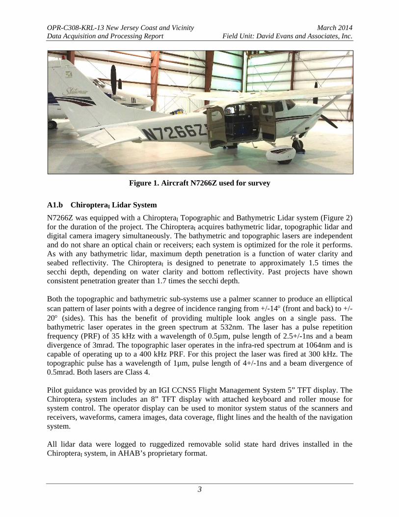
Figure 1. Aircraft N7266Z used for survey

A1.b ChiropteraI Lidar System

N7266Z was equipped with a ChiropteraI Topographic and Bathymetric Lidar system (Figure 2) for the duration of the project. The ChiropteraI acquires bathymetric lidar, topographic lidar and digital camera imagery simultaneously. The bathymetric and topographic lasers are independent and do not share an optical chain or receivers; each system is optimized for the role it performs. As with any bathymetric lidar, maximum depth penetration is a function of water clarity and seabed reflectivity. The ChiropteraI is designed to penetrate to approximately 1.5 times the secchi depth, depending on water clarity and bottom reflectivity. Past projects have shown consistent penetration greater than 1.7 times the secchi depth. Both the topographic and bathymetric sub-systems use a palmer scanner to produce an elliptical scan pattern of laser points with a degree of incidence ranging from +/-14 (front and back) to +/-20 (sides). This has the benefit of providing multiple look angles on a single pass. The bathymetric laser operates in the green spectrum at 532nm. The laser has a pulse repetition frequency (PRF) of 35 kHz with a wavelength of 0.5µm, pulse length of 2.5+/-1ns and a beam divergence of 3mrad. The topographic laser operates in the infra-red spectrum at 1064nm and is capable of operating up to a 400 kHz PRF. For this project the laser was fired at 300 kHz. The topographic pulse has a wavelength of 1µm, pulse length of 4+/-1ns and a beam divergence of 0.5mrad. Both lasers are Class 4. Pilot guidance was provided by an IGI CCNS5 Flight Management System 5” TFT display. The ChiropteraI system includes an 8” TFT display with attached keyboard and roller mouse for system control. The operator display can be used to monitor system status of the scanners and receivers, waveforms, camera images, data coverage, flight lines and the health of the navigation system. All lidar data were logged to ruggedized removable solid state hard drives installed in the ChiropteraI system, in AHAB’s proprietary format.


4

The system includes an IGI AEROControl Inertial Measurement Unit (IMU) and GNSS antenna for sensor position and attitude measurements. This included an IMU-IIe IMU with a sampling rate of 256 Hz and an accuracy in roll, pitch and heading of 0.004º, 0.004º and 0.01º respectively. All raw position and IMU data were recorded to a removable flash storage card inside the ChiropteraI System in IGI’s .c5l format.

Figure 2. The ChiropteraI System

A1.c GNSS Ground Control Equipment

In order to compute an accurate aircraft trajectory for final lidar processing, the aircraft GNSS and IMU data is post processed using ground based GNSS reference station data. For this project, some ground reference stations were established. In addition existing CORS stations were also used for ground reference stations on some flights. For points which were established for ground reference stations, Trimble R7 GNSS receivers were used to collect GNSS data. Each R7 was coupled with a Zephyr Geodetic Model 2 RoHS GNSS Antenna (Figure 3). Ground control points were also acquired with a Trimble R6 GNSS rover with integrated antenna.


5

Figure 3. Trimble R7 and Zephyr Geodetic Antenna on Point OCS_NJ_01

A1.d Aircraft Offset Survey Equipment

The aircraft offset survey was conducted using a Topcon GTS-212 Total Station, last calibrated on November 11, 2013. Sokkia reflective survey stickers were used in place of a prism to provide an accurate location of points collected.

Figure 4. Topcon GTS-212 Total Station


6

A2. Processing Software

A list of processing software used during the project is provided in Table 2. How each software was used and configured is described in detail in Section B of this report. All data were processed using Windows 7 and Windows 8 64-bit computers. Data was stored on removable USB 3.0 hard disks while in the field and moved to QNAP NAS for office data processing. At least two copies of the data existed at all times for backup and redundancy.

Table 2. Processing Software

Description Manufacturer Version Description

IGIPlan IGI 1.5 Flight Planning AeroOffice IGI 5.3e Trajectory Processing Waypoint GrafNav Novatel 8.40 GNSS Processing

Convert to RINEX Trimble 2.1.7.0 Convert GNSS Reference data to RINEX

Lidar Survey Studio (LSS)

AHAB 2.00.07 Airborne Data Processing

Terrascan Terrasolid 014.013 Lidar Editing MicroStation v8i Bentley 08.11.09.459 Lidar Editing with Terrascan

VDatum NGS 3.3 Convert LAS data from NAD83 to Tide Datum

Fledermaus QPS 7.3.6 QC, Final Processing, CUBE and BAG

ArcGIS ESRI 10.2.2 Project Planning, Interim QC, Product Review

Bathy DataBASE (64-bit)

CARIS 4.1 S-57, BASE Surface

OrthoMaster Inpho 5.5 Orthorectify Images

OrthoVista Inpho 5.5 Mosaic images

QT Modeler Applied Imagery 8.0.3 Intensity Images, Interim QC

FME Desktop Safe Software 2014, SP3 Convert BAG to .csar

Other

Microsoft Office Suite Microsoft 2013, 2007 Beyond Compare Beyond Compare 3.3.1


7

B. QUALITY CONTROL

B1. Survey Methods & Procedures

B1.a Mobilization

The ChiropteraI System was installed into a Cessna 206 (Tail N7266Z) at Capital City Airport in Frankfort, Kentucky on March 26, 2014. The system can be installed in either a forward or reverse direction, depending on the physical space requirements within the aircraft. The system was installed in the forward configuration for this project. Once the system was installed in the aircraft, an offset survey was performed to derive the offsets from the GNSS antenna to the IMU center in the IMU coordinate reference frame. During this first offset survey, issues keeping the total station level were encountered. This offset dataset was not used for the project. A second offset survey was performed at Atlantic City International Airport (ACY) on March 30, 2014 using a different total station, tribrach and tripod (Figure 5). Measurements were taken of the system case corners, random points on the sides of the system case, and points around the base and top of the GNSS antenna. Since a data logger was not used, measurements were logged to an Excel spreadsheet. Measurements were then processed with an AHAB proprietary script in MatLab to compute the final offsets. In general measurements to the side of the system case are used to help better define the plane of the system case side and therefore improve the corner coordinate measurements. The offset from the corners of the system case to the IMU center is known and fixed. Final offsets used for the project are provided in Table 3. These were used for all data processing including the calibration and reconnaissance flights acquired prior to March 30, 2014.

Figure 5. System Offset Survey at ACY


8

Table 3. GNSS Lever Arm Offset

Offset (m) StDev

X -0.112 0.0009 Y 0.108 0.0008 Z -0.813 0.0004

B1.b Lidar Calibration

Immediately following system installation, a calibration flight was conducted over the airport on March 26, 2014. A second calibration flight was conducted at the end of the survey over ACY on April 3, 2014. A calibration flight consists of about 6 to 12 flight lines with about 50% overlap between adjacent lines as shown in Figure 6. Ideally the calibration lines will cover certain types of features, including a large flat area or an area with a gentle even slope, and buildings with slant roofs. The buildings are acquired in perpendicular directions. The calibration site can also include known ground control points. These can be used during the calibration routine, or for validation. For this project known points were used for validation only.

Figure 6. Example Calibration Flight Pattern

The calibration data is used to eliminate systematic errors by calculating corrections for boresight errors, scanner angle errors, remaining IMU angle errors and any necessary slant range errors. System bias variables determined during calibration are provided in Table 4.


9

Table 4. Calibration Corrections

Correction Type

Description Parameters

Boresight Misalignment between the laser and optical axis Theta, Phi

Scanner Angle Errors in the mounting of the mirrors and scanner encoder values

Encoder, Alpha

IMU Angle Misalignment between the IMU and optical axis Roll, Pitch, Heading

Slant Range Distance measurement error due to delays, fiber lengths, etc.

Range

Data from the calibration flights are processed initially using calibration values from a prior installation in Lidar Survey Studio (LSS). Over the course of multiple projects, it has been found that calibration values change very little within the ChiropteraI system, indicating the system to be robust, even during shipping. Processed data is provided to the automatic calibration routine for analysis. The automatic calibration routine sets up a number of constraints and then uses an optimization algorithm to minimize the error estimation. For both calibration sets for H12606 constraints were in the form of patches. Patches are areas of relatively flat ground that are used for calibration. An automated routine was used to select suitable patches of flat ground from a number of lines. Patch locations selected can be reviewed to ensure even distribution over the calibration site before continuing with the calibration analysis. Once patches have been selected, data falling within these patches are then compared in two ways: first within a single line, the front and back half of the elliptical scans are analyzed, and secondly with data from multiple lines. This is done automatically by the optimization algorithm which generates recommended calibration values. Lidar data from the calibration flight are then reprocessed in LSS using the new values and reviewed for accuracy. The accuracy review involves a visual comparison to ensure there are no position misalignments in the horizontal or vertical. Review includes, but is not limited to, a comparison of:

the front and back scan in cross section multiple lines in cross section over flat and undulating terrain multiple lines over significant features such as the building roof tops intensity for multiple lines over easily identified features such as parking lot lines

Review examples are provided in Figure 7. Calibration values calculated by the automated routine were deemed acceptable by the hydrographer and used for processing. Calibration values from the initial flight on March 26, 2014 were applied to all lidar data acquired from March 26, 2014 up to April 1, 2014. Calibration values from the flight over ACY on April 3, 2014 were applied to all lidar data acquired from April 2, 2014 up to April 3, 2014.


10

Figure 7. Calibration Review Example

Two calibration files were used for the project due to a firmware upgrade mid-project. After the reconnaissance flight on March 27, 2014 it was noticed that a larger volume of data than normal was being generated by the sensor. Data quality was not affected by this; however a small adjustment was made to the acquisition settings to reduce the number of files being generated by the system. Unfortunately the setting adjustments caused the bathymetric waveforms to be clipped for the second acquisition flight over Area 1 on April 1, 2014. This data was not usable and was not included in any further processing or products generated for H12606. A firmware upgrade was made from CATbtopV25 to CATbtopV31 before flights commenced on April 2, 2014. This required an update to the calibration, and the calibration data were collected on April 3, 2014. B1.c Reconnaissance

Nine potential survey areas were identified by NOAA and provided in OPR-C308-KRL-13_PRF.000. The areas were numbered in order of priority with Area 1 being the highest priority and Area 9 being the lowest priority (Figure 8). As defined in the project instructions, the project was limited to 20 hours of flying. Initially a reconnaissance flight acquired data over all areas to identify those with the best water clarity giving the most chance for success. Reconnaissance flight lines were planned such that the line for each area would cover a range of depths, from land across deeper channels. This would give an indication of depth penetration for the area. Reconnaissance data were acquired on March 27, 2014 and processed that evening for review. Reconnaissance data were acquired using the same survey parameters used during project data acquisition (Table 5). Analysis of this reconnaissance data, along with the area priority, were used to determine which areas would be the focus for the remaining flight hours. Areas 1 and 2 were initially selected, having the best water clarity and being the highest priority areas. Upon completion of Areas 1 and 2, there were enough flight hours remained to complete a third area. Area 6 was selected,


11

due to its promising water clarity during the reconnaissance flight and its proximity to the base airport. All areas selected were approved by the NOAA COTR in advance of data collection.

Figure 8. Nine Potential Areas & Reconnaissance Flight Lines


12

B1.d Survey

All survey data collection was conducted from 400m altitude at around 97 knots. The ChiropteraI simultaneously acquired bathymetric lidar at 35 kHz, topographic lidar at 300 kHz and digital camera imagery at one frame per second. These survey parameters produced a nominal pulse spacing of 0.75 meters for the bathymetric laser, 0.25 meters for the topographic laser and a ground sample distance of 25 centimeters for the rectified imagery mosaic for 100% coverage. The project required 200% bathymetric lidar coverage at a 1m x 1m laser spot spacing. To achieve this, hydrographic lidar flights were planned using the parameters provided in Table 5. All areas were flown to provide 200% coverage as required in the project instructions. Parameters used during survey operations exceeded the project requirements.

Table 5. Acquisition Parameters

Sensor ChiropteraI

Survey Altitude (AGL) 400m

Pulse Repetition Frequency (PRF) 35kHz Bathy, 300kHz Topo

Swath Width 290m

Coverage 200%

Nominal Spot Spacing 0.75 x 0.75m Bathy, 0.25m x 0.25m Topo

Maximum Number of Returns per Pulse 4

Data were collected at high tide and low tide for each area. One flight plan was created for each area at high tide, using a 225-meter line spacing to provide 122% coverage. A second flight plan was created for the low tide flights, with lines offset by 112.5 meters from the high tide lines. An example for Area 1 is provided in Figure 9. This provides the maximum number of look angles available for the project while providing the required 200% coverage. Crosslines were planned perpendicular to main scheme survey lines such that the lineal miles of crosslines would exceed the required 4% of main scheme survey lines as stated in the NOS HSSD (April 2013). The same crosslines were acquired at both high and low tide.


13

Figure 9. Planned Flight Lines for Area 1 providing 200% Coverage


14

Each flight followed the following general acquisition methodology:

Communicate with ground crew to ensure GNSS reference stations running Check hard disks are installed in system Review installation for any issues such as cable security Start GNSS/IMU under battery power Start engines Static initialization of GNSS (optional depending on base station location) Take off In air initialization over the base station (optional depending on base station location) Survey In air close out of GNSS session over the base station (optional depending on base station

location) Shut Down lidar System Land Static close out of GNSS session (optional depending on base station location) Shutdown engines Shutdown GNSS/IMU Remove data drives and return to office. Communicate with ground crew that flight is

complete. During data acquisition the operators display was used to select flight lines, which were then displayed on the pilot’s flight management system. In addition, the operator monitored system status of the scanners and receivers, waveforms, camera images, data coverage, flight lines and the health of the navigation system (Figure 10).

Figure 10. Sample Operator Display


15

The operator made notes of the general environmental conditions and any issue that occurred during flight, such as line restarts. A flight acquisition log was generated upon return to the office that included all relevant survey information for the flight. Flight logs are provided in the accompanying H12606 DR, Separate I. Aircraft bank angles were restricted to 20º to avoid any potential GNSS dropouts. No flights were planned if the PDOP was expected to go above 3.0. Positioning of the aircraft in real-time was accomplished by the integrated IGI AEROControl IMU and GNSS antenna. No real time corrections were used and no IMU data was used to steer the scan to aid in line-keeping. All lidar system data were logged to AHAB’s proprietary format on two ruggedized removable solid state hard drives. All raw position and IMU data were recorded to a removable flash storage card inside the ChiropteraI System in IGI’s .c5l format.

B2. Data Processing Methods & Procedures

B2a. Data Management

Upon return to the field office, data from the aircraft were copied onto two sets of external USB 3.0 hard disks to provide data redundancy. GNSS reference station data were sent via FTP and duplicate copies were also made of this data. On completion of the field work, processing was moved to the Geomatics Data Solutions office in San Diego. All data were stored on NAS and replicated nightly for backup. In addition, a copy of all the raw data was sent to David Evans and Associates office in Vancouver, WA where it was housed on an additional NAS and also subject to nightly backups. Upon completion of data processing a full copy of the data were placed on the DEA NAS, where final S-57 and BASE surface production was conducted. All data were organized according to Geomatics Data Solutions established directory structure for lidar processing. Standardized naming conventions were used throughout to maintain data integrity. B2.b Field Processing

Initial data processing followed the trajectory and LSS processing steps described in detail in the following sections. However due to the short duration of the project, initial field processing made use of preliminary calibration and trajectory files. Data were reviewed in LSS for data coverage and also to ensure there were no potential system issues. Data were not taken further in the processing work flow during field operations. The only system issue occurred during the second flight on April 1, 2014, when bathymetric waveforms were clipped before the seabed was reached. No data from this flight was used. Feedback was provided to the operator and a system modification was made before the next flight, allowing successful data collection on April 2, 2014.


16

B2.c Workflow Overview

An overview of the processing workflow is provided in Figure 11. In general data were processed in LSS using final processed trajectory information. LAS files from LSS were then imported to a Terrascan project where spatial algorithms were used to remove noise, mostly on the water surface. Manual editing was also conducted at this stage, with the entire data set being reviewed by a hydrographer. LAS files were exported by flight line from Terrascan and converted to mean lower low water (MLLW) using VDatum. In addition features pertinent to S-57 development were exported as ASCII XYZ files for import to CARIS Bathy DataBASE. LAS files on MLLW were imported to a Fledermaus project and a Fledermaus PFM file created with a Combined Uncertainty and Bathymetry Estimator (CUBE) surface. This CUBE surface was reviewed and soundings designated as necessary. Designated soundings were applied to the surface and the surface exported as a BAG, which contained a depth and uncertainty layer. The BAG was imported to CARIS Bathy DataBASE and a BASE surface created. The BASE surface was finalized, clipping to the average MHW height for the area.


17

Figure 11. Overview of Data Processing Workflow


18

B2.d Trajectory Processing

Airborne GNSS and IMU data were processed along with ground GNSS reference station data in AeroOffice. Airborne and ground GNSS data were processed together using GrafNav. Processing made use of both GPS and GLONASS satellites for positioning. This final GNSS solution was combined with the IMU data, taking in to account the GNSS antenna lever arm, to compute a final trajectory for the center of the IMU. GNSS data were processed in NAD83 (2011) and final trajectory solutions were exported from AeroOffice in a custom ASCII format for use in LSS processing. Final trajectory solutions were also in NAD83 (2011). Reference points established specifically for project H12606 and existing CORS stations were used for trajectory processing as provided in Table 6. During processing QC plots were reviewed both at the GNSS processing stage and also after final IMU processing. A summary of trajectory processing QC statistics are provided in Table 7. The Trajectory Processing Log is provided in the H12606 DR, Separate I. Point OCS_NJ_01 was established for use while flying Area 1, however GLONASS ephemeris data showed GLONASS satellites as turned off part way through April 1, 2014. This affected data acquired at the OCS_NJ_01 base station. Data were subsequently processed with CORS station data from NJGT and NJOC. No degradation in data accuracy occurred.

Table 6. Base Stations Used for Trajectory Processing

Date Flight Area(s)

Surveyed

Base Stations

Used Description

2014-03-26 A Calibration 84980850 Existing point used regularly by QSI at their Frankfort, KY base airport

2014-03-27 A Reconnaissance NJGT Existing CORS

2014-04-01 A Area 1 NJGT, NJOC Existing CORS, Bad GLONASS on OCS_NJ_01

2014-04-02 A Area 2 OCS_NJ_02 Point established for project

B Area 1 & 2 OCS_NJ_02, NJGT, NJOC

2014-04-03 A Area 6 DN8307 Existing marker, coordinates

established by QSI for separate NGS Sandy project B

Area 6, ACY Cal

DN8307


19

Table 7. Trajectory Processing QC Results

Date Flight

Trajectory Forward / Reverse Difference

X RMS (m)

Y RMS (m)

Z RMS (m)

2014-03-26 A 0.007 0.008 0.031 2014-03-27 A 0.007 0.007 0.033 2014-04-01 A 0.005 0.007 0.025

2014-04-02 A 0.009 0.009 0.029 B 0.006 0.006 0.025

2014-04-03 A 0.010 0.012 0.037 B 0.007 0.007 0.032

B2.e Lidar Processing

Airborne lidar data were processed using AHAB’s Lidar Survey Studio (LSS). During this stage raw airborne data is combined with system offsets, trajectory and calibration information to produce an accurately georeferenced lidar point cloud, with additional attributes associated to each point. During this processing routine LSS automatically discriminates between land and water points from the bathymetric laser. If a point is over water, then the point is automatically refracted to provide the correct final depth. No additional processing is necessary to refract data. Prior to processing the hydrographer can adjust waveform sensitivity settings dependent on the environment encountered and enter a value for the refraction index to be used for bathymetry. For this project, water salinity and temperature were monitored at the USGS water gage (01408167) and the average values during each flight were used, along with the laser wavelength of 532nm, to calculate an index of refraction number for processing of the bathymetric lidar data within each survey area. Values used are included in the LSS processing settings files delivered with the raw data for the project. In the field, default waveform sensitivity settings were used for processing. In order to determine the optimal waveform sensitivity settings for final processing, sample areas were selected and processed with multiple different settings, to iteratively converge on the best possible settings. This is done by reviewing the processed point cloud and waveforms within the sample areas. Settings affect which waveform peaks are classified as valid seabed, and which peaks are classified as noise. Optimal settings strike a balance between the amount of valid data that is classified as seabed bottom, and the amount of noise that is incorrectly classified due to peaks in the waveforms. Ideally all valid data is selected, while only a small amount of noise remains to be edited out. A sample waveform is provided in Figure 12, while a sample LSS editing screen is provided in Figure 13. Once optimal threshold settings were chosen for this project, they were used for the entire project. It is important to note that all digitized waveform peaks are available to be reviewed by the hydrographer; both valid seabed bottom and peaks classed as noise. This allows the hydrographer to review data during Terrascan editing for objects that may have been potentially misclassified as noise.


20

LSS processing produced LAS files in 1.2 format. Although LSS is capable of producing and working with LAS 1.4, many third party systems are not. Therefore LAS 1.2 was used for this project. LSS stores data in multiple LAS files for a single flight line. Each file corresponds to a single .dat file from the raw airborne data. LAS data were produced in UTM Zone 18N in meters, with a vertical elevation relative to the NAD83 (2011) ellipsoid. Once data were processed QC steps were performed in LSS prior to import to Terrascan. The derived water surface was reviewed to ensure a water surface was correctly calculated for all channels, pools and bay areas. Portions of three lines in Area 1, and 12 lines in Area 2 had issues calculating a localized water surface. For these locations a mean water surface for the affected line segments was used. Specific line segments affected are noted in the LSS Processing Logs provided with the accompanying H12606 DR, Separate I. Some overlap was processed for each line using both localized and average water surface methods, to review how the use of the average water surface may affect data accuracy. Review indicated that error was not likely to be significant (less than 0.05 meters) due to the calm water conditions in the bay. No overlapping duplicate data was used during further processing; overlapping data was used for QC only. Spot checks were also made on the data to ensure the front and back of the scans remained in alignment and no calibration or system issues were apparent prior to further data editing in Terrascan.

Figure 12. Sample Waveform from Area 1


21

Figure 13. Sample LSS review screen from Area 1

B2.f Lidar Editing

Once the data were processed in LSS and the data integrity reviewed, LAS files were copied from the LSS directory for import to Terrascan. Prior to Terrascan import, LAS files were renamed from the extended LSS name to an integer number incrementing from 1. This number was used as the flight line number on import to Terrascan. For all areas, files from the bathy laser had a flight line number between 1 and 2999, while files from the topo laser had a flight line number greater than or equal to 3000. Line renaming was controlled by a batch script. Once data were exported from Terrascan, files were renamed back to their original LSS name, maintaining continuity throughout the project. Terrascan projects were organized by block, with blocks aligned parallel to the general flight line direction. Area 1 contained 93 1km x 1km blocks, Area 2 contained 80 1km x 1km blocks, and Area 6 contained 164 0.5km x 1km blocks. Blocks were smaller for Area 6 due to the increased amount of dense topo laser data. For each area, data editing in Terrascan followed the steps provided below. Initially spatial algorithms were developed and run to:

Remove air points, low points and water surface points from the topo data Classify bare earth topo points as ground points. (i.e. remove buildings, vehicles,

vegetation, etc…) Ground the seabed data to remove water column and water surface noise. Remove any low noise points from the bathymetry data


22

Reaccept LSS classified seabed points within 15 centimeters of the grounded seabed (this ensures no valid data is removed by grounding the seabed)

Reaccept LSS unclassified bathy peaks within 10 centimeters of seabed (this ensures all potential valid seabed data is used, even those that may have failed the waveform processing settings in LSS, but are in all likelihood valid soundings

Clip data to a 350 meters buffer around the survey area, essentially removing any line run-in/run-out data that did not have a front and back scan

Note, when points are “removed” they are not rejected, but rather classified to another class layer in Terrascan. To identify appropriate settings for each algorithm step, sample blocks were tested, and a manual review completed after each step. Algorithms were run on all flight data from Area 1 and Area 2 at once. Algorithms were run on the Area 6 high tide flight independently from the Area 6 low tide flight, due to large differences in the water surface elevation between the two flights. The two flights were then combined prior to manual review. Once the algorithms were run, manual editing began. Steps for manual editing included:

Remove any remaining topo laser data on the water surface Remove any remaining bathy noise, such as data on the water surface Review all of the bathy data, including points not selected during grounding to ensure no

potential objects were missed Review areas of sparse data at depth extinction limits or over dark seafloor to ensure no

valid data exists Clean shoreline data to remove any remaining waves or water Review inland water areas such as small rivers and channels to ensure water surface

points are removed Classify any points required for S-57 generation, such as pilings, buoys and bridges Review any pertinent features from the provided OPR-C308-KRL-13_CSF.000 file

During manual editing the entire dataset was reviewed by a hydrographer in 5-meter increments. Orthorectified imagery mosaics were used in MicroStation to assist with editing. An imagery mosaic existed for both the high tide and low tide flights for each area. Permanent piers and docks were maintained in the dataset, while floating or temporary structures were removed. Once manual editing was complete, LAS data were moved to suitable classification levels for use in Fledermaus, as described in Table 8. Data were then exported by flight line and renamed to the original LSS names. At this stage multiple files that made up one flight line were merged together to create a single LAS file for each flight line acquired. Points required for S-57 development were exported in ASCII XYZ files. Accepted data were also exported to LAS files for use in crossline analysis and to calculate the average offset between MLLW and MHW for each area.


23

Table 8. H12606 LAS Classes

Class Description Withheld 2 Ground / Accepted 7 Rejected During Editing 20 S-57 Feature Information 30 Bathy Water Surface 31 Derived Water Surface 128 Line Run In/Out Yes 129 Unclassified Yes 130 Topo Ground - Not Used Yes 133 Topo - Not Used / Water Surface Yes 146 High Noise Yes 157 Bathy Land - Not Used Yes

B2.g Datum Conversion

LAS files were converted to the required MLLW tidal datum using VDatum v3.3 making use of Geoid12A. During this conversion data were automatically clipped to the VDatum spatial extents. In all areas this removed sections of valid data, therefore the NAD83 LAS files are delivered as part of the dataset for H12606. In the case of Areas 1 and 2, data were only removed at the edges of the area. For Area 6 however, data were removed at the edges of the survey area, but also internal to the survey area over low-lying sections of land. An example is provided in Figure 14, where blue areas have no valid VDatum grids.

Figure 14. VDatum Clipping in Area 6, Line 012_FL15

MLLW and MHW LAS files containing accepted only data were imported into Fledermaus and MLLW and MHW surfaces created. A surface difference was generated to provide the difference


24

between MHW and MLLW across each area. The MHW surface was used to generate the MHW shoreline, exported in DXF format for use in S-57 generation. Average values for MHW above MLLW are:

Area1 = 0.14 meters Area2 = 0.15 meters Area6 = 1.24 meters

B2.h Product Creation

LAS files containing all the data were imported into a Fledermaus project for each area. PFM CUBE surfaces were then generated for each area. When generating the PFM, any withheld classes in the LAS files were not used. In addition water surface classes 30 and 31 were excluded. Classes 7 and 20 were brought into the PFM as “manually invalidated”, so they could be viewed as rejected in the 3D Editor. The 1m CUBE surface was created from the Class 2 accepted data using the parameters provided in Table 9. A capture distance of 1.41 meters was used in accordance with the NOS HSSD (April 2013) requiring that the maximum prorogation distance be no greater than the grid resolution divided by the √2.

Table 9. CUBE Parameters Used

Parameter Value Used Bin Size 1m Capture Distance 1.41m Hypothesis Resolution Algorithm Number of Samples Estimate Offset 2 Horizontal Error Scale 1.96

During the PFM build, total horizontal uncertainty (THU) and total vertical uncertainty (TVU) values were assigned to soundings. To calculate the TVU for each area, the standard deviation from the crossline analysis was combined with the datum and transform errors from VDatum in the form:

VDatum errors for the New Jersey Coastal Embayment as provided by NOAA (revised December 2013) have a cumulative uncertainty of 10.242 centimeters. Lidar data uncertainty was taken as the StDev from the crossline analysis. Final uncertainty values for the Fledermaus CUBE surface were propagated to the node based on the soundings contributing to each node. To assess THU lidar data were acquired over a parking lot in multiple directions using both the bathymetric (green) laser and the topographic (infrared) laser. Intensity images were made for each line. Parking lot line intersections and end points in the georeferenced intensity images were compared to known coordinates acquired independently using Real Time Kinematic (RTK)


25

GNSS. A total of 45 known points were compared to four topographic laser lines and four bathymetric laser lines with a mean difference in position of 0.23 meters and StDev of 0.15 meters. Rather than use the mean of all lines, the values for the line with the maximum uncertainty were used. This provided a mean difference of 0.45 meters and StDev of 0.16. The THU of 0.78 meters was computed in the form:

2 ∗ Values used are provided in Table 10. It is important to note that the uncertainty value of the CUBE bin is a propagated uncertainty based on the location and number of soundings contributing to each node.

Table 10. TPU Values Used for Every Point

Area 1 Area 2 Area 6

TVU 0.122 0.122 0.120

THU 0.780 0.780 0.780

Once the PFM with CUBE surface was generated, soundings greater than half the allowable error, in this case 25centimeters, were flagged as suspect. All suspect soundings were reviewed in the 3D editor. Suspect soundings fell into 3 classes: remaining noise at the edge of the swath, valid points on slopes or soundings requiring designation. Remaining noise points were rejected, points on slopes had the suspect flag removed and any points requiring designation were flagged as feature soundings. A point was flagged as a feature sounding if there were no shoaler hypothesis within 20 meters. The CUBE surface was then regenerated. Any areas with multiple hypothesis, typically at the land/water interface, were reviewed and the shoalest hypothesis selected. The suspect filter was then run again, and all suspect flags reviewed as before. Finally feature soundings were applied to the CUBE surface. All feature locations were reviewed to ensure the surface reflected the sounding. The CUBE surface uncertainty layer was also reviewed at this time. The resulting calculated uncertainty values of the majority of nodes in the final surfaces ranges from 0 to 0.20 meters. Higher uncertainty values up to 4.7 meters are located at the edge of harbor and pier walls caused by gridding data over vertical features (Figure 15). These nodes were carefully reviewed in Fledermaus and reviewing these regions in the 3D Editor shows good agreement between survey lines. The high standard deviation and high uncertainty associated with these nodes is considered an artifact of gridding data over a steep and irregular seafloor. As a result, all data are considered within specification.


26

Figure 15. Area 1 Example of High Uncertainty along Harbor Walls

Finally, the CUBE surface was exported to BAG format, named according to the required convention specified in the NOS HSSD:

H12606_Area1_Lidar_1m_MLLW.bag H12606_Area2_Lidar_1m_MLLW.bag H12606_Area3_Lidar_1m_MLLW.bag

BAG data were converted to .csar format using Safe FME software and a *.csar surface created Due to datum issues between software the CARIS shifts the BAG surface by up to 2 meters if opened with other data. The BAG opens correctly in other software. The .csar surfaces were imported to CARIS Bathy DataBASE and finalized, clipping to the average MHW height for each area. B2.i Imagery Processing

The RGB imagery acquired by the ChiropteraI was used to generate an orthorectified mosaic. This mosaic was used to assist in data editing and is provided as a final product. Survey parameters produced imagery with greater than 60% along track overlap between frames. The acquisition flight parameters yielded a pixel resolution of 25 centimeters. The resulting spatial accuracies (RMSE) were routinely greater than or equal to 75 centimeters at 95% confidence level. The digital photographs went through multiple processing steps to create final orthophoto products. Initially, all image frames were converted to tiff format for software compatibility purposes. Camera misalignment angles were computed from an aerial triangulation of a boresight flight flown on March 26, 2014 in Frankfort, Kentucky. The triangulation process included ground control as well as independent ground control taken from lidar intensity images. With initial GNSS and aircraft attitude for each image event, along with camera lever arm and misalignment values, each image frame was direct georeferenced and then orthorectified to


27

remove pixel displacement from topographic relief, using elevation values from the Natural Resources Conservation Service (NRCS). The orthorectified images received manual radiometric editing in Inpho’s OrthoVista. Adjusted images were then mosaicked in OrthoVista. Automated color balancing and seam blending along image borders was performed during mosaicking. Finally, the mosaics were inspected in ArcMap and any remaining seam discrepancies were blended in Adobe Photoshop. Image accuracy was measured by independent ground points from lidar intensity images. Ground control was located on the intensity images in areas of clear visibility such as road markers and sidewalk edges. Once the ground survey points were marked, the exact spot was found in the orthophoto mosaics and the displacement was recorded as distance in the X and Y direction for further statistical analysis. The circular standard error (CSE) at 95% confidence level was 0.48 meters. Circular standard error was based on the FGDC National Standard for Spatial Data Accuracy for horizontal accuracy. The CSE (at 95% confidence level) was computed as follows:

where RMSEmin/RMSEmax is between 0.6-1.0, CSE = 0.5 * (RMSEx + RMSEy)

Figure 16. Co-registration of orthophoto mosaics and lidar intensity images

B3. Additional Quality Checks

Data quality was a consideration at every process step described previously. Specific statistics were generated from crossline analysis and from comparison to ground control data acquired with RTK GNSS.


28

Terrascan was used to compare the lidar data to known ground control points acquired with RTK GNSS. Known points existed in the location of the initial calibration flight in Frankfort, KY and in H12606, Area 1. For each known location a small TIN was created from the surrounding lidar points and the elevation difference from the TIN plane to the point computed. The comparison was completed initially without lidar data editing, and then again on Area 1 after lidar data editing. The initial comparison was conducted for each individual flight and laser type to ensure there were no system issues, or issues between the two calibration files used. Results are presented in Table 11. As can be seen, results were consistent regardless of laser, location or calibration file used. All results were well within the required accuracies to meet International Hydrographic Organization (IHO) Order 1.

Table 11. Initial Comparisons to Known RTK Ground Truth

Bathy Laser Data Topo Laser Data

Dataset Frankfort Area 1

Low Tide Area 1

High Tide Frankfort

Area 1 Low Tide

Area 1 High Tide

Cal File Used

Frankfort Frankfort ACY Frankfort Frankfort ACY

Average dZ 0.034 0.009 0.008 0.021 -0.004 0.004 Min dZ -0.343 -0.100 -0.066 -0.051 -0.055 -0.055 Max dZ 0.393 0.079 0.084 0.184 0.029 0.039 RMSE 0.084 0.039 0.039 0.045 0.020 0.017

StdDev 0.078 0.039 0.038 0.040 0.019 0.016

The check was completed again for Area 1 using the final edited data before it was exported for use in Fledermaus. Results of the final check are presented in Table 12.

Table 12. Final Comparison to Known RTK Ground Truth (Area 1 Only)

Parameter Result Average dZ -0.013Min dZ -0.085Max dZ 0.016RMSE 0.020Std Dev 0.016

A description of the crossline analysis is presented in the H12606 DR with a summary of results provided in Table 13.

Table 13. CrossLine Point to Surface Results

Area 1 Area 2 Area 6

No. of Points Compared 11209981 14484774 44650882

Mean Difference (MD) in m -0.006 -0.006 0.005

Standard Deviation (StDev) 0.067 0.067 0.063

Mean + 2* StdDev 0.140 0.140 0.131


29

C. CORRECTIONS TO ECHO SOUNDINGS

Corrections to lidar data which affect the overall resultant depth include system offsets, calibration values, aircraft motion corrections, and environmental parameters used during processing. In addition to this, transformation of the vertical datum for H12606 could have an effect on the overall depth accuracy.

C1. System Offsets

System offsets within the ChiropteraI case itself are fixed and do not change. But the offset from the GNSS antenna to the center of the IMU must be calculated each time the system is installed or the GNSS antenna moved or changed. Offsets for H12606 were measured using a Topcon GTS-212 Total Station as described in section B1.a of this report. Calculated lever arm values had a standard deviation in XYZ of less than 1 millimeter.

C2. Lidar Calibrations

Calibration data for H12606 was collected at the start and end of the project. Due to a firmware upgrade mid-project, both calibration datasets were used. Calibration is described in section B1.b of this report. Calibration values were validated using known points collected with RTK. Results of those comparisons are provided in Table 11 and Table 12. Horizontal accuracy analysis was also conducted using known points situated at intersections and ends of parking lot lines. Intensity images were made from each lidar line flown over the parking lot. Intensity images showed the parking lot lines and these were compared to known coordinates. A total of 45 known points were compared to four topographic laser lines and four bathymetric laser lines with a mean difference in position of 0.23 meters and StDev of 0.15 meters. Full analysis is included in the H12606 DR, Separate II Digital Data.

C3. Motion Corrections

The ChiropteraI system includes an IGI AEROControl IMU and GNSS antenna for sensor position and attitude measurements. This included an IMU-IIe Inertial Measurement Unit (IMU) with a sampling rate of 256 Hz and an accuracy in roll, pitch and heading of 0.004º, 0.004º and 0.01º respectively. All trajectory data were post-processed using GNSS ground reference stations. Final trajectory accuracies are provided in Table 7, while a trajectory processing log is included with the H12606 DR, Separate I, Acquisition and Processing Logs.

C3. Environmental Parameters / Processing Settings

The main environmental parameter set during processing is the index of refraction. This is an indication of the water type. For example if the water was salty and a value for fresh water was used, the depth could be incorrect by as much as 5 to 10 centimeters (dependent on depth).


30

For this project, water salinity and temperature were monitored at the USGS water gage (01408167) located north of Area 1. Average values during each flight were used, along with the laser wavelength of 532nm, to calculate an index of refraction number for processing of the bathymetric lidar data within each survey area. Values used are included in the LSS processing settings files delivered with the raw data for the project. The other processing setting which can have a large effect on the calculated depth is the water surface used. The majority of the data for H12606 was processed with a localized 3-meter water surface. This allowed a water surface to be accurately calculated for all the small channels prevalent in the area.

C4. Vertical Datum Conversions

All data for the project were acquired and processed with elevations on NAD83 (2011). Prior to creation of final hydrographic products, data were converted using VDatum v3.3, which made use of Geoid12A. Uncertainties for both the source and each transformation used during the VDatum conversion were accounted for when computing the overall TVU for each area. Cumulative VDatum uncertainty was calculated to be 10.242 centimeters as provided in Table 14.

Table 14. Cumulative VDatum Uncertainty

VDatum Uncertainty

Transform St Dev (cm) St Dev ^ 2 NAD83 to NAVD88 5 25.000 NAVD88 to LMSL 5.9 34.810 LMSL to MLLW 3.1 9.610 Transform Error 8.332

Source St Dev (cm) St Dev ^ 2 NAD83 2 4.000 NAVD88 5 25.000 LMSL 1.8 3.240 MLLW 1.8 3.240

Source Error 5.957 Cumulative VDatum Uncertainty 10.242

D. APPROVAL SHEET

The letter of approval for this report follows on the next page.

2801 SE Columbia Way, Ste. 130, Vancouver Washington 98661 Telephone: 360.314.3200 Facsimile: 360.314.3250

LETTER OF APPROVAL

OPR-C308-KRL-13 DATA ACQUISITION AND PROCESSING REPORT

This report and the accompanying data are respectfully submitted. Field operations contributing to the accomplishment of OPR-C308-KRL-13 were conducted under my direct supervision with frequent personal checks of progress and adequacy. This report and associated data have been closely reviewed and are considered complete and adequate as per the OPR-C308-KRL-13 Statement of Work (June, 2013) and Hydrographic Survey Project Instructions (June 18, 2014).

_____________________________________________ Carol Lockhart Chief of Party

_____________________________________________ Jonathan L. Dasler, PE, PLS, CH

NSPS/THSOA Certified Hydrographer Lead Hydrographer

David Evans and Associates, Inc. March 2014


32

E. TABLE OF ACRONYMS

ACY Atlantic City International Airport AHAB Airborne Hydrography, AB AWOIS Automated Wreck and Obstruction Information System CSE Circular Standard Error CUBE Combined Uncertainty and Bathymetry Estimator DEA David Evans and Associates, Inc. DR Descriptive Report DXF Drawing Exchange Format FGDC Federal Geographic Data Committee GDS Geomatics Data Solutions, LLC GNSS Global Navigation Satellite System HIPS Hydrographic Information Processing System HSD Hydrographic Surveys Division HSSD Hydrographic Survey Specifications and Deliverables IHO International Hydrographic Organization IMU Inertial Measurement Unit LSS Lidar Survey Studio MD Mean Difference MHW Mean High Water MLLW Mean Lower Low Water NAD83 North American Datum of 1983 NOAA National Oceanic and Atmospheric Administration NOS National Ocean Service NSPS National Society of Professional Surveyors PFM Fledermaus Editing Format File PPS Pulse per Second PRF Pulse Repetition Frequency QSI Quantum Spatial Inc. RMS Root Mean Square RMSE Resulting Spatial Accuracies RPM Revolutions per Minute RTK Real Time Kinematic THSOA The Hydrographic Society of America TIF Tagged Image File Format TPU Total Propagated Uncertainty USGS U.S. Coast Guard UTC Universal Time Coordinated

data acquisition and processing report...convert to rinex trimble 2.1.7.0 convert gnss reference...

Documents