data acquisition techniques in digital photoelasticity: a review

0143-8166/98/$19.00 ( 1998 Elsevier Science Ltd. All rights reservedPII S0143-8166(97)00105-X

Optics and Lasers in Engineering 30 (1998) 53—75

Data acquisition techniques in digitalphotoelasticity: a review

K. Ramesh*, S.K. Mangal

Department of Mechanical Engineering, Indian Institute of Technology, Kanpur, India

Received 19 August 1997; accepted 27 November 1997

Abstract

Advancements in the last two decades for data acquisition in digital photoelasticity havebeen brought out in this paper. Photoelasticity is an engineering tool and as an end user, onewould like to know which of the techniques to be selected for a particular application. With thisin view, the various techniques are reviewed and a brief summary of the steps involved in each ofthe techniques are also given. A need to capture the images in colour is indicated for fullautomation of data acquisition. Future directions of research in digital photoelasticity is alsohighlighted. ( 1998 Elsevier Science Ltd. All rights reserved.

1. Introduction

Photoelastic technique has the advantage of yielding full field information of stressfield in the form of fringes which give difference in principal stresses (isochromatics)and their orientation (isoclinics). Quantitative determination of isochromatic andisoclinic parameters requires measurements at a large number of points and tediouscompensation methods are needed to obtain the fractional fringe orders. Severalattempts have been made earlier to automate data collection and these techniqueswere basically point by point techniques and required modifications in the polari-scope [1]. With the advent of PC-based digital image processing systems, in the lasttwo decades considerable success has been achieved in automating the data acqui-sition from the entire field, to various degrees. In digital image processing (DIP) theimage is identified as an assembly of pixels and for each pixel a number is assigned

*Corresponding author.

between 0 and 255 (8-bit system) depending on the intensity of the light transmitted orreflected. In RGB mode of a colour image processing system, the image is identified asa superposition of the image planes of red, green and blue. Similar to a B&W imageprocessing system, the intensity is quantified in the range of 0—255, but for each imageplanes of R, G and B.

In the early development of digital photoelasticity, DIP systems were essentiallyused to automate those procedures that are done in conventional analysis. Forexample, in fringe thinning methodologies [2—12] fringe skeletonisation is bettereffected by using the DIP hardware as a sensor in identifying minimum intensitypoints and techniques for fringe multiplication [13—17] used the DIP hardware asa paperless camera. The real potential of DIP hardware was realised only when theconcept of identifying fringe fields as phase maps came into existence. This introducednew concepts in data acquisition and the goal is to get fringe order for every pixel inthe domain and not restricted to just fringe skeletons alone. DIP hardware is used asa platform for recording intensity data of the image pixel by pixel at video rates. Datais analysed both in spatial and frequency domains. In spatial domain, phase shiftingtechnique (PST) [18—23] is used, and in frequency domain, Fourier transform ap-proach [24, 25] is adopted. With these developments, though it became possible toevaluate isochromatics and isoclinics (with some restrictions) at every pixel, in view ofthe periodic nature of the variable, one knows only the fractional fringe order. Onehas to do phase unwrapping to determine the total fringe order. Direct determinationof total fringe order becomes possible with the introduction of spectral contentanalysis (SCA) [26—30] which used white light as the source. It is essentially a point bypoint technique. A whole field approach was made possible with the introduction ofeight filters coupled with a B&W CCD camera which can be named as Digital SCA(DSCA) [31]. Use of colour image processing systems for data acquisition came intouse in the 1990’s. Ajovalasit et al. introduced RGB photoelasticity [32] and Rameshand Deshmukh independently presented a technique which used RGB values for totalfringe order determination and named the technique as three fringe photoelasticity(TFP) [33]. They also proposed PST in colour domain [34] and which in conjunctionwith TFP offered promise for full automation. The technique is further extended byRamesh and Mangal for reflection photoelasticity [35].

Several papers have come up in the literature with names such as computerised orautomated techniques. No technique by itself is fully automatic in the true sense.Combination of the techniques proposed (hybrid techniques [34, 36]) provide promisefor full automation. Photoelasticity is an engineering tool and it is not alwaysnecessary that one requires a fully automatic technique to solve a problem. A problemsituation can be better handled by a judicious combination of several semi-automaticor even a combination of simple visual interpretation coupled with semi-automatictechniques. As an end user one would like to know which technique is to be selectedfor a particular application and what are its limitations. If proper classification andlimitations of the techniques are known then one can use them well and also developnewer techniques to overcome the drawbacks. With this in view this paper reviews theDIP techniques proposed in the literature. A brief summary of the steps involved toappreciate the various aspects of the techniques are also given.

54 K. Ramesh, S.K. Mangal/Optics and Lasers in Engineering 30 (1998) 53—75

2. Two-dimensional and three-dimensional plots of intensity variation in typical fringefields

The fringe patterns corresponding to an annular ring under diametral compressionpresents a very general class of fringe field. It has sources, sinks and saddle points inits fringe field [37] (Fig. 1). Intensity variation across different lines for an annularring under diametral compression, recorded using a CCD camera, is shown inFig. 2. A distinct feature of the 2D intensity plot is that in the zones of stressconcentration, the value of minimum intensity corresponding to the fringe skeletonincreases as one moves towards the source. In a sense, the model becomes moretransparent at stress concentration zones. This was predicted by Friderich [38] in1976 and attributed the effect to the fact that monochromatic source of sodiumvapour (589.3 nm) has upto 4% of another wavelength of 589.6 nm. It is clear that thefringe gradient direction in zones of stress concentration can be easily identified usingthe intensity variation of pixels along the scan direction. It is interesting to note thatthe intensity of the sink is lower compared to its neighbourhood. Hence, intensityinformation can be used to identify a sink too [39, 40].

Fig. 3 shows the intensity variation as a 3D plot for the entire ring, source, sink anda saddle point. The 3D plots have clearly brought out the fact, that there are

Fig. 1. Fringe pattern of an annular ring under diametral compression simulated by PHOTOSOFT—H(Ref. [37]): (a) full ring; (b) source; (c) sink; and (d) saddle point.

K. Ramesh, S.K. Mangal/Optics and Lasers in Engineering 30 (1998) 53—75 55

Fig. 2. Intensity variation across different lines for an annular ring under diametral compression.

Fig. 3. Intensity variation as a 3D plot for (a) ring, (b) sink between two sources, (c) close up of sink and(d) saddle point.


substantial intensity variations in the fringe field. Use of intensity information for dataextraction and interpretation has not been paid much attention earlier, in view of thedifficulties in recording intensity information. The resolution of CCD cameras aresubstantially higher to capture even minute variations in the intensity informationand have showed promise to use intensity variations for data processing.

3. Mathematical representation of intensity at a point in the fringe field

One of the purposes of this review is to present a unified approach to evaluate theintensity of light transmitted by various optical arrangements used by differentinvestigators. Each optical element in a polariscope, basically introduces a rotationand a retardation. In Jones calculus [41], these operations are handled in terms ofmatrices. It is easier to visualise the role of each optical element if its net effect isexpressed in terms of separate matrices. In the subsequent discussions, d is used torepresent the retardation introduced by the model, h is the orientation of the principalstress direction with respect to the horizontal, ke*ut is the incident light vector, º and» are the components of light vector along the analyzer axis, and perpendicular to theanalyzer axis respectively.

In conventional photoelasticity, one is concerned with very simple optical arrange-ments that provide a dark field in a plane polariscope and both bright and dark fieldsin the case of a circular polariscope. However, a great degree of flexibility in utilisingthe intensity information for proposing newer methodologies for data reduction ispossible if the optical elements after the model are kept at arbitrary positions. Fora circular polariscope with the optical arrangement as shown in Fig. 4, using Jonescalculus, the components of light vector along the analyzer axis and perpendicular tothe analyzer axis are obtained as,

Gº

»H"1

2 Ccosb!sinb

sin bcosbDC

1!i cos 2/

!i sin 2/

!i sin 2/

1#i cos 2/D

]Ccos d

2!i sin d

2cos 2h !i sin d

2sin 2h

!i sin d2sin 2h cos d

2#i sin d

2cos 2hD C

1

i

i

1D G0

1H ke*ut (1)

The intensity of light transmitted is

i"i!2#

i!2

[sin 2(b!/) cos d!sin 2(h!/) cos 2(b!/) sin d] (2)

where i!account for the amplitude of light vector and the proportionality constant.

For the bright-field arrangement (/"45° and b"90°), it reduces to,

i"i!2#

i!2

cos d"i!cos2

d2

(3)


and for dark field arrangement (/"45° and b"0°), it reduces to,

i"i!2!

i!2

cos d"i!sin2

d2

(4)

One gets a plane polariscope if the quarter-wave plates are removed inFig. 4. The intensity of light transmitted is then

i"i!Csin2b cos2

d2#sin2 (2h!b) sin2

d2D (5)

For the conventional dark-field arrangement, b is zero and the intensity equationreduces to

i"i!Csin2 2h sin2

d2D (6)

4. Use of dip hardware to automate the existing conventional procedures

4.1. Fringe multiplication

Toh et al. [13] proposed a simple method in which the pixel intensities of darkfield are subtracted from bright-field image. Subtracting Eq. (4) from Eq. (3),one gets,

i"i!cos d (7)

Referring to Eq. (7) the extinction of light will occur when d"(2n#1)n/2, i.e. fringeorder (N) obtainable from the resultant image is equal to 1/4, 3/4, 5/4,2 . Theresultant image is termed as a mixed image. Fig. 5 shows the fringe multiplicationobtained for the problem of a disk under diametral compression. Liu et al. [14]reported that the mixed image does not have the original image characteristics ofgray-level feature. They have done a squaring operation on the mixed image and usingthe cross-differentiation method they could further multiply the image by a factor offour or eight. In 1994, Chen [15] has coined another approach for fringe multiplica-tion which is based on image division which is essentially a normalization technique.By using double or multiple angle relation of cosine function he is able to increase thesensitivity by a factor of 2n or 3n till the system is able to resolve the fringes correctly.For normalisation, he divided the intensity of the loaded specimen by the intensity ofunloaded specimen. Since, an unloaded slice is not possible for three-dimensionalstress frozen specimens, Chen [16] took the image of the polariscope without the sliceand used it for normalisation.

4.2. Half fringe photoelasticity (HFP)

Voloshin and Burger [17] exploited the hardware feature of the B&W imageprocessing system to identify 256 grey-level shades between pitch black and pure


Fig. 4. Optical arrangement of a circular polariscope with arbitrary positions of II quarter-wave plate andanalyser.

Fig. 5. Example of fringe multiplication image of a disk under diametral compression: (a) bright-fieldimage; (b) dark-field image; and (c) mixed image.

white to directly find the fractional fringe order between 0 to 0.5 or any fringe field inwhich the difference between maximum and minimum fringe order is 0.5. Theyaccounted for the non-linearity of the tube based TV camera used by them as

g(x,y) Jic (8)


where c is the slope of the vidicon tube sensitivity line on a log i vs log g(x, y) plot, i isthe intensity at the pixel and g(x,y) is the gray level of the pixel. Combining Eqs. (4)and (8) one gets the fringe order N which is d/2p as,

N"

1

nsin~1 (Ag (x, y)1@2c) (9)

where, A accounts for the proportionality constant for Eq. (8) and i!.

The values of A and c are found by measuring the fractional fringe order (d) and thegray-level value g(x, y) for any two points in the fringe field. To find the fractionalfringe order, Tardy method of compensation is used which is again digitally doneusing the DIP system to identify the minimum intensity position. Since a one-to-onecorrespondence is achieved between intensity and fractional fringe order, the methodcan be thought of to be a fringe multiplication technique with a factor of 512. In viewof its simplicity and ease of implementation, the method found wide acceptance anda wealth of literature is available for solving various problems by HFP [42—44].

4.3. Fringe thinning methodologies

Ever since, the works of Muller and Saackel [2] and Seguchi et al. [3] severalinvestigators [4—12] have proposed various DIP algorithms for extracting fringeskeletons from fringe patterns observed in photomechanics. These can be classifiedinto two categories. In the first category the fringe field is identified as a binary imageand the fringe skeletons are obtained using algorithms that were primarily developedfor optical character recognition. The algorithms of Muller and Saackel [2], Seguchiet al. [3] and Chen and Taylor [4] come under this category. Muller and Saackel [2]determined the fringe center lines by fitting circles of various diameters in such a waythat they touched the fringe edges; the centers of the circles are joined to form thefringe center lines. Seguchi et al. [3] extracted the center lines of the fringes byprogressively thinning the fringes through removing the outer layer of points untilonly the fringe center line is left. Though Muller and Saackel and Seguchi et al. werethe pioneers in applying DIP to Photoelasticity, the unsuitability of their algorithmsfor accurate extraction of fringes is noted by Umezaki et al. [7]. In the algorithm ofChen and Taylor the resulting binary image after thresholding is scanned left to right,right to left, top to bottom and bottom to top sequentially to eliminate border pixelsforming the fringe band. During each such scan for every pixel with a gray-level valuebelow the threshold (a point on a fringe) they considered a 3]3 pixel matrix toeliminate the border pixel. Elimination condition for one scan direction is shown inFig. 6. The elimination of each border pixel makes the fringe a little bit thinner. Thisprocess is continued until no more fringes are eligible for elimination.

In the other category, intensity variation within a fringe is used in one way or theother in devising algorithms for fringe skeleton determination. The algorithms ofYatagai et al. [5], Gillies [6] Umezaki et al. [7] and Ramesh and Pramod [9] comeunder this category. Yatagai et al. [5] were essentially concerned with the detection offringe maxima to identify fringe skeletons from the bright bands. Gillies [6] reporteda differential-zero-crossing algorithm for processing photoelastic fringes. He has used


Fig. 6. Eliminative conditions for the thinning process used by Chen and Taylor for one scan direction. Inthe figure, filled circles are fringe pixels, the circles are non-frge pixels and filled triangles are the pixels thatare considered for elimination.

Fig. 7. The scheme of logical operators to obtain continuous fringe skeleton.

very complicated filters and the solution procedure is highly demanding computation-ally yet the results are not very satisfactory. Umezaki et al. [7] reported anotheralgorithm for fringe skeleton detection using fringe minima as a criterion and concen-trated in extracting fringe skeletons from dark bands.

Ramesh et al. [8] showed for the first time that fringe edge detection followed byfringe skeleton identification using a minimum intensity criterion greatly minimisesthe noise reported in other algorithms. However, the algorithm is limited to process-ing either horizontal or vertical fringes. Ramesh and Pramod [9, 10] improved theearlier algorithm of Ramesh et al. to process fringes of any orientation. In thisapproach after edge detection, the image is scanned row-wise (0° scan), diagonal-wise(45° scan), column-wise (90° scan) and cross-diagonal-wise (135° scan). For each scandirection, the pixel having minimum intensity between the edges is selected as skeleton


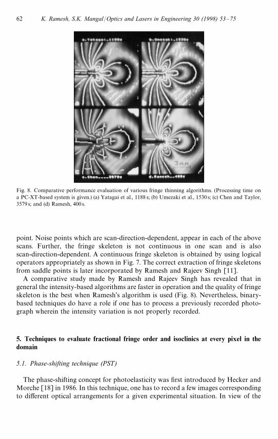
Fig. 8. Comparative performance evaluation of various fringe thinning algorithms. (Processing time ona PC-XT-based system is given.) (a) Yatagai et al., 1188 s; (b) Umezaki et al., 1530 s; (c) Chen and Taylor,3579 s; and (d) Ramesh, 400 s.

point. Noise points which are scan-direction-dependent, appear in each of the abovescans. Further, the fringe skeleton is not continuous in one scan and is alsoscan-direction-dependent. A continuous fringe skeleton is obtained by using logicaloperators appropriately as shown in Fig. 7. The correct extraction of fringe skeletonsfrom saddle points is later incorporated by Ramesh and Rajeev Singh [11].

A comparative study made by Ramesh and Rajeev Singh has revealed that ingeneral the intensity-based algorithms are faster in operation and the quality of fringeskeleton is the best when Ramesh’s algorithm is used (Fig. 8). Nevertheless, binary-based techniques do have a role if one has to process a previously recorded photo-graph wherein the intensity variation is not properly recorded.

5. Techniques to evaluate fractional fringe order and isoclinics at every pixel in thedomain

5.1. Phase-shifting technique (PST)

The phase-shifting concept for photoelasticity was first introduced by Hecker andMorche [18] in 1986. In this technique, one has to record a few images correspondingto different optical arrangements for a given experimental situation. In view of the


specific phase shifts introduced by the optical elements between the recorded images itis known as phase-shifting technique. Extending the work of Hecker and Morche,Patterson and Wang [19] reported in 1991 a technique for evaluating both isochro-matics and isoclinics using a circular polariscope. The optical arrangement used bythem is shown in Fig. 4. They included the background light intensity i

"also as

a variable and Eq. (2) is modified as

i"i"#

i!2#

i!2

[sin 2(b!/) cos d!sin 2(h!/) cos 2(b!/) sin d] (10)

substituting i."i

"#i

!/2 and i

7"i

!/2 one gets

i"i.#i

7[sin 2(b!/) cos d!sin2(h!/) cos 2(b!/) sin d] (11)

For six different positions of the II quarter-wave plate and analyser combinationthe intensity equations are summarised in Table 1. Using these, fractional retardationand the isoclinic angle are determined as follows:

d"tan~1J(i

5!i

3)2#(i

4!i

6)2

(i1!i

2) (12)

h"1

2tan~1 A

i5!i

3i4!i

6B (13)

In 1992, Sarma et al. [21] reported a methodology using a plane polariscope thatmakes use of the intensity data for three analyzer [b"0, 45 and 90°; Eq. (5)]. Theyobtained expression for fractional fringe order as inverse cosine function and isoclinicangle as inverse tangent function for the entire field. In view of the inverse cosinefunction used in the calculation of partial fringe order, there is ambiguity in determin-ing its correct sign. In view of this it reduces to a point by point technique.

Later in 1993, Asundi [22] reported a new methodology, who extended theTardy method of compensation from a point to point approach to evaluate thefractional fringe order on all points lying on the isoclinic line. Ramesh and

Table 1Intensity equations for various optical arrangements used in the phase-shifting algorithm

No. II quarter Analyser Intensity equation Fringe patternwave plate / angle b interpretation

1 0 n/4 i1"i

.#i

7cos d Circular polariscope

bright field2 0 3n/4 i

2"i

.!i

7cos d Circular polariscope

dark field3 0 0 i

3"i

.!i

7sin 2h sin d None

4 n/4 n/4 i4"i

.#i

7cos 2h sin d None

5 n/2 n/2 i5"i

.#i

7sin 2h sin d None

6 3n/4 3n/4 i6"i

.!i

7cos 2h sin d None


Ganapathy [23] have shown that among all these techniques, the algorithm ofPatterson and Wang is truly a whole field technique. The study by Haakeet al. [20] showed the applicability of the methodology of Patterson and Wang toa variety of practical problems. Patterson et al. [45] later discussed how to account forthe hardware errors introduced in the analysis.

5.2. Phase-shifting in colour domain

In this technique, the images needed for phase-shifting are recorded in colour.For quantitative data extraction green channel of the colour images are used. Rameshand Deshmukh [34] experimentally showed that for the colour camera, TMC-76(PULNiX), connected to a Matrox MVP-AT system, the green channel can bethought of to behave like a narrow-band filter. Later, Ramesh and Mangal [35]extended the technique for reflection photoelasticity using a Sony Hi8 CCD-TR750EHandycam (PAL compatible) connected to Matrox Marvel system. Since the imagesare recorded in colour domain the technique is called as phase shifting in colourdomain.

Generally, a colour camera has three filters, which have peak response to the meanwavelengths. For the purpose of standardisation, the CIE (Commission Internationalede l’Eclairage — the International Commission on Illumination) designated in 1931,the following specific wavelength values to the three primary colours as, 435.8,546.1 nm, 700.0 nm for blue, green and red, respectively [46].

Figure 9 shows the dark-field colour image of a disk under diametral compression(recorded using Sony Handycam) separated into three primary channels. The materialstress fringe value corresponding to these channels using Fig. 9 are initially obtainedand using these equivalent wavelengths for each channel is obtained and are shown inTable 2. The table shows that among the three channels, only for the green channel,the experimentally calculated wavelength is very close to the theoretical one. In viewof this, the G-plane image can be considered equivalent to an image recorded bya green filter. Further, from Fig. 9b, it is seen that the visual quality of the greenchannel is good.

5.3. Fourier transform technique

Quan et al. [25] have shown that by using carrier fringes and operating inthe frequency domain, it is possible to evaluate the fractional fringe orders usingonly one photograph. They introduced a quartz wedge between the I quarter-waveplate and the model which provide a carrier fringe with a spatial frequency off (3 lines/mm) in the x-direction. Let the retardation introduced by the wedgefor a particular point in the model be d

1, then the intensity of light transmitted is

obtained as [25]

i"i! Csin2 A

d!d1

2 B sin2 h#sin2 Ad#d

12 B cos2 hD (14)


Fig. 9. Split up of channels of the colour image of disk under diametral compression taken in reflectionarrangement using SONY Handycam (a) R-channel, (b) G-channel and (c) B-channel.

Table 2Equivalent wavelengths computed for the RGB planes

No. j [46] j(TMC-76 PULNiX CCD j (Sony Hi8 CCD-TR750Ecamera with Matrox handycam with Matrox Marval)MVP-AT system)

1 Red, 700.00 nm 598.1 nm 485.66 nm2 Green, 546.1 nm 551.9 nm 542.34 nm3 Blue, 435.8 nm 445.7 nm 546.11 nm

Fourier transform is obtained for every horizontal line in the image and the relativeretardation is obtained from the ratio of the real and imaginary part of the FT. Totalfringe orders are then obtained by phase unwrapping.

Morimoto et al. [24] used the Fourier transform technique to separate isochro-matics and the isoclinics from 90 images recorded in steps of 1° from !45 to 44° ofthe crossed plane polariscope’s analyser position. The respective intensity equationcan be obtained by modifying Eq. (6) and is

i"i!Csin2 2(h!b) sin2

d2D (15)


They obtained the Fourier transform in the b direction and showed thatin the frequency domain, u"0 corresponds to isochromatics. The direction ofprincipal stress in the whole domain is obtained by taking the arctangent of theratios of the imaginary parts and the real parts of the data in the frequencyat u"!u

0.

6. Techniques for direct evaluation of total fringe order

6.1. Spectral content analysis (SCA)

Redner [26] initially proposed in 1985 the use of spectral content from photoelasticexperiments to determine the fringe order. He concluded that SCA cannot be used toeasure small amounts of birefringence and the use of narrow-bandwidth detectorsyield multiple solutions for the fringe order. Sanford and Iyengar [27] conductedfurther studies in 1986 and showed that if the effective window is taken in the analysis,one can evaluate lower level of birefringence uniquely. Sanford [28] had made anexperimental verification of his SCA model. Voloshin and Redner [29] came up witha commercial equipment based on SCA. Haake and Patterson [30] have applied SCAto find the fringe order in stress frozen photoelastic models containing both high andlow fringe orders.

Spectral content analysis (SCA) is based on the premise that each fringe order hasa distinct spectral signature. For each data point, the transmission spectrum asa function of wavelength is experimentally obtained. Theoretical equation has beendeveloped for transmission spectrum as a function of total fringe order. In theexpression for intensity of light transmitted, the retardation, d is replaced by the totalfringe order N using stress-optic law:

N"

d2n

"

t

Fp(p

1!p

2) (16)

Since, N is also a function of wavelength, to account for dispersion one has to use

N"

N3%&

Fp3%&

Fp(17)

A polariscope is normally constructed with quarter-wave plates meant for aspecific wavelength, while white light is used, the quarter-wave plate no longerprovides a phase shift of n/2 for all wavelengths and in general behaves like a retarder.If the reference wavelength is, say k

3%&, the error introduced for all other wavelengths

(j) is

e"n2 A

jj3%&

!1B (18)

Referring to Fig. 4 and keeping the angle /"45° and b"0°, and considering thequarter-wave plate as a retarder with the retardation (n/2#e), the intensity of light


transmitted for dark and bright fields are, respectively, as

I$"i

!sin2 A

nN3%&

Fp3%&

Fp B [1!cos2 2h sin2 e] (19)

Il"i!Gcos2A

nN3%&

Fp3%&

Fp B (1!cos2 2h sin2e)#cos2 2h sin2 eH (20)

Comparing Eqs. (19) and (4), the role of quarter-wave plate error in a dark-fieldarrangement, can be modelled as a multiplication term [1!cos2 2h sin2e]. Sanforderroneously extended this to light-field arrangement too. However, Eq. (20) showsthat one also requires an additional term to correctly account for the quarter-waveplate error. This was first brought into focus by Ajovalasit et al. [47] References [28],[30] and [36] have used light-field arrangement for SCA with incorrectly modelledintensity equation to account for the quarter-wave plate error.

The value of fringe order in the theoretical equation is iteratively changed until thetheoretical and experimental curves are close in a least-squares sense. Though in SCAliterature, it is emphasised that total fringe order is determined independent of theisoclinic angle, in view of the quarter-wave plate error, it depends on the isoclinicangle h. The quarter-wave plate error in dark-field arrangement, for specificwavelengths is plotted in Fig. 10 with the reference wave length as 590 nm. However,in the literature an approximation is made and the cos2 2h term is replaced by 0.5 (i.e.h"22.5°).

The system used by Sanford [28] utilizes thermoelectrically cooled detector arraywith 256 active elements over the range of 390—730 nm. Voloshin and Redner [29]used 16 photodiode to obtain the experimental spectrum, which are obtained atintervals of 21.7 nm. Haake and Patterson [30] developed a highly sensitive instru-ment using a photomultiplier tube as a detector. The resolution of the plot can bevaried from 0.25 to 10 nm in a range of 200—900 nm. Carazo-Alvarez et al. [36]compared the use of collecting experimental data in steps of 5 and also 40 nm. Theyestablished that collecting data at 40 nm interval is reasonably accurate for problemswhere fringe order gradient is less than 1.4 fringes/mm. Extending this idea, Haakeand Patterson [31] proposed a new approach wherein the use of a B&W CCD camerain conjunction with eight high-quality optical filters corresponding to wavelengths of450, 470, 530, 590, 610, 650, 690 and 730 nm were used. This has made the methodwhole field and can be termed as digital spectral content analysis (DSCA).

6.2. Three fringe photoelasticity (TFP)

Ajovalasit et al. [32] used the RGB values of the colour image to identify the totalfringe order and termed the technique as RGB photoelasticity (RGBP). They useda hardware which can distinguish only 32 different shades for each colour plane.Ramesh and Deshmukh [33] independently proposed a technique that utilises theRGB values for total fringe order determination and termed the technique as threefringe photoelasticity (TFP) as beyond three fringes the colours tend to merge. Thehardware used by them can detect 256 shades for each colour plane.


Fig. 10. Quarter-wave plate error (1!cos2 2h sin2e) in dark-field arrangement with the reference wavelength 590 nm.

In TFP/RGBP, one has to compare the RGB values of a point with the calibratedRGB values assigned with known fringe orders so as to determine the fringe order ata given data point. The calibration table containing RGB values associated withknown fringe orders is prepared using a beam under four point bending.

Ideally, RGB values have to be unique for any fringe order. However, in view ofexperimental difficulties, the RGB values corresponding to a data point may notexactly coincide with the RGB values in the calibration table. For any test data point,an error term ‘e’ is defined as

e"(R%!R

#)2#(G

%!G

#)2#(B

%!B

#)2 (21)

where, subscript ‘e’ refers to the experimentally measured values for the data point and‘c’ denotes the values in the calibration table.

To account for the quarter-wave plate error, Ajovalasit et al. [32] suggested thatcalibration table be obtained corresponding to the isoclinic angle of 22)5°. Rameshand Deshmukh, to account for the influence of fringe gradient, suggested the genera-tion of three tables corresponding to 0—1, 0—2 and 0—3 fringe order ranges. They alsoperformed a systematic study in reducing the error in the analysis. The study hasrevealed that instead of directly using RGB values corresponding to a dark-fieldimage, if the difference of RGB values between bright- and dark-field images is used,the number of noise points is less. This is because the technique accounts for thenon-uniform illumination. The noise points are further reduced if in (bright—dark)combination, (R-G), G and B are used in Eq. (21) rather than simply RGB. Fig. 11shows the fringe order variation obtained for the disk under diametral compressionusing dark-field table, bright—dark table with combination of (R-G), G, B and the


Fig. 11. Fringe order variation for disk under diametral compression (a) using dark-field table, (b)bright—dark field table with combination of (R-G), G and B and (c) after noise removal.

fringe order variation after noise removal. The method proposed is very simple andeasy to implement. Unlike SCA, the computational demand is almost negligible andhence, is easily adaptable for devising automatic polariscopes.

7. Hybrid techniques

In PST and FT techniques to find the absolute fringe order at any point, one needsthe total fringe order for at least one point in the fringe field to be supplied by auxiliary


Fig. 11. Continued.

means. Carazo-Alvarez et al. [36] used SCA to determine total fringe order at just onepoint in the fringe field which is used as an input to unwrap the phases obtained byPST. The disadvantage of their approach is that one requires two different hardwaresone for SCA and the other for phase-shifting. PST is easily accomplished by integrat-ing an image processing system with the polariscope. But for SCA, one needsspecialised hardware such as spectral analyser, fibre-optic cables, rotating diffractiongrating, etc. It is also technically feasible to combine DSCA and PST. Though iteliminates the use of two different hardwares, DSCA involves use of eight opticalfilters and thus a cumbersome procedure.

In the methodology of PST in colour domain, colour images are recorded initially.Out of these, the first two images correspond to conventional bright- and dark-fieldarrangements (Table 1). Hence, TFP can be performed without requiring any addi-tional data. Thus, a fully automated methodology for photoelastic data acquisition ofboth isochromatic and isoclinic data is possible by combining TFP and PST in colourdomain. The advantage of the approach is that no specialised hardware other thana general-purpose colour image processing system is required. Further, since themethodology also records the whole-field fringe patterns in colour, one always hassufficient data to verify the results provided by the automated methodology.

8. Discussion

Each of the techniques reported in this paper has a particular domain of applica-tion. For example, fringe multiplication techniques come in handy to qualitativelycomment on the stress field by making visible several fringe orders. Fringe thinningtechniques do not require the calibration of the polariscope-model system and are


applicable to previously recorded photographs. Since only one photograph is neededfor the data extraction they are applicable for dynamic studies. If the intensityvariation of the fringe field recorded is reasonably well then one can use the work ofRamesh and Kelkar [39, 40] for determining fringe gradient direction to facilitatefringe ordering. For the conventional model materials, HFP is not desirable as theproblems associated with residual stress affect the results. HFP is ideal for analysingthose situations where the problem is modelled using materials that have low opticalsensitivity such as glass. Evaluation of both isochromatics and isoclinics (with somerestriction) [45] is possible for the entire field with phase-shifting techniques. Amongthese, the algorithm of Patterson and Wang [19] stand out as a truly whole fieldtechnique. Since, six images are needed, the technique is applicable only for staticproblems and widely used to analyse stress frozen slices. The accuracy achievable is$0.75° for isoclinic and $0.007 fringes for isochromatics [20]. Patterson et al. [45]conducted an error analysis and considered the perpendicularity, angular orientationand mismatch of the quarter-wave plate with the chosen wavelength. Among these,the error introduced by the mismatch of the quarter-wave plate is the highest and isreported that if the mismatch is 100 nm, the error in isochromatic value is less than0.05 fringe orders. The difficulty of PST in measuring fringe order near stressconcentration zone is reported by several investigators. Ramesh and Kelkar pointedout that the model becomes more transparent in the stress concentration zone due tothe presence of 4% of another wave length of 589.6 nm while using sodium vapoursource. This is not accounted for by the existing algorithms. Further research on PSTmust be concentrated on this aspect.

SCA is essentially a point by point technique and yields very accurate results of theorder of $0.005 fringe orders, if a photomultiplier tube is used as a sensor [30]. Theprocedure requires elaborate calibration and the result is obtained iteratively. Thebasic procedure reported by Sanford [28] is for measuring isochromatics. However,a variation to measure isoclinic is also proposed [48]. The inherent fringe gradientsensitivity of SCA is higher than PST. However, by using appropriate optical magnifi-cation, the sensitivity of PST to fringe gradient can be improved. The point by pointversion of SCA has found application in monitoring the processing of birefringentlysensitive polymers. The whole field version of SCA by Haake and Patterson [31] isnot very accurate. Hence, as a general purpose stress analysis tool it is not veryattractive. One of the significant developments of SCA is the better understanding ofa polariscope equipped with a white light. The intensity equation developed accu-rately models the dispersion of birefringence and models the mismatch of the quarterwave plate only satisfactorily. This emphasises the need of using achromatic quarter-wave plate for photoelastic analysis [49]. The knowledge of finding intensity equationdue to the presence of various wavelengths could be extended for improving PST toextract fringe data better in stress concentration zones. Fourier transform techniquesin general are highly computationally intensive. The technique of Quan et al. [25] isthe only one available to process fringe patterns from dynamic experiment. However,the technique is limited by the availability of high-density carrier fringes. The tech-nique proposed by Morimotto et al. [24] requires a whopping 90 images for process-ing. Nevertheless, the technique can give both isochromatics and isoclinics.


It is recommended in Ref. [34] that for photoelastic experiment it is desirable thatcolour fringe patterns are recorded as a part of the experimental procedure so that itprovides sufficient information to check the automated procedure if need be. The needfor using white light as a source for acquiring isoclinic without discontinuity in theentire domain is emphasised by Patterson et al. [45] The applicability of PST incolour domain to reflection photoelasticity is shown by Ramesh and Mangal [35].TFP is nothing but the extension of HFP to colour domain. The accuracy attainable[33] by TFP in the 0—1 fringe range is 0.012 fringe, 0.017 in 1—2 and 0.026 in 2—3 fringeorder range and is very attractive as a general purpose analysis using conventionalmodel materials. Knowledge of SCA has helped in accounting for the error in TFP.Ajovalasit et al. [32] proposed that if the calibration tables are obtained for isoclinicangle of 22.5°, then the results are better. Here again the use of achromatic quarter-wave plate is desirable.

9. Conclusions

A large class of problems such as determination of stress concentration factor(SCF), stress intensity factor (SIF) and also evaluation of contact stress parametersrequire only the information of isochromatic fringe orders from the field. For severalproblems in which an evaluation is to be made between different designs, it is enoughif one knows the isochromatic fringe order. In problems involving stress wavepropagation, crack propagation, etc., the exposure time for recording such phe-nomena is very short of the order of 0.5 ls. In such cases only bright-field isochro-matics are recorded and quantitative information has to be extracted by processingthe fringe field. In view of this, it is justifiable that in the literature more attention hasbeen paid to determine isochromatic fringe order. Only in special cases where one isinterested in determining individual components of stress tensor, one requires bothisochromatic fringe orders and isoclinic fringe orders. From an engineering pointof view, digital photoelasticity is a viable tool now. Since, each technique hasa particular domain of application, it is necessary to have a comprehensive softwareplatform [50].

In most of the techniques, calibration of the polariscope-model system is essential.In general SCA provides an higher level of accuracy than PST. The level of accuracyin PST can be improved by using a highly monochromatic source of light andsensitivity for higher fringe gradient is possible by using appropriate optical magnifi-cation. The accuracy in SCA can be improved by using achromatic quarter wave plateto record intensity spectra and also using a fine beam of light. It is reported thata 0.2 mm diameter beam is found to be sufficient for most analysis. For whole fieldanalysis PST is promising and for point by point analysis SCA is better. Furtherdevelopment in Fourier transform techniques is needed for its use. Though severalpapers have reported computerised and automated techniques none of them are fullyautomated in the true sense. One may require to give fringe order interactively oratleast an intelligent guess as in SCA. Full automation is possible only when onethinks of hybrid techniques. The combination of TFP with PST in colour domain is


promising to become a completely automated engineering technique with a level ofcomputation which is reasonably small.

The techniques reported so far are primarily concerned with transmission photo-elastic analysis. To an extent, the techniques have been extended to reflectionphotoelasticity too. From an engineering standpoint PST is attractive. Though it isshown to be successful for analysing stress frozen slices, the inherent contradictions inthe conventional stress freezing and slicing [51] is not overcome. Further researchmust pay attention on this aspect and PST is ideal for determining characteristicsparameters [52] too and work is currently underway in this direction.

In conventional photography in view of the use of high-resolution films for record-ing, if a fringe pattern is recorded with a particular magnification, by post-processing,any zone of the fringe field can be analysed later. However, in digital photoelasticitycertain amount of information is lost in high stress gradient zones due to digitisation.Hence, one should know a priori which zone of the fringe field is important. Anexpensive remedy is to use a very high-resolution digital camera. An economicalapproach would be to record a few images with different optical magnifications anddevelop a cascading algorithm to combine these images for interpretation.

Acknowledgements

This research was sponsored in part (Project No. 919) by the Aeronautics Researchand Development Board of the Government of India and the Department of Mechan-ical Engineering IIT Kanpur. The authors thank Prof. B. Dattaguru, Prof. K. Rajaiahand Prof. N. S. Venkataraman for their interest in this work. The second authoracknowledges the support he received from Q.I.P., Govt. of India to enable him to dothis research.

References

[1] Patterson EA. Automated photoelastic analysis. Strain 1988;24(1):15—20.[2] Muller RK, Saackel LR. Complete automatic analysis of photoelastic fringes. Exptl. Mech.

1979;19(7):245—52.[3] Seguchi Y, Tomita T, Watanabe M. Computer aided fringe pattern analyser — a case of photoelastic

fringes. Exp. Mech. 1979;19(10):362—70.[4] Chen TY, Taylor CE. Computerized fringe analysis in photomechanics. Exp. Mech.

1989;29(3):323—29.[5] Yatagai T, Nakadate S, Idesawa M, Saito H. Automatic fringe analysis using digital image processing

techniques. Opt. Engng 1982;21(3):432—35.[6] Gillies AC. Image processing approach to fringe patterns. Opt. Engng 1988;27(10):861—66.[7] Umezaki E, Tamakai T, Takahashi S. Automatic stress analysis of photoelastic experiment by use of

image processing. Exp. Tech. 1989;13(6):22—7.[8] Ramesh K, Ganesan VR, Mullick SK. Digital image processing of photoelastic fringes — a new

approach, Exp. Tech. 1991;15(5):41—6.[9] Ramesh K, Pramod BR. Digital image processing of fringe patterns in photomechanics. Opt. Engng

1992;31(7):1487—98.[10] Ramesh K, Pramod BR. A new fringe thinning algorithm in photomechanics. Proc. of VII Int. Conf.

on Experimental Mechanics, Las Vegas, USA, 8—11 June 1992:1517—23.


[11] Ramesh K, Singh RK. Comparative performance evaluation of various fringe thinning algorithms inphotomechanics. J. Electron. Imaging 1995;4(1):71—83.

[12] Yao JY. Digital image processing and isoclinics. Exp. Mech. 1990;30(3):264—9.[13] Toh SL, Tang SH, Hovanesian JD. Computerized photoelastic fringe multiplication. Exp. Tech.

1990;14(4):21—3.[14] Liu X, Yu Q. Some improvement on digital fringe-multiplication methods. Exp. Tech.

1993;17(1):26—9.[15] Chen TY. Digital fringe multiplication of photoelastic images — a new approach. Exp. Tech.

1994;18(2):15—8.[16] Chen TY. Digital fringe multiplication in three dimensional photoelasticity. J. Strain Anal. Engng

Des. 1995;30(1):1—8.[17] Voloshin AS, Burger CP. Half fringe photoelasticity — a new approach to whole field stress analysis.

Exp. Mech. 1983;23(9):304—14.[18] Hecker FW, Morche B. Computer-aided measurement of relative retardations in plane photoelastic-

ity. In: Wieringa H, editor. Experimental Stress Analysis. The Netherlands: Marhinus Nijhoffpublishers/Dordrecht, 1986:535—42.

[19] Patterson EA, Wang ZF. Towards full field automated photoelastic analysis of complex components.Strain 1991;27(2):49—56.

[20] Haake SJ, Wang ZF, Patterson EA. Evaluation of full field automated photoelastic analysis based onphase stepping. Exp. Tech. 1993;17(6):19—25.

[21] Sarma AVSSSR, Pillai SA, Subramanian G, Varadan TK. Computerized image processing forwhole-field determination of isoclinics and isochromatics. Exp. Mech. 1992;32(1):24—9.

[22] Asundi A. Phase shifting in photoelasticity. Exp. Tech. 1993;17(1):19—23.[23] Ramesh K, Ganapathy V. Phase-shifting methodologies in photoelastic analysis — the application of

Jones calculus. J. Strain Anal. Engng Des. 1996; 31(6):423—32.[24] Morimoto Y, Morimoto Jr, Y, Hayashi T. Separation of isochromatics and isoclinics using fourier

transform. Exp. Tech. 1994;18(5):13—7.[25] Quan C, Bryanston-Cross PJ. Judge TR. Photoelasticity stress analysis using carrier and FFT

techniques. Opt. Lasers Engng 1993;18:79—108.[26] Redner AS. Photoelastic measurements by means of computer-assisted spectral content analysis. Exp.

Mech. 1985;25(2):148—53.[27] Sanford RJ, Iyengar V. The measurement of the complete photoelastic fringe order using a spectral

scanner. Proc. SEM Spring Conf. on Experimental Mechanics 1985:160—8.[28] Sanford RJ. On the range and accuracy of spectrally scanned white light photoelasticity. Proc. SEM

Spring Conf. on Experimental Mechanics 1986:901—8.[29] Voloshin AS, Redner AS. Automated measurement of birefringence: development and experimental

evaluation of the techniques. Exp. Mech. 1989;29(3):252—7.[30] Haake SJ, Patterson EA. Photoelastic analysis of frozen stressed specimens using spectral-content

analysis. Exp. Mech. 1992;32(3):266—72.[31] Haake SJ, Patterson EA. Photoelastic analysis using automated polariscopes. Proc. Int. Conf. on

Mechanics of Solids and Materials Engineering (MSME 95), Singapore, 6—8 June 1995:884—8.[32] Ajovalasit A, Barone S, Petrucci G. Towards RGB photoelasticity: full-field automated photoelastic-

ity in white light. Exp. Mech. 1995;35(3):193—200.[33] Ramesh K, Deshmukh SS. Three fringe photoelasticity — use of colour image processing hardware to

automate ordering of isochromatics. Strain 1996;32(3):79—86.[34] Ramesh K, Deshmukh SS. Automation of white light photoelasticity by phase-shifting technique

using colour image processing hardware. Opt. Lasers Engng 1997;28(1):47—60.[35] Ramesh K, Mangal SK. Automation of data acquisition in reflection photoelasticity by phase shifting

methodology. Strain 1997;33(3):95—100.[36] Carazo-Alvarez J, Haake SJ, Patterson EA. Completely automated photoelastic fringe analysis. Opt.

Lasers Engng 1994;21:133—49.[37] Ramesh K. PHOTOSOFT—H: A comprehensive photoelasticity simulation module to teach the

technique of photoelasticity. Int. J. Mech. Engng Education 1997;25(4):306—24.[38] Friedrich G. Calibration of equidensity lines. Strain 1976;12:140—3.


[39] Ramesh K, Kelkar AA. Automatic ordering of isochromatic fringes — a new methodology. Strain1995;31(3):95—9.

[40] Ramesh K, Kelkar AA. Automatic fringe ordering of photoelastic fringes — a new methodology.Proc. Int. Conf. on Mechanics of Solids and materials Engineering (MSME 95), Singapore, 6—8 June1995:895—900.

[41] Srinath LS, Raghavan MR, Lingaiah K, Gargesha G, Pant B, Ramachandra K. Experimental StressAnalysis. Tata McGraw-Hill, New Delhi, 1984.

[42] Wang WC, Chen Tl. Half-fringe photoelastic determination of opening mode stress intensity factorfor edge cracked strips. Engng Fracture Mech. 1989;32(1):111—22.

[43] Voloshin AS, Burger CP. Half fringe photoelasticity for orthotropic materials. Fibre Sci. Technol.1984;21(4):341—51.

[44] Burger CP. New approach to optical methods in experimental solid mechanics through digital imageprocessing. Proc. VI Intl. Conf. Experimental Mechanics, Portland, OR, 6—10 June 1988:655—60.

[45] Patterson EA, Ji W, Wang ZF. On image analysis for birefringence measurement in photoelasticity.Opt. Lasers Engng 1997;28(1):17—36.

[46] Gonzalez RC, Woods RE. Digital Image Processing. Addison-Wesley, Reading, MA, 1993.[47] Ajovalasit A, Barone S, Petrucci G. Automated photoelasticity in white light: influence of quarter-

wave plates. J. Strain Anal. Engng Des. 1995;30(1):29—34.[48] Wang ZF, Patterson EA. Use of phase-stepping with the demodulation and fuzzy sets for birefrin-

gence measurement. Opt. Lasers Engng 1995;22:91—104.[49] Hariharan P. Achromatic and apochromatic halfwave and quarterwave retarders. Opt. Engng

1996;35(11):3335—7.[50] Ramesh K, Govindarajan R. Development of a comprehensive digital image processing module for

photoelastic data acquisition. ARDB Report No. ARDB-SP-TR-97-786-01 February 1997.[51] Srinath LS, Keshavan SY. A critical analysis of the shear difference method. J. Phys. D. Appl. Phys.

1978; 8:463—79.[52] Srinath LS, Ramesh K, Ramamurti V. Determination of characteristic parameters in three dimen-

sional photoelasticity. Opt. Engng 1988;27(3):225—30.


data acquisition techniques in digital photoelasticity: a review

Documents