Data Assimilation for Updates ofDigital Terrain ModelsThomas Knudsen

TECHNICAL REPORT NO. 14

Thomas KnudsenData Assimilation for Updates of Digital Terrain Models

National Survey and Cadastre—Denmark, technical report series number 14ISBN 978-78-92107-40-4Technical ReportPublished 2011-12-18This report is available from http://www.kms.dk

Due to the use of material distributed under Creative Commons Attribution-Share Alike 3.0 Un-ported license (see Acknowledgements), this report in its entirety is distributed under the CreativeCommons Attribution-Share Alike 3.0 Unported license, as well.

Contents

1 Introduction 41.1 DK-DEM . . . . . . . . . . . . . . . . . . . . . . . . . . . . . . . . . . . . . . . . . 41.2 Scope and aim . . . . . . . . . . . . . . . . . . . . . . . . . . . . . . . . . . . . . . 41.3 Data assimilation . . . . . . . . . . . . . . . . . . . . . . . . . . . . . . . . . . . . . 5

2 Prerequisites 62.1 Introductory remarks . . . . . . . . . . . . . . . . . . . . . . . . . . . . . . . . . . . 62.2 Spatial autocovariance . . . . . . . . . . . . . . . . . . . . . . . . . . . . . . . . . . 72.3 A DEM filtering scheme . . . . . . . . . . . . . . . . . . . . . . . . . . . . . . . . . 82.4 Spatial interpolation . . . . . . . . . . . . . . . . . . . . . . . . . . . . . . . . . . . 82.5 Delaunay triangulation . . . . . . . . . . . . . . . . . . . . . . . . . . . . . . . . . . 10

3 Test site and test data 113.1 Test site location and topography . . . . . . . . . . . . . . . . . . . . . . . . . . . . 113.2 A DTM with synthetic changes: The new ground truth . . . . . . . . . . . . . . . . . 113.3 Synthetic LiDAR observations . . . . . . . . . . . . . . . . . . . . . . . . . . . . . . 11

4 Experiments 164.1 Experiment 1: Geostatistical characterization . . . . . . . . . . . . . . . . . . . . . . 164.2 Experiment 2: Updating with simple kriging . . . . . . . . . . . . . . . . . . . . . . . 184.3 Experiment 3: Handling observational noise . . . . . . . . . . . . . . . . . . . . . . 214.4 Experiment 4: Eliminating drift by draping . . . . . . . . . . . . . . . . . . . . . . . . 22

5 Outroduction 245.1 Future work . . . . . . . . . . . . . . . . . . . . . . . . . . . . . . . . . . . . . . . 245.2 Conclusion . . . . . . . . . . . . . . . . . . . . . . . . . . . . . . . . . . . . . . . . 24Acknowledgements . . . . . . . . . . . . . . . . . . . . . . . . . . . . . . . . . . . . . . 24Notes . . . . . . . . . . . . . . . . . . . . . . . . . . . . . . . . . . . . . . . . . . . . . 25Bibliography . . . . . . . . . . . . . . . . . . . . . . . . . . . . . . . . . . . . . . . . . . 25

APPENDIX 27

A Code 27A.1 Bimorphologically constrained filtering . . . . . . . . . . . . . . . . . . . . . . . . . 27A.2 A noise reduction experiment . . . . . . . . . . . . . . . . . . . . . . . . . . . . . . 29A.3 A draping experiment . . . . . . . . . . . . . . . . . . . . . . . . . . . . . . . . . . 30

3

Chapter 1

Introduction

1.1 DK-DEM

DK-DEM, the national Danish digital elevationmodel, consists of three primary products (Dalået al., 2009):

1. A gridded digital terrain model (DTM)

2. A gridded digital surface model (DSM)

3. A set of terrain contour curves

Supplementary products include a digital terrainmodel with bridges included (for orthophoto pro-duction), but specifically not the raw data (i.e.the point cloud) used for computing the grids.

The gridded models (DSM and DTM) have agrid ground sample distance (GSD) of 1.6 m (i.e.≈ 0.4 point/m2) and were based on airborne Li-DAR observations with a similar mean density.

The LiDAR data sets used were collected bythe companies BlomInfo and Scankort in thetime frame 2005–2007. So while DK-DEM wasa big improvement compared to what was avail-able prior to its introduction in 2009, it was al-ready at that time slightly dated.

For many purposes, DK-DEM is still perfectlyadequate, but for other purposes (most obviouslythe ones exceeding the original scope of DK-DEM) it has shown necessary to collect newdata. These data, typically collected by publicinstitutions with special tasks in limited areas,could be put to good use in the process of updat-ing DK-DEM. The aim of this report is to takesome steps towards a practical realization of justthat.

1.2 Scope and aim

Since the original point cloud data sets behindthe DK-DEM grids are not available, all updates

must be carried out by combining the existinggrids with new data, which may be either gridsor point cloud data.

A few years ago, Joachim Höhle (Höhle,2009) presented a very systematic approach toDK-DEM updates, suggesting the use of pho-togrammetric methods, systematically utilizingaerial photos already collected for mapping, togenerate new height grids with an accuracy ap-proaching that of LiDAR. These height gridswill then fully replace the existing LiDAR basedgrids.

In a sense, this report takes the opposite ap-proach to Höhle: rather than generating heightdata from sytematically collected data of oppor-tunity, we are aiming for utilizing existing heightdata, collected (in potentially non-coordinated oreven non-systematical, ways), for opportunisticupdating of the existing height model.

Combining the two approaches, we may beable to put all available data into optimum useand, not the least, gain improved insight and con-fidence in the precision and accuracy of the up-dated model.

It is not just in its approach, but also in itsscope and aim, the work presented here differsfrom that of Höhle (2009): Höhle presents andevaluates a practical study based primarily onthe use of commercial implementations of al-gorithms and methods that have been developedthrough more than a decade of research by Höhleand his colleagues in international surveying andphotogrammetry laboratories.

This report, on the other hand, presents workbased on methods for gravity data analysis, orig-inally developed and used since the 1960s by thephysical geodesy community. The applicationof these methods to elevation data is unconven-tional, so in order to further develop the methods

4

and ideas within a controlled framework, all thework presented here is based on simulated data(albeit data derived from a real DTM covering a1 km × 1 km test site).

Since the results are encouraging and the im-plementation straightforward, I hope, in futurework, to be able to follow Höhle’s example ofevaluating full scale experiments based on realworld data (cf. section 5.1).

1.3 Data assimilation

Data assimilation is a term primarily used in nu-merical weather prediction, where it covers theprocess of combining newly arrived atmosphericobservations with the current model forecast, inpreparation for the next forecast cycle. Appar-ently this has nothing to do with height models,so how did data assimilation make it into the titleof this report? For two reaons, really:

First, data assimilation in the form of op-timum interpolation is an idea for which thetime was ripe in the 1960s: Largely similar ap-proaches: optimum interpolation in dynamic me-teorology, kriging in mining engineering, andleast squares collocation in geodesy1, were pub-lished within a few years time. So the term dataassimilation hints at all these ways of integratingspatial and/or spatio-temporal observations in away that optimizes the recovery of the physical

signal (modelled as a stochastic process) behindthe data.

Second, data assimilation, ethymologicallyspeaking, hints at a process of “making sim-ilar” (to assimilate). And making data simi-lar is exactly what we need when taking theopportunistic-synergistic approach of making asmuch use as possible of whatever data that hap-pens to come our way.

Getting better data for one area does not inany way make it possible for us to say muchnew about a neighbouring area. Hence, we mustmake existing and new data fit together – makethem similar.

Sometimes we may even find that the longwavelength accuracy of the existing model maybe much better than the new data, while the newdata still have much higher accuracy at shortwavelengths. 2 This is especially the case forcorridor mapping data sets, where long, essen-tially one dimensional, areas around elongatedfeatures (power lines, railroads, highways) aremapped using just one flight line.

Hence the term data assimilation – to hint ata two way process that in one direction aims atupdating an existing model by incorporating newdata (as in a human cognitive process), and in theother direction makes the new data more similarto the existing, by propagating a splash of preju-dice/prior knowledge/existing state, to the obser-vations before incorporation.

5

Chapter 2

Prerequisites

2.1 Introductory remarks

This chapter presents some of the more impor-tant mathematical and geophysical prerequisitesfor the experiments presented in chapter 4. Thepresentation is neither extensive nor complete,it is simply a brief reminder that may be safelyskippped by readers well informed in these mat-ters.

But before skipping on to the experiments, thereader is encouraged to consider a few pointsabout updating of height models which may putthe experiments in a different perspective:

1. If we have new and “perfect” data for anarea that reveals a bias in the heights of theold model, what should we do at the borderbetween old and new data?

• Introduce the new data directly inthe model, and live with the step in-evitably introduced on the border be-tween the biased and the unbiaseddata?• Arbitrarily modify the old data near

the border to get a smooth transition?• Gradually introduce the bias of the old

data into the new data, as we get closerto the border?

2. The difference between updating and bring-ing up to date: what should be done in ar-eas where we have new data, but also knowthat these data are already outdated by evennewer developments?

3. New observations having error bars fallingentirely within the error bars of the oldmodel may actually not bring any new in-formation to the table. Do we update the

models anyway (e.g. to get a local reduc-tion of the error bars)?

4. What should we do if we get new, but tech-nically inferior data (e.g. more noisy and/orlower resolution than the existing model)for an area where we know that changeshave happened.

Any competent practitioner will have good an-swers or opinions about these questions.

But when updating a national height model weare changing an essential piece of the geospatialinfrastructure. A piece that may be in use in un-known and unexpected ways in various institu-tions. Hence, updating/changing the model maybreak existing applications in interesting, but ex-pensive and disrupting, ways.

This means that a large number of relevantstakeholders may have differing opinions on thesubject. Opinions that may even be mutually ex-clusive.

A technically simple way to deal withthis could be to operate with a conservativemodel that is only updated at predictable andagreed intervals, and a progressive model semi-automatically incorporating all available newdata, including their potential errors—BleedingEdge, Blunders Included!.

But even in the case of stakeholder consen-sus on a purely conservative model, one shouldnot underestimate the value of a process of con-tinuously integrating new data, even though theimproved model will not be distributed: in thecase of continuous integration, one gets a muchbetter feeling of the actual quality of the exist-ing model, which in turn may lead to improvedmetadata.

6

2.2 Spatial autocovariance

Spatial autocovariance (or simply spatial covari-ance) is a concept describing how well a physicalobservable is represented by a nearby measure-ment. To define the autocovariance we start fromthe variance of a set of n spatial observations zi:

C0 = ∑z2

in. (2.1)

Readers expecting a different expression are re-ferred to the note on means versus models below.

We now define the lag, d as the distance be-tween two observations. For any given d, wecompute the variance-like expression

Cd = ∑ziz j

nd(2.2)

where the sum is understood to run over all ndpairs {zi,z j} having a mutual distance of d (or,in most practical cases, a mutual distance of ap-proximately d).

Computing Cd for a range of different lags re-sults in a discrete set of numbers known as theempirical covariance. To be able to estimate thecovariance for any d, we fit a continuous modelto the discrete set.

The Hirvonen covariance model

One of the simplest and most useful covariancemodels was published by Hirvonen (1962). Hir-vonen’s model is isotropic, i.e. assuming that thecovariance is a function of distance only (whichwe also did implicitly in the description above).The Hirvonen model is defined as:

CH(d) =C0

1+(

dLd

)2 (2.3)

where C0 is the variance of the data set (equa-tion 2.1), and Ld is the lag for which the covari-ance Cd (equation 2.2) has dropped to C0/2.

C0 and Ld can both be read directly from a plotof the discrete empirical covariance values. Butbe aware that C0 and Ld are not just properties ofthe data set. They are properties of the physicalfield investigated.

Hence, one should be very sceptical if a newdata set exhibit covariance values that differmuch from the existing. In other words, estima-tion of a covariance model is a natural early stepin the acceptance check of any new data set.

A note on means versus models

In geodesy it is common practice to workon anomalies, rather than raw physical values.Anomalies (or more generically speaking: resid-uals) are computed with respect to a model, es-sentially separating the deterministic part of thesignal from the stochastic. This enables us to usethe right tool for each job: Physical reasoning forthe deterministic part, and geostatistical methodsfor the stochastic part.

When not working on anomalies, it is commonpractice to model the deterministic part of a sig-nal as the mean of the observations. Hence thewell known expression

σ2 = ∑

(zi−m)2

n−1(2.4)

for the variance of a set of n observations zi withmean value m.

When subtracting an independently deriveddeterministic model from the observations, wereally subtract something that is potentially moremeaningful than the mean (i.e. a local modelvalue, rather than a global mean).

In computations involving anomalies, the laststep is to add back the value of the appropriatedeterministic model, all in all a scheme known asthe remove-restore principle, cf. e.g. Hofmann-Wellenhof and Moritz (2006, pp. 379–381).

Hence, the implied use of the remove-restoreprinciple in equations 2.1–2.2, plays the samerole as the removal of the mean, m, in equa-tion 2.4 3.

It is, however, not uncommon to further fitand subtract a low order spatial polynomial fromthe anomalies. Essentially this amounts to mod-elling (as a low order trend surface) effects un-resolved by the deterministic reference model.Evidently, when selecting a polynomial of orderzero, this is equivalent to removing the residualmean, as in equation 2.4.

The use of n in the denominator of equa-tions 2.1–2.2, rather than the n−1 used in equa-tion 2.4, comes from the fact that n−1 signifiesthe loss of one degree of freedom by the compu-tation of the mean from the same sample usedto estimate the variance. When obtaining the“mean equivalent” from an independent model,this loss does not occur.

7

2.3 A DEM filtering scheme

When applying to heights methods that were de-veloped for use with gravity data, we must cutsome corners and cannot expect to gain the samelevel of conceptual rigor as in the original field.

In the present work, this is most evident in thecase of splitting the deterministic part of the sig-nal from the stochastic. The deterministic partis constructed from the original DTM in a mean-ingful, but openly heuristic, method dubbed Bi-morphologically Constrained Filtering (BCF).

The method is documented by a code snippetin appendix A.1, but in brief it is based on it-erative application of still wider gaussian filtersthen, for each grid point, selecting the maximumdegree of filtering still keeping the change belowa predefined threshold.

This threshold is then relaxed for singular out-liers, which we do not want to consider partof the deterministic signal. The relaxation isbased on operators from the field of mathemat-ical morphology (Haralick et al., 1987). In otherwords, the filter is constrained by both the land-scape morphology and by mathematical mor-phology. Hence, the Bimorphologically Con-strained. . . moniker.

An example of BCF in action is shown in sec-tion 4.1.

2.4 Spatial interpolation

In the experiments (chapter 4), we will needto carry out spatial interpolation in variousways. For information, we quote below (withoutderivations, but with some comments), some ofthe main results derived in the admirably clear,compact, and highly recommended lecture noteby Nielsen (2009). For a very different (butequally clear) approach, see Bourke (1999)

In general, interpolation is carried out by com-puting a weighted mean of observations in thevicinity of a point of interest (POI). Essentiallyinterpolation schemes differ only in how they de-fine vicinity, and how they assign weights.

Nearest neighbour interpolation

In nearest neighbour interpolation, the observa-tion nearest to the POI is assigned the weightw = 1. All other observations are assigned theweight w = 0.

Global mean interpolation

In global mean interpolation, all N observationsare assigned the weight w = 1/N. This alsomeans that all POIs will get the same value.

Local mean interpolation

In local mean interpolation, all n observationswithin a given search radius r of the POI, are as-signed the weight 1/n. For large values of r localmean interpolation tends toward global mean in-terpolation.

Inverse distance weighting

In inverse distance weighting, the weights areconstructed such that observations close to thePOI gets higher weights. Let di denote the dis-tance from the POI to observation number i.Then weights are assigned as:

wi =1/di

∑Nj=0 1/d j

Which is trivially generalized to weights basedon powers of the inverse distance:

wi =1/dp

i

∑Nj=0 1/dp

j(2.5)

Often p = 2 is used (inverse square distanceweighting). Presumably inspired by the inversesquare nature of gravitational and electomag-netic force fields. There is, however, nothingmagical about p = 2, so if using inverse distanceweighting, the p factor should be selected in away commensurable with the autocovariance ofthe phenomenon at hand.

For p = 0, dpi = 1 for all i, turning inverse dis-

tance weighting into global mean interpolation(or local mean if the sum is restricted to pointswithin a certain distance from the POI).

For p→∞, the weight function drops off moreand more sharply, so in this case inverse distanceweighting tends toward nearest neighbour inter-polation. For most practical purposes, p = 10 issufficiently close to infinity to make this happen.This feature arguably makes 10 one of the small-est infinities in common use!

8

Figure 2.1: The Delaunay triangulation for a set of points: no point of the set is inside the circumcircleof any triangle. Delaunay triangulations tend to avoid long skinny triangles since they maximize theminimum angle of all the angles in the triangulation.

Kriging

In kriging (named after the South African miningengineer Danie Krige), the prediction weightsare designed to result in a central estimator withminimum estimation variance. This is a crypticway to say two things.

First that since we do not know the actualvalue at the POI, we cannot know the size of theprediction error (i.e. the difference between theactual value and the predicted). But by designingthe estimator appropriately, we can make surethat the statistical expectation value of the pre-diction error is zero, i.e. that the mean error of alarge number of predictions is zero. This is whatcentral estimator means.

Second that once we have designed the esti-mator to result in zero mean prediction errors,we also want to have optimum confidence thatany individual prediction error is as small as pos-sible (we do not want to achieve a zero mean bydelicately balancing huge errors with alternatingsigns). Assuming that errors are approximatelynormally distributed, the chance of running intoa large error grows with the variance of the dis-tribution. Hence, by designing the weights to re-sult in minimum error variance, we maximize thechance that the error of any individual predictionreally is very close to zero.

To make this happen in real life, we need to es-

timate a good covariance model for the physicalfield we are studying. Having obtained a vari-ance model, we must compute variance valuesCP j for the distances between the POI and the ob-servations, and Ci j for the distances between theindividual observations. The weights can then befound by solving the set of linear equations: C11 · · · C1N

... . . . ...CN1 · · · CNN

w1

...wN

=

CP1...

CPN

(2.6)

The prediction is then given by:

Z0 =[

w1 · · · wN] Z1

...ZN

(2.7)

The prediction variance is, in turn, given by

σ20 =C0−

[w1 · · · wN

] CP1...

CPN

(2.8)

To compute the set of N weights, we need tosolve a set of N linear equations. But the pro-cessing power needed to do this is proportionalto N3, which quickly makes it prohibitively ex-pensive in computer time to solve for more thanjust a few weights.

9

As a simple example consider the ratio be-tween 53 = 125 and 33 = 27, indicating thatit takes almost 5 times as long to solve for 5weights than for 3 weights.

This means that even for moderately largecomputations, we need an efficient way to selecta small, relevant subset of observations for anyPOI at hand.

To this end, the Delaunay triangulation comesto the rescue.

2.5 Delaunay triangulation

The Delaunay triangulation was introduced bythe Russian mathematician Boris Delaunay (De-launay, 1934). Any given set of points can beorganized as a area partitioning set of triangles(see figure 2.1). The Delaunay triangulation isdefined as the (unambiguous) partitioning thatglobally maximizes the minimum angle of theentire triangulation.

For any triangle in a Delaunay triangulation,no other points than its three corner points will

be situated inside the circumcircle of those threepoints. Hence, elongated triangles are essen-tially avoided, since they correspond to exces-sively large circumcircles.

Due to its many practical uses, much effort hasbeen put into the derivation and development ofvery fast algorithms for constructing the Delau-nay triangulation. In this work, the QHULL al-gorithm (Barber et al., 1996) is used. QHULLis widely used in closed- as well as open sourcesoftware. The Triangle algorithm by JonathanShewchuk (Shewchuk, 1996) is another excel-lent implementation, but Triangle is less usedthan QHULL, arguably due to a more restrictivelicencing policy.

Once the Delaunay triangulation is con-structed for a given set of points, it is easy tofind the triangle surrounding any given POI, andhence obtain a small set of 3 observations thatmay not necessarily be the nearest neighboursof the POI, but which are close to the POI andspatially distributed in a way making them goodcandidates for a robust estimation of the valueneeded at the POI.

10

Chapter 3

Test site and test data

3.1 Test site location and to-pography

The 1 km × 1 km test site used for the exper-iments in chapter 4, is situated just northwestof the village of Vejby in Helsinge Municipality,North-Zealand (figure 3.1). The landscape of theVejby area is glacially shaped and gently undu-lating. Due to its beauty, the area was the subjectof a large number of paintings from the 1840sby the National Romantic painters J.Th.Lundbye(cf. figure 3.2) and P. C. Skovgaard (Jørgensen,1995).

The test site is characterized by relatively largeand sometimes steep, height variations. Theland use/land cover (LULC) includes hedgerows,paths, dirt roads, farms, wetlands, lakes, a smallforest, farmland, a closed down and only par-tially refilled, clay pit, and (in the northern end) acottage area from around 1960. All in all a land-scape that is not only beautiful, but also challeng-ing and hence highly interesting from a heightmodelling point of view.

To establish a well controlled framework forour DTM updating experiments, we introducesynthetic changes in the existing DTM (sec-tion 3.2), and use the modified model as the newground truth.

This ground truth is in turn used as target fora synthetic LiDAR flight (section 3.3), generatingnew synthetic observations of the changed ter-rain.

Finally, in chapter 4, we combine the origi-nal (unchanged) DTM with the new synthetic Li-DAR observations, attempting to reproduce thesynthetic ground truth.

3.2 A DTM with syntheticchanges: The newground truth

The 1 km × 1 km test area is represented by a626 × 626 grid stored in an ESRI ascii formatfile (figure 3.1). We introduce change in the formof a synthetic road spanning the grid rows num-bered 523–527 (marked in white on figure 3.1).

The “road” is constructed as follows: First weremove any across track slope by computing thecolumnwise mean of the set of 5 rows.

Then we carry out an along track gaussian fil-tering of the mean row, i.e. easing the road forthe cyclists by cutting hilltops and filling val-leys (figure 3.3). Finally the filtered mean row iscopied back into the original five rows 523–527.

The resulting grid (figure 3.4) is now consid-ered the new ground truth for the experimentalwork.

3.3 Synthetic LiDAR observa-tions

The synthetic LiDAR observations are intendedto simulate the result of a single flight strip ina corridor mapping effort, mapping a strip cen-tered on the new road. The observations are gen-erated by this little snippet of Octave code, whichnotably does not take any roll/pitch/yaw irregu-larities into account:

1% rand: uniform, randn: gaussian randomness2N = 2*100*1000;3north = 6218000 + 160 + 100*(rand (N, 1) - 0.5)4east = 694000 + 500 + 1000*(rand (N, 1) - 0.5)5z = interp2 (h.x, h.y, g, east, north);6% add gaussian noise with a variance of 5 cm7noise = sqrt (0.05) * randn (N, 1);8z += noise;

11

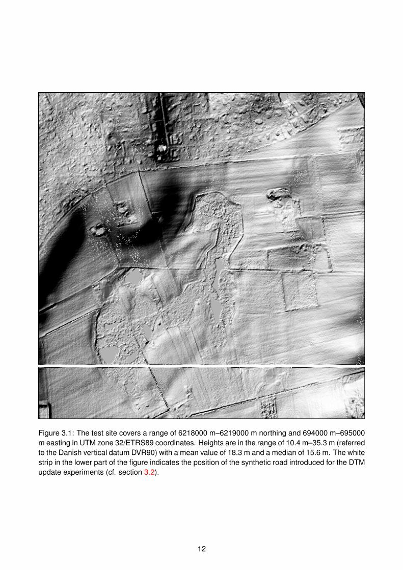
Figure 3.1: The test site covers a range of 6218000 m–6219000 m northing and 694000 m–695000m easting in UTM zone 32/ETRS89 coordinates. Heights are in the range of 10.4 m–35.3 m (referredto the Danish vertical datum DVR90) with a mean value of 18.3 m and a median of 15.6 m. The whitestrip in the lower part of the figure indicates the position of the synthetic road introduced for the DTMupdate experiments (cf. section 3.2).

12

Figure 3.2: Johan Thomas Lundbye: Landskab fra Vejby (Landscape from Vejby), 1843.

10

12

14

16

18

20

22

24

694000 694200 694400 694600 694800 695000

0

0.02

0.04

0.06

0.08

0.1

0 10 20 30 40 50 60 70 80

Figure 3.3: Left: The raw road profile (blue), and the final along track filtered road profile (black).Right: The 50 point gaussian filter used to even out the bumps in the synthetic road.

13

Figure 3.4: The final synthetic road introduced into the original grid.

14

The call to interp2 interpolates new heightvalues from the ground truth grid g.

The constants of the code snippet are to be in-terpreted as follows:

(6218000, 694000) Northing/easting ofthe lower left corner of the test site.

(160, 500) The center of the LiDAR cov-ered area is situated 160 m north and 500

m east of the loweer left corner.

(100, 1000) The flight strip is 100 m wide(north/south) and 1000 m long (east/west).

N=2*100*1000 We need 2 observations/m2

for each of the 100 m × 1000 m covered,i.e. a total of 200 000 observations.

15

Chapter 4

Experiments

4.1 Experiment 1: Geostatis-tical characterization

The first thing to do with a newly acquiredgeodetic data set is to get a general feeling ofits characteristics. For data which can be plot-ted in meaningful and straightforward ways (e.g.imagery, simple time series), plotting is the ob-vious first action. But in our case of irregularlysampled observations, a geostatistical character-ization is the obvious first action.

Actually the first step of the geostatisticalcharacterization is not geostatistical at all, butstrictly statistical (sans geo-). The first step isto plot the histogram of the data, to get an ideaof what kind of distribution is behind the data.

The upper left panel of figure 4.1 shows thehistogram for the heights of the DTM of thetest area (figure 3.1). It is not evident whatkind of distribution might fit this histogram, butit certainly isn’t a normal (Gaussian-) distribu-tion. This is even more clear from the QQ-plotin the upper right panel of figure 4.1, where thequantiles of the distribution (i.e. the lower quar-tile, median, upper quartile, and their unnamedbrothers and sisters for other values than 25%,50%, and 75% of the distribution mass) is plot-ted against the corresponding quantiles of thestandard-normal distribution (i.e. the normal dis-tribution with parameters (µ,σ2) = (0,1)). In aQQ plot, normal distributions will be depicted asa straight line, with the slope determined by theσ2 parameter, and the offset determined by the µ

parameter of the actual distribution. It is evidentfrom the QQ-plot that the distribution of the rawheights is not normal at all.

Suspecting that the non-normality is due toautocorrelation effects induced by causal (deter-ministic, non-stochastic, etc.) processes, we go

on to construct a “deterministic height surface”,as described in section 2.3, using the code pre-sented in appendix A.1. The resulting smoothsurface, and its corresponding anomalistic sur-face are shown in figure 4.2.

The histogram for the anomalies are shownin the upper left panel of figure 4.3. Despite amarked “knee” around δh= 1m and a minor wartaround δh = −1m, the histogram looks muchmore normal than the corresponding histogramfor the raw heights. The normality is confirmedby the QQ-plot in the upper right panel.

Covariances

The covariances of the raw terrain model and theanomalies, along with the corresponding Hirvo-nen covariance models, are shown in the lowerright panels of figures 4.1 and 4.3, respectively.

The first thing to note is that removing the “de-terministic height model”, really reduces bothvariance and correlation length: Where the rawDTM (with mean height removed, since it is notan anomaly, as per the discussion in section 2.2)corresponds to a Hirvonen model with parame-ters (C0,Ld) = (85 m2,182 m), the correspond-ing parameters for the anomalies are (C0,Ld) =(0.57 m2,44.8 m). In other words: by removingthe “deterministic model”, the covariance scaleis reduced by a factor of almost 150, and the cor-rellation length is reduced by a factor of morethan 4.

It is also striking how well the Hirvonen modelfits the actual data – especially in the interval[0 . . .Ld], which is really the interval we usuallywould need4.

One should, however, bear in mind that theempirical covariances in these cases are based onvery simplified computations based directly on

16

0

1

2

3

4

5

6

10 15 20 25 30 35 40

perc

enta

ge, ra

w

height

10

15

20

25

30

35

40

-6 -4 -2 0 2 4 6

em

piric

al q

ua

ntile

, ra

w

N(0,1) quantile

-0.4

-0.2

0

0.2

0.4

0.6

0.8

1

0 200 400 600 800 1000

me

an

au

toco

rre

latio

n,

raw

lag [m]

-20

0

20

40

60

80

100

0 200 400 600 800 1000

me

an

au

toco

va

ria

nce

, ra

w

lag [m]

Empirical covarianceHirvonen model (85,182)

Figure 4.1: Raw DTM geostatistics. Upper left: Histogram. Upper right: Quantile plot of dataquantiles vs. quantiles from a standard normal distribution. Lower left: Empirical autocorrelation.Lower right: Empirical autocovariance. Note that the autocorrelation only changes very slowly from1. In other words, far away points are as important as very nearby points in predicting the height atany given point.

17

Figure 4.2: Left: filtered “deterministic” terrain model. Right: corresponding anomalistic (residual)terrain model.

the gridded structure of the data: covariances arecomputed for two directions only (the directionsof the northing and easting axes), and using theboundary values of the grid as starting points.

Hence these data are based on 1252 sets of em-pirical covariance values for each of the two di-rections, each set consisting of 626 values cover-ing the lags d ∈ [0 m . . .1000 m] at steps exactlycorresponding to the grid GSD of 1.6 m.

While being a simple and totally sensible app-proach, one should expect more smooth covari-ance values than what would be the case for thethe more complex algorithm necessary for arbi-trarily distributed data.

The more complex algorithm has been usedfor preparation of figure 4.4: Here, we work on adataset consisting of 63 grid lines centered on thecenter line of the artificially introduced road (cf.section 3.2), i.e. grid line number 525. In otherwords, we work on a set of 63× 626 = 39438grid points which we in this case treat as a non-structured point cloud. Obviously, we mighthave used the synthetic LiDAR data set cover-ing the same region (cf. section 3.3), but to keepin line with the data used above, we stay with theorginal grid values.

Now, we randomly select 5 million point paircombinations and sum up their products accord-ing to equation 2.2. The sums are computedin bins of width 1.6 m, centered on the set

[1.6,3.2,4.8, . . . ,1000] (see Nielsen (2009) fordetails of the construction). In other words,rather than the almost isotropic data used above,each bin now gets contributions from point pairsat different bearings and different distances (ex-cept for the very first few bins, where only a fewcombinations of distance and bearing are possi-ble)

Not unexpected, the data in figure 4.4 lookrather more noisy than the previous plots. Alsonote that the restriction to a smaller area hasreduced both the variance and the correlationlength of the raw values as well as the anomalies.This is also as expected, as we now compare amore uniform data set (especially with respect tothe raw heights, where we now avoid the effectsof the large north–south height undulation).

4.2 Experiment 2: Updatingwith simple kriging

Figure 4.5 shows the original grid (figure 3.1),improved with data predicted using the simplekriging method described in section 2.4, and thesynthetic LiDAR data presented in section 3.3.

There really is not much to say about the re-sults: in comparison with the artificial groundtruth (figure 4.5), the most striking differencesare the (expected) effects of the noise added in

18

0

0.5

1

1.5

2

2.5

3

3.5

4

-2 -1 0 1 2 3

perc

enta

ge, anom

aly

height

-2

-1

0

1

2

3

-6 -4 -2 0 2 4 6

em

piric

al q

ua

ntile

, a

no

ma

ly

N(0,1) quantile

-0.4

-0.2

0

0.2

0.4

0.6

0.8

1

0 200 400 600 800 1000

me

an

au

toco

rre

latio

n,

an

om

aly

lag [m]

-0.2

0

0.2

0.4

0.6

0.8

0 200 400 600 800 1000

me

an

au

toco

va

ria

nce

, a

no

ma

ly

lag [m]

Empirical covarianceHirvonen model (0.57,44.8)

Figure 4.3: Anomaly DTM geostatistics. Upper left: Histogram. Upper right: Quantile plot of dataquantiles vs. quantiles from a standard normal distribution. Lower left: Empirical autocorrelation.Lower right: Empirical autocovariance. Note that the autocorrelation falls rapidly from 1. In otherwords, far away points are not as important as very nearby points in predicting the height at anygiven point.

2

4

6

8

10

12

14

0 20 40 60 80 100 120 140 160

poin

t data

covariance, gridded-e

levation

lag [m]

Empirical covarianceHirvonen model (13,109)

0

0.05

0.1

0.15

0.2

0 20 40 60 80 100 120 140 160

po

int

da

ta c

ova

ria

nce

, g

rid

de

d-a

no

ma

ly

lag [m]

Empirical covarianceHirvonen model (0.15,32)

Figure 4.4: Covariances for the narrow region around the new road. Note that the lag-axis onlycovers the first 160 m. Left: Full elevations. Right: Anomalies

19

Figure 4.5: The test site modified with updated values (computed by simple kriging) in the areaaround the artificially introduced road. The effect of the deliberately introduced noise is clearly seen.

20

Figure 4.6: Upper panel: The updated values computed by simple kriging in the area around theartificially introduced road. Centre panel: The artificial ground truth (cf. section 3.2). Lower panel:The updated values computed by simple kriging with noise reduction applied (cf. section 4.3).

the production of the synthetic LiDAR data.In the next section we will show how this noise

can be reduced. Not by filtering the gridded data,but directly as a part of the prediction process forthe updated grid values.

4.3 Experiment 3: Handlingobservational noise

Consider a height field described by a Hirvonencovariance model with the parameters (C0,Ld) =(0.5 m2,5 m), and consider the configurationshown in this sketch,

with 3 observations made at the 3 corners A,B,Cof a right triangle with side lengths a = 3, b = 4,and c = 5. Furthermore, let us place the origin ofour system at A, and the POI, P at the barycen-ter of the triangle (i.e. at the intersection of itsmedians). In this case, the code in appendix A.2,solving the simple kriging system, equation 2.6,results in the weight vector

w0 =

0.304200.293460.49874

Now consider that the observation at point Awas influenced by a noise characterized by σ2 =0.1m2. If we add that noise term to the diago-nal element for A, and solve once again for theweights, we get

wa =

0.230220.301780.53773

i.e. the weight for the noisy observation is re-duced (and so is the total sum of weights).

But what if all 3 observations were equally in-fluenced by noise? Let us add the same noiseterm to the other diagonal elements, and solveonce again for the weights:

wabc =

0.292040.298750.41855

Now, the two weights originally largest are re-duced, while the smallest weight is slightly en-larged. All in all moving the estimator more inthe direction of equal weights, which would im-prove the suppression af random noise.

In figure 4.6, we show the result of adding theartificially generated noise source (section 3.3)to the diagonal elements of equation 2.6 for anentire grid prediction experiment.

The result is quite convincing, although oneshould consider that only part of the noise reduc-tion is due to the blurring: another part is due tothe relative downweighting of the anomaly com-pared to the deterministic part.

21

One may see this as an advantage or a disad-vantage. In either case, the downweighting withrespect to the deterministic part would not hap-pen if using Ordinary Kriging (OK), rather thanSimple Kriging (SK) as used here: in OK, thesum of the weights is forced to unity, and no priorassumptions are made with respect to the meanvalue of the signal, which is implicitly reesti-mated for every prediction, hence, perhaps elim-inating the need for computing the “determinis-tic” surface.

The use of individual noise estimates for eachobservation will probably become possible asaccess to full waveform reflection data becomemore common. When that happens, includingthe noise term in the prediction process willmake even more sense.

4.4 Experiment 4: Eliminat-ing drift by draping

Airborne LiDAR observations depend heavilyon a well functioning inertial navigation system(INS) providing the pointing of the platform:The combination of position information fromthe GPS, and pointing from the INS is essentiallywhat makes it possible to convert LiDAR reflec-tion timings to ground elevations.

But INS tend to drift – a feature that can oftenbe corrected for by cross over adjustments with

neighbouring flight strips. But in the case of cor-ridor mapping, few or no neighbouring strips arerecorded. In such cases the technique of draping(cf. e.g. Strykowski and Forsberg (1998)) comeshandy. Draping builds on the assumption thatif two datasets that are supposed to have identi-cal long wavelength parts tend to drift from eachother anyway, then we must construct a correc-tion surface.

We may think of the two datasets as an old,stable but noisy model, and a newer drifting, butless noisy one.

We construct the correction surface by low-pass filtering both signals and subtracting them.The draping operation is then carried out simplyby applying the correction surface to the newerdataset.

The new dataset is then said to have beendraped over the old, inheriting the old dataset’slong wavelength accuracy, while keeping its ownhigher short wavelength accuracy.

Figure 4.7 shows a somewhat exaggerated ex-ample based on simulated data: An old terrainmodel of moderate quality (σ2 = 0.5m) is tobe updated by new data of much higher quality(σ2 = 0.05m). Unfortunately, the new data suf-fers from a huge drift of almost 8 m along the100 km track. The draping process (see code inappendix A.3) improves the RMS between the“true” landscape and the new data from a ghastly4.45 m, to the more acceptable 0.24 m

22

5

10

15

20

25

30

0 20 40 60 80 100

heig

ht [m

]

distance [km]

LdtmNobsNdtmLtrue

Corr+5

Figure 4.7: Removing drift by draping (cf. section 4.4. Except for the last 5 km, where someboundary effects become visible, the draping process is very succesful in removing the drift. Cyan:The true landscape. Blue: The old, noisy terrain model. Green: The new, less noisy but driftingobservations. Purple: The correction surface (biased by 5 m to make it fit onto the plot). Red: Thenew terrain model, consisting of the new observations (green) corrected by the correction surface(purple) / draped onto the old model (blue).

23

Chapter 5

Outroduction

5.1 Future work

The fields of geostatistics and geodesy can pro-vide plenty of useful methods and techniques forupdates of height models.

The next obvious step in the work will be touse some of the methods presented here with newreal data, rather than the simulated data used inthis report.

Other interesting work will be the (fairly sim-ple and ordinary) switch from Simple Krigingto Ordinary Kriging, with its implicit reestima-tion of the mean value for each prediction. Thismay also eliminate the need for the deterministicsurface in the predictions (while it may still beof use for visualisation and contour line genera-tion).

Also the case of non-isotropic covariancemodels, which has been left out of the scope forthis report, needs to be handled. A particularlysimple (conceptually, not implementation-wise!)example of this is the handling of breaklines bymodifying covariances for vectors crossing thebreakline.

Another interesting way of handling break-lines is through the direct inclusion of the break-line into the Delaunay triangulation (i.e. a socalled constrained Delaunay triangulation).

Finally, there is the problem of surface mod-els. In the case of surface models, we do not havea geostatistically uniform area to model. This isa significant complication, which will probablylead on to new and interesting problems!

There’s plenty of work to take up!

5.2 Conclusion

For fear of sounding too optimistic, speakingon the basis of purely synthetic data, I have re-

frained from quoting numerical results in this re-port. But the examples presented have shown tobe quite convincing.

Hence, taking the geostatistical/geodetic routeseems to be a viable option, with plenty of newopportunities that should be further explored.

Acknowledgements

Figure 2.1 was produced by Wikipedia userNü es. The original version is availablefrom http://commons.wikimedia.org/wiki/File:Delaunay_circumcircles.png, and is distributedunder the Creative Commons Attribution-ShareAlike 3.0 Unported license.

Figure 3.2 Johan Thomas Lundbye:Landskab fra Vejby (1843) was pro-vided by Wikimedia Commons (http://commons.wikimedia.org/wiki/File:Johan_Thomas_Lundbye_-_Landskab_fra_Vejby.jpg),where it was uploaded by user Rlbberlin andmarked as being “in the public domain in theUnited States, and those countries with a copy-right term of life of the author plus 100 yearsor fewer”. A somewhat better reproduction, butwith less clear reproduction right statements canbe found at the web site of the National Galleryof Denmark (Statens Museum for Kunst), http://soeg.smk.dk/VarkBillede.asp?objectid=10236.

The right triangle illustration in section 4.3was produced by Wikipedia user Gustavb(http://en.wikipedia.org/wiki/User:Gustavb).The original version is available fromhttp://en.wikipedia.org/wiki/File:Rtriangle.svg,and is distributed under the Creative CommonsAttribution-Share Alike 3.0 Unported license.

Allan Aasbjerg Nielsen, Andrew Flatman,

24

Gitte Rosenkranz, Kai Sattler, Lars Stenseng,Niels Broge, Nynne Sole Dalå and SimonLyngby Kokkendorff read and commented onthe manuscript (it goes without saying thatthe author assumes full responsibility for anyremaining errors).

My wife and kids suffered much through mymany prolonged working days during the execu-tion of this project. I am deeply grateful for theirlove, care and support.

Notes1 Least Squares Collocation is a considerably more

general framework than the other geostatistical approachesmentioned. Cf. e.g. Krarup (1969) or Hofmann-Wellenhofand Moritz (2006), chapter 10

2Although one should rather talk about precision thanaccuracy in such cases

3One should, however, never understimate the potentialfor holy wars over this issue. In this author’s totally subjec-tive, and potentially uninformed, opinion, this is probablydue to the empirical roots of statistics, making it a fruit-ful field of study and application alike—hence haunted bydomain specific practitioners, as well as more mathemat-ically inclined theorists. In discussions of (geo)statistics,these groups will often find themselves “divided by a com-mon language”.

4For exactly this reason, the parameter C0 is computeddirectly as the variance of the data, and Ld is found throughinterpolation around the first lag corresponding to a vari-ance of less than C0/2. If doing an actual least squaresfit, one would run a serious risk of putting way too muchweight on fitting the fluctuations for large lags.

References

C. Bradford Barber, David P. Dobkin, and HannuHuhdanpaa. The quickhull algorithm for con-vex hulls. ACM Trans. Math. Softw., 22:469–483, December 1996. ISSN 0098-3500. doi:http://doi.acm.org/10.1145/235815.235821.URL http://citeseerx.ist.psu.edu/viewdoc/summary?doi=10.1.1.117.405. 2.5

Paul Bourke. Interpolation methods, 1999.URL http://paulbourke.net/miscellaneous/interpolation/. 2.4

Nynne Sole Dalå, Rune Carbuhn Ander-sen, Thomas Knudsen, Simon LyngbyKokkendorff, Brian Pilemann Olsen, GitteRosenkranz, and Marianne Wind. DK-DEM:

one name—four products. In ThomasKnudsen and Brian Pilemann Olsen, editors,Proceedings of the 2nd NKG workshop onnational DEMs, Copenhagen, November,11–13 2008, number 4 in Technical ReportSeries, page 4. National Survey and Cadas-tre (KMS), Copenhagen, Denmark, 2009.URL ftp://ftp.kms.dk/download/Technical_Reports/KMS_Technical_Report_4.pdf. 1.1

B. Delaunay. Sur la sphère vide. IzvestiaAkademii Nauk SSSR, Otdelenie Matematich-eskikh i Estestvennykh Nauk, 7:793–800,1934. Here quoted from the WikiPediaarticle “Delaunay Triangulation”, http://en.wikipedia.org/wiki/Delaunay_triangulation.2.5

R. M. Haralick, S. R. Sternberg, and X. Zhuang.Image analysis using mathematical morphol-ogy. IEEE transactions on Pattern Analy-sis and Machine Intelligence, 9(4):532–550,1987. 2.3

R. A. Hirvonen. On the statistical analysis ofgravity anomalies, volume 37 of Publicationsof the Isostatic Institute of the InternationalAssociation of Geodesy. The Isostatic Instituteof the International Association of Geodesy,Helsinki, Finland, 1962. 2.2

Bernhard Hofmann-Wellenhof and HelmutMoritz. Physical Geodesy. Springer,Wien/New York, Second corrected edition,2006. 2.2, 1

Joachim Höhle. Updating of the Danish Ele-vation Model by means of photogrammetricmethods. Technical Report 3, National Sur-vey and Cadastre (KMS), Copenhagen, Den-mark, 2009. URL ftp://ftp.kms.dk/download/Technical_Reports/kmsrep_3.pdf. 1.2

Jens Anker Jørgensen. Vejby i vorehjerter. In Vejby-Tibirke årbog, page 5.Vejby-Tibirke Selskabet, 1995. URLhttp://www.vejby-tibirke-selskabet.dk/aarbog/aarbog.asp?page=33. 3.1

Torben Krarup. A contribution to the mathemati-cal foundation of physical geodesy, volume 44of Geodætisk Institut Meddelelser. GeodætiskInstitut, Copenhagen, Denmark, 1969. 1

25

A. A. Nielsen. Geostatistics and analysis of spa-tial data, oct 2009. URL http://www2.imm.dtu.dk/pubdb/p.php?5177. 2.4, 4.1

Jonathan Richard Shewchuk. Triangle: Engi-neering a 2D Quality Mesh Generator andDelaunay Triangulator. In Ming C. Lin andDinesh Manocha, editors, Applied Computa-tional Geometry: Towards Geometric Engi-neering, volume 1148 of Lecture Notes inComputer Science, pages 203–222. Springer-Verlag, May 1996. URL http://www.cs.cmu.

edu/~quake/triangle.research.html. From theFirst ACM Workshop on Applied Computa-tional Geometry. 2.5

Gabriel Strykowski and René Forsberg. Opera-tional merging of satellite, airborne and sur-face gravity data by draping techniques. InRené Forsberg, Martine Feissel, and Rein-hard Dietrich, editors, Geodesy on the Move;Gravity, Geoid, Geodynamics and Antarctica,pages 243–248. Springer Verlag, 1998. 4.4

26

Appendix A

Code

A.1 Bimorphologically constrained filtering

NOTE: this code is taken directly from the Octave input file. Some lengthy input/output operationshave been edited out, and all subroutines called have been left out from the listing, as the code isprovided for illustration only – mostly as pseudocode.

1function ret = filtering (base, cmax, padsize)2[h g] = (read header and grid data here)34kernelsizes = [3 5 7 9 11 21 41 77]5kernelvariances = [.1 .1 .1 .09 .07 .07 .04 .04]6iter = prod(size(kernelsizes))7f = zeros([size(g) iter]);89f(:,:,1) = g;1011% filter121314for i = 2:iter,15iteration = i16kernel = gaussian(kernelsizes(i), kernelvariances(i));17kernel = kernel*kernel’;18kernel /= sum(kernel(:));19f(:,:,i) = filter2 (kernel, f(:,:,i-1));20end2122% compute corrections going from filtered to plain signal23d = zeros([size(g) iter]);24for i = 2:iter,25d(:,:,i) = f(:,:,i) - g;26end2728maxd = max(d(:,:,iter)(:))29mind = min(d(:,:,iter)(:))3031% for each grid node select the filter giving maximum smoothness without excessive adjustment32% avoid some noise by morphological transformations33n = iter * ones (size (g));34c = d(:,:,iter);35for i = iter-1:-1:1,36mask = logical((c > cmax) | (c < -cmax));37mask = bwmorph(mask, ’clean’);38mask = bwmorph(mask, ’open’);3940c(mask) = d(:,:,i)(mask);41n(mask) = i;42end4344final = g+c;45464748kernel = gaussian(19, 0.1);49kernel = kernel*kernel’;

27

50kernel /= sum(kernel(:));51f = filter2 (kernel, final);5253c = f - g;54mask = logical((c > cmax) | (c < -cmax));55absolutely_final = f;56absolutely_final(mask) = final(mask);5758(write reults here)5960endfunction

28

A.2 A noise reduction experiment

This is the code referred to in section 4.312% coordinates of observations3A = [0 0];4B = [4 3];5C = [4 0];67% coordinate of the POI8P = (A+B+C)/3;910Dp = [ sqrt(sum((P-A).^2)) % distance from P to A11sqrt(sum((P-B).^2)) % distance from P to B12sqrt(sum((P-C).^2)) ]; % distance from P to C13141516Dn = [ 0 5 4 % distances from A to A, B, C175 0 3 % distances from B to A, B, C184 3 0 ]; % distances from C to A, B, C1920% Hirvonen parameters21C0 = 0.522Ld = 52324% Covariances between the observations25Cn = C0 ./ (1 + (Dn./Ld).^2)2627% Covariances between the POI and the observations28Cp = C0 ./ (1 + (Dp./Ld).^2)2930% Compute weights31w0 = Cn\Cp323334% Assume observation at A is noisy35Cn(1,1) += 0.1;3637% Compute new weights38wa = Cn\Cp3940% Assume all observations are equally noisy41Cn(2,2) += 0.1;42Cn(3,3) += 0.1;4344% Compute new weights45wabc = Cn\Cp

29

A.3 A draping experiment

This is the code referred to in section 4.4.1% true landscape 10 observations/km for 0..100 km:2X = [0:0.1:100];34Ltrue = 10 + 0.1 * X;56% existing DTM: noisy7Ldtm = Ltrue + sqrt(0.5)*randn(size(Ltrue));89% the inertial navigation system drifts slowly.10Inoise = sqrt(0.0001)*randn(size(Ltrue));11Idrift = cumsum(abs(Inoise));12max(Idrift)1314% new observations: less noisy, but drift from the INS15Nobs = Ltrue + sqrt(0.05)*randn(size(Ltrue)) + Idrift;161718% box filter kernel19B = ones(1,50)/50;2021% Filter the DTM22w = Ldtm;23% pad with boundary values to reduce boundary effects of the filtering24u = [repmat(w(1), size(w)) w repmat(w(end),size(w))];25% do a symmetric filtering to avoid pushing the signal rightwards26f1 = filter(B, 1, u)(prod(size(w))+1:2*prod(size(w)));27u = u(end:-1:1); % reverse raw signal28f2 = filter(B, 1, u)(prod(size(w))+1:2*prod(size(w)));29f2 = f2(end:-1:1); % reverse result30Fdtm = (f1+f2)/2;3132% Then filter the new observations using the same code33w = Nobs;34u = [repmat(w(1), size(w)) w repmat(w(end),size(w))];35f1 = filter(B, 1, u)(prod(size(w))+1:2*prod(size(w)));36u = u(end:-1:1);37f2 = filter(B, 1, u)(prod(size(w))+1:2*prod(size(w)));38f2 = f2(end:-1:1);39Fobs = (f1+f2)/2;4041% the correction factor is the long wavelength difference42Corr = Fobs - Fdtm;4344% remove INS drift from New OBServations, creating the New DTM45Ndtm = Nobs - Corr;4647plot (X’, [Ldtm; Nobs; Ndtm; Ltrue; Corr+5]’);48grid on;49xlabel (’distance [km]’);50ylabel (’height [m]’);51legend(’Ldtm’, ’Nobs’, ’Ndtm’, ’Ltrue’, ’Corr+5’);

30

National Survey and CadastreRentemestervej 82400 Copenhagen NV, Denmarkhttp://www.kms.dk