Data Compression

Debra A. Lelewer and Daniel S. Hirschberg

Abstract

This paper surveys a variety of data compression methods spanning almost forty years

of research, from the work of Shannon, Fano and Hu�man in the late 40's to a technique

developed in 1986. The aim of data compression is to reduce redundancy in stored or

communicated data, thus increasing e�ective data density. Data compression has important

application in the areas of �le storage and distributed systems.

Concepts from information theory, as they relate to the goals and evaluation of data

compression methods, are discussed brie y. A framework for evaluation and comparison of

methods is constructed and applied to the algorithms presented. Comparisons of both theo-

retical and empirical natures are reported and possibilities for future research are suggested.

INTRODUCTION

Data compression is often referred to as coding, where coding is a very general term

encompassing any special representation of data which satis�es a given need. Information

theory is de�ned to be the study of e�cient coding and its consequences, in the form of speed

1

of transmission and probability of error [Ingels 1971]. Data compression may be viewed as

a branch of information theory in which the primary objective is to minimize the amount

of data to be transmitted. The purpose of this paper is to present and analyze a variety of

data compression algorithms.

A simple characterization of data compression is that it involves transforming a string

of characters in some representation (such as ASCII) into a new string (of bits, for exam-

ple) which contains the same information but whose length is as small as possible. Data

compression has important application in the areas of data transmission and data storage.

Many data processing applications require storage of large volumes of data, and the number

of such applications is constantly increasing as the use of computers extends to new disci-

plines. At the same time, the proliferation of computer communication networks is resulting

in massive transfer of data over communication links. Compressing data to be stored or

transmitted reduces storage and/or communication costs. When the amount of data to be

transmitted is reduced, the e�ect is that of increasing the capacity of the communication

channel. Similarly, compressing a �le to half of its original size is equivalent to doubling the

capacity of the storage medium. It may then become feasible to store the data at a higher,

thus faster, level of the storage hierarchy and reduce the load on the input/output channels

of the computer system.

Many of the methods to be discussed in this paper are implemented in production sys-

tems. The UNIX utilities compact and compress are based on methods to be discussed in

Sections 4 and 5 respectively [UNIX 1984]. Popular �le archival systems such as ARC and

PKARC employ techniques presented in Sections 3 and 5 [ARC 1986; PKARC 1987]. The

savings achieved by data compression can be dramatic; reduction as high as 80% is not

uncommon [Reghbati 1981]. Typical values of compression provided by compact are: text

(38%), Pascal source (43%), C source (36%) and binary (19%). Compress generally achieves

better compression (50{60% for text such as source code and English), and takes less time

to compute [UNIX 1984]. Arithmetic coding (Section 3.4) has been reported to reduce a �le

to anywhere from 12.1 to 73.5% of its original size [Witten et al. 1987]. Cormack reports

that data compression programs based on Hu�man coding (Section 3.2) reduced the size of a

large student-record database by 42.1% when only some of the information was compressed.

As a consequence of this size reduction, the number of disk operations required to load the

database was reduced by 32.7% [Cormack 1985]. Data compression routines developed with

speci�c applications in mind have achieved compression factors as high as 98% [Severance

1983].

2

While coding for purposes of data security (cryptography) and codes which guarantee

a certain level of data integrity (error detection/correction) are topics worthy of attention,

these do not fall under the umbrella of data compression. With the exception of a brief

discussion of the susceptibility to error of the methods surveyed (Section 7), a discrete

noiseless channel is assumed. That is, we assume a system in which a sequence of symbols

chosen from a �nite alphabet can be transmitted from one point to another without the

possibility of error. Of course, the coding schemes described here may be combined with

data security or error correcting codes.

Much of the available literature on data compression approaches the topic from the point

of view of data transmission. As noted earlier, data compression is of value in data storage

as well. Although this discussion will be framed in the terminology of data transmission,

compression and decompression of data �les for storage is essentially the same task as sending

and receiving compressed data over a communication channel. The focus of this paper is on

algorithms for data compression; it does not deal with hardware aspects of data transmission.

The reader is referred to Cappellini for a discussion of techniques with natural hardware

implementation [Cappellini 1985].

Background concepts in the form of terminology and a model for the study of data

compression are provided in Section 1. Applications of data compression are also discussed

in Section 1, to provide motivation for the material which follows.

While the primary focus of this survey is data compression methods of general utility,

Section 2 includes examples from the literature in which ingenuity applied to domain-speci�c

problems has yielded interesting coding techniques. These techniques are referred to as

semantic dependent since they are designed to exploit the context and semantics of the

data to achieve redundancy reduction. Semantic dependent techniques include the use of

quadtrees, run length encoding, or di�erence mapping for storage and transmission of image

data [Gonzalez and Wintz 1977; Samet 1984].

General-purpose techniques, which assume no knowledge of the information content of

the data, are described in Sections 3{5. These descriptions are su�ciently detailed to provide

an understanding of the techniques. The reader will need to consult the references for

implementation details. In most cases, only worst-case analyses of the methods are feasible.

To provide a more realistic picture of their e�ectiveness, empirical data is presented in

Section 6. The susceptibility to error of the algorithms surveyed is discussed in Section 7

and possible directions for future research are considered in Section 8.

3

1. FUNDAMENTAL CONCEPTS

A brief introduction to information theory is provided in this section. The de�nitions

and assumptions necessary to a comprehensive discussion and evaluation of data compression

methods are discussed. The following string of characters is used to illustrate the concepts

de�ned: EXAMPLE = \aa bbb cccc ddddd eeeeee fffffffgggggggg".

1.1 De�nitions

A code is a mapping of source messages (words from the source alphabet �) into

codewords (words of the code alphabet �). The source messages are the basic units into

which the string to be represented is partitioned. These basic units may be single sym-

bols from the source alphabet, or they may be strings of symbols. For string EXAMPLE,

� = fa; b; c; d; e; f; g; spaceg. For purposes of explanation, � will be taken to be f0; 1g.

Codes can be categorized as block-block, block-variable, variable-block or variable-variable,

where block-block indicates that the source messages and codewords are of �xed length and

variable-variable codes map variable-length source messages into variable-length codewords.

A block-block code for EXAMPLE is shown in Figure 1.1 and a variable-variable code is

given in Figure 1.2. If the string EXAMPLE were coded using the Figure 1.1 code, the

length of the coded message would be 120; using Figure 1.2 the length would be 30.

source message codeword

a 000

b 001

c 010

d 011

e 100

f 101

g 110

space 111

Figure 1.1 A block-block code.

The oldest and most widely used codes, ASCII and EBCDIC, are examples of block-block

codes, mapping an alphabet of 64 (or 256) single characters onto 6-bit (or 8-bit) codewords.

4

source message codeword

aa 0

bbb 1

cccc 10

ddddd 11

eeeeee 100

fffffff 101

gggggggg 110

space 111

Figure 1.2 A variable-variable code.

These are not discussed, as they do not provide compression. The codes featured in this

survey are of the block-variable, variable-variable, and variable-block types.

When source messages of variable length are allowed, the question of how a message

ensemble (sequence of messages) is parsed into individual messages arises. Many of the algo-

rithms described here are de�ned-word schemes. That is, the set of source messages is deter-

mined prior to the invocation of the coding scheme. For example, in text �le processing each

character may constitute a message, or messages may be de�ned to consist of alphanumeric

and non-alphanumeric strings. In Pascal source code, each token may represent a message.

All codes involving �xed-length source messages are, by default, de�ned-word codes. In free-

parsemethods, the coding algorithm itself parses the ensemble into variable-length sequences

of symbols. Most of the known data compression methods are de�ned-word schemes; the

free-parse model di�ers in a fundamental way from the classical coding paradigm.

A code is distinct if each codeword is distinguishable from every other (i.e., the mapping

from source messages to codewords is one-to-one). A distinct code is uniquely decodable if

every codeword is identi�able when immersed in a sequence of codewords. Clearly, each of

these features is desirable. The codes of Figure 1.1 and Figure 1.2 are both distinct, but the

code of Figure 1.2 is not uniquely decodable. For example, the coded message 11 could be

decoded as either \ddddd" or \bbbbbb". A uniquely decodable code is a pre�x code (or pre�x-

free code) if it has the pre�x property, which requires that no codeword is a proper pre�x of

any other codeword. All uniquely decodable block-block and variable-block codes are pre�x

codes. The code with codewords f1; 100000; 00g is an example of a code which is uniquely

5

decodable but which does not have the pre�x property. Pre�x codes are instantaneously

decodable; that is, they have the desirable property that the coded message can be parsed

into codewords without the need for lookahead. In order to decode a message encoded using

the codeword set f1; 100000; 00g, lookahead is required. For example, the �rst codeword of

the message 1000000001 is 1, but this cannot be determined until the last (tenth) symbol of

the message is read (if the string of zeros had been of odd length, then the �rst codeword

would have been 100000).

A minimal pre�x code is a pre�x code such that if x is a proper pre�x of some codeword,

then x� is either a codeword or a proper pre�x of a codeword, for each letter � in �. The set

of codewords f00; 01; 10g is an example of a pre�x code which is not minimal. The fact that

1 is a proper pre�x of the codeword 10 requires that 11 be either a codeword or a proper

pre�x of a codeword, and it is neither. Intuitively, the minimality constraint prevents the

use of codewords which are longer than necessary. In the above example the codeword 10

could be replaced by the codeword 1, yielding a minimal pre�x code with shorter codewords.

The codes discussed in this paper are all minimal pre�x codes.

In this section, a code has been de�ned to be a mapping from a source alphabet to a

code alphabet; we now de�ne related terms. The process of transforming a source ensemble

into a coded message is coding or encoding. The encoded message may be referred to as an

encoding of the source ensemble. The algorithm which constructs the mapping and uses it

to transform the source ensemble is called the encoder. The decoder performs the inverse

operation, restoring the coded message to its original form.

1.2 Classi�cation of Methods

In addition to the categorization of data compression schemes with respect to message

and codeword lengths, these methods are classi�ed as either static or dynamic. A static

method is one in which the mapping from the set of messages to the set of codewords

is �xed before transmission begins, so that a given message is represented by the same

codeword every time it appears in the message ensemble. The classic static de�ned-word

scheme is Hu�man coding [Hu�man 1952]. In Hu�man coding, the assignment of codewords

to source messages is based on the probabilities with which the source messages appear

in the message ensemble. Messages which appear more frequently are represented by short

codewords; messages with smaller probabilities map to longer codewords. These probabilities

are determined before transmission begins. A Hu�man code for the ensemble EXAMPLE is

given in Figure 1.3. If EXAMPLE were coded using this Hu�man mapping, the length of

6

the coded message would be 117. Static Hu�man coding is discussed in Section 3.2. Other

static schemes are discussed in Sections 2 and 3.

source message probability codeword

a 2=40 1001

b 3=40 1000

c 4=40 011

d 5=40 010

e 6=40 111

f 7=40 110

g 8=40 00

space 5=40 101

Figure 1.3 A Hu�man code for the message EXAMPLE (code length=117).

A code is dynamic if the mapping from the set of messages to the set of codewords changes

over time. For example, dynamic Hu�man coding involves computing an approximation to

the probabilities of occurrence \on the y", as the ensemble is being transmitted. The

assignment of codewords to messages is based on the values of the relative frequencies of

occurrence at each point in time. A message x may be represented by a short codeword

early in the transmission because it occurs frequently at the beginning of the ensemble, even

though its probability of occurrence over the total ensemble is low. Later, when the more

probable messages begin to occur with higher frequency, the short codeword will be mapped

to one of the higher probability messages and x will be mapped to a longer codeword. As an

illustration, Figure 1.4 presents a dynamic Hu�man code table corresponding to the pre�x

\aa bbb" of EXAMPLE. Although the frequency of space over the entire message is greater

than that of b, at this point in time b has higher frequency and therefore is mapped to the

shorter codeword.

Dynamic codes are also referred to in the literature as adaptive, in that they adapt

to changes in ensemble characteristics over time. The term adaptive will be used for the

remainder of this paper; the fact that these codes adapt to changing characteristics is the

source of their appeal. Some adaptive methods adapt to changing patterns in the source

[Welch 1984] while others exploit locality of reference [Bentley et al. 1986]. Locality of

reference is the tendency, common in a wide variety of text types, for a particular word to

7

source message probability codeword

a 2=6 10

b 3=6 0

space 1=6 11

Figure 1.4 A dynamic Hu�man code table for the pre�x \aa bbb" of message EXAMPLE.

occur frequently for short periods of time then fall into disuse for long periods.

All of the adaptive methods are one-pass methods; only one scan of the ensemble is

required. Static Hu�man coding requires two passes: one pass to compute probabilities and

determine the mapping, and a second pass for transmission. Thus, as long as the encoding

and decoding times of an adaptive method are not substantially greater than those of a

static method, the fact that an initial scan is not needed implies a speed improvement in

the adaptive case. In addition, the mapping determined in the �rst pass of a static coding

scheme must be transmitted by the encoder to the decoder. The mapping may preface each

transmission (that is, each �le sent), or a single mapping may be agreed upon and used for

multiple transmissions. In one-pass methods the encoder de�nes and rede�nes the mapping

dynamically, during transmission. The decoder must de�ne and rede�ne the mapping in

sympathy, in essence \learning" the mapping as codewords are received. Adaptive methods

are discussed in Sections 4 and 5.

An algorithm may also be a hybrid, neither completely static nor completely dynamic. In

a simple hybrid scheme, sender and receiver maintain identical codebooks containing k static

codes. For each transmission, the sender must choose one of the k previously-agreed-upon

codes and inform the receiver of his choice (by transmitting �rst the \name" or number of

the chosen code). Hybrid methods are discussed further in Section 2 and Section 3.2.

1.3 A Data Compression Model

In order to discuss the relative merits of data compression techniques, a framework for

comparison must be established. There are two dimensions along which each of the schemes

discussed here may be measured, algorithm complexity and amount of compression. When

data compression is used in a data transmission application, the goal is speed. Speed of

transmission depends upon the number of bits sent, the time required for the encoder to

generate the coded message, and the time required for the decoder to recover the original

8

ensemble. In a data storage application, although the degree of compression is the primary

concern, it is nonetheless necessary that the algorithm be e�cient in order for the scheme to

be practical. For a static scheme, there are three algorithms to analyze: the map construction

algorithm, the encoding algorithm, and the decoding algorithm. For a dynamic scheme, there

are just two algorithms: the encoding algorithm, and the decoding algorithm.

Several common measures of compression have been suggested: redundancy [Shannon

and Weaver 1949], average message length [Hu�man 1952], and compression ratio [Rubin

1976; Ruth and Kreutzer 1972]. These measures are de�ned below. Related to each of these

measures are assumptions about the characteristics of the source. It is generally assumed in

information theory that all statistical parameters of a message source are known with perfect

accuracy [Gilbert 1971]. The most common model is that of a discrete memoryless source; a

source whose output is a sequence of letters (or messages), each letter being a selection from

some �xed alphabet a

1

; : : : ; a

n

. The letters are taken to be random, statistically independent

selections from the alphabet, the selection being made according to some �xed probability

assignment p(a

1

); : : : ; p(a

n

) [Gallager 1968]. Without loss of generality, the code alphabet

is assumed to be f0; 1g throughout this paper. The modi�cations necessary for larger code

alphabets are straightforward.

It is assumed that any cost associated with the code letters is uniform. This is a reason-

able assumption, although it omits applications like telegraphy where the code symbols are

of di�erent durations. The assumption is also important, since the problem of constructing

optimal codes over unequal code letter costs is a signi�cantly di�erent and more di�cult

problem. Perl et al. and Varn have developed algorithms for minimum-redundancy pre�x

coding in the case of arbitrary symbol cost and equal codeword probability [Perl et al. 1975;

Varn 1971]. The assumption of equal probabilities mitigates the di�culty presented by the

variable symbol cost. For the more general unequal letter costs and unequal probabilities

model, Karp has proposed an integer linear programming approach [Karp 1961]. There have

been several approximation algorithms proposed for this more di�cult problem [Krause 1962;

Cot 1977; Mehlhorn 1980].

When data is compressed, the goal is to reduce redundancy, leaving only the informa-

tional content. The measure of information of a source message a

i

(in bits) is � lg p(a

i

) y.

This de�nition has intuitive appeal; in the case that p(a

i

) = 1, it is clear that a

i

is not

at all informative since it had to occur. Similarly, the smaller the value of p(a

i

), the more

unlikely a

i

is to appear, hence the larger its information content. The reader is referred to

y lg denotes the base 2 logarithm

9

Abramson for a longer, more elegant discussion of the legitimacy of this technical de�nition

of the concept of information [Abramson 1963, pp. 6{13]. The average information content

over the source alphabet can be computed by weighting the information content of each

source letter by its probability of occurrence, yielding the expression

P

n

i=1

[�p(a

i

) lg p(a

i

)].

This quantity is referred to as the entropy of a source letter, or the entropy of the source,

and is denoted by H. Since the length of a codeword for message a

i

must be su�cient to

carry the information content of a

i

, entropy imposes a lower bound on the number of bits

required for the coded message. The total number of bits must be at least as large as the

product of H and the length of the source ensemble. Since the value of H is generally not an

integer, variable length codewords must be used if the lower bound is to be achieved. Given

that message EXAMPLE is to be encoded one letter at a time, the entropy of its source can

be calculated using the probabilities given in Figure 1.3: H = 2.894, so that the minimum

number of bits contained in an encoding of EXAMPLE is 116. The Hu�man code given in

Section 1.2 does not quite achieve the theoretical minimum in this case.

Both of these de�nitions of information content are due to Shannon. A derivation of the

concept of entropy as it relates to information theory is presented by Shannon [Shannon and

Weaver 1949]. A simpler, more intuitive explanation of entropy is o�ered by Ash [Ash 1965].

The most common notion of a \good" code is one which is optimal in the sense of

having minimum redundancy. Redundancy can be de�ned as:

P

p(a

i

)l

i

�

P

[�p(a

i

) lg p(a

i

)]

where l

i

is the length of the codeword representing message a

i

. The expression

P

p(a

i

)l

i

represents the lengths of the codewords weighted by their probabilities of occurrence, that

is, the average codeword length. The expression

P

[�p(a

i

) lg p(a

i

)] is entropy, H. Thus,

redundancy is a measure of the di�erence between average codeword length and average

information content. If a code has minimum average codeword length for a given discrete

probability distribution, it is said to be a minimum redundancy code.

We de�ne the term local redundancy to capture the notion of redundancy caused by local

properties of a message ensemble, rather than its global characteristics. While the model

used for analyzing general-purpose coding techniques assumes a random distribution of the

source messages, this may not actually be the case. In particular applications the tendency

for messages to cluster in predictable patterns may be known. The existence of predictable

patterns may be exploited to minimize local redundancy. Examples of applications in which

local redundancy is common, and methods for dealing with local redundancy, are discussed

in Section 2 and Section 6.2.

10

Hu�man uses average message length,

P

p(a

i

)l

i

, as a measure of the e�ciency of a code.

Clearly the meaning of this term is the average length of a coded message. We will use

the term average codeword length to represent this quantity. Since redundancy is de�ned to

be average codeword length minus entropy and entropy is constant for a given probability

distribution, minimizing average codeword length minimizes redundancy.

A code is asymptotically optimal if it has the property that for a given probability dis-

tribution, the ratio of average codeword length to entropy approaches 1 as entropy tends

to in�nity. That is, asymptotic optimality guarantees that average codeword length ap-

proaches the theoretical minimum (entropy represents information content, which imposes a

lower bound on codeword length).

The amount of compression yielded by a coding scheme can be measured by a compres-

sion ratio. The term compression ratio has been de�ned in several ways. The de�nition

C = (average message length)/(average codeword length) captures the common meaning,

which is a comparison of the length of the coded message to the length of the original en-

semble [Cappellini 1985]. If we think of the characters of the ensemble EXAMPLE as 6-bit

ASCII characters, then the average message length is 6 bits. The Hu�man code of Section

1.2 represents EXAMPLE in 117 bits, or 2.9 bits per character. This yields a compression

ratio of 6/2.9, representing compression by a factor of more than 2. Alternatively, we may

say that Hu�man encoding produces a �le whose size is 49% of the original ASCII �le, or

that 49% compression has been achieved.

A somewhat di�erent de�nition of compression ratio, by Rubin, C = (S �O �OR)=S,

includes the representation of the code itself in the transmission cost [Rubin 1976]. In this

de�nition S represents the length of the source ensemble, O the length of the output (coded

message), and OR the size of the \output representation" (eg., the number of bits required

for the encoder to transmit the code mapping to the decoder). The quantity OR constitutes

a \charge" to an algorithm for transmission of information about the coding scheme. The

intention is to measure the total size of the transmission (or �le to be stored).

1.4 Motivation

As discussed in the Introduction, data compression has wide application in terms of

information storage, including representation of the abstract data type string [Standish 1980]

and �le compression. Hu�man coding is used for compression in several �le archival systems

[ARC 1986; PKARC 1987], as is Lempel-Ziv coding, one of the adaptive schemes to be

discussed in Section 5. An adaptive Hu�man coding technique is the basis for the compact

11

command of the UNIX operating system, and the UNIX compress utility employs the Lempel-

Ziv approach [UNIX 1984].

In the area of data transmission, Hu�man coding has been passed over for years in favor

of block-block codes, notably ASCII. The advantage of Hu�man coding is in the average

number of bits per character transmitted, which may be much smaller than the lg n bits

per character (where n is the source alphabet size) of a block-block system. The primary

di�culty associated with variable-length codewords is that the rate at which bits are pre-

sented to the transmission channel will uctuate, depending on the relative frequencies of

the source messages. This requires bu�ering between the source and the channel. Advances

in technology have both overcome this di�culty and contributed to the appeal of variable-

length codes. Current data networks allocate communication resources to sources on the

basis of need and provide bu�ering as part of the system. These systems require signi�cant

amounts of protocol, and �xed-length codes are quite ine�cient for applications such as

packet headers. In addition, communication costs are beginning to dominate storage and

processing costs, so that variable-length coding schemes which reduce communication costs

are attractive even if they are more complex. For these reasons, one could expect to see even

greater use of variable-length coding in the future.

It is interesting to note that the Hu�man coding algorithm, originally developed for the

e�cient transmission of data, also has a wide variety of applications outside the sphere of

data compression. These include construction of optimal search trees [Zimmerman 1959; Hu

and Tucker 1971; Itai 1976], list merging [Brent and Kung 1978], and generating optimal

evaluation trees in the compilation of expressions [Parker 1980]. Additional applications

involve search for jumps in a monotone function of a single variable, sources of pollution

along a river, and leaks in a pipeline [Glassey and Karp 1976]. The fact that this elegant

combinatorial algorithm has in uenced so many diverse areas underscores its importance.

2. SEMANTIC DEPENDENT METHODS

Semantic dependent data compression techniques are designed to respond to speci�c

types of local redundancy occurring in certain applications. One area in which data com-

pression is of great importance is image representation and processing. There are two major

reasons for this. The �rst is that digitized images contain a large amount of local redundancy.

An image is usually captured in the form of an array of pixels whereas methods which exploit

the tendency for pixels of like color or intensity to cluster together may be more e�cient.

The second reason for the abundance of research in this area is volume. Digital images

12

usually require a very large number of bits, and many uses of digital images involve large

collections of images.

One technique used for compression of image data is run length encoding. In a common

version of run length encoding, the sequence of image elements along a scan line (row)

x

1

; x

2

; : : : ; x

n

is mapped into a sequence of pairs (c

1

; l

1

); (c

2

; l

2

); : : : (c

k

; l

k

) where c

i

represents

an intensity or color and l

i

the length of the i

th

run (sequence of pixels of equal intensity).

For pictures such as weather maps, run length encoding can save a signi�cant number of

bits over the image element sequence [Gonzalez and Wintz 1977]. Another data compression

technique speci�c to the area of image data is di�erence mapping, in which the image is

represented as an array of di�erences in brightness (or color) between adjacent pixels rather

than the brightness values themselves. Di�erence mapping was used to encode the pictures

of Uranus transmitted by Voyager 2. The 8 bits per pixel needed to represent 256 brightness

levels was reduced to an average of 3 bits per pixel when di�erence values were transmitted

[Laeser et al. 1986]. In spacecraft applications, image �delity is a major concern due to

the e�ect of the distance from the spacecraft to earth on transmission reliability. Di�erence

mapping was combined with error-correcting codes to provide both compression and data

integrity in the Voyager project. Another method which takes advantage of the tendency for

images to contain large areas of constant intensity is the use of the quadtree data structure

[Samet 1984]. Additional examples of coding techniques used in image processing can be

found in Wilkins and Wintz and in Cappellini [Wilkins and Wintz 1971; Cappellini 1985].

Data compression is of interest in business data processing, both because of the cost

savings it o�ers and because of the large volume of data manipulated in many business

applications. The types of local redundancy present in business data �les include runs of zeros

in numeric �elds, sequences of blanks in alphanumeric �elds, and �elds which are present in

some records and null in others. Run length encoding can be used to compress sequences of

zeros or blanks. Null suppression may be accomplished through the use of presence bits [Ruth

and Kreutzer 1972]. Another class of methods exploits cases in which only a limited set of

attribute values exist. Dictionary substitution entails replacing alphanumeric representations

of information such as bank account type, insurance policy type, sex, month, etc. by the few

bits necessary to represent the limited number of possible attribute values [Reghbati 1981].

Cormack describes a data compression system which is designed for use with database

�les [Cormack 1985]. The method, which is part of IBM's \Information Management Sys-

tem" (IMS), compresses individual records and is invoked each time a record is stored in the

database �le; expansion is performed each time a record is retrieved. Since records may be

13

retrieved in any order, context information used by the compression routine is limited to a

single record. In order for the routine to be applicable to any database, it must be able to

adapt to the format of the record. The fact that database records are usually heterogeneous

collections of small �elds indicates that the local properties of the data are more important

than its global characteristics. The compression routine in IMS is a hybrid method which

attacks this local redundancy by using di�erent coding schemes for di�erent types of �elds.

The identi�ed �eld types in IMS are letters of the alphabet, numeric digits, packed decimal

digit pairs, blank, and other. When compression begins, a default code is used to encode the

�rst character of the record. For each subsequent character, the type of the previous char-

acter determines the code to be used. For example, if the record \01870[ABCD[[LMN"

were encoded with the letter code as default, the leading zero would be coded using the letter

code; the 1, 8, 7, 0 and the �rst blank ([) would be coded by the numeric code. The A would

be coded by the blank code; B;C;D, and the next blank by the letter code; the next blank

and the L by the blank code; and the M and N by the letter code. Clearly, each code must

de�ne a codeword for every character; the letter code would assign the shortest codewords to

letters, the numeric code would favor the digits, etc. In the system Cormack describes, the

types of the characters are stored in the encode/decode data structures. When a character

c is received, the decoder checks type(c) to detect which code table will be used in transmit-

ting the next character. The compression algorithm might be more e�cient if a special bit

string were used to alert the receiver to a change in code table. Particularly if �elds were

reasonably long, decoding would be more rapid and the extra bits in the transmission would

not be excessive. Cormack reports that the performance of the IMS compression routines is

very good; at least �fty sites are currently using the system. He cites a case of a database

containing student records whose size was reduced by 42.1%, and as a side e�ect the number

of disk operations required to load the database was reduced by 32.7% [Cormack 1985].

A variety of approaches to data compression designed with text �les in mind include use of

a dictionary either representing all of the words in the �le so that the �le itself is coded as a list

of pointers to the dictionary [Hahn 1974], or representing common words and word endings

so that the �le consists of pointers to the dictionary and encodings of the less common words

[Tropper 1982]. Hand-selection of common phrases [Wagner 1973], programmed selection of

pre�xes and su�xes [Fraenkel et al. 1983] and programmed selection of common character

pairs [Snyderman and Hunt 1970; Cortesi 1982] have also been investigated.

This discussion of semantic dependent data compression techniques represents a limited

sample of a very large body of research. These methods and others of a like nature are

interesting and of great value in their intended domains. Their obvious drawback lies in

14

their limited utility. It should be noted, however, that much of the e�ciency gained through

the use of semantic dependent techniques can be achieved through more general methods,

albeit to a lesser degree. For example, the dictionary approaches can be implemented through

either Hu�man coding (Section 3.2, Section 4) or Lempel-Ziv codes (Section 5.1). Cormack's

database scheme is a special case of the codebook approach (Section 3.2), and run length

encoding is one of the e�ects of Lempel-Ziv codes.

3. STATIC DEFINED-WORD SCHEMES

The classic de�ned-word scheme was developed over 30 years ago in Hu�man's well-

known paper on minimum-redundancy coding [Hu�man 1952]. Hu�man's algorithm pro-

vided the �rst solution to the problem of constructing minimum-redundancy codes. Many

people believe that Hu�man coding cannot be improved upon, that is, that it is guaranteed

to achieve the best possible compression ratio. This is only true, however, under the con-

straints that each source message is mapped to a unique codeword and that the compressed

text is the concatenation of the codewords for the source messages. An earlier algorithm, due

independently to Shannon and Fano [Shannon and Weaver 1949; Fano 1949], is not guaran-

teed to provide optimal codes, but approaches optimal behavior as the number of messages

approaches in�nity. The Hu�man algorithm is also of importance because it has provided a

foundation upon which other data compression techniques have built and a benchmark to

which they may be compared. We classify the codes generated by the Hu�man and Shannon-

Fano algorithms as variable-variable and note that they include block-variable codes as a

special case, depending upon how the source messages are de�ned.

In Section 3.3 codes which map the integers onto binary codewords are discussed. Since

any �nite alphabet may be enumerated, this type of code has general-purpose utility. How-

ever, a more common use of these codes (called universal codes) is in conjunction with an

adaptive scheme. This connection is discussed in Section 5.2.

Arithmetic coding, presented in Section 3.4, takes a signi�cantly di�erent approach to

data compression from that of the other static methods. It does not construct a code, in the

sense of a mapping from source messages to codewords. Instead, arithmetic coding replaces

the source ensemble by a code string which, unlike all of the other codes discussed here, is

not the concatenation of codewords corresponding to individual source messages. Arithmetic

coding is capable of achieving compression results which are arbitrarily close to the entropy

of the source.

15

3.1 Shannon-Fano Coding

The Shannon-Fano technique has as an advantage its simplicity. The code is constructed

as follows: the source messages a

i

and their probabilities p(a

i

) are listed in order of non-

increasing probability. This list is then divided in such a way as to form two groups of as

nearly equal total probabilities as possible. Each message in the �rst group receives 0 as the

�rst digit of its codeword; the messages in the second half have codewords beginning with

1. Each of these groups is then divided according to the same criterion and additional code

digits are appended. The process is continued until each subset contains only one message.

Clearly the Shannon-Fano algorithm yields a minimal pre�x code.

a

1

1=2 0

step1

a

2

1=4 10

step2

a

3

1=8 110

step3

a

4

1=16 1110

step4

a

5

1=32 11110

step5

a

6

1=32 11111

Figure 3.1 A Shannon-Fano Code.

Figure 3.1 shows the application of the method to a particularly simple probability

distribution. The length of each codeword is equal to � lg p(a

i

). This is true as long as

it is possible to divide the list into subgroups of exactly equal probability. When this is

not possible, some codewords may be of length � lg p(a

i

) + 1. The Shannon-Fano algorithm

yields an average codeword length S which satis�es H � S � H + 1. In Figure 3.2, the

Shannon-Fano code for ensemble EXAMPLE is given. As is often the case, the average

codeword length is the same as that achieved by the Hu�man code (see Figure 1.3). That

the Shannon-Fano algorithm is not guaranteed to produce an optimal code is demonstrated

by the following set of probabilities: f:35; :17; :17; :16; :15; g. The Shannon-Fano code for this

distribution is compared with the Hu�man code in Section 3.2.

3.2. Static Hu�man Coding

Hu�man's algorithm, expressed graphically, takes as input a list of nonnegative weights

16

g 8=40 00

step2

f 7=40 010

step3

e 6=40 011

step1

d 5=40 100

step5

space 5=40 101

step4

c 4=40 110

step6

b 3=40 1110

step7

a 2=40 1111

Figure 3.2 A Shannon-Fano Code for EXAMPLE (code length=117).

fw

1

; : : : ; w

n

g and constructs a full binary tree z whose leaves are labeled with the weights.

When the Hu�man algorithm is used to construct a code, the weights represent the probabil-

ities associated with the source letters. Initially there is a set of singleton trees, one for each

weight in the list. At each step in the algorithm the trees corresponding to the two smallest

weights, w

i

and w

j

, are merged into a new tree whose weight is w

i

+w

j

and whose root has

two children which are the subtrees represented by w

i

and w

j

. The weights w

i

and w

j

are

removed from the list and w

i

+ w

j

is inserted into the list. This process continues until the

weight list contains a single value. If, at any time, there is more than one way to choose

a smallest pair of weights, any such pair may be chosen. In Hu�man's paper, the process

begins with a nonincreasing list of weights. This detail is not important to the correctness

of the algorithm, but it does provide a more e�cient implementation [Hu�man 1952]. The

Hu�man algorithm is demonstrated in Figure 3.3.

The Hu�man algorithm determines the lengths of the codewords to be mapped to each

of the source letters a

i

. There are many alternatives for specifying the actual digits; it is

necessary only that the code have the pre�x property. The usual assignment entails labeling

the edge from each parent to its left child with the digit 0 and the edge to the right child with

1. The codeword for each source letter is the sequence of labels along the path from the root

to the leaf node representing that letter. The codewords for the source of Figure 3.3, in order

of decreasing probability, are f01; 11; 001; 100; 101; 0000; 0001g. Clearly, this process yields a

minimal pre�x code. Further, the algorithm is guaranteed to produce an optimal (minimum

redundancy) code [Hu�man 1952]. Gallager has proved an upper bound on the redundancy

of a Hu�man code of p

n

+ lg[(2 lg e)=e] � p

n

+0:086, where p

n

is the probability of the least

z a binary tree is full if every node has either zero or two children

17

a

1

.25 .25 .25 .33 .42 .58 1.0

a

2

.20 .20 .22 .25 .33 .42

a

3

.15 .18 .20 .22 .25

a

4

.12 .15 .18 .20

a

5

.10 .12 .15

a

6

.10 .10

a

7

.08 (a)

.10 .08

.15 .12 .10

.25 .20

.18

.33 .22

.58 .42

1.0

(b)

Figure 3.3 The Hu�man process. a) the list. b) the tree

likely source message [Gallager 1978]. In a recent paper, Capocelli et al. provide new bounds

which are tighter than those of Gallagher for some probability distributions [Capocelli et al.

1986]. Figure 3.4 shows a distribution for which the Hu�man code is optimal while the

Shannon-Fano code is not.

In addition to the fact that there are many ways of forming codewords of appropriate

lengths, there are cases in which the Hu�man algorithm does not uniquely determine these

lengths due to the arbitrary choice among equal minimum weights. As an example, codes

with codeword lengths of f1; 2; 3; 4; 4g and of f2; 2; 2; 3; 3g both yield the same average code-

word length for a source with probabilities f:4; :2; :2; :1; :1g. Schwartz de�nes a variation

of the Hu�man algorithm which performs \bottom merging"; that is, orders a new parent

node above existing nodes of the same weight and always merges the last two weights in the

list. The code constructed is the Hu�man code with minimumvalues of maximum codeword

length (maxfl

i

g) and total codeword length (

P

l

i

) [Schwartz 1964]. Schwartz and Kallick

18

describe an implementation of Hu�man's algorithm with bottom merging [Schwartz and

Kallick 1964]. The Schwartz-Kallick algorithm and a later algorithm by Connell [Connell

1973] use Hu�man's procedure to determine the lengths of the codewords, and actual dig-

its are assigned so that the code has the numerical sequence property. That is, codewords

of equal length form a consecutive sequence of binary numbers. Shannon-Fano codes also

have the numerical sequence property. This property can be exploited to achieve a compact

representation of the code and rapid encoding and decoding.

S-F Hu�man

a

1

0.35 00 1

a

2

0.17 01 011

a

3

0.17 10 010

a

4

0.16 110 001

a

5

0.15 111 000

average codeword length 2.31 2.30

Figure 3.4 Comparison of Shannon-Fano and Hu�man Codes.

Both the Hu�man and the Shannon-Fano mappings can be generated in O(n) time,

where n is the number of messages in the source ensemble (assuming that the weights have

been presorted). Each of these algorithms maps a source message a

i

with probability p to a

codeword of length l (� lg p � l � � lg p + 1). Encoding and decoding times depend upon

the representation of the mapping. If the mapping is stored as a binary tree, then decoding

the codeword for a

i

involves following a path of length l in the tree. A table indexed by the

source messages could be used for encoding; the code for a

i

would be stored in position i of

the table and encoding time would be O(l). Connell's algorithm makes use of the index of

the Hu�man code, a representation of the distribution of codeword lengths, to encode and

decode in O(c) time where c is the number of di�erent codeword lengths. Tanaka presents

an implementation of Hu�man coding based on �nite-state machines which can be realized

e�ciently in either hardware or software [Tanaka 1987].

As noted earlier, the redundancy bound for Shannon-Fano codes is 1 and the bound for

the Hu�man method is p

n

+0:086 where p

n

is the probability of the least likely source message

(so p

n

is less than or equal to .5, and generally much less). It is important to note that in

de�ning redundancy to be average codeword length minus entropy, the cost of transmitting

19

the code mapping computed by these algorithms is ignored. The overhead cost for any

method where the source alphabet has not been established prior to transmission includes

n lg n bits for sending the n source letters. For a Shannon-Fano code, a list of codewords

ordered so as to correspond to the source letters could be transmitted. The additional time

required is then

P

l

i

, where the l

i

are the lengths of the codewords. For Hu�man coding, an

encoding of the shape of the code tree might be transmitted. Since any full binary tree may

be a legal Hu�man code tree, encoding tree shape may require as many as lg 4

n

= 2n bits.

In most cases the message ensemble is very large, so that the number of bits of overhead

is minute by comparison to the total length of the encoded transmission. However, it is

imprudent to ignore this cost.

If a less-than-optimal code is acceptable, the overhead costs can be avoided through

a prior agreement by sender and receiver as to the code mapping. Rather than using a

Hu�man code based upon the characteristics of the current message ensemble, the code

used could be based on statistics for a class of transmissions to which the current ensemble

is assumed to belong. That is, both sender and receiver could have access to a codebook

with k mappings in it; one for Pascal source, one for English text, etc. The sender would

then simply alert the receiver as to which of the common codes he is using. This requires

only lg k bits of overhead. Assuming that classes of transmission with relatively stable

characteristics could be identi�ed, this hybrid approach would greatly reduce the redundancy

due to overhead without signi�cantly increasing expected codeword length. In addition, the

cost of computing the mapping would be amortized over all �les of a given class. That is,

the mapping would be computed once on a statistically signi�cant sample and then used on

a great number of �les for which the sample is representative. There is clearly a substantial

risk associated with assumptions about �le characteristics and great care would be necessary

in choosing both the sample from which the mapping is to be derived and the categories

into which to partition transmissions. An extreme example of the risk associated with the

codebook approach is provided by author Ernest V. Wright who wrote a novel Gadsby (1939)

containing no occurrences of the letter E. Since E is the most commonly used letter in the

English language, an encoding based upon a sample from Gadsby would be disastrous if used

with \normal" examples of English text. Similarly, the \normal" encoding would provide

poor compression of Gadsby.

McIntyre and Pechura describe an experiment in which the codebook approach is com-

pared to static Hu�man coding [McIntyre and Pechura 1985]. The sample used for com-

parison is a collection of 530 source programs in four languages. The codebook contains a

Pascal code tree, a FORTRAN code tree, a COBOL code tree, a PL/1 code tree, and an

20

ALL code tree. The Pascal code tree is the result of applying the static Hu�man algorithm

to the combined character frequencies of all of the Pascal programs in the sample. The ALL

code tree is based upon the combined character frequencies for all of the programs. The

experiment involves encoding each of the programs using the �ve codes in the codebook and

the static Hu�man algorithm. The data reported for each of the 530 programs consists of

the size of the coded program for each of the �ve predetermined codes, and the size of the

coded program plus the size of the mapping (in table form) for the static Hu�man method.

In every case, the code tree for the language class to which the program belongs gener-

ates the most compact encoding. Although using the Hu�man algorithm on the program

itself yields an optimal mapping, the overhead cost is greater than the added redundancy

incurred by the less-than-optimal code. In many cases, the ALL code tree also generates a

more compact encoding than the static Hu�man algorithm. In the worst case, an encoding

constructed from the codebook is only 6.6% larger than that constructed by the Hu�man

algorithm. These results suggest that, for �les of source code, the codebook approach may

be appropriate.

Gilbert discusses the construction of Hu�man codes based on inaccurate source prob-

abilities [Gilbert 1971]. A simple solution to the problem of incomplete knowledge of the

source is to avoid long codewords, thereby minimizing the error of underestimating badly

the probability of a message. The problem becomes one of constructing the optimal binary

tree subject to a height restriction (see [Knuth 1971; Hu and Tan 1972; Garey 1974]). An-

other approach involves collecting statistics for several sources and then constructing a code

based upon some combined criterion. This approach could be applied to the problem of

designing a single code for use with English, French, German, etc., sources. To accomplish

this, Hu�man's algorithm could be used to minimize either the average codeword length for

the combined source probabilities; or the average codeword length for English, subject to

constraints on average codeword lengths for the other sources.

3.3 Universal Codes and Representations of the Integers

A code is universal if it maps source messages to codewords so that the resulting average

codeword length is bounded by c

1

H + c

2

. That is, given an arbitrary source with nonzero

entropy, a universal code achieves average codeword length which is at most a constant times

the optimal possible for that source. The potential compression o�ered by a universal code

clearly depends on the magnitudes of the constants c

1

and c

2

. We recall the de�nition of an

asymptotically optimal code as one for which average codeword length approaches entropy

and remark that a universal code with c

1

= 1 is asymptotically optimal.

21

An advantage of universal codes over Hu�man codes is that it is not necessary to know

the exact probabilities with which the source messages appear. While Hu�man coding is not

applicable unless the probabilities are known, it is su�cient in the case of universal coding to

know the probability distribution only to the extent that the source messages can be ranked

in probability order. By mapping messages in order of decreasing probability to codewords

in order of increasing length, universality can be achieved. Another advantage to universal

codes is that the codeword sets are �xed. It is not necessary to compute a codeword set

based upon the statistics of an ensemble; any universal codeword set will su�ce as long as the

source messages are ranked. The encoding and decoding processes are thus simpli�ed. While

universal codes can be used instead of Hu�man codes as general-purpose static schemes, the

more common application is as an adjunct to a dynamic scheme. This type of application

will be demonstrated in Section 5.

Since the ranking of source messages is the essential parameter in universal coding, we

may think of a universal code as representing an enumeration of the source messages, or as

representing the integers, which provide an enumeration. Elias de�nes a sequence of universal

coding schemes which map the set of positive integers onto the set of binary codewords [Elias

1975].

�

1 1 1

2 010 0100

3 011 0101

4 00100 01100

5 00101 01101

6 00110 01110

7 00111 01111

8 0001000 00100000

16 000010000 001010000

17 000010001 001010001

32 00000100000 0011000000

Figure 3.5 Elias Codes.

The �rst Elias code is one which is simple but not optimal. This code, , maps an integer

22

x onto the binary value of x prefaced by blg xc zeros. The binary value of x is expressed in

as few bits as possible, and therefore begins with a 1, which serves to delimit the pre�x. The

result is an instantaneously decodable code since the total length of a codeword is exactly

one greater than twice the number of zeros in the pre�x; therefore, as soon as the �rst 1

of a codeword is encountered, its length is known. The code is not a minimum redundancy

code since the ratio of expected codeword length to entropy goes to 2 as entropy approaches

in�nity. The second code, �, maps an integer x to a codeword consisting of (blg xc + 1)

followed by the binary value of x with the leading 1 deleted. The resulting codeword has

length blg xc+ 2blg(1 + blg xc)c+ 1. This concept can be applied recursively to shorten the

codeword lengths, but the bene�ts decrease rapidly. The code � is asymptotically optimal

since the limit of the ratio of expected codeword length to entropy is 1. Figure 3.5 lists the

values of and � for a sampling of the integers. Figure 3.6 shows an Elias code for string

EXAMPLE. The number of bits transmitted using this mapping would be 161, which does

not compare well with the 117 bits transmitted by the Hu�man code of Figure 1.3. Hu�man

coding is optimal under the static mapping model. Even an asymptotically optimal universal

code cannot compare with static Hu�man coding on a source for which the probabilities of

the messages are known.

source message frequency rank codeword

g 8 1 �(1) = 1

f 7 2 �(2) = 0100

e 6 3 �(3) = 0101

d 5 4 �(4) = 01100

space 5 5 �(5) = 01101

c 4 6 �(6) = 01110

b 3 7 �(7) = 01111

a 2 8 �(8) = 00100000

Figure 3.6 An Elias Code for EXAMPLE (code length=161).

A second sequence of universal coding schemes, based on the Fibonacci numbers, is

de�ned by Apostolico and Fraenkel [Apostolico and Fraenkel 1985]. While the Fibonacci

codes are not asymptotically optimal, they compare well to the Elias codes as long as the

number of source messages is not too large. Fibonacci codes have the additional attribute

23

of robustness, which manifests itself by the local containment of errors. This aspect of

Fibonacci codes will be discussed further in Section 7.

The sequence of Fibonacci codes described by Apostolico and Fraenkel is based on the

Fibonacci numbers of order m � 2, where the Fibonacci numbers of order 2 are the standard

Fibonacci numbers: 1; 1; 2; 3; 5; 8; 13; : : :. In general, the Fibonnaci numbers of order m are

de�ned by the recurrence: Fibonacci numbers F

�m+1

through F

0

are equal to 1; the k

th

number for k � 1 is the sum of the preceding m numbers. We describe only the order 2

Fibonacci code; the extension to higher orders is straightforward.

N R(N) F(N)

1 1 11

2 1 0 011

3 1 0 0 0011

4 1 0 1 1011

5 1 0 0 0 00011

6 1 0 0 1 10011

7 1 0 1 0 01011

8 1 0 0 0 0 000011

16 1 0 0 1 0 0 0010011

32 1 0 1 0 1 0 0 00101011

21 13 8 5 3 2 1

Figure 3.7 Fibonacci Representations and Fibonacci Codes.

Every nonnegative integerN has precisely one binary representation of the formR(N) =

P

k

i=0

d

i

F

i

(where d

i

2 f0; 1g, k � N , and the F

i

are the order 2 Fibonacci numbers as

de�ned above) such that there are no adjacent ones in the representation. The Fibonacci

representations for a small sampling of the integers are shown in Figure 3.7, using the

standard bit sequence, from high order to low. The bottom row of the �gure gives the values

of the bit positions. It is immediately obvious that this Fibonacci representation does not

constitute a pre�x code. The order 2 Fibonacci code for N is de�ned to be: F (N) = D1

where D = d

0

d

1

d

2

: : : d

k

(the d

i

de�ned above). That is, the Fibonacci representation is

reversed and 1 is appended. The Fibonacci code values for a small subset of the integers are

24

given in Figure 3.7. These binary codewords form a pre�x code since every codeword now

terminates in two consecutive ones, which cannot appear anywhere else in a codeword.

Fraenkel and Klein prove that the Fibonacci code of order 2 is universal, with c

1

= 2 and

c

2

= 3 [Fraenkel and Klein 1985]. It is not asymptotically optimal since c

1

> 1. Fraenkel and

Klein also show that Fibonacci codes of higher order compress better than the order 2 code if

the source language is large enough (i.e., the number of distinct source messages is large) and

the probability distribution is nearly uniform. However, no Fibonacci code is asymptotically

optimal. The Elias codeword �(N) is asymptotically shorter than any Fibonacci codeword for

N , but the integers in a very large initial range have shorter Fibonacci codewords. Form = 2,

for example, the transition point is N = 514; 228 [Apostolico and Fraenkel 1985]. Thus, a

Fibonacci code provides better compression than the Elias code until the size of the source

language becomes very large. Figure 3.8 shows a Fibonacci code for string EXAMPLE. The

number of bits transmitted using this mapping would be 153, which is an improvement over

the Elias code of Figure 3.6 but still compares poorly with the Hu�man code of Figure 1.3.

source message frequency rank codeword

g 8 1 F (1) = 11

f 7 2 F (2) = 011

e 6 3 F (3) = 0011

d 5 4 F (4) = 1011

space 5 5 F (5) = 00011

c 4 6 F (6) = 10011

b 3 7 F (7) = 01011

a 2 8 F (8) = 000011

Figure 3.8 A Fibonacci Code for EXAMPLE (code length=153).

3.4 Arithmetic Coding

The method of arithmetic coding was suggested by Elias, and presented by Abramson

in his text on Information Theory [Abramson 1963]. Implementations of Elias' technique

were developed by Rissanen, Pasco, Rubin, and, most recently, Witten et al. [Rissanen 1976;

Pasco 1976; Rubin 1979; Witten et al. 1987]. We present the concept of arithmetic coding

�rst and follow with a discussion of implementation details and performance.

25

In arithmetic coding a source ensemble is represented by an interval between 0 and 1 on

the real number line. Each symbol of the ensemble narrows this interval. As the interval

becomes smaller, the number of bits needed to specify it grows. Arithmetic coding assumes

an explicit probabilistic model of the source. It is a de�ned-word scheme which uses the

probabilities of the source messages to successively narrow the interval used to represent

the ensemble. A high probability message narrows the interval less than a low probability

message, so that high probability messages contribute fewer bits to the coded ensemble.

The method begins with an unordered list of source messages and their probabilities. The

number line is partitioned into subintervals based on cumulative probabilities.

A small example will be used to illustrate the idea of arithmetic coding. Given source

messages fA;B;C;D;#g with probabilities f:2; :4; :1; :2; :1g, Figure 3.9 demonstrates the

initial partitioning of the number line. The symbol A corresponds to the �rst

1

5

of the

interval [0; 1); B the next

2

5

; D the subinterval of size

1

5

which begins 70% of the way from

the left endpoint to the right. When encoding begins, the source ensemble is represented by

the entire interval [0; 1). For the ensembleAADB#, the �rst A reduces the interval to [0; :2)

and the second A to [0; :04) (the �rst

1

5

of the previous interval). The D further narrows

the interval to [:028; :036) (

1

5

of the previous size, beginning 70% of the distance from left

to right). The B narrows the interval to [:0296; :0328), and the # yields a �nal interval of

[:03248; :0328). The interval, or alternatively any number i within the interval, may now be

used to represent the source ensemble.

source message probability cumulative probability range

A :2 :2 [0; :2)

B :4 :6 [:2; :6)

C :1 :7 [:6; :7)

D :2 :9 [:7; :9)

# :1 1:0 [:9; 1:0)

Figure 3.9 The Arithmetic coding model.

Two equations may be used to de�ne the narrowing process described above:

newleft = prevleft + msgleft � prevsize (3:1)

newsize = prevsize �msgsize (3:2)

26

The �rst equation states that the left endpoint of the new interval is calculated from the

previous interval and the current source message. The left endpoint of the range associated

with the current message speci�es what percent of the previous interval to remove from the

left in order to form the new interval. For D in the above example, the new left endpoint

is moved over by :7 � :04 (70% of the size of the previous interval). The second equation

computes the size of the new interval from the previous interval size and the probability of

the current message (which is equivalent to the size of its associated range). Thus, the size

of the interval determined by D is :04 � :2, and the right endpoint is :028 + :008 = :036 (left

endpoint + size).

The size of the �nal subinterval determines the number of bits needed to specify a

number in that range. The number of bits needed to specify a subinterval of [0; 1) of size s is

� lg s. Since the size of the �nal subinterval is the product of the probabilities of the source

messages in the ensemble (that is, s =

Q

N

i=1

p(source message i) where N is the length of the

ensemble), we have � lg s = �

P

N

i=1

lg p(source message i) = �

P

n

i=1

p(a

i

) lg p(a

i

), where n

is the number of unique source messages a

1

; a

2

; � � � a

n

. Thus, the number of bits generated

by the arithmetic coding technique is exactly equal to entropy, H. This demonstrates the

fact that arithmetic coding achieves compression which is almost exactly that predicted by

the entropy of the source.

In order to recover the original ensemble, the decoder must know the model of the source

used by the encoder (eg., the source messages and associated ranges) and a single number

within the interval determined by the encoder. Decoding consists of a series of comparisons

of the number i to the ranges representing the source messages. For this example, i might

be .0325 (.03248, .0326, or .0327 would all do just as well). The decoder uses i to simulate

the actions of the encoder. Since i lies between 0 and .2, he deduces that the �rst letter was

A (since the range [0; :2) corresponds to source message A). This narrows the interval to

[0; :2). The decoder can now deduce that the next message will further narrow the interval in

one of the following ways: to [0; :04) for A, to [:04; :12) for B, to [:12; :14) for C, to [:14; :18)

for D, and to [:18; :2) for #. Since i falls into the interval [0; :04), he knows that the second

message is again A. This process continues until the entire ensemble has been recovered.

Several di�culties become evident when implementation of arithmetic coding is at-

tempted. The �rst is that the decoder needs some way of knowing when to stop. As

evidence of this, the number 0 could represent any of the source ensembles A;AA;AAA;

etc. Two solutions to this problem have been suggested. One is that the encoder transmit

the size of the ensemble as part of the description of the model. Another is that a special

27

symbol be included in the model for the purpose of signaling end of message. The # in the

above example serves this purpose. The second alternative is preferable for several reasons.

First, sending the size of the ensemble requires a two-pass process and precludes the use of

arithmetic coding as part of a hybrid codebook scheme (see Sections 1.2 and 3.2). Secondly,

adaptive methods of arithmetic coding are easily developed and a �rst pass to determine

ensemble size is inappropriate in an on-line adaptive scheme.

A second issue left unresolved by the fundamental concept of arithmetic coding is that

of incremental transmission and reception. It appears from the above discussion that the

encoding algorithm transmits nothing until the �nal interval is determined. However, this

delay is not necessary. As the interval narrows, the leading bits of the left and right endpoints

become the same. Any leading bits that are the same may be transmitted immediately, as

they will not be a�ected by further narrowing. A third issue is that of precision. From the

description of arithmetic coding it appears that the precision required grows without bound

as the length of the ensemble grows. Witten et al. and Rubin address this issue [Witten et al.

1987; Rubin 1979]. Fixed precision registers may be used as long as under ow and over ow

are detected and managed. The degree of compression achieved by an implementation of

arithmetic coding is not exactly H, as implied by the concept of arithmetic coding. Both the

use of a message terminator and the use of �xed-length arithmetic reduce coding e�ectiveness.

However, it is clear that an end-of-message symbol will not have a signi�cant e�ect on a large

source ensemble. Witten et al. approximate the overhead due to the use of �xed precision

at 10

�4

bits per source message, which is also negligible.

The arithmetic coding model for ensemble EXAMPLE is given in Figure 3.10. The �nal

interval size is: p(a)

2

�p(b)

3

�p(c)

4

�p(d)

5

�p(e)

6

�p(f)

7

�p(g)

8

�p(space)

5

. The number of bits

needed to specify a value in the interval is � lg(1:44�10

�35

) = 115:7. So excluding overhead,

arithmetic coding transmits EXAMPLE in 116 bits, one less bit than static Hu�man coding.

Witten et al. provide an implementation of arithmetic coding, written in C, which

separates the model of the source from the coding process (where the coding process is de�ned

by Equations 3.1 and 3.2) [Witten et al. 1987]. The model is in a separate program module

and is consulted by the encoder and by the decoder at every step in the processing. The fact

that the model can be separated so easily renders the classi�cation static/adaptive irrelevent

for this technique. Indeed, the fact that the coding method provides compression e�ciency

nearly equal to the entropy of the source under any model allows arithmetic coding to be

coupled with any static or adaptive method for computing the probabilities (or frequencies)

of the source messages. Witten et al. implement an adaptive model similar to the techniques

28

source message probability cumulative probability range

a :05 :05 [0; :05)

b :075 :125 [:05; :125)

c :1 :225 [:125; :225)

d :125 :35 [:225; :35)

e :15 :5 [:35; :5)

f :175 :675 [:5; :675)

g :2 :875 [:675; :875)

space :125 1:0 [:875; 1:0)

Figure 3.10 The Arithmetic coding model of EXAMPLE.

described in Section 4. The performance of this implementation is discussed in Section 6.

4. ADAPTIVE HUFFMAN CODING

Adaptive Hu�man coding was �rst conceived independently by Faller and Gallager [Faller

1973; Gallager 1978]. Knuth contributed improvements to the original algorithm [Knuth

1985] and the resulting algorithm is referred to as algorithm FGK. A more recent version

of adaptive Hu�man coding is described by Vitter [Vitter 1987]. All of these methods are

de�ned-word schemes which determine the mapping from source messages to codewords

based upon a running estimate of the source message probabilities. The code is adaptive,

changing so as to remain optimal for the current estimates. In this way, the adaptive Hu�man

codes respond to locality. In essence, the encoder is \learning" the characteristics of the

source. The decoder must learn along with the encoder by continually updating the Hu�man

tree so as to stay in synchronization with the encoder.

Another advantage of these systems is that they require only one pass over the data.

Of course, one-pass methods are not very interesting if the number of bits they transmit is

signi�cantly greater than that of the two-pass scheme. Interestingly, the performance of these

methods, in terms of number of bits transmitted, can be better than that of static Hu�man

coding. This does not contradict the optimality of the static method as the static method is

optimal only over all methods which assume a time-invariant mapping. The performance of

the adaptive methods can also be worse than that of the static method. Upper bounds on the

redundancy of these methods are presented in this section. As discussed in the introduction,

29

the adaptive method of Faller, Gallager and Knuth is the basis for the UNIX utility compact.

The performance of compact is quite good, providing typical compression factors of 30{40%.

4.1 Algorithm FGK

The basis for algorithm FGK is the Sibling Property, de�ned by Gallager [Gallager 1978]:

A binary code tree has the sibling property if each node (except the root) has a sibling and

if the nodes can be listed in order of nonincreasing weight with each node adjacent to its

sibling. Gallager proves that a binary pre�x code is a Hu�man code if and only if the

code tree has the sibling property. In algorithm FGK, both sender and receiver maintain

dynamically changing Hu�man code trees. The leaves of the code tree represent the source

messages and the weights of the leaves represent frequency counts for the messages. At any

point in time, k of the n possible source messages have occurred in the message ensemble.

Initially, the code tree consists of a single leaf node, called the 0-node. The 0-node is a

special node used to represent the n�k unused messages. For each message transmitted, both

parties must increment the corresponding weight and recompute the code tree to maintain

the sibling property. At the point in time when t messages have been transmitted, k of them

distinct, and k < n, the tree is a legal Hu�man code tree with k+1 leaves, one for each of the

k messages and one for the 0-node. If the (t+ 1)

st

message is one of the k already seen, the

algorithm transmits a

t+1

's current code, increments the appropriate counter and recomputes

the tree. If an unused message occurs, the 0-node is split to create a pair of leaves, one for

a

t+1

, and a sibling which is the new 0-node. Again the tree is recomputed. In this case,

the code for the 0-node is sent; in addition, the receiver must be told which of the n � k

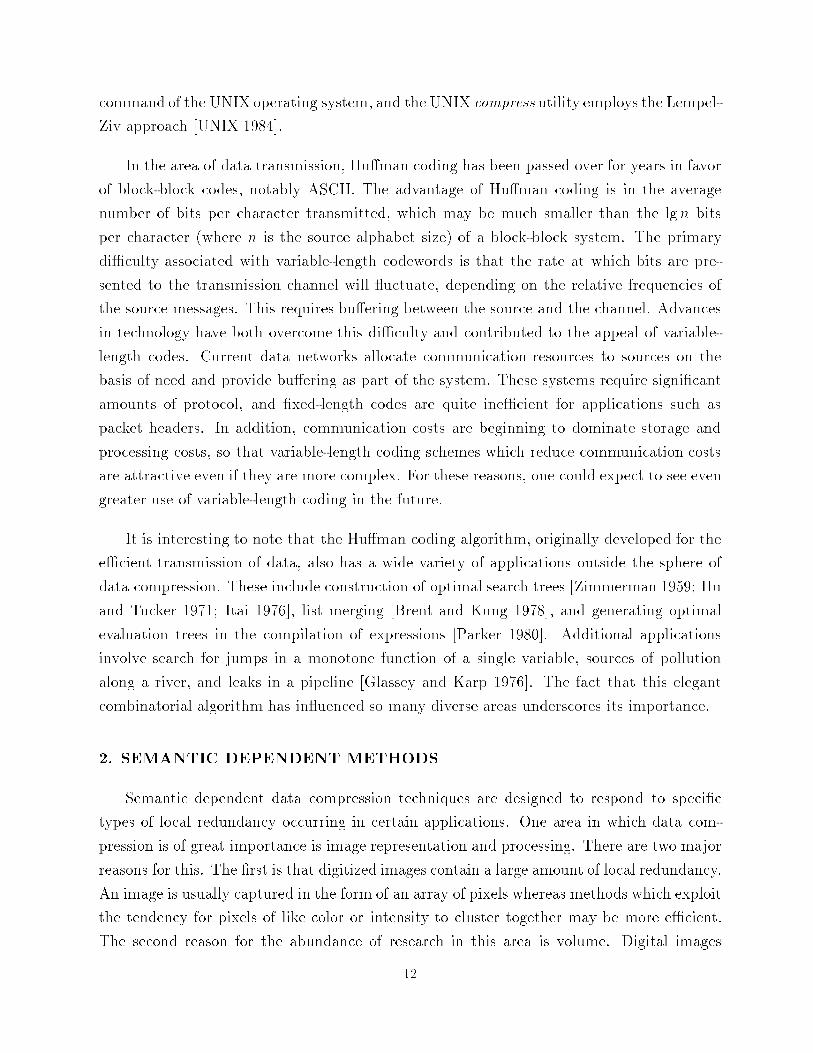
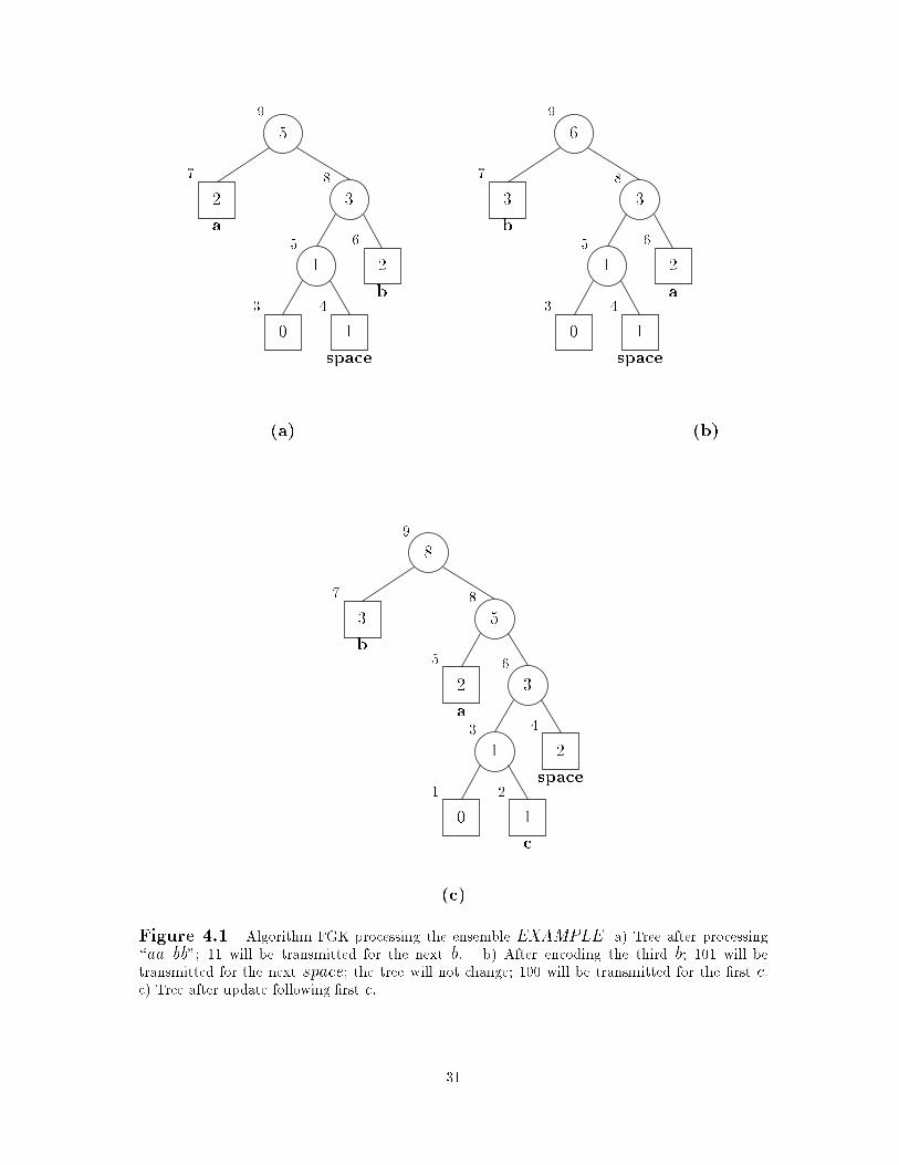
unused messages has appeared. In Figure 4.1, a simple example is given. At each node a

count of occurrences of the corresponding message is stored. Nodes are numbered indicating

their position in the sibling property ordering. The updating of the tree can be done in a

single traversal from the a

t+1

node to the root. This traversal must increment the count

for the a

t+1

node and for each of its ancestors. Nodes may be exchanged to maintain the

sibling property, but all of these exchanges involve a node on the path from a

t+1

to the root.

Figure 4.2 shows the �nal code tree formed by this process on the ensemble EXAMPLE.

Disregarding overhead, the number of bits transmitted by algorithm FGK for the EX-

AMPLE is 129. The static Hu�man algorithm would transmit 117 bits in processing the

same data. The overhead associated with the adaptive method is actually less than that of

the static algorithm. In the adaptive case the only overhead is the n lg n bits needed to rep-

resent each of the n di�erent source messages when they appear for the �rst time. (This is in

30

0 1

2

2

1

3

5

9

7

8

6

5

43

a

b

space

(a)

0 1

2

3

1

3

6

9

7

8

6

5

43

b

a

space

(b)

1

3

3

2

5

8

0 1

2

9

7

8

6

5

4

3

21

b

a

space

c

(c)

Figure 4.1 Algorithm FGK processing the ensemble EXAMPLE a) Tree after processing

\aa bb"; 11 will be transmitted for the next b. b) After encoding the third b; 101 will be

transmitted for the next space; the tree will not change; 100 will be transmitted for the �rst c.

c) Tree after update following �rst c.

31

0 2

2 3

5 5 6 754

98 10 13

17 23

40

1 2

3

4

5 6

7

8 9 10

11

12 13 14

15 16

17

a

b

c d e f

g

space

Figure 4.2 Tree formed by algorithm FGK for ensemble EXAMPLE.

fact conservative; rather than transmitting a unique code for each of the n source messages,

the sender could transmit the message's position in the list of remaining messages and save a

few bits in the average case.) In the static case, the source messages need to be sent as does

the shape of the code tree. As discussed in Section 3.2, an e�cient representation of the tree

shape requires 2n bits. Algorithm FGK compares well with static Hu�man coding on this

ensemble when overhead is taken into account. Figure 4.3 illustrates an example on which

algorithm FGK performs better than static Hu�man coding even without taking overhead

into account. Algorithm FGK transmits 47 bits for this ensemble while the static Hu�man

code requires 53.

Vitter has proved that the total number of bits transmitted by algorithm FGK for a

message ensemble of length t containing n distinct messages is bounded below by S � n+1,

where S is the performance of the static method, and bounded above by 2S+t�4n+2 [Vitter

1987]. So the performance of algorithm FGK is never much worse than twice optimal. Knuth

provides a complete implementation of algorithm FGK and a proof that the time required for

32

8

5

3

2

1

0 1

1

21

13

8

5

3

2

1

15

14

13

12

11

10

9

8

7

6

5

4

3

21

a

e

space

d

b

f

c

Figure 4.3 Tree formed by algorithm FGK for ensemble \e eae de eabe eae dcf".

each encoding or decoding operation is O(l), where l is the current length of the codeword

[Knuth 1985]. It should be noted that since the mapping is de�ned dynamically, during

transmission, the encoding and decoding algorithms stand alone; there is no additional

algorithm to determine the mapping as in static methods.

4.2 Algorithm V

The adaptive Hu�man algorithm of Vitter (algorithm V) incorporates two improvements

over algorithm FGK. First, the number of interchanges in which a node is moved upward in

the tree during a recomputation is limited to one. This number is bounded in algorithm FGK

only by l=2 where l is the length of the codeword for a

t+1

when the recomputation begins.

Second, Vitter's method minimizes the values of

P

l

i

and maxfl

i

g subject to the requirement

of minimizing

P

w

i

l

i

. The intuitive explanation of algorithm V's advantage over algorithm

FGK is as follows: as in algorithm FGK, the code tree constructed by algorithm V is the

Hu�man code tree for the pre�x of the ensemble seen so far. The adaptive methods do not

assume that the relative frequencies of a pre�x represent accurately the symbol probabilities

over the entire message. Therefore, the fact that algorithm V guarantees a tree of minimum

height (height = maxfl

i

g) and minimum external path length (

P

l

i

) implies that it is better

33

1 1 1 2

1 1

0 1

1

3

1

22

432

5 7

12

1 2

3

4

5 6

7 8

9 10

11 12

13 14

15

16

17 18

19

a s n t

e

r m

p

q

Figure 4.4 FGK tree with non-level order numbering.

suited for coding the next message of the ensemble, given that any of the leaves of the tree

may represent that next message.

These improvements are accomplished through the use of a new system for numbering

nodes. The numbering, called an implicit numbering, corresponds to a level ordering of the

nodes (from bottom to top and left to right). Figure 4.4 illustrates that the numbering

of algorithm FGK is not always a level ordering. The following invariant is maintained

in Vitter's algorithm: For each weight w, all leaves of weight w precede (in the implicit

numbering) all internal nodes of weight w. Vitter proves that this invariant enforces the

desired bound on node promotions [Vitter 1987]. The invariant also implements bottom

merging, as discussed in Section 3.2, to minimize

P

l

i

and maxfl

i

g. The di�erence between

Vitter's method and algorithm FGK is in the way the tree is updated between transmissions.

In order to understand the revised update operation, the following de�nition of a block of

nodes is necessary: Blocks are equivalence classes of nodes de�ned by u � v i� weight(u) =

weight(v) and u and v are either both leaves or both internal nodes. The leader of a block is

the highest-numbered (in the implicit numbering) node in the block. Blocks are ordered by

increasing weight with the convention that a leaf block always precedes an internal block of

the same weight. When an exchange of nodes is required to maintain the sibling property,

algorithm V requires that the node being promoted be moved to the position currently

34

occupied by the highest-numbered node in the target block.

In Figure 4.5, the Vitter tree corresponding to Figure 4.1c is shown. This is the �rst

point in EXAMPLE at which algorithm FGK and algorithm V di�er signi�cantly. At this

point, the Vitter tree has height 3 and external path length 12 while the FGK tree has

height 4 and external path length 14. Algorithm V transmits codeword 001 for the second c;

FGK transmits 1101. This demonstrates the intuition given earlier that algorithm V is better

suited for coding the next message. The Vitter tree corresponding to Figure 4.2, representing

the �nal tree produced in processing EXAMPLE, is only di�erent from Figure 4.2 in that

the internal node of weight 5 is to the right of both leaf nodes of weight 5. Algorithm V

transmits 124 bits in processing EXAMPLE, as compared with the 129 bits of algorithm

FGK and 117 bits of static Hu�man coding. It should be noted that these �gures do not

include overhead and, as a result, disadvantage the adaptive methods.

0 1

2 2 31

3 5

8

9

87

654

3

21

a b

c

space

Figure 4.5 Algorithm V processing the ensemble \aa bbb c"

Figure 4.6 ilustrates the tree built by Vitter's method for the ensemble of Figure 4.3.

Both

P

l

i

and maxfl

i

g are smaller in the tree of Figure 4.6. The number of bits transmitted

during the processing of the sequence is 47, the same used by algorithm FGK. However, if

the transmission continues with d; b; c; f or an unused letter, the cost of algorithm V will be

less than that of algorithm FGK. This again illustrates the bene�t of minimizing the external

path length (

P

l

i

) and the height (maxfl

i

g).

35

5 8

2 3

0 1 1 1

21

8 13

3 5

1 2

1 2 3 4

5

6

7

8

9

10

11

12

13 14

15

f

d

space

c b

a

e

Figure 4.6 Tree formed by algorithm V for the ensemble of Fig. 4.3.

It should be noted again that the strategy of minimizing external path length and height

is optimal under the assumption that any source letter is equally likely to occur next. Other

reasonable strategies include one which assumes locality. To take advantage of locality,

the ordering of tree nodes with equal weights could be determined on the basis of recency.

Another reasonable assumption about adaptive coding is that the weights in the current

tree correspond closely to the probabilities associated with the source. This assumption

becomes more reasonable as the length of the ensemble increases. Under this assumption,

the expected cost of transmitting the next letter is

P

p

i

l

i

�

P

w

i

l

i

, so that neither algorithm

FGK nor algorithm V has any advantage.

Vitter proves that the performance of his algorithm is bounded by S�n+1 from below

and S + t� 2n+ 1 from above [Vitter 1987]. At worst then, Vitter's adaptive method may

transmit one more bit per codeword than the static Hu�man method. The improvements

made by Vitter do not change the complexity of the algorithm; algorithm V encodes and

decodes in O(l) time as does algorithm FGK.

5. OTHER ADAPTIVE METHODS

Two more adaptive data compression methods, algorithmBSTW and Lempel-Ziv coding,

are discussed in this section. Like the adaptive Hu�man coding techniques, these methods

do not require a �rst pass to analyze the characteristics of the source. Thus, they provide

coding and transmission in real time. However, these schemes diverge from the fundamental

36

Hu�man coding approach to a greater degree than the methods discussed in Section 4.

Algorithm BSTW is a de�ned-word scheme which attempts to exploit locality. Lempel-

Ziv coding is a free-parse method; that is, the words of the source alphabet are de�ned

dynamically, as the encoding is performed. Lempel-Ziv coding is the basis for the UNIX

utility compress. Algorithm BSTW is a variable-variable scheme, while Lempel-Ziv coding

is variable-block.

5.1 Lempel-Ziv Codes

Lempel-Ziv coding represents a departure from the classic view of a code as a mapping

from a �xed set of source messages (letters, symbols or words) to a �xed set of codewords. We

coin the term free-parse to characterize this type of code, in which the set of source messages

and the codewords to which they are mapped are de�ned as the algorithm executes. While all

adaptive methods create a set of codewords dynamically, de�ned-word schemes have a �xed

set of source messages, de�ned by context (eg., in text �le processing the source messages

might be single letters; in Pascal source �le processing the source messages might be tokens).

Lempel-Ziv coding de�nes the set of source messages as it parses the ensemble.

The Lempel-Ziv algorithm consists of a rule for parsing strings of symbols from a �nite

alphabet into substrings, or words, whose lengths do not exceed a prescribed integer L

1

;

and a coding scheme which maps these substrings sequentially into uniquely decipherable

codewords of �xed length L

2

[Ziv and Lempel 1977]. The strings are selected so that they

have very nearly equal probability of occurrence. As a result, frequently-occurring symbols

are grouped into longer strings while infrequent symbols appear in short strings. This strat-

egy is e�ective at exploiting redundancy due to symbol frequency, character repetition, and

high-usage patterns. Figure 5.1 shows a small Lempel-Ziv code table. Low-frequency letters

such as Z are assigned individually to �xed-length codewords (in this case, 12 bit binary

numbers represented in base ten for readability). Frequently-occurring symbols, such as

blank (represented by [) and zero, appear in long strings. E�ective compression is achieved

when a long string is replaced by a single 12-bit code.

The Lempel-Ziv method is an incremental parsing strategy in which the coding process

is interlaced with a learning process for varying source characteristics [Ziv and Lempel 1977].

In Figure 5.1, run-length encoding of zeros and blanks is being learned.

The Lempel-Ziv algorithm parses the source ensemble into a collection of segments of

gradually increasing length. At each encoding step, the longest pre�x of the remaining source

ensemble which matches an existing table entry (�) is parsed o�, along with the character

37

Symbol string Code

A 1

T 2

AN 3

TH 4

THE 5

AND 6

AD 7

[ 8

[[ 9

[[[ 10

0 11

00 12

000 13

0000 14

Z 15

### 4095

Figure 5.1 A Lempel-Ziv code table.

(c) following this pre�x in the ensemble. The new source message, �c, is added to the code

table. The new table entry is coded as (i; c) where i is the codeword for the existing table

entry and c is the appended character. For example, the ensemble 010100010 is parsed into

f0; 1; 01; 00; 010g and is coded as f(0; 0); (0; 1); (1; 1); (1; 0); (3; 0)g. The table built for the

message ensemble EXAMPLE is shown in Figure 5.2. The coded ensemble has the form:

f (0,a), (1,space), (0,b), (3,b), (0,space), (0,c), (6,c), (6,space), (0,d), (9,d), (10,space), (0,e),

(12,e), (13,e), (5,f), (0,f), (16,f), (17,f), (0,g), (19,g), (20,g), (20) g. The string table is

represented in a more e�cient manner than in Figure 5.1; the string is represented by its

pre�x codeword followed by the extension character, so that the table entries have �xed

length. The Lempel-Ziv strategy is simple, but greedy. It simply parses o� the longest

recognized string each time rather than searching for the best way to parse the ensemble.

The Lempel-Ziv method speci�es �xed-length codewords. The size of the table and the

maximumsource message length are determined by the length of the codewords. It should be

38

Message Codeword

a 1

1space 2

b 3

3b 4

space 5

c 6

6c 7

6space 8

d 9

9d 10

10space 11

e 12

12e 13

13e 14

5f 15

f 16

16f 17

17f 18

g 19

19g 20

20g 21

Figure 5.2 Lempel-Ziv table for the message ensemble EXAMPLE (code length=173).

clear from the de�nition of the algorithm that Lempel-Ziv codes tend to be quite ine�cient

during the initial portion of the message ensemble. For example, even if we assume 3-bit

codewords for characters a through g and space and 5-bit codewords for table indices, the

Lempel-Ziv algorithm transmits 173 bits for ensemble EXAMPLE. This compares poorly

with the other methods discussed in this survey. The ensemble must be su�ciently long for

the procedure to build up enough symbol frequency experience to achieve good compression

over the full ensemble.

If the codeword length is not su�ciently large, Lempel-Ziv codes may also rise slowly

to reasonable e�ciency, maintain good performance brie y, and fail to make any gains once

39

the table is full and messages can no longer be added. If the ensemble's characteristics vary

over time, the method may be \stuck with" the behavior it has learned and may be unable

to continue to adapt.

Lempel-Ziv coding is asymptotically optimal, meaning that the redundancy approaches

zero as the length of the source ensemble tends to in�nity. However, for particular �nite

sequences, the compression achieved may be far from optimal [Storer and Szymanski 1982].

When the method begins, each source symbol is coded individually. In the case of 6- or 8-bit

source symbols and 12-bit codewords, the method yields as much as 50% expansion during

initial encoding. This initial ine�ciency can be mitigated somewhat by initializing the string

table to contain all of the source characters. Implementation issues are particularly important

in Lempel-Ziv methods. A straightforward implementation takes O(n

2

) time to process a

string of n symbols; for each encoding operation, the existing table must be scanned for the

longest message occurring as a pre�x of the remaining ensemble. Rodeh et al. address the

issue of computational complexity by de�ning a linear implementation of Lempel-Ziv coding

based on su�x trees [Rodeh et al. 1981]. The Rodeh et al. scheme is asymptotically optimal,

but an input must be very long in order to allow e�cient compression, and the memory

requirements of the scheme are large, O(n) where n is the length of the source ensemble.

It should also be mentioned that the method of Rodeh et al. constructs a variable-variable

code; the pair (i; c) is coded using a representation of the integers, such as the Elias codes,

for i and for c (a letter c can always be coded as the k

th

member of the source alphabet for

some k).

The other major implementation consideration involves the way in which the string table

is stored and accessed. Welch suggests that the table be indexed by the codewords (integers

1 : : : 2

L

where L is the maximum codeword length) and that the table entries be �xed-length

codeword-extension character pairs [Welch 1984]. Hashing is proposed to assist in encoding.

Decoding becomes a recursive operation, in which the codeword yields the �nal character of

the substring and another codeword. The decoder must continue to consult the table until

the retrieved codeword is 0. Unfortunately, this strategy peels o� extension characters in

reverse order and some type of stack operation must be used to reorder the source.

Storer and Szymanski present a general model for data compression which encompasses

Lempel-Ziv coding [Storer and Szymanski 1982]. Their broad theoretical work compares

classes of macro schemes, where macro schemes include all methods which factor out du-

plicate occurrences of data and replace them by references either to the source ensemble or

to a code table. They also contribute a linear-time Lempel-Ziv-like algorithm with better

40

performance than the standard Lempel-Ziv method.

Rissanen extends the Lempel-Ziv incremental parsing approach [Rissanen 1983]. Aban-

doning the requirement that the substrings partition the ensemble, the Rissanen method

gathers \contexts" in which each symbol of the string occurs. The contexts are substrings

of the previously encoded string (as in Lempel-Ziv), have varying size, and are in general

overlapping. The Rissanen method hinges upon the identi�cation of a design parameter

capturing the concept of \relevant" contexts. The problem of �nding the best parameter is

undecidable, and Rissanen suggests estimating the parameter experimentally.

As mentioned earlier, Lempel-Ziv coding is the basis for the UNIX utility compress and

is one of the methods commonly used in �le archival programs. The archival system PKARC

uses Welch's implementation, as does compress. The compression provided by compress is

generally much better than that achieved by compact (the UNIX utility based on algorithm

FGK), and takes less time to compute [UNIX 1984]. Typical compression values attained

by compress are in the range of 50{60%.

5.2 Algorithm BSTW

The most recent of the algorithms surveyed here is due to Bentley, Sleator, Tarjan

and Wei [Bentley et al. 1986]. This method, algorithm BSTW, possesses the advantage

that it requires only one pass over the data to be transmitted yet has performance which

compares well to that of the static two-pass method along the dimension of number of bits

per word transmitted. This number of bits is never much larger than the number of bits

transmitted by static Hu�man coding (in fact, is usually quite close), and can be signi�cantly

better. Algorithm BSTW incorporates the additional bene�t of taking advantage of locality

of reference, the tendency for words to occur frequently for short periods of time then fall

into long periods of disuse. The algorithm uses a self-organizing list as an auxiliary data

structure and employs shorter encodings for words near the front of this list. There are many

strategies for maintaining self-organizing lists (see [Hester and Hirschberg 1985]); algorithm

BSTW uses move-to-front.

A simple example serves to outline the method of algorithm BSTW. As in other adaptive

schemes, sender and receiver maintain identical representations of the code; in this case

message lists which are updated at each transmission, using the move-to-front heuristic.

These lists are initially empty. When message a

t

is transmitted, if a

t

is on the sender's list,

he transmits its current position. He then updates his list by moving a

t

to position 1 and

shifting each of the other messages down one position. The receiver similarly alters his word

41

list. If a

t

is being transmitted for the �rst time, then k+1 is the \position" transmitted, where

k is the number of distinct messages transmitted so far. Some representation of the message

itself must be transmitted as well, but just this �rst time. Again, a

t

is moved to position one

by both sender and receiver subsequent to its transmission. For the ensemble \abcadeabfd",

the transmission would be (for ease of presentation, list positions are represented in base

ten): 1 a 2 b 3 c 3 4 d 5 e 3 5 6 f 5.

As the example shows, algorithm BSTW transmits each source message once; the rest

of its transmission consists of encodings of list positions. Therefore, an essential feature of

algorithm BSTW is a reasonable scheme for representation of the integers. The methods

discussed by Bentley et al. are the Elias codes presented in Section 3.3. The simple scheme,

code , involves pre�xing the binary representation of the integer i with blg ic zeros. This

yields a pre�x code with the length of the codeword for i equal to 2blg ic + 1. Greater

compression can be gained through use of the more sophisticated scheme, �, which encodes

an integer i in 1 + blg ic+ 2b(lg(1 + blg ic)c bits.

A message ensemble on which algorithm BSTW is particularly e�cient, described by

Bentley et al., is formed by repeating each of n messages n times, for example 1

n

2

n

3

n

: : : n

n

.

Disregarding overhead, a static Hu�man code uses n

2

lg n bits (or lg n bits per message),

while algorithm BSTW uses n

2

+ 2

P

n

i=1

blg ic (which is less than or equal to n

2

+ 2n lg n,

or O(1) bits per message). The overhead for algorithm BSTW consists of just the n lg n bits

needed to transmit each source letter once. As discussed in Section 3.2, the overhead for static

Hu�man coding includes an additional 2n bits. The locality present in ensemble EXAMPLE

is similar to that in the above example. The transmission e�ected by algorithm BSTW is:

1 a 1 2 space 3 b 1 1 2 4 c 1 1 1 2 5 d 1 1 1 1 2 6 e 1 1 1 1 1 2 7 f 1 1 1 1 1 1 1 8 g 1 1 1 1 1 1 1.

Using 3 bits for each source letter (a through g and space) and the Elias code � for list

positions, the number of bits used is 81, which is a great improvement over all of the other

methods discussed (only 69% of the length used by static Hu�man coding). This could be

improved further by the use of Fibonacci codes for list positions.

In [Bentley et al. 1986] a proof is given that with the simple scheme for encoding integers,

the performance of algorithm BSTW is bounded above by 2S +1, where S is the cost of the

static Hu�man coding scheme. Using the more sophisticated integer encoding scheme, the

bound is 1+S+2 lg(1+S). A key idea in the proofs given by Bentley et al. is the fact that,

using the move-to-front heuristic, the integer transmitted for a message a

t

will be one more

than the number of di�erent words transmitted since the last occurrence of a

t

. Bentley et

al. also prove that algorithm BSTW is asymptotically optimal.

42

An implementation of algorithm BSTW is described in great detail in [Bentley et al.

1986]. In this implementation, encoding an integer consists of a table lookup; the codewords

for the integers from 1 to n+1 are stored in an array indexed from 1 to n+1. A binary trie is

used to store the inverse mapping, from codewords to integers. Decoding an Elias codeword

to �nd the corresponding integer involves following a path in the trie. Two interlinked data

structures, a binary trie and a binary tree, are used to maintain the word list. The trie

is based on the binary encodings of the source words. Mapping a source message a

i

to its

list position p involves following a path in the trie, following a link to the tree, and then

computing the symmetric order position of the tree node. Finding the source message a

i

in

position p is accomplished by �nding the symmetric order position p in the tree and returning

the word stored there. Using this implementation, the work done by sender and receiver is

O(length(a

i

) + length(w)) where a

i

is the message being transmitted and w the codeword

representing a

i

's position in the list. If the source alphabet consists of single characters, then

the complexity of algorithm BSTW is just O(length(w)).

The move-to-front scheme of Bentley et al. was independently developed by Elias in his

paper on interval encoding and recency rank encoding [Elias 1987]. Recency rank encoding

is equivalent to algorithm BSTW. The name emphasizes the fact, mentioned above, that

the codeword for a source message represents the number of distinct messages which have

occurred since its most recent occurrence. Interval encoding represents a source message by

the total number of messages which have occurred since its last occurrence (equivalently,

the length of the interval since the last previous occurrence of the current message). It is

obvious that the length of the interval since the last occurrence of a message a

t

is at least

as great as its recency rank, so that recency rank encoding never uses more, and generally

uses fewer, symbols per message than interval encoding. The advantage to interval encoding

is that it has a very simple implementation and can encode and decode selections from a

very large alphabet (a million letters, for example) at a microsecond rate [Elias 1987]. The

use of interval encoding might be justi�ed in a data transmission setting, where speed is the

essential factor.

Ryabko also comments that the work of Bentley et al. coincides with many of the results

in a paper in which he considers data compression by means of a \book stack" (the books

represent the source messages and as a \book" occurs it is taken from the stack and placed

on top) [Ryabko 1987]. Horspool and Cormack have considered move-to-front, as well as

several other list organization heuristics, in connection with data compression [Horspool and

Cormack 1987].

43

6. EMPIRICAL RESULTS

Empirical tests of the e�ciencies of the algorithms presented here are reported in [Bentley

et al. 1986; Knuth 1985; Schwartz and Kallick 1964; Vitter 1987; Welch 1984]. These exper-

iments compare the number of bits per word required and processing time is not reported.

While theoretical considerations bound the performance of the various algorithms, experi-

mental data is invaluable in providing additional insight. It is clear that the performance of

each of these methods is dependent upon the characteristics of the source ensemble.

Schwartz and Kallick test an implementation of static Hu�man coding in which bot-

tom merging is used to determine codeword lengths and all codewords of a given length are

sequential binary numbers [Schwartz and Kallick 1964]. The source alphabet in the experi-

ment consists of 5,114 frequently-used English words, 27 geographical names, 10 numerals,

14 symbols, and 43 su�xes. The entropy of the document is 8.884 binary digits per message

and the average codeword constructed has length 8.920. The same document is also coded

one character at a time. In this case, the entropy of the source is 4.03 and the coded ensemble

contains an average of 4.09 bits per letter. The redundancy is low in both cases. However,

the relative redundancy (i.e., redundancy/entropy) is lower when the document is encoded

by words.

Knuth describes algorithm FGK's performance on three types of data: a �le containing

the text of Grimm's �rst ten Fairy Tales, text of a technical book, and a �le of graphical

data [Knuth 1985]. For the �rst two �les, the source messages are individual characters

and the alphabet size is 128. The same data is coded using pairs of characters, so that

the alphabet size is 1968. For the graphical data, the number of source messages is 343.

In the case of the Fairy Tales the performance of FGK is very close to optimum, although

performance degrades with increasing �le size. Performance on the technical book is not

as good, but is still respectable. The graphical data proves harder yet to compress, but

again FGK performs reasonably well. In the latter two cases, the trend of performance

degradation with �le size continues. De�ning source messages to consist of character pairs

results in slightly better compression, but the di�erence would not appear to justify the

increased memory requirement imposed by the larger alphabet.

Vitter tests the performance of algorithms V and FGK against that of static Hu�man

coding. Each method is run on data which includes Pascal source code, the T

E

X source

of the author's thesis, and electronic mail �les [Vitter 1987]. Figure 6.1 summarizes the

results of the experiment for a small �le of text. The performance of each algorithm is

44

n k Static Alg. V Alg. FGK

100 96 83.0 71.1 82.4

500 96 83.0 80.8 83.5

961 97 83.5 82.3 83.7

Figure 6.1 Simulation results for a small text �le [Vitter 1987]; n = �le size in 8-bit bytes, k

= number of distinct messages.

measured by the number of bits in the coded ensemble and overhead costs are not included.

Compression achieved by each algorithm is represented by the size of the �le it creates, given

as a percentage of the original �le size. Figure 6.2 presents data for Pascal source code. For

the T

E

X source, the alphabet consists of 128 individual characters; for the other two �le

types, no more than 97 characters appear. For each experiment, when the overhead costs

are taken into account, algorithm V outperforms static Hu�man coding as long as the size of

the message ensemble (number of characters) is no more than 10

4

. Algorithm FGK displays

slightly higher costs, but never more than 100:4% of the static algorithm.

n k Static Alg. V Alg. FGK

100 32 57.4 56.2 58.9

500 49 61.5 62.2 63.0

1000 57 61.3 61.8 62.4

10000 73 59.8 59.9 60.0

12067 78 59.6 59.8 59.9

Figure 6.2 Simulation results for Pascal source code [Vitter 1987]; n = �le size in bytes, k =

number of distinct messages.

Witten et al. compare adaptive arithmetic coding with adaptive Hu�man coding [Wit-

ten et al. 1987]. The version of arithmetic coding tested employs single-character adaptive

frequencies and is a mildly optimized C implementation. Witten et al. compare the results

provided by this version of arithmetic coding with the results achieved by the UNIX com-

pact program (compact is based on algorithm FGK). On three large �les which typify data

compression applications, compression achieved by arithmetic coding is better than that

45

provided by compact, but only slightly better (average �le size is 98% of the compacted size).

A �le over a three-character alphabet, with very skewed symbol probabilities, is encoded by

arithmetic coding in less than one bit per character; the resulting �le size is 74% of the size

of the �le generated by compact. Witten et al. also report encoding and decoding times.

The encoding time of arithmetic coding is generally half of the time required by the adaptive

Hu�man coding method. Decode time averages 65% of the time required by compact. Only

in the case of the skewed �le are the time statistics quite di�erent. Arithmetic coding again

achieves faster encoding, 67% of the time required by compact. However, compact decodes

more quickly, using only 78% of the time of the arithmetic method.

Bentley et al. use C and Pascal source �les, TROFF source �les, and a terminal session

transcript of several hours for experiments which compare the performance of algorithm

BSTW to static Hu�man coding. Here the de�ned words consist of two disjoint classes,

sequences of alphanumeric characters and sequences of nonalphanumeric characters. The

performance of algorithm BSTW is very close to that of static Hu�man coding in all cases.

The experiments reported by Bentley et al. are of particular interest in that they incorporate

another dimension, the possibility that in the move-to-front scheme one might want to limit

the size of the data structure containing the codes to include only the m most recent words,

for some m [Bentley et al. 1986]. The tests consider cache sizes of 8, 16, 32, 64, 128 and

256. Although performance tends to increase with cache size, the increase is erratic, with

some documents exhibiting nonmonotonicity (performance which increases with cache size

to a point and then decreases when cache size is further increased).

Welch reports simulation results for Lempel-Ziv codes in terms of compression ratios

[Welch 1984]. His de�nition of compression ratio is the one given in Section 1.3, C = (average

message length)/(average codeword length). The ratios reported are: 1.8 for English text, 2

to 6 for Cobol data �les, 1.0 for oating point arrays, 2.1 for formatted scienti�c data, 2.6 for

system log data, 2.3 for source code, and 1.5 for object code. The tests involving English text

�les showed that long individual documents did not compress better than groups of short

documents. This observation is somewhat surprising, in that it seems to refute the intuition

that redundancy is due at least in part to correlation in content. For purposes of comparison,

Welch cites results of Pechura and Rubin. Pechura achieved a 1.5 compression ratio using

static Hu�man coding on �les of English text [Pechura 1982]. Rubin reports a 2.4 ratio for

English text when employing a complex technique for choosing the source messages to which

Hu�man coding is applied [Rubin 1976]. These results provide only a very weak basis for

comparison, since the characteristics of the �les used by the three authors are unknown. It

is very likely that a single algorithm may produce compression ratios ranging from 1.5 to

46

2.4, depending upon the source to which it is applied.

7. SUSCEPTIBILITY TO ERROR

The discrete noiseless channel is, unfortunately, not a very realistic model of a commu-

nication system. Actual data transmission systems are prone to two types of error: phase

error, in which a code symbol is lost or gained; and amplitude error, in which a code symbol

is corrupted [Neumann 1962]. The degree to which channel errors degrade transmission is

an important parameter in the choice of a data compression method. The susceptibility to

error of a coding algorithm depends heavily on whether the method is static or adaptive.

7.1 Static Codes

It is generally known that Hu�man codes tend to be self-correcting [Standish 1980]. That

is, a transmission error tends not to propagate too far. The codeword in which the error

occurs is incorrectly received and it is likely that several subsequent codewords are misin-

terpreted but, before too long, the receiver is back in synchronization with the sender. In a

static code, synchronization means simply that both sender and receiver identify the begin-

nings of the codewords in the same way. In Figure 7.1, an example is used to illustrate the

ability of a Hu�man code to recover from phase errors. The message ensemble \BCDAEB"

is encoded using the Hu�man code of Figure 3.4 where the source letters a

1

: : : a

5

represent

A : : :E respectively, yielding the coded ensemble \0110100011000011". Figure 7.1 demon-

strates the impact of loss of the �rst bit, the second bit, or the fourth bit. The dots show

the way in which each line is parsed into codewords. The loss of the �rst bit results in

re-synchronization after the third bit so that only the �rst source message (B) is lost (re-

placed by AA). When the second bit is lost, the �rst eight bits of the coded ensemble are

misinterpreted and synchronization is regained by bit 9. Dropping the fourth bit causes the

same degree of disturbance as dropping the second.

0 1 1 . 0 1 0 . 0 0 1 . 1 . 0 0 0 . 0 1 1 . coded ensemble BCDAEB

1 . 1 . 0 1 0 . 0 0 1 . 1 . 0 0 0 . 0 1 1 . bit 1 is lost, interpreted as AACDAEB

0 1 0 . 1 . 0 0 0 . 1 . 1 . 0 0 0 . 0 1 1 . bit 2 is lost, interpreted as CAEAAEB

0 1 1 . 1 . 0 0 0 . 1 . 1 . 0 0 0 . 0 1 1 . bit 4 is lost, interpreted as BAEAAEB

Figure 7.1 Recovery from phase errors

The e�ect of amplitude errors is demonstrated in Figure 7.2. The format of the illustra-

47

tion is the same as that in Figure 7.1. This time bits 1, 2, and 4 are inverted rather than

lost. Again synchronization is regained almost immediately. When bit 1 or bit 2 is changed,

only the �rst three bits (the �rst character of the ensemble) are disturbed. Inversion of bit

four causes loss of synchronization through the ninth bit. A very simple explanation of the

self-synchronization present in these example can be given. Since many of the codewords

end in the same sequence of digits, the decoder is likely to reach a leaf of the Hu�man code

tree at one of the codeword boundaries of the original coded ensemble. When this happens,

the decoder is back in synchronization with the encoder.

0 1 1 . 0 1 0 . 0 0 1 . 1 . 0 0 0 . 0 1 1 coded ensemble (BCDAEB)

1 . 1 . 1 . 0 1 0 . 0 0 1 . 1 . 0 0 0 . 0 1 1 bit 1 is inverted,

interpreted as DCDAEB

0 0 1 . 0 1 0 . 0 0 1 . 1 . 0 0 0 . 0 1 1 bit 2 is inverted,

interpreted as AAACDAEB

0 1 1 . 1 . 1 . 0 0 0 . 1 . 1 . 0 0 0 . 0 1 1 bit 4 is inverted,

interpreted as BAAEAAEB

Figure 7.2 Recovery from amplitude errors

So that self-synchronization may be discussed more carefully, the following de�nitions

are presented. (It should be noted that these de�nitions hold for arbitrary pre�x codes, so

that the discussion includes all of the codes described in Section 3.) If s is a su�x of some

codeword and there exist sequences of codewords � and � such that s� = �, then � is said to

be a synchronizing sequence for s. For example, in the Hu�man code used above, 1 is a syn-

chronizing sequence for the su�x 01 while both 000001 and 011 are synchronizing sequences

for the su�x 10. If every su�x (of every codeword) has a synchronizing sequence, then the

code is completely self-synchronizing. If some or none of the proper su�xes have synchroniz-

ing sequences, then the code is, respectively, partially- or never-self-synchronizing. Finally, if

there exists a sequence � which is a synchronizing sequence for every su�x, � is de�ned to be

a universal synchronizing sequence. The code used in the examples above is completely self-

synchronizing, and has universal synchronizing sequence 00000011000. Gilbert and Moore

prove that the existence of a universal synchronizing sequence is a necessary as well as a

su�cient condition for a code to be completely self-synchronizing [Gilbert and Moore 1959].

They also state that any pre�x code which is completely self-synchronizing will synchronize

itself with probability 1 if the source ensemble consists of successive messages independently

chosen with any given set of probabilities. This is true since the probability of occurrence of

48

the universal synchronizing sequence at any given time is positive.

It is important to realize that the fact that a completely self-synchronizing code will re-

synchronize with probability 1 does not guarantee recovery from error with bounded delay. In

fact, for every completely self-synchronizing pre�x code with more than two codewords, there

are errors within one codeword which cause unbounded error propagation [Neumann 1962].

In addition, pre�x codes are not always completely self-synchronizing. Bobrow and Hakimi

state a necessary condition for a pre�x code with codeword lengths l

1

: : : l

r

to be completely

self-synchronizing: the greatest common divisor of the l

i

must be equal to one [Bobrow

and Hakimi 1969]. The Hu�man code f00; 01; 10; 1100; 1101; 1110; 1111g is not completely

self-synchronizing, but is partially self-synchronizing since su�xes 00, 01 and 10 are synchro-

nized by any codeword. The Hu�man code f000; 0010; 0011; 01; 100; 1010; 1011; 100; 111g is

never-self-synchronizing. Examples of never-self-synchronizing Hu�man codes are di�cult

to construct, and the example above is the only one with fewer than 16 source messages.

Sti�er proves that a code is never-self-synchronizing if and only if none of the proper su�xes

of the codewords are themselves codewords [Sti�er 1971].

The conclusions which may be drawn from the above discussion are: while it is common

for Hu�man codes to self-synchronize, this is not guaranteed; and when self-synchronization

is assured, there is no bound on the propagation of the error. An additional di�culty is that

self-synchronization provides no indication that an error has occurred.

The problem of error detection and correction in connection with Hu�man codes has

not received a great deal of attention. Several ideas on the subject are reported here.

Rudner states that synchronizing sequences should be as short as possible to minimize re-

synchronization delay. In addition, if a synchronizing sequence is used as the codeword for a

high probability message, then re-synchronization will be more frequent. A method for con-

structing a minimum-redundancy code having the shortest possible synchronizing sequence

is described by Rudner [Rudner 1971]. Neumann suggests purposely adding some redun-

dancy to Hu�man codes in order to permit detection of certain types of errors [Neumann

1962]. Clearly this has to be done carefully, so as not to negate the redundancy reduction

provided by Hu�man coding. McIntyre and Pechura cite data integrity as an advantage of

the codebook approach discussed in Section 3.2 [McIntyre and Pechura 1985]. When the

code is stored separately from the coded data, the code may be backed up to protect it from

perturbation. However, when the code is stored or transmitted with the data, it is suscep-

tible to errors. An error in the code representation constitutes a drastic loss and therefore

extreme measures for protecting this part of the transmission are justi�ed.

49

The Elias codes of Section 3.3 are not at all robust. Each of the codes and � can be

thought of as generating codewords which consist of a number of substrings such that each

substring encodes the length of the subsequent substring. For code we may think of each

codeword (x) as the concatenation of z, a string of n zeros, and b, a string of length n+ 1

(n = blg xc). If one of the zeros in substring z is lost, synchronization will be lost as the last

symbol of b will be pushed into the next codeword.

Since the 1 at the front of substring b delimits the end of z, if a zero in z is changed to

a 1, synchronization will be lost as symbols from b are pushed into the following codeword.

Similarly, if ones at the front of b are inverted to zeros, synchronization will be lost as the

codeword (x) consumes symbols from the following codeword. Once synchronization is lost,

it cannot normally be recovered.

In Figure 7.3, codewords (6), (4), (8) are used to illustrate the above ideas. In each

case, synchronization is lost and never recovered.

0 0 1 1 0 . 0 0 1 0 0 . 0 0 0 1 0 0 0 . coded integers 6, 4, 8

0 1 1 . 0 0 0 1 0 0 0 . 0 0 1 0 0 . 0 bit 2 is lost,

interpreted as 3, 8, 2, etc.

0 1 1 . 1 . 0 0 0 1 0 0 0 . 0 0 1 0 0 . 0 bit 2 is inverted,

interpreted as 3, 1, 8, 4, etc.

0 0 0 1 0 0 0 . 1 . 0 0 0 0 0 1 0 0 0 bit 3 is inverted,

interpreted as 8, 1, etc.

Figure 7.3 E�ects of errors in Elias Codes.

The Elias code � may be thought of as a three-part ramp where �(x) = zmb with z a

string of n zeros, m a string of length n + 1 with binary value v, and b a string of length

v � 1. For example, in �(16) = 00:101:0000, n = 2, v = 5, and the �nal substring is the

binary value of 16 with the leading 1 removed so that it has length v � 1 = 4. Again the

fact that each substring determines the length of the subsequent substring means that an

error in one of the �rst two substrings is disastrous, changing the way in which the rest of

the codeword is to be interpreted. And, like code , code � has no properties which aid in

regaining synchronization once it has been lost.

The Fibonacci codes of Section 3.3, on the other hand, are quite robust. This robustness

is due to the fact that every codeword ends in the substring 11 and that substring can appear

50

nowhere else in a codeword. If an error occurs anywhere other than in the 11 substring, the

error is contained within that one codeword. It is possible that one codeword will become

two (see the sixth line of Figure 7.4), but no other codewords will be disturbed. If the

last symbol of a codeword is lost or changed, the current codeword will be fused with its

successor, so that two codewords are lost. When the penultimate bit is disturbed, up to

three codewords can be lost. For example, the coded message 011.11.011 becomes 0011.1011

if bit 2 is inverted. The maximum disturbance resulting from either an amplitude error or a

phase error is the disturbance of three codewords.

In Figure 7.4, some illustrations based on the Fibonacci coding of ensemble EXAMPLE

as shown in Figure 3.9 are given. When bit 3 (which is not part of a 11 substring) is lost or

changed, only a single codeword is degraded. When bit 6 (the �nal bit of the �rst codeword)

is lost or changed, the �rst two codewords are incorrectly decoded. When bit 20 is changed,

the �rst b is incorrectly decoded as fg.

0 0 0 0 1 1 . 0 0 0 0 1 1 . 0 0 0 1 1 . 0 1 0 1 1 . 0 1 0 1 1 . coded ensemble \aa bb".

0 0 0 1 1 . 0 0 0 0 1 1 . 0 0 0 1 1 . 0 1 0 1 1 . 0 1 0 1 1 . bit 3 is lost,

interpreted as \ a bb".

0 0 1 0 1 1 . 0 0 0 0 1 1 . 0 0 0 1 1 . 0 1 0 1 1 . 0 1 0 1 1 . bit 3 is inverted,

interpreted as \?a bb".

0 0 0 0 1 0 0 0 0 1 1 . 0 0 0 1 1 . 0 1 0 1 1 . 0 1 0 1 1 . bit 6 is lost,

interpreted as \? bb".

0 0 0 0 1 0 0 0 0 0 1 1 . 0 0 0 1 1 . 0 1 0 1 1 . 0 1 0 1 1 . bit 6 is inverted,

interpreted as \? bb".

0 0 0 0 1 1 . 0 0 0 0 1 1 . 0 0 0 1 1 . 0 1 1 . 1 1 . 0 1 0 1 1 . bit 20 is inverted,

interpreted as \aa fgb".

Figure 7.4 E�ects of errors in Fibonacci Codes.

7.2 Adaptive Codes

Adaptive codes are far more adversely a�ected by transmission errors than are static

codes. For example, in the case of a adaptive Hu�man code, even though the receiver may

re-synchronize with the sender in terms of correctly locating the beginning of a codeword, the

information lost represents more than a few bits or a few characters of the source ensemble.

51

The fact that sender and receiver are dynamically rede�ning the code indicates that by the

time synchronization is regained, they may have radically di�erent representations of the

code. Synchronization as de�ned in Section 7.1 refers to synchronization of the bit stream,

which is not su�cient for adaptive methods. What is needed here is code synchronization,

that is, synchronization of both the bit stream and the dynamic data structure representing

the current code mapping.

There is no evidence that adaptive methods are self-synchronizing. Bentley et al. note

that, in algorithm BSTW, loss of synchronization can be catastrophic, whereas this is not

true with static Hu�man coding [Bentley et al. 1986]. Ziv and Lempel recognize that the

major drawback of their algorithm is its susceptibility to error propagation [Ziv and Lempel

1977]. Welch also considers the problem of error tolerance of Lempel-Ziv codes and suggests

that the entire ensemble be embedded in an error-detecting code [Welch 1984]. Neither static

nor adaptive arithmetic coding has the ability to tolerate errors.

8. NEW DIRECTIONS

Data compression is still very much an active research area. This section suggests pos-

sibilities for further study.

The discussion of Section 7 illustrates the susceptibility to error of the codes presented

in this survey. Strategies for increasing the reliability of these codes while incurring only a

moderate loss of e�ciency would be of great value. This area appears to be largely unex-

plored. Possible approaches include embedding the entire ensemble in an error-correcting

code or reserving one or more codewords to act as error ags. For adaptive methods it may

be necessary for receiver and sender to verify the current code mapping periodically.

For adaptive Hu�man coding, Gallager suggests an \aging" scheme, whereby recent

occurrences of a character contribute more to its frequency count than do earlier occurrences

[Gallager 1978]. This strategy introduces the notion of locality into the adaptive Hu�man

scheme. Cormack and Horspool describe an algorithm for approximating exponential aging

[Cormack and Horspool 1984]. However, the e�ectiveness of this algorithm has not been

established.

Both Knuth and Bentley et al. suggest the possibility of using the \cache" concept to

exploit locality and minimize the e�ect of anomalous source messages. Preliminary empirical

results indicate that this may be helpful [Knuth 1985; Bentley et al. 1986]. A problem

related to the use of a cache is overhead time required for deletion. Strategies for reducing

52

the cost of a deletion could be considered. Another possible extension to algorithm BSTW

is to investigate other locality heuristics. Bentley et al. prove that intermittent-move-to-

front (move-to-front after every k occurrences) is as e�ective as move-to-front [Bentley et

al. 1986]. It should be noted that there are many other self-organizing methods yet to

be considered. Horspool and Cormack describe experimental results which imply that the

transpose heuristic performs as well as move-to-front, and suggest that it is also easier to

implement [Horspool and Cormack 1987].

Several aspects of free-parse methods merit further attention. Lempel-Ziv codes appear

to be promising, although the absence of a worst-case bound on the redundancy of an

individual �nite source ensemble is a drawback. The variable-block type Lempel-Ziv codes

have been implemented with some success [ARC 1986] and the construction of a variable-

variable Lempel-Ziv code has been sketched [Ziv and Lempel 1978]. The e�ciency of the

variable-variable model should be investigated. In addition, an implementation of Lempel-

Ziv coding which combines the time e�ciency of Rodeh et al. method with more e�cient

use of space is worthy of consideration.

Another important research topic is the development of theoretical models for data

compression which address the problem of local redundancy. Models based on Markov chains

may be exploited to take advantage of interaction between groups of symbols. Entropy

tends to be overestimated when symbol interaction is not considered. Models which exploit

relationships between source messages may achieve better compression than predicted by

an entropy calculation based only upon symbol probabilities. The use of Markov modeling

is considered by Llewellyn and by Langdon and Rissanen [Llewellyn 1987; Langdon and

Rissanen 1983].

9. SUMMARY

Data compression is a topic of much importance and many applications. Methods of

data compression have been studied for almost four decades. This paper has provided an

overview of data compression methods of general utility. The algorithms have been evaluated

in terms of the amount of compression they provide, algorithm e�ciency, and susceptibility

to error. While algorithm e�ciency and susceptibility to error are relatively independent

of the characteristics of the source ensemble, the amount of compression achieved depends

upon the characteristics of the source to a great extent.

Semantic dependent data compression techniques, as discussed in Section 2, are special-

53

purpose methods designed to exploit local redundancy or context information. A semantic

dependent scheme can usually be viewed as a special case of one or more general-purpose

algorithms. It should also be noted that algorithm BSTW is a general-purpose technique

which exploits locality of reference, a type of local redundancy.

Susceptibility to error is the main drawback of each of the algorithms presented here.

Although channel errors are more devastating to adaptive algorithms than to static ones,

it is possible for an error to propagate without limit even in the static case. Methods of

limiting the e�ect of an error on the e�ectiveness of a data compression algorithm should be

investigated.

REFERENCES

Abramson, N. 1963. Information Theory and Coding. McGraw-Hill, New York.

Apostolico, A. and Fraenkel, A. S. 1985. Robust Transmission of Unbounded

Strings Using Fibonacci Representations. Tech. Rep. CS85-14, Dept. of Appl.

Math., The Weizmann Institute of Science, Rehovot, Sept.

ARC File Archive Utility. 1986. Version 5.1. System Enhancement Associates.

Wayne, N. J.

Ash, R. B. 1965. Information Theory. Interscience Publishers, New York.

Bentley, J. L., Sleator, D. D., Tarjan, R. E., and Wei, V. K. 1986. A Locally

Adaptive Data Compression Scheme. Commun. ACM 29, 4 (Apr.), 320{330.

Bobrow, L. S., and Hakimi, S. L. 1969. Graph Theoretic Pre�x Codes and

Their Synchronizing Properties. Inform. Contr. 15, 1 (July), 70{94.

Brent, R., and Kung, H. T. 1978. Fast Algorithms for Manipulating Formal

Power Series. J. ACM 25, 4 (Oct.), 581{595.

Capocelli, R. M., Giancarlo, R., and Taneja, I. J. 1986. Bounds on the Redun-

dancy of Hu�man Codes. IEEE Trans. Infor. Theory 32, 6 (Nov.), 854{857.

Cappellini, V., Ed. 1985. Data Compression and Error Control Techniques

with Applications. Academic Press, London.

Connell, J. B. 1973. A Hu�man-Shannon-Fano Code. Proc. IEEE 61, 7 (July),

1046{1047.

Cormack, G. V. 1985. Data Compression on a Database System. Commun.

ACM 28, 12 (Dec.), 1336{1342.

Cormack, G. V., and Horspool, R. N. 1984. Algorithms for Adaptive Hu�man

Codes. Inform. Process. Lett. 18, 3 (Mar.), 159{165.

Cortesi, D. 1982. An E�ective Text-Compression Algorithm.BYTE 7, 1 (Jan.),

397{403.

Cot, N. 1977. Characterization and Design of Optimal Pre�x Codes. Ph. D.

dissertation, Computer Science Dept., Stanford Univ., Stanford, Calif.

Elias, P. 1975. Universal Codeword Sets and Representations of the Integers.

IEEE Trans. Inform. Theory 21, 2 (Mar.), 194{203.

Elias, P. 1987. Interval and Recency Rank Source Coding: Two On-Line Adap-

tive Variable-Length Schemes.

IEEE Trans. Inform. Theory 33, 1 (Jan.), 3{10.

Faller, N. 1973. An Adaptive System for Data Compression. Record of the

7th Asilomar Conf. on Circuits, Systems and Computers (Paci�c Grove, Ca.,

Nov.), 593{597.

Fano, R. M. 1949. Transmission of Information. M. I. T. Press, Cambridge,

Mass.

Fraenkel, A. S. and Klein, S. T. 1985. Robust Universal Complete Codes As

Alternatives to Hu�man Codes. Tech. Report CS85-16, Dept. of Appl. Math.,

The Weizmann Institute of Science, Rehovot, Oct.

Fraenkel, A. S., Mor, M., and Perl, Y. 1983. Is Text Compression by Pre�xes

and Su�xes Practical? Acta Inf. 20, 4 (Dec.), 371{375.

Gallager, R. G. 1968. Information Theory and Reliable Communication, Wiley,

New York.

Gallager, R. G. 1978. Variations on a Theme by Hu�man. IEEE Trans. Inform.

Theory 24, 6 (Nov.), 668{674.

Garey, M. R. 1974. Optimal Binary Search Trees with Restricted Maximal

Depth. SIAM J. Comput. 3, 2 (June), 101{110.

Gilbert, E. N. 1971. Codes Based on Inaccurate Source Probabilities. IEEE

Trans. Inform. Theory 17, 3, (May), 304{314.

Gilbert, E. N., and Moore, E. F. 1959. Variable-Length Binary Encodings. Bell

System Tech. J. 38, 4 (July), 933{967.

Glassey, C. R., and Karp, R. M. 1976. On the Optimality of Hu�man Trees.

SIAM J. Appl. Math 31, 2 (Sept.), 368{378.

Gonzalez, R. C., and Wintz, P. 1977. Digital Image Processing. Addison-

Wesley, Reading, Mass.

Hahn, B. 1974. A New Technique for Compression and Storage of Data. Com-

mun. ACM 17, 8 (Aug.), 434{436.

Hester, J. H., and Hirschberg, D. S. 1985. Self-Organizing Linear Search. ACM

Comput. Surv. 17, 3 (Sept.), 295{311.

Horspool, R. N. and Cormack, G. V. 1987. A Locally Adaptive Data Com-

pression Scheme. Commun. ACM 16, 2 (Sept.), 792{794.

Hu, T. C., and Tan, K. C. 1972. Path Length of Binary Search Trees. SIAM

J. Appl. Math 22, 2 (Mar.), 225{234.

Hu, T. C., and Tucker, A. C. 1971. Optimal Computer Search Trees and

Variable-Length Alphabetic Codes. SIAM J. Appl. Math 21, 4 (Dec.), 514{

532.

Hu�man, D. A. 1952. A Method for the Construction of Minimum-

Redundancy Codes. Proc. IRE 40, 9 (Sept.), 1098{1101.

Ingels, F. M. 1971. Information and Coding Theory. Intext, Scranton, Penn.

Itai, A. 1976. Optimal Alphabetic Trees. SIAM J. Comput. 5, 1 (Mar.), 9{18.

Karp, R. M. 1961. Minimum Redundancy Coding for the Discrete Noiseless

Channel. IRE Trans. Inform. Theory 7, 1 (Jan.), 27{38.

Knuth, D. E. 1971. OptimumBinary Search Trees. Acta Inf. 1, 1 (Jan.), 14{25.

Knuth, D. E. 1985. Dynamic Hu�man Coding. J. Algorithms 6, 2 (June),

163{180.

Krause, R. M. 1962. Channels Which Transmit Letters of Unequal Duration.

Inform. Contr. 5, 1 (Mar.), 13{24.

Laeser, R. P., McLaughlin, W. I., and Wol�, D. M. 1986. Engineering Voyager

2's Encounter with Uranus Scienti�c American 255, 5 (Nov.), 36{45.

Langdon, G. G., and Rissanen, J. J. 1983. A Double-Adaptive File Compres-

sion Algorithm. IEEE Trans. Comm. 31, 11 (Nov.), 1253{1255.

Llewellyn, J. A. 1987. Data Compression for a Source with Markov Charac-

teristics. Computer J. 30, 2, 149{156.

McIntyre, D. R., and Pechura, M. A. 1985. Data Compression Using Static

Hu�man Code-Decode Tables. Commun. ACM 28, 6 (June), 612{616.

Mehlhorn, K. 1980. An E�cient Algorithm for Constructing Nearly Optimal

Pre�x Codes. IEEE Trans. Inform. Theory 26, 5 (Sept.), 513{517.

Neumann, P. G. 1962. E�cient Error-Limiting Variable-Length Codes. IRE

Trans. Inform. Theory 8, 4 (July), 292{304.

Parker, D. S. 1980. Conditions for the Optimality of the Hu�man Algorithm.

SIAM J. Comput. 9, 3 (Aug.), 470{489.

Pasco, R. 1976. Source Coding Algorithms for Fast Data Compression. Ph. D.

dissertation, Dept. of Electrical Engineering, Stanford Univ., Stanford, Calif.

Pechura, M. 1982. File Archival Techniques Using Data Compression. Com-

mun. ACM 25, 9 (Sept.), 605{609.

Perl, Y., Garey, M. R., and Even, S. 1975. E�cient Generation of Optimal

Pre�x Code: Equiprobable Words Using Unequal Cost Letters. J. ACM 22, 2

(Apr.), 202{214.

PKARC FAST! File Archival Utility. 1987. Version 3.5. PKWARE, Inc. Glen-

dale, WI.

Reghbati, H. K. 1981. An Overview of Data Compression Techniques. Com-

puter 14, 4 (Apr.), 71{75.

Rissanen, J. J. 1976. Generalized Kraft Inequality and Arithmetic Coding.

IBM J. Res. Dev. 20 (May), 198{203.

Rissanen, J. J. 1983. A Universal Data Compression System. IEEE Trans.

Inform. Theory 29, 5 (Sept.), 656{664.

Rodeh, M., Pratt, V. R., and Even, S. 1981. A Linear Algorithm for Data

Compression via String Matching. J. ACM 28, 1 (Jan.), 16{24.

Rubin, F. 1976. Experiments in Text File Compression. Commun. ACM 19,

11 (Nov.), 617{623.

Rubin, F. 1979. Arithmetic Stream Coding Using Fixed Precision Registers.

IEEE Trans. Inform. Theory 25, 6 (Nov.), 672{675.

Rudner, B. 1971. Construction of Minimum-Redundancy Codes with Optimal

Synchronizing Property. IEEE Trans. Inform. Theory 17, 4 (July), 478{487.

Ruth, S. S., and Kreutzer, P. J. 1972. Data Compression for Large Business

Files. Datamation 18, 9 (Sept.), 62{66.

Ryabko, B. Y. 1987. A Locally Adaptive Data Compression Scheme.Commun.

ACM 16, 2 (Sept.), 792.

Samet, H. 1984. The Quadtree and Related Hierarchical Data Structures.ACM

Comput. Surv. 16, 2 (June), 187{260.

Schwartz, E. S. 1964. An Optimum Encoding with Minimum Longest Code

and Total Number of Digits. Inform. Contr. 7, 1 (Mar.), 37{44.

Schwartz, E. S., and Kallick, B. 1964. Generating a Canonical Pre�x Encoding.

Commun. ACM 7, 3 (Mar.), 166{169.

Severance, D. G. 1983. A Practitioner's Guide to Data Base Compression.

Inform. Systems 8, 1, 51{62.

Shannon, C. E., and Weaver, W. 1949. The Mathematical Theory of Commu-

nication. University of Illinois Press, Urbana, Ill.

Snyderman, M., and Hunt, B. 1970. The Myriad Virtues of Text Compaction.

Datamation 16, 12 (Dec.), 36{40.

Standish, T. A. 1980. Data Structure Techniques. Addison-Wesley, Reading,

Mass.

Sti�er, J. J. 1971. Theory of Synchronous Communications. Prentice-Hall,

Englewood Cli�s, N. J.

Storer, J. A., and Szymanski, T. G. 1982. Data Compression via Textual Sub-

stitution. J. ACM 29, 4 (Oct.), 928{951.

Tanaka, H. 1987. Data Structure of Hu�man Codes and Its Application to

E�cient Encoding and Decoding. IEEE Trans. Inform. Theory 33, 1 (Jan.),

154{156.

Tropper, R. 1982. Binary-Coded Text, A Text-Compression Method. BYTE

7, 4 (Apr.), 398{413.

UNIX User's Manual. 1984. 4.2. Berkeley Software Distribution, Virtual VAX-

11 Version, University of California, Berkeley.

Varn, B. 1971. Optimal Variable Length Codes (Arbitrary Symbol Cost and

Equal Code Word Probability). Inform. Contr. 19, 4 (Nov.), 289{301.

Vitter, J. S. 1987. Design and Analysis of Dynamic Hu�man Codes. J. ACM

34, 4 (Oct.), 825{845.

Wagner, R. A. 1973. Common Phrases and Minimum-Space Text Storage.

Commun. ACM 16, 3 (Mar.), 148{152.

Welch, T. A. 1984. A Technique for High-Performance Data Compression.

Computer 17, 6 (June), 8{19.

Wilkins, L. C., and Wintz, P. A. 1971. Bibliography on Data Compression,

Picture Properties and Picture Coding. IEEE Trans. Inform. Theory 17, 2,

180{197.

Witten, I. H., Neal, R. M., and Cleary, J. G. 1987. Arithmetic Coding for Data

Compression. Commun. ACM 30, 6 (June), 520{540.

Zimmerman, S. 1959. An Optimal Search Procedure. Amer. Math. Monthly

66, (Oct.), 690{693.

Ziv, J., and Lempel, A. 1977. A Universal Algorithm for Sequential Data

Compression. IEEE Trans. Inform. Theory 23, 3 (May), 337{343.

Ziv, J., and Lempel, A. 1978. Compression of Individual Sequences via Variable-

Rate Coding. IEEE Trans. Inform. Theory 24, 5 (Sept.), 530{536.