data compression for inference tasks in wireless sensor networks

DATA COMPRESSION FOR INFERENCE TASKS IN

WIRELESS SENSOR NETWORKS

BY

MO CHEN

BS, Shandong University, China, 1998

MS, Shandong University, China, 2001

DISSERTATION

Submitted in partial fulfillment of the requirements for

the degree of Doctor of Philosophy in Electrical Engineering

in the Graduate School of

Binghamton University

State University of New York

2006

iii

Accepted in partial fulfillment of the requirements for

the degree of Doctor of Philosophy in Electrical Engineering

in the Graduate School of


State University of New York

2006

March 11, 2006

Mark L. Fowler, Department of Electrical and Computer Engineering,


Xiaohua (Edward) Li Department of Electrical and Computer Engineering,


N. Eva Wu Department of Electrical and Computer Engineering,


Harold W. Lewis III, Department of Industry Engineering and System Science,


iv

Abstract

DATA COMPRESSION FOR INFERENCE TASKS IN WIRELESS

SENSOR NETWORKS

by

Mo Chen

Chair: Mark L. Fowler

In order for wireless sensor networks to exploit signal, signal data must be collected at a

multitude of sensors and must be shared among the sensors. The vast sharing of signals among

the sensors contradicts the requirements (energy efficiency, low latency and high accuracy) of

wireless networked sensor. Although many approaches have been proposed in the past (routing,

sleep modes, low-power electronics, etc.), a new aspect is proposed here: using data compression

methods as a tool for accomplishing the optimal trade-off between rate, energy, and accuracy in a

sensor network. The ability of data compression to provide energy efficiency rests on the

favorable trade between computational energy and transmission energy recently recognized in the

literature.

Because a primary task of multi-sensor systems is to make statistical inferences based on the

data collected and shared throughout the sensor system, in the viewpoint of rate, energy, and

accuracy, it is important to design data compression methods that enable rapid and low-energy

consumption sharing while causing only minimal degradation of the quantity of these inferences.

By recognizing that MSE-based compression algorithms are not appropriate for such tasks, this

dissertation stresses the development of distortion measures that effectively capture the impact of

compression on the accuracy of the inferences. Furthermore, sensor systems generally have

v

multiple inference tasks to accomplish simultaneously, and these multiple inferences generally

have conflicting requirements on compression and finding the right way to balance these conflicts

is crucial, this dissertation develops theory and algorithms that will allow the optimal trade-off

between these conflicting goals. On the other hand, these multiple tasks may occur sequentially

(and a step in the sequence could require simultaneous inferences). A task-embedded

compression method is developed to compress and send data in a sequential manner that allows

optimal attainment of the sequential tasks.

The contributions of this dissertation include: (i) strengthening data compression as a

powerful tool for achieving optimal tradeoff among energy, latency and accuracy in sensor

networks; (ii) developing new fundamental framework for compression in sensor networks that

recognize the inferential characteristics of sensor networks; (iii) developing a significant

framework for the “compression for multiple inferences” area that addresses multiple

simultaneous and sequential inferences (no results in the literature currently address this

important issue); The results of this dissertation will provide the engineer with a systematic

means for addressing Rate-Energy-Accuracy issues across the spectrum of sensor network types –

from networks of myriad microsensors to networks of several macrosensors.

vi

To my parents and Dr. Mark. L. Fowler

vii

ACHNOWLEDGEMENTS

I wish to express my sincere gratitude to my advisor, Professor Mark L. Fowler. His

guidance and encouragement throughout my dissertation have been invaluable and

unsparing. I would also like to thank Professor Xiaohua (Edward) Li for his numerous

helpful discussion and unselfish guidance concerning my research. Additionally, I am

indebted to committee members Professor N. Eva, Wu and Professor Harold W. Lewis III

for their service on my dissertation committee and for their careful reading and

evaluation of this dissertation.

From the bottom of my heart, I would like to thank my parents for their never ending

love. Moreover, I wish to thank my wife, whose affection has always been unequivocal. I

owe an incalculable debt of gratitude to them for their unfailing support. Without any of

you, this dissertation would never been possible.

Thanks, too, are in order for my friend at Binghamton University.

viii

TABLE OF CONTENTS

COMMITTEE PAGE . . . . . . . . . . . . . . . . . . . . . . . . . . . . . . . . . . . . . . . . . . . . . . . . . . iii

ABSTRACT . . . . . . . . . . . .. . . . . . . . . . . . . . . . . . . . . . . . . . . . . . . . . . . . . . . . . . . . . . . iv

DEDICATION . . . . . . . . . . . . . . . . . . . . . . . . . . . . . . . . . . . . .. . . . . . . . . . . . . . . . . . .. vi

ACHNOWLEGEMENTS . . . . . . . . . . . . . . . . . . . . . . . . . . . . . . . . . . . . . . . . . . . . . .. vii

LIST OF TABLES . . . . . . . . . . . .. . . . . . . . . . . . . . . . . . . . . . . . . . . . . . . . . . . . . . . . . . x

LIST OF FIGURES . . . . . . . . . . . . . . . . . . . . . . . . . . . . . . . . . . . . . . . . . . . . . . . . . . . . xi

LIST OF APPENDICES . . . . . . . .. . . . . . . . . . . . . . . . . . . . . . . . . . . . . . . . . . . . . . . xv

CHAPTERS

1 Introduction . . . . . . . . . . . . . . . . . . . . . . . . . . . . . . . . . . . . . . . . . . . . . . . . . . . . 1

1.1 Wireless Sensor Networks . . . . . . . . . . . . . . . . . . . . . . . . . . . . . . . . . . . . 1

1.2 Importance of Data Compression for Energy-Efficiency in Wireless

Sensor Networks . . . . . . . . . . . . . . . . . . . . . . . . . . . . . . . . . . . . . . . . . . . . 2

1.3 Compression for Inference Tasks in Wireless Sensor Networks . . . . . . . 9

2 Overview of Compression System for Inference Tasks . . . . . . . . . . . . . . . . . 13

2.1 Estimation . . . . . . . . . . . . . . . . . . . . . . . . . . . . . . . . . . . . . . . . . . . . . . . . 14

2.2 Detection . . . . . . . . . . . . . . . . . . . . . . . . . . . . . . . . . . . . . . . . . . . . . . . . . 18

2.3 Data Compression and Decompression . . . . . . . . . . . . . . . . . . . . . . . . . 20

2.3.1 Coding . . . . . . . . . . . . . . . . . . . . . . . . . . . . . . . . . . . . . . . . . . . . . 22

2.3.2 Transform . . . . . . . . . . . . . . . . . . . . . . . . . . . . . . . . . . . . . . . . . . . 23

2.3.3 Quantization . . . . . . . . . . . . . . . . . . . . . . . . . . . . . . . . . . . . . . . . . 25

2.3.4 Bit Allocation . . . . . . . . . . . . . . . . . . . . . . . . . . . . . . . . . . . . . . . . 29

2.4 Compression for inference tasks . . . . . . . . . . . . . . . . . . . . . . . . . . . . . . . 30

3 Data Compression for Parameter Estimation and Detection . . . . . . . . . .. . . . . 35

3.1 Fisher-Information-Based Data Compression for Parameter Estimation 35

3.1.1 Overview of Previous Work . . . . . . . . . . . . . . . . . . . . . . . . . . . 35

3.1.2 Fisher Information for Compression . . . . . . . . . . . . . . . . . . . . 36

3.1.3 Compressing to Maximize Fisher Information . . . . . . . . . . . . 38

3.1.4 Example Applications . . . . . . . . . . . . . . . . . . . . . . . . . . . . . . . . 48

3.1.4.1 Compression for TDOA Estimation . . . . . . . . . . . . . . . . 50

3.1.4.2 Compression for FDOA Estimation . . . . . . . . . . . . . . . . 55

ix

3.1.4.3 Compression for DOA Estimation . . . . . . . . . . . . . . . . . 62

3.1.4.4 Compression for Signal Estimation . . . . . . . . . . . . . . . . 65

3.2 Chernoff-Distance-Based Data Compression for Detection . . . . . . . . . . 68

3.2.1 Overview of Previous Work . . . . . . . . . . . . . . . . . . . . . . . . . . . 68

3.2.2 Compressing to Maximize Chernoff Distance . . . . . . . . . . . . . 72

4 Data Compression for Simultaneous Tasks of Multiple Inference Quantities . 76

4.1 Data Compression for Simultaneous Multiple Parameter Estimation

without Detection . . . . . . . . . . . . . . . . . . . . . . . . . . . . . . . . . . . . . . . . . . 77

4.1.1 Application to Simultaneous Estimation . . . . . . . . . . . . . . . . 87

4.1.1.1 Joint TDOA and DOA Estimation . . . . . . . . . . . . . . . . . 87

4.1.1.2 Simulations for Joint TDOA and DOA Estimation . . . . . 90

4.1.1.3 Joint TDOA and FDOA Estimation . . . . . . . . . . . . . . . . 91

4.1.2 Modified Distortion Measures to Include Off-Diagonals . . . .100

4.1.3 Simulations of compression using parallel auxiliary STFT

processing . . . . . . . . . . . . . . . . . . . . . . . . . . . . . . . . . . . . . . . . 108

4.2 Data Compression for Parameter Estimation with Detection . . . . . . . . 110

5 Data Compression for Sequential Tasks of Multiple Inference Quantities . . .114

5.1 Simple Detection-Then-TDOA Problem . . . . . . . . . . . . . . . . . . . . . . . . 115

5.1.1 An Algorithm for Sequential Detect-Then-TDOA . . . . . . . . . 119

5.1.2 Simulation Scenario . . . . . . . . . . . . . . . . . . . . . . . . . . . . . . . . . 120

5.2 General Sequential data compression algorithm . . . . . . . . . . . . . . . . . . 122

6 Conclusion . . . . . . . . . . . . . . . . . . . . . . . . . . . . . . . . . . . . . . . . . . . . . . . . . . . 127

APPENDICES . . . . . . . . . . . . . . . . . . . . . . . . . . . . . . . . . . . . . . . . . . . . . . . . . . . . . . . 130

BIBLIOGRAHPY . . . . . . . . . . . . . . . . . . . . . . . . . . . . . . . . . . . . . . . . . . . . . . . . . . . . 184

x

LIST OF TABLES

Table

5.1 Sequential Example, Rough Multiple Estimate - Then- Refine Estimation . 126

5.2 Sequential Example, Detection-Then - Estimation . . . . . . . . . . . . . . . . . . . 126

B.1 Fitness of the approximation model with the true mode . . . . . . . . . . . . . . . . 141

xi

LIST OF FIGURES

Figure

1.1 Non-distributed compression improves network lifespan when using direct

transmission . . . . . . . . . . . . . . . . . . . . . . . . . . . . . . . . . . . . . . . . . . . . . . . . . . . . . . . . . . 6

1.2 Result of showing improvement using compression with a simple routing

scheme . . . . . . . . . . . . . . . . . . . . . . . . . . . . . . . . . . . . . . . . . . . . . . . . . . . . . . . . . . . . . . 7

2.1 System of Compression for inference tasks, 1x and 2x are digitized sensed

measurements at sensor S1 and S2, and 1x is the decompressed data at sensor S2 . . . .14

2.2 The elements of compression-decompression process . . . . . . . . . . . . . . . . . . . . . . . . 22

2.3 Graphical representation of scalar quantization . . . . . . . . . . . . . . . . . . . . . . . . . . . . . 26

2.4 Embedded scalar quantizers0Q ,

1Q , and 2Q , of rates R = 1, 2, and 3 bits/samples . . 28

2.5 Uniform scalar quantizer with deadzone . . . . . . . . . . . . . . . . . . . . . . . . . . . . . . . . . . . 29

2.6 Framework of the compression method . . . . . . . . . . . . . . . . . . . . . . . . . . . . . . . . . . . 33

3.1 Classical set-up for compression in a distributed sensor system . . . . . . . . . . . . . . . . . 36

3.2 Compression processing, the data vectors, and their corresponding Fisher

information . . . . . . . . . . . . . . . . . . . . . . . . . . . . . . . . . . . . . . . . . . . . . . . . . . . . . . . . . .41

3.3 The spectrum of a typical FM signal used in the simulations . . . . . . . . . . . . . . . . . . 49

3.4 TDOA accuracy vs SNR of pre-compressed sensor S1 signal for a CR of 4:1; the SNR

of the sensor S2 signal was 40 dB . . . . . . . . . . . . . . . . . . . . . . . . . . . . . . . . . . . . . . . . . 56


of the sensor S2 signal was 40 dB . . . . . . . . . . . . . . . . . . . . . . . . . . . . . . . . . . . . . 56


of the sensor S2 signal was set equal to SNR1 . . . . . . . . . . . . . . . . . . . . . . . . . . . . . . . . 57


of the sensor S2 signal was set equal to SNR1 . . . . . . . . . . . . . . . . . . . . . . . . . . . . . . . . 57

xii

3.8 Reconstruction accuracy vs SNR of pre-compressed sensor 1S signal for a

compression ratio of 4:1 . . . . . . . . . . . . . . . . . . . . . . . . . . . . . . . . . . . . . . . . . . . . . . . . 58

3.9 Reconstruction accuracy vs SNR of pre-compressed sensor 1S signal for a

compression ratio of 8:1 . . . . . . . . . . . . . . . . . . . . . . . . . . . . . . . . . . . . . . . . . . . . . . . . 58

3.10 FDOA accuracy vs SNR of pre-compressed sensor S1 signal for a CR of 4:1; the SNR


3.11 FDOA accuracy vs SNR of pre-compressed sensor S1 signal for a CR of 8:1; the SNR


3.12 DOA accuracy vs SNR1 pf pre-compressed sensor 1S signal for a CR of 4:1; the SNR

of the sensor 2S signal was equal to SNR2 . . . . . . . . . . . . . . . . . . . . . . . . . . . . . . . . . . 66

3.13 DOA accuracy vs SNR1 pf pre-compressed sensor 1S signal for a CR of 8:1; the SNR

of the sensor 2S signal was equal to SNR2 . . . . . . . . . . . . . . . . . . . . . . . . . . . . . . . . . . 66

4.1 The spectrum of a typical FM signal used in the simulations . . . . . . . . . . . . . . . . . . . 91

4.2 Trade-off between TDOA and DOA accuracies as α is varied for SNR1 = 15 dB & SNR2 = 15 dB and compression ratio (a) 3.5:1 and (b) 6:1 . . . . . . . . . . . . . . . . . . . . . 92

4.3 Effect of compression ratio on (a) TDOA and (b) DOA performance . . . . . . . . . . . . 93

4.4 Trade-off between TDOA and FDOA accuracies as α is varied for compression ratio

3:1 and SNR1 = 15 dB & SNR2 = 15 dB . . . . . . . . . . . . . . . . . . . . . . . . . . . . . . . . . . . . 98

4.5 Effect of compression ratio on (a) TDOA and (b) FDOA performance. A comparison

is also made to the case of simply sending less data (“Length Reduced”) rather than

compressing the data . . . . . . . . . . . . . . . . . . . . . . . . . . . . . . . . . . . . . . . . . . . . . . . . . . 99

4.6 Comparison between the determinant optimization method (‘Area’) and weighted trace

method (‘Premeter’) and MSE for compression ratio 3:1 and SNR1 = 15 dB & SNR2 =

15 dB . . . . . . . . . . . . . . . . . . . . . . . . . . . . . . . . . . . . . . . . . . . . . . . . . . . . . . . . . . . . . 100

4.7 Geometry Adaptive TDOA/FDOA System Scheme . . . . . . . . . . . . . . . . . . . . . . . . . 104

4.8 Effect of compression ratio on CEP . . . . . . . . . . . . . . . . . . . . . . . . . . . . . . . . . . . . . . 105

4.9 Our compression framework using parallel auxiliary STFT processing to evaluate the

FIM elements . . . . . . . . . . . . . . . . . . . . . . . . . . . . . . . . . . . . . . . . . . . . . . . . . . . . . . . 109

4.10 (a) Geometry among the two pair of sensors and emitter; (b) The comparison of

difference compression algorithms on the trace of error covariance of emitter

location . . . . . . . . . . . . . . . . . . . . . . . . . . . . . . . . . . . . . . . . . . . . . . . . . . . . . . . . . . . .111

xiii

4.11 (a) Geometry among the two pair of sensors and emitter; (b) The comparison of

difference compression algorithms on the trace of error covariance of emitter

location . . . . . . . . . . . . . . . . . . . . . . . . . . . . . . . . . . . . . . . . . . . . . . . . . . . . . . . . . . . .112

5.1 Sequential Tasks with the Initial Trade-Off . . . . . . . . . . . . . . . . . . . . . . . . . . . . . . . 117

5.2 Sequential Tasks with a New Trade-Off . . . . . . . . . . . . . . . . . . . . . . . . . . . . . . . . . . 118

5.3 Trade-off for fixed task resources . . . . . . . . . . . . . . . . . . . . . . . . . . . . . . . . . . . . . . . 120

5.4 Conceptual illustration of the trade-off accomplished via choice of the β parameter. where SNR1=SNR2=15 dB . . . . . . . . . . . . . . . . . . . . . . . . . . . . . . . . . . . . . . . . . . . . . .122

5.5 Simulation results illustrating the achieved trade-offs . . . . . . . . . . . . . . . . . . . . . . . . 122

B.1 Comparison of characteristic function between true model and approximation

model . . . . . . . . . . . . . . . . . . . . . . . . . . . . . . . . . . . . . . . . . . . . . . . . . . . . . . . . . . . . . 139

B.2 Comparison of value ),),((Ι σθξ nnt ∆ and ),(Ι σ∆a under different values

of )(θξn and 2

n∆ when (a) PSNR =10 dB, (b) PSNR=15 dB . . . . . . . . . . . . . . . . . . . 142

C.1 Three-level wavelet decomposition . . . . . . . . . . . . . . . . . . . . . . . . . . . . . . . . . . . . . 148

C.2 The input and reference images . . . . . . . . . . . . . . . . . . . . . . . . . . . . . . . . . . . . . . . . 157

C.3 Reconstructed image from (a) the standard JPEG or EZW compression, (b) the

modified JPEG compression with the weight matrix 22 ji + and all-ones mask,

(c) the modified JPEG compression with the zigzag weight matrix and the example

mask, and (d) the modified EZW compression . . . . . .. . . . . . . . . . . . . . . . . . . . . . 157

C.4 Normalized correlation outputs of the reference and the input image processed

(a) without compression, (b) with JPEG or EZW compression, (c) with the

modified JPEG, and (d) with the modified EZW compression . . . . . . . . . . . . . . . 157

C.5 Compression ratio versus quality factor . . . . . . . . . . . . . . . . . . . . . . . . . . . . . . . . . 158

C.6 Reconstructed image and correlation output when q=12 . . . . . . . . . . . . . . . . . . . . 159

C.7 Reconstructed image and correlation output when q=35 . . . . . . . . . . . . . . . . . . . . 159

C.8 (a) the noisy input image; (b) normalized correlation outputs of the reference

and (a) with the modified JPEG; (c) normalized correlation outputs of the

reference and (a) with the modified EZW . . . . . . . . . . . . . . . . . . . . . . . . . . . . . . . .160

E.1 Quality of numerical evaluation of FIM via complex filter bank . . . . . . . . . . . . . . 165

E.2 Quality of numerical evaluation of FIM via STFT . . . . . . . . . . . . . . . . . . . . . . . . . 166

F.1 Example of a four-channel, full-tree cascaded analysis filter bank . . . . . . . . . . . . . 168

xiv

F.2 Example of a four-channel, full-tree cascaded synthesis filter bank . . . . . . . . . . . . . . 168

F.3 Equivalent filter bank with decimators moved . . . . . . . . . . . . . . . . . . . . . . . . . . . . . . .169

F.4 Equivalent filter bank with decimators moved and blocks combined . . . . . . . . . . . . . 170

F.5 Ideal filters for the various stages (w/ decimation moved to end) . . . . . . . . . . . . . . . . 170

F.6 Shows pairs of filters that appear in the four different cascades that form the four

channels . . . . . . . . . . . . . . . . . . . . . . . . . . . . . . . . . . . . . . . . . . . . . . . . . . . . . . . . . . . . 171

F.7 Four Channels' frequency response (w/ decimation moved to end) . . . . . . . . . . . . . . . 171

F.8 The four channels and how they split up the input DTFT . . . . . . . . . . . . . . . . . . . . . . 172

F.9 Channel 1 after decimation - shows all the streched spectral replicas that arise from

decimation . . . . . . . . . . . . . . . . . . . . . . . . . . . . . . . . . . . . . . . . . . . . . . . . . . . . . . . . . . . 172

F.10 Channel 2 after decimation - shows all the stretched spectral replicas that arise from

decimation . . . . . . . . . . . . . . . . . . . . . . . . . . . . . . . . . . . . . . . . . . . . . . . . . . . . . . . . . . . 173


decimation . . . . . . . . . . . . . . . . . . . . . . . . . . . . . . . . . . . . . . . . . . . . . . . . . . . . . . . . . . . 173


decimation . . . . . . . . . . . . . . . . . . . . . . . . . . . . . . . . . . . . . . . . . . . . . . . . . . . . . . . . . . . 174

F.13 Channel output DTFT’s after decimation - only shows standard –π to π range . . . . 174

F.14 Relationships between the filters for real PR filter banks . . . . . . . . . . . . . . . . . . . . . . 177

F.15 Movement of real filter zeros under z → z-1 . . . . . . . . . . . . . . . . . . . . . . . . . . . . . . . . 179

F.16 Movement of complex filter zeros under coefficient conjugation and z → z-1;

the first move to the gray star location is due to the z → z-1 and the second move

is due to coefficient conjugation . . . . . . . . . . . . . . . . . . . . . . . . . . . . . . . . . . . . . . . . . . 180

F.17 Shows pairs of filters that appear in the four different cascades that form the four

channels . . . . . . . . . . . . . . . . . . . . . . . . . . . . . . . . . . . . . . . . . . . . . . . . . . . . . . . . . . . . 181

F.18 Four Channels' frequency response (w/ decimation moved to end) . . . . . . . . . . . . . . 181

F.19 One-Sided filter bank’s frequency responses (w/ decimation moved to end) . . . . . . . 182

F.20 Relationships between the filters for complex PR filter banks . . . . . . . . . . . . . . . . . . 182

xv

LIST OF APPENDICES

APPENDIX

A Separation Theorems of the Fisher Information and the Chernoff

Distance . . . . . . . . . . . . . . . . . . . . . . . . . . . . . . . . . . . . . . . . . . . . . . . . . . . . . . . 130

B Fisher Information and Chernoff Distance of Scalar Quantized

Data . . . . . . . . . . . . . . . . . . . . . . . . . . . . . . . . . . . . . . . . . . . . . . . . . . . . . . . . . . 134

C Modification of Standard Image Compression Methods for Pattern

Recognition . . . . . . . . . . . . . . . . . . . . . . . . . . . . . . . . . . . . . . . . . . . . . . . . . . . . 144

D Symmetric Indexing . . . . . . . . . . . . . . . . . . . . . . . . . . . . . . . . . . . . . . . . . . . . . 161

E Correlated TDOA/FDOA Estimates and FIM for TDOA/FDOA of a Chirp

Signal . . . . . . . . . . . . . . . . . . . . . . . . . . . . . . . . . . . . . . . . . . . . . . . . . . . . . . . . .162

F Complex PR Filter Banks . . . . . . . . . . . . . . . . . . . . . . . . . . . . . . . . . . . . . . . . . 167

1

CHAPTER 1

Introduction

1.1 Wireless Sensor Network

Advances in sensor and communication technology have focused interest on using wireless

sensor networks, which are formed by a set of small unterthered sensor devices that are deployed

in an ad hoc fashion to cooperate on sensing a physical phenomenon, making the inferences, and

transmitting the data [12]-[20]. Typically, each individual sensor can sense in multiple modalities

but has limited communication and computation capabilities. Wireless sensor networks hold the

promise of revolutionizing sensing in a wide range of application domains because of their

reliability, accuracy, flexibility, cost-effectiveness, and ease of deployment.

Wireless sensor networks share many of the challenges of traditional wireless networks,

including limited energy available to each node and bandwidth-limited, error-prone channels.

Among these challenges, energy is typically more limited in wireless sensor networks than in

other wireless networks because of the nature of the sensing devices and the difficulties in

recharging their batteries. Usually, the following three metrics are used to evaluate the design of

any wireless sensor networks [18]:

1. Energy efficiency/system lifetime: As sensor nodes are battery-operated, the design of

the wireless sensor network must be energy-efficient to maximize system lifetime.

2. Latency: The phenomena of interests or inference results must be reported within a

given delay.

2

3. Accuracy: Obtaining accurate information is the primary objective.

There are also constraints on fault tolerance and scalability [18] but we don’t address those

here. Any good design of wireless sensor networks must be adaptive to obtain the optimal

tradeoff over metrics assessing energy efficiency, communication latency, and accuracy of the

conveyed information; for example, a well designed network achieves the desired accuracy and

delay while optimizing the sensor energy usage, or maximizes the inference accuracies given the

desired energy expenditure and small latency.

1.2 Importance of Data Compression for Energy-Efficiency in Wireless Sensor Networks

Energy efficiency in wireless sensor networks has principally been addressed through routing

protocols, sleeping strategies, low-power architectures, and energy-efficient modulation schemes.

Accuracy is generally controlled through optimal processing strategies as well as using accurate

sensors deployed in optimal ways. Latency and channel capacity issues in sensor networks can

be addressed through routing strategies and data compression [16],[17]. It is very important to

understand the interplay between the compression method and routing. In the following, by

investigating a well recognized routing scheme, we demonstrate that data compression can bring

more energy efficiency to a network than does recently proposed combinations of routing and

data aggregation.

There can be many different scenarios for sensor networks; here we focus on the so-called

“reach-back” issue: communicating the data collected within the network back to a single

information sink (e.g., base station, central command, etc.) with minimal latency and energy use.

Energy efficiency in reach back has been previously addressed by many researchers including

[20], where energy efficiency was measured in terms of network lifespan. A related study has

3

been carried out in [17] to show the need for compression to address the latency issue. The

usefulness of data compression for energy efficiency is less clear.

Before discussing our results, we put our study into perspective with recent related results

in [17] and [20]. The results in [20] address energy efficiency for reach-back through use of a

combination of routing and data fusion/aggregation (called “LEACH”). By using data

fusion/aggregation to combine two or more collected data sets that become correlated during

transmission of the data through the network towards the sink, LEACH significantly reduces the

overall data needed to be transferred and increases network lifespan. However, it is not clear in

these papers how data fusion/aggregation can be relied on in general in a sensor network. In

particular, in [20] the data from sensors grouped into clusters get fused through processing,

where a stated assumption is that this fusion specifically implements beamforming; therefore,

data aggregation is valid in this application setting. However, it is not clear that

fusion/aggregation is possible in a general sensor network setting. Thus, the studies in [20]

spurred our interest in developing a general framework using data compression rather than

fusion/aggregation that would give similar gains in energy efficiency.

The results in [17] don’t consider reach-back but rather the task of conveying the network’s

total collected information to each and every sensor node. The results in [17] establish

fundamental information theoretic limits on the rate of information transferal through the

network and show that data compression is needed to transfer the data without latency under a

channel rate constraint. But for us, the key idea established in [17] is the effectiveness of

combining classical source codes with routing algorithms and that this is competitive with

distributed compression methods such as in [16], which remove common information between

two nodes without sharing any data between them.

4

For ease of comparing results, we use the same radio model used in [20] the radio dissipates

50 nJ/bit in the transmitter circuitry, 50 nJ/bit in the receiver circuitry, and 100 pJ/bit/m2 for the

transmitter amplifier. Because we aren’t using a specific compression algorithm in this part of

our study it is hard to specify how much energy is spent compressing the data, so we use the

same energy cost that is used for data fusion/ aggregation via beamforming in LEACH, namely 5

nJ/bit/message. To compare our methods with LEACH we ran tests using the following scenario:

100 sensors, randomly placed uniformly inside a 50m×50m square of real estate. LEACH

randomly selects 5% of its nodes as cluster heads; data from all the nodes in a cluster are

beamformed together (data aggregation). This gives LEACH an inherent “compression ratio” of

20:1 since at each cluster head, 20 signals get beamformed into one. One of the key published

conclusions for LEACH is that sending directly to the sink is inferior to LEACH; however, this

really is an unfair comparison since the direct transmission method did not use any form of

compression in [20]. Therefore we performed a simple simulation to show that using general

compression without any routing provides better network lifetime– thus, it is LEACH’s

beamforming-achieved compression, not the routing protocol, that achieves the energy

efficiency. Of course, it is granted that the routing does have the advantage that it uniformly

spreads sensor deaths over the network.

A. Direct Transmission with Non-Distributed Compression

We simulated LEACH as well as direct transmission with compression, with the later using a

compression of 6:1 and 10:1. As in [20], each “round” of network transmission consisted of each

node receiving 2000 bits of data and the network transferring the data to the sink. In LEACH,

cluster heads are randomly selected on each round and the remaining nodes are assigned to

clusters. Each cluster head receives 2000 bits from each of its cluster nodes and beamforms them

5

into a single 2000 bit signal, which is then transmitted from the cluster head to the sink.

Alternatively, direct-with-compression compresses the 2000 bits received at each node and then

transmits the resulting bits to the source. The lifetime of the network is assessed by noting the

number of nodes still alive at each round, where a live node is taken to be a node that has energy

remaining. As mentioned above, comparable amounts of computational energy are assumed to be

spent for beamforming and compression.

Our study shows that if a compression ratio of 6:1 is achievable at each sensor prior to

sending the data directly to the sink, then the time it takes for 50% of the nodes to die is

comparable to LEACH, as seen in Figure 1.1. Obviously, higher compression ratios further

improve the direct w/compression curve, as is shown in Figure 1.1 for the case of 10:1, where the

direct-with-compression now clearly outperforms LEACH.

This result is important because previous results [20] indicated that direct transmission was

to be avoided and that special routing schemes were the answer to the energy efficiency problem.

In our results we see that it is not the routing in LEACH that makes the difference, it is the

beamforming-achieved compression. In understanding our result it is important to keep in mind

that the direct method has no energy cost for reception since sensor nodes don’t receive any

transmissions; that compensates for the excess compression ratio that LEACH is assumed to

have here (20:1 vs. 6:1 or 10:1).

However, it should also be mentioned that [20] points out that a problem with the direct

method is that the death of nodes begins with the nodes farthest from the sink and sweeps

through the network towards the sink– this is generally undesirable and one nice feature of

LEACH is that node deaths are uniformly distributed. Clearly direct-with-compression isn’t

directly applicable but it does point out the importance of data compression.

6

0 500 1000 1500 2000 2500 3000 3500 40000

20

40

60

80

100

Time steps (rounds)

Number pf sensor still alive

Direct w/oCompression

LEACH

Directw/ 6:1

Directw/ 10:1

Figure 1.1: Non-distributed compression improves network lifespan when using direct transmission.

B. Direct Transmission with Compression Exploiting Spatial Redundancy

The direct-transmission method discussed above does not exploit any redundancy between

signals received at closely located sensor nodes. As a simple demonstration of the effectiveness

of exploiting spatial redundancy we ran simulations to characterize the effect of exploiting this

spatial redundancy. The results are shown in Figure 1.2 where we have simulated the effect of

signals within a radius of 10m of a randomly selected set of primary nodes (making up 10% of

the total number of nodes) as having virtually the same information content. This is more like

LEACH but with beamforming-based aggregation replaced by general data compression. The

spatially similar data is compressed and then the remaining data sets are compressed using non-

spatial methods having a compression ratio of 6:1, after which all compressed data is sent to the

information sink using direct transmission. The results in Figure 1.2 show the potential of

exploiting this spatial redundancy through routing and local compression (rather than distributed

compression). By randomly rotating which sensors are used as the central compression sites the

“sweep-of-death” for direct transmission is eliminated as it is in LEACH. The reason that this

scheme far outperforms LEACH even though its CR is only 6:1 compared to LEACH’s 20:1 is

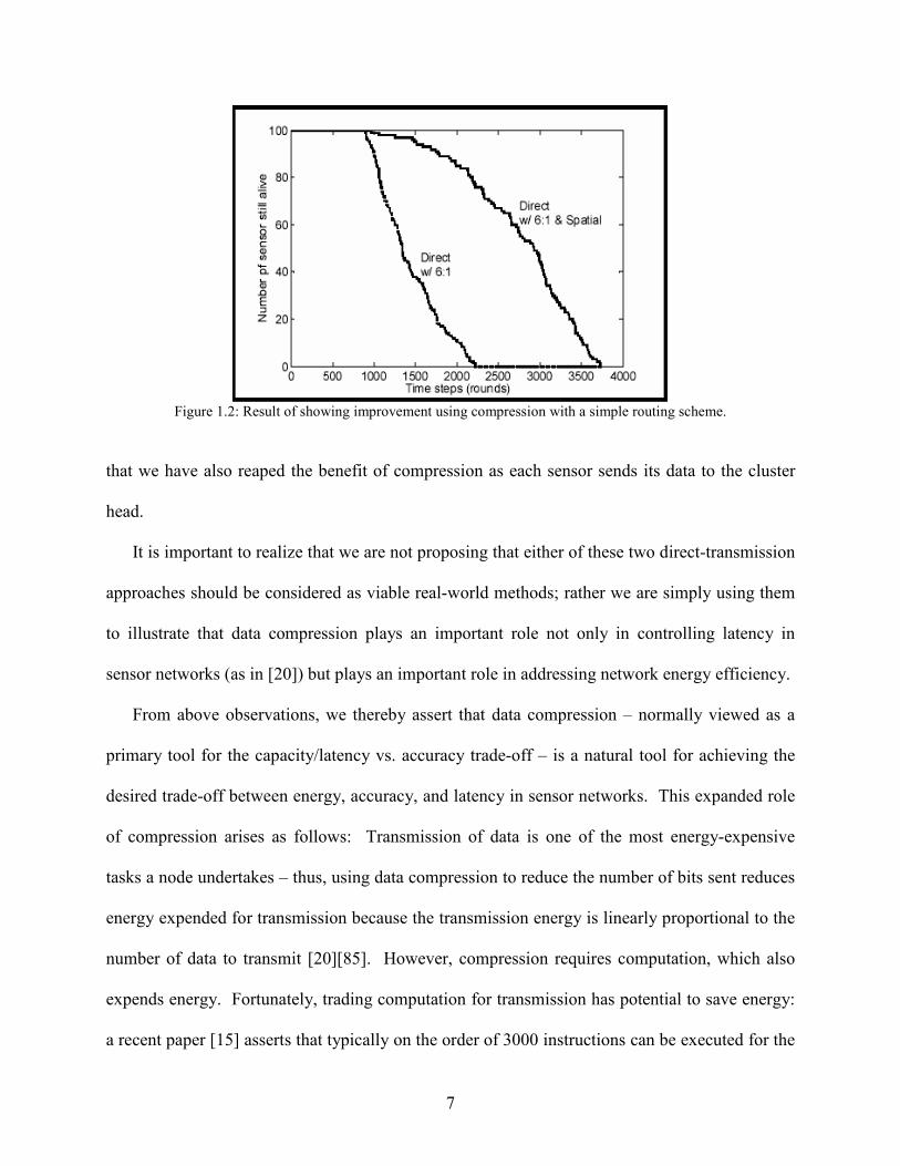
7

Figure 1.2: Result of showing improvement using compression with a simple routing scheme.

that we have also reaped the benefit of compression as each sensor sends its data to the cluster

head.

It is important to realize that we are not proposing that either of these two direct-transmission

approaches should be considered as viable real-world methods; rather we are simply using them

to illustrate that data compression plays an important role not only in controlling latency in

sensor networks (as in [20]) but plays an important role in addressing network energy efficiency.

From above observations, we thereby assert that data compression – normally viewed as a

primary tool for the capacity/latency vs. accuracy trade-off – is a natural tool for achieving the

desired trade-off between energy, accuracy, and latency in sensor networks. This expanded role

of compression arises as follows: Transmission of data is one of the most energy-expensive

tasks a node undertakes – thus, using data compression to reduce the number of bits sent reduces

energy expended for transmission because the transmission energy is linearly proportional to the

number of data to transmit [20][85]. However, compression requires computation, which also

expends energy. Fortunately, trading computation for transmission has potential to save energy:

a recent paper [15] asserts that typically on the order of 3000 instructions can be executed for the

8

energy cost required to transmit one bit over a distance of 100 m by radio – thus, the trade favors

spending computation to reduce the amount of transmission needed.

C. Rate-Energy-Accuracy function for Sensor Network Compression

Classical data compression theory relies on tradeoffs between rate (R) and distortion (D) in

terms of a R-D function. Rate is usually measured in terms of bits/sample and distortion is often

measured as a mean square error between the original and reconstructed signal. In the classical

view, rate impacts latency and distortion impacts the accuracy of the signal reconstruction. As

we explored above, in sensor networks the rate can also impact energy efficiency. Thus, for

sensor networks we propose the use of a 3-D extended version of the R-D function: the Rate-

Energy-Accuracy (R-E-A) function. The rate axis equals the length of compressed data and the

accuracy axis is proportional to distortion caused by compression and reflects the effect of the

compression on the final use of the data while the energy axis assesses the total energy

(compression energy and transmission energy) needed to move the compressed data to the

desired destination. Clearly, decreasing the rate decreases the amount of transmission energy

spent and the duration of transmission time but a decreased rate comes at the expense of

computational energy and time from compression algorithms. A simple characterization of this is

)()()( RERERE TC +=∆ , (1.1a)

)()()( RTRTRT TC +=∆ , (1.1b)

where )(RE∆ and )(RT∆ are the changes in energy and time respectively due to compression to

a rate of R, )(REC and )(RTc are the computational energy and time used to compress to R,

similarly, )(RET and )(RTT are the energy and time needed to transmit at the rate R,

respectively. To maintain certain accuracy (quality of information), if R decreases, both )(REC

and )(RTc increase (better compression requires more computation), in the meantime,

9

)(RET and )(RTT decreases (more compression requires less transmission). Clearly, these

measures depend on the computational efficiency of the compression algorithm, the energy

efficiency of the computational architecture, and the energy efficiency of the transmission

hardware. If we can specify a desired operating point in R-E-A space, then we develop

compression algorithms (as well as low-power computing & transmitting architectures) that

achieve it. However, optimizing of such multi-objective functions (1.1) should be based on the

trinity of compression algorithm, hardware architecture and transmission, which is a horrible task

even if it seems possible in theory. An alternative way to balance the trade-off between

)(RET and )(REC (or )(RTT and )(RTC ) is to apply the idea of separate optimality as in

communication [1]. More specifically, for a given rate, we can choose to maximize the accuracy

using the compression algorithm which is as efficient as possible (minimizing the computation).

1.3 Compression for Inference Tasks in Wireless Sensor Networks

The primary task of sensor networks is to make statistical inferences based on the data

collected throughout the network, it is important to design compression methods that cause

minimal degradation of the accuracy of these inferences. Traditionally, the mean-square-error

(MSE) is the primary distortion measure to guide the compression algorithms in literature. MSE

is a natural choice of the distortion measures for the application whose goal is to reconstruct the

data as near to the original data as possible. However, MSE is not able to capture the effect of the

compression error on the final use of the data – namely, the making of statistical inferences. For

example, if the inference task is estimation, then the accuracy measure should capture the impact

of the compression on the estimation accuracy instead of the reconstruction accuracy.

Compression with the goal to maximize the inference task accuracy must be found instead. The

key to addressing this question is to use distortion measures that accurately reflect the ultimate

10

performance on the tasks. For estimation tasks the ultimate performance is the variance of the

estimation error (at least in the unbiased estimate case) and MSE is only part of what determines

the variance. Similarly, for decision tasks the ultimate performance is probability of detection.

To design compression algorithms with respect to these performance goals it is essential to have

appropriate, tractable metrics that measure the impact of reducing the rate on the inference

performance. For estimation we propose using the Fisher Information Matrix (FIM) to provide a

guide to how to reduce the rate while minimizing the impact on estimation performance. For

decision we propose exploring the use of the Chernoff distance to derive the distortion measures

for the compression algorithms [21]-[28], [60], [75].

Data compression for distributed multi-sensor systems previously considered in the literature

(See the details in Chapter 3) all hold the view that multiple sensors encode received signals and

transfer the coded data directly to a central inference base station. Thus, these prior results are

not made in a true sensor network context. For example, they don’t consider the energy

constraint as mentioned above. Nor do they consider the impact and needs of inter-sensor

communication and cooperation. An even more important aspect not considered in these

previous results is that sensor networks may have multiple inference tasks to accomplish (either

simultaneously or sequentially). Multiple inferences may have conflicting compression

requirements and finding the right way to balance these conflicts is crucial. Thus, another of our

assertions is that compression for sensor networks must consider the case of multiple inferences.

In a sensor network there are a lot of cases where inference tasks are naturally done

sequentially and therefore the sharing of data to complete those tasks can also occur sequentially.

As an example of multiple inferences, consider the case where a sensor network is deployed to

detect and then locate vehicles. This is a case of multiple sequential inferences where the

11

compression can be done sequentially as well. For example, at first sensors might share their

collected data for the purpose of improved detection. After detecting the presence of a vehicle,

data would be shared among sensors to estimate the vehicle’s position, direction and velocity.

Our proposed viewpoint for a novel approach to such a compression scenario is what we call

task-embedded compression: at each task stage, send only that data needed to supplement the

already-delivered data for optimal processing for the current task. For example, (i) the data

stream that is shared during the detection phase is optimally compressed for detection, then (ii)

the data stream that is shared during the estimation phase is the additional data “layer” needed to

perform optimal estimate. It should be pointed out that in the last task of this example there

might be simultaneous multiple inferences (estimate position and velocity) that may very well

have conflicting data compression requirements – thus, we must find ways to compress data that

allow the proper trade-off in this conflict. The key tools we bring to bear on this area are: (i) the

use of multiple distortion measures that are designed to assess the quality of data subsets for use

in the multiple inferences, and (ii) the use of numerical optimization methods to achieve desired

trade-offs based on these quality assessments.

This dissertation is organized as follows. In Chapter 2, we review the basic elements of

inference tasks (estimation and detection) and the framework of compression (transform coding).

In Chapter 3, we first limit our attention to the single inference task case and propose using

Fisher information and Chernoff distance to derive the effective distortion measures for

estimation and detection task respectively. In Chapter 4, we attack optimization of compression

for the general simultaneous multi-parameter estimation problem and simultaneous multi-

inference tasks (joint detection/estimation). In Chapter 5 we consider a sequence of inference

12

tasks. Chapter 6 presents conclusions from this work. Some mathematical deduction needed for

the body of the dissertation and some supplemental materials are in Appendices.

13

CHAPTER 2

Overview of Compression System for Inference Tasks

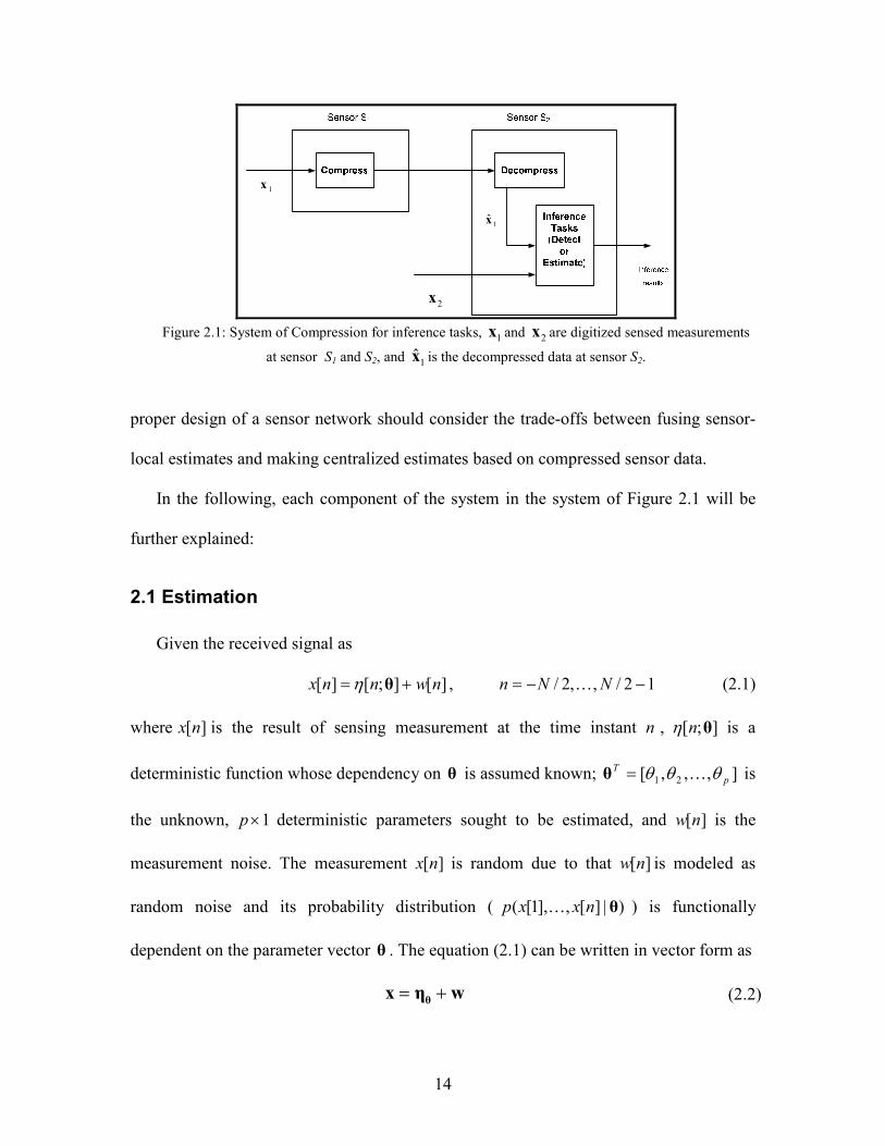
The overall nature of the transportation of sensed data can be vastly different for

different scenarios; however all share one common thread: sending data collected in one

place to some other place where it is processed. As illustrated in Figure 2.1, for the work

we report in this dissertation, we limited our focus on the compression of data received at

one sensor node (S1), which is then transmitted to a second node (S2) where it is

combined with data received locally at S2 to obtain some estimates of some desired

environmental parameters that is reflected in the data or to make some decision of the

presence of anomalies from the data. This scenario is likely to occur as data is routed

through a micro-sensor network; it also is common in macro-sensor networks. Our

approach can also be applied to the case where the data at multiple sensors must be

compressed and transmitted to a central node where estimation is done; We are

particularly (although not exclusively) interested in one aspect of cooperative signal

processing where it is not possible to perform an inference (detection or estimation)

based on a single sensor’s data (e.g., centralized detection, source location), because in

scenarios where it is possible for each sensor to make an inference it is likely to be more

efficient to transmit sensor-local inference results that are then fused (decentralized

system). However, it is generally the case that better inferences can be made when the

fusion center has access to the raw data rather than sensor-local estimates; thus, the

14

1x

1x

2x

Figure 2.1: System of Compression for inference tasks, 1x and 2x are digitized sensed measurements

at sensor S1 and S2, and 1x is the decompressed data at sensor S2.

proper design of a sensor network should consider the trade-offs between fusing sensor-

local estimates and making centralized estimates based on compressed sensor data.

In the following, each component of the system in the system of Figure 2.1 will be

further explained:

2.1 Estimation

Given the received signal as

][];[][ nwnnx += θη , 12/,,2/ −−= NNn K (2.1)

where ][nx is the result of sensing measurement at the time instant n , ];[ θnη is a

deterministic function whose dependency on θ is assumed known; ],,,[ 21 p

T θθθ K=θ is

the unknown, 1×p deterministic parameters sought to be estimated, and ][nw is the

measurement noise. The measurement ][nx is random due to that ][nw is modeled as

random noise and its probability distribution ( )|][,],1[( θnxxp K ) is functionally

dependent on the parameter vector θ . The equation (2.1) can be written in vector form as

wηx θ += (2.2)

15

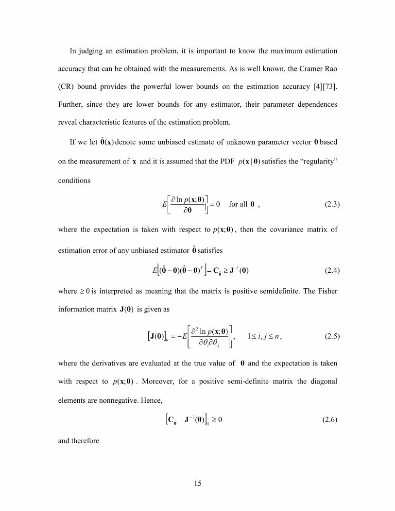
In judging an estimation problem, it is important to know the maximum estimation

accuracy that can be obtained with the measurements. As is well known, the Cramer Rao

(CR) bound provides the powerful lower bounds on the estimation accuracy [4][73].

Further, since they are lower bounds for any estimator, their parameter dependences

reveal characteristic features of the estimation problem.

If we let )(ˆ xθ denote some unbiased estimate of unknown parameter vector θ based

on the measurement of x and it is assumed that the PDF )|( θxp satisfies the “regularity”

conditions

0);(ln

=

∂

∂θ

θxpE for all θ , (2.3)

where the expectation is taken with respect to );( θxp , then the covariance matrix of

estimation error of any unbiased estimator θ satisfies

[ ] )()ˆ)(ˆ( 1ˆ θJCθθθθθ

−≥=−− TE (2.4)

where 0≥ is interpreted as meaning that the matrix is positive semidefinite. The Fisher

information matrix )(θJ is given as

[ ]

∂∂∂

−=ji

ij

pE

θθ);(ln

)(2 θx

θJ , nji ≤≤ ,1 , (2.5)

where the derivatives are evaluated at the true value of θ and the expectation is taken

with respect to );( θxp . Moreover, for a positive semi-definite matrix the diagonal

elements are nonnegative. Hence,

[ ] 0)(1ˆ ≥− −

iiθJC

θ (2.6)

and therefore

16

[ ] [ ]iiiii )()ˆvar( 1

ˆ θJCθθ

−≥= (2.7)

Whenever it is desired to estimate )g(θα = for g , an r -dimensional function, then,

0)g(

)()g( 1

ˆ ≥∂

∂∂

∂− −

θ

θθJ

θ

θC

T

α , (2.8)

where

∂∂

∂∂

∂∂

∂∂

∂∂

∂∂

∂∂

∂∂

∂∂

=∂

∂

p

rrr

p

p

ggg

ggg

ggg

θθ

θθ

θθ

θθ

θθ

θθ

θθ

θθ

θθ

)()()(

)()()(

)()()(

)g(

21

2

2

2

1

2

1

2

1

1

1

L

MOMM

L

L

θ

θ.

Geometrically, the covariance matrix θ

C ˆ can be visualized in the space of the

estimation error by the concentration ellipsoid

κ=−− − )ˆ()ˆ( 1ˆ θθCθθθ

T (2.9)

where κ is a constant that determines the size of the p-dimensional region enclosed by

the surface. In these terms an equivalent formulation of the CR inequality reads: For any

unbiased estimate of θ the concentration ellipsoid (2.9) lies inside or on the bound

ellipsoid defined by

κ=−− )ˆ()ˆ( θθJθθ T . (2.10)

The size and orientation of the ellipsoid (2.10) can be best described in terms of the

eigenvalues and eigenvectors of the symmetric pp× matrix J . To this end the

eigenvalue problem

iii ςJς λ= , pi ,,1K= , (2.11)

17

has to be solved, where 1λ ,…, pλ are eigenvalues of J and pςς ,...,1 the corresponding

eigenvectors. The mutually orthogonal eigenvectors coincide with the principal axes of

the bound ellipsoid and form an orthogonal matrix ( )pςςA ,,1 K= that diagonalize J

=

n

T

λ

λ

0

01

OJAA . (2.12)

Thus, rotating the coordinate axes by means of the transformation TA in the new

variables defined by

)ˆ( θθAξ −= T . (2.13)

then the ellipsoid (2.13) takes the form

κλ ==−− ∑=

n

i

ii

T

1

2)ˆ()ˆ( ςθθJθθ . (2.14)

This is in the coordinates iς the equation of an ellipsoid in its standard form with

semiaxes of length iλκ / . The bigger iλ , the more accurate on this semiaxis iς , on the

contrary, the smaller iλ , the wider estimation error range will be, if 0=iλ , then the

value of the corresponding coordinate iς can be chosen arbitrarily, i.e. (2.14) describes a

degenerate ellipsoid extending to infinity in this coordinate direction. The Fisher

information matrix exhibits the information content of the estimation problem. Thus,

physically 0=iλ means that there is no information at all about the corresponding

coordinate iς , i.e., iς is unobservable.

CR can not only provide us an intuitive understanding and a deeper insight into the

compression for estimation problem by investigating the influence of compression

18

(selection or quantization) on the estimation accuracy, but also CR is asymptotically

achievable by taking the maximum likelihood estimation (MLE) as estimation procedure.

The MLE for a vector parameter θ is defined to be the value that maximizes the

likelihood function );( θxp over the allowable domain for θ . Assuming a differentiable

likelihood function, the MLE is found from

0);(ln

ˆ

=∂

∂

= ML

p

θθ

θx

θ, (2.15)

If we let mθ designate the maximum-likelihood estimate of θ based on N i.i.d. random

variables and 0θ be the true value of the parameter, mθ converges in law (also called

convergence in distribution) to a normal random variable: That is

law

m YN →− )ˆ( 0θθ . (2.16)

where

))(,0(~ 0

1 θJ −NY . (2.17)

The ML estimate mθ is asymptotically efficient in the sense that asymptotically it attains

the Cramer-Rao lower bound as ∞→N .

2.2 Detection

Detection can be formulated as a binary statistical hypothesis test. If 0H and 1H refer

to the hypotheses that the target is absent or present, respectively, we have

),(~

)(~

11

00

θxx

xx

pH

pH, (2.18)

19

where 0H and 1H have nonzero priori probabilities 0P and 1P , respectively. Under

hypothesis 0H and 1H , x is distributed according to the pdf’s 0p and 1p . Besides a

function of x , 1p is also dependent on the parameter vector θ . The likelihood ratio

)(/)()( 01 xθx,x ppL = is a sufficient statistic for detection, i.e., all we need to know is

the likelihood ratio for deciding between the hypotheses 0H and 1H . When the

parameter vector θ is unknown, the generalized likelihood ratio is usually applied by

replacing θ with its MLE (2.15). In the subsequent equations in this section, θ is

omitted for the simplicity. The likelihood ratio is invariant to invertible operations such

as the transform in the transform coder discussed in the next section.

Under a variety of optimality criteria, the detection algorithms take the form of an

LRT

τ

0

1

)(

)()(

0

1

H

H

p

pL

<

>=

x

xx . (2.19)

where τ is an appropriate threshold. The value of τ depends on the optimality criterion.

In a Neyman-Pearson test, the threshold τ is chosen such that, for a given probability of

false alarm ( ))((0 τ>= xLpPf , the probability of miss ( ))((1 τ<= xLpPmiss ) is

minimized, or for a given missP , fP is minimized. Under the minimum-probability-of-

error rule (Bayes rule), the optimal decision is [ ] [ ])(maxarg|maxargˆ xx iiiii pPHPi == ,

where iP is priori probability for hypothesis iH . The LRT in (2.19) is then optimal when

τ is equal to the ratio 10 / PP of the priori probabilities. The probability of error in this

case is

20

xxx dpPpPPe ∫= ))(),(min( 1100 . (2.20)

The problem of choosing an optimal decision rule is treated in a broad literature [5],

relatively small attention is paid to how to quantify the discriminating ability of data on

the detection performance. The discriminating ability of data (or the performance of the

detection) can be evaluated through the Chernoff distance. Chernoff distance gives an

upper bound on both fP and missP :

))(),(( 10 xx pps

fseP

µτ −−≤ , (2.21)

))(),((1 10 xx pps

missseP

µτ −−≤ , (2.22)

where sµ is the Chernoff distance defined by:

xx

xxxx d

p

ppppµ

s

s

−= ∫ )(

)()(ln))(),((

0

1010 , 10 << s . (2.23)

and τ is the threshold in the LRT of (2.19). When the Bayes rule is applied, 10 / PP=τ

and (2.20) together with the fact that 10,),min( 1 ≤≤≤ − sbaba ss , give an upper bound

on eP

))(),((

1

1

010 xx ppss

esePPP

µ−−≤ . (2.24)

The bound is very tight within a scale factor [49][73]. The Chernoff bounds (2.21), (2.22),

and (2.24) on fP , missP , and eP hold for any distribution of the data and any sample size

N .

2.3 Data Compression and Decompression

Data compression methods are commonly developed either under a classical rate-

distortion viewpoint [1] or an operational rate-distortion viewpoint [11],[29]. The

21

classical viewpoint strives to develop methods that are optimal on average, over an

ensemble of realizations of a random process model; this necessarily demands a random

model for the signal and knowledge of a probability structure. The operational viewpoint

specifies a compression framework (whose design is often based on insights from the

classical viewpoint) and then optimizes the operating point of that framework for the

particular signal at hand; this has the advantage of relaxing the assumptions made on the

signal (e.g., can assume it is deterministic) but has the disadvantage that side information

describing the operating point must be included as overhead in the compressed bit stream.

Because a sensor network would likely be required to operate in an abundance of

differing signal environments, in this dissertation, we focus on the operational viewpoint

to remove the necessity of assuming (limiting) statistical models for the signal. Typically,

the operational framework uses numerically computable allocations of rates resources

(see [29], [33]) rather than classical closed forms such as reverse water-filling [1].

Moreover, we discuss compression under the umbrella of transform-based coders,

which are ubiquitous in practice. The choice of transform coding is due to (i) it provides

us the rigid theoretical analysis and design of optimal compression for detection and

estimation tasks; (ii) it provides us good compression performance and low

computational complexity [31][32] because the performance of compression is

proportional to the time consumed and hardware complexity of compression algorithm

and transform coding provides us the best tradeoff in the energy-rate-accuracy space, i.e.,

transform coding can achieve a given certain compression performance in a more

efficient way than other compression schemes.

22

)(xy T= )(yq Q= )(qc C=

)(1 cq −= C)(~

ˆ 1 qy −= Q)ˆ(ˆ 1 yx −= Tx

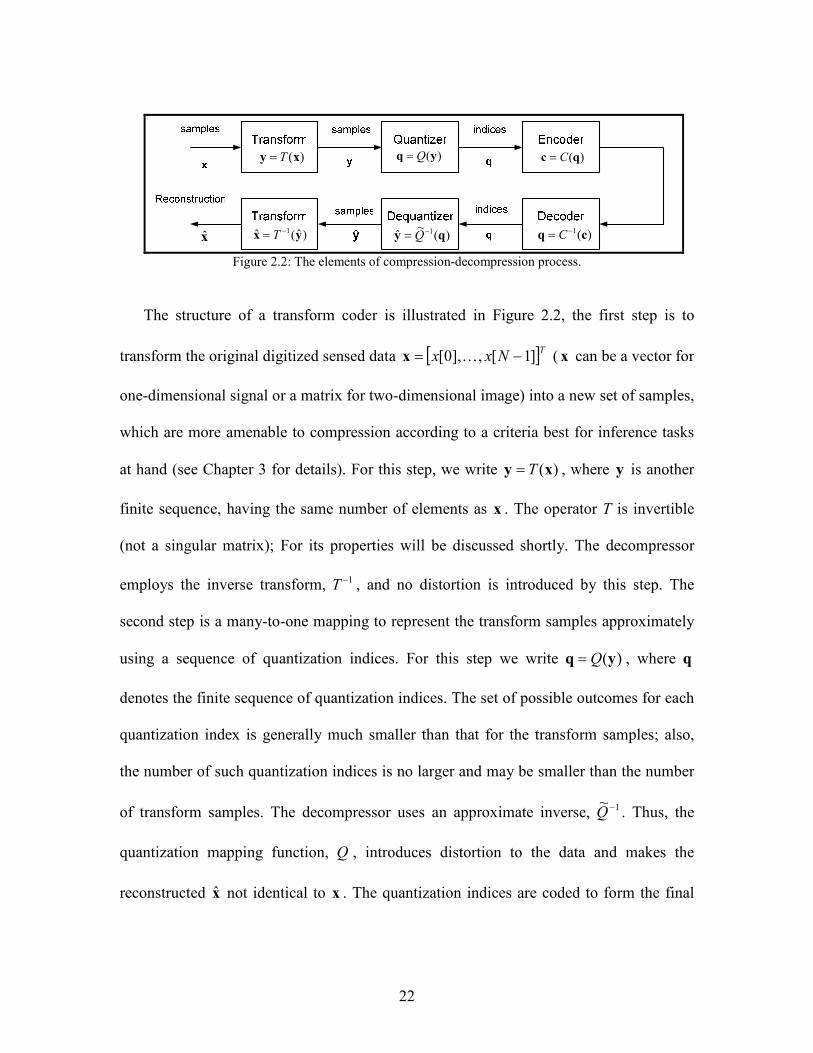
Figure 2.2: The elements of compression-decompression process.

The structure of a transform coder is illustrated in Figure 2.2, the first step is to

transform the original digitized sensed data [ ]TNxx ]1[,],0[ −= Kx (x can be a vector for

one-dimensional signal or a matrix for two-dimensional image) into a new set of samples,

which are more amenable to compression according to a criteria best for inference tasks

at hand (see Chapter 3 for details). For this step, we write )(xy T= , where y is another

finite sequence, having the same number of elements as x . The operator T is invertible

(not a singular matrix); For its properties will be discussed shortly. The decompressor

employs the inverse transform, 1−T , and no distortion is introduced by this step. The

second step is a many-to-one mapping to represent the transform samples approximately

using a sequence of quantization indices. For this step we write )(yq Q= , where q

denotes the finite sequence of quantization indices. The set of possible outcomes for each

quantization index is generally much smaller than that for the transform samples; also,

the number of such quantization indices is no larger and may be smaller than the number

of transform samples. The decompressor uses an approximate inverse, 1~ −Q . Thus, the

quantization mapping function, Q , introduces distortion to the data and makes the

reconstructed x not identical to x . The quantization indices are coded to form the final

23

bit-stream. We write )(qc C= . This step is invertible and introduces no distortion so that

the decompressor may recover the quantization indices as )(1 cq −= C .

2.3.1 Coding

The purpose of coding is to exploit statistical redundancy among the quantization

indices. The quantization and transform elements are designed in such a way as to ensure

that the redundancy is localized. Ideally, the underlying random variables are all

statistically independent. In that case, the indices may be coded independently and the

only form of statistical redundancy which need be considered is that associated with any

non-uniformity in their probability distribution.

2.3.2 Transforms

The transform is responsible for mapping the original samples into a form which

enables comparatively simple quantization and coding operations. On the one hand, the

transform should capture the essence of statistical dependencies among the original

samples so that the group of adjacent transform samples and the quantization indices

possess common characteristics and exhibit at most only very local dependencies, ideally,

independent; On the other hand, the transform should separate irrelevant information

from relevant information according to certain criteria so that the irrelevant samples can

be identified and quantized more heavily or even discarded whereas relevant samples are

quantized lightly.

We can consider an NN × linear transform matrix A , which maps an N-dimensional

input vector, x , into an N -dimensional output vector, y , according to

Axy = . (2.25)

Here, we restrict our attention to invertible transforms, writing the inverse as

24

Syx =1 , (2.26)

where S is the inverse of A ; i.e., ISA = , the NN × identity matrix. In this case, S is

the unique inverse of A , which we may write as

AS =−1 , or 1−= AS . (2.27)

Observe that the transform coefficients may be expressed as

xa qqy = , 1,,1,0 −= Nq K . (2.28)

where qa is the q th column of the nn× matrix, A . We refer to qa as the thq “analysis

vector,” since it “analyzes” the original vector x , to determine its thq transform

coefficient. Accordingly, we refer to A as the analysis matrix. Also, the inverse

transform may be expressed as

∑−

=

=1

0

1

n

q

qqy sx , (2.29)

where qs is the thq column of the nn× matrix, S . We refer to qs as the thq “synthesis

vector,” since 1x is “synthesized” from a linear combination of the qs , with the transform

coefficients serving as the weights. Accordingly, the matrix,S , is known as the “synthesis

matrix”.

A transform is said to be orthonormal if the analysis vectors are all mutually

orthogonal and have unit norm (length); i.e.,

0=jH

i aa , ji ≠∀ , (2.30a)

12== ii

H

i aaa , i∀ (2.30b)

This means that IAAAA == HH , so that HAS = is a unitary matrix. Equivalently, the

analysis and synthesis vectors for orthonormal transforms are identical. An orthonormal

25

transform performs an orthonormal expansion of the input signal as the sum of its

projections onto each of the basis vectors; i.e.,

( )∑∑ ⋅==q

qq

H

q

qqy ssxsx . (2.31)

An important property of orthonormal transforms/expansions is that they are “energy

preserving,” meaning that

22

,

*

22

yss

ssxxx

===

===

∑∑

∑∑∑

q

q

ji

j

H

iji

j

jj

i

H

ii

H

p

p

yyy

yyx

. (2.32)

In words, the sum of the squares of the input samples (energy of the input), is identical to

the sum of the squares of the transform coefficients (energy of the output). This property

is often known as Parseval’s relation.

To appreciate the significance of this property for compression, consider the

compression system of Transform Coding Structure. Let yye ˆ−=y denote the error

introduced into the transform coefficients by quantization. Similarly, let 11 xxe −=x

denote the error introduced into the reconstructed samples by the entire compression

system. By linearity of the transform, yx See = and if the transform is orthonormal,

22

yx ee = . In words, the error energy in the samples is identical to the error energy in

the transform coefficients. Minimizing the mean square error (MSE) of the quantized

transform coefficients is then identical to minimizing the MSE of the reconstructed

samples. The use of an orthonormal transform has no impact on the rate-distortion

function and the selection of an “ideal” transform ensures that the transform bands may

be quantized and coded independently without penalty.

26

0x 1x 2x

2t 3t 1−Mt

1ˆ −Mx

1t x

Figure 2.3: Graphical representation of scalar quantization.

2.3.3 Quantization

Quantization is the element of lossy compression systems responsible for reducing

the precision of data (reduce the wordlength of samples) in order to make them more

compressible. In most lossy compression systems, quantization is the sole source of

distortion. Next, the most widely used quantization (scalar quantization) will be reviewed.

Scalar quantization (SQ) is the simplest of all lossy compression schemes. It can be

described as a function that maps each element in a subset of the real line to a single

value in that subset. Consider partitioning the real line into M disjoint intervals

[ )1, += qqq ttI , 1,,1,0 −= Mq K . (2.33)

with

+∞=<<<=∞− Mttt L10 .

Within each interval, a point qx is selected as the output value (or codeword) of qI .

The process of scalar quantization is illustrated in Figure 2.3. A scalar quantizer is

basically a mapping from continuous ℜ to discrete 1,,1,0 −MK . Specifically, for a

given x , )(xQ is the index q of the interval qI which contains x . The dequantizer is

given by

qxqQ ˆ)(~ 1 =−

27

when ),[ 1+=∈ qqq ttIx , that is qxxQQ ˆ))((~ 1 =− . Clearly, the qt can be thought of as

thresholds, or decision boundaries for the qx . The size of the quantization index set is

constant, M , therefore only M2log bits will be needed to signal the codeword chosen

by the quantizer, which is why a SQ that has bM 2= boundaries is often called b-bit

quantizer. There are a number of scalar quantizers (such as uniform quantizer, Lloyd-

max scalar quantizer, entropy coded scalar quantization) which differ in the choice of the

boundaries qt and the reconstruction value qx . For example, for uniform quantization [10]

the decision boundaries are spaced evenly, except for the two outer intervals, the

reconstruction values are also spaced evenly, with the same spacing as the decision

boundaries: in the inner intervals, they are the midpoints of the intervals. One of the most

used uniform quantizer is the midrise quantizer that can be represented as

2

)(∆

+

∆

∆=x

xQ ,

Here, ∆ denotes the step size and ⋅ denotes an operator that rounds downwards to

the nearest integer. Different from the uniform quantizer, the Lloyd-Max quantizer

[10][11] sets the decision boundaries and reconstruction values to minimize MSE

between the input samples and reconstructed values subject to the size of the code (M)

according to the probability density function (PDF) of the samples. The entropy coded

scalar quantizer [11] minimizes MSE subject to a constraint on the entropy of the

quantization indices. No matter what type of quantizer, for the high rates (M is large or

the number of bits of quantizer is large1) and the data is individually independent

1 The large is a loose concept, one or two bits could be called large, see [31][32]

28

distributed (IID), the distortion-rate function, or quantization noise power, can be

modeled in the form of

bCbd 22 2)( −≅ σ . (2.34)

where 2σ is the variance of the samples and C is a constant which is different for

different quantizers [11][30], and is usually determined heuristically in most cases.

A very desirable feature of compression schemes is the ability to successively refine

the reconstructed data as the bit-stream is decoded. In this situation, a (perhaps crude)

representation of the data to be compressed becomes available after decoding only a

beginning small subset of the compressed bit-stream for one purpose. As more of the

compressed bit-stream is decoded, the representation of data can be improved

incrementally for another purpose. Compression systems possessing this property are

facilitated by embedded quantization and this is the basis for the compression for

sequential task embedded tasks introduced in Chapter 1.

In embedded quantization, the intervals of higher rate quantizers are embedded within

the intervals of lower rate quantizers. Equivalently, the intervals of lower rate quantizers

are partitioned to yield the intervals of higher rate quantizers. Consider a sequence of

K embedded scalar quantizers 0Q , 1Q , 2Q , …, 1−KQ . The intervals of 1−KQ are then

embedded within the intervals of 2−KQ , which in turn are embedded within those of 3−KQ ,

and so on. Equivalently, the intervals of 0Q are partitioned to get the intervals of 1Q ,

which in turn are partitioned to get the intervals of 2Q , and so on.

Specifically, each interval of 0Q ( 1,,1,0 000−= MqIq K ) is partitioned into 1M

intervals 10 ,qqI 1,,1,0 10 −= Mq K . The total number of intervals of 1Q is then 10MM .

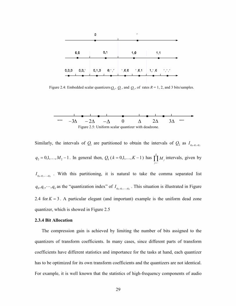
29

Figure 2.4: Embedded scalar quantizers

0Q , 1Q , and

2Q , of rates R = 1, 2, and 3 bits/samples.

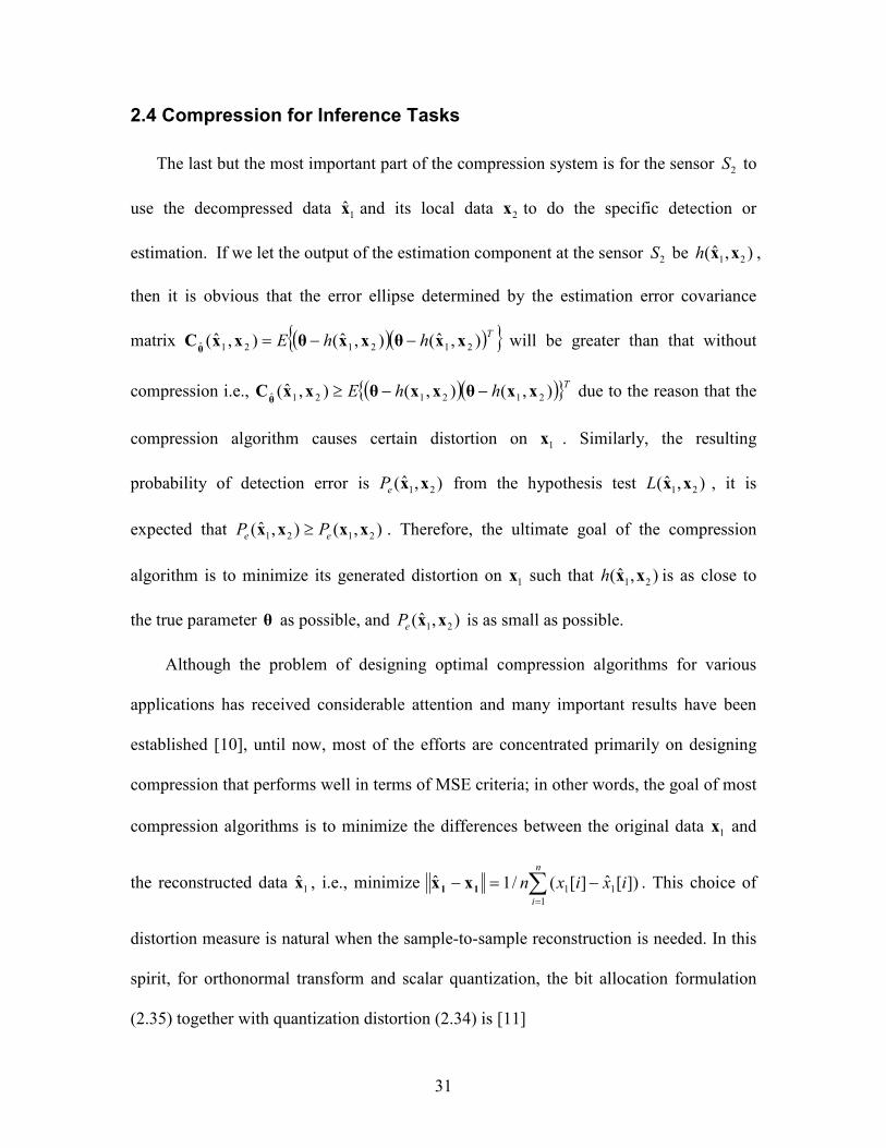
∆− 0 ∆∆−3 ∆3∆− 2 ∆2 Figure 2.5: Uniform scalar quantizer with deadzone.

Similarly, the intervals of 1Q are partitioned to obtain the intervals of 2Q as 210 ,, qqqI

1,,1,0 22 −= Mq K . In general then, kQ ( 1,,1,0 −= Kk K ) has ∏−=

k

j

jM intervals, given by

kqqqI ,,, 10 K. With this partitioning, it is natural to take the comma separated list

kqqq ,,, 10 L as the “quantization index” of kqqqI ,,, 10 K

. This situation is illustrated in Figure

2.4 for 3=K . A particular elegant (and important) example is the uniform dead zone

quantizer, which is showed in Figure 2.5

2.3.4 Bit Allocation

The compression gain is achieved by limiting the number of bits assigned to the

quantizers of transform coefficients. In many cases, since different parts of transform

coefficients have different statistics and importance for the tasks at hand, each quantizer

has to be optimized for its own transform coefficients and the quantizers are not identical.

For example, it is well known that the statistics of high-frequency components of audio

30

are significantly different from those of the lower frequency components, therefore a

subband coder (audio MP3 coder [74]) assigned different quantizer to different spectral

bands of audio. The optimal bit allocation (or operational rate distortion optimization for

a particular signal at hand instead of classical operational rate distortion optimization for

an ensemble of realizations of a random process models) can be formulated as: First,

transform coefficients are grouped into M coding units where each coding unit can be

quantized by K different available quantizers. For each coding unit i quantized by a

quantizer j, we have an average number bits per coefficient ijr for coding unit i and the

corresponding distortion ijd caused by the quantizer j . We make no assumptions of any

particular structure for the ijr and ijd ; we simply use the convention that quantization

indices are listed in order of increasing “coarseness”; i.e. 1=j is the final quantizer

(highest 1ir and lowest 1id ) and Kj = is coarsest. We consider here that the distortion 1id

due to 1ir is known, or it is possible to replace measured ijr and ijd by values that are

estimated on models, but this would not affect the bit allocation algorithm. We then

define an objective distortion function )(⋅f that is a function of ijd and optimize it under

the constraint that the total number of bits is upper bounded by the budget TR .

Mathematically speaking, the goal of bit allocation is to find the optimal quantizer *

ib for

each coding unit i such that

T

N

iib

Rri

≤∑=1

* (2.35)

and the specified form of distortion measure ( )**2

*1

,,,21 NNbbb

dddf K is optimized.

31

2.4 Compression for Inference Tasks

The last but the most important part of the compression system is for the sensor 2S to

use the decompressed data 1x and its local data 2x to do the specific detection or

estimation. If we let the output of the estimation component at the sensor 2S be ),ˆ( 21 xxh ,

then it is obvious that the error ellipse determined by the estimation error covariance

matrix ( )( ) ThhE ),ˆ(),ˆ(),ˆ( 212121ˆ xxθxxθxxCθ

−−= will be greater than that without

compression i.e., ( )( ) ThhE ),(),(),ˆ( 212121ˆ xxθxxθxxCθ

−−≥ due to the reason that the

compression algorithm causes certain distortion on 1x . Similarly, the resulting

probability of detection error is ),ˆ( 21 xxeP from the hypothesis test ),ˆ( 21 xxL , it is

expected that ),(),ˆ( 2121 xxxx ee PP ≥ . Therefore, the ultimate goal of the compression

algorithm is to minimize its generated distortion on 1x such that ),ˆ( 21 xxh is as close to

the true parameter θ as possible, and ),ˆ( 21 xxeP is as small as possible.

Although the problem of designing optimal compression algorithms for various

applications has received considerable attention and many important results have been

established [10], until now, most of the efforts are concentrated primarily on designing

compression that performs well in terms of MSE criteria; in other words, the goal of most

compression algorithms is to minimize the differences between the original data 1x and

the reconstructed data 1x , i.e., minimize ∑=

−=−n

i

ixixn1

11 ])[ˆ][(/1ˆ11 xx . This choice of

distortion measure is natural when the sample-to-sample reconstruction is needed. In this

spirit, for orthonormal transform and scalar quantization, the bit allocation formulation

(2.35) together with quantization distortion (2.34) is [11]

32

( ) ∑=

−=

M

i

r

iiiNbbb

iib

N

Cdddf1

22

2)1

*

**2

*1

2,,, σηK (2.36)

where iC is a constant determined by the ON transform and SQ quantizer used and iη

denotes the ratio between the number of coefficients in the coding unit i and the total

number of coefficients, and 2

iσ is the variance the coding unit i. The value of iσ is

usually estimated from the coefficients in unit i. According to [11], (2.36) can be

extended to the more complex quantizer, such as vector quantizers. The classical

compression methods for non audio/video signals are typically based on (2.36); even for

audio/video, (2.36) is also the primary choice of distortion function [29]. However, when

compression algorithms are studied as an element of an inference system, for estimation

tasks the ultimate performance measure should be the variance of the estimation error,

i.,e., ),ˆ( 21ˆ xxCx , and similarly, for detection tasks the ultimate performance measure

should be the probability of detection error, i.e., ),ˆ( 21 xxeP . MSE is not only

inappropriate since it is weakly related to xC ˆ and eP , but is not required because

inference accuracy, not reconstruction of signal, is the primary objective. Therefore

appropriate, useable metrics that measure the impact of rate reduction on the inference

performance must be found. Besides, we assume that the inference (detection/ estimation)

processing and compression processing are not jointly designed, i.e., the

detection/estimation processing uses methods that are optimal in the absence of

compression and the compression process is optimal for optimal detector or efficient

estimators. Although joint design is preferred from an ultimate optimality perspective, we

believe it is of limited value in the inter-operability environment of practice because

sensor networks are more likely to be called on to provide data to other systems that are

33

Our Compression Framework

Tx

Q1

Q2

QN

T -1 Estimation(Fisher)

Detection

(Chernoff )

0H

1H

1−MH

Reconstruction

θ

“Remote”

Sensor

Data

“Local”

Sensor

Data

Sensor #1Sensor #2

(MSE)

Evaluate

Quality

for Tasks

The Key

to Our

Method!

Figure 2.6 : Framework of the compression method.

independently designed (e.g., “legacy” systems and other “system of systems” scenarios);

Since there are numerous approaches to estimate a parameter or detect a signal, the

compression algorithms must be universal.

The synopsis of our compression framework is summarized as follows: We model

the collected sensor data as a deterministic signal plus additive noise. As illustrated in

Figure 2.6, for simplicity and with its own importance, we seek to compress a block of

data x collected at sensor S1 so that it can be transmitted to S2 using no more than a

budgeted R bits while making the decision about the presence of the signal with the

lowest possible probability of detection error and/or making an estimate θ at S2 (using

the compressed data and S2-local data) with the smallest mean-square estimation error.

34

The processing box label “T” is a linear invertible transform (preferably orthogonal)

whose output coefficients are quantized by the set of quantizers Qi; each coefficient is

evaluated to assess its importance or quality for the desired inference tasks and bits are

allocated to the various quantizers on that basis. We use Fisher information (2.5) to assess

the impact on estimation accuracy and use Chernoff distances (2.23) to assess the impact

on decision accuracy. As will be seen, different inference tasks rely on different sets of

coefficients. If multiple inference tasks are required, it is also crucial to find methods to

properly determine the optimal allocation of the bits to enact the desired trade-offs. The

key part of all cases is finding a method that can be used to assess the coefficients’

quality based on Fisher information and Chernoff distances. We will explore this in detail

in the next Chapter.

35

CHAPTER 3

Data Compression for Parameter Estimation and

Detection

3.1 Fisher-Information-Based Data Compression for Parameter

Estimation

3.1.1 Overview of Previous Work

Data compression for distributed multi-sensor estimation problems has been

previously considered to some degree by many others [34]-[41]. To put our results in

context we briefly review the main results of these researchers. Generally, these results

are cast in the form shown in Figure 3.1. The source emits a signal s(θ ) depending on an

unknown source parameter θ; the ith sensor receives signal )(θiX that is related to s(θ )

and encodes it as )(ˆ θiX , which is transmitted to a central processing center where the

encoded signals are decoded and then used to make an estimate; Figure. 3.1 shows the

estimation of either (i) the parameter θ, or (ii) the signal s(θ ) itself.

These previous results can be grouped in several ways, based on what is being

estimated, what compression framework is used, etc. The focus is either on (i)

optimizing compression for the purpose of estimation of the source signal [16],[17],[34],

[35],[58] or on (ii) optimizing compression for the purpose of estimating the source

parameter [36]-[39],[40],[41]. Many focus on restricting the encoder to being a scalar

quantizer that is then designed according to some optimization criteria [34], [35], [36],

36

Encoder

Decoder

&

Processing

Encoder

EncoderSensor

Source

)(1 θX

)(2 θX

)(θNX

Sensor

Sensor

)(ˆ1 θX

)(ˆ2 θX

)(ˆ θNX

)(θs

)(ˆ

or

ˆ

θ

θ

s

Figure 3.1: Classical set-up for compression in a distributed sensor system.

[38], [39], [41], [58]. Others focus on more general compression structures

[16],[17],[37],[40] , although, most of these ([17],[37],[40]) focus on establishing inform-

ation theoretic results and bounds. Of these, the closest to our approach is the approach

by Lam and Reibman [39], who used the idea of optimizing the compression with respect

to an estimation-centric distortion function (the Cramer-Rao lower bound), but they only

considered scalar quantization of signal samples rather than a more powerful

compression framework like transform coding, as considered here. The results in [41]

take an inference-centric viewpoint, although it chooses a quite different metric driven by

the specific application they considered; their approach seems considerably less general

than that considered here.

3.1.2 Fisher Information for Compression

Fisher information is a well-known concept in estimation theory [4]. It provides a

numerical assessment of how useful a set of data is for estimating a parameter. The

amount of Fisher information that a set of data possesses is proportional to the parameter

estimation accuracy. Its properties include: (i) the Fisher information is invariant under

37

application of invertible maps to the data [78] and is decreased under application of

quantization (Appendix B), (ii) the reciprocal of the Fisher information yields the

Cramer-Rao Lower Bound on the variance of any unbiased parameter estimator, and (iii)

it can be viewed as an “information” measure because it is nonnegative and it is additive

for independent observations (Appendix A). However, it is fundamentally different from

Shannon information, which measures how many bits must be used to represent a signal.

A Shannon-Fisher connection has been explored in [1] in a classical rate-distortion

information-theoretic viewpoint.

Let the real1 data vector x be drawn from a probability density function (PDF) p(x;θ)

that is parameterized by θ, which is to be estimated. The Fisher information (FI) of this

estimation problem is defined to be

( )

∂

∂=

2;ln

);(θ

θθ

xx

pEJ , (3.1)

where the expected value is taken with respect to p(x;θ) and therefore the Fisher

information is not a function of the data vector x. However, the notational dependence

on x shown on the left-hand side of (3.1) is included merely to keep track of the data set

or data subset for which the Fisher information is computed. As indicated on the left-

hand side of (3.1), the Fisher information can be a function of the parameter to be

estimated, although in many cases it is not.

Clearly, compression of the data vector x using a lossy algorithm changes the

underlying PDF to that of the post-compression data x available for estimation, and

therefore alters the Fisher information. More specifically, compression x decreases the

1 Modifications to handle the complex case are straightforward [4].

38

Fisher information (Appendix B). Then, our goal here is to seek operational rate-

distortion methods to maximize the amount of Fisher information remaining in the data

set x while satisfying a budget R on the rate used to represent the data set. However,

when the Fisher information depends on the parameter θ to be estimated a question

arises as to how to precisely characterize our desire to maximize the Fisher information

without knowing at what parameter value we should be concentrating our efforts. Thus,

in general, we propose a minimax approach. Let );( xθJ and )ˆ;( xθJ be the Fisher

information of the original data x and the compressed data x , respectively. The minimax

approach is to compress to R bits such that we satisfy

[ ])ˆ;();(maxminˆ

xxx

θθθ

JJ − , (3.2)

where the maximization is over all the possible parameter values and the minimization is

over all compressed x that meet the bit budget R. Clearly, when the Fisher information

does not depend on the parameter θ or when the Fisher information can be represented

by the product of two independent factor, such as )ˆ()()ˆ;( 21 xx JJJ θθ = , the minimax

approach (3.2) is equivalent to maximizing )ˆ(xJ or )ˆ(2 xJ , which are the cases we will

focus on. There are surely tasks for which the minimax would be needed, but we found

no typical important estimation tasks that required it, and therefore, this general minimax

approach is left for future work.

3.1.3 Compressing to Maximize Fisher Information

Let noisy measurement kx be the set of data collected at sensor node Sk (k = 1, 2) to

support estimation of the parameter θ. We will model the received signal vectors kx as

2,1,)( =+= kkkk wsx θ , (3.3)

39

where )(θks is an unknown deterministic signal vector dependent on the unknown scalar

parameter θ to be estimated, and wk is a additive noise vector with w1 and w2

independent of each other. Without loss of generality, we assume that the noise vector

w1 is white (if not, prewhitening filter [4][5] can be used before compression) and the

variance 21σ of w1 is known from design considerations and/or sensor measurements in

the absence of a signal; the characteristics of w2 is not needed to be known for

developing the compression.

As shown in Figure 2.1 and Figure 2.6, measurement vector 1x will be compressed

at S1 and sent to S2; the decompressed vector 1x is then used with 2x to estimate the

parameter θ. So the general goal of our compression method is as follows, expressed as

transform coding with a Fisher-information-based distortion. Given some orthonormal

(ON) decomposition basis set Nnn 1 =φ (e.g., wavelet transform, DFT, DCT, etc.) we can

write the signal vector to be compressed as

,)(11

1

1

∑∑

∑

==

=

+=

=

N

n

nn

N

n

nn

N

n

nnχ

φφ

φx

ωθξ (3.4)

where nχ are the data coefficients, )(θξn are the parameterized signal coefficients, and

nω are the noise coefficients.

We wish to select which coefficients nχ should be quantized and transmitted to

achieve a desired rate-Fisher information goal. Only those coefficients with significant

contribution to the Fisher information should be selected. The quantization should be

done such that only minimal degradation in Fisher information occurs. Let

40

,,2,1 NK⊂Ω be the set of indices of a selected set of coefficients; let | Ω∈= nbB n be

a set of bit allocations to the selected coefficients; let |ˆ Ω∈nnχ be the selected

coefficients after quantization using the allocation set | Ω∈= nbB n . The resulting

compressed signal is then given by

∑Ω∈

=n

nnφx χˆ1 . (3.5)

Our goal, then, is to find a selection set Ω and a bit allocation | Ω∈= nbB n that solves

RbJ

n

nB

≤∑Ω∈Ω

osubject t),ˆ(max 21,

xx . (3.6)

Note that the maximization in (3.6) is of the Fisher information of the combination of the

two data sets; however, only one of those data sets is available at S1, where compression

processing is done. However, because the two data sets are statistically independent (due

to the assumed independence of the noise vectors), the result in Appendix A shows that

)()ˆ(),ˆ( 2121 xxxx JJJ += which means that we can replace (3.6) with

RbJ

n

nB

≤∑Ω∈Ω

osubject t)ˆ(max 1,

x . (3.7)

(Note that if both sensor signals are to be compressed and transmitted to a fusion center,

then the 2nd sensor also would (independently) compress its data to maximize its own

)ˆ( 2xJ ; we focus here only on compression of a single sensor’s data - the later case will

be considered in Section 3.1.4.)

We proceed with our development by expressing the Fisher information )( 1xJ in

terms of the ON decomposition coefficients. Using (3.4), we can recast our signal model

in terms of the transform coefficients as

41

TransformSelect &

Quantize

1x 1χ 1χ

)( 1xJ )()( 11 xχ JJ = )()ˆ( 11 xχ JJ ≤

Figure 3.2: Compression processing, the data vectors, and their corresponding Fisher information.

,)( 111 ωξχ += θ (3.8)

where 1χ is the N×1 vector of the coefficients nχ in (3.4), )(1 θξ is the N×1 vector of the

signal coefficients )(θξn in (3.4), and 1ω is the N×1 vector of the noise coefficients nω

in (3.4). As outlined above, Fisher information is invariant under any invertible maps

and an ON transform is indeed an example of an invertible transform, which gives

)()( 11 xχ JJ = , (3.9)

which means that the ON expansion conserves Fisher information; thus, only selection

and quantization processing affects the Fisher information, as shown in Figure 3.2.

To develop the compression processing we need to quantify the impact of the

selection/quantization processing on the Fisher information. Selection processing is easily

modeled because the Fisher information of any discarded coefficient nχ is zero. The

hard part is modeling the effect of quantization of coefficients on the decrease of Fisher

information.

In our transform coding framework, the quantizer will be applied to each

coefficient nχ such as

( ) ( )nnbnbn nnr ωθξχ +== )(QQ , (3.10)

42

where )(Q ⋅nb

denotes nbM 2= level scalar quantization on nχ . As showed in Figure 2.3,

any bn-bit scalar quantization can be described as a mapping from ℜ to some discrete

values 110 ,,, −Mqqq K . More specifically, consider partitioning a real line into

bM 2= disjoint intervals

[ )1, += jjj ttI , 1,,1,0 −= Mj K .

with

+∞=<<<=∞− − MM tttt 110 L .

Within each interval, a point jq is selected as the output value of jI . Due to quantization

(multiple-to-one mapping), nr takes the discrete form and can only take one value

from 110 ,,, −Mqqq K , and therefore, the PMF of nr can be expressed as

∫∫

+

==

==

1

)()(

);()Prob(

j

j

j

j

n

t

tnn

I

nn

q

rjn

dpdp

bfqr

χχχχ

θ , (3.11)

where )( np χ is probability density function (PDF) of nχ . Since nr are independent

discrete values, the Fisher information of nr can be changed from (3.1) to

2

);(

);(

1),(ˆ

∂

∂=

θ

θ

θθ n

q

r

n

q

r

nr

bf

bfbJ

j

n

j

n

n . (3.12)

If we know the probability density function (PDF) of nω , and denote it as )(xpnω

, the

closed form of ),(~

θnr bJn

can be analytically calculated as

43

( )( )

( )( ) ( )

( )

( )( )

( ) ( )

( ),

)(1

))((

)()(

))(())((

)(

))(()(

)(1

))((

)()(

))(())((

)(

))(()(),(ˆ

1

1

2

2

1 1

22

1

2

1

1

2

2

1

1

2

2

1 1

22

1

2

1

1

22

−−

−+

−−−

−−−+

−

−Γ=

−−

−+

−−−

−−−+

−

−

∂

∂=

−

−

−

= +

+

−

−

−

= +

+

∑

∑

θξη

θξ

θξηθξη

θξθξ

θξη

θξξ

θξη

θξ

θξηθξη

θξθξ

θξη

θξ

θθξ

θ

ω

ω

ωω

ωω

ω

ω

ω

ω

ωω

ωω

ω

ω

nM

nM

M

j njnj

njnj

n

n

n

nM

nM

M

j njnj

njnj

n

nn

nr

t

tp

tt

tptp

t

tp

t

tp

tt

tptp

t

tpbJ

n

n

nn

nn

n

n

n

n

nn

nn

n

n

n

(3.13)

where 111 ,,,..., −+ Mjj tttt are thresholds of the chosen quantizer and we have defined

θθξξ ∂∂=Γ /)()( nn , which captures the signal’s sensitivity to a change in the parameter

and put the factors due to quantization and noise inside bracket of (3.13);

∫ ∞−=

x

dttpxnn

)()( ωϖη is the cumulative distribution function for PDF of nω . The

derivation of (3.13) is given in Appendix B. The total Fisher information possessed by

quantized ON transform coefficients 1χ is

∑=n

nbJJn

),(~~

1ˆθχχ . (3.14)

Technically, to implement (3.13), one must derive the form of )( nξΓ for the desired

estimation task as a function of the signal coefficients nξ . However, in the operational

rate-distortion setting we must instead evaluate the results using the noisy coefficients

nχ . In such case, we have to use nχ to replace nξ in (3.13).

Given the type of quantizer ( jt are set), we can surely maximize (3.14) under the

bit constraint (3.6), however, there is an issue preventing direct optimization of (3.14)

from being applied: the computation complexity of (3.13) is severe when nb is large.

Especially, when the size of data N is large, the operations needed to calculate (3.13) will

44

be formidable and reduce the leverage of compression to achieve energy-time efficiency

for wireless sensor network. We have to find ways to keep the computation of the Fisher

information of quantized data as small as possible. In this dissertation, we propose to use

an approximate noise model to complement (3.13) to solve this problem.

The idea behind the approximate model is to model the quantization noise as an

additive noise to the measurement; mathematically speaking, after selection/quantization

the signal model becomes

εωξχ ++= 111~)(

~ˆ θ , (3.15)

where a tilde indicates a “reduced-by-selection” version of a vector and ε is the noise

vector due to quantization of the selected coefficients. Without loss of generality, we

assume that 1~ω is the additive, white Gaussian noise, and uniform quantizer is used such

that ε is modeled as white, uniformly distributed, zero mean, and independent of the

sensor-noise vector 1~ω , where the independence assumption is reasonable because of the

dithering effect of the sensor noise [61],[62]. Because of the independence, the variance

of the sum of these two noises is the sum of their two variances.

There is a difficulty here because the PDF of 1χ is now not strictly Gaussian, which

makes exact evaluation of the Fisher information difficult. Therefore, we choose here to

use an approximation that still yields good results: as long as the variance of the

uniformly distributed quantization noise ε is small, the sum of the two noises in (3.15) is

approximately distributed Gaussian. To see this we note that the PDF of the total noise

εων += 1~ is the convolution of the individual PDFs, therefore the Fourier transform of

this convolution is

45

)()()(1

~ fPfPfP εων = , (3.16)

where )( fPν is the Fourier transform of the PDF of ν , etc. Because 1~ω has a Gaussian

PDF, )(1

~ fPω is also a Gaussian function, but with the reciprocal variance; the larger you

make the variance of 1~ω the narrower you make )(

1~ fPω . Because ε is uniformly

distributed, its PDF is a rectangular function so )( fPε is a sinc function. If the variance

of ε is small enough so that the sinc function )( fPε is broad enough to be

approximately flat over the region where )(1

~ fPω is significant, then the product will have

approximately the shape of a Gaussian and its inverse Fourier transform (the PDF of the

summed noises) will also be approximately Gaussian. See Appendix B for more details

of this approximation along with numerical simulation results and comparison between

this approximation model and the exact model from (3.13). Through the simulations, we

can see that the fitness of approximation to the exact result depends on the number of bits

of quantization and the variance 2σ of 1~ω . In terms of Gaussian noise and uniform

quantization, the goodness of approximate model is shown in the Table B.1. For different

quantizers, we can have an empirical function called )(σγ , which defines a threshold

above which the approximation model perfectly matches the exact model. Thus,

whenever the approximation model is used, we can rewrite (3.13) as

νξχ += )(~

ˆ 11 θ , (3.17)

where ν is zero-mean Gaussian with variance equal to the sum of the variances of ωωωω1 and

ε . Since the quantizers won’t all have the same number of bits allocated, the variance of

ε changes from element to element; let 2nq be the variance of the n

th element of ε .

46

Applying the Gaussian noise assumption to the signal model in (3.3), without

compression, the Fisher information of the nth coefficient quantized with respect to

unknown parameter θ is [4]

)(1)(1

)( 2

2

1

2

2

1

nn

nJ ξσθ

θξσ

χ Γ=

∂

∂= , (3.18)

If the approximation is used, i.e., when the bits allocated for )(θξn is greater than )(σγ ,

instead of (3.13), the Fisher information of the nth coefficient quantized to bn bits can be

numerically computed by

22

1

2

22

1

2)(1)(

)ˆ(n

n

n

nna

qqJ

+Γ

=+

∂

∂=

σξ

σθθξ

χ . (3.19)

Note that the form of (3.19) has a more understandable interpretation than (3.13): we are

compressing to maintain a high level of what we will call the “signal-sensitivity-to-noise-

ratio” (SSNR). Our goal then is to maximize (3.19) subject to the constraint in (3.6).

Similarly, because we must compute )ˆ( 1χJ from our data coefficients nχ , we have

to instead use a noisy version given by

22

1

2 )()ˆ(

n

nn

qJ

+Γ

=σ

χχ , (3.20)

where the hat is used to indicate that the quantity uses the noisy quantities that are

available from the data rather than the noise-free values really needed. If we let )ˆ(ˆ ntJ χ

represents the distortion computation of (3.13), the operational distortion function we use

to assess the nth coefficient quantized to bn bits is

47

≥

<≤

=

=

)( if),ˆ(

)(1 if),ˆ(

0 if,0

ˆ

σγχ

σγχ

nna

nnt

n

n

bJ

bJ

b

J , (3.21)

and we seek a bit allocation set ,,2,1|0 NnbB n K∈≥= that solves

RbJN

n

n

N

n

nB

≤

∑∑== 11

osubject tˆmax . (3.22)

Lagrangian and dynamic programming optimization methods are commonly used to

determine the bit allocation in operational rate-distortion methods [29]. Lagrangian

method is much more effective than dynamic programming, especially when the

objective function is a sum of objective functions, and (3.22) is just this case. Although

the expensive dynamic programming is said to be superior to Lagrangian method because

it contains the exhaustive search, as far as the simulations in this dissertation are

concerned, we found out that the differences brought by these two different methods are

slight. Therefore, Lagrangian methods are preferred to use for sensor applications. To

apply (3.21) we need to have a numerical way to determine the value of Jn as a function

of the allocated bn. Establishing the exact form of quantization noises is generally not

possible and it is common to use an approximate model (2.34). We use small blocks of

coefficients to estimate the variance needed in (2.34) and then apply the same quantizer

to all coefficients in a block for computational efficiency.

There is also the issue of the choice of the ON transform. An advantage of our

approach is that once the designer has derived the functional form of the signal sensitivity

function )(⋅Γ , it generally provides insight into the proper choice of a suitable transform.

For example, as will be seen in Section 3.1.4, when the parameter to be estimated is the

48

relative delay between two sensors’ signals, the Fisher information depends on a specific

bandwidth measure, thus choosing a frequency domain transform makes sense in that

case.

3.1.4. Example Applications

We are particularly interested in problems where data must be shared between sensors

because neither sensor can estimate the parameter by itself. We call these types of

problems “dual-sensor-critical” problems. Such problems often arise in passive systems

due to lack of knowledge about a transmitted signal that has been perturbed by some

parameter.

It is important to keep in mind that the real essence of FI is that it captures the

sensitivity of the data to a change in the parameter; this is due to the derivative in the

definition of FI in (3.1). Thus, in a passive sensor setting the data at one sensor may be

very sensitive to the parameter (i.e., the FI is non-zero) yet you may still be unable to

estimate the value of the parameter. But with two sets of data (each having a different

parameter value) you can estimate the difference in the two parameter values. For

example, the data can be sensitive to a change in time delay but without a reference it is

impossible to estimate the delay. What makes an active sensor problem different is that

you have a known reference signal: estimation of the parameter’s change from the

reference signal leads to estimation of the actual value. In a passive sensor scenario you

often need the data at the other sensor to play the role of the reference.

Thus, to make our approach work we only need that the data is sensitive to the

parameter, and that is what Fisher information assesses.

49

Figure 3.3 : The spectrum of a typical FM signal used in the simulations.

There are many estimation tasks that are likely to arise in a sensor network and we

can’t explore them all here. Our goal here is to choose examples that are common

distributed estimation problems and (i) illustrate the overall effectiveness of our

estimation-centric method relative to MSE-driven methods, and (ii) illustrate how the

form of the Fisher information can drive the choice of the transform. We show the

application of our method to four cases: (i) time-difference-of-arrival (TDOA) [66], (ii)

frequency-difference-of-arrival (FDOA) [66], (iii) direction-of-arrival (DOA) [66], and

(iv) signal reconstruction from compressed data. Maximum likelihood estimate is used

for each estimate [67][68][70].

The signal we use in our simulations is a complex baseband FM signal with a pseudo-

random modulating signal that mimics the spectrum of speech. A realization of the

signal spectrum is shown in Figure 3.3.

Compression-estimation processing is simulated as follows: (i) generate a signal at

sensor S1, (ii) create the signal at sensor S2 by imparting a TDOA or FDOA or DOA to

the S1 signal, add computer-generated white Gaussian noise to each signal to yield signals

50

with signal-to-noise ratios of SNR1 and SNR2, compress the noisy S1 signal, estimate the

TDOA or FDOA or DOA or reconstructed signal using maximum likelihood estimators.

Under each test condition of interest (i.e., SNR values and compression ratio) we

evaluated the RMS error of the estimates by averaging over 400 Monte Carlo runs. In

each case we compare the performance of our method to that of standard minimum-MSE

transform-based compression (using the same transform as used on our method). We

compare the performance on the basis of RMS error of the parameter estimates:

( )∑=

−=M

m

mM

1

2ˆ1 Error RMSEstimation θθ

where θ is the true parameter value, mθ is the estimate made on the mth of M Monte

Carlo runs. We also compare the MSE performance on the basis of the average vector

norm of the signal error between the data vector ( 1x ) and the decompressed version of the

data vector ( 1x ):

∑=

−=M

m

mM

1

ˆ1

Norm Error Signal Average xx .

The MSE distortion function is based on (2.36). We should also state that we perform no

post-quantization entropy coding (i.e. lossless compression), application of which would

likely provide further improvement in the compression ratio with no further degradation

in the parameter accuracy or signal MSE; we do this to clearly focus on what is possible

using only the FI-based compression.

3.1.4.1 Compression for TDOA Estimation

It is possible to locate a signal source by first estimating the TDOA between several

pairs of sensors and then using the TDOA estimates to estimate the source location [66].

51

The continuous-time signal model for two passively-received complex baseband

signals having an unknown TDOA of τ is given by

)())2/(()(

)())2/(()(

202

101

twttstx

twttstx

+−−=

++−=

τ

τ (3.24)

where t0 is also an unknown parameter that can not be estimated, and wi(t) is complex

bandlimited white Gaussian noise. In the frequency domain this model becomes

)2()2()2(

)2()2()2(

2

)2/((2

2

1

)2/((2

1

0

0

fWefSfX

fWefSfX

tfj

tfj

πππ

πππτπ

τπ

+=

+=−−

+−

, (3.25)

where )( fS is the Fourier transform of the source signal. It is well known (see, e.g.,

[67],[68]) that for TDOA estimation, the Cramer-Rao bound is inversely proportional to

the so-called RMS bandwidth Brms of the signal , which is defined by

∫∫

∞

∞−

∞

∞−=dffS

dffSfBrms

2

22

)(

)(. (3.26)

Because the Fisher information is the reciprocal of the Cramer-Rao bound, the Fisher

information for TDOA estimation is directly proportional to Brms. This analysis of the

Fisher information for TDOA estimation explicitly drives the choice of a frequency-

domain transform to provide the ability to discard frequency components that contribute

little to the Fisher information. Thus we will use the DFT as our transform in our

compression processing.

Now assume that we have samples of the signals in (3.25) such that the samples of

the bandlimited white noises give discrete-time white noises with variances 2iσ , with

only 21σ assumed known. We also assume that the sampling of the underlying signal

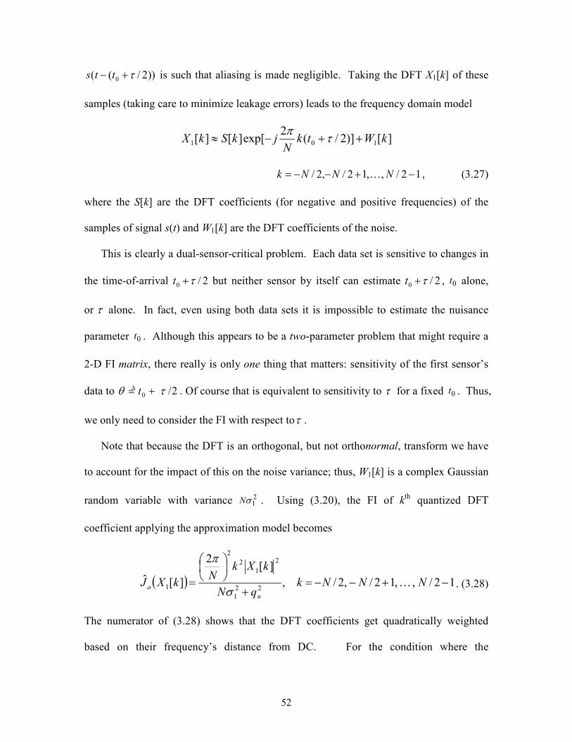
52

))2/(( 0 τ+− tts is such that aliasing is made negligible. Taking the DFT X1[k] of these

samples (taking care to minimize leakage errors) leads to the frequency domain model

][)]2/(2

exp[][][ 101 kWtkN

jkSkX ++−≈ τπ

12/,,12/,2/ −+−−= NNNk K , (3.27)

where the S[k] are the DFT coefficients (for negative and positive frequencies) of the

samples of signal s(t) and W1[k] are the DFT coefficients of the noise.

This is clearly a dual-sensor-critical problem. Each data set is sensitive to changes in

the time-of-arrival 2/0 τ+t but neither sensor by itself can estimate 2/0 τ+t , 0t alone,

or τ alone. In fact, even using both data sets it is impossible to estimate the nuisance

parameter 0t . Although this appears to be a two-parameter problem that might require a

2-D FI matrix, there really is only one thing that matters: sensitivity of the first sensor’s

data to 2/0 τθ +=∆ t . Of course that is equivalent to sensitivity to τ for a fixed 0t . Thus,

we only need to consider the FI with respect toτ .

Note that because the DFT is an orthogonal, but not orthonormal, transform we have

to account for the impact of this on the noise variance; thus, W1[k] is a complex Gaussian

random variable with variance 21σN . Using (3.20), the FI of k

th quantized DFT

coefficient applying the approximation model becomes

( ) 12/,,12/,2/,

][2

][ˆ22

1

2

1

2

2

1 −+−−=+

= NNNkqN

kXkN

kXJn

a Kσ

π

. (3.28)

The numerator of (3.28) shows that the DFT coefficients get quadratically weighted

based on their frequency’s distance from DC. For the condition where the

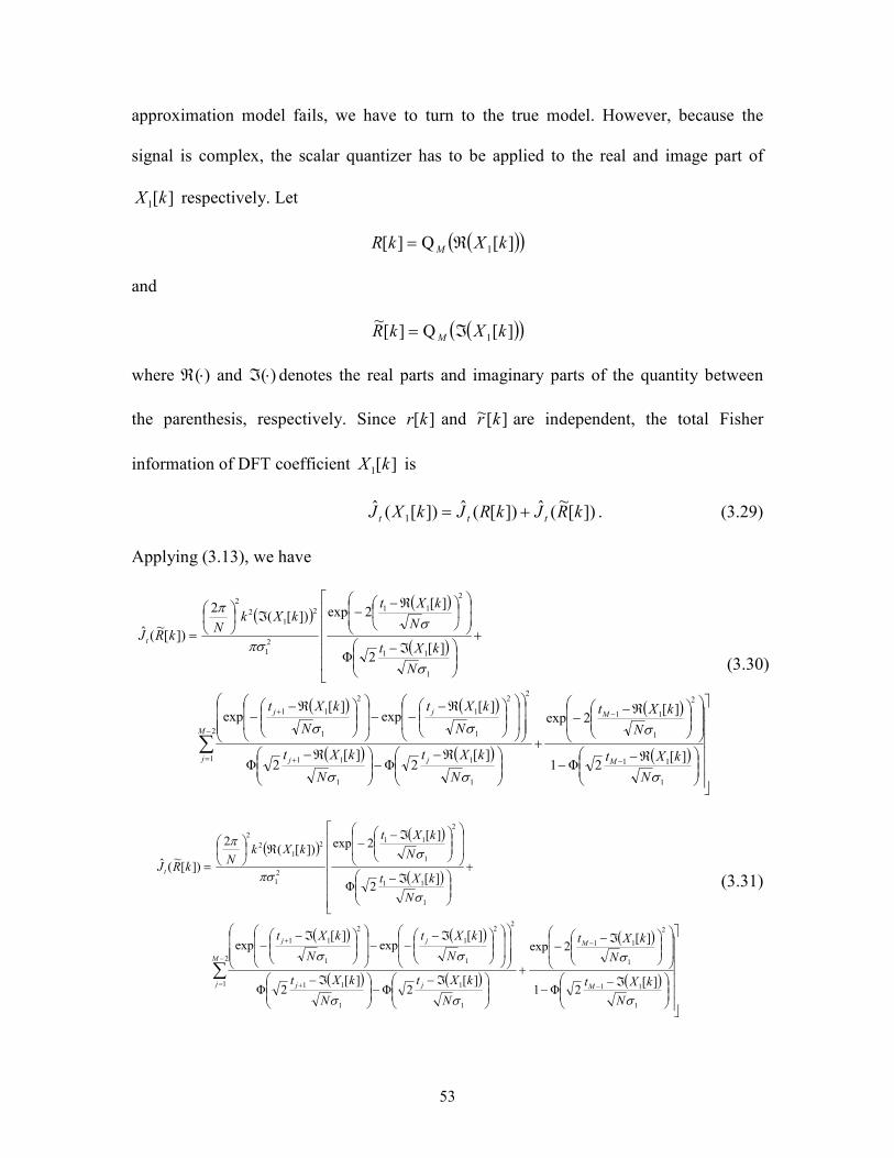
53

approximation model fails, we have to turn to the true model. However, because the

signal is complex, the scalar quantizer has to be applied to the real and image part of

][1 kX respectively. Let

( )( )][Q][ 1 kXkR M ℜ=

and

( )( )][Q][~

1 kXkR M ℑ=

where )(⋅ℜ and )(⋅ℑ denotes the real parts and imaginary parts of the quantity between

the parenthesis, respectively. Since ][kr and ][~ kr are independent, the total Fisher

information of DFT coefficient ][1 kX is

])[~(ˆ])[(ˆ])[(ˆ 1 kRJkRJkXJ ttt += . (3.29)

Applying (3.13), we have

( )( )

( )

( ) ( )

( ) ( )

( )

( )

ℜ−−

ℜ−−

+

ℜ−−

ℜ−

ℜ−−−

ℜ−−

+

ℑ−

ℜ−−ℑ

=

−

−

−

= +

+

∑

1

11

2

1

11

2

1

1

1

1

11

22

1

1

2

1

11

1

11

2

11

2

1

2

1

2

2

][2Φ1

][2exp

][2Φ

][2Φ

][exp

][exp

][2Φ

][2exp])[(

2

])[~(ˆ

σ

σ

σσ

σσ

σ

σ

πσ

π

N

kXt

N

kXt

N

kXt

N

kXt

N

kXt

N

kXt

N

kXt

N

kXtkXk

NkRJ

M

M

M

j jj

jj

t

(3.30)

( )( )

( )

( ) ( )

( ) ( )

( )

( )

ℑ−−

ℑ−−

+

ℑ−−

ℑ−

ℑ−−−

ℑ−−

+

ℑ−

ℑ−−ℜ

=

−

−

−

= +

+

∑

1

11

2

1

11

2

1

1

1

1

11

22

1

1

2

1

11

1

11

2

1

11

2

1

2

1

2

2

][2Φ1

][2exp

][2Φ

][2Φ

][exp

][exp

][2Φ

][2exp

])[(2

])[~(ˆ

σ

σ

σσ

σσ

σ

σ

πσ

π

N

kXt

N

kXt

N

kXt

N

kXt

N

kXt

N

kXt

N

kXt

N

kXtkXk

NkRJ

M

M

M

j jj

jj

t

(3.31)

54

where ( )⋅Φ is the cumulative distribution function for a standard normal PDF and is

defined as

( ) ∫ ∞−−=

x

dttx )2

1exp(

2

1Φ 2

π,

and jt are thresholds that are decided by the chosen scalar quantizer, and range of

both ( )][1 kXℜ and ( )][1 kXℑ .

Using (3.28) to (3.31) in (3.21) with the Lagrange optimization method produces the

results shown in Figure 3.4 to Figure 3.9, which show the performance of our

compression method for a few scenarios. Figure 3.4 and Figure 3.5 show (for

compression ratios (CR) of 4:1 and 8:1, respectively) the TDOA accuracy performance of

our method (labeled “Fisher”) vs. the performance of standard MSE-optimum DFT-based

transform compression (labeled “MSE”) as the SNR1 at sensor S1 is varied; the value of

SNR2 at sensor S2 is fixed at 40 dB. The legend on the plot indicates the cases where just

the signal at S1 is compressed (labeled “S1”) and the cases where the signals at S1 and S2

were both compressed (labeled “S1&S2” and with dashed curves on the plots for easier

identification). For comparison, the performance with no compression is given (labeled

“w/o comp”). The effect of varying SNR2 is shown in Figure 3.6 and Figure 3.7 (for CRs

of 4:1 and 8:1, respectively), where results are shown for the case of both SNR’s

changing but set equal to each other. Figure 3.8 and Figure 3.9 show, for further insight,

the performance of our method and the standard MSE-optimal DFT-based transform

compression relative to the reconstruction error for compression ratios of 4:1 and 8:1,

respectively; the vertical axis shows the norm of the error vector between the original

55

(noisy) signal and its compressed version, which assesses the MSE performance of the

two methods.

In all cases shown, our method provides better TDOA accuracy than the MSE-

optimized method; at moderately high SNR our method is nearly the same as when no

compression is used – even when the CR is 8:1. In some cases the TDOA accuracy of

the MSE-based method is quite poor (especially at higher CRs and when both signals are

compressed) – indicating that optimizing MSE provides no guarantee of good

performance relative to parameter estimation accuracy. Also note that when both sensor’s

signals have been compressed at 8:1, our method’s performance is degraded a small

amount where as the performance of the MSE-based method is severely degraded.

However, notice in Figure 3.8 and Figure 3.9 that the TDOA-optimized compression

performs very poorly from the reconstruction point of view – this shows that compression

for reconstruction and compression for TDOA accuracy are in conflict with each other;

our method favors TDOA accuracy at the expense of MSE while the reference method

favors MSE at the expense of TDOA accuracy.

The above algorithm can be also extended to apply to image recognition applications.

The task in image recognition is finding a specific match in an image. However this

image may be distorted and compressed from the original. The Fisher-information-based

algorithms that aim to maximize the ability of images to recognize are detailed in

Appendix C.

3.1.4.2 Compression for FDOA Estimation

It is possible to locate a signal source by first estimating the FDOA between several

pairs of sensors and then using the FDOA estimates to estimate the source location [66].

56

10 15 20 25 30 35 400

5

10

15

20

25

30

35

40

45

50TDOA Performance SNR

2=40 dB CR=4:1

SNR1 (dB)

RMS TDOA Error (ns)

w/o compMSE (S1)MSE (S1&S2)Fisher (S1)Fisher (S1&S2)

Figure 3.4: TDOA accuracy vs SNR of pre-compressed sensor S1 signal for a CR of 4:1; the SNR of the

sensor S2 signal was 40 dB.

10 15 20 25 30 35 400

20

40

60

80

100

120


2 = 40 dB CR=8:1

SNR1 (dB)

RMS TDOA Error (ns) w/o comp

MSE (S1)MSE (S1&S2)Fisher (S1)Fisher (S1&S2)



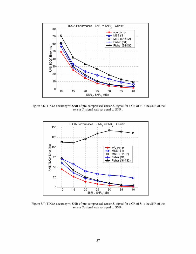
57

10 15 20 25 30 35 400

10

20

30

40

50

60

70


1 = SNR

2 CR=4:1

SNR1, SNR

2 (dB)

RMS TDOA Error (ns)



sensor S2 signal was set equal to SNR1.

10 15 20 25 30 35 400

25

50

75

100

125


1 = SNR

2 CR=8:1

SNR1, SNR

2 (dB)

RMS TDOA Error (ns)

w/o comp MSE (S1) MSE (S1&S2) Fisher (S1) Fisher (S1&S2)


sensor S2 signal was set equal to SNR1.

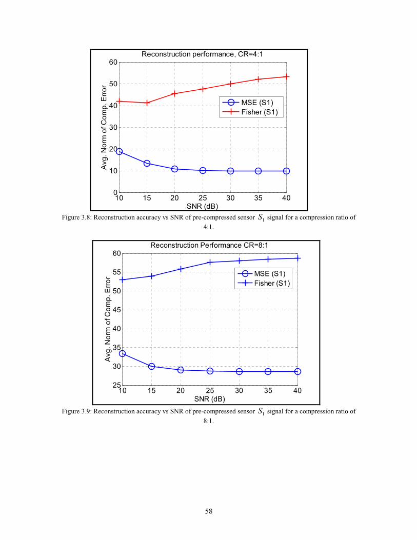
58

10 15 20 25 30 35 400

10

20

30

40

50

60

SNR (dB)

Avg. Norm of Comp. Error

Reconstruction performance, CR=4:1

MSE (S1)

Fisher (S1)

Figure 3.8: Reconstruction accuracy vs SNR of pre-compressed sensor 1S signal for a compression ratio of

4:1.

10 15 20 25 30 35 4025

30

35

40

45

50

55

60Reconstruction Performance CR=8:1

SNR (dB)

Avg. Norm of Comp. Error MSE (S1)

Fisher (S1)

Figure 3.9: Reconstruction accuracy vs SNR of pre-compressed sensor 1S signal for a compression ratio of

8:1.

59

It is well known (see, e.g.,[67],[68]) that for FDOA estimation, the Cramer-Rao bound is

inversely proportional to the so-called RMS duration Drms of the signal , which is defined

by

∫

∫∞

∞−

∞

∞−=dtts

dttstDrms

2

22

)(

)(

. (3.32)

Because the Fisher information is the reciprocal of the Cramer-Rao bound, the Fisher

information for FDOA estimation is directly proportional to Drms. This analysis of the

Fisher information for FDOA estimation explicitly drives the choice of the identity

transform (which is an ON transform) to provide the ability to discard time components

that contribute little to the Fisher information. Thus we will directly quantize the

complex-valued signal samples, using individual quantizers for the real and imaginary

parts.

Given this insight, we now derive the form for the signal sensitivity function )(⋅Γ in

terms of the samples of the received signal. The signal model for two passively-received

signals having an unknown FDOA of v is given by

2/,,12/,2/][][][

2/,,12/,2/][][][

2

)2/(

2

1

)2/(

1

0

0

NNNnnwensnx

NNNnnwensnx

nvj

nvj

K

K

+−−=+=

+−−=+=−

+

ν

ν

, (3.33)

where v0 is an unknown nuisance parameter that can not be estimated, and wi[n] is

complex Gaussian noise with variance of 2iσ , with 2

1σ assumed known. The discussion in

Appendix D addresses why symmetric indexing is chosen in (3.33). The model in (3.33)

is mathematically identical to the TDOA model for the DFT transform in (3.27) and

therefore we can use the previous results to immediately state that the FI of quantized

per-sample in terms of approximation model becomes

60

( ) 2/,,12/,2/,][

2

1][ˆ

22

1

2

1

2

1 NNNnq

nxnnxJ

n

a K+−−=+

=σ

. (3.34)

On the other hand, in terms of calculation of ( )][ˆ1 nxJ t by applying (3.13), we let

( )( )][Q][ 1 nxnr M ℜ= and ( )( )][Q][~ 1 nxnr M ℑ= , due to the reason that ][nr and ][~ nr are

independent, the total Fisher information of quantized samples ][ˆ1 nx is

])[~(ˆ])[(ˆ])[ˆ(ˆ 1 nrJnrJnxJ ttt += . (3.35)

where

( )( )

( )

( ) ( )

( ) ( )

( )

( )

ℜ−−

ℜ−−

+

ℜ−−

ℜ−

ℜ−−−

ℜ−−

+

ℜ−

ℜ−−

ℑ=

−

−

−

= +

+

∑

1

11

2

1

11

2

1

1

1

1

11

22

1

1

2

1

11

1

11

2

1

11

2

1

2

1

2

][2Φ1

][2exp

][2Φ

][2Φ

][exp

][exp

][2Φ

][2exp

4

])[(])[(ˆ

σ

σ

σσ

σσ

σ

σ

πσ

nxt

nxt

nxtnxt

nxtnxt

nxt

nxt

nxnnrJ

M

M

M

j jj

jj

(3.36)

( )( )

( )

( ) ( )

( ) ( )

( )

( )

ℑ−−

ℑ−−

+

ℑ−−

ℑ−

ℑ−−−

ℑ−−

+

ℑ−

ℑ−−

ℜ=

−

−

−

= +

+

∑

1

11

2

1

11

2

1

1

1

1

11

22

1

1

2

1

11

1

11

2

1

11

2

1

2

1

2

][2Φ1

][2exp

][2Φ

][2Φ

]][exp

][exp

][2Φ

][2exp

4

])[(])[~(ˆ

σ

σ

σσ

σσ

σ

σ

πσ

nxt

nxt

nxtnxt

nxtnxt

nxt

nxt

nxnnrJ

M

M

M

j jj

jj

(3.37)

where the definitions of )Φ(⋅ and jt are same as in (3.30) and (3.31).

Using these results (3.34)-(3.37) in (3.21) with the Lagrange optimization method

produces the results shown in Figure 3.10 and Figure 3.11, which show the performance

of our method (labeled “Fisher”) and the standard MSE-optimum time-domain

61

10 15 20 25 30 35 400

2

4

6

8

10

12

14

16

FDOA Performance SNR2 = 40 dB CR=4:1

SNR1 (dB)

RMS FDOA Error (mHz)

w/o comp MSE (S1) MSE (S1&S2) Fisher (S1) Fisher (S1&S2)

Figure 3.10: FDOA accuracy vs SNR of pre-compressed sensor S1 signal for a CR of 4:1; the SNR of the


10 15 20 25 30 35 400

5

10

15

20

25

30

35

TDOA Performance SNR2 = 40 dB CR=8:1

SNR1 (dB)

RMS FDOA Error (mHz)


Figure 3.11: FDOA accuracy vs SNR of pre-compressed sensor S1 signal for a CR of 8:1; the SNR of the


62

compression (labeled “MSE”) relative to the FDOA RMS error value for compression

ratios of 4:1 and 8:1 as SNR1 at sensor 1S is varied; the value of SNR2 at sensor 2S is

fixed at 40 dB, respectively; We have included the case where just the signal at 1S is

compressed (labeled “S1”) as well as the case where the signals at 1S and 2S were both

compressed (labeled “S1&S2”); these figures also show the FDOA RMS error that is

achieved when no compression is used (labeled “w/o compression”). In all cases shown

in Figure 3.10 and Figure 3.11, our method provides better FDOA accuracy than the

MSE-optimized method.

3.1.4.3 Compression for DOA estimation

Direction of arrival (DOA) estimation is a classical problem that has been

extensively studied from numerous aspects. A wide variety of techniques have been

proposed for the DOA estimation of narrowband sources in the far-field [4],[70], [71].

Let us consider an array of M uniformly spaced omni-directional sensors arranged in a

uniform linear array (ULA). Let d denote the spacing between two consecutive sensors.

Let λ denote the signal’s wavelength, and let )9090( 00 <<− ϕϕ denote DOA of a

narrowband signal that is illuminating the array.

The DOA is measured clockwise with respect to the normal to the line of sensors,

then the matrix of observations (snapshots) is given by

Nittst iii ,,2,1),()()()( K=+= wαx ϕ , (3.38)

where received signal vector [ ]TiMii txtxt )(,),()( 1 L=x and receive noise vector

[ ]TiMii twtwt )(,),()( 1 L=w and the steering vector is given by

[ ]TwMjjw ss ee)1(

,,,1)(−−−= Lϕα (3.39)

63

where the spatial frequency sw is given by

λ

ϕππ

sin22

dfw ss == .

Let us look at a two-sensor array ( 1S and 2S ) to be consistent with the context in this

Chapter. Despite being of interest in itself, the two-sensor array case also gives us a

glimpse at the effects quantization has on multi-sensor array. Let the snapshot at the two

sensor ( 1S and 2S ) be

1,,1,0][)]2/(exp[][][

1,,1,0][)]2/(exp[][][

202

101

−=++−=

−=+−−=

Nmmwwwjmsmx

Nmmwwwjmsmx

s

s

K

K. (3.40)

After we stack all the received samples ][1 mx into a vector )(1 swx and then we perform

any ON transform on )(1 swx to get )(1 swχ whose elements are ][1 mχ .

1,,1,0][)]2/(exp[][][ 1011 −=+−−= Nmmwwjmm s Kωξχ (3.41)

It should be noted that the best ON transform is the phase-invariant transform, otherwise,

(3.40) does not hold. The Fisher information with respect to the unknown parameter sw

according to (3.18) is computed by

∑=

=N

m

ww mJss

1

2

12

1

)(2

1ξ

σ, (3.42)

where

== −

d

wdw s

s πλ

ϕλ

ϕπ2

sin,sin2 1 . Then the Fisher information with respect to

DOA ϕ is computed by [4]

=

∂

∂= ∑

=

N

m

ww

s

s md

Jw

wJ

ss

1

2

12

1

22

)(2

1

cos2

)(ξ

σϕπλϕ

ϕ . (3.43)

64

Observing (3.43), it is clear to see that the Fisher information of DOA ϕ can be

decomposed into the product of two independent terms, one is a function of DOA ϕ and

distance between the sensors d and the signal’s wavelength λ and the other completely

depends on the data )(1 mξ and variance of noise 2

1σ . Clearly this problem can be

handled by applying our “maximize Fisher information” approach only to the part of the

Fisher information that is within the square brackets in (3.43).

Proceeding as before, in terms of the partial Fisher information we intend to

maximize, according to (3.20),

22

1

2)(

2

1)(ˆ

m

maq

mJ

+=

σ

χχ , (3.44)

and

( )( )

( )

( ) ( )

( ) ( )

( )

( )

ℜ−−

ℜ−−

+

ℜ−−

ℜ−

ℜ−−−

ℜ−−

+

ℜ−

ℜ−−

ℑ=

−

−

−

= +

+

∑

1

1

2

1

1

2

1

11

1

22

1

2

1

1

1

1

2

1

1

2

1

2

2Φ1

2exp

2Φ2Φ

expexp

2Φ

2exp

4

)(])[(ˆ

σχ

σχ

σ

χ

σ

χ

σ

χ

σ

χ

σχ

σχ

πσ

χ

mM

mM

M

j mjmj

mjmj

m

m

m

t

t

t

tt

tt

t

t

mrJ

(3.45)

( )( )

( )

( ) ( )

( ) ( )

( )

( )

ℑ−−

ℑ−−

+

ℑ−−

ℑ−

ℑ−−−

ℑ−−

+

+

ℑ−

ℑ−−

ℜ=

−

−

−

= +

+

∑

1

1

2

1

1

2

1

11

1

22

1

2

1

1

1

1

2

1

1

2

1

2

2Φ1

2exp

2Φ2Φ

expexp

)(2Φ

2exp

4

)(])[~(ˆ

σχ

σχ

σ

χ

σ

χ

σ

χ

σ

χ

σχ

σχ

πσ

χ

mM

mM

M

j mjmj

mjmj

sm

m

m

t

t

tt

tt

wt

t

mrJ

(3.46)

65

Using these results (3.44)-(3.46) in (3.21) with the Lagrange optimization method

produces the results shown in Figure 3.12 and Figure 3.13, which show the performance

of our method (labeled “Fisher”) and the standard MSE-optimum time-domain

compression (labeled “MSE”) relative to the DOA RMS error value for compression

ratios of 4:1 and 8:1 as SNR1 at sensor 1S is equal to SNR2 at sensor 2S and is varied from

10 dB to 40 dB; The wavelet ON transform (Coif5 wavelet, see [72] ) is used. Regarding

the parameter in (3,42), we choose the distance between the two sensors are equal to the

wavelength, λ=d , and the true DOA 0=ϕ which corresponds to the direction that has

the better worse than other angles (See our discussion on the minimax problem). In all

cases shown in Figure 3.12 and Figure 3.13, our method provides better DOA accuracy

than the MSE-optimized method. The main reason why MSE is inferior to maximizing

SNR is in that MSE pays equal weight to all the coefficients, even the coefficients of

small amplitude are severely corrupted by the noise whereas maximizing SNR give more

bits to those coefficients whose magnitude is much higher than the noise lever. In this

case, maximizing SNR has partial denoising functionality.

3.1.4.4 Compression for Signal Estimation

As a further illustrative (though perhaps not entirely practical) example of the

flexibility of our Fisher-information-driven viewpoint we consider the scenario

1,,1,0][][][

1,,1,0][][][

22

101

−=+=

−=+−=

Nnnwnsnx

Nnnwnnsnx

K

K

(3.47)

where the goal is to compress the data x1[n] at sensor S1 and send it to sensor S2 where it

would be used together with the S2-local data x2[n] to estimate the underlying signal s[n].

For simplicity here we assume that the relative delay n0 is known either from previous

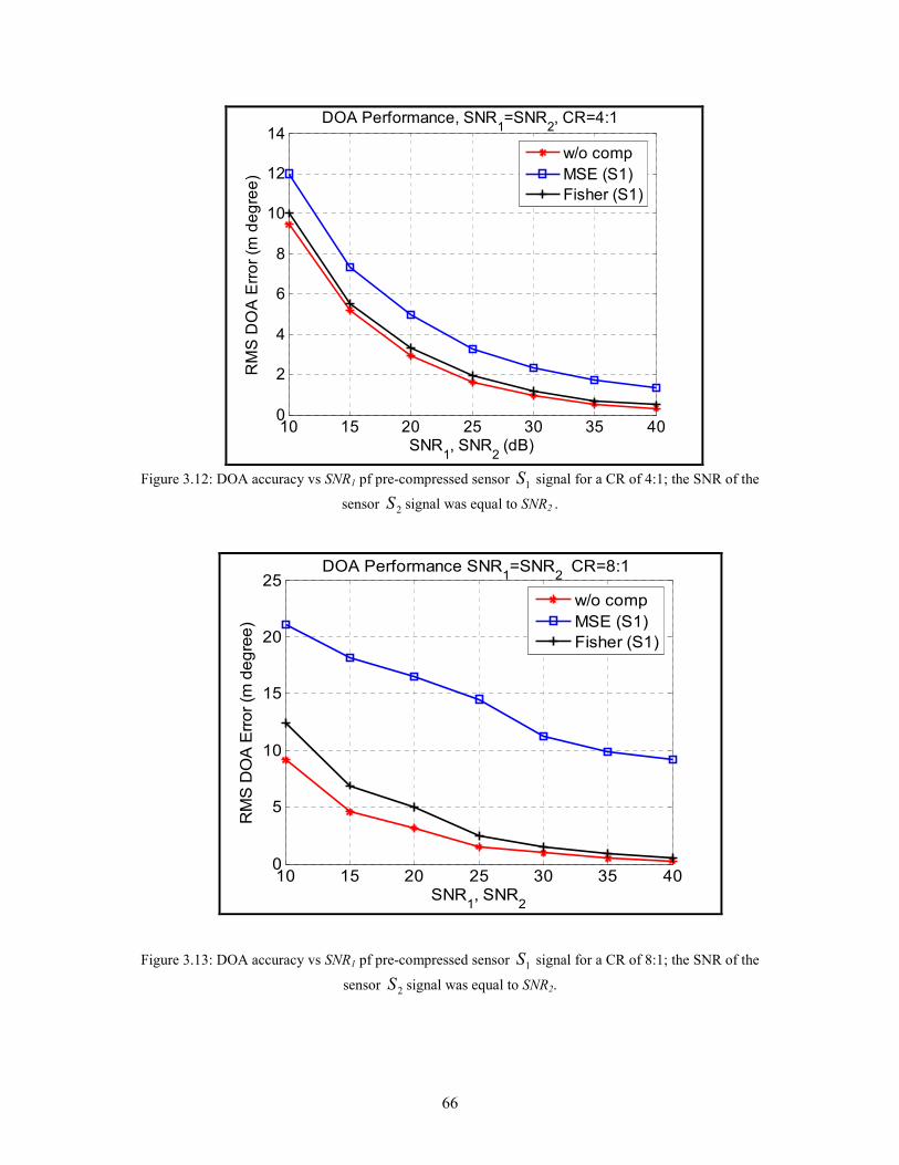
66

10 15 20 25 30 35 400

2

4

6

8

10

12

14

SNR1, SNR

2 (dB)

RMS DOA Error (m degree)

DOA Performance, SNR1=SNR

2, CR=4:1

w/o comp

MSE (S1)

Fisher (S1)

Figure 3.12: DOA accuracy vs SNR1 pf pre-compressed sensor 1S signal for a CR of 4:1; the SNR of the

sensor 2S signal was equal to SNR2 .

10 15 20 25 30 35 400

5

10

15

20

25

SNR1, SNR

2

RMS DOA Error (m degree)

DOA Performance SNR1=SNR

2 CR=8:1

w/o comp

MSE (S1)

Fisher (S1)

Figure 3.13: DOA accuracy vs SNR1 pf pre-compressed sensor 1S signal for a CR of 8:1; the SNR of the

sensor 2S signal was equal to SNR2.

67

estimation processing or from some other a priori knowledge (and this is where we veer

from a practical example into an illustrative one).

We can estimate the DFT of s[n] instead of estimating s[n] directly, so after taking the

DFT of x1[n] and x2[n], we have

1,,1,0][][][

1,,1,0][]2exp[][][

22

101

−=+=

−=+−=

NmmWmSmX

NmmWmnjmSmX

K

Kπ (3.48)

From this we see that X1[m] and X1[m] satisfy the complex classical linear model [4] so

(3.48) is equivalent to

1

0

0

0

1

)]1(2exp[00

0]2exp[0

00]02exp[

WSX +

−−

−

−

=

Nnj

nj

nj

π

π

π

L

MOMM

L

L

(3.49)

and

.

100

010

001

2 2WSX +

=

L

MOMM

L

L

(3.50)

Applying results for the Fisher information for the classical linear model from [4] to

(3.48) and (3.49) gives

2

2

2

1

21

11),(

σσ NNJ +=XX (3.51)

From this, let us assume fine quantization on 1X , that is when the approximation model is

valid, we see that after quantization the per-coefficient Fisher information to use in (3.20)

for optimizing the compression of sensor S1’s data becomes

68

1,,1,0,1~

221

−=+

= NnqN

J

n

n Kσ

. (3.52)

However, maximizing this is equivalent to minimizing MSE. Thus, this is an illustration

that our method is flexible enough to cover the two cases mentioned in Section 3.1.1:

parameter estimation and signal estimation. Also, it shows that when MSE is appropriate

our method inherently uses it.

In practice, sensor networks may also be tasked with multiple estimation tasks from

multiple users, this would make it a multiple parameter problem where the compression

requirements are in conflict with each other. This is discussed in Chapter 4.

3.2 Chernoff-Distance-Based Data Compression for Detection

3.2.1 Overview of Previous Work

Using the same set-up as in Section 3.1, we can formulate target detection based on

compressed data 1x from 1S and local data 2x at 2S as a statistical hypothesis testing

problem:

τ

0

1

),ˆ(

),ˆ(),ˆ(

210

21121

H

H

p

pL

<

>=

xx

xxxx , (3.53)

where ),ˆ( 210 xxp and ),ˆ( 210 xxp are joint PDF of 1x and 2x , and the threshold τ in

the LRT (3.53) can be chosen to minimize the probability of error eP or the probability of

miss ( missP ). Unfortunately, both eP and missP are notoriously intractable functions of the

N-variate distributions 0p and 1p [73], and in general, can only be evaluated

experimentally. Hence, it is not feasible to optimize the parameters of complex systems

such as lossy coders with respect to eP or missP . Some alternative performance measure

69

must be used instead to provide the tractable metric to quantify the degradation of

compression on detection accuracy.

In comparison with the few discussions of compression for estimation in literature,

various optimality criteria have been analyzed for the problem of optimal quantization for

hypothesis testing. Most focus on restricting the encoder to being a scalar quantizer. The

composite hypotheses 0=θ versus 0>θ was considered in [42] and the efficacy of the

sufficient statistic was used as the objective function. Asymptotically optimal

companding functions for scalar quantizers were then derived. In [38] [43], a generalized

“f-divergence”, of the which the Kuallback-leibler distance is a special case, was used as

an optimality criterion and its asymptotic quantization effects are studied. A deflection

criterion similar to signal-to-noise ratio (SNR) under one of two simple hypotheses is

considered in [44], where it is found that maximization of this deflection criterion is by

quantizing the likelihood ratio rather then the observation itself. Some properties of these

so-called likelihood ratio quantizers are further explored in [45], and their optimality with

respect to statistical divergence are also investigated. A method of combining vector

quantization and classification was developed in [46][47] by defining an objective

function that incorporates MSE and Bayes risk. [48] uses Ali-Silvey distances as

optimality criteria and investigate non-asymptotic quantizer effects. The use of alpha

entropy as an optimality criterion was proposed in [49] because it gives the exponential

decay to zero of the total probability of error of a binary hypothesis test with equal priors,

according to a theorem of Chernoff. The distributed hypothesis testing problem with

quantized observations is directly addressed in [50]. Optimal scalar quantizers are derived

with the Bhattacharyya distance as the objective function and an iterative design

70

algorithm is developed. The Chernoff distance and Kullback-Leibler distance are used to

set the information-theoretic bounds on target recognition performance based on

degraded image data [51] [52].

The success of designing compression for estimation based on Fisher information

motivates us to investigate performance measures that provide tight bounds on eP and

missP . Since the ability to distinguish between two statistical hypotheses depends on the

respective data distributions, using measures of distance or dissimilarity between two

distributions sounds natural and is promising.

Ali and Silvey studied a generic category of distances that measure the dissimilarity

between two distribution [48]. The Ali-Silvey class of distances is based on an axiomatic

definition and takes the general form:

( ) ))((01,0 LCEfppd = , (3.54)

where f is any increasing function, C is any convex function on ),0[ ∞ , 01 / ppL = is the

likelihood ratio for the data, and 0E is the expectation under hypothesis 0H . It is

convenient to also allow pairs ),( Cf , where f is decreasing and C is concave.

The Ali-Silvey class of distances is decreased under application of many-to-one

maps such as quantization. For our problem at hand, it means

( ) ( ))(),(),ˆ(),ˆ( 1010 xxxx ppdppd ≤ , (3.55)

where x and x are some 1×N compressed data vector and unquantized data vector.

Although it has been showed in [43] and [48] how Ali-Silvey distance can be used

for optimal quantizer design in detection problems, they limited their design to scalar

quantizers. Besides the decrease of distance under quantization, the other attractive

71

property of the Ali-Silvey distance is that they are invariant under application of

invertible maps to the data, which directly makes the powerful transform-based

compression coding possible.

Chernoff distance (2.23) is in the Ali-Silvey class. More specifically,

)]([ln

)(

)()(ln)(

0

0

1

0

x

x

xx

s

s

LE

dxp

pps

−=

−= ∫µ

, 10 << s (3.56)

where )ln()( ⋅−=⋅f is convex increasing and 10,)( <<⋅= sC s is concave. Chernoff

distance is the key factor for the Chernoff upper bound of probability of error eP . [51]

provides several bounds derived from Ali-Silvey distance, including Chernoff bound and

uses these bounds to guide the design of a quantizer. It is natural to suspect the design

that reduces only an upper bound criterion may not always reduce the probability of error.

However, Chernoff bound is different from other bounds in that Chernoff’s theorem [57]

clearly exhibits the exponential tightness of the Chernoff bound given that the samples

that make up x are I.I.D. Exponential tightness means that for large N .

)])((exp[)])((exp[ εµεµ +−<<−− sNPsN e , (3.57)

where )(sµ is the Chernoff distance for each sample. Clearly any design which

increase )(sµ must (eventually for large N ) reduce the probability of error.

Clearly, compression of the data vector x using a lossy algorithm changes the

underlying PDF to that of the post-compression data x available for detection, and

therefore decreases the magnitude of the Chernoff distance. Similarly, our goal here is to

seek operational rate-distortion methods to maximize the magnitude of the Chernoff

72

distance represented by the data set x while satisfying a budget R on the rate used to

represent the data set.

Let )(xsµ and )ˆ(xsµ be the Chernoff distance of the original data x and the

compressed data x , respectively. The optimal approach is to compress to R bits such

that we satisfy

[ ])ˆ()(minˆ

xxx

ss µµ − , (3.58)

where the minimization is over all compressed x that meet the bit budget R. This is

equivalent to maximizing the post-compression )ˆ(xsµ .

3.2.2 Compressing to Maximize Chernoff Distance

Let noisy measurement xk collected at sensor node Sk (k = 1, 2) be modeled as

2,1, =

+=

=k

kk

kk

wsx

wx, (3.59)

where s is an unknown deterministic signal vector and wk is a noise vector with w1 and

w2 independent of each other. Measurement vector x1 will be compressed at S1 and sent

to S2; the decompressed vector 1x is then used with x2 to decide the presence of s . By

independence (See Appendix A), )()ˆ(),ˆ( 2121 xxxx sss µµµ += , so we need only maximize

)ˆ( 1xsµ .

Similar to the goals in Section 3.1, but expressed here with the Chernoff distance, the

general goal of our transform-coding compression method is as follows: we use an

orthonormal (ON) basis Nnn 1 =φ with nχ as the coefficients for x1, and ON expansion

conserves Chernoff distance, hence )()( 1xsns µχµ = . Only those nχ with significant

73

contribution to the Chernoff distance should be selected and quantized. Let

,,2,1 NK⊂Ω be the set of indices of a selected set of coefficients; let | Ω∈= nbB n be

a set of bit allocations to the selected coefficients; let |ˆ Ω∈nnχ be the selected

coefficients after quantization using the allocation set | Ω∈= nbB n . The resulting

compressed signal is then given by

∑Ω∈

=n

nnφx χˆ1 .

Our goal, then, is to find a selection set Ω and a bit allocation | Ω∈= nbB n that solves

)ˆ(max 1,

xsBµ

Ω subject to Rb

n

n ≤∑Ω∈

(3.60)

Let ( )nbnr χQ= and the PMF of nr under different hypotheses iH , 1,0=i can be

calculated as

∫∫

+

==

==

1

)()(

];[)|ˆProb(ˆ

][

j

j

j

j

t

tnni

I

nni

in

x

nrijn

dpdp

HbfHxr

χχχχ , (3.61)

The total Chernoff distance of the independent discrete quantized coefficient nr can be

computed by

( ) ( )∑ ∑−

=

−

−=

1

0

1

ˆ1

0

ˆ];[];[ln)(

N

k j

s

n

x

r

s

n

x

rns HbfHbfr j

n

j

nµ (3.62)

See appendix B, the close form of Chernoff distances with respect to each nr is

( ) ( )[( ) ( )( ) ( ) ( )( )

( )( ) ( )( ) ]snM

s

M

M

j

s

njnj

s

jj

s

n

s

n

r

st

tt

tttt

ttn

ξηη

ξηξηηη

ξηηχµ

−−−+

+−−−×−+

+−=

−−

−

−

=+

−+

−

∑

1

1

1

2

1

1

1

1

1

1

1,

11

ln)(

(3.63)

74

where nξ is the ON transform of noise-free signal ][ns and )(⋅η is the cumulative

distribution function for PDF of ON transformed noise vector 1w .

If we do not insist on the optimum selection of the Chernoff parameter s , we may

obtain another distance, called the Bhattacharyya distance which also gives us the upper

bound

)]([ln)( 2/1

02/1 xx LE−==µ . (3.64)

We prefer using the Bhattacharyya distance rather than the Chernoff because the

Bhattacharyya distance is a popular, simple measure of similarity between two

distributions or convenient measure of class separability, if the number of classes is two.

Furthermore, it gives an upper bound of the Bayes error [2] if the distributions are normal.

Other divergence measures in the literature are not as closely related to Bayes errors as is

the Bhattacharyya bound. However, all discussions about the Bhattacharya distance in

this dissertation could be extended to the Chernoff.

If the noise 1w at 1S is zero-mean, white Gaussian noise, Bhattacharyya distance

takes a simple form like

2

1

12/18

1)(

σµ

ssx

H

= . (3.65)

After ON transformation, and applying the approximation model that we used in Section

3.1 jointly, the post-compression Bhattacharyya distance becomes

22

1

2

2/1,8

1)(

n

n

naq+

=σ

ξχµ . (3.66)

It is obvious that maximizing (3.66) in terms of compression is equivalent to maximizing

the Signal-to-Noise-and-Quantization ratio. This suits for the compression under the

75

assumption that the signal is deterministic. The goal for compression for detection will be

to keep the signal level above the noise and quantization noise floor as far as possible.

Notice that (3.66) is only for Gaussian noise, the expression for Bhattacharyya distance

under other distribution of noise will be different from (3.66).

If we use the noisy quantities nχ rather than the noise-free values nξ , the

operational Bhattacharyya-distance-based distortion function we use to assess the nth

coefficient quantized to bn bits is

≥

<≤

=

=

)( if),ˆ(ˆ

)(1 if),ˆ(ˆ

0 if,0

)ˆ(ˆ

2/1,

2/1,2/1

σγχµ

σγχµχµ

nnt

nna

n

n

b

b

b

, (3.67)

and we seek a bit allocation set ,,2,1|0 NnbB n K∈≥= that solves

RbN

n

n

N

n

nB

≤

∑∑

== 11

2/1 osubject t)ˆ(ˆmax χµ . (3.68)

Simulation results are skipped because maximizing signal SNR for detection is well

known and a metric very similar to (3.66) has been applied before in [51][52], although

they do not provide the rigid operational function (3.67) as we do. The real interest here

is to complete the inference-centric compression framework and explore how multiple

measures (for multiple inferences) drive the specification of new multiresolutional

characteristic of the data needed to support multiple sequential and simultaneous

inferences.

76

CHAPTER 4

Data Compression for Simultaneous Tasks of Multiple Inference Quantities

In Chapter 3, we have considered data compression for single estimation/detection

tasks. However, as pointed out elsewhere [27], sensor networks may also be tasked with

multiple inference tasks from multiple users. For example, sensor 2S may use the shared

compressed data stream from sensor 1S to simultaneously accomplish joint TDOA and

FDOA measurements. However, compression for TDOA (3.27)-(3.30) and compression

for FDOA (3.33)-(3.36) conflict such that compression for TDOA favors the frequency-

domain coefficients of high frequencies whereas compression for FDOA favors the time-

domain coefficients of early or late times. For such simultaneous estimation tasks, it is

crucial to find the right way to balance the conflicts of compression for different

parameters. On the other hand, sensor 1S may send data for sensor 2S , where detection is

first performed to check if both sensors have the signals intercepted from the same

emitter, and then once detected, joint TDOA/FDOA will be performed to locate the

emitter. So we also need to find ways to balance the conflicting compression

requirements between detection and estimation. To solve this problem, in this Chapter,

we will derive multiple distortion measures to assess the information utility of data

subsets for the multiples inferences and develop the corresponding numerical

optimization methods to achieve desired trade-offs based on the information utility.

77

4.1 Data Compression for Simultaneous Multiple Parameter

Estimation without Detection

Different from single parameter estimation, now we have a parameter vector

],,[ 1 pθθ K=θ sought to be estimated, intuitively, we will say that the compression

algorithm 1ε is distinct from the compression 2ε if at least one of the estimated value jθ

by 1ε is distinct from the corresponding variable by 2ε . To design the optimal

compression, we need to have criteria for comparing compression algorithms. As

suggested in Chapter 2, the natural and ultimate choice of criteria to compare different

algorithm relies on their error covariance matrix which is lower bounded by and can be

quantified by the Cramer-Rao Lower Bound matrix (2.7). Therefore, we can claim that

compression algorithm 1ε is considered as preferable to compression algorithm

2ε ( 21 εε > ) if the difference of ),(CRB),(CRB 12 εε xx − is a positive matrix. However, it

is not obvious how to use the matrix ),(CRB kεx as a distortion measure because

compression algorithms often require a scalar measure for efficiency. The open question

for us is how we map ),(CRB kεx into a scalar measure of information utility which

exploits the information content that is carried by ),(CRB kεx and is proportional to the

“size” of the high probability uncertainty region of the estimate ofθ as well.

The determinant ( )),(CRBdet kεx is proportional to the volume of the rectangular

region enclosing the core ellipsoid of covariance ellipsoid of any estimate. Hence, the

first information utility function we choose is ( )),(CRBdet kεx . Although the volume of

the high probability regions seems to be a useful measure, there are cases in which this

measure underestimates the residual uncertainty. In case the smallest principal axis

78

shrinks to zero, the volume of the uncertainty ellipsoid is zero, while the uncertainties

along the remaining principal axes might remain large. An alternative measure that

avoids this shortcoming of ( )),(CRBdet kεx would be ( )),(CRBtr kεx , which is

proportional to the circumference of the rectangular region enclosing the covariance

ellipsoid. Therefore, the distortion measure for multiple parameter estimation must be

able to minimize ( )),(CRBdet kεx and ( )),(CRBtr kεx under the bit constraints.

However, we found that deriving closed-form distortion measures based on either

( )),(CRBdet kεx or ( )),(CRBtr kεx is difficult - even for a single parameter case, such as

TDOA-only case [24],[60]. Therefore, with the desire to design the most efficient

compression algorithms, we resort again to Fisher information.

In Chapter 3, we have used Fisher information to derive transform-coding schemes

for the signal parameter cases where the Fisher information (FI) is a scalar. However,

when multiple parameter parameters are to be estimated the FI becomes the Fisher

information matrix (FIM). The Cramer-Rao bound (2.7) states that the error covariance

Σ of any unbiased estimator of x satisfies

),(CRB),(1 kk εε xxJ =≥Σ − . (4.1)

It can be shown that the Fisher information matrix (FIM) is related to the surface area of

a high probability region, which is a notion of the “size” of the region [1]. It is natural to

assume that maximizing the size of the FIM is equivalent to minimization of the size of

the CRB. Similar to the measures for CRB, possible forms of the information utility

function using the FIM are ( )),(det kεxJ and ( )),(tr kεxJ .

79

Besides easier manipulation of J rather then CRB, ( )),(det kεxJ and

( )),(CRBdet kεx or ( )),(tr kεxJ and ( )),(CRBtr kεx can be verified as equivalent to each

other due to the close relationships between J and CRB in (4.1). First of all, it is easy to

show from matrix theory that minimizing ( )),(CRBdet kεx is equivalent to

maximizing ( )),(det kεxJ . Second, the following relationship between ),(CRB kεx and

),(1 kεxJ− provides the justification that the maximization of ( )),(tr kεxJ is equivalent to

the minimization of ( )),(CRBtr kεx .

Because J is positive definite, 1CRB −= J is positive definite, too. Let the

eigenvalues of J be λi >0 (i=1,…,n), then ∑=

=n

i

i

1

tr λ(J) and ∑=

− =n

i

i

1

1 /1tr λ)(J . Using

the Cauchy-Schwarz inequality gives

[ ] )tr(J)tr(J 1−

==

=≤

= ∑∑k

i

i

k

i

i

n

i

nin

11

/1

1

1

, λλ

λ

λλλ MK

, (4.2)

That is, )/tr(tr 21 J)(J n≥− . Thus the maximization of (J)tr tends to bring the minimization

of )(J 1tr − , providing further justification for the choice of the trace. Hence, in the sequel,

we will use ( )),(det kεxJ or ( )),(tr kεxJ instead of ( )),(CRBdet kεx or ( )),(CRBtr kεx to

derive the theory and algorithm for compression for simultaneous parameter estimation.

Suppose we have two sensor nodes that intercept a common signal and wish to share

data to estimate a parameter vector θθθθ. At sensor node Sk we model the received signal

vector xk as

2,1,)( =+= kkkk wθsx , (4.3)

80

where )(θsk is an unknown deterministic vector dependent on the unknown

deterministic parameter vector θθθθ, and wk is an additive noise vector with w1 and w2

independent. To simplify the discussion, but without loss of generality, we will assume

w1 is a zero-mean, Gaussian noise vector whose covariance matrix Σ is known or

estimated. The extension to other noise distributions is obvious because the following

procedure for Gaussian noise is quite general (see Chapter 3, the comprehensive study of

other noise distribution will be left for further work). Second, we will focus on the two

parameter case. Here we use an orthonormal (ON) transform for the linear invertible

transform T in Figure 2.6. The unitary matrix of this transform will be denoted as Φ

with columns Nnn 1 =φ that form an ON basis. Expanding data vector 1x with respect to

this ON basis gives the coefficientsNnn 1 =χ . The coefficients nχ are then quantized

using a set of bit allocations ,,2,1| NnbB n K== . The compressed signal is ∑= n nnφx χˆ1 ;

grouping these coefficients into vector form gives

νθξ

εωθξΦxχ

+=

++==

)(

)(ˆ

1

1111

, (4.4)

where vector )()( 11 θΦsθξ = holds the selected signal coefficients )(θξn , vector 1ω holds

the corresponding noise coefficients nω , and ε is the quantization noise vector that is

independent with 1ω . We let Q denote the covariance matrix of ε .

As in Chapter 3, we assume that the sensor noises are independent and therefore the

total FIM is the sum of the FIMs at the two sensors; thus, we only need to consider the

effect of compression on the FIM of the data at sensor 1S . The FIM for θ based on the

data from sensor 1S is the 22 × matrix J with elements given by [4]

81

GΣGJ 1Re2 −= H, (4.5)

where

∂∂

∂∂

=2

1

1

1

θθss

G is an N×2 matrix of the signal’s sensitivities to the parameters. The

FIM is invariant under transformation of the data by a unitary matrix; thus, we have that

GΣGJ~~

Re2 1−= H. (4.6)

where ΦGG =~

. The FIM specifies an information ellipse via κ=− θJθ 1T – the larger this

ellipse the better – with semi-axes along the FIM’s eigenvectors and whose lengths are

proportional to the square roots of the eigenvalues. Lossy compression of the data vector

x changes all the elements of the FIM, making the data inferior for estimation of θ and

thus shrinking and rotating the information ellipse represented by the FIM. Under the

model in (4.4) we have that the FIM after compression is given by

[ ] GQΣGJ~~

Re2ˆ 1−+= H, (4.7)

where the ^ symbol indicates “after compression”.

A. Determinant of Fisher Information matrix

The area of the FIM ellipsoid can be represented as 21λλACA = , where CA is a

constant and λi is the ith

eigenvalue of the FIM. It is clear from this point that

maximizing the area is equivalent to maximizing det(J) = λ1λ2. It is also recognized that

maximizing det(J) is also equivalent to maximizing the entropy of estimation uncertainty

when the noise is Gaussian [79],[80] and coincides with other optimal criteria discussed

in [78].

The determinant of the FIM has been used as an objective function to be optimized in

the solution of engineering problems (see e.g., [76], [77], [78]). However, it is well

82

known that additive distortion yields simpler operational rate-distortion optimization

schemes [29] whereas the determinant provides a multiplicative distortion function

( 2

122211)det( JJJ −=J ) rather than an additive one, which make it hard to formulate a

simple numerical distortion measure to guide compression. However, under the fine

quantization condition, we can develop an additive distortion measure aimed at allowing

compression that maximizes the determinant.

For convenience of discussion consider that the noise is an i.i.d. process with variance

σ2, i.e., IΣ 2σ= (a prewhitening filter can be used if the noise is colored), and that the

signal data is real valued. After the compression algorithm, the Fisher information matrix

of compressed data becomes1

GGJ~1

,,1

,1

diag~ˆ

222

2

22

1

2

+++=

N

T

qqq σσσK , (4.8)

and its determinant can be manipulated into the form

( ) ( ) ( ) ( )

( ) ( ) .~

diag~~~

det~~

det1

~diag

~~~1detˆdet

(defined)

22

2

22

2

22

21

2

21

1

4

222

2

22

22

22

21

22

21

2

+++−=

+++−=

=

−

44444444444 344444444444 21

L

L

R

GGGGIGG

GGGGJ

N

NTTT

N

NTT

q

q

q

q

q

q

q

q

q

q

q

q

σσσσ

σσσσσσσ

(4.9)

Therefore, maximizing ( )Jdet is equivalent to

( )RI −−

detMaximize110 ,, Nqqq L

. Performing an

eigenvector decomposition on R gives

1 For the ease of deduction, we use the approximation model )/(1 22

iq+σ to quantify the effect of

quantization on the reduction of FI. But this does not impair the correctness of (4.8). Referring to

Appendix B, the true effect of quantization ),),((Ι σθξ ∆ntis always less than that without compression

)(σI , )/(1 22

iq+σ can be used to represent this reduction of the quantity )/(1 2σ . 2

iq is not necessarily

equal to (2.36) any more in this case. Later, we will use this unified approach in our discussion

83

( ) ( ) ( )

,rmsproduct te of sum)tr(1

,,,diagdet,,,diagdetdet 1111

+−=

−=−=−

R

IQQQQRI NNTT λλλλλλ KK

(4.10)

where “product terms” refers to terms that consist of products of combinations of the

eigenvalues iλ .

Proposition: Under the fine quantization condition, maximizing ( )Jdet is equivalent to

minimizing of tr(R).

Proof: First, if fine quantizers are used ( 2

iq is very small), the reduction of the

determinant of FIM will be small, which makes ( ) 1det →− RI , and all iλ are very small.

Thus the product terms in (4.10) are small compared to tr(R). In this point of view,

maximizing ( )RI −×22det is equivalent to minimizing tr(R) .

This proposition motivates using minimization of tr(R) as an approximating

alternative to maximization of ( )Jdet even though this strictly holds only in the fine

quantization case. We can further simplify )tr(R as follows:

( )

( )

∑−

=

−

−−

−

−−

+=

+++=

+++=

1

021

2

21

i

21

2

21

21

2

21

20

2

201

21

2

21

21

2

21

20

2

201

diag~~~~

tr

~diag

~~~tr)tr(

N

i

N

NTT

N

NTT

q

qv

q

q

q

q

q

q

q

q

q

q

q

q

σ

σσσ

σσσ

L

L

GGGG

GGGGR

(4. 11)

where vi is the ith element of the vector v given by ( )

=

− TT GGGGv~~~~

diag1

, which is called

effective independence distribution (EID) in [76] and [77]. Thus, a compression

algorithm for approximately maximizing the determinant of the FIM can be formulated as

84

Rbc

cv

N

i

i

N

ib

is

bis

b i

i

i

≤

+∑∑−

=

−

=−

− 1

0

1

022

,2

22,

i

subject to2

2min

σσ

σ, (4.12)

which is an additive distortion measure that can be optimized effectively using the

numerical Lagrange multiplier method of [33].

B. Weighted Trace of Fisher Information matrix

Although it involves the effect of the compression on all the elements of J ,

maximizing ( )Jdet does not allow the possibility of setting an importance-weighting on

the accuracy of the two parameter estimates because it is dependent on the product of the

length of semi-axis, 21λλ and there are cases where 1λ is very large while 2λ is very

small. Sometimes, one may wish to favor the accuracy of one parameter at the expense of

the others. This allows user-imposed trade-offs between parameters, which is important

in multiple parameter estimation problems in that a user may need better accuracy on a

subset of the parameters than the rest. Using the determinant, of course, can not fulfill

this need, which makes the perimeter approach attractive. The perimeter of the ellipse is

an alternative to the area, but it is quite complicated to compute exactly; however, we can

use an approximation given by 21 λλ +≈ PCP , where CP is a constant; because the

perimeter involves a sum of the eigenvalues it is clear that maximizing the perimeter is

equivalent to maximizing 2211ˆˆˆtr JJ +=J . Note that this may seem troubling because it

only depends on the diagonal elements of J and does not capture the effect of the

compression on the cross-terms (which control the tilt of the ellipse). However, it does

allow importance-weighting on the accuracy of the two parameters: we can use as our

distortion measure a weighted trace ( ) 2211 1wtr JJ αα −+=J , where α is an importance-

85

controlling parameter satisfying 10 ≤≤α . Unlike the determinant, this has the very nice

property of being an additive distortion function. However, an issue of concern is the

effect that compression can have on the tilt of the ellipse, which is of most concern when

the FIM ellipse is highly eccentric. The following theorem shows that this is not a

serious issue because the post-compression FIM ellipse will always reside inside the

original FIM ellipse; thus, for a highly eccentric original ellipse, compression is not able

to greatly change the orientation of the ellipse. Thus, our goal is to seek an operational

rate-distortion method that allocates bits within the above defined transform-coding

framework to minimize the reduction in ( ) 2211 1wtr JJ αα −+=J with 0 ≤ α ≤ 1 while

satisfying a budget on the total number of allocated bits.

Theorem: For the transform coding framework outlined above, the post-compression

FIM J given in (4.7) has an information ellipse κ=− θJθ 1ˆT that lies inside the original

FIM ellipse κ=− θJθ 1T .

Proof: First we prove that for any positive definite, complex-valued N×N matrix

IR jAAA += there is a relationship between the ellipsoid of A in CN and the

corresponding ellipsoid of matrix AR in RN. Let ir jxxx += be a vector in the complex

space. By using RTR AA = and I

TI AA −= and simple manipulation we see that =AxxH

( )iI

T

irI

T

rrI

T

iiR

T

irR

T

r j xAxxAxxAxxAxxAx ++++ 2 ; but rI

T

rrI

T

r xAxxAx −= ,

so 0=rITr xAx and a similar argument gives 0=iI

Ti xAx . Thus

rITiiR

TirR

Tr

HxAxxAxxAxAxx 2++= ,

which describes the ellipse in the complex space. However, if we “slice” this ellipse

through the planes where the imaginary parts are zero (i.e., restrict it to only the real

86

axes) we get the ellipse defined in RN by the real part of matrix A. This states that all we

need to prove is that the CN information ellipse for GQΣGJ

~)(

~ˆ 1−+= Hc is inside the C

N

information ellipse for GΣGJ~~ 1−= H

c , where the subscript “c” indicates the related

complex version of the FIM.

Let V be the matrix that simultaneously diagonalizes the positive-definite matrices Σ

and Q , that is: ΛΣVVH = and IQVVH = , where Nλλλ ,,,diag 11 K=Λ are the generalized

eigenvalues of Σ and Q . Then

GVVGJ~

])1

1,,

1

1,

1

1([diag

~ˆ

21

H

N

Hc λλλ +++= L . (4.13)

and

GVVGJ~

])1

,,1

,1

([diag~

21

H

N

Hc λλλ

L= . (4.14)

Clearly, the diagonal matrices in (4.13) and (4.14) defines ellipses that are aligned with

the axes in a new coordinate system, and cJ and cJ are just these coordinate-aligned

ellipses rotated and scaled into a new coordinate system. Thus, if the ellipse from the

diagonal matrix in (4.13) is inside the ellipse from the diagonal matrix in (4.14) the proof

is complete. This is true if 0≥iλ , and, as we show next, the generalized eigenvalue

problem QxΣx λ= has positive eigenvalues when both ΣΣΣΣ and Q are positive definite (I

call this the “2-pd” generalized eigenvalue problem).

Because Q is positive definite it can be written as HLLQ = where L is nonsingular.

Then the generalized eigenvalue problem can be written as xLLΣx Hλ= . Now inserting

( ) HH LLI1−

= between ΣΣΣΣ and x leads to yyKΣK λ=H, where we have defined xLy H=

87

and 1−= LK . Thus, this shows that the 2-pd generalized eigenvalue problem is

equivalent to a standard eigenvalue problem of the matrix H

KΣK . Now, note that this

matrix is positive definite, so its eigenvalues (which are also the generalized eigenvalues)

are positive. Noting that Σ and Q are positive definite completes the proof.

Thus our proposed approach is to compress the data collected at sensor #1 so as to

maintain the largest weighted trace of the data-computed FIM while meeting the

constraint on the rate; that is,

( )[ ] RbJJ

N

n

iB

≤−+ ∑=1

122111 subject to)ˆ(1)ˆ(max χχ αα , (4.15)

where )ˆ( 1χiiJ is the iith element of the data-computed FIM and the maximization is done

over all allocation sets B that satisfy the rate constraint.

4.1.1 Application to Simultaneous Estimation

To provide a clear focus on the issues as well as to ensure maximal relevance of the

results, joint TDOA/DOA and TDOA/FDOA applications are chosen to make our point;

More discussion is put on TDOA/FDOA application because the ideas and procedures

developed for TDOA/FDOA is quite general and are applicable to a broad range of

scenarios of interest to the designer of sensor network, including joint TDOA/DOA

application.

4.1.1.1 Joint TDOA and DOA Estimation:

Equations (3.28)-(3.31) and (3.44)-(3.46) provide the formulas for computing the FI

for the TDOA only and DOA only and show the TDOA Fisher information depends on

the quadratically-frequency-weighted DFT coefficients while the DOA Fisher

88

information depends on the SNR of the signal. Thanks to Parsaval theorem, maximizing

SNR can be done in any ON transform, which gives us the flexibility to use DFT instead

of wavelet transform for DOA estimate and to perform compression for joint TDOA and

DOA using TDOA-optimal ON transform. DFT transform coding for DOA requires more

bits be allocated to the DFT coefficients whose magnitudes are much higher than the

noise floor. In the following, after we first extend the necessary signal model in Chapter

3 for the joint TDOA/DOA case, we use the theory and algorithms in Section 4.1 to

achieve the desired trade-offs between TDOA/DOA estimates.


signals at sensors S1 and S2 having an unknown TDOA of τ and phase shift sw due to

DOA θ is given by

1,,1,0][)]2/(exp[)]2/([][

1,,1,0][)]2/(exp[)]2/([][

2002

1001

−=++−−−=

−=+−−+−=

Nmmwwwjtmsmx

Nmmwwwjtmsmx

s

s

K

K

τ

τ, (4.16)

where )(ns is the discrete complex-baseband signal, t0 and w0 are unknown nuisance

parameters that can not be estimated, and wi(t) is complex-baseband bandlimited white

Gaussian noise with variance of 2iσ , with 2

1σ assumed known. Note that bearing θ must

be estimated indirectly through the phase shift sw by

= −

d

ws

πλ

θ2

sin 1 . Taking the DFT

of 1x , we have

12/,,12/,2/

][)]2/(exp[)]2/(2

exp[][][ 1001

−+−−=

+−−+−≈

NNNk

kWwwjtkN

jkSkX s

K

τπ

(4.17)

where the S[k] are the DFT coefficients (for negative and positive frequencies) of the

samples of signal s(t) and W1[k] are the DFT coefficients of the noise.

89

Each element of the 22× FIM for τ and sw are

∑−

−=

=12/

2/2

2

1

2][

2N

Nk N

kX

N

kJ

σπ

ττ , (4.18)

∑−

−=

=12/

2/2

2

1

2][

2

1

cos2

N

Nk N

kX

dJ

σθπλ

θθ , (4.19)

∑−

−=

==12/

2/2

2

1 ][

cos2

N

Nk N

kX

N

k

dJJ

σπ

θπλ

θττθ , (4.20)

Hence the pre-quantization FIM can be written as

=

∑∑

∑∑−

−=

−

−=

−

−=

−

−=

12/

2/2

2

1

212/

2/2

2

1

12/

2/2

2

112/

2/2

2

1

2

][

2

1

cos2

][

cos2

][

cos2

][2

N

Nk

N

Nk

N

Nk

N

Nk

N

kX

dN

kX

N

k

d

N

kX

N

k

dN

kX

N

k

σθπλ

σπ

θπλ

σπ

θπλ

σπ

J . (4.21)

Distortion measures of FIM of J with respect to the quantization can be either one of the

following:

(1) Optimize )trace(J

Mathematically, we have

∑∑−

−=

−

−= +

++

=12/

2/22

2

1

212/

2/22

2

1

2][

2

1

cos2

][2)ˆtr(

N

Nk k

N

Nk k qN

kX

dqN

kX

N

k

σθπλ

σπ

J . (4.22)

Letting ( )2cos4/ θπλγ d= , (4.22) can be transformed to

∑∑−

−=

−

−= ++

+

=12/

2/22

2

112/

2/22

2

1

2][][

)ˆtr(N

Nk k

N

Nk k qN

kX

qN

kX

N

k

σγ

σπ

J , (4.23)

From (4.23), we can see that the value of γ varies as the different true values of θ and

the choice of λ and d , and the value of γ determines the relative importance of the two

summed terms for )ˆtr(J . If we have a priori information of γ or we can

90

estimate γ roughly, then (4.23) can be transformed into the weighted-trace-based

distortion measure as

∑∑−

−=

−

−= ++

+

−=12/

2/22

2

112/

2/22

2

1

2][][

)1()ˆtr(N

Nk k

N

Nk k qN

kX

qN

kX

N

k

σα

σπ

αJ . (4.24)

(2) Optimizing )det(J

Factoring out the unknown bearing parameter θ from (4.21), we have

444 3444 2144444444 344444444 21

444 3444 21U

F

U

J

=

∑∑

∑∑−

−=

−

−=

−

−=

−

−=

θπλ

σσπ

σπ

σπ

θπλ

cos20

01

][

2

1][

][][2

cos20

01

12/

2/2

2

112/

2/2

2

1

12/

2/2

2

112/

2/2

2

1

2

dN

kX

N

kX

N

k

N

kX

N

k

N

kX

N

k

dN

Nk

N

Nk

N

Nk

N

Nk .

(4.25)

Maximizing )det(J is equivalent to maximizing

( )∑∑

∑∑−

−=

−

−=

−

−=

−

−=

++

+

+

=12/

2/22

2

112/

2/22

2

1

12/

2/22

2

112/

2/22

2

1

2

][

2

1][

][][2

detN

Nk k

N

Nk k

N

Nk k

N

Nk k

qN

kX

qN

kX

N

k

qN

kX

N

k

qN

kX

N

k

σσπ

σπ

σπ

F , (4.26)

The property )det()det()det( BAAB = is used to get (4.26) from (4.25). We can maximize

(4.26) according to (4.9) with vector G in (4.5)-(4.9) as

=

∂

∂

∆∂

∂=

M

M

M

M

],[],[ 1111 knSknSfw

k

s

ssG

4.1.1.2 Simulations for Joint TDOA and DOA Estimation

The signal we use is a complex baseband FM signal with a pseudo-random

modulating signal; a sample spectrum is shown in Figure 4.1. We assume the same SNR

at 1S and 2S ; Both are set at 15 dB. For compression ratio (CR) values of interest, we

91

-1 -0.8 -0.6 -0.4 -0.2 0 0.2 0.4 0.6 0.8 10

50

100

150

200

250

300

Normalized Frequency

|DFT|

Magnitude of DFT of Signal

Figure 4.1: The spectrum of a typical FM signal used in the simulations.

evaluated the estimation errors of TDOA and DOA over 400 Monte Carlo runs. As usual,

to focus on the capabilities of the transform coding and to compare compression

algorithms under different designs, we performed no entropy coding, which would likely

provide further improvement in the CR with no further accuracy degradation.

Simulation results are shown in Figure 4.2 and Figure 4.3. In Figure 4.2 we see the

inherent tradeoff that is controlled by the choice of α , whose value controls whether the

algorithm favors TDOA accuracy, DOA accuracy, or both. It is clear that optimization of

the determinant of FIM can balance both TDOA accuracy and DOA accuracy and tend to

approach around the operating point nearest to no compression case. Figure 4.3

illustrates how changing the compression ratio affects the TDOA and DOA accuracy

under several scenarios. The advantages of using our distortion measures rather than a

MSE measure are made clear from these figures.

4.1.1.3 Joint TDOA and FDOA Estimation


signals at sensors S1 and S2 having an unknown TDOA of τ and FDOA of v is given by

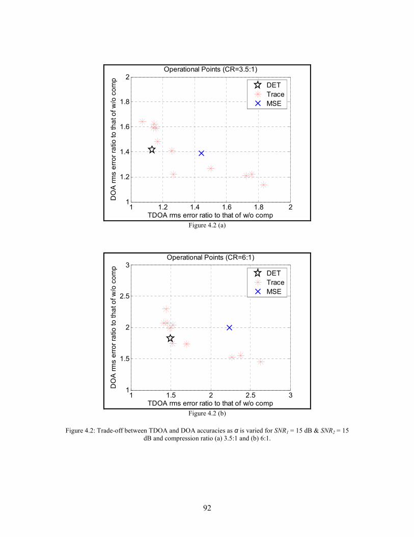
92

1 1.2 1.4 1.6 1.8 21

1.2

1.4

1.6

1.8

2

TDOA rms error ratio to that of w/o comp

DOA rms error ratio to that of w/o comp

Operational Points (CR=3.5:1)

DET

Trace

MSE

Figure 4.2 (a)

1 1.5 2 2.5 31

1.5

2

2.5

3

TDOA rms error ratio to that of w/o comp

DOA rms error ratio to that of w/o comp

Operational Points (CR=6:1)

DET

Trace

MSE

Figure 4.2 (b)

Figure 4.2: Trade-off between TDOA and DOA accuracies as α is varied for SNR1 = 15 dB & SNR2 = 15

dB and compression ratio (a) 3.5:1 and (b) 6:1.

93

3 3.5 4 4.5 5 5.5 61

1.5

2

2.5

3

3.5TDOA Performance

CR

RMS TDOA Error ratio to that of w/o. comp

TDOA only

DOA only

MSE

DET

Figure 4.3 (a)

3 3.5 4 4.5 5 5.5 61

1.5

2

2.5DOA Performance

CR

DOA Error ratio to that of w/o comp.

TDOA only

DOA only

MSE

DET

Figure 4.3 (b)

Figure 4.3 Effect of compression ratio on (a) TDOA and (b) DOA performance.

94

)())2/(()(

)())2/(()(

2

)2/(

02

1

)2/(

01

0

0

twettstx

twettstx

tj

tj

+−−=

++−=+

+

νν

νν

τ

τ (4.27)

The TDOA Fisher information measure is

,][2 2

1

22/

2/2

1

2

2

11 mSmN

JN

Nm

∑−=

=σπ

(4.28)

where S1[m] is the DFT of the signal at sensor S1 and the FDOA Fisher information

measure is

,][2

2/

2/

21

2

21

2

22 ∑−=

=N

Nn

nsnJσ

π (4.29)

where s1[n] is the signal data at sensor S1.

Equations (4.28) and (4.29) provide the formulas for computing the FI for the TDOA

only and FDOA only. Similar to joint TDOA/DOA estimation, compression requirements

for TDOA and FDOA are also conflicting because the TDOA Fisher information depends

on the DFT coefficients (with the DFT frequencies running over both negative and

positive frequencies) while the FDOA Fisher information depends on the signal samples

themselves. However, unlike the joint TDOA/DOA estimation where the compression

can be performed using the TDOA-only ON transform, the optimal ON transform for

TDOA is the DFT whereas optimal transform for FDOA is the identity matrix. Each DFT

coefficient is the combined result of all the time samples (from the beginning to the end),

similarly, one time sample is the combined result of all the DFT coefficients (from the

negative frequency to positive frequency). Even worse, the off-diagonal terms of the FIM

depend on both frequency-domain characteristics and time-domain characteristics. It is

difficult to calculate and optimize the post-compression values of all the components of

95

the FIM jointly unless we transform the data x1[n] into a time-frequency representation

where frequency resolution and time resolution are jointly provided. Wavelet packet

transform is such choice because it provides not only the time-frequency resolution that is

needed for our joint TODA/FDOA, but also provides the energy compactness which is

important for the compression efficiency.

Given an orthonormal wavelet packet basis set nψ with coefficients nc for the

data vector x1, we wish to select a subset Ω of coefficient indices and an allocation of bits

| Ω∈= ibB i to those selected coefficients such that the selected/quantized signal

∑Ω∈

=i

iicψ~~

1x , where |~ Ω∈ici are the quantized version of the selected coefficients. The

selection/quantization is to be done so as to maximize the post-compression values of

( ) 2211 1wtr JJ αα −+=J and detJ while meeting a constraint on the total number of

bits.

In principle, it is possible to write a mathematical equation for the coefficients and

then consider the derivatives with respect to parameters, as needed for the FIM. This,

however, quickly becomes intractable. Thus, we resort to exploiting the relationships

among the wavelet coefficients and DFT coefficients and original time-domain samples

of x1. Although it is impossible to relate each coefficient to a single DFT coefficient or

single time-domain samples, as shown in [81], [82], and [83], all wavelet coefficients in

the same band have the tendency to be associated only with a certain frequency range and

a block of adjacent wavelet coefficient in the same band have a tendency to correspond to

the same time range. Therefore, we can divide the wavelet coefficient into small blocks,

and give each block a frequency weight and time weight according to the time-frequency

96

location characteristic of wavelets. Besides providing us the reasonable time-frequency

resolution for compression for joint TDOA/FDOA estimation, operations on blocks of

coefficients, instead of coding coefficients individually, brings us computational

efficiency as well. Now consider that the wavelet packet coefficients ci are grouped into

M blocks, where each block contains coefficients at the same frequency and over a short

contiguous temporal range. The diagonal element of the FIM can be computed (up to a

multiplicative factor) as:

∑∑

=

∈

+=

M

j j

blockji

ij

q

cf

J1

22

1

22

11 σ (4.30)

∑∑

=

∈

+=

M

j j

blockji

ij

q

ct

J1

22

1

22

22 σ. (4.31)

where j is the block index, fj and tj are the frequency and central time, respectively, of

the jth block. Based on (4.30) and (4.31), the distortion measure for joint TDOA/FDOA

estimate can be determined in the following:

Weighted Trace Optimization:

The weighted-trace-based TDOA/FDOA distortion measure is then

∑∑

∑∑

+−+

+= ∈

=

∈M

j j

blockji

ijM

j j

blockji

ij

q

ct

q

cf

Jwtr22

1

22

122

1

22

)1())(~(

σα

σαα (4.32)

Bits are allocated to the coefficients using the method of [33] to maximize (4.32) for a

given rate constraint. To compare the proposed scheme with a traditional scheme, we also

97

allocated bits to the wavelet packet blocks to minimize MSE (2.36) under the bit

constraint.

Although the developed scheme is applicable to all varieties of signals, we use a

linear FM radar signal [87] to illustrate the method. A 3-level wavelet packet transform is

performed and 8 subbands are produced; each subband is partitioned into 8 blocks.

Moreover, to focus attention on the lossy compression performance, no entropy coding is

applied after quantization.

Simulation results are shown in Figure 4.4 and Figure 4.5. In Figure 4.4 we see the

inherent trade-off that is controlled by the choice of α, whose value controls whether the

algorithm favors TDOA accuracy, FDOA accuracy, or balances them to achieve the

closest operation to the no compression case. Figure 4.5 illustrates how changing the

compression ratio affects the TDOA and FDOA accuracy under several scenarios: the

results labeled “Goal Attained” illustrate the performance when the impact on TDOA and

FDOA is balanced. In these figures the advantage of using our distortion measures is

made clear.

Determinant Optimization:

Unlike the weighted trace, the other approach, maximizing the determinant, does not

provide us the flexibility to weight the relative importance between TDOA and FDOA

However, it takes into account the off-diagonal elements of J that the weighted trace

ignores and has the advantage of maximizing the size of the FIM ellipse. It is possible for

determinant optimization to automatically achieve the best tradeoff between TDOA

accuracy and FDOA accuracy without heuristically deciding the weight α in the

weighted trace approach. Correspondingly, the vector G needed to be used in (4.5)-(4.9)

98

Figure 4.4: Trade-off between TDOA and FDOA accuracies as α is varied for compression ratio 3:1 and

SNR1 = 15 dB & SNR2 = 15 dB; symbol denotes the operational point (α=0.5) closest to that without compression.

Figure 4.5 (a)

99

Figure 4.5 (b) Figure 4.5: Effect of compression ratio on (a) TDOA and (b) FDOA performance. A comparison is also

made to the case of simply sending less data (“Length Reduced”) rather than compressing the data.

Figure 4.6: Comparison between the determinant optimization method (‘Area’) and weighted trace method

(‘Premeter’) and MSE for compression ratio 3:1 and SNR1 = 15 dB & SNR2 = 15 dB;

1 1.2 1.4 1.6 1.8 2 2.20.9

1

1.1

1.2

1.3

1.4

1.5

1.6

1.7

TDOA RMS Error (w.r.t. w/o comp)

FDOA RMS Error (w.r.t. w/o comp)

"Primeter"

"Area"

w/o Comp.

MSE

100

can be determined by

=

∂

∂

∆∂

∂=

M

M

M

M

][][11 icticfv

jjjj

ssG ,

where ][ic j denote the wavelet coefficients residing in the jth block.

Simulation results are shown in Figure 4.6, where the weighted trace method is also

given for comparison; as expected, the operating point obtained from the determinant

method is the point to achieve the pareto optimal point (the closest operation to the no

compression case).

4.1.2 Modified Distortion Measures to Include Off-Diagonals

For the TDOA/FDOA-based location problem the estimation of TDOA/FDOA is only

a preliminary task; the real task is estimation of the geo-location of the emitter and that,

as is shown below, depends on the off-diagonals of the TDOA/FDOA FIM. For

simplicity we consider only 2-D geolocation.

The 2-D location estimate of the emitter Tee yx ]ˆ,ˆ[ˆ =x is sought and K pairs of sensors

are used. Each pair of sensors is able to measure both TDOA and FDOA so that we have

the measurements

Kiwfv

wf

i

i

viFDOAi

iTDOAi

,,2,1)(

)(

,

,

K=+=

+=

x

x ττ (4.33)

where i

wτ and iv

w are the random TDOA and FDOA measurement errors at the ith pair of

sensors, respectively. Any two measurements at a pair of sensor can be written as a single

equation for a 2-dimensional column vector.

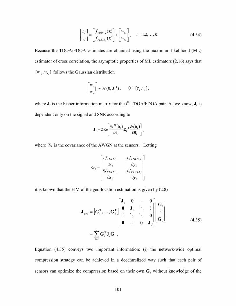
101

+

=

i

i

viFDOA

iTDOA

i

i

w

w

f

f

v

ττ)(

)(

,

,

x

x, Ki ,,2,1 K= . (4.34)

Because the TDOA/FDOA estimates are obtained using the maximum likelihood (ML)

estimator of cross correlation, the asymptotic properties of ML estimators (2.16) says that

],[ii vn ww follows the Gaussian distribution

),0(~ 1−

i

vi

i

w

wJN

τ, ],[ ii vτ=θ ,

where Ji is the Fisher information matrix for the ith TDOA/FDOA pair. As we know, Ji is

dependent only on the signal and SNR according to

( ) ( )

∂∂

∂∂

= −

i

ii

i

iH

iθ

θsΣ

θ

θsJ 1Re2 ,

where iΣ is the covariance of the AWGN at the sensors. Letting

∂

∂

∂

∂

∂

∂

∂

∂

=

e

iFDOA

e

iFDOA

e

iTDOA

e

iTDOA

i

y

f

x

f

y

f

x

f

,,

,,

G

it is known that the FIM of the geo-location estimation is given by (2.8)

[ ]

.1

1

2

1

1

∑=

=

=

J

i

iii

J

J

Jgeo

GJG

G

G

J00

0

J0

00J

G,,GJ

T

TT M

L

OOM

MO

L

L

(4.35)

Equation (4.35) conveys two important information: (i) the network-wide optimal

compression strategy can be achieved in a decentralized way such that each pair of

sensors can optimize the compression based on their own iG without knowledge of the

102

operations of other pairs of sensors; (ii) besides the TDOA/FDOA accuracies, the

location estimation accuracy also strongly depends on the geometry of the emitter and the

sensors [66]. For the 2-D X-Y location case, the 2×2 location error covariance matrix can

be replaced by 1−= geoJP [66]. Diagonalizing 1−P (or geoJ ) using

, 1

2

1

1

−−− = λλdiagAPA1T

and letting m)(ξAζT −= , where m is the real location of

target, leads to

2

κζ

:ξ1i i

2

i ≤= ∑= λ

R , (4.36)

where region R is the interior of the error ellipse with the ith principal axes length of

2(κλi)½.

In most sensor-target geometries, the relative importance of TDOA and FDOA is set

by the target-sensors geometry. Figure 4.4 and Figure 4.6 show how α controls the

compression trade-off between the TDOA and FDOA accuracies achieved by our method.

However, to choose a proper value of α requires knowledge of the target’s location –

which, unfortunately, is precisely what we are trying to estimate. However, we can first

send a small amount of data – enough to roughly determine the geometry; then that rough

geometry can be used to estimate an appropriate α value that would be fed back to the

compressing sensor and used to compress the remainder of the signal. In fact, this can

even be done to provide repeated updates of α as more data is compressed and sent; this

corresponds to updating the operating point along the curve shown in Figure 4.4 and

Figure 4.6.

103

This directly leads to the following simple scheme (not the only one) where the

compression can be adapted to the geometry. The scheme is shown in Figure 4.7, where

circled numbers correspond to the actions of the steps described below.

Step 1: The central node determines the compression ratio and its associated operational

compression points based on the requirement of energy consumption and latency. Then it

randomly picks J pairs of nodes to get J measurements of TDOA and FDOA. In the

beginning, one of the nodes J1),1,( ≤≤ ii sends a small length of its data to the other )2,(i ,

where rough measurements of TDOAs ~ , idτ and FDOAs ~ ,idv are measured.

Step 2: ~ , idτ and ~ ,idv are sent to the central node, where the rough prediction of the

geometry matrix G is estimated.

Step 3: In term of the estimated geometry matrix G, the central node determines the

optimal α and informs the nodes )1,(i about this choice and the compress ratio.

Step 4: The nodes )1,(i compress the data according the compression ratio and the chosen

α and send the compressed version of its sensed data to the nodes )2,(i .

Figure 4.7: Geometry Adaptive TDOA/FDOA System Scheme.

104

Step 5: The nodes )2,(i measure the , idτ and ,idv with the received data from node

)1,(i in Step 1 and decompressed data in Step 4. The resulting , idτ and ,idv are sent to

the central node, where the final location of the target is determined.

Simulations were performed as follows: A target can appear anywhere in a 2-D 5x5

km2 area, within which a large number of sensors is spread. Four sensors are randomly

picked to form two pairs to estimate TDOA/FDOA. 256 samples are sent in Step 1 to

roughly estimate the geometry. Finally, 4096 samples are compressed and shared

between each pair. For comparison, the 4096 data samples are compressed using the

MSE measure. In the simulation, we use the ratio of the area of circular error probable

(CEP) [66] with compression to that without compression minus 1 (which corresponds to

the relative increase in CEP) as the metric. CEP is estimated by 2175.0 λλ + [66]. There

were 2000 Monte Carlo runs performed for each compression ratio and the average

values are shown in Figure 4.8 . Over the range of compression ratio values considered,

the results in Figure 4.8 show a roughly 5x improvement in CEP for our method relative

to one that uses the wavelet packet transform but optimized according to MSE.

Actually, this geometry adaptive algorithm is optimized with respect to the FIM

of iτ and iv given a chosen α for each pair of sensor. Although the significant

improvement is achieved over MSE as shown in Figure 4.8, there is a step left to claim

that it is optimal with respect to FIM of ex and ey . As shown in (4.35). The correct

usage of the viable “Perimeter of the FIM” idea to optimizing compression with respect

to geo-location should be to compress to minimize the trace of

)tr()tr()ˆ()ˆ( 1−==−+− geoeeee yyxxE JP ; as before, instead of minimizing )tr( 1−geoJ , we

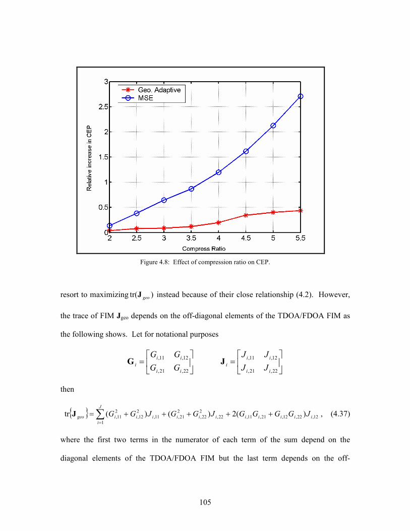
105

Figure 4.8: Effect of compression ratio on CEP.

resort to maximizing )tr( geoJ instead because of their close relationship (4.2). However,

the trace of FIM Jgeo depends on the off-diagonal elements of the TDOA/FDOA FIM as

the following shows. Let for notational purposes

=

=

22,21,

12,11,

22,21,

12,11,

ii

ii

i

ii

ii

iJJ

JJ

GG

GGJG

then

∑=

+++++=J

i

iiiiiiiiiiigeo JGGGGJGGJGG1

12,22,12,21,11,22,

2

22,

2

21,11,

2

12,

2

11, )(2)()(tr J , (4.37)

where the first two terms in the numerator of each term of the sum depend on the

diagonal elements of the TDOA/FDOA FIM but the last term depends on the off-

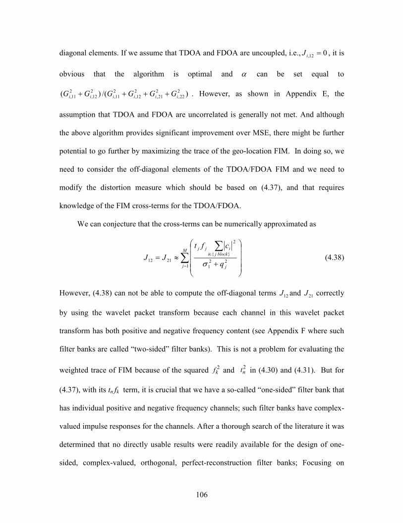
106

diagonal elements. If we assume that TDOA and FDOA are uncoupled, i.e., 012, =iJ , it is

obvious that the algorithm is optimal and α can be set equal to

)/()( 2

22,

2

21,

2

12,

2

11,

2

12,

2

11, iiiiii GGGGGG ++++ . However, as shown in Appendix E, the

assumption that TDOA and FDOA are uncorrelated is generally not met. And although

the above algorithm provides significant improvement over MSE, there might be further

potential to go further by maximizing the trace of the geo-location FIM. In doing so, we

need to consider the off-diagonal elements of the TDOA/FDOA FIM and we need to

modify the distortion measure which should be based on (4.37), and that requires

knowledge of the FIM cross-terms for the TDOA/FDOA.

We can conjecture that the cross-terms can be numerically approximated as

∑∑

=

∈

+≈=

M

j j

blockji

ijj

q

cft

JJ1

22

1

2

2112 σ (4.38)

However, (4.38) can not be able to compute the off-diagonal terms 12J and 21J correctly

by using the wavelet packet transform because each channel in this wavelet packet

transform has both positive and negative frequency content (see Appendix F where such

filter banks are called “two-sided” filter banks). This is not a problem for evaluating the

weighted trace of FIM because of the squared 2kf and

2nt in (4.30) and (4.31). But for

(4.37), with its tn fk term, it is crucial that we have a so-called “one-sided” filter bank that

has individual positive and negative frequency channels; such filter banks have complex-

valued impulse responses for the channels. After a thorough search of the literature it was

determined that no directly usable results were readily available for the design of one-

sided, complex-valued, orthogonal, perfect-reconstruction filter banks; Focusing on

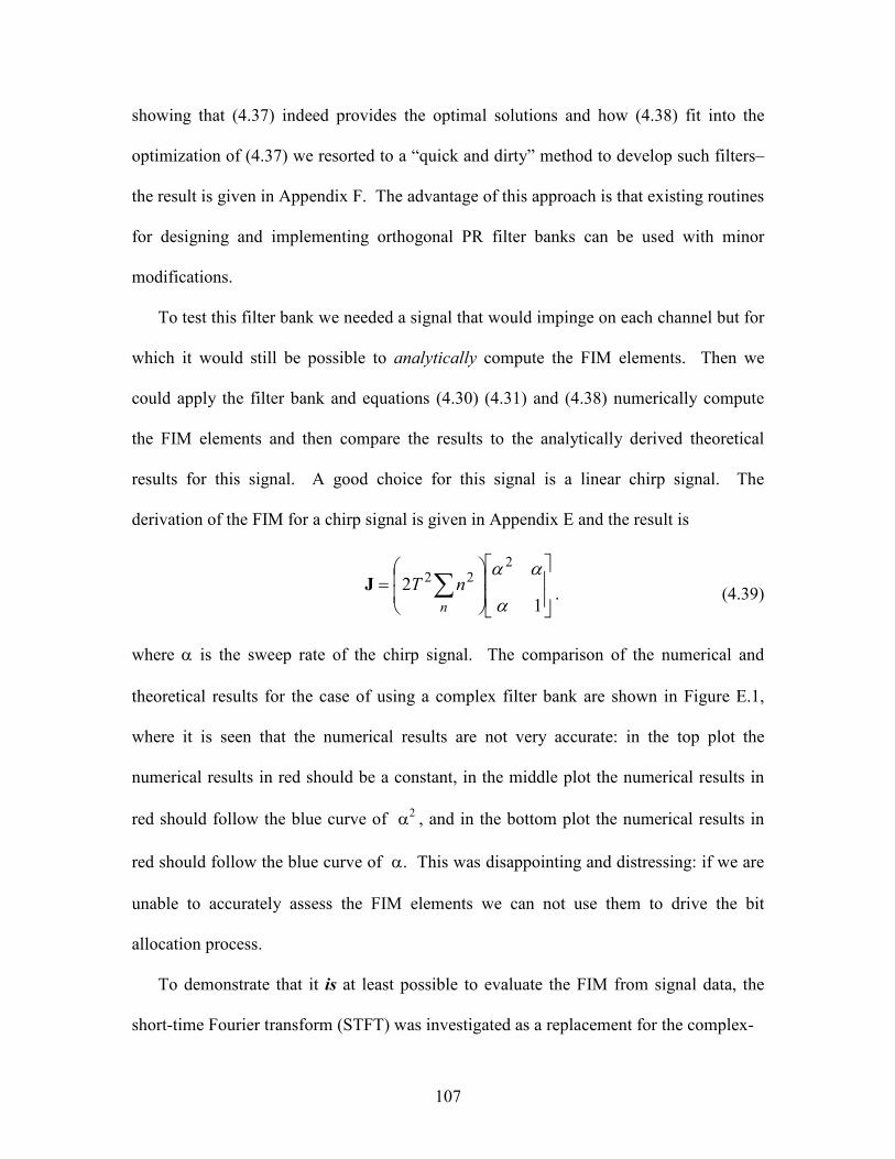
107

showing that (4.37) indeed provides the optimal solutions and how (4.38) fit into the

optimization of (4.37) we resorted to a “quick and dirty” method to develop such filters–

the result is given in Appendix F. The advantage of this approach is that existing routines

for designing and implementing orthogonal PR filter banks can be used with minor

modifications.

To test this filter bank we needed a signal that would impinge on each channel but for

which it would still be possible to analytically compute the FIM elements. Then we

could apply the filter bank and equations (4.30) (4.31) and (4.38) numerically compute

the FIM elements and then compare the results to the analytically derived theoretical

results for this signal. A good choice for this signal is a linear chirp signal. The

derivation of the FIM for a chirp signal is given in Appendix E and the result is

= ∑

1

2

222

α

αα

n

nTJ. (4.39)

where α is the sweep rate of the chirp signal. The comparison of the numerical and

theoretical results for the case of using a complex filter bank are shown in Figure E.1,

where it is seen that the numerical results are not very accurate: in the top plot the

numerical results in red should be a constant, in the middle plot the numerical results in

red should follow the blue curve of α2 , and in the bottom plot the numerical results in

red should follow the blue curve of α. This was disappointing and distressing: if we are

unable to accurately assess the FIM elements we can not use them to drive the bit

allocation process.

To demonstrate that it is at least possible to evaluate the FIM from signal data, the

short-time Fourier transform (STFT) was investigated as a replacement for the complex-

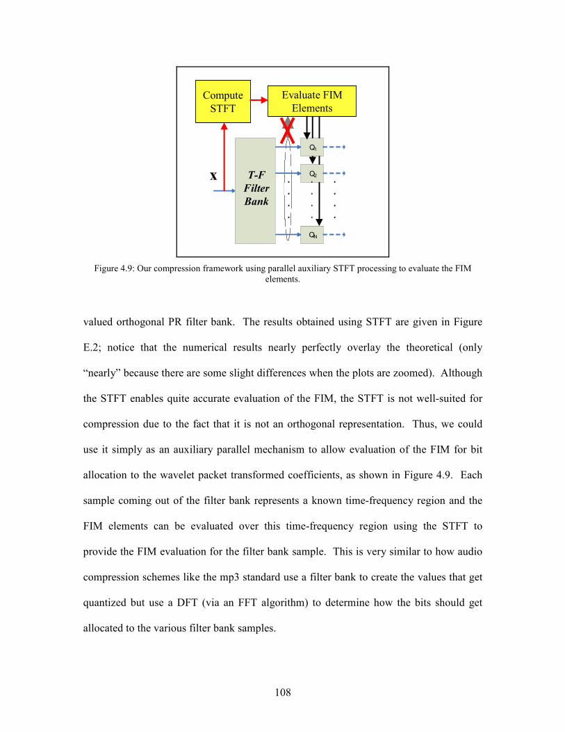
108

x

Q1

Q2

QN

Evaluate FIM

Elements

T-F

Filter

Bank

Compute

STFT

Figure 4.9: Our compression framework using parallel auxiliary STFT processing to evaluate the FIM

elements.

valued orthogonal PR filter bank. The results obtained using STFT are given in Figure

E.2; notice that the numerical results nearly perfectly overlay the theoretical (only

“nearly” because there are some slight differences when the plots are zoomed). Although

the STFT enables quite accurate evaluation of the FIM, the STFT is not well-suited for

compression due to the fact that it is not an orthogonal representation. Thus, we could

use it simply as an auxiliary parallel mechanism to allow evaluation of the FIM for bit

allocation to the wavelet packet transformed coefficients, as shown in Figure 4.9. Each

sample coming out of the filter bank represents a known time-frequency region and the

FIM elements can be evaluated over this time-frequency region using the STFT to

provide the FIM evaluation for the filter bank sample. This is very similar to how audio

compression schemes like the mp3 standard use a filter bank to create the values that get

quantized but use a DFT (via an FFT algorithm) to determine how the bits should get

allocated to the various filter bank samples.

109

4.1.3 Simulations of Compression Using Parallel Auxiliary STFT Processing

The idea and implementation of using parallel auxiliary STFT processing shown

in Figure 4.9 will be further exploited in this section through simulations. Two typical

geometries of the two pair of sensors and emitters are chosen to illustrate the

improvement obtained by accurate assessment of FIM. These two geometries are shown

in Figure 4.10 (a) and Figure 4.11 (a), respectively. Figure 4.10 (a) corresponds to the

case when TDOA and FDOA are both important for the location of emitter, while Figure

4.11 (a) corresponds to the case when FDOA is more important for one pair of sensor

while both TDOA and FDOA are important to the other pair. The Jacobian matrix 1G and

2G in (4.36) for Figure 4.10 are2:

=

8425.01728.2

5157.18314.11G and

−=

6003.21224.2

4777.2255.32G .

Similarly, the Jacobian matrix 1G and 2G in (4.36) for Figure 4.11 are

−−=

3697.01369.1

4077.03372.01G and

−

−−=

6357.13836.1

1011.29176.02G

Simulation results are shown in 4.10 (b) and 4.11 (b), where the trace of the practical

error covariance matrix of location is used to compare different algorithms under

investigation. STFT-WP FIM is the wavelet packet transform coding that uses parallel

auxiliary STFT to evaluate the FIM while WP FIM is the wavelet packet transform

coding that directly use equations (4.30) , (4.31) and (4.3) to compute the elements of the

FIM. Clearly, STFT-WP FIM is slightly better than WP FIM while both achived

2 ( 1G and 2G incorporate the mismatched units factor (TDOA error is in the unit of ns and FDOA error is

in the unit of Hz) or other factors determining the functions in (4.33). (See [66] and [84] for details)

110

significant improvement over the wavelet transform coding based on MSE. Results

marked wtr FIM represent the performance of the wavelet packet transform coding that is

based on the weighted trace distortion measure in (4.32). The wtr FIM ignores the off-

diagonal element 12,iJ and chooses α as )/()( 2

22,

2

21,

2

12,

2

11,

2

12,

2

11, iiiiii GGGGGG ++++ .

According to the Schwarz inequality, 22,

2

22,

2

21,11,

2

12,

2

11, )()( iiiiii JGGJGG +++ is greater

than or equal to 12,22,12,21,11, )(2 iiiii JGGGG + , which means that the on-diagonal elements of

geoJ dominant the off-diagonal elements and it might be good enough to use only wtr

FIM because it is much simpler than STFT-WP FIM. This is verified by Figure 4.10. (b)

and Figure 4.11. (b) where wtr FIM is very close to the optimal performance represented

by STFT-WP FIM.

4.2 Data Compression for Parameter Estimation with Detection

There might be a scenario where sensor 2S uses its own data and the decompressed

data from 1S to first detect the presence of a signal and then estimates the parameter of

interest. We can derive the Chernoff-distance based distortion. However, based on the

framework we used for multiple estimation tasks, it is not difficult to derive the following

Fisher-information-Matrix-Chernoff-Distance-based distortion measure to guide the

compression algorithm:

[ ] ∑=

≤×−+×N

n

isB

Rbtosubject1

11 )()1())((max xxJ µβψβ , (4.40)

where ψ represents any form of the FIM measures in 4.1 and β is a parameter used to

control the relative importance of estimation accuracy and detection error.

111

0 50 100 150 200 250 300 350 400 450 5000

50

100

150

200

250

300

350

400

450

500

X (m)

Y (m)

Geometry #1

Figure 4.10 (a)

2 3 4 5 6 7 80

0.1

0.2

0.3

0.4

CR (n:1)

Trace(P)

Trace of Geo-Location Error Covariance

STFT-WP FIM

WP FIM

w/o comp.

wtr FIM

MSE

Figure 4.10 (b)

Figure 4.10, (a) Geometry among the two pair of sensors and emitter, “*” represents the emitter and “o”

represent the sensors, and “---” denotes the wireless communication channel between each pair of sensors.

(b) The comparison of difference compression algorithms on the trace of error covariance of emitter

location.

112

0 50 100 150 200 250 300 350 400 450 5000

50

100

150

200

250

300

350

400

450

500

X (m)

Y (m)

Geometry #2

Figure 4.11 (a)

2 3 4 5 6 7 80

0.5

1

1.5

2

2.5

3

3.5

4

CR (n:1)

Trace(P)

Trace of Geo-location Covariance

STFT-WP FIM

WP FIM

w/o comp.

wtr FIM

MSE

Figure 4.11 (b)

Figure 4.11, (a) Geometry among the two pair of sensors and emitter, “*” represents the emitter and “o”

represent the sensors, and “---” denotes the wireless communication channel between each pair of sensors.

(b) The comparison of difference compression algorithms on the trace of error covariance of emitter

location.

113

For example, consider detecting the presence of a signal and then estimating TDOA

between a pair of sensors in the presence of AWGN. The distortion measure for

detection happens to coincide with the distortion measure for DOA. In other words, the

compression algorithm for DOA should be almost identical to that for detection except

for slight differences. Therefore the simulations used for testing the joint TDOA/DOA

application can be applied to the joint TDOA and detection without any changes except

that we replace weight α with β . Due to this reason and the reason that the usage of

(4.39) will be further discussed later in the compression for sequential inference task

application, we will postpone the simulations until the next chapter.

114

CHAPTER 5

Data Compression for Sequential Task of Multiple Inference Quantities

Recall the geometry-adaptive compression algorithm that we developed for joint

TDOA/FDOA estimation, it requires that either a small amount of initial data or very

coarse compressed data to be shared first to get a rough estimate of the emitter’s location,

if the rough estimate is inside the predicted error surface, it is possible to determine the

proper TDOA/FDOA trade-off for compressing and sharing the remaining data and

refining the rough estimate to a much more accurate estimate that satisfies the

requirement of the sensor system. On the other hand, if the rough estimate is far away

from our projected error surface, the fusion sensor can determine that the sensor has not

enough valuable information and no further sharing is needed. A similar scenario is the

sequential detect-then-estimate problem, where some compressed data is sent for the

detection task; once detected, the fusion center will require more data sharing among the

sensors to complete some estimation tasks. From these two examples, we can see that in

sensor networks, the inference tasks, rather than occurring simultaneously, are more

likely to happen sequentially for achieving the maximal information gain under the

energy and time constraint. Generally, the carrying out of major inferences of interest

could be preceded by conducting some “preliminary” inference which offers the central

information fusion center rough information about the process under investigation, since

115

in the complete absence of prior information, global optimization of the inference is

impossible. These preliminary inference results can be either deciding if the target is

present or roughly estimating of the geometry among the sensors and target. Then, after

estimates of the parameters are found, it is necessary to verify whether or not the

accuracy of the ultimate inference task at hand is sufficient, then depending on the

circumstances of sensor networks, the information fusion center must either stop or

design supplementary inference tasks for estimating the entire collection of parameters or

some group of them which are of more interest. As we know, the compression

requirements for the different inference tasks at each sequential stage are different and,

usually, conflicting. Therefore, optimized compression to handle sequential inference

tasks requires what we call “task-embedded compression”: the transmitting sensor

constructs the optimal task-embedded data stream to send only the data needed to

supplement the already-delivered data for optimal processing for the current task at each

stage. Although task-embedded compression is similar to the traditional embedded

coding compression technique, they are quiet different in principle since the data stream

of traditional embedded coding is constructed based on a single task (reconstruction) and

cannot be adapted for different requirements for different tasks. In the following, we will

first use a simple detection-then-TDOA sequential inference problem to illustrate our

task-embedded compression approach, then generalization to the general case is given.

5.1 Simple Detection-Then-TDOA Problem

Consider the scenario where multiple sensors are deployed to detect and then locate

RF emitters (e.g., communication or radar transmitters). At first the sensors would share

their collected data for the purpose of detecting when they have jointly intercepted a

116

common signal. After detecting the presence of an emitter, data is then shared among the

sensors to estimate the emitter’s position using the TDOA method. In these two

sequential stages, our task-embedded compression can be applied as follows: (i) the data

stream that is shared during the detection phase is optimally compressed for detection,

then (ii) the additional data “layer” needed to optimally estimate TDOA is sent.

For Gaussian noise, the compression distortion measures for the detection task are

(3.66)-(3.67) that depend on the SNR of post-compressed data while the distortion

measures for TDOA are based on its FI in (3.28)-(3.31) that depend on the quadratically-

frequency-weighted DFT coefficients. Suppose that two bit rates RD,1 and RE,1 for the

detection task and the estimation task are given, respectively. We can think of these two

rates as specifying corresponding resource consumption, resource-for-detection UD,1 and

resource-for-estimation UE,1, respectively, where the resource consumption means some

combination of energy and time whose exact form is up to different network design

criteria. Suppose further that optimizing the two tasks independently for their given

allocations yields a corresponding probability-of-miss (PM,1) and estimation error

standard deviation (σE,1) 1

. We can visualize the scenario in terms of these performance

measures as shown in the “conceptual” plots shown in Figure 5.1. The top plot on the

left in this figure shows the magnitude-squared DFT of the signal and the noise floor… to

maximize SNR for the detection task, the most important data is the DFT coefficients that

have magnitude-squared values above the noise floor. Suppose that the region shaded in

blue in the top plot is the optimally selected DFT coefficients for detection given the rate

1 We use probability-of-miss here (rather than the related probability-of-detection) so that the performance

measures for detection and estimation each have the characteristic of “bigger is bad, smaller is good”.

117

f 2 |S( f )|2

f

|S( f )|2

Noise

f

Sequential Tasks… Initial Trade-Off

Detect Source Estimate TDOA

PM < Limit (PFA = Desired)

Resouce-to-Detection < Limit

RMS Error < Limit

Resource-to-Estimation < Limit

σσσσEPM

PM,1

σσσσE,1

UD,1 UE,1

Figure 5.1: Sequential Tasks with the Initial Trade-Off.

constraint RD,1. The bottom plot on the left in the figure shows the quadratically-

weighted magnitude-squared DFT that drives the selection process for the TDOA-driven

compression. Suppose that the region shaded in solid blue in the bottom plot is the

optimally selected DFT coefficients for estimation given the rate constraint RE,1. Note

that the part that was previously sent for detection (shown in the bottom plot with striped-

blue shading) is already at 2S so it can be used for TDOA processing. The performance

trade-off is shown in the plot on the right of the figure. We take this performance as a

“baseline scenario” and see what else may be accomplished with respect to this baseline.

On the other hand, it should be noticed that an inherent tradeoff exists between different

stages. For example, if it is determined that the resource-for-estimate UE,1 is too much to

meet other important design requirement and has to be decreased while we want to keep

the estimation accuracy about the same and we wish to keep the resource-for-detection

UD,1 about the same. This can only be done by forcing the detection stage to send data

118

Sequential Tasks… New Trade-Off

f 2 |S( f )|2

f

|S( f )|2

Noise

f

σσσσEPM

PM,1

σσσσE,1σσσσE,2

UD,1UD,2

UE,1

PM,2

UE,2

Figure 5.2: Sequential Tasks with a New Trade-Off .

that would ultimately be helpful in the estimation stage with the consequence of the

degradation detection performance (an increase in the Probability-of-Miss). The top plot

of Figure 5.2 shows a heuristic way for this case where we remove some of the

previously selected DFT coefficients and include higher frequencies in the detection

selection set in the detection stage. The new chosen DFT coefficients should take about

the same number of bits (actually it would likely take fewer bits because of the smaller

amplitudes at these higher frequencies… but we’ll ignore that here). The vertical dashed

lines are the same as in the first scenario and simply show that we are now sending higher

frequency info during detection than we did before. In the bottom plot of Figure 5.2, the

solid yellow shows the new data that we need to send to support estimation… the striped-

yellow shaded data is what was already there from the detection task.

So the resource-for-estimation is decreased while the location accuracy will be about

the same. The detection performance will be worse but the resource-for-detection will be

about the same. This performance trade-off is shown on the right side of Figure 5.2,

where blue points indicate the initial trade-off scenario and the yellow points indicate the

new trade-off scenario. Note that the total resource for these two successive tasks has

119

also been reduced. (4.40) gives us the standard optimization methods for us to make

tradeoffs between detection and estimation and we can use it here in the detection stage.

This shows that there is a fundamental similarity between the simultaneous task case and

the sequential task case, compression algorithms for simultaneous algorithm (4.12), (4.15)

and (4.39) can be easily modified to give the following sequential algorithm.

5.1.1 An Algorithm for Sequential Detect-Then-TDOA

Detection stage 1: Maximizing SNR for the Detection Task according to (4.40)

D

N

n

n

N

Nn n

N

Nn nb

Rbbq

nX

bq

nXnMaximize

n

≤

+×−+

+× ∑∑∑

−

=−=−=

1

0

1

2/

2/22

22/

2/22

22

subject to

)(

][)1(

)(

][

111 σ

βσ

β

(5.1)

where X[n] is the DFT of the data, )(1

2nbq is the quantization noise power as a function of

the number of bits 1n

b allocated to that coefficient, DR is the rate for Stage 1, and the

parameter β controls the tradeoff between TDOA estimation and detection. The first

summation term in (5.1) measures the importance of a bit for TDOA estimation while the

second summation measures the importance of the bit for detection. Thus, setting β = 0

causes this allocation to be done with no consideration of the Stage 2 task of TDOA

estimation; however, increasing β forces more consideration of the subsequent Stage 2

task. Thus, instead of achieving trade-offs by the “discard-and-move” operations

described above, here the trade-off is achieved byβ .

Stage 2: Maximizing Fisher Information for the TDOA Estimation Task According

to (3.28)

In this stage only TDOA is of interest and its accuracy needs to be refined. Thus we

will maximize

120

E

N

n

n

N

Nn nnb

Rbbbq

nSnMaximize

n

≤

++∑∑−

=−=

1

0

2/

2/22

22

2

212

subject to)(

][

σ (5.2)

where ER is bit budget for the stage 2, and the 1nb are the bits already allocated in the

first stage.

5.1.2 Simulation Scenario

In terms of practical coding, unlike the simultaneous case, quantizers must be

changed to dead-zone uniform embedded quantizer in order to support the task-embedded

data stream between the sensors. Moreover, for the ease of implementation and testing,

we will focus on a trade-off scenario that is an alternative to that shown in Figure 5.2 ;

the case considered is shown in Figure 5.3 where the resourses for different tasks are held

fixed and only performance is changed during the trade-off: performance points move

along the vertical dotted lines. However, it should be pointed out that once this trade-off

is obtained, estimation bits could be discarded to decrease UE and increase σE,2; thus, this

new fixed-task-resource scenario can actually be made equivalent to the fixed-estimation-

accuracy/reduced-estimation-time scenario described above.

Sequential Tasks Trade-Off

σσσσEPM

PM,1

σσσσE,1

UD,1UD,2

UE,1

PM,2

UE,2

σσσσE,2

Could also Reach Points

Here w/o Changing

Detection Operating Point

Figure 5.3: Trade-off for fixed task resources .

121

For the simulation results below we imposed the conditions:

• During the first detection stage, in order to satisfy a resource constraint DU , the

data is compressed with a compression ratio of 8:1.

• During the second estimation stage, in order to satisfy a time constraint EU ,

Stage 2 bits are added such that the total compression ratio is 5:1.

As illustrated in Figure 5.4, the variation of the parameter β enables the tradeoffs

for the detection performance during the first detection stage and the location accuracy

during the second estimation stage. Actual simulation results are shown in Figure 5.5,

where the actual probabilities in the detection stage were not evaluated due to the fact

that such evaluations would take tremendous time. The results in Figure 5.5 show the

various SNR-σE points that can be achieved for fixed UD and UE; the points in the upper

right corner favor detection while those in the lower left corner favor estimation. Note

that the values of the post-compression detection-stage SNR were quite low; this is due to

the large compression ratio that was imposed. However, detection accuracy is not only

dependent on post-compression SNR but also on the size of data; any increase in SNR

indicates a significant decrease in error probability for large sample sizes (3.55). In

another point of view, it should be noted that this SNR is increased via the cross-

correlation by the time-bandwidth product, which generally is large enough to pull such

low SNR values up to an easily detectable level [5][69]. The specific operating values

shown in Figure 5.5 are of less importance than the fact that the simulation results verify

that the algorithm achieves a curve of trade-off points as expected.

122

Figure 5.4: Conceptual illustration of the trade-off accomplished via choice of the β parameter. Where

SNR1=SNR2=15 dB.

1.3 1.35 1.4 1.45 1.5 1.551.25

1.3

1.35

1.4

1.45

1.5

1.55

1.6

Figure 5.5: Simulation results illustrating the achieved trade-offs.

5.2 General Sequential Data Compression Algorithm

Based on the detection-then-TDOA example, the general idea of task-embedded

compression is very clear. In the following, we extend it into the generalized case.

Without loss of generality, we assume there are only two stages and the ultimate goal is

to estimate the unknown vector ],,[ 1 pθθ K=θ or unknown r×1 vector )(θga = .

First Inference Stage (Detection or Rough Estimation):

123

In this stage, we either don’t know if the target is present or we have no priori

geometry to compress data optimally. Therefore, responding to different processes under

investigation, optimization of the compression algorithm can be any one of the following

three under the constraint that the summation of the bit allocation vector

],,[ 211 nn bbB L= is not greater than 1R .

1. Maximize the Chernoff distance ),( 11 Bs xµ for the detection purpose, i.e.,

∑−

= +=

1

022

2

11)(

),(max

11

N

n n

ns

B bq

SB

σxµ (5.2)

where nS is the ON transform of 1x .

2. Maximize the information utility function ψ of FIM for the rough estimation

purpose. ψ could be either determinant or trace2 as

( )

∑∑

∑∑

−

=

−

=

−

=

−

=

+

Γ

+

Γ

+

Γ

+

Γ

=

=

1

0 1

22

1

0 1

22

1

1

0 1

22

11

0 1

22

11

11111

1111111

11,1

)()(

)()(

),(ˆ),(ˆ

),(ˆ),(ˆ

),(ˆdetmax1

N

n n

pp

nN

n n

p

n

N

n n

p

nN

n n

n

ppp

p

B

bqbq

bqbq

BJBJ

BJBJ

B

σσ

σσ

L

MOM

L

L

MOM

L

xx

xx

xJ θ

(5.3)

( ) ∑∑∑=

−

== +

Γ==

p

i

N

n n

ii

np

i

iiB bq

BJB1

1

0 1

221

1111,1)(

),(ˆ),(ˆtrmax1 σ

xxJ θ (5.4)

2 We might only need to maximize determinant or trace of a sub-matrix of the Fisher information matrix,

corresponding to certain inference task of interest. Although weighted trace can be used too, due to

the lack of information to determine the weight α, we have to let us stay with the assumption that all

the inference tasks are equally important at the inference stage 1

124

where j

n

i

nij

n

SS

θθ ∂

∂

∂

∂=Γ .

3. Maximize the weighted combination of information utility function ψ of FIM

and Chernoff distance )( 1xµ s , i.e., ),()1()),(ˆ( 1111,1 BB sxµxJ θ ββψ −+ for

situation where the first stage is forced to send data that would ultimately be

helpful in the second stage.

Second Inference Stage (estimation refinement):

In this stage, central fusion sensor could determine the optimal strategy to do the

subsequent compression to refine the estimation given the known the presence of target

or priori knowledge for the relative importance of multiple estimate for a specific task

from the first stage. The compression can take one of the following two cases under the

constraint that the sum of the supplemental bit allocation vector [ ]2122 ,, nbbB K= is not

greater than 2R :

1. Only a single θ is of interest, we need to

( ) ∑∑∑=

−

== +

Γ==

p

i

N

n n

ii

nip

i

iiiB bq

BJB1

1

0 1

221

1111,2)(

),(ˆ),(ˆtrmax1 σ

αα xxJ θ ; (5.5)

2. The whole set parameter ],,[ 1 pθθ K=θ are of interest, we need to

++

Γ

++

Γ

++

Γ

++

Γ

∑∑

∑∑

−

=

−

=

−

=

−

=

GG ˆ

)()(

)()(ˆTracemax

1

0 12

22

1

0 12

22

1

1

0 12

22

11

0 12

22

11

B2 N

n nn

pp

nN

n nn

p

n

N

n nn

p

nN

n nn

n

T

bbqbbq

bbqbbq

σσ

σσ

L

MOM

L

, (5.6)

where G is the pr × Jacobian matrix θθ ∂∂= /)(ˆ gG estimated from the first stage.

125

Two more simulations are performed to exploit this task-embedded compression

algorithm. The first simulation is for the sequential multiple parameter estimation, where

in the first stage the determinant optimization algorithm is used to get a rough estimate of

TDOA/FDOA/DOA according to (5.3). Based on which, one of TDOA and FDOA and

DOA estimate is determined as the dominant parameter that needs refining. Then in the

second stage, subsequent compression for any one of TDOA or FDOA or DOA is

performed according to (5.5). The determinant method is chosen for the first stage

because it is more likely to produce the best tradeoff among three different location

methods, TDOA, FDOA, and DOA, which provide us with a good initial estimate of the

parameter when we have no prior information of the location of the emitter. The

compression ratio imposed on the first stage is 8:1, and bits are added in the second stage

until the total compression ratio is 5:1. Pre-compression SNR at the two sensors (SNR1

and SNR2 ) are both set as 15 dB. The effectiveness of this method is shown in Table 1.

The first three rows of Table. 1 correspond to roughly estimating TDOA/FDOA/DOA in

the first stage by maximizing determinant of FIM and refining only one single parameter

TDOA , FDOA and DOA in the second stages, respectively. The first three columns are

the error standard deviation for the rough estimation of TDOA (ns), FDOA (Hz) and

DOA (m oC) in the first stage, respectively and the last three columns are the final

estimation error standard deviation for TDOA, FDOA and DOA in the refining second

stage, where the shaded and underlined shows the final estimation error standard

deviation of the parameter wanted to be refined in the second stage. The estimation

accuracies for TDOA/FDOA/DOA without any compression are also shown in Table.1

for the comparison purpose. We can see that at the second stage, the accuracy of the

126

parameter of interest is very close to the case where no compression is performed. The

scheme of second simulation is same to the first one except that the detection is the

required task in the first stage and compression for maximizing SNR is performed instead

in this stage. The results are shown in Table 2.

Table 5.1, Sequential Example, Rough Multiple Estimate - Then- Refine Estimation

First Stage Compression Second Stage Compression

TDOA (S1)

FDOA (S1)

DOA (S1)

TDOA (S2)

FDOA (S2)

DOA (S2)

det(FIM) 1.7655 3.0168 0.10761 TDOA only 0.61107 1.8143 0.068

det(FIM) 1.8732 3.1543 0.10428 FDOA only 0.82308 1.5719 0.068

det(FIM) 1.8466 3.0799 0.1058 DOA only 0.825 1.8035 0.059

TDOA (w/o)

FDOA (w/o)

DOA (w/o)

0.51755 1.3621 0.0501

Table 5.2, Sequential Example, Detection-Then - Estimation

First Stage Compression Second Stage Compression

TDOA (S1)

FDOA (S1)

DOA (S1)

TDOA (S2)

FDOA (S2)

DOA (S2)

Detect 1.6472 3.1896 0.1005 TDOA only 0.6028 1.8306 0.0652

Detect 1.6388 3.2728 0.1000 FDOA only 0.8132 1.5575 0.0667

Detect 1.6132 3.1146 0.0973 DOA only 0.843 1.7125 0.0632

127

CHAPTER 6:

Conclusion

This dissertation addresses using data compression as the tool to improve the energy

efficiency and timeliness of wireless sensor networks for inference tasks

(estimation/detection). Firstly, investigations are performed to assert that compression

can be deployed as a powerful and effective tool for the optimal trade-offs between rate,

energy, and accuracy in the wireless sensor network; Secondly, instead of using the

traditional MSE distortion measure that is only weakly related to the quality of estimation

and detection tasks, we use distortion measures based on the Fisher information for

estimation tasks and the Chernoff-distance for detection; The new developed distortion

measures are able to better evaluate the underlying information embedded in the collected

data for estimation/detection. As demonstrated by exhaustive examples of practical

interest, the compression algorithms based on our proposed distortion significantly

outperform those based on MSE. Finally, although the sequential and simultaneous

inference tasks are typical in wireless sensor network applications, no other researchers

have ever addressed compression for these two issues for wireless sensor networks, and

even for networks of several macrosensors. We develop the theories and compression

algorithms for the general simultaneous estimation problem and joint estimation and

detection problem as well as the theories and algorithms for “task-embedded

compression” to support sequential multiple inference tasks. In all, this dissertation sets

up the whole compression structure for inference tasks in wireless sensor networks and

128

the results can be used as a key component of and incorporated into the task-driven

network management and sensor management.

Despite these accomplishments, there are still some details insides our framework for

which some further work are needed:

1. In Chapter 3, although the general FI and Chernoff distance of quantized

noisy measurements are formulated and are applicable to all types of noise

and quantizers, in this dissertation, for the purpose of simplicity, we limit our

focus mainly on the case when the noise is Gaussian noise and the quantizer is

uniform quantizer due to their widely usage in literature and propose the

corresponding approximation model, which is used as a replacement for the

true model in Chapter 4 and 5. Further exploitation of other type of noise will

definitely further strengthen our compression structure.

2. For compressions for estimation, in general the FIM can depend on the

parameter vector values, although in this dissertation, we limit ourselves to

some practical estimation problems the FIM does not depend on the parameter

values or at least the FIM can be separated into the part containing only the

unknown-parameter-centric part and the data-centric part containing to which

our “maximize Fisher information” approach can still be applied. However,

there may exist the case where the Fisher information depends on the

parameters which can not be pulled out of the data as in (3.43). We have

proposed the correct approach for this problem but have not yet fully explored

its application. Thus, some further research is needed to determine if there are

estimation problems for which the “maximize Fisher information” approach

129

can not be directly applied and then demonstrate how to attack them using the

minimax approach.

3. Regarding to the geometry adaptive algorithm for joint TDOA/FDOA

estimation, although we demonstrate that we can use parallel auxiliary STFT

to access the FIM elements and help the algorithm to evaluate the right

relative importance of wavelet packet coefficients to joint TDOA/FDOA

estimation. To improve the computational efficiency, Further works is still

needed to develop filter banks that are well-suited to both compression and

FIM evaluation

4. There are still some small details surrounding the detection problem, such as

instead of real probability of detection, we use the Chernoff distance as the

indication of detection. Although this is true from the theory, further work is

still needed to verify it.

5. Although a lot of effort is paid to choose and improve the computation

efficiency of compression algorithms to achieve maximal saving of time and

energy, further examination of the computational and implementation aspects

of the algorithm is still needed, and hardware implementation is desired in the

future.

130

APPENDICES

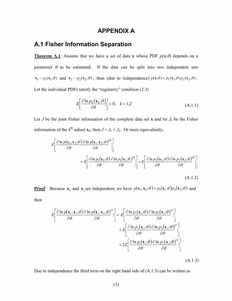
131

APPENDIX A

A.1 Fisher Information Separation

Theorem A.1: Assume that we have a set of data x whose PDF p(x;θ) depends on a

parameter θ to be estimated. If the data can be split into two independent sets

),(~ 111 θxx p and ),(~ 222 θxx p ; then (due to independence) ),(),(),( 2211 θθθ xxx ppp = .

Let the individual PDFs satisfy the “regularity” condition (2.3)

( )2,1,0

;ln==

∂

∂k

pE kk

θθx

. (A.1.1)

Let J be the joint Fisher information of the complete data set x and let Jk be the Fisher

information of the kth subset xk; then J = J1 + J2. Or more equivalently,

( ) ( )

( ) ( ) ( ) ( )

∂

∂

∂

∂+

∂

∂

∂

∂=

∂

∂

∂

∂

HH

H

ppE

ppE

ppE

θθ

θθ

θθ

θθ

θθ

θθ

;ln;ln;ln;ln

;,ln;,ln

22221111

2121

xxxx

xxxx

(A.1.2)

Proof: Because 1x and 2x are independent, we have ( ) ( ) ( )θθθ ;;;, 221121 xxxx ppp = and

then

( ) ( ) ( ) ( )

( ) ( )

( ) ( )

∂

∂

∂

∂+

∂

∂

∂

∂+

∂

∂

∂

∂=

∂

∂

∂

∂

H

H

HH

ppE

ppE

ppE

ppE

θθ

θθ

θθ

θθ

θθ

θθ

θθ

θθ

;ln;ln2

;ln;ln

;ln;ln;,ln;,ln

2211

2222

11112121

xx

xx

xxxxxx

(A.1.3)

Due to independence the third term on the right hand side of (A.1.3) can be written as

132

( ) ( ) ( ) ( )

∂∂

×

∂

∂=

∂∂

∂∂ HH

pE

pE

ppE

θθ

θθ

θθ

θθ ;~ln;~ln;~ln;~ln 22112211 xxxx

. (A.1.4)

and each term on the right hand side of (A.1.4) is zero due to the assumed regularity

condition. Thus, (A.1.3) reduces to (A.1.2) and the claimed result is proved.

A.2 Chernoff Distance Separation

Theorem A2: Consider a problem consisting of deciding between two hypothesis 0H

and 1H based on a set of observed random vectors x . Hypotheses 0H and 1H are (no

target) and (target present) hypothesis, respectively, and are represented by

)(~:

)(~:

11

00

xx

xx

pH

pH (A.1.5)

If the data can be split into two independent sets 1x and 2x , each of which follows

2,1),(~:

2,1),(~:

,11

,00

=

=

ipH

ipH

iii

iii

xx

xx. (A.1.6)

Let ))(),(( 10 xx ppsµ be the joint Chernoff distance of the complete data set x and let

))(),(( ,1,0 kkkks pp xxµ be the Chernoff distance of the kth subset xk; then =))(),(( 10 xx ppsµ

))(),(())(),(( 22,122,011,111,0 xxxx pppp ss µµ + . Or more equivalently,

∫∫∫

−

−− −−=−

222,1

1

22,0

111,1

1

11,01

1

0

)()(ln

)()(ln)()(ln

xxx

xxxxxx

dpp

dppdpp

ss

ssss

(A.1.7)

Proof: Because 1x and 2x are independent, we have ( ) ( ) ( )22,011,00 xxx ppp = and

( ) ( ) ( )22,111,11 xxx ppp = then

133

( )

∫∫∫∫

∫ ∫∫

−−

−−

−−−

−−=

−=

−=−

222,1

1

22,0111,1

1

11,0

222,1

1

22,0111,1

1

11,0

2122,1

1

22,011,1

1

11,01

1

0

)()(ln)()(ln

)()()()(ln

)()()()(ln)()(ln

xxxxxx

xxxxxx

xxxxxxxxx

dppdpp

dppdpp

ddppppdpp

ssss

ssss

ssssss

(A.1.8)

Thus the claimed result is proved.

134

APPENDIX B

B. 1: Fisher information of scalar quantized data

Let ( )nnnbnr ωθξ += )(Q , and n

pω denote the probability density function (PDF) of

nω . The thresholds of the scalar quantization of nχ it is illustrated in Figure2.3, where

nbM 2= . The probability of nr falling into the interval ],( 1t−∞ can be thereby calculated

as

( )( ) ( )

))(()(

)(Prob)(Prob

|Prob);(

1

)(

11

0

1

0

θξη

θξωωθξ

χθ

ω

θξ

ω n

t

nnnn

nnn

q

r

tdttp

tt

qrbf

n

n

n

n

−==

−<=<+=

==

∫−

∞−

, (B.1)

where nωη is the cumulative distribution function for PDF of nω and is defined as

( ) ∫ ∞−=

x

dttpxnn

)(ωωη . (B.2)

Similarly, the probability of nr falling into the interval ),[ 1 ∞−Mt are calculated as

( )( )

( ))(1)(

)(Prob

)(Prob);(

1)(

1

1

1

1

θξη

θξω

ωθξθ

ωθξ ω nMt

nMn

Mnnn

q

r

tdttp

t

tbf

nnM

n

M

n

−−==

−>=

>+=

−

∞

−

−

−

∫−

−

. (B.3)

Except for these two end points, all other probability in the interval [ )1, += jjj ttI can be

calculated as

( ) ( )( )

( ) ( ))()(

)(

)()(Prob

)(Prob|Prob);(

11

)(

)(

1

1][

1

θξηθξη

θξωθξ

ωθξχθ

ωω

θξ

θξ ω

njnj

t

t

njnnj

jnnjnjnn

q

kr

tt

dttp

tt

ttqrbf

nn

nj

njn

j

−−−=

=

−<<−=

<+<===

++

−

−

+

+

∫+

(B.4)

135

Applying Leibnitz’s rule, (B.1) yields

( )( ) ( )

θθξ

θξθ

θξηω

ω

∂∂

−−=∂

−∂ )())((

)(1

1 nn

ntp

t

n

n . (B.5)

(B.5) makes it possible to get the closed form of the Fisher information of any scalar

quantized data. With it, the derivative of (B.3) and (B.4) with respect to θ are

( ) ( )

θθξ

θξθ

θω ∂

∂−=

∂

∂−

− )())((

);(1

1

nnM

n

q

rtp

bf

n

M

n , (B.6)

( ) ( ) ( )

θθξ

θξθξθ

θωω ∂

∂−−−−=

∂

∂+

)())(())((

);(1

nnjnj

n

q

rtptp

bf

nn

j

n . (B.7)

Plug these results into (3.12), the Fisher information of nb bit quantized coefficient nχ

is

( )( )

( )( ) ( )

( )

−−

−+

−−−

−−−+

−

−

∂

∂=

−

−

−

= +

+∑

)(1

))((

)()(

))(())((

)(

))(()(),(

~

1

1

2

2

1 1

22

1

2

1

1

22

θξη

θξ

θξηθξη

θξθξ

θξη

θξ

θθξ

θ

ω

ω

ωω

ωω

ω

ω

nM

nM

M

q nqnq

nqnq

n

nnnr

t

tp

tt

tptp

t

tpbJ

n

n

nn

nn

n

n

n

. (B.8)

B. 2, Approximation model

Consider

εων += 1 (B.9)

where v is the N×1 vector of the summation of receiver noise and quantization noise,

and ε is the N×1 vector of quantization noise nε which is modeled as white and uniform

in the interval ]2/,2/[ ∆∆− , and 1ω is the N×1 vector of the white Gaussian noise

coefficients nω with zero mean and variance 2σ . Now, our question becomes how to

analyze the PDF of nv and approximate it properly.

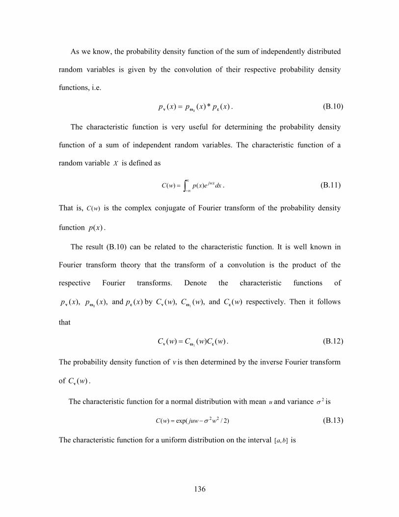
136

As we know, the probability density function of the sum of independently distributed

random variables is given by the convolution of their respective probability density

functions, i.e.

)(*)()( xpxpxp εωv 1= . (B.10)

The characteristic function is very useful for determining the probability density

function of a sum of independent random variables. The characteristic function of a

random variable X is defined as

∫∞

∞−= dxexpwC

jwx)()( . (B.11)

That is, )(wC is the complex conjugate of Fourier transform of the probability density

function )(xp .

The result (B.10) can be related to the characteristic function. It is well known in

Fourier transform theory that the transform of a convolution is the product of the

respective Fourier transforms. Denote the characteristic functions of

),(),( xpxp1ωv and )(xpε by ),(),(

1wCwC ωv and )(wCε respectively. Then it follows

that

)()()(1

wCwCwC εωv = . (B.12)

The probability density function of v is then determined by the inverse Fourier transform

of )(wCv .

The characteristic function for a normal distribution with mean u and variance 2σ is

)2/exp()( 22wjuwwC σ−= (B.13)

The characteristic function for a uniform distribution on the interval ],[ ba is

137

)2/)(exp())(2

1sin(

)(

2)( wbajwab

wabwC +−

−= (B.14)

Hence, we can calculate )(wCv by

)2/exp(2/

)2/sin()()()( 22w

w

wwCwCwCv σεε −

∆∆

== . (B.15)

The inverse Fourier transform of (B.15) is very complicate, but we can approximate

)(wCv as a Gaussian distribution

)2/exp()(~ 22wwC vv σ−= , 12/)var( 222 ∆+=+= σσ YXv (B.16)

under the condition that the null-to-null bandwidth of the characteristic function

)(wCq ∆/4π is larger than σ/6 , within which more than 99.7% of the area of the

characteristic function )(wCn is included.

Here we give some numerical results that show the effectiveness of the Gaussian

approximation used for the FI with multi-bit quantization. We assume that we have a set

of noise-free coefficients that lie in the range ±A. A noisy version of the coefficients

having additive Gaussian noise of variance 2σ is quantized to b bits using a mid-step

uniform quantizer with quantization cell size given by

2/12 1

22

−+

=∆ −B

A σ. (B.17)

By using our approximation condition, we can get how many bits are at least needed in

order for the approximation (B.16) to be valid.

3/2

/6/4

πσσπ

≤∆⇒

≥∆

138

12

1

2

13log

3

2

2/12

2

1

22

+

+

+≥⇒

≤−

+⇒

−

π

πσσ

PSNRB

AB

(B.18)

Under the inequality (B.18), we need 7.2≥B bits at 15 dB and 2≥B quantizer at

PSNR=10 dB (Uniform quantizer cannot quantize the signal with fractional bits,

therefore 3 bits is needed at PSNR=15 dB and 2 bits is needed at PSNR=10dB). If we

loosen the approximation condition of approximation (B.11) a little bit, i.e., instead of

constraining the mainlobe of )(wCq must contain 99.7% energy of )(wCn , we permit

some energy leakage of )(wCn and let the mainlobe of )(wCq ∆/4π include 95 energy of

)(wCn (that is, ∆/4π is larger than σ/4 ). In the later case, only a 2-bit quantizer is

needed at 15dB. The results provide motivation that at least for low PSNR the

approximation seems to be valid even down to the lowest number of bits for which it is

applied. For higher PSNR the approximations at 2 bits will be poorer;

Next, we plot the characteristic function to support the approximation model (B.16).

As illustrated in Figure B.1, the approximation is perfect when the quantizer is 3 bits and

PSNR is 15 dB. For 2-bit quantizer at PSNR=15dB, although there exists a little bit of

difference between the approximation and the true distribution, but it is still a pretty good

approximation. If the PSNR decreases to 10 dB, the condition for perfect performance of

the approximation model only needs 2-bit quantizers.

The validity of this approximation can be further tested analytically by comparing

the Fisher information under the approximation with its true expression in (B.8). For nb -

bit uniform quantization, the thresholds are nnn mmm ∆∆+−∆− ,,)1(, K , where

139

-40 -30 -20 -10 0 10 20 30 40

-0.4

-0.2

0

0.2

0.4

0.6

0.8

1Characteristic Function

Uniform Quantization

Gaussian Noise

Sum of above two

-40 -30 -20 -10 0 10 20 30 40-0.2

0

0.2

0.4

0.6

0.8

1Compare the true characteristic fucntion and the approximated one

True

Approximation

Figure B.1, (A)

-40 -30 -20 -10 0 10 20 30 40-0.4

-0.2

0

0.2

0.4

0.6

0.8



Gaussian NoiseSum of above two

-40 -30 -20 -10 0 10 20 30 40-0.2

0

0.2

0.4

0.6

0.8

1

1.2Compare the true characteristic fucntion and the approximated one

True

Approximation

Figure B.1 (B).

-40 -30 -20 -10 0 10 20 30 40-0.4

-0.2

0

0.2

0.4

0.6

0.8



Gaussian Noise

Sum of above two

-40 -30 -20 -10 0 10 20 30 40

-0.2

0

0.2

0.4

0.6

0.8

1Compare the true characteristic fucntion and the approximated one

True

Approximation

Figure B.1 (C)

Figure B.1: Comparison of characteristic function between true model and approximation model (A)3-bit

quantizer at PSNR=15dB; (B) 2-bit quantizer at PSNR=15dB; (C) 2-bit quantizer at PSNR=10 dB.

2/Mm = and n∆ is the step size of quantizing )(θχn . The closed form of Fisher

information is:

140

( )

( )),),((Ι

)(

)(Φ1

)(exp

)(Φ

)()1(Φ

)(

2

1exp

)()1(

2

1exp

)(Φ

)(exp

)(

2

1)(

2

2

2

1

222

2

2

2

σθξθθξ

σθξ

σθξ

σθξ

σθξ

σθξ

σθξ

σθξ

σθξ

θθξ

πσθ

nntn

nn

nn

M

q nnnn

nnnn

n

nn

nb

r

M

M

jj

jj

M

M

J n

n

∆

∂

∂=

−∆−

−∆−

+

−∆−

−∆+

−∆−−

−∆+−

+

+

−∆−

−∆−−

∂

∂=

∑−

=

, (B.19)

where ( ) ∫ ∞−−==

x

dttxxn

)2

1exp(

2

1)/(Φ 2

πσηω . The expression of the Fisher

information under the approximated model is

),()(

12

1)()(

~2

22

2

σθθξ

σθθξ

θ nan

n

nb

rn

nJ ∆

∂

∂=

∆+

∂

∂= I . (B.20)

and the Fisher information without any quantization is given by

)()(1)(

)(

2

2

2

σθθξ

σθθξ

θ I

∂

∂=

∂

∂= nnJ . (B.21)

Notice that (B.19) and (B.20) and (B.21) all have the product factor [ ]2/)( θθξ ∂∂ nin

common. In order to see the difference between the true model (B.19) and the

approximate model (B.20), and the degradation effect on Fisher information by

quantization, we only need to compare the factor ),),((Ι σθξ nnt ∆ in (B.19), ),(Ι σna ∆ in

(B.20) and )Ι(σ in (B.21) under different values of )(θξn and 2

n∆ and σ . In the following

numerical results, we assume that )(θξn varies in the range from -1 to 1, σ is determined

by different PSNR and nb

n 2/)22( σ+=∆ , the values of ),),((Ι σθξ ∆nt and ),(Ι σ∆a and

)Ι(σ are computed and shown in Figure B.2. When PSNR=10 dB, the approximation

model fits well with the true model when the number of bits is greater than 1 bit. When

141

PSNR is increased to 15 dB, the number of bits required for the approximation model to

fit well with the true model is increased to 2 bits. Figure B.2 not only further verify the

fact that quantization decreases the Fisher information since ),),((Ι σθξ ∆nt is always less

than )Ι(σ , but also illustrates there is some limitation for us to use the approximation to

replace the true model. We can only use the approximate model when the bits of

quantizer is greater given threshold which is dependent on the variance of noise σ . This

thresholds for different σ is tabulated in Table B.1.

PSNR

Bits 5 10 15 20 25 30

1 х х х х х х

2 √ √ х х х х

3 √ √ √ х х х

4 √ √ √ √ √ х

5 √ √ √ √ √ √

Table B.1, Fitness of the approximation model with the true model, √ means fit while Х means not

B.3. Chernoff distance of scalar quantized data.

Proceeding as before, we can get the close form of Chernoff distances of scalar

quantized data. At the two end points, the probability ];[ 0

ˆ0 Hbf n

x

rn and ];[ 0

ˆ 1 HMf M

n

x

r− can be

calculated by:

( )

( )∫ ∞−==

<=

1

0

1

10

ˆ

)(

Prob);(

t

nn

x

r

tdttp

tHbfn

η

ω

ω

, (B.22)

and

142

-1 -0.5 0 0.5 10

2

4

6

8

10

trueappw/o quan

-1 -0.5 0 0.5 10

2

4

6

8

10

trueappw/o quan

-1 -0.5 0 0.5 10

2

4

6

8

10

trueappw/o quan

-1 -0.5 0 0.5 10

2

4

6

8

10

trueappw/o quan

1 bit

2 bits

3 bits 4 bits

The value (ξn) The value (ξn)

The value (ξn)The value (ξn)

I I

II

(a) PSNR = 10 dB

I I

II

-1 -0.5 0 0.5 10

5

10

15

20

25

30

true

app

w/o quan

-1 -0.5 0 0.5 10

5

10

15

20

25

30true

app

w/o quan

-1 -0.5 0 0.5 10

5

10

15

20

25

30

trueappw/o quan

-1 -0.5 0 0.5 10

5

10

15

20

25

30

true

app

w/o quan

1 bit

2 bits

3 bits 4 bits



(b) PSNR = 15 dB

Figure B.2: Comparison of value ),),((Ι σθξ nnt ∆ and ),(Ι σ∆a under different values of )(θξn and

2

n∆ when (a) PSNR =10 dB, (b) PSNR=15 dB.

143

( )

( )1

10

ˆ

1)(

Prob);(

1

1

−

∞

−

−==

>=

∫−

−

Mt

Mnn

x

r

tdttp

tHbf

M

M

n

η

ω

ω

, (B.23)

respectively. On the other hand, ];[ 1

ˆ0 Hbf n

x

rn and ];[ 1

ˆ 1 Hbf n

x

rM

n

− are same to (B.1) and (B.3)

respectively. The PMF ];[ 0

ˆHbf n

x

rq

nwithin each quantizer bin is

( )

( ) ( )jj

t

tjnjn

x

r

tt

dttpttHbfj

j

j

n

ηη

ω ω

−=

=<<=

+

+ ∫+

1

10

ˆ 1

)(Prob);( (B.24)

whereas ];[ 1

ˆHbf n

x

rj

n is equal to (B.4).

Plugging (B.1), (B.3), (B.4), (B.22), (B.23) and (B.24) into (3.xx), we can write the

closed form of Chernoff distance given the quantized sample nr is:

( ) ( )[ ( ) ( )( ) ( ) ( )( )

( )( ) ( )( ) ]snM

s

M

M

j

s

njnj

s

jj

s

n

sM

r

tt

ttttttsn

ξηη

ξηξηηηξηη

−−−+

−−−×−+−=

−−

−

−

=+

−+

− ∑

1

1

1

2

1

1

1

11

1

1

11

ln)(µ (B.25)

144

APPENDIX C

Modification of standard image compression methods for pattern

recognition

There is also a need for compressing images in timely and energy-saving fashion for

distributed image processing applications in wireless sensor networks. One of the most

important ones is for pattern recognition (PR) where the images must be transferred from

one node to the other before the target recognition task (decision of the presence of target

and estimation of its positions) can be completed. Due to the reason that the image

usually contains larger amount of data than one-dimensional data, very heavy lossy

image compression must be employed in order to accomplish the image transfer within

the energy and time requirements of the wireless sensor network. A common approach is

to use standard image compression such as JPEG or the wavelet-based algorithm (used in

JPEG 2000 [10],[11]) to compress the image. The compressed image is then transferred,

decompressed, and processed by the specified algorithms for recognition. Walls and

Mahalanobis [55] have studied the effects of the standard wavelet-based compression on

the performance of an ATR system that uses the maximum average correlation height

(MACH) filter and the distance classifier correlation filter (DCCF). It was shown that

these two correlation filters can recognize patterns in IR and SAR imagery at high

compression rates. Sims [56] discussed some data compression issues in automatic target

recognition and introduced a simple spatial signature metric for distortion quantification

of the decompressed data. As suggested in Chapter 3, although it is convenient to apply

standard image compression techniques directly in target recognition applications, they

may not be able to achieve the best performance. This is because the standard image

145

compression algorithms aims at retaining image fidelity in terms of perceptual quality

and mean squared error (MSE) rather than preserving spectrally significant information

for PR. In this appendix, we apply the same idea that we proposed in Chapter 3 and

develop a new distortion measure to replace the perceptual quality and MSE for

compressing images for PR, and show the new algorithm can help achieve better

compression performance at the same recognition accuracy as standard compression

algorithms, or enhance the recognition performance at the same compression

performance as standard compression algorithms.

Different from the optimization formulation that we proposed in the body of the

dissertation, here we simply modify the standard compression algorithms so they can be

used for pattern recognition to achieve both higher compression ratio and enhanced

recognition performance. The reasons for this is two-fold: (1) provide a syntax-

compatible interface, where only minimum changes are needed at the encoder and

nothing is changed at the decoder, which can blindly decode the bit-stream by assuming

that it is a standard compressed image. This will give a lot of leverage to the designer of a

sensor network because only the transmitting sensor needs modifying while the rest is left

untouched; (2) benefit from the existing advantages that standard image compression

algorithms provide (such as simple hardware implementation, progressive transmission,

optimal truncation, etc). For example, the option of progressive transmission is important

for the sequential inference tasks (see Chapter 5). For example, in the beginning, only

bits carrying relevant information for pattern recognition is transmitted, if requested, in

the following, more bits carrying reconstruction information will be transmitted. The

146

proposed algorithms can also incorporate the operations of denoising, edge enhancement,

and compression in one encoding process, thus saving processing time.

C.1 Standard Image Compression Algorithms

JPEG and wavelet-based compression are the two most widely used lossy image

compression algorithms. We briefly review their principles and point out that they are not

optimal compression algorithms for PR.

The JPEG compression is based on the discrete cosine transform (DCT), which has

high energy compactness capability and a fast algorithm. An image to be compressed is

first divided into 8×8 pixel blocks, which are then transformed using a DCT to the

frequency domain. The DCT transform gets low frequencies into the upper left corner of

each block, and high frequencies into the lower right corner. Many image blocks have

significant coefficients only at low frequencies and thus in the upper left of each block.

JPEG is based on the fact that our visual perception is typically less sensitive to high-

frequency than to low frequency variations. To minimize the visual degradation of the

coded images, JPEG performs a quantization to keep low-frequency coefficients and

discard high-frequency coefficients by dividing the DCT coefficients by the components

of a quantization matrix as shown in the following:

⋅=

ij

ij

ijQq

TroundT , (C.1)

where ijT and ijT are the DCT and corresponding quantized coefficients at location (i,j),

respectively; ijQ are the components of the quantization matrix

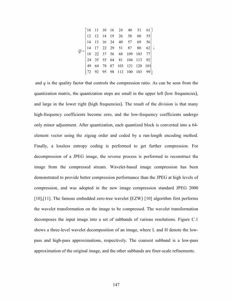
147

=

9910310011298959272

10112012110387786449

921131048164553524

771031096856372218

6280875129221714

5669574024161314

5560582619141212

6151402416101116

Q;

and q is the quality factor that controls the compression ratio. As can be seen from the

quantization matrix, the quantization steps are small in the upper left (low frequencies),

and large in the lower right (high frequencies). The result of the division is that many

high-frequency coefficients become zero, and the low-frequency coefficients undergo

only minor adjustment. After quantization, each quantized block is converted into a 64-

element vector using the zigzag order and coded by a run-length encoding method.

Finally, a lossless entropy coding is performed to get further compression. For

decompression of a JPEG image, the reverse process is performed to reconstruct the

image from the compressed stream. Wavelet-based image compression has been

demonstrated to provide better compression performance than the JPEG at high levels of

compression, and was adopted in the new image compression standard JPEG 2000

[10],[11]. The famous embedded zero-tree wavelet (EZW) [10] algorithm first performs

the wavelet transformation on the image to be compressed. The wavelet transformation

decomposes the input image into a set of subbands of various resolutions. Figure C.1

shows a three-level wavelet decomposition of an image, where L and H denote the low-

pass and high-pass approximations, respectively. The coarsest subband is a low-pass

approximation of the original image, and the other subbands are finer-scale refinements.

148

Figure C.1 Three-level wavelet decomposition

The EZW then scans wavelet coefficients subband by subband, and calculates the zero

trees by marking the coefficients appropriately according to their significance with

respect to a given threshold. The zero tree is an efficient method to represent the wavelet

structure and to quantize wavelet coefficients by discarding the coefficients of the same

orientation and same spatial location at finer scales. Arithmetic coding is finally used to

entropy code the quantized coefficients. Due to the multi-resolution nature of wavelet

decomposition, higher compression ratio can be achieved and more high frequency

components can be saved. Despite its differences from JPEG, EZW nonetheless is based

on the same principle of discarding the high-frequency coefficients.

From the above review, we can see that the standard compression algorithms were

developed for visualization, so they always preserve low frequency and discard high-

frequency coefficients. When applied to compress images for PR, they are not optimal in

terms of the achievable compression ratio and recognition performance, because for PR

high frequencies play a much more important role in discrimination than low frequencies.

Edge enhancement (removing low frequencies) has been proven to be very effective in

improving a PR system’s discrimination capability. Therefore, if we eliminate low-

149

frequency components during compression, it will have several benefits. First, it can

enhance the discrimination performance important for pattern recognition. Second, it

makes it possible to integrate edge enhancement and denoising into the same

compression process and thus reduce computational complexity. Finally, it can increase

the compression ratio significantly. This is because the magnitudes of low-frequency

coefficients tend to be much larger than that of high-frequency, and we only need to

encode middle-to-high frequency coefficients of relatively small magnitude.

C.2 Distortion Criterion for Compressing Images in PR

Let ),( yxr denote the target image and ),( yxs be the observed input scene that

contains the reference image ),( yxr and additive input noise ),( yxn . When the target is

located at unknown coordinates ),( 00 yx , the input scene can be written as

),(),(),( 00 yxnyyxxryxs +−−= , (C.2)

The noise ),( yxn is assumed to be zero-mean additive Gaussian noise. Let ),( yxh be

the recognition FIR filter being used. The resulting output ),( yxc is given by

.),(),(),( ∫∫ ++= dmdnynxmhnmsyxc (C.3)

In particular, ),( yxh is the MSF when ),(),( yxryxh = and is optimal in the sense of

producing the maximum output SNR:

0

2),(

N

dudvvuRSNR

∫∫= ,

where 0N is the noise spectral density, ),( vuR is the Fourier transform of ),( yxr , and

u and v are frequencies respectively along the x axis and y axis. If ),(),( yxryxh = , (C.3)

gives the correlation-based pattern recognition (CRP). CPR has been extensively

150

investigated due to its several advantages over other pattern recognition methods, which

include fast optical implementation, shift invariance, relative senor independence, and no

need of target segmentation. Therefore, as the benchmark, in the simulations, CPR is

used as the optimal pattern recognition method. Usually, correlators must be able not

only to identify the objects in an input image but also to locate the desired target in the

input scene. Ideally, ),( yxc should have a large peak located at ),(),( 00 yxyx = and small

values elsewhere. However, the noise in the input scene can obscure the peak and/or shift

it from its nominal position. According to the theory of parameter estimation, the shifted

coordinates, denoted by ( )00ˆ,ˆ yx , can by estimated using maximum a posteriori (MAP)

estimate,

,)),(ln(),(),(maxarg)ˆ,ˆ( 00000

),(00

00

yxpNdxdyyyxxryxsyxyx

+−−= ∫∫ (C.4)

where ),( 00 yxp is the coordinate a priori distribution density. This is because the estimate

having the minimum probability of error is the one that has maximum a posteriori

probability that the coordinate has a particular value given the input signal ),( yxs . It can

be proven that the Cramer Rao Lower Bound on the variances of the location errors in

−x and −y directions are given by [54]

∫∫

×≥

dudvvuRu

Ncxx 222

02

),(4πσ , (C.5)

∫∫

×≥

dudvvuRv

Ncyy 222

02

),(4πσ . (C.6)

where ),( vuR is the Fourier transform of ),( yxr , and u and v are the frequencies along

the −x axis and −y axis. xc and yc are some constants. This view drives us to choose the 2-

151

D DFT as our transform to allow discarding less useful frequency components and guide

the quantization of the rest of coefficients. Using the 2-D discrete Fourier transform on

(C.2) and using similar procedures as in Section 3.1, the Fisher information for the

location estimation in −x and −y directions are

∑∑−

=

−

=

=1

0

1

0 0

22

2

2 ),(20

M

v

N

u

xN

vuRu

MJ

π, (C.7)

∑∑−

=

−

=

=1

0

1

0 0

22

2

2 ),(20

M

v

N

u

yN

vuRv

NJ

π, (C.8)

where ),( vuR is the Fourier transform of ),( yxs , whose size is NM × , and ),(2 vuq is

the variance of the quantization noise on the Fourier coefficient at ),( vu . From (C.7) and

(C.8), we can see that the accuracy of locating the reference image in the received image

depends more on the high frequency components than low frequency components, It also

can be seen from (C.7) and (C.8) that the high frequency coefficients in ),( vuR should

be weighted more heavily than the low frequency coefficients. This implies that high

frequency components play a more important role than low frequency components in PR.

So for compressing images for PR, more weight should be given to the important high

frequency components instead of to the low frequencies.

Since maximizing 0x

J and 0y

J can achieve improved location accuracy in pattern

recognition, (C.7) and (C.8) can be used as criteria for image compression in CPR.

Applying the approximate model in Chapter 3, if we replace ),( vuR with ),( vuS , and

treat the x and y directions equally important, we can add 2xF and

2yF to form a single

tractable and data centric distortion measure,

152

( )∑∑−

=

−

= +

+=

+=

1

0

1

02

0

222222

2

),(

/),(/),(2

)(ˆ)(ˆ)(ˆ00

M

v

N

u

xx

vuqN

NvuSvMvuSu

sJsJsJ

π. (C.9)

We can use the same numerical optimization method as in Chapter 3 to design an optimal

transform coder according to (C.9) under the bit constraint R. However, here we simply

modify the standard compression algorithms to reflect this criterion so they can be more

suitable for image PR. For example, for JPEG compression, we only change their

quantization step and leave the other processing steps untouched. The advantage of doing

such is that we are still able to use the standard decoders to decompress the images

compressed by the proposed algorithms.

C.3 Modifying the Standard Compression Algorithms for CPR

We first modify the JPEG so it can be more suitable for CPR. The DCT is closely

related to the discrete Fourier transform (DFT). Actually, DCT coefficients qy of any m-

point sequence x are related to the m2 -point DFT coefficients qy( of the symmetrically

extended sequence, x(, by a constant scale factor, which is signal dependent; i.e.,

q

qm

j

qq yem

cy(

=

−2

2

π

, 1,,1,0 −= mq L . (C.10)

where mcq /1= when 0=q , and mcq /2= otherwise.

The numerator of the summation (C.7) and (C.8) can be approximated by

∑∑−

=

−

=

+1

0

1

0

222 )(M

j

N

i

ijTji , (C.11)

for each of the 8×8 DCT blocks within a scaling factor that has no effect on the

compression. For the criterion obtained in Section C.2, we know that high-frequency

153

DCT coefficients should be weighted and retained with refined quantization, whereas

low-frequency DCT coefficients should be discarded or quantized coarsely. This can be

done by carefully selecting a quantization array. For simplicity, we rotate the JPEG’s

quantization matrix by 180 deg and use it as our quantization matrix:

=

1611101624405161

1212141926586055

1413162440576956

1417222951878062

182237566810910377

243555648110411392

49647887103121120101

7292959811210010399

*Q

This rotated matrix can perform fine quantization for high frequency DCT coefficients

and coarse quantization for low-frequency DCT coefficients, because the quantization

steps are small at the lower right and large at the upper left corner. Thus the modified

JPEG for CPR involves the following steps. After DCT transformation, each DCT block

is weighted by a weight matrix and then quantized using the 180-deg-rotated quantization

matrix Q*. That is, (C.11) is modified as

maskQq

WTroundT

ij

ijij

ij ×

⋅

×=

*ˆ , (C.12)

where jiW , are the components of the weight matrix and should be ( )22 ji + according

to (C.12). Considering that the quantized coefficients are scanned in a zigzag order, the

coding can also be simplified by changing the weight matrix to the 8×8 zigzag index

matrix

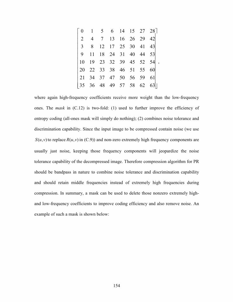
154

6362585749483635

6159565047373421

6055514638332220

5452453932231910

534440312418119

43413025171283

4229261613742

282715146510

,

where again high-frequency coefficients receive more weight than the low-frequency

ones. The mask in (C.12) is two-fold: (1) used to further improve the efficiency of

entropy coding (all-ones mask will simply do nothing); (2) combines noise tolerance and

discrimination capability. Since the input image to be compressed contain noise (we use

),( vuS to replace ),( vuR in (C.9)) and non-zero extremely high frequency components are

usually just noise, keeping those frequency components will jeopardize the noise

tolerance capability of the decompressed image. Therefore compression algorithm for PR

should be bandpass in nature to combine noise tolerance and discrimination capability

and should retain middle frequencies instead of extremely high frequencies during

compression. In summary, a mask can be used to delete those nonzero extremely high-

and low-frequency coefficients to improve coding efficiency and also remove noise. An

example of such a mask is shown below:

155

00000011

00000111

00001111

00011110

00111100

00111000

01110000

11000000

,

where only coefficients of middle frequencies from 16 to 39 are encoded. The mask

could be determined either by optimizing some measure or by extensive experimentation.

The latter was used in this paper.

In the final stage of compression, the obtained quantized coefficients from (C. 11) are

entropy-encoded. Since only middle-frequency (and some high-frequency) components

are coded and they have much smaller magnitudes than low-frequency components, a

higher compression ratio than the standard JPEG can be obtained. Although multiplying

DCT coefficients with a weight matrix will increase the magnitudes of the quantized

coefficients, this can be alleviated by increasing the corresponding quality factor. It is to

be noted that the quality of an image in PR has a different meaning from the quality in

human visualization. Therefore, the quality factors (C.12) and (C.2) are not the same.

We can modify the wavelet-based image compression algorithms as well for PR in a

similar way by emphasizing middle- to high-frequency components. The wavelet-based

algorithms are based on the multiresolution decomposition of the image to be compressed.

For visualization, the LL (low-frequency) band at the highest level is considered as most

important, and the other bands, containing edge information, are classified as of minor

importance, with the degree of importance decreasing from the top of the pyramid to the

156

bands at the bottom. As a result, a large number of bits are assigned to encode the LL

band, and many coefficients at higher-frequency subbands (finer resolutions) are

discarded. However, for pattern recognition, we know that edge information is more

important. Accordingly, we suggest encoding the LH and HL bands and discarding the

LL and HH bands. In this way, a much higher compression ratio can be obtained while

simultaneously enhancing the discrimination performance. Wavelet denoising [7] can be

applied to the wavelet coefficients to remove possible noise in the encoding process.

C.4 Simulation Results

Computer simulations were performed to test the performance of the proposed

algorithms. The input image used is an infrared image as shown in Fig. C.2, and the truck

located at the left is used as the reference image. We compare the performance of the

standard JPEG, the standard EZW, and the proposed modified JPEG and EZW. The input

image is compressed using these four compression methods respectively, and then

reconstructed and cross-correlated with the reference image. Figure C.3(a), C.3(b), C.3(c),

and C.3(d) show, respectively, the reconstructed images from the standard JPEG (or

EZW); the modified JPEG with q=1, weight matrix 22 ji + , an all-ones mask; the

modified JPEG with q=1, the zigzag weight matrix, and the example mask; and the

modified EZW algorithms. It is seen that the reconstructed image from the standard JPEG

or EZW is almost identical to the original image, while in the reconstructed images from

the modified algorithms, the middle and high frequency components are emphasized.

Figure C.3(b), C.3(c), and C.3(d) will not be acceptable for visualization purposes, but

they are good for pattern recognition. This can be seen from the normalized correlation

results as shown in Figure C.4. Figure C.4(a) is the normalized correlation output with

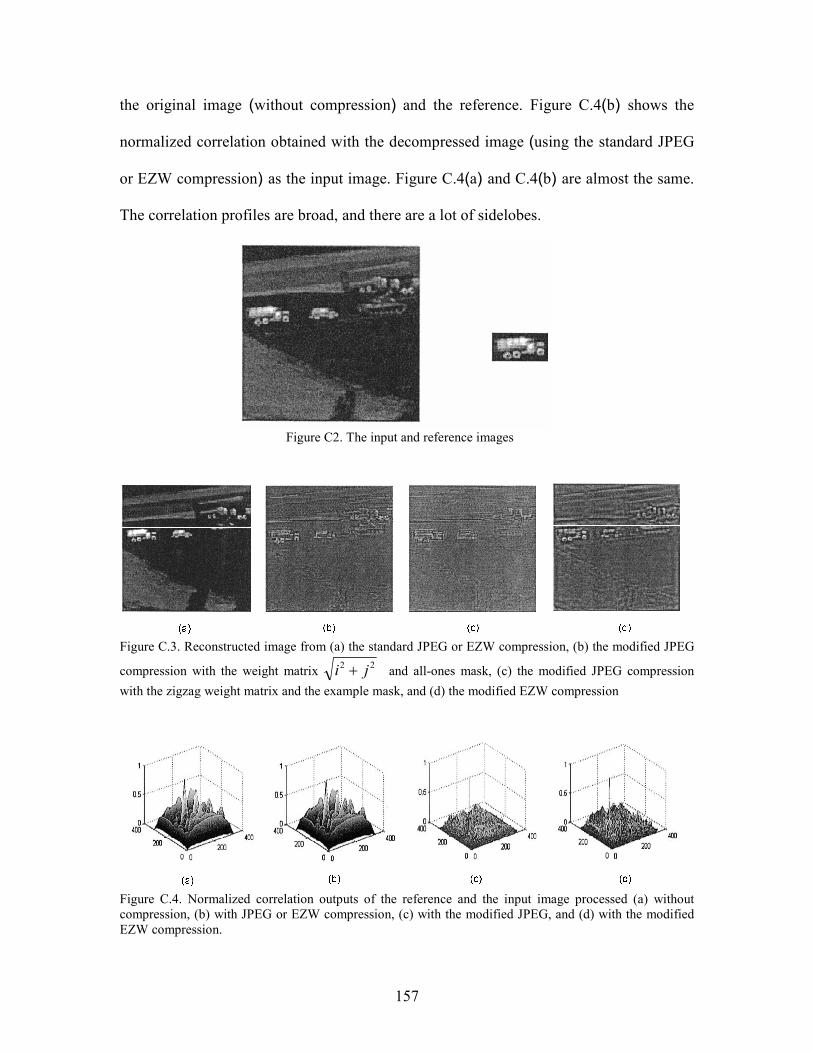
157

the original image (without compression) and the reference. Figure C.4(b) shows the

normalized correlation obtained with the decompressed image (using the standard JPEG

or EZW compression) as the input image. Figure C.4(a) and C.4(b) are almost the same.

The correlation profiles are broad, and there are a lot of sidelobes.

Figure C2. The input and reference images

Figure C.3. Reconstructed image from (a) the standard JPEG or EZW compression, (b) the modified JPEG

compression with the weight matrix 22 ji + and all-ones mask, (c) the modified JPEG compression

with the zigzag weight matrix and the example mask, and (d) the modified EZW compression

Figure C.4. Normalized correlation outputs of the reference and the input image processed (a) without

compression, (b) with JPEG or EZW compression, (c) with the modified JPEG, and (d) with the modified

EZW compression.

158

However, with the proposed modified JPEG and EZW compression, we can obtain a

much sharper correlation peak, as shown in Figure C.4(c) and C.4(d), respectively. For

the compression ratio, the standard JPEG baseline and the modified JPEG with the zigzag

weight matrix are 30:1 and 73.5:1, respectively whereas the standard EZW and the

modified EZW have compression ratios of 533:1 and 624:1, respectively.

Figure C.5: Compression ratio versus quality factor

The compression ratio of the modified JPEG algorithm depends on the quality factor,

the weight matrix, and the shape of the mask. Figure C.5 illustrates the relationship

between q-factor and compression ratio when the zigzag weight matrix and the example

mask shown in C.3 are used. Figures C.6 and C.7 show the reconstructed images and

correlation distributions using the modified JPEG when the quality factor is 12

(compression ratio 117:1) and 35 (compression ratio 820:1), respectively. It is seen that

we can still get sharp correlation peaks at high compression ratio. The quality of the

decompressed image is degraded significantly as the compression ratio increases. The

edges of the two other smaller vehicles (car and tank) are almost lost in Figure C.7 due to

the extremely high compression ratio. Low contrast and small spatial support are other

159

reasons for losing edges. No compression method can be guaranteed to work for all

objects with a high compression ratio.

Figure C.6: Reconstructed image and correlation output when q=12.

Figure C.7: Reconstructed image and correlation output when q=35.

Next, white Gaussian noise was added to the input image as shown in Figure C.8 (a)

to test the noise performance of the proposed methods. The noise has zero mean and a

standard deviation of 20. The normalized correlation distributions of the reference and

the noisy input processed with the modified JPEG (with q=12) and the modified EZW,

are obtained as shown in Figure C.8 (b) and C.8 (c), respectively. It is seen that they can

tolerate additive noise. When the noise becomes heavy, the performance of the modified

JPEG degrades faster than that of the modified EZW. From the results obtained, the

modified EZW has the best performance, considering the compression ratio, correlation

output, and noise tolerance. This is partially because the modified EZW has better

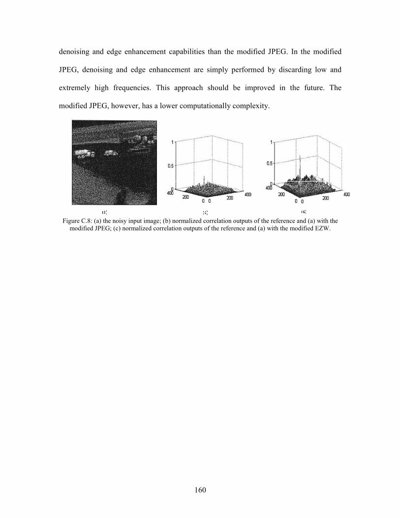
160

denoising and edge enhancement capabilities than the modified JPEG. In the modified

JPEG, denoising and edge enhancement are simply performed by discarding low and

extremely high frequencies. This approach should be improved in the future. The

modified JPEG, however, has a lower computationally complexity.

Figure C.8: (a) the noisy input image; (b) normalized correlation outputs of the reference and (a) with the

modified JPEG; (c) normalized correlation outputs of the reference and (a) with the modified EZW.

161

APPENDIX D

Symmetric Indexing

In the examples in Sections IV-A and IV-B we used a symmetric indexing of the data

of which we assess the Fisher information: for TDOA estimation we symmetrically index

the DFT coefficients in (3.26) and for FDOA estimation we symmetrically index the

samples in (3.33). Why do we choose these seemingly arbitrary indexing schemes?

Fundamentally, the choice of which sample or DFT coefficient we index as zero is an

arbitrary one that arises in the mathematical analysis; thus, such an arbitrary naming

should have no effect on the amount of Fisher information is available in from the data.

However, for some problems the choice of the data indexing can influence the form of

the Fisher information. For example, in the FDOA problem, if instead of the indexing

used in (3.33) we changed the indexing of the signal samples to

2/,,1,,1,,2/][][][

2/,,1,,1,,2/][][][

2

)2/(

2

1

)2/(

1

0

0

NnnnnNnnnwensnx

NnnnnNnnnwensnx

ooooo

vj

ooooo

vj

++−−=+=

++−−=+=

−

+

KK

KK

ν

ν

(D.1)

then the total Fisher information can be made arbitrarily large by increasing the value of

|no|. This motivates choosing the smallest possible value of |no|, or no = 0. In other words,

the indexing should be symmetric in the TDOA and FDOA problems. In other problems

similar attention should be paid to the impact of the indexing on the Fisher information.

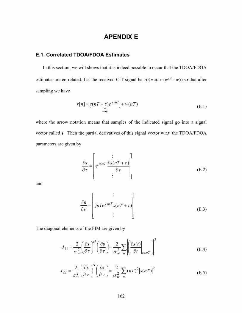
162

APENDIX E

E.1. Correlated TDOA/FDOA Estimates

In this section, we will shows that it is indeed possible to occur that the TDOA/FDOA

estimates are correlated. Let the received C-T signal be )()()( twetstrtj ++= ντ so that after

sampling we have

)()(][ nTwenTsnrnTj ++=

→44 344 21

s

ντ (E.1)

where the arrow notation means that samples of the indicated signal go into a signal

vector called s. Then the partial derivatives of this signal vector w.r.t. the TDOA/FDOA

parameters are given by

∂+∂

=∂∂

M

M

ττ

τν )(nTs

enTjs

(E.2)

and

+=∂∂

M

M

)( τν

νnTsjnTe

nTjs

(E.3)

The diagonal elements of the FIM are given by

∑

∂∂

=

∂∂

∂∂

==n nTtw

H

wt

tsJ

2

2211

)(22

σττσ

ss

(E.4)

∑=

∂∂

∂∂

=nw

H

w

nTsnTJ22

2222 )()(22

σννσ

ss

(E.5)

163

The off-diagonal elements of the FIM are given by

∂+∂

+−=

∂∂

∂∂

= ∑nw

H

w

nTsnTjnTsJ

ττ

τστνσ

)()(Re

2Re

2 *

2212ss

(E.6)

with J21 = J12. Let the signal be a general complex equivalent lowpass signal; then it has

the general form of

)()()( τφττ ++=+ nTjenTAnTs (E.7)

so that we get

)()()(

)()()(

)(

)()(

τφτ

τττ

τττ

ττ

τ

τφ

τφτφ

+∂∂

+++∂∂

=

∂∂

+++∂∂

=+∂∂

+

++

nTnTjsnTAe

enTAnTAenTs

nTj

nTjnTj

(E.8)

Now using (E.8) in (E.6) gives

∑∑

∑

+∂∂

++

+

∂∂

+−=

+∂∂

+++∂∂

+−=

+

+

nwn

nTj

w

n

nTj

w

nTnTsnTnTAenTjnTs

nTnTjsnTAenTjnTsJ

)()(2

)()(Re2

)()()()(Re2

2

2

)(*

2

)(*

212

τφτ

τσ

ττ

τσ

τφτ

τττ

τσ

τφ

τφ

(E.9)

Now clearly this doesn’t go to zero in general, although there may be some special

cases [86].

E.2. FIM for TDOA/FDOA of a Chirp Signal

Let the signal be a complex linear chirp signal given by

2)2/()( tjjeets

αφ= (E.10)

so that we get

164

)()(2))(2/(

nTnTsjenTejnTsnTjj αα αφ ==& (E.11)

Now using (E.11) in (E.4)-(E6) gives

( )

( ) ∑∑

∑∑

∑∑∑

=

−=

==

===

nn

nn

nn

nTjj

n

nTnTnTsjnTjnTsJ

nTnTsnTJ

nTenTejnTsJ

22*

2222

222

))(2/(2

2)()(Re2

2)()(2

)(22)(22

αα

αα

ντ

νν

αφττ &

(E.12)

or in matrix form

= ∑

1

2

222

α

αα

n

nTJ . (E.13)

In the following simulation of testing if we could apply equations (4.30), (4.31) and

(4.37) by using PR filter bank and the short-time Fourier transform (STFT) to

numerically compute the FIM elements and then compare the result to the analytically

derived theoretical result for the linear chirp signal. Because vvJ in (E.12) is a constant

with respect to the sweep rate of the chirp signalα , so α, so we can look at the other

terms relative to this term: J11 / J22 = α2 and J12 / J22 = α. Plots of the numerical and

theoretical results for the case of using a complex filter bank and STFT are shown in

Figure E.1 and Figure E.2 respectively.

165

-2 -1.5 -1 -0.5 0 0.5 1 1.5 2

x 10-3

5.2

5.4

5.6

5.8

6

6.2

6.4x 10

9

α

J22

-2 -1.5 -1 -0.5 0 0.5 1 1.5 2

x 10-3

0

0.5

1

1.5

2

2.5

3x 10

-6

-2 -1.5 -1 -0.5 0 0.5 1 1.5 2

x 10-3

-2

-1

0

1

2x 10

-3

Numerical

Theoretical

α

α

J11/J22

J12/J22

Figure E.1: Quality of numerical evaluation of FIM via complex filter bank

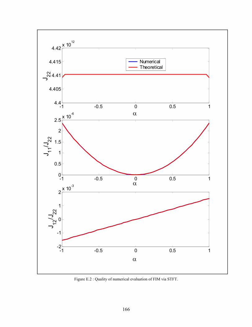
166

-1 -0.5 0 0.5 14.4

4.405

4.41

4.415

4.42x 10

12

α

J22

-1 -0.5 0 0.5 10

0.5

1

1.5

2

2.5x 10

-6

-1 -0.5 0 0.5 1-2

-1

0

1

2x 10

-3

Numerical

Theoretical

α

α

J11/J22

J12/J22

Figure E.2 : Quality of numerical evaluation of FIM via STFT.

167

Appendix F:

Complex PR Filter Banks

A. Introduction

Let g0[n] , g1[n], h0[n], h1[n] be a set of N-order FIR filters that lead to a perfect

reconstruction (PR) filter bank arising from a tree cascade structure; the gi[n] are the analysis

filters and the hi[n] are the synthesis filters. For this analysis we will assume a “full tree”

decomposition; a four-channel example of the analysis bank is shown in Figure F.1 and the

corresponding synthesis bank is shown in Figure F.2.

In this example we have assumed that the analysis filters g0[n] and g1[n] are chosen to be

half-band lowpass and half-band highpass, respectively, as is typical and virtually universal in the

literature. As a result of this choice, note that the channel frequency responses shown in Figure

F.1 are “two sided,” in that each channel passes both positive and negative frequencies.

In many applications it is desirable to have so-called one-sided channels. Although there are

known methods for the direct design and implementation of such filters (e.g., DFT-based filter

banks and polyphase filter banks), tree-based methods for one-sided filter banks seem to be

relatively unknown. Because there are times when a tree-based approach is desirable for one-

sided filter banks it is worthwhile to address a simple trick that allows conversion of any two-

sided tree-based PR filter bank into a one-sided tree-based PR. This then brings to bear on the

one-sided problem a huge body of literature devoted to the two-sided problem.

B. Channel Response Analysis for Two-Sided Filter Banks

To aid our later analysis we will analyze this 4-channel filter bank to verify that it provides

the kind of channel responses shown in Figure F.1. The easiest way to do this is to use the

decimation identity to move the “inside” decimators to the output side, then find the four

channel’s outputs before decimation, then impart the effect of the 4x decimation. The decimation

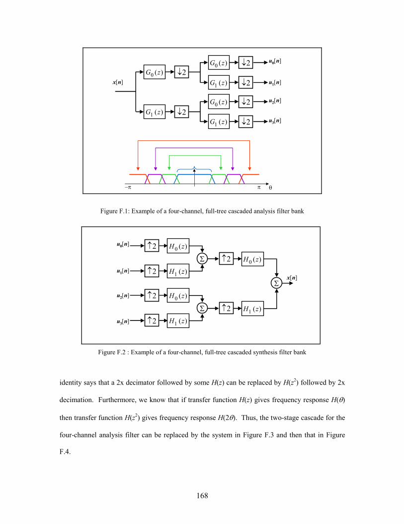
168

26/27

↓2)(0 zG

↓2)(1 zG

↓2)(0 zG

↓2)(1 zG

u0[n]

u1[n]

u2[n]

u3[n]

x[n]

π θ–π

↓2)(0 zG

↓2)(1 zG

Figure F.1: Example of a four-channel, full-tree cascaded analysis filter bank

↑2

↑2

↑2

u0[n]

u1[n]

u2[n]

u3[n]

x[n]

)(0 zH

)(1 zH

Σ

↑2

↑2

↑2

)(0 zH

)(1 zH

Σ

)(0 zH

)(1 zH

Σ

Figure F.2 : Example of a four-channel, full-tree cascaded synthesis filter bank

identity says that a 2x decimator followed by some H(z) can be replaced by H(z2) followed by 2x

decimation. Furthermore, we know that if transfer function H(z) gives frequency response H(θ)

then transfer function H(z2) gives frequency response H(2θ). Thus, the two-stage cascade for the

four-channel analysis filter can be replaced by the system in Figure F.3 and then that in Figure

F.4.

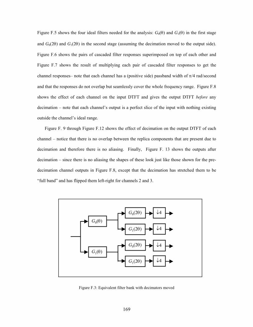
169

Figure F.5 shows the four ideal filters needed for the analysis: G0(θ) and G1(θ) in the first stage

and G0(2θ) and G1(2θ) in the second stage (assuming the decimation moved to the output side).

Figure F.6 shows the pairs of cascaded filter responses superimposed on top of each other and

Figure F.7 shows the result of multiplying each pair of cascaded filter responses to get the

channel responses– note that each channel has a (positive side) passband width of π/4 rad/second

and that the responses do not overlap but seamlessly cover the whole frequency range. Figure F.8

shows the effect of each channel on the input DTFT and gives the output DTFT before any

decimation – note that each channel’s output is a perfect slice of the input with nothing existing

outside the channel’s ideal range.

Figure F. 9 through Figure F.12 shows the effect of decimation on the output DTFT of each

channel – notice that there is no overlap between the replica components that are present due to

decimation and therefore there is no aliasing. Finally, Figure F. 13 shows the outputs after

decimation – since there is no aliasing the shapes of these look just like those shown for the pre-

decimation channel outputs in Figure F.8, except that the decimation has stretched them to be

“full band” and has flipped them left-right for channels 2 and 3.

G0(θ)

G1(θ)

G0(2θ)

G1(2θ)

G0(2θ)

G1(2θ)

↓4

↓4

↓4

↓4

Figure F.3: Equivalent filter bank with decimators moved

170

G0(θ) G0(2θ) ↓4

↓4

↓4

↓4

G0(θ) G1(2θ)

G1(θ) G0(2θ)

G1(θ) G1(2θ)

Figure F. 4: Equivalent filter bank with decimators moved and blocks combined

π 2π 3π 4π–π–2π–3π–4π θ

G0(θ)

π 2π 3π 4π–π–2π–3π–4π θ

G1(θ)

π 2π 3π 4π–π–2π–3π–4π θ

G0(2θ)

π 2π 3π 4π–π–2π–3π–4π θ

G1(2θ)

Figure F. 5: Ideal filters for the various stages (w/ decimation moved to end)

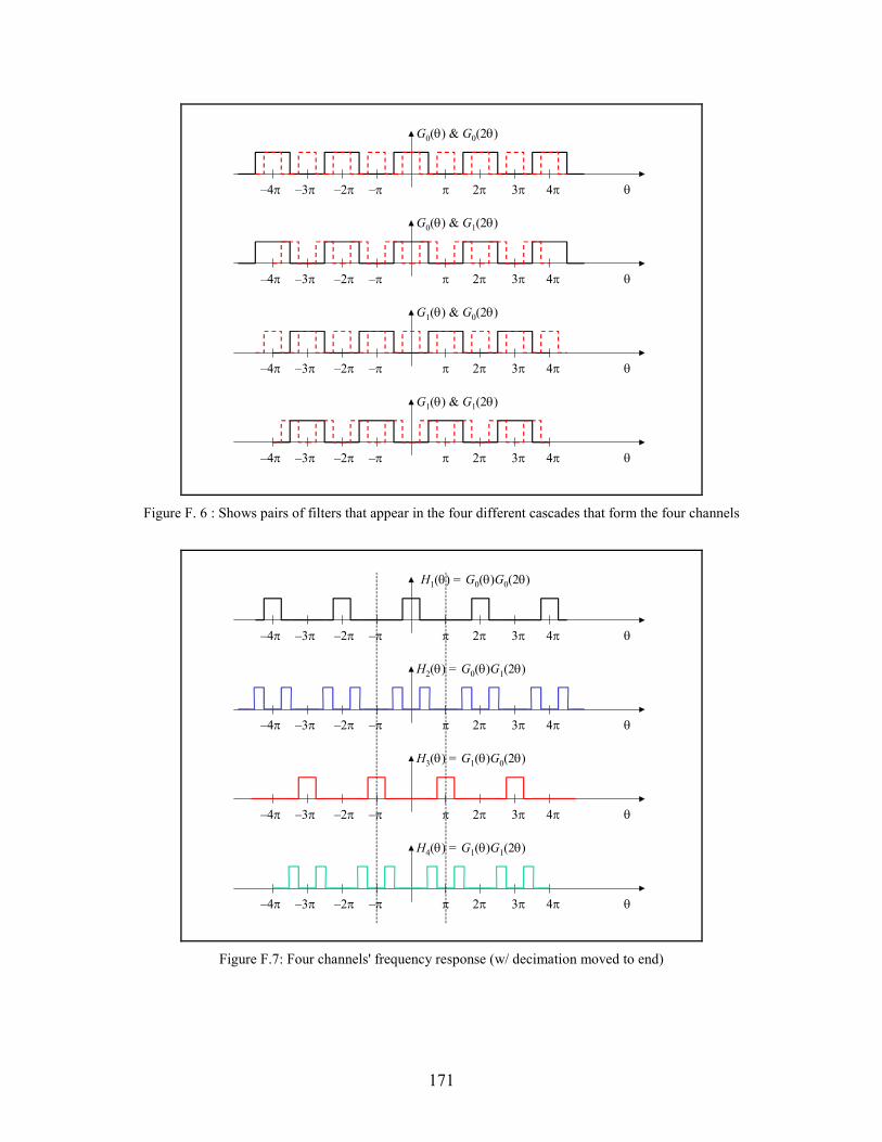
171

π 2π 3π 4π–π–2π–3π–4π θ

G0(θ) & G0(2θ)

π 2π 3π 4π–π–2π–3π–4π θ

G0(θ) & G1(2θ)

π 2π 3π 4π–π–2π–3π–4π θ

G1(θ) & G0(2θ)

π 2π 3π 4π–π–2π–3π–4π θ

G1(θ) & G1(2θ)

Figure F. 6 : Shows pairs of filters that appear in the four different cascades that form the four channels

π 2π 3π 4π–π–2π–3π–4π θ

H1(θ) = G0(θ)G0(2θ)

π 2π 3π 4π–π–2π–3π–4π θ

H2(θ) = G0(θ)G1(2θ)

π 2π 3π 4π–π–2π–3π–4π θ

H3(θ) = G1(θ)G0(2θ)

π 2π 3π 4π–π–2π–3π–4π θ

H4(θ) = G1(θ)G1(2θ)

Figure F.7: Four channels' frequency response (w/ decimation moved to end)

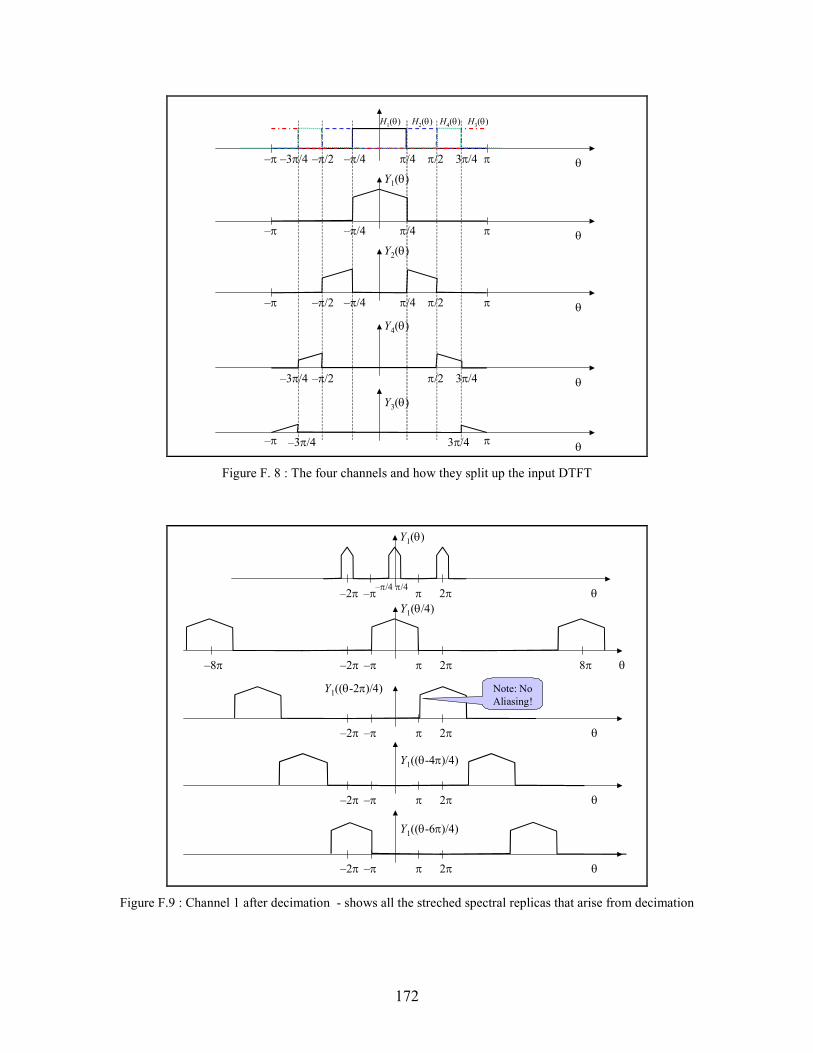
172

π–π θ

θ

Y1(θ)

π/4 π/2 3π/4–π/4–3π/4 –π/2

π–π π/4–π/4

θπ–π π/4 π/2–π/4–π/2

Y2(θ)

H1(θ) H2(θ) H4(θ) H3(θ)

θ

Y4(θ)

θ

Y3(θ)

π/2 3π/4–3π/4 –π/2

3π/4–3π/4 π–π

Figure F. 8 : The four channels and how they split up the input DTFT

θ

Y1(θ)

π–ππ/4–π/4

2π–2π

θ

Y1(θ/4)

π–π 2π–2π

θ

Y1((θ-2π)/4)

π–π 2π–2π

8π–8π

θ

Y1((θ-4π)/4)

π–π 2π–2π

Note: No

Aliasing!

θ

Y1((θ-6π)/4)

π–π 2π–2π

Figure F.9 : Channel 1 after decimation - shows all the streched spectral replicas that arise from decimation

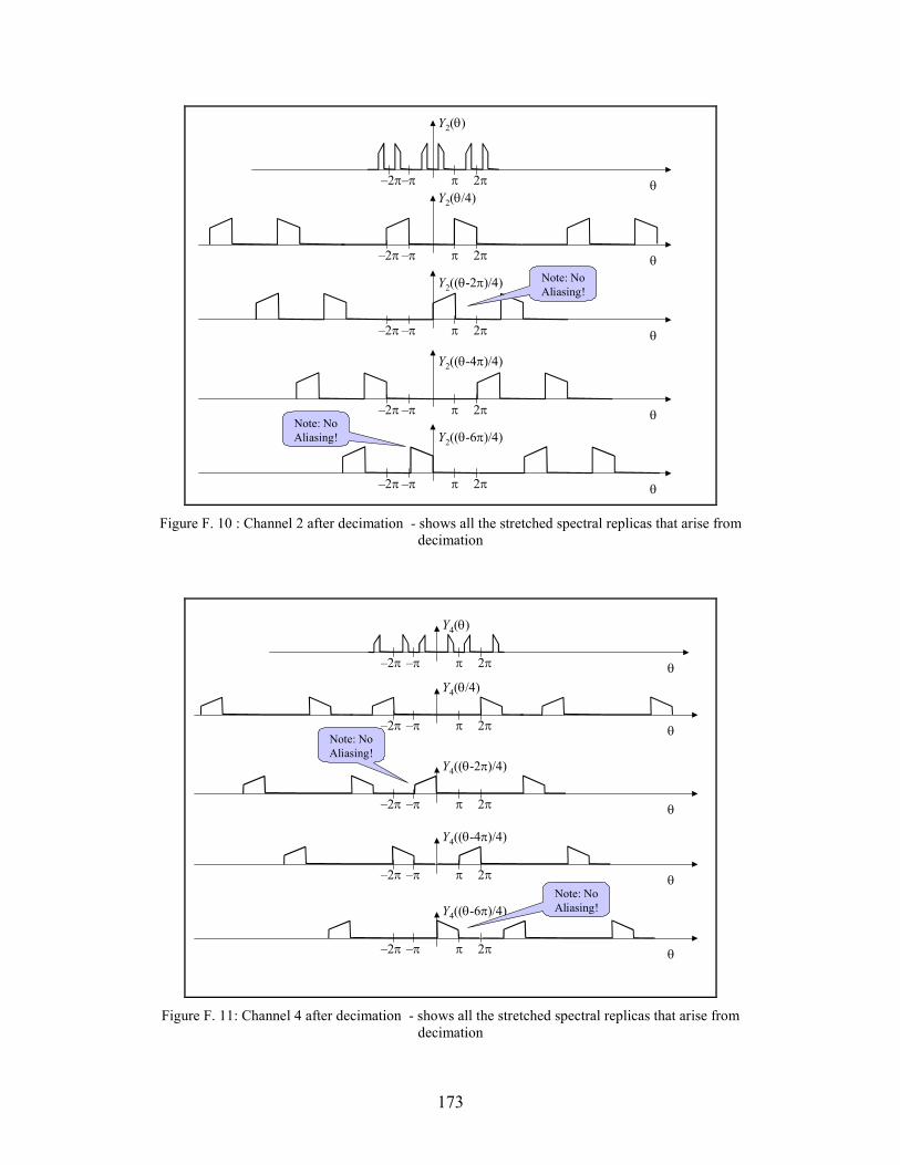
173

θπ–π

Y2(θ)

2π–2π

θπ–π

Y2(θ/4)

2π–2π

θπ–π

Y2((θ-2π)/4)

2π–2π

θπ–π

Y2((θ-4π)/4)

2π–2π

θπ–π

Y2((θ-6π)/4)

2π–2π

Note: No

Aliasing!

Note: No

Aliasing!

Figure F. 10 : Channel 2 after decimation - shows all the stretched spectral replicas that arise from

decimation

θ

Y4(θ)

π–π 2π–2π

θ

Y4(θ/4)

π–π 2π–2π

θ

Y4((θ-2π)/4)

π–π 2π–2π

θ

Y4((θ-4π)/4)

π–π 2π–2π

θ

Y4((θ-6π)/4)

π–π 2π–2π

Note: No

Aliasing!

Note: No

Aliasing!

Figure F. 11: Channel 4 after decimation - shows all the stretched spectral replicas that arise from

decimation

174

θ

Y3(θ)

π–π 2π–2π

θ

Y3(θ/4)

π–π 2π–2π 4π–4π

θ

Y3((θ-2π)/4)


θ

Y3((θ-4π)/4)


θ

Y3((θ-6π)/4)


Note: No

Aliasing!

Note: No

Aliasing!

Figure F. 12: Channel 3 after decimation - shows all the stretched spectral replicas that arise from

decimation

Y1_dec(θ)

π–π θ

Y2_dec(θ)

π–π θ

Y4_dec(θ)

π–π θ

Y3_dec(θ)

π–π θ

Figure F.13: Channel output DTFT’s after decimation - only shows standard –π to π range

175

C. Background: Standard Conditions For PR

First some preliminaries on the conditions used to achieve PR in the two-sided filter banks.

The order N of the FIR filters must be odd (and therefore the length L = N+1 is even).

Cancellation of aliasing is ensured when the synthesis filters are related to the analysis filters

according to

)()(

)()(

01

10

zGzH

zGzH

−−=

−=

(F.1)

which in the time domain becomes

Nnngnh

Nnngnh

n

n

,,2,1,0],[)1(][

,,2,1,0],[)1(][

01

10

K

K

=−−=

=−=

(F.2)

With aliasing cancelled through this relationship between the synthesis filters and the analysis

filters, the transfer function from input on the analysis side to the output on the synthesis side

becomes

)()()()()( 1010 zGzGzGzGzT −−−= . (F.3)

The following relationship between the two analysis filters is imposed to help enforce the PR

condition:

)()()( 101

−− −−= zGzzG N (F.4)

which in the time domain is equivalent to

NnnNgng n ,,2,1,0],[)1(][ 01 K=−−= (F.5)

which turns (F.2) into

Nnngnh

NnnNgnh

n ,,2,1,0],[)1(][

,,2,1,0],[][

01

00

K

K

=−−=

=−=

(F.6)

176

Substitution of (F.4) into (F.3) leads to

)]()()()([)( 100

100

−−− −−−= zGzGzGzGzzT N. (F.7)

and thus a sufficient condition for perfect reconstruction is

1)()(2

0

2

0 =−+ πθθ GG , (F.8)

where )(0 θG is the frequency response of the filter; in the time domain this condition is

equivalent to

][]2[],[ 00 kkngng δ=+ , (F.9)

which means that the filter g0[n] is orthogonal to its even-integer translates. Thus, a set of filters

designed to satisfy (F.5)–(F.9) will lead to a two-sided PR filter bank. The typical approach is to

design a half-band lowpass filter g0[n] that satisfies (F.8) and (F.9) and then determine the other

three filters from (F.5) and (F.6). The relationships in (F.5) and (F.6) constitute a strict linkage

between the four filters in the filter banks. The equations given in (F.5) and (F.6) show how to

get the other three filters once you have g0[n]; similarly, given any one of the four filters it is

possible to get the other three using similar relationships; these relationships are summarized in

Figure F.14, where the solid line connections correspond to (F.5) and (F.6) and the dashed line

connections can be derived from them.

When the filter g0[n] is chosen to be a half-band lowpass filter, then g1[n] will become a half-

band highpass filter, as imposed by (F.5); and it is that structure that leads to the standard two-

sided filter bank. Thus, to get a one-sided filter bank it seems that we may simply need to chose

g0[n] in a slightly different way. As shown in the next subsection, if we first choose g0[n] to be a

complex half-band filter that satisfies (F.8) then we can get the desired complex one-sided filter

bank through a similar set of relationships as (F.5) and (F.6).

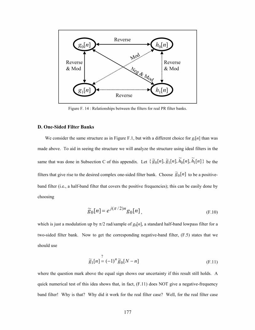
177

g0[n] h0[n]

g1[n] h1[n]

Reverse

Reverse

Reverse

& Mod

Reverse

& Mod

Mod

Neg & Mod

Figure F. 14 : Relationships between the filters for real PR filter banks.

D. One-Sided Filter Banks

We consider the same structure as in Figure F.1, but with a different choice for gi[n] than was

made above. To aid in seeing the structure we will analyze the structure using ideal filters in the

same that was done in Subsection C of this appendix. Let ][~

],[~

],[~],[~ 1010 nhnhngng be the

filters that give rise to the desired complex one-sided filter bank. Choose ][~0 ng to be a positive-

band filter (i.e., a half-band filter that covers the positive frequencies); this can be easily done by

choosing

][][~0

)2/(0 ngeng nj π= , (F.10)

which is just a modulation up by π/2 rad/sample of g0[n], a standard half-band lowpass filter for a

two-sided filter bank. Now to get the corresponding negative-band filter, (F.5) states that we

should use

][~)1(][~0

?

1 nNgng n −−= (F.11)

where the question mark above the equal sign shows our uncertainty if this result still holds. A

quick numerical test of this idea shows that, in fact, (F.11) does NOT give a negative-frequency

band filter! Why is that? Why did it work for the real filter case? Well, for the real filter case

178

the time reversal does not change the magnitude of the frequency response and then the

modulation converts this into a highpass filter. However, for a complex filter the time reversal

DOES change the magnitude of the frequency response; it changes it into a negative-band filter!

So maybe we could just do the time reversal of (F.11) to get the desired negative-band filter; but

that would provide us with a theory for the complex case that does NOT naturally degenerate to

the known real-valued theory.

To find the answer we have to look at (F.4), which is the truer starting point than (F.5). The

inverse-z in (F.4) (which is responsible for the time reversal) causes the filter transfer function

zeros to move as show in Figure F.15; for real filters the zeros must appear in conjugate pairs and

they then move into conjugate pairs. Half-band lowpass filters will have zeros along the left-had

side of the unit circle and the inverse-z mapping will keep them on that side; thus, they remain

half-band lowpass filters after time reversal. However, for half-band positive-pass filters a zero

on the negative frequency side of the unit circle will get mapped into the positive frequency side

(which is not what we want). But… conjugating the filter coefficients and doing a time reversal

will leave them on the negative frequency side as shown in Figure F.16. Note that this operation

will naturally degenerate to the known real-valued theory.

Thus, we have demonstrated that a time reversal and coefficient conjugation is the mapping

needed to get the negative-band filter from the positive band filter; thus, (F.11) should be changed

to

][~)1(][~ *01 nNgng n −−= , (F.12)

which now covers the negative frequency band. This is shown in Figure F.17.

If we now walk our way through the equivalent four-channel cascade with the decimators

moved to the end we will see what kind of analysis bank this choice of filters will give. The

plots in Figure F.17 show the interaction between the two filters in each channel. The plots in

Figure F.18 show the frequency response magnitudes for each of the four filter bank channels.

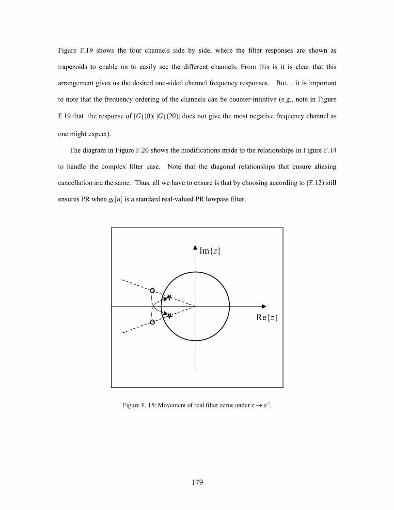
179

Figure F.19 shows the four channels side by side, where the filter responses are shown as

trapezoids to enable on to easily see the different channels. From this is it is clear that this

arrangement gives us the desired one-sided channel frequency responses. But… it is important

to note that the frequency ordering of the channels can be counter-intuitive (e.g., note in Figure

F.19 that the response of |G1(θ)| |G1(2θ)| does not give the most negative frequency channel as

one might expect).

The diagram in Figure F.20 shows the modifications made to the relationships in Figure F.14

to handle the complex filter case. Note that the diagonal relationships that ensure aliasing

cancellation are the same. Thus, all we have to ensure is that by choosing according to (F.12) still

ensures PR when g0[n] is a standard real-valued PR lowpass filter.

Rez

Imz

Figure F. 15: Movement of real filter zeros under z → z-1.

180

Rez

Imz

Figure F.16 : Movement of complex filter zeros under coefficient conjugation and z → z-1; the first move to

the gray star location is due to the z → z-1

and the second move is due to coefficient conjugation.

π 2π 3π 4π–π–2π–3π–4π θ

π 2π 3π 4π–π–2π–3π–4π θ

)(~

0 θG

)(~1 θG

Figure F.16 : Ideal Filters for the first stage of the one-sided filter bank

181

π 2π 3π 4π–π–2π–3π–4π θ

G0(θ) & G0(2θ)

π 2π 3π 4π–π–2π–3π–4π θ

G0(θ) & G1(2θ)

π 2π 3π 4π–π–2π–3π–4π θ

G1(θ) & G0(2θ)

π 2π 3π 4π–π–2π–3π–4π θ

G1(θ) & G1(2θ)

Figure F.17: Shows pairs of filters that appear in the four different cascades that form the four channels

π 2π 3π 4π–π–2π–3π–4π θ

|H1(θ)| = |G0(θ)| |G0(2θ)|

|H2(θ)| = |G0(θ)| |G1(2θ)|

|H3(θ)| = |G1(θ)| |G0(2θ)|

|H4(θ)| = |G1(θ)| |G1(2θ)|

π 2π 3π 4π–π–2π–3π–4π θ

π 2π 3π 4π–π–2π–3π–4π θ

π 2π 3π 4π–π–2π–3π–4π θ

Figure F. 18 : Four Channels' frequency response (w/ decimation moved to end)

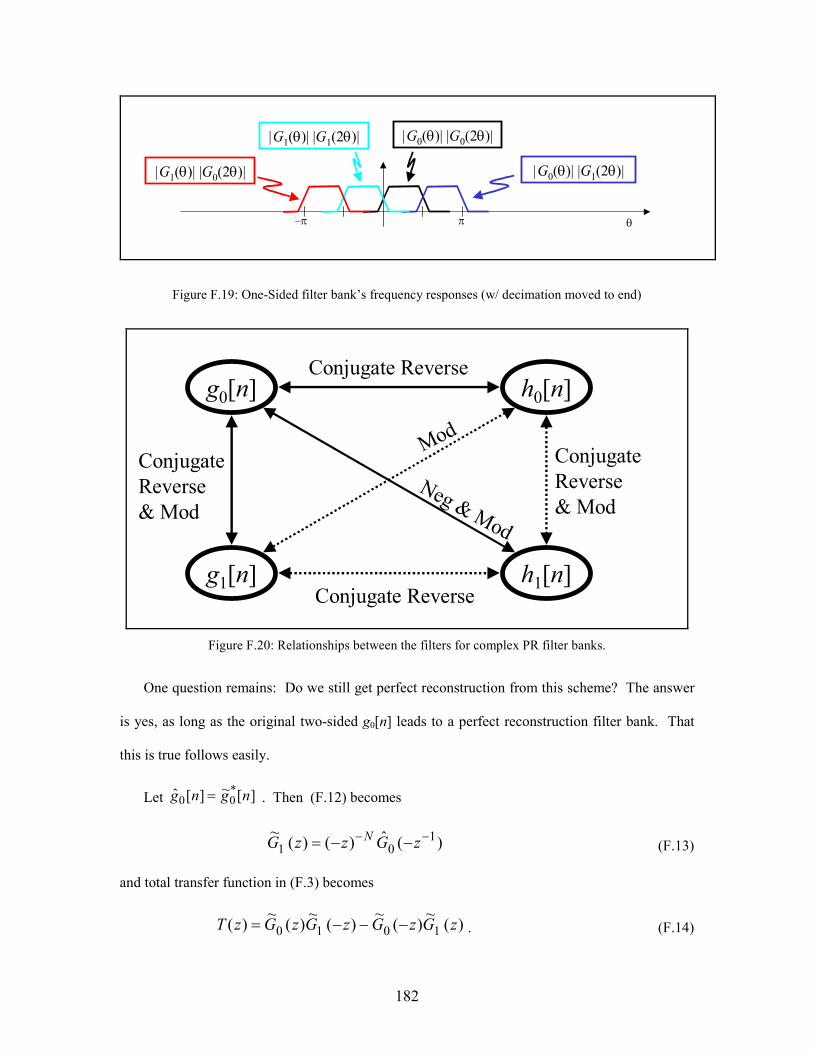
182

π–π θ

|G0(θ)| |G0(2θ)|

|G0(θ)| |G1(2θ)||G1(θ)| |G0(2θ)|

|G1(θ)| |G1(2θ)|

Figure F.19: One-Sided filter bank’s frequency responses (w/ decimation moved to end)

g0[n] h0[n]

g1[n] h1[n]

Conjugate Reverse

Conjugate Reverse

Conjugate

Reverse

& Mod

Conjugate

Reverse

& Mod

Mod

Neg & Mod

Figure F.20: Relationships between the filters for complex PR filter banks.

One question remains: Do we still get perfect reconstruction from this scheme? The answer

is yes, as long as the original two-sided g0[n] leads to a perfect reconstruction filter bank. That

this is true follows easily.

Let ][~][ˆ *00 ngng = . Then (F.12) becomes

)(ˆ)()(~ 1

01−− −−= zGzzG N

(F.13)

and total transfer function in (F.3) becomes

)(~

)(~

)(~

)(~

)( 1010 zGzGzGzGzT −−−= . (F.14)

183

which after substituting (F.13) becomes

[ ])(ˆ)(~

)(ˆ)(~

)( 1

00

1

00

−−− −−−= zGzGzGzGzzT N. (F.15)

where the part in front of the brackets is a pure delay needed for causality. To get PR we need the

frequency response of the part in the brackets to be constant over frequency. To check this we

have

)(~

)(~

)(~

)(~

)(ˆ)(~

)(ˆ)(~

*00

*00

100

100

πθπθθθ −−−

↓

−−− −−

GGGG

zGzGzGzG

, (F.16)

where the conjugated terms in bottom of (F.16) come from

)(~

][~][~

][~)(ˆ

*0

*

0*0

*0

10

θ

θθ

G

engeng

zngzG

n

nj

n

nj

n

n

=

=→

=

∑∑

∑

−+

+−

, (F.17)

Then the bottom of (F.16) becomes

1)(~

)(~ 2

0

2

0 =−+ πθθ GG . (F.18)

That this is true whenever the original filter satisfies (F.8) follows from

1)()(

)2/()2/()(~

)(~

2

0

2

0

2

0

2

0

2

0

2

0

=−+=

−−+−=−+

πξξ

ππθπθπθθ

GG

GGGG

, (F.19)

where we have used a change of variables.

184

BIBLIOGRAPHY

185

BIBLIOGRAPHY

[1] T. M. Cover, J. A. Thomas, Elements of Information Theory, John Wiley& Sons,

1991

[2] K. Fukunaga, Introduction to Statistical Pattern Recognition, Second Edition,

Academic Press, 1990

[3] R. C. Gonzalez and R. E. Woods, Digital Image Processing, Second Edition, NJ:

Prentice Hall, 2001

[4] S. Kay, Fundamentals of Statistical Signal Processing: Estimation Theory,

Englewood Cliffs, NJ: Prentice Hall, 1993.

[5] S. Kay, Fundamentals of Statistical Signal Processing: Detection Theory,

Englewood Cliffs, NJ: Prentice Hall, 1993.

[6] H. Lutkepohl, Handbook of Matrices, John Wiley & Sons, 1996

[7] S. Mallat, A Wavelet Tour of Signal Processing, Second Edition, Academic Press,

1999

[8] A. Mertins, Signal Analysis, Wavelets, Filter Banks, Time-Frequency Transforms

and Applications, John Wiley& Sons, 1999

[9] T. K. Moon and W. C. Stirling, Mathematical Methods and Algorithms for Signal

Processing, Upper Saddle River, NJ: Prentice Hall, 1999

[10] K. Sayood, Introduction to Data Compression, Second Edition, Academic Press,

1996

[11] D. S. Taubman and M. W. Marcellin, JPEG2000, Image Compression

Fundamentals, Standards and Practice, Kluwer Academic Publishers, 2002

[12] R. R. Brooks, P. Ramanathan, and A. M. Sayeed, “Distributed target classificiation

and tracking in sensor networks,” Proceedings of the IEEE, Vol. 91, No. 8, August

2003, pp. 1163-1171

[13] J. C. Chen, K. Yao, and R. E. Hudson, “Source localization and beamforming,”

IEEE Signal Processing Magazine, March 2002, pp. 30-39

[14] D. Li, K. D. Wong, Y. H. Hu and A. M. Sayeed, “Detection, classification, and

tracking of targets,” IEEE Signal Processing Magazine, March 2002, pp. 17-29

[15] G. J. Pottie and W. J. Kaiser, “Wireless integrated network sensors,”

Communications of the ACM, Vol. 43, No. 5, May, 2000, pp.52-58

[16] S. S. Pradhan, J. Kusuma, and K. Ramchandran, “Distributed compression in a

dense microsensor network,” IEEE Signal Processing Magazine, pp. 51– 60,

March 2002.

[17] A. Scaglione and S. Servetto, “On the interdependence of routing and data

compression in multi-hop sensor networks,” MOBICOM’02, Sept. 23 – 26, 2002,

Atlanta, Ga.

[18] S. Tilak, N. B. Abu-Ghazaleh, and W. Heinzelman, “A taxonomy of wireless

micro-sensor network models,” ACM Mobile Computing and Communications

Review (MC2R), vol. 6, pp. 1 – 8, April 2002.

[19] F. Zhao, J. Shin, and J. Reich, “Information-driven dynamic sensor collaboration,”

IEEE Signal Processing Magazine, March 2002, PP. 61-72

186

[20] W. Heinzelman, A. Chandrakasan, and H. Balakrishnan, “Energy-efficient

communication protocol for wireless microsensor networks,” Proc. Of the Hawaii

Conf. on System Science, Jan. 2000

[21] M. Chen and M. L. Fowler, "Data compression trade-offs for multiple estimates

with application to emitter location" submitted to IEEE Signal Processing.

[22] M. Chen and M. L. Fowler, “Geometry-adaptive data compression for

TDOA/FDOA location,” Proceedings of the IEEE International Conference on

Acoustic, Speech and Signal Processing (ICASSP'2005), Philadelphia, PA, Mar.

18-23, 2005.

[23] M. Chen, M.L. Fowler and S. Zhang, “Standards-compatible compression for

automated image recognition in sensor networks,” in Mathematics and

Applications of Data/Image Coding, Compression, and Encryption VI, Mark S.

Schmalz, Editor, Proceedings of SPIE, Vol. 5208, San Diego, CA, August 5 – 7,

2003

[24] M. Chen and M.L. Fowler, “Optimizing non-MSE distortion for data compression

in emitter location systems,” the 37th Conference on Information Sciences and

Systems (CISS’2003), Johns Hopkins University, March 12-14, 2003.

[25] M. Chen and M. L. Fowler, “Non-MSE data compression for emitter location for

radar pulse trains,” in Mathematics and Applications of Data/Image Coding,

Compression, and Encryption VI, Mark S. Schmalz, Editor, Proceedings of SPIE,

Vol. 5208, San Diego, CA, August 5 – 7, 2003

[26] M. Chen and M. L. Fowler, “The importance of data compression for energy

efficiency in sensor networks,” Proceedings of Conference on Information Science

and Systems, Johns Hopkins University, March 12 – 14, 2003.

[27] M. Chen and M. L. Fowler, “Data Compression Trade-Offs for Multiple Inferences

in Sensor Networks,” Proceedings of Conference on Information Science and

Systems, Princeton University, March 17 – 19, 2004.

[28] M. Chen, M.L. Fowler and S. Zhang, “Standards-compatible compression for

automated image recognition in sensor networks,” in Mathematics and

Applications of Data/Image Coding, Compression, and Encryption VI, Mark S.

Schmalz, Editor, Proceedings of SPIE, Vol. 5208, San Diego, CA, August 5 – 7,

2003

[29] A. Ortega and K. Ramchandran, “Rate distortion methods for image and video

compression,” IEEE Signal Processing Magazine, vol. 15, Nov. 1998, pp. 23 – 50.

[30] R. Gray and D. Neuhoff, “Quantization,” IEEE Trans. Information Theory, Vol. 44,

No. 6, pp. 1 – 63, October 1998.

[31] V. K. Goyal, “Theoretical foundations of transform coding,” IEEE Signal

Processing Magazine, September, 2001. pp. 9-21

[32] M. Effros, “Optimal modeling for complex system design,” IEEE Signal

Processing Magazine, November 1998, pp. 51-73

[33] Y. Shoham and A. Gersho, “Efficient bit allocation for an arbitrary set of

quantizers,” IEEE Trans. on Acoustics, Speech, and Signal Processing, 36(9):

1445-1453, 1988.

[34] M. Di. Discegli and M. Longo, “Decentralized encoding of a remote source,”

Signal Processing, 55 (1996), pp. 15 – 29.

187

[35] T. J. Flynn and R. M. Gray, “Encoding of correlated observations,” IEEE

Transactions on Information Theory, vol. IT-33, no. 6, Nov. 1987, pp. 773 – 211.

[36] J. A. Gubner, “Distributed estimation and quantization,” IEEE Transactions on

Information Theory, vol. 39, no. 4, July 1993, pp. 1456 – 1459.

[37] T. S. Han and S. Amari, “Parameter estimation with multiterminal data

compression,” IEEE Transactions on Information Theory, vol. 41, no. 6, Nov. 1995,

pp. 1802 – 1833.

[38] H.V. Poor, “Fine quantization in signal detection and estimation,” IEEE

Transactions on Information Theory, vol. 34, no. 5, Sept. 1988, pp. 960-972

[39] W. Lam and A. R. Reibman, “Design of quantizers for decentralized estimation

systems,” IEEE Transactions on Communications, vol. 41, no. 11, Nov. 1993, pp.

1602 – 1605.

[40] Z. Zhang and T. Berger, “Estimation via compressed information,” IEEE

Transactions on Information Theory, vol. 34, no.2, March 1988, pp. 198-211.

[41] L. Vasudevan, A. Ortega, U. Mitra, “Application specific compression for time

delay estimation in sensor networks,” Proceedings of the First ACM international

Conference on Embedded Networked Sensor Systems, Nov. 2003, Los Angeles,

CA, pp. 243-253

[42] S. A. Kassam, “Optimum quantization for signal detection,” IEEE Transactions on

Communications, Vol. COM-25, No. 5, May 1977, pp. 479-484

[43] H. V. Poor, “A companding approximation for the statisitical divergence of

quantized data,” in Proc. of IEEE Conf. Decision and Control, San Antonio, TX,

Dec, 1983

[44] B. Picinbono and P. Duvaut, “Optimum quantization for detection,” IEEE Trans.

on Communications, vol. 36, no. 11, pp. 1254-1258, Nov. 1988

[45] J. N. Tsitsiklis, “Extremal properties of likelihood ratio quantizers,” IEEE Trans.

on Communications, vol. 41, no. 4, pp. 550-558, Apr. 1993

[46] K. L. Oehler and R. Gray, “Combining image compression and classification using

vector quantization,” IEEE Transaction on Information Theory, Vol.17, No. 5, May,

1995, pp. 461-473

[47] K. O. Perlmutter, S. M. Perlmutter, et al., “Bayes risk weighted vector quantization

with posterior estimation for image compression and classification,” IEEE Trans.

on Image Processing, vol. 5, no.2, pp. 347-360, Feb. 1996

[48] H. V. Poor and J. B. Thomas, “Applications of Ali-Silvey distance measures in the

design of generalized quantizers,” IEEE Trans. on Communications, vol. COM-25,

pp.893-900, Sep. 1977

[49] G. R. Benitz and J. A. Bucklew, “Asymptotically optimal quantizers for detection

of I.I.D. Data,” IEEE Trans. on Inform. Theory, vol. 35, no. 2, pp, 316-325, Mar.

1989

[50] M. Longo, T. D. Lookabaugh, and R. Gray, “Quantization for decentralized

hypothesis testing under communication constraints,” IEEE Transaction on

Information Theory, Vol. 36, No. 2, Mar. 1990, pp. 241-255.

[51] A. Jain, P. Moulin, M. Miller, K Ramchandran, “Information-theoretic bounds on

target recognition performance based on degraded image data,” IEEE Transactions

on Pattern Analysis and Machine Intelligence, Vol.24, No.9, Sep. 2002, pp.1153-

1166

188

[52] A.D. Lanerman, J.A. O’Sullivan, M. I. Miller, “Kullback-Leibler distances for

quantifying clutter and models,” Opt. Eng. 38(12) 2134-2146, December 1999

[53] B. Aazhang and H. V. Poor, “On optimum and nearly optimum data quantization

for signal detection,” IEEE Transactions on Communications, Vol. COM-32, No. 7,

July 1984.

[54] L. Yaroslavsky, “Advanced image processing lab: a tutorial,” presented at

EUSIPCO2000, Tampere, Finland, Sept. 2000.

[55] B. Walls and A. Mahalanobis, “Performance of the MACH filter and DCCF

algorithms in presence of data compression,” Proc. SPIE 3718, 376-387, 1999

[56] S. R. F. Sims, “Data compression issues in automatic recognition and the

measuring of distortion,” Opt. Eng. 36, 2671-2674 (1997)

[57] J. Wozencraft and I. Jacobs, Principles of Communication Engineering, New York:

Wiley, 1965

[58] A. Krasnopeev, J-J. Xiao and Z-Q. Luo, “Minimum Energy Decentralized

Estimation In Sensor Networks with Correlated Sensor Noise,” Proceedings of the

IEEE International Conference on Acoustic, Speech and Signal Processing

(ICASSP'2005), Philadelphia, PA, Mar. 18-23, 2005.

[59] R. M. Gray and T. G. Stockham, Jr., “Dithered Quantizers,” IEEE Trans. on Inform.

Theory, vol. 39, pp. 805 - 812, May 1993.

[60] M. L. Fowler and M. Chen, “Integer Optimization Methods for Non-MSE Data

Compression for Emitter Location,” in Mathematics and Applications of

Data/Image Coding, Compression, and Encryption V, Mark S. Schmalz, Editor,

Proceedings of SPIE, Vol. 4793, Seattle, WA, July 8 – 11, 2002.

[61] R. M. Gray and T. G. Stockham, Jr., “Dithered Quantizers,” IEEE Trans. on Inform.

Theory, vol. 39, pp. 805 - 812, May 1993.

[62] R. M. Gray, “Quantization Noise Spectra”, IEEE Transactions on Information

Theory, Vol. 36, No. 6, Nov. 1990.

[63] V. K. Goyal, “Theoretical Foundations of Transform Coding,” IEEE Signal

Processing Magazine, September 2001, pp.9-21

[64] H. V. Poor and J. B. Thomas, “Application of Ali-Silvey distance measures in the

design of generalized quantizers for binary decision systems,” IEEE Transactions

on Communications, Vol. COM-25, No.9, Sept. 1977.

[65] L. Vasudevan, A. Ortega, U. Mitra, “Application specific compression for time

delay estimation in sensor networks,” Proceedings of the First ACM International

Conference on Embedded Networked Sensor Systems, Nov. 2003, Los Angeles, CA,

pp. 243-253. .

[66] D. Torrieri, “Statistical Theory of Passive Location Systems,” IEEE Trans. on

Aerospace and Electronic Systems, pp. 183 - 198, March 1984.

[67] S. Stein, “Differential Delay/Doppler ML Estimation with Unknown Signals,”

IEEE Trans. on Signal Processing, pp. 2717 - 2719, August 1993.

[68] T. Berger and R. Blabut, “Coherent estimation of differential delay and differential

doppler,” Proceedings of the 1984 Conference on Information Sciences and

Systems, Princeton University, pp.537-541, 1984

[69] S. Stein, “Algorithms for ambiguity function processing,” IEEE Transaction on

Acoustics, Speech, and Signal Processing, Vol. ASSP-29, No.3, Jun. 1981, pp.588-

599

189

[70] J. Krim and M. Viberg, “Two decades of array signal processing research: The

parametric approach,” IEEE Signal Processing Mag. vol. 13, pp. 67-94, July 1996.

[71] P. Stoica. and R. Moses, Introduction to spectral analysis, Upper Saddle River, NJ:

Prentice Hall, 1997

[72] I. Daubechies, Ten lectures on wavelets, Society for industrial and Applied

Mathematics, 1992

[73] H.V. Poor, An Introduction to Signal Detection and Estimation. New York:

Springer-Verlayge.

[74] J. Watkinson, The MPEG handbook : MPEG-1, MPEG-2, MPEG-4 , Focal Press,

2004

[75] M. L. Fowler and M. Chen, “Fisher-Information-Based Data Compression for

Estimation Using Two Sensors,” to appear in IEEE Transactions on Aerospace and

Electronic Systems.

[76] D. C. Kammer, “Sensor placement for on-orbit modal identification and correlation

of large space structures,” J. Guidance Control & Dynamics, Vol. 14, No. 2, pp.

251 – 259, March-April 1991.

[77] W. L. Poston and R. H. Tolson, “Maximizing the determinant of the information

matrix with the effective independence distribution method,” J. Guidance Control

& Dynamics, Vol. 15, No. 6, pp. 1513 – 1514, Nov. – Dec. 1992.

[78] V. V. Fedorov, Theory of Optimal Experiments, translated and edited by W. J.

Studden and E. M. Klimko, Academic Press, New York, 1972.

[79] M. Chu, H. Haussecher, and F. Zhao, “Scalable Information-Driven and Routing

for Ad Hoc Heterogeneous Sensor Networks,” International Journal of High

Performance Computing Applications, 2002

[80] H. Wang, G. Pottie, H. Yao and D. Estrin, “Entropy-based Sensor Selection

Heuristic for Target Localization,” IPSN’04, April 26-27, 2004, Berkeley,

California, USA.

[81] H. L. Resnikoff and C. S. Burrus, “Relationship between the Fourier transform and

the wavelet transform,” SPIE, vol. 1348, Advanced Signal-Processing Algorithms,

Architectures, and Implementations, 1990, pp. 291-300

[82] N. Hess-Nielsen and M. V. Wickerhauser, “Wavelet and time-frequency analysis,”

Proceeding of the IEEE, vol. 84, no. 4, April, 1996, pp. 523-540

[83] D. B. Percival and A. T Walden, Wavelet Methods for Time Series Analysis,

Cambridge University Press, 2000

[84] M. Fowler, “Analysis of Single-Platform Passive Emitter Location With Terrain

Data,” IEEE Transactions on Aerospace and Electronic Systems, vol. 37, no. 2,

April. 2001, pp. 495-507

[85] S. Cui, A. J. Goldsmith, and A. Bahai, “Energy-constrained Modulation

Optimization,” to appear at IEEE Trans. on Wireless Communications, September,

2005.

[86] G. B. Giannakis, Y. Hua, P. Stoica and L. Tong, Signal Processing Advances in

Wireless and Mobile Communications, trends in Signal-User and Multi-User

Systems - vol.2, 2001 Prentice Hall PTR.

[87] M. L. Fowler, “Non-MSE Wavelet-Based Data Compression for Emitter Location,”

in Mathematics and Applications of Data/Image Coding, Compression, and

190

Encryption IV, Mark S. Schmalz, Editor, Proceedings of SPIE, Vol. 4475, San

Diego, CA, July 29 – August 3, 2001, pp. 13 – 22

data compression for inference tasks in wireless sensor networks

Documents