data-driven many-body models for molecular fluids: co2/h2o
TRANSCRIPT

doi.org/10.26434/chemrxiv.11288465.v1
Data-Driven Many-Body Models for Molecular Fluids: CO2/H2O Mixturesas a Case StudyMarc Riera, Eric Yeh, Francesco Paesani
Submitted date: 27/11/2019 • Posted date: 06/12/2019Licence: CC BY-NC-ND 4.0Citation information: Riera, Marc; Yeh, Eric; Paesani, Francesco (2019): Data-Driven Many-Body Models forMolecular Fluids: CO2/H2O Mixtures as a Case Study. ChemRxiv. Preprint.https://doi.org/10.26434/chemrxiv.11288465.v1
In this study, we extend the scope of the many-body TTM-nrg and MB-nrg potential energy functions (PEFs),originally introduced for halide ion–water and alkali-metal ion–water interactions, to the modeling of carbondioxide (CO2) and water (H2O) mixtures as prototypical examples of molecular fluids. Both TTM-nrg andMB-nrg PEFs are derived entirely from electronic structure data obtained at the coupled cluster level of theoryand are, by construction, compatible with MB-pol, a many-body PEF that has been shown to accuratelyreproduce the properties of water. Although both TTM-nrg and MB-nrg PEFs adopt the same functional formsfor describing permanent electrostatics, polarization, and dispersion, they differ in the representation ofshort-range contributions, with the TTM-nrg PEFs relying on conventional Born-Mayer expressions and theMB-nrg PEFs employing multidimensional permutationally invariant polynomials. By providing a physicallycorrect description of many-body effects at both short and long ranges, the MB-nrg PEFs are shown toquantitatively represent the global potential energy surfaces of the CO2–CO2 and CO2–H2O dimers and theenergetics of small clusters as well as to correctly reproduce various properties in both gas and liquid phases.Building upon previous studies of aqueous systems, our analysis provides further evidence for the accuracyand efficiency of the MB-nrg framework in representing molecular interactions in fluid mixtures at differenttemperature and pressure conditions.
File list (3)
download fileview on ChemRxivmany-body_mixtures.pdf (3.97 MiB)
download fileview on ChemRxivsupp_info.pdf (151.39 KiB)
download fileview on ChemRxivco2_h2o.pdf (266.17 KiB)

Data-Driven Many-Body Models for Molecular
Fluids: CO2/H2O Mixtures as a Case Study
Marc Riera,∗,† Eric P. Yeh,† and Francesco Paesani∗,†,‡,¶
†Department of Chemistry and Biochemistry, University of California San Diego,
La Jolla, California 92093, United States
‡Materials Science and Engineering, University of California San Diego,
La Jolla, California 92093, United States
¶San Diego Supercomputer Center, University of California San Diego,
La Jolla, California 92093, United States
E-mail: [email protected]; [email protected]
Abstract
In this study, we extend the scope of the many-body TTM-nrg and MB-nrg potential
energy functions (PEFs), originally introduced for halide ion–water and alkali-metal
ion–water interactions, to the modeling of carbon dioxide (CO2) and water (H2O)
mixtures as prototypical examples of molecular fluids. Both TTM-nrg and MB-nrg
PEFs are derived entirely from electronic structure data obtained at the coupled clus-
ter level of theory and are, by construction, compatible with MB-pol, a many-body
PEF that has been shown to accurately reproduce the properties of water. Although
both TTM-nrg and MB-nrg PEFs adopt the same functional forms for describing per-
manent electrostatics, polarization, and dispersion, they differ in the representation
of short-range contributions, with the TTM-nrg PEFs relying on conventional Born-
Mayer expressions and the MB-nrg PEFs employing multidimensional permutationally
1

invariant polynomials. By providing a physically correct description of many-body ef-
fects at both short and long ranges, the MB-nrg PEFs are shown to quantitatively
represent the global potential energy surfaces of the CO2–CO2 and CO2–H2O dimers
and the energetics of small clusters as well as to correctly reproduce various properties
in both gas and liquid phases. Building upon previous studies of aqueous systems, our
analysis provides further evidence for the accuracy and efficiency of the MB-nrg frame-
work in representing molecular interactions in fluid mixtures at different temperature
and pressure conditions.
1 Introduction
Carbon dioxide (CO2) plays a central role in the carbon cycle, representing the primary
carbon source for life on Earth.1 CO2 is the fourth most abundant gas in the atmosphere,
where it acts as a greenhouse gas,2 and dissolves in water to form carbonic acid (H2CO3)
whose equilibrium with bicarbonate (HCO−3 ) and carbonate (CO2−3 ) has significant impact
on the pH of the oceans,3,4 which, in turn, act as an enormous carbon sink,5 containing about
fifty times more carbon than the atmosphere. Under pressure, CO2 dissolved in water form
clathrate hydrates, cage-like structures of hydrogen-bonded water molecules hosting CO2
as guest species.6 In living systems, CO2 is the end product of cellular respiration,7 while
photosynthetic organisms combine CO2 and H2O to produce carbohydrates.8 Combustion
processes taking place in both natural (e.g., wildfires) and anthropogenic (e.g., combustion
engines) settings are major sources of CO2.9 In the chemical industry, CO2 is primarily used
in the production of urea, with smaller fractions used to produce methanol, and metal car-
bonates and bicarbonates.10 In the context of renewable energy applications, electrochemical
CO2 reduction represents a potential route to producing fuels.11 In the food industry, CO2
is used in carbonated soft drinks as well as a propellant and acidity regulator.12 In the liquid
phase, CO2 is a good solvent for lipophilic organic compounds and is used in the pharmaceu-
tical and chemical industries as a less toxic alternative to more traditional solvents such as
2

organochlorines.13 Supercritical CO2 is used in dry cleaning because of its low toxicity and
efficient solvent properties.14 Finally, CO2 is used in extinguishers and refrigerant systems
as well as in oil recovery processes.15
Given their relevance for geochemical applications, neat CO2 and CO2/H2O mixtures
have been extensively studied at the macroscopic level. This has led to the development of
several equation-of-state (EOS) models that are widely used to describe the thermodynamic
properties of these mixtures, sometimes in combination with methane and various salts.16–23
At the molecular level, vibrational spectroscopy is used to characterize structure and dy-
namics of CO2 clusters and clathrates, liquid and supercritical CO2 as well as the properties
of CO2 in mixtures with water, small alcohols and hydrocarbons, and in ionic liquids.24–34
Recently, X-ray diffraction has been used to determine the local structure of liquid CO2 at
pressures up to 10 GPa and temperatures from 300 to 709 K.35
From a theoretical standpoint, electronic structure calculations and molecular dynamics
(MD) simulations have been used to model the energetics as well as the structural, thermody-
namic, and dynamical properties of CO2, in both single- and multi-component systems.36–57
Most of the early molecular models adopted relatively simple functional forms parameterized
to reproduce vapor/liquid equilibrium properties.36–38,40 More recently, several models that
include many-body effects, either implicitly or explicitly, have been proposed.51,52,55,57,58 An
analytical representation of the potential energy surface of the CO2 dimer (with rigid CO
bonds) was derived from reference energies obtained at the symmetry adapted perturbation
theory (SAPT) level and used to calculate the second virial coefficient that was found to be
in good agreement with the corresponding experimental data.39 SAPT calculations were also
used to develop an implicit many-body model of CO2 with rigid CO bonds and polarization
effects represented by the Drude model.51 After empirically reducing the SAPT-calculated
dispersion energy by ∼6%, good agreement with experiment was obtained for several prop-
erties of CO2 in the gas, liquid, and supercritical phases. Subsequent refinement of this
polarizable model through inclusion of an explicit three-body (3B) term led to an accurate
3

description of both gas and condensed-phase properties without relying on any empirical pa-
rameterization, suggesting that two-body (2B) models effectively exploit error cancellation
to achieve satisfactory results.52 A Drude model was also used to develop a different polariz-
able model (still with rigid CO bonds) that was shown to reproduce several thermodynamic
and transport properties of the liquid phase.55 However, similar results were also obtained
with a nonpolarizable model, which led to the conclusion that the properties of liquid CO2
are not significantly affected by many-body polarization. Subsequent simulations carried
out for CO2/H2O mixtures demonstrated current difficulties in determining CO2 solubility
in water as well as the water composition in CO2-rich phases using polarizable models.56
Building upon recent progress in the development of explicit many-body potential energy
functions (PEFs) capable of describing molecular interactions with chemical accuracy,59–73
several PEFs for CO2 have been proposed. A 2B PEFs for CO2–H2O was derived from
electronic structure calculations carried out at the coupled cluster level of theory.57 This
2B PEF was used to calculate the intramolecular vibrational frequencies of the CO2–H2O
dimer, which were found to be in good agreement with the available experimental data
as well as to investigate the structure and vibrational modes of the CO2(H2O)20 cluster
corresponding to the 512 water cage of the CO2 hydrate clathrates. In the simulations of
CO2(H2O)20, the interactions between the water molecules were described by the many-
body MB-pol PEF62–64 that accurately reproduces the properties of water from the gas to
the condensed phase.74,75 More recently, a 2B PEF for CO2 was developed from CCSD(T)-
F12b/aug-cc-pVTZ reference data and used in the analysis of both structures and energetics
of small (CO2)N clusters with N ≤ 13 which were found to be in good agreement with
results obtained using density functional theory (DFT) with the M06-2X and B2PLYP-D
functionals.58
In this study, we present full-dimensional many-body PEFs for neat CO2 and CO2/H2O
mixtures developed within the TTM-nrg and MB-nrg theoretical/computational frameworks
originally introduced to represent the interactions of halide68,69 and alkali-metal ions70,71
4

with water. Through a detailed analysis of the energetics of small clusters, many-body
contributions, virial coefficients of gas mixtures, and structural properties of liquid mixtures,
we demonstrate that the MB-nrg PEFs provide highly accurate representations of neat CO2
and CO2/H2O mixtures from the gas to the condensed phase. The article is organized
as follows: Section 2 describes the functional forms of both TTM-nrg and MB-nrg PEFs,
training sets, and fitting procedure. Section 3 presents comparisons of the TTM-nrg and MB-
nrg PEFs with the ωB97M-V functional76 and Møller-Plesset perturbation theory (MP2) as
well as various experimental data. Finally, Section 4 summarizes the main points of our
study and provides an outlook of future research on many-body PEFs.
2 Theoretical and Computational Methodology
2.1 TTM-nrg and MB-nrg functional forms
The total energy of a system containing N (atomic and/or molecular) monomers can be
formally expressed as
EN(1, . . . , N) =N∑i=1
V 1B(i) +N∑i<j
V 2B(i, j) +N∑
i<j<k
V 3B(i, j, k) + · · ·+ V NB(1, . . . , N), (1)
which is known as the many-body expansion (MBE) of the energy.77 In Eq. 1, V 1B(i) = 0 and
V 1B(i) = E(i)−Eeq(i) for atomic and molecular monomers, respectively. In the latter case,
V 1B(i) corresponds to the one-body (1B) energy required to deform an individual monomer
from its equilibrium geometry, and V nB are the n-body (nB) energies defined recursively as
V nB(1, . . . , n) = En(1, . . . , n)−∑i
V 1B(i)−∑i<j
V 2B(i, j)− . . .
−∑
i<j<···<n−1
V (n-1)B(i, j, . . . , (n− 1))
(2)
5

Since the MBE converges quickly for non-metallic systems (such as CO2 and H2O),78 Eq. 1
provides a rigorous and efficient framework for the development of full-dimensional PEFs
in which each individual term of the MBE can be separately determined from high-level
electronic structure calculations.
Starting from Eq. 1 and building upon the accuracy and computational efficiency demon-
strated by MB-pol in predicting the properties of water across different phases,74,75 two fam-
ilies of MB PEFs (TTM-nrg for “Thole-type model energy” and MB-nrg for “many-body
energy”) have recently been introduced to describe halide–water68,69 and alkali-metal ion–
water70,71 interactions, which have then be applied to model ion–water systems in the gas and
the liquid phase.79–86 Both TTM-nrg and MB-nrg PEFs rely on MB-pol for the description
of all water properties (i.e., water monomer distortion, dipole moment, and polarizability,
as well as water–water interactions) and differ in the functional forms employed to represent
the solute–water interactions. In this study, the TTM-nrg and MB-nrg families are further
extended to allow for the development of MB PEFs describing molecular interactions in
generic molecular fluids, with a specific focus on neat CO2 and CO2/H2O mixtures.
The TTM-nrg 1B term representing an isolated CO2 molecule adopts a functional form
similar to those employed by common force fields, which is expressed in Eq. 3 as a sum
of the two bond stretching energies (V bond) and the angle bending energy (V angle). Each
bond energy is described by a Morse potential, while the bending energy is represented by a
harmonic potential,
V 1B = V bond + V angle
V bond = De
(1− e−a(rCO1
−reqCO))2
+De
(1− e−a(rCO2
−reqCO))2
V angle = 12k(φ− φeq)2
(3)
All TTM-nrg parameters in Eq. 3 are derived from fits to high-quality ab initio data (see
Section 2.4).
In contrast, the 1B term of the corresponding MB-nrg PEF is represented by a permu-
6

tationally invariant polynomial (PIP),87
V 1B = V 1Bpoly({ξ}) (4)
where {ξ} corresponds to a set of monomials that are functions of the distances between the
C and O atoms of the CO2 molecule (see Supporting Information). In V 1Bpoly, permutational
invariance is enforced between the two equivalent O atoms of the CO2 molecule, and con-
tains 21 symmetrized terms: 2 1st-degree monomials, 4 2nd-degree monomials, 6 3rd-degree
monomials, and 9 4th-degree monomials. Consequently, V 1Bpoly contains 21 linear parameters
and 4 nonlinear parameters that are optimized to reproduce the reference ab initio data (see
Section 2.4). In both TTM-nrg and MB-nrg, the zero in the 1B energy is set to the energy
of an isolated CO2 molecule in its equilibrium geometry.
Both TTM-nrg and MB-nrg PEFs describe many-body contributions to the interaction
energies in neat CO2 and CO2/H2O mixtures through the following expression:
V MBTTM-nrg = V 2B, perm
TTM + V NB, indTTM + V 2B
short + V 2Bdisp (5)
where V 2B, permTTM represents 2B permanent electrostatic contributions and V NB, ind
TTM represents
NB polarization contributions that are described by the extended Thole-type model originally
introduced with the TTM4-F water PEF.88
In the TTM-nrg PEFs, the short-range 2B term V 2Bshort, describing repulsive interactions
between pairs of molecules, is represented by a sum of pairwise Born-Mayer functions between
all atoms of the two monomers,89
V 2Bshort =
∑k
V krep (6)
V krep =
∑i∈M1j∈M2
Aije−bijRij (7)
7

where Rij are interatomic distances between atoms i and j of monomers M1 (i.e., CO2) and
M2 (i.e., CO2 or H2O), and Aij and bij are fitting parameters. Similarly, the 2B dispersion
energy, V 2Bdisp, is represented by a sum of pairwise additive contributions,
V 2Bdisp =
∑k
V kdisp (8)
V kdisp = f(Dij, Rij)
C6,ij
R6ij
(9)
where
f(D,R) = 1− exp(−DR)6∑
n=0
DR
n!(10)
is the Tang-Toennies damping function,90 and C6,ij are interatomic dispersion coefficients
derived from ab initio data (see Section 2.4).
The corresponding MB-nrg PEFs employ the same functional forms for V 2B, permTTM , V NB, ind
TTM ,
and V 2Bdisp as the TTM-nrg PEFs, but express V 2B
short in terms of PIPs, V 2Bpoly,87 that smoothly
switch to zero when the distance between the two monomers (RAB) becomes larger than a
predefined cutoff value,
V 2Bshort = s2
(RAB −Rin
Rout −Rin
)V 2B
poly (11)
where s2(x) is a switching function defined as
s2(x) =
1 if x < 0
(1 + cos(x)) ∗ 0.5 if 0 ≤ x < 1
0 if 1 ≤ x
(12)
The inner (Rin) and outer (Rout) cutoff radii in Eq. 11 are chosen to guarantee a continuous
transition between short- and long-range components of the total V 2B interaction energy.
Specifically, Rin corresponds to the C–C (for CO2-CO2) and C–O (for CO2-H2O) distances at
which the total and electrostatic (i.e., V 2B, permTTM +V NB, ind
TTM ) energies differ by 0.01 kcal/mol or
less, and Rout = Rin + 1.0 A. Following these criteria, Rin and Rout were set to 8.0 A and
8

9.0 A for CO2–CO2 and CO2–H2O, respectively.
V 2Bpoly is a function of the distances (dn) between all physical atoms (C and O for CO2,
and O and H for H2O) as well as the two lone pairs (L1 and L2) of the MB-pol water
molecule as defined in Ref. 62. All distances dn entering the expression of V2Bpoly, along with
the corresponding variables for the CO2–CO2 and CO2–H2O 2B terms are reported in the
Supporting Information. Specifically, V 2Bpoly is a polynomial function of a set of monomials
{ξ}, with permutational invariance enforced with respect to equivalent atoms within the
dimer. V 2Bpoly for the CO2–CO2 dimer contains a total of 2269 terms: 3 1st-degree monomials,
21 2nd-degree monomials, 110 3rd-degree monomials, 463 4th-degree monomials, and 1672 5th-
degree monomials, resulting in 2269 linear parameters and 15 nonlinear parameters. V 2Bpoly for
the CO2–H2O dimer contains a total of 1653 symmetrized terms: 6 1st-degree monomials, 64
2nd-degree monomials, 311 3rd-degree monomials, and 1272 4th-degree monomials, resulting
in 1653 linear parameters and 21 nonlinear parameters.
2.2 Selection of training and test sets
The 1B training set for the CO2 monomer consists of 1612 configurations extracted from two
different sources. An initial set of configurations was obtained from normal-mode sampling
using a quantum distribution91 performed at three temperatures (0 K, 987 K, and 2008 K).
The lowest temperature was used to obtain configurations around the minimum-energy struc-
ture, while the other two temperatures allow for sampling more distorted configurations since,
when converted to wavenumbers, they correspond to the ab initio frequencies of the bending
and symmetric stretching vibrations of an isolated CO2 molecule. Additional configura-
tions, with energies within 10 kcal/mol of the minimum energy structure, were added from
a uniform multidimensional grid constructed along the CO2 normal modes. To assess the
accuracy of both TTM-nrg and MB-nrg PEFs, an independent test set of 511 configurations
was generated from normal-mode sampling91 performed at 3512 K, corresponding to 2441
cm−1, i.e., the ab initio frequency of the CO2 asymmetric stretching vibration. The test set
9

was specifically constructed to include distorted configurations sampled from a wider energy
distribution than that used to generate the training set.
To ensure a proper representation of the 12-dimensional 2B configurational space as-
sociated with the CO2–CO2 and CO2–H2O dimers, the corresponding training sets were
generated by extracting configurations form different sources, including normal-mode and
random sampling, uniform grids, and MD simulations. A total of 28631 and 28057 configu-
rations were used to train the 2B PIPs of the CO2–CO2 and CO2–H2O PEFs, respectively.
Corresponding test sets, containing 1569 CO2–CO2 and 1768 CO2–H2O dimer configurations
were also generated from the same sources used for the training sets.
2.3 Fitting procedure
Following the same procedure adopted in the development of MB-pol62–64 and MB-nrg PEFs
for halide-water69 and alkali metal ion-water systems,71 the linear and nonlinear parame-
ters of the PIPs used in both CO2–CO2 and CO2–H2O MB-nrg PEFs were optimized using
linear regression and the simplex algorithm, respectively. For the linear parameters, we em-
ployed the Tikhonov regularization (also known as Ridge regression),92 with a regularization
parameter α = 0.0005, to minimize the total χ2
χ2 =∑n∈S
wn[Vpoly(n)− Vref(n)]2 + α2
N∑i=1
c2i (13)
Here, Vref are the reference energies, N is the number of linear terms in the PIPs, n is the
number of configurations in the training set S, and the weights wn are defined as
w(Ei) =
{∆E
Ei − Emin + ∆E
}2
. (14)
In Eq. 14, En is the binding energy of the corresponding dimer n, and ∆E is a parameter
that was set to 15 kcal/mol for both CO2–CO2 and CO2–H2O dimers to guarantee that
10

configurations with En > 15 kcal/mol have weights w(En) ≤ 0.25.
2.4 Electronic structure calculations
Atomic charges for both C and O atoms of CO2 were derived from ChelpG93 calculations
carried out with Q-Chem 5.094 for an isolated CO2 molecule at the DFT level with the meta
GGA, hybrid, and range-separated ωB97M-V functional76 in combination with the aug-cc-
pVTZ basis set.95–99 Dipole polarizabilities of the isolated C and O atoms were computed
at the coupled cluster theory with single, double and perturbative triple excitations, i.e.,
CCSD(T), level of theory using the aug-cc-pV5Z95–99 basis set according to the methodology
described in Ref. 98. The corresponding effective atomic polarizabilities for the CO2 molecule
were determined as
αeff = αfree Veff
Vfree(15)
where Vfree and Veff are the volumes of the isolated C and O atoms, and the effective volumes
of the two atoms in CO2, respectively. Both Vfree and Veff were calculated using the exchange-
dipole moment (XDM) model100–102 as implemented in Q-Chem 5.0.94 The XDM model was
also used to determine the interatomic C6,ij dispersion coefficients in Eq. 9. All XDM
calculations were carried out at the ωB97M-V/aug-cc-pVTZ level of theory. The values of
the C and O charges and polarizabilities, along with the corresponding free and effective
volumes, as well as the Born-Mayer Aij (Eq. 7) and dispersion C6,ij (Eq. 9) coefficients are
reported in the Supporting Information.
All reference energies for the CO2 1B term, and the CO2–CO2 and CO2–H2O 2B terms
were calculated using explicitly correlated coupled cluster theory, i.e., CCSD(T)-F12b,103,104
via a two-point extrapolation105,106 between energy values obtained with the aug-cc-pVTZ
and aug-cc-pVQZ basis sets95–99 for the CO2 monomer, and between energy values obtained
with the aug-cc-pVDZ and aug-cc-pVTZ basis sets95–99 for both CO2–CO2 and CO2–H2O
dimers. Since the aug-cc-pVDZ basis set is relatively small, all dimer energies were corrected
11
for the basis set superposition error (BSSE) using the counterpoise method.107
Optimized structures for (CO2)m and (CO2)m(H2O)n clusters, with m = 1–4, n = 1–4,
and n+m ≤ 4, were obtained using density-fitting second-order Møller-Pleset perturbation
(DF-MP2) theory in combination with the aug-cc-pVQZ basis set.95–99 A gradient conver-
gence threshold of 10−6 a.u was used in these optimizations. All CCSD(T)-F12b and DF-MP2
calculations were carried out with MOLPRO, version 2015.1.108
Reference data for individual many-body contributions to the total interaction energies
of the optimized (CO2)m and (CO2)m(H2O)n clusters were calculated at the CCSD(T)-F12b
level of theory using the SAMBA approach.106 Specifically, 1B and 2B contributions were
obtained from a two-point extrapolation between energies computed using the aug-cc-pVTZ
and aug-cc-pVQZ basis sets, while 3B and 4B contributions were obtained from a two-point
extrapolation between energies computed using the aug-cc-pVDZ and aug-cc-pVTZ basis
sets. Local BSSE corrections, corresponding to computing the kth contribution to the jth-
body term by applying counterpoise corrections only to atoms belonging to the kth cluster,
were applied to the calculations of all 1B to 4B terms.
3 Results
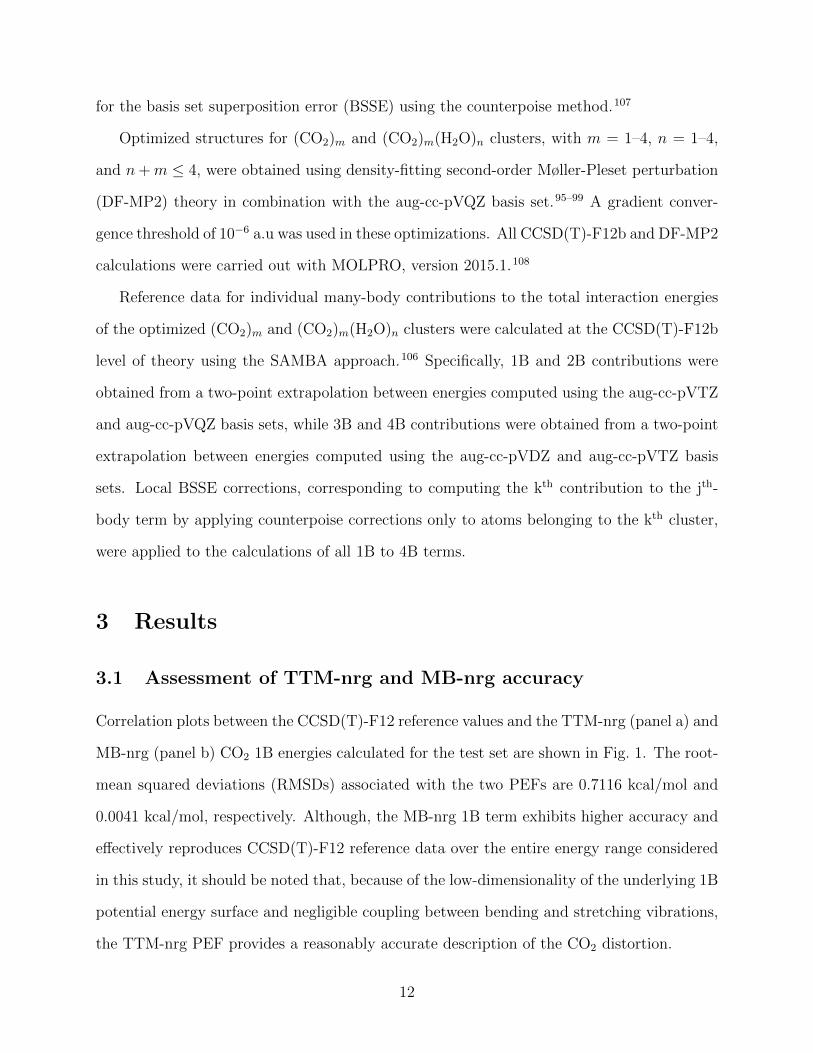
3.1 Assessment of TTM-nrg and MB-nrg accuracy
Correlation plots between the CCSD(T)-F12 reference values and the TTM-nrg (panel a) and
MB-nrg (panel b) CO2 1B energies calculated for the test set are shown in Fig. 1. The root-
mean squared deviations (RMSDs) associated with the two PEFs are 0.7116 kcal/mol and
0.0041 kcal/mol, respectively. Although, the MB-nrg 1B term exhibits higher accuracy and
effectively reproduces CCSD(T)-F12 reference data over the entire energy range considered
in this study, it should be noted that, because of the low-dimensionality of the underlying 1B
potential energy surface and negligible coupling between bending and stretching vibrations,
the TTM-nrg PEF provides a reasonably accurate description of the CO2 distortion.
12

Figure 1: Panels a-b: Correlation plots between the CCSD(T)-F12b reference data and theTTM-nrg (panel a) and MB-nrg (panel b) 1B energies calculated for the CO2 test set.
The differences between the TTM-nrg and MB-nrg PEFs become more pronounced at the
2B level for both the CO2–CO2 and CO2–H2O dimers as demonstrated by the corresponding
correlation plots shown in Fig. 2. For this analysis, the test sets are divided in configu-
rations with low (below 40 kcal/mol, orange and light green for CO2–CO2 and CO2–H2O,
respectively) and high (above 40 kcal/mol, red and dark green for CO2–CO2 and CO2–H2O,
respectively) binding energies (BEs), which are defined as the differences between the dimer
energies and the energies of the individual monomers in their optimized geometries. Con-
sidering only configurations with low BEs, the RMSDs associated with the TTM-nrg and
MB-nrg PEFs for the CO2–CO2 dimer are 0.524 kcal/mol and 0.060 kcal/mol, respectively.
The correlation plots shown in Fig. 2a-b demonstrate that, while the MB-nrg PEF accurately
predicts the interaction strength over the entire energy range, the TTM-nrg PEF tends to
underestimate (overestimate) the interaction strength for configurations with low (high) in-
teraction energies. This implies that the TTM-nrg PEF is unable to correctly reproduce the
anisotropy of the multidimensional potential energy surface, predicting relatively more re-
pulsive interactions for CO2–CO2 configurations in the neighborhood of the minimum-energy
13
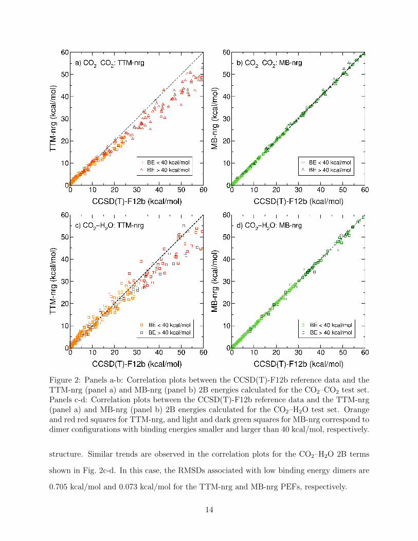
Figure 2: Panels a-b: Correlation plots between the CCSD(T)-F12b reference data and theTTM-nrg (panel a) and MB-nrg (panel b) 2B energies calculated for the CO2–CO2 test set.Panels c-d: Correlation plots between the CCSD(T)-F12b reference data and the TTM-nrg(panel a) and MB-nrg (panel b) 2B energies calculated for the CO2–H2O test set. Orangeand red red squares for TTM-nrg, and light and dark green squares for MB-nrg correspond todimer configurations with binding energies smaller and larger than 40 kcal/mol, respectively.
structure. Similar trends are observed in the correlation plots for the CO2–H2O 2B terms
shown in Fig. 2c-d. In this case, the RMSDs associated with low binding energy dimers are
0.705 kcal/mol and 0.073 kcal/mol for the TTM-nrg and MB-nrg PEFs, respectively.
14

The differences between the TTM-nrg and MB-nrg 2B energies for CO2–CO2 and CO2–
H2O dimers with larger binding energies emphasize the limitations of purely classical rep-
resentations of many-body effects at short range. As discussed in Refs. 69 and 71, these
limitations are directly related to the inability of purely classical polarizable models, such as
the TTM-nrg PEFs, to correctly reproduce quantum-mechanical effects (e.g., Pauli repulsion,
charge transfer and penetration) in regions where the electron densities of two monomers
overlap. These limitations are overcome in the MB-nrg PEFs through the introduction of
PIPs whose flexibility and data-driven nature allow for a quantitative description of 2B
energies over a wide range of dimer configurations.
3.2 Many-body decomposition
After demonstrating that the MB-nrg PEFs can quantitatively represent 1B and 2B energies
for both neat CO2 and CO2/H2O mixtures, it remains to determine if all higher-body contri-
butions in Eq. 1 can be correctly represented in terms of classical many-body polarization as
described in Section 2.1. In this context, it should be noted that previous studies of many-
body effects in aqueous systems indicated that an explicit representation of 3B energies is
necessary to guarantee an accurate description of structural, thermodynamic, dynamical and
spectroscopic properties of water75,109–111 as well as halide–water69,79,81–85 and alkali-metal
ion–water71,80,86 interactions in the gas phase and in solution. In particular, it was found that
significant error cancellation between different terms of the MBE affects the performance of
common force fields and DFT models for water.74,109,111,112
To investigate the ability of the TTM-nrg and MB-nrg PEFs to represent many-body ef-
fects beyond the 2B term in Eq. 1, we decomposed the interaction energies of the (CO2)m(H2O)n
clusters, with m+n ≤ 4, shown in Fig. 3 into individual many-body contributions calculated
using the SAMBA approach106 as described in Sec. 2.4. The SAMBA reference energies for
the individual many-body terms are listed in Table 1. While the 3B energies in small (CO2)m
clusters are, on average, less than ∼1% of the total interaction energies, the corresponding
15

(CO2)2(CO2)3
(CO2)4
(CO2)(H2O)3
(CO2)2(H2O)2(CO2)3(H2O)
(CO2)(H2O)2
(CO2)(H2O)
(CO2)2(H2O)
(CO2)2(CO2)3
(CO2)4
(CO2)(H2O)3
(CO2)2(H2O)2(CO2)3(H2O)
(CO2)(H2O)2
(CO2)(H2O)
(CO2)2(H2O)Figure 3: Structures of the (H2O)m(CO2)n clusters, with n + m ≤ 4, examined in this study.The images were drawn using Jmol.113
terms in mixed (CO2)m(H2O)n clusters may contribute up to ∼13% to the total interac-
tion energies, indicating that the presence of the water molecules increases significantly the
impact of many-body effects in mixed clusters. In both neat and mixed clusters, the 4B
energies are always less than 0.1% of the total interaction energies.
To further quantify the ability of the TTM-nrg and MB-nrg PEFs to correctly reproduce
many-body effects in neat CO2 and mixed CO2/H2O systems, Figs. 4 and 5 report the
TTM-nrg and MB-nrg deviations from the corresponding SAMBA reference energies (Table
1) for each MBE term calculated for the optimized clusters shown in Fig. 3. For comparison,
also shown are the deviations calculated at the DF-MP2/aug-cc-pvqz and ωB97M-V/aug-cc-
pvqz levels of theory. It should be noted that our previous analyses showed that, among the
existing functionals, ωB97M-V consistently provides the closer agreement with CCSD(T)
reference data for molecular interactions in aqueous systems.69,71,81,82,111
16

Table 1: SAMBA many-body energies (in kcal/mol) for the (H2O)m(CO2)n clusters, with n+ m ≤ 4, examined in this study.
Cluster 2B 3B 4B
(CO2)2 -1.495 – –(CO2)3 -4.010 0.043 –(CO2)4 -7.287 -0.027 0.003
(H2O)(CO2) -2.961 – –(H2O)2(CO2) -9.537 -0.929 –(H2O)3(CO2) -17.963 -2.346 0.070(H2O)(CO2)2 -6.779 0.265 –(H2O)2(CO2)2 -13.829 -1.067 0.039(H2O)(CO2)3 -10.724 -0.184 0.017
As expected from the analysis of the correlation plots in Fig. 2, the TTM-nrg PEFs display
large positive deviations (up to ∼5 kcal/mol) at the 2B level. This implies that the TTM-
nrg PEFs underestimate 2B contributions which, on average, make up for ∼90% of the total
interaction energies (see Tables 1). Importantly, the TTM-nrg deviations from the SAMBA
reference data become larger as the number of CO2 molecules in the clusters increases but
remain effectively unchanged as a function of the number of H2O molecules. This is a direct
manifestation of the different accuracy with which CO2–H2O and H2O–H2O interactions are
described in the TTM-nrg PEF, with the former being represented by a purely classical
polarizable model and the latter by the explicit many-body MB-pol PEF.62–64 This becomes
even more evident from the analysis of the deviations associated with the MB-nrg PEF
which, combining an explicit representation of 2B CO2–CO2 interactions with the MB-pol
PEF for water, is able to correctly reproduce the SAMBA reference data for both (CO2)m
and (CO2)m(H2O)n clusters.
As discussed in Section 2.1, both the TTM-nrg and MB-nrg PEFs describe 3B and
higher-body contributions through the same classical many-body polarization term, which is
shown in Figs. 4 and 5 to be sufficient to represent these higher-order interactions. However,
closer inspection indicates that the 3B deviations for the (CO2)(H2O)3 cluster are ∼0.25
17

Figure 4: Deviations from the SAMBA reference values for individual terms of the MBE inEq. 1 calculated at the DF-MP2, ωB97M-V, TTM-nrg, and MB-nrg levels of theory for the(CO2)n clusters, with n ≤ 4, shown in Fig. 3.
Figure 5: Deviations from the SAMBA reference values for individual terms of the MBE inEq. 1 calculated at the DF-MP2, ωB97M-V, TTM-nrg, and MB-nrg levels of theory for the(CO2)m(H2O)n clusters, with m+ n ≤ 4, shown in Fig. 3.
18

kcal/mol which, corresponding to ∼10% of the total interaction energy, suggests that an
explicit 3B (CO2)(H2O)2 term may be necessary for a strictly quantitative representation of
the interactions in some of the mixed CO2/H2O clusters.
The comparisons with results obtained at the DF-MP2/aug-cc-pvqz and ωB97M-V/aug-
cc-pvqz levels of theory indicate that MB-nrg overall provides the most accurate description
of both neat CO2 and mixed CO2/H2O clusters. DF-MP2 systematically underestimates 2B
contributions (i.e., it displays positive 2B deviations) while it represents higher-body terms
with similar accuracy as the TTM-nrg and MB-nrg PEFs. Although ωB97M-V provides
better agreement with the SAMBA reference data than DF-MP2 for the (CO2)m(H2O)n
clusters examined in this study, it should be noted that it benefits from nearly perfect error
cancellation between 2B and 3B deviations, which systematically exhibit opposite signs for
both neat CO2 and mixed CO2/H2O clusters.
3.3 Comparisons with experiments
Although the analyses reported in the previous sections allow for quantitative comparisons
between CCSD(T)-F12b reference data and the corresponding TTM-nrg and MB-nrg values,
interaction and many-body energies not directly measurable. To provide further insights
into the ability of the TTM-nrg and MB-nrg PEFs to describe both neat CO2 and mixed
CO2/H2O systems, in this section we present comparisons with experimental data available
for both gas- and condensed-phase properties. Considering the poor performance of the
TTM-nrg PEFs in representing many-body effects in (CO2)m and (CO2)m(H2O)n clusters,
the following analyses are carried out for the MB-nrg PEF only.
A direct probe of the multidimensional 2B energy landscape is provided by the second
virial coefficient,
B2(T ) = −2π
∫ (⟨e−V 2B(R)
kBT
⟩− 1
)R2dR (16)
where V 2B is the 2B term in Eq. 1, kB is the Boltzmann constant, and R is the distance
19

Figure 6: Comparisons between available experimental data for the second virial coefficients,B2(T ), for CO2-CO2 (panel a) and CO2-H2O (panel b) and the corresponding values calcu-lated with the MB-nrg PEFs as a function of temperature.
between the monomer centers of mass. In our analysis, the integral in Eq. 16 was calculated
numerically using the trapezoidal rule with an integration step of 0.05 A and 120,000 dimer
configurations generated via Monte Carlo sampling for each radial grid point. Fig. 6 shows
that the B2(T ) coefficients calculated with the MB-nrg PEFs are in good agreement with the
available experimental data for both CO2–CO2114–116 and CO2–H2O.117,118 In this regard, it
should be noted that, although there are some discrepancies between different experimental
measurements of B2(T ) for CO2-H2O, the values calculated with the MB-nrg PEF are in
agreement with the most recent sets of data.118
To assess the ability of the MB-nrg PEF to predict condensed-phase properties, many-
body molecular dynamics (MB-MD) simulations119 were carried out for three liquid mixtures:
1) neat CO2, 2) a dilute solution of H2O in CO2, and 3) a dilute solution of CO2 in H2O.
All MB-MD simulations were carried in periodic boundary conditions using the MBX soft-
ware (version 0.2.0),120 combined with the i-PI (version 2.0) driver for MD simulations.121
For liquid CO2, the MB-MD simulations were carried out in the isothermal-isobaric (NPT)
ensemble (N: constant number of molecules, P: constant pressure, T: constant temperature)
at a temperature of 300 K and pressures of 0.25 GPa and 0.47 GPa for which X-ray diffrac-
tion data are available.35 The temperature and the pressure were controlled by a Langevin
20

Figure 7: Comparison between experimental (squares) and simulated (green) molecular ra-dial distribution functions (RDFs), g(R), of liquid CO2 at 0.25 GPa (left panel) and 0.47 GPa(right panel).0.25 GPa and 0.47 GPa. Also shown are the simulated individual atom–atomRDFs (C-C: blue, C-O: yellow, O-O: red). The experimental data were taken from Ref. 35.
thermostat with a relaxation time of 0.025 ps and a Langevin barostat with a relaxation
time 0.25 ps, respectively. The equations of motion were propagated with a timestep of 0.2
fs and the radial distribution functions (RDFs) were calculated by averaging over 200 ps.
Fig. 7 shows comparisons between the experimentally derived and simulated molecular
radial distribution functions (RDFs) for liquid CO2 at the two pressures investigated in
this study. Also shown are the individual atom–atom RDFs calculated from the MB-MD
simulations. Following Ref. 35, the X-ray weighted molecular RDFs were calculated as
gmol(R) =(K2
CgCC(R) + 4K2OgOO(R) + 4KCKOgCO(R)
)/Z2
tot (17)
where gCC(R), gOO(R), and gCO(R) are the C–C, C–O, and O–O RDFs, respectively, KC
= 5.69 and KO = 8.15 (corresponding to a Qmax = 90 nm−1), and Ztot = ZC + 2ZO, with
ZC and ZO being the C and O atomic numbers, respectively. As discussed in more detail
in Ref. 35, it should be noted that the peaks in the experimental gmol, especially that at
∼2.3 A corresponding to the intramolecular O–O spatial correlation, appear broader due to
finite truncation of the Fourier transform of the structure factor which is the quantity directly
21
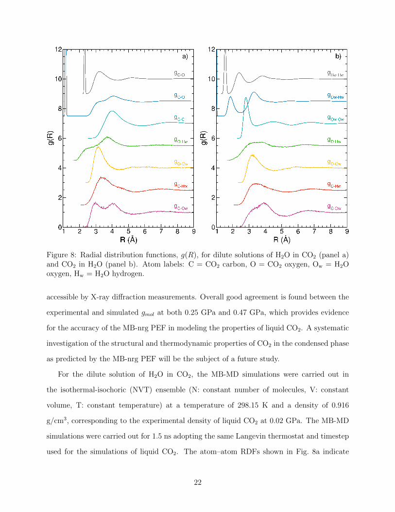
Figure 8: Radial distribution functions, g(R), for dilute solutions of H2O in CO2 (panel a)and CO2 in H2O (panel b). Atom labels: C = CO2 carbon, O = CO2 oxygen, Ow = H2Ooxygen, Hw = H2O hydrogen.
accessible by X-ray diffraction measurements. Overall good agreement is found between the
experimental and simulated gmol at both 0.25 GPa and 0.47 GPa, which provides evidence
for the accuracy of the MB-nrg PEF in modeling the properties of liquid CO2. A systematic
investigation of the structural and thermodynamic properties of CO2 in the condensed phase
as predicted by the MB-nrg PEF will be the subject of a future study.
For the dilute solution of H2O in CO2, the MB-MD simulations were carried out in
the isothermal-isochoric (NVT) ensemble (N: constant number of molecules, V: constant
volume, T: constant temperature) at a temperature of 298.15 K and a density of 0.916
g/cm3, corresponding to the experimental density of liquid CO2 at 0.02 GPa. The MB-MD
simulations were carried out for 1.5 ns adopting the same Langevin thermostat and timestep
used for the simulations of liquid CO2. The atom–atom RDFs shown in Fig. 8a indicate
22

significant structural reorganization of the CO2 molecules around the H2O molecule, which
can be better characterized from the analysis of the two distinct peaks in the CO2 carbon–
H2O oxygen (C-Ow) RDF. Specifically, the first peak at ∼3.0 A corresponds to configurations
in which the C atom of a CO2 molecule interacts with the O atom of the water molecule
while the second peak at ∼4.0 A corresponds to configurations in which the water molecule
forms hydrogen bonds with the O atoms of the surrounding CO2 molecules. The formation
of hydrogen bonds between H2O and the surrounding CO2 molecules is further confirmed by
the presence of the shoulder at ∼2.2 A in the O–Hw RDF.
For the dilute solution of CO2 in H2O, the MB-MD simulations were carried out for
680 ps in the NVT ensemble at a temperature of 298.15 K and a density of 0.997 g/cm3,
which corresponds to the experimental density of liquid water at 1 atm, using the same
Langevin thermostat and timestep as for neat liquid CO2 and H2O in CO2. The atom–atom
RDFs shown in Fig. 8b indicate the structure of liquid water remains largely unperturbed
by the presence of the CO2 molecule. This can be easily explained by considering the
difference in interaction strengths between the CO2–H2O (-2.961 kcal/mol) and H2O–H2O (-
4.952 kcal/mol)62 dimers, with the latter dominating and largely favoring hydrogen bonding
between water molecules. This is manifested in the absence of the two distinct peaks in the
C-Ow) RDF and the shoulder at ∼2.2 A in the O–Hw RDF.
Overall, the MB-nrg simulated RDFs shown in Figs. 8 for both dilute solutions of H2O in
CO2 and CO2 in H2O are in qualitative agreement with the corresponding RDFs calculated
in Ref. 50 using a molecular model specifically optimized to reproduce the properties of
CO2/H2O liquid mixtures. A detailed analysis of CO2/H2O liquid mixtures as a function of
temperature, pressure, and mole fractions will be the subject of a forthcoming publication.
23

4 Conclusions
In this study, we have introduced many-body PEFs for neat CO2 and mixed CO2/H2O sys-
tems developed within the TTM-nrg68,70 and MB-nrg69,71 frameworks. While both TTM-nrg
and MB-nrg PEFs build upon the MB-pol PEF for water,62–64 and adopt the same functional
forms to describe permanent electrostatics, polarization, and dispersion, they differ in the
representation of short-range contributions, with the TTM-nrg PEFs relying on conventional
Born-Mayer expressions and the MB-nrg PEFs employing multidimensional permutationally
invariant polynomials.
The accuracy of the TTM-nrg and MB-nrg PEFs has been assessed through a systematic
analysis of the interaction and many-body energies calculated for (CO2)m(H2O)n clusters,
with m+n ≤ 4, as well as through comparisons with available experimental data for the CO2-
CO2 and CO2-H2O second virial coefficients and structural properties of various CO2/H2O
liquid mixtures. Our analysis demonstrates that the MB-nrg PEFs quantitatively reproduce
reference data obtained at the coupled cluster level of theory, the current “gold standard”
for molecular interactions,122 without relying on error cancellation and correctly predict
both gas- and liquid-phase properties. As for the MB-nrg PEFs describing the interactions
of halide68,69 and alkali-metal ions70,71 with water, the level of accuracy achieved by the
MB-nrg PEFs for neat CO2 and mixed CO2/H2O systems can be traced back to their ability
to correctly represent individual many-body contributions to the interaction energies.
Future studies will focus on the characterization of the phase behavior of CO2/H2O
fluid mixtures as a function of temperature, pressure, and composition, in the bulk and
in confinement as well as on the extension of the MB-nrg framework to the modeling of
multicomponent systems of arbitrary (small) molecules.
24

5 Supplementary Material
Tables listing all parameters of the TTM-nrg PEFs for CO2, CO2–CO2 and CO2–H2O, as well
as all distances and associated ξ variables used in the permutationally invariant polynomials
of the corresponding MB-nrg PEFs.
6 Acknowledgements
The authors thank Dr. Sandra Brown for his help with the training set generation and valu-
able discussions, Dr. Sandeep Reddy for his help with the implementation of the TTM-nrg
PEFs in our software, and Eleftherios Lambros for his help in the implementation of the
virial tensor calculation in MBX. This research was supported by the U.S. Department of
Energy, Office of Science, Office of Basic Energy Science through grant no. DE-SC0019490.
M.R.R. was supported by a Software Fellowship from the Molecular Sciences Software Insti-
tute, which is funded by the U.S. National Science Foundation (grant no. ACI-1547580). All
calculations for the training set generation were performed using resources provided by the
Open Science Grid,123,124 which is supported by the U.S. National Science Foundation and
the U.S. Department of Energy’s Office of Science. We thank Edgar Fajardo for his help and
technical support on the use of the software in the grid, and the Physics Computing Facili-
ties of the University of California, San Diego, for granting us access to the grid. The DFT
calculations used resources of the Extreme Science and Engineering Discovery Environment
(XSEDE), which is supported by the National Science Foundation (grant no. ACI-1548562)
as well as at the Triton Shared Computing Cluster (TSCC) at the San Diego Supercomputer
Center.
25

References
(1) Falkowski, P.; Scholes, R.; Boyle, E.; Canadell, J.; Canfield, D.; Elser, J.; Gruber, N.;
Hibbard, K.; Hogberg, P.; Linder, S., et al. The Global Carbon Cycle: A Test of Our
Knowledge of Earth as a System. Science 2000, 290, 291–296.
(2) Seinfeld, J. H.; Pandis, S. N. Atmospheric Chemistry and Physics: From Air Pollution
to Climate Change; John Wiley & Sons, 2016.
(3) Butler, J. N. Carbon Dioxide Equilibria and Their Applications ; Routledge, 2019.
(4) Caldeira, K.; Wickett, M. E. Oceanography: Anthropogenic Carbon and Ocean pH.
Nature 2003, 425, 365.
(5) Sabine, C. L.; Feely, R. A.; Gruber, N.; Key, R. M.; Lee, K.; Bullister, J. L.; Wan-
ninkhof, R.; Wong, C.; Wallace, D. W.; Tilbrook, B., et al. The Oceanic Sink for
Anthropogenic CO2. Science 2004, 305, 367–371.
(6) Fleyfel, F.; Devlin, J. P. Carbon Dioxide Clathrate Hydrate Epitaxial Growth: Spec-
troscopic Evidence for Formation of the Simple Type-II Carbon Dioxide Hydrate. J.
Phys. Chem. 1991, 95, 3811–3815.
(7) Amthor, J. Respiration in a Future, Higher-CO2 World. Plant Cell Environ. 1991, 14,
13–20.
(8) Blankenship, R. E. Molecular Mechanisms of Photosynthesis ; John Wiley & Sons,
2014.
(9) Raupach, M. R.; Marland, G.; Ciais, P.; Le Quere, C.; Canadell, J. G.; Klepper, G.;
Field, C. B. Global and Regional Drivers of Accelerating CO2 Emissions. Proc. Natl.
Acad. Sci. U.S.A. 2007, 104, 10288–10293.
(10) Sakakura, T.; Choi, J.-C.; Yasuda, H. Transformation of Carbon Dioxide. Chem. Rev.
2007, 107, 2365–2387.
26

(11) Costentin, C.; Robert, M.; Saveant, J.-M. Catalysis of the Electrochemical Reduction
of Carbon Dioxide. Chem. Soc. Rev. 2013, 42, 2423–2436.
(12) James, J.; Thomas, P.; Cavan, D.; Kerr, D. Preventing Childhood Obesity by Reduc-
ing Consumption of Carbonated Drinks: Cluster Randomised Controlled Trial. BMJ
2004, 328, 1237.
(13) Hyatt, J. A. Liquid and Supercritical Carbon Dioxide as Organic Solvents. J. Org.
Chem. 1984, 49, 5097–5101.
(14) DeSimone, J. M. Practical Approaches to Green Solvents. Science 2002, 297, 799–803.
(15) Blunt, M.; Fayers, F. J.; Orr Jr, F. M. Carbon Dioxide in Enhanced Oil Recovery.
Energy Convers. Manag. 1993, 34, 1197–1204.
(16) Jacobs, G. K.; Kerrick, D. M. Methane: An Equation of State with Application to the
Ternary System H2O-CO2-CH4. Geochim. Cosmochim. Acta 1981, 45, 607–614.
(17) Bowers, T. S.; Helgeson, H. C. Calculation of the Thermodynamic and Geochemical
Consequences of Nonideal Mixing in the System H2O–CO2–NaCl on Phase Relations
in Geologic Systems: Equation of State for H2O–CO2–NaCl Fluids at High Pressures
and Temperatures. Geochim. Cosmochim. Acta 1983, 47, 1247–1275.
(18) Duan, Z.; Møller, N.; Weare, J. H. An Equation of State for the CH4–CO2–H2O
System: I. Pure Systems from 0 to 1000 C and 0 to 8000 Bar. Geochim. Cosmochim.
Acta 1992, 56, 2605–2617.
(19) Duan, Z.; Møller, N.; Weare, J. H. An Equation of State for the CH4–CO2–H2O
System: II. Mixtures from 50 to 1000 C and 0 to 1000 Bar. Geochim. Cosmochim.
Acta 1992, 56, 2619–2631.
(20) Pitzer, K. S.; Sterner, S. M. Equations of State Valid Continuously from Zero to
Extreme Pressures for H2O and CO2. J. Chem. Phys. 1994, 101, 3111–3116.
27

(21) Duan, Z.; Møller, N.; Weare, J. H. Equation of State for the NaCl–H2O–CO2 System:
Prediction of Phase Equilibria and Volumetric Properties. Geochim. Cosmochim. Acta
1995, 59, 2869–2882.
(22) Bakker, R. J. Adaptation of the Bowers and Helgeson (1983) Equation of State to the
H2O–CO2–CH4–N2–NaCl System. Chem. Geol. 1999, 154, 225–236.
(23) Duan, Z.; Zhang, Z. Equation of State of the H2O, CO2, and H2O–CO2 Systems up
to 10 GPa and 2573.15 K: Molecular Dynamics Simulations with Ab Initio Potential
Surface. Geochim. Cosmochim. Acta 2006, 70, 2311–2324.
(24) Mannik, L.; Stryland, J.; Welsh, H. An Infrared Spectrum of CO2 Dimers in the”
Locked” Configuration. Can. J. Phys. 1971, 49, 3056–3057.
(25) Seitz, J. C.; Pasteris, J. D.; Wopenka, B. Characterization of CO2–CH4–H2O Fluid In-
clusions by Microthermometry and Laser Raman Microprobe Spectroscopy: Inferences
for Clathrate and Fluid Equilibria. Geochim. Cosmochim. Acta 1987, 51, 1651–1664.
(26) Barnes, J.; Gough, T. Fourier Transform Infrared Spectroscopy of Molecular Clusters:
The Structure and Internal Mobility of Clustered Carbon Dioxide. J. Chem. Phys.
1987, 86, 6012–6017.
(27) Barth, H.-D.; Huisken, F. Investigation of Librational Motions in Gas-Phase CO2
Clusters by Coherent Raman Spectroscopy. Chem. Phys. Lett. 1990, 169, 198–203.
(28) Disselkamp, R.; Ewing, G. E. Large CO2 Clusters Studied by Infrared Spectroscopy
and Light Scattering. J. Chem. Phys. 1993, 99, 2439–2448.
(29) Olijnyk, H.; Jephcoat, A. Vibrational Studies on CO2 up to 40 GPa by Raman Spec-
troscopy at Room Temperature. Phys. Rev. B 1998, 57, 879.
(30) Yoon, J.-H.; Kawamura, T.; Yamamoto, Y.; Komai, T. Transformation of Methane
28

Hydrate to Carbon Dioxide Hydrate: In situ Raman Spectroscopic Observations. J.
Phys. Chem. A 2004, 108, 5057–5059.
(31) Tassaing, T.; Oparin, R.; Danten, Y.; Besnard, M. Water–CO2 Interaction in Su-
percritical CO2 as Studied by Infrared Spectroscopy and Vibrational Frequency Shift
Calculations. J. Supercrit. Fluids 2005, 33, 85–92.
(32) Lalanne, P.; Tassaing, T.; Danten, Y.; Cansell, F.; Tucker, S.; Besnard, M. CO−2
Ethanol Interaction Studied by Vibrational Spectroscopy in Supercritical CO2. J.
Phys. Chem. A 2004, 108, 2617–2624.
(33) Brinzer, T.; Berquist, E. J.; Ren, Z.; Dutta, S.; Johnson, C. A.; Krisher, C. S.; Lam-
brecht, D. S.; Garrett-Roe, S. Ultrafast Vibrational Spectroscopy (2D-IR) of CO2 in
Ionic Liquids: Carbon Capture from Carbon Dioxide’s Point of View. J. Chem. Phys.
2015, 142, 212425.
(34) Giammanco, C. H.; Kramer, P. L.; Yamada, S. A.; Nishida, J.; Tamimi, A.;
Fayer, M. D. Carbon Dioxide in an Ionic Liquid: Structural and Rotational Dynamics.
J. Chem. Phys. 2016, 144, 104506.
(35) Datchi, F.; Weck, G.; Saitta, A.; Raza, Z.; Garbarino, G.; Ninet, S.; Spaulding, D.;
Queyroux, J.; Mezouar, M. Structure of Liquid Carbon Dioxide at Pressures up to 10
GPa. Phys. Rev. B 2016, 94, 014201.
(36) Murthy, C.; O’Shea, S.; McDonald, I. Electrostatic Interactions in Molecular Crystals:
Lattice Dynamics of Solid Nitrogen and Carbon Dioxide. Mol. Phys. 1983, 50, 531–
541.
(37) Harris, J. G.; Yung, K. H. Carbon Dioxide’s Liquid–Vapor Coexistence Curve and
Critical Properties as Predicted by a Simple Molecular Model. J. Phys. Chem. 1995,
99, 12021–12024.
29

(38) Potoff, J.; Errington, J.; Panagiotopoulos, A. Z. Molecular Simulation of Phase Equi-
libria for Mixtures of Polar and Non-Polar Components. Mol. Phys. 1999, 97, 1073–
1083.
(39) Bukowski, R.; Sadlej, J.; Jeziorski, B.; Jankowski, P.; Szalewicz, K.; Kucharski, S. A.;
Williams, H. L.; Rice, B. M. Intermolecular Potential of Carbon Dioxide Dimer from
Symmetry-Adapted Perturbation Theory. J. Chem. Phys. 1999, 110, 3785–3803.
(40) Potoff, J. J.; Siepmann, J. I. Vapor–Liquid Equilibria of Mixtures Containing Alkanes,
Carbon Dioxide, and Nitrogen. AIChE J. 2001, 47, 1676–1682.
(41) Chialvo, A.; Houssa, M.; Cummings, P. Molecular Dynamics Study of the Structure
and Thermophysical Properties of Model SI Clathrate Hydrates. J. Phys. Chem. B
2002, 106, 442–451.
(42) Chatzis, G.; Samios, J. Binary Mixtures of Supercritical Carbon Dioxide with
Methanol. A Molecular Dynamics Simulation Study. Chem. Phys. Lett. 2003, 374,
187–193.
(43) Costa Gomes, M. F.; Padua, A. A. Interactions of Carbon Dioxide with Liquid Fluo-
rocarbons. J. Phys. Chem. B 2003, 107, 14020–14024.
(44) Zhang, Z.; Duan, Z. An Optimized Molecular Potential for Carbon Dioxide. J. Chem.
Phys. 2005, 122, 214507.
(45) Geng, C.-Y.; Wen, H.; Zhou, H. Molecular Simulation of the Potential of Methane
Reoccupation during the Replacement of Methane Hydrate by CO2. J. Phys. Chem.
A 2009, 113, 5463–5469.
(46) Makarewicz, J. Intermolecular Potential Energy Surface of the Water–Carbon Dioxide
Complex. J. Chem. Phys. 2010, 132, 234305.
30

(47) Qi, Y.; Ota, M.; Zhang, H. Molecular Dynamics Simulation of Replacement of CH4 in
Hydrate with CO2. Energy Convers. Manag. 2011, 52, 2682–2687.
(48) Herri, J.-M.; Bouchemoua, A.; Kwaterski, M.; Fezoua, A.; Ouabbas, Y.; Cameirao, A.
Gas Hydrate Equilibria for CO2–N2 and CO2–CH4 Gas Mixtures–Experimental Stud-
ies and Thermodynamic Modelling. Fluid Ph. Equilibria 2011, 301, 171–190.
(49) Wheatley, R. J.; Harvey, A. H. Intermolecular Potential Energy Surface and Second
Virial Coefficients for the Water–CO2 Dimer. J. Chem. Phys. 2011, 134, 134309.
(50) Vlcek, L.; Chialvo, A. A.; Cole, D. R. Optimized Unlike-Pair Interactions for Water–
Carbon Dioxide Mixtures Described by the SPC/E and EPM2 Models. J. Phys. Chem.
B 2011, 115, 8775–8784.
(51) Yu, K.; McDaniel, J. G.; Schmidt, J. Physically Motivated, Robust, Ab Initio Force
Fields for CO2 and N2. J. Phys. Chem. B 2011, 115, 10054–10063.
(52) Yu, K.; Schmidt, J. Many-Body Effects Are Essential in a Physically Motivated CO2
Force Field. J. Chem. Phys. 2012, 136, 034503.
(53) Moultos, O. A.; Tsimpanogiannis, I. N.; Panagiotopoulos, A. Z.; Economou, I. G.
Atomistic Molecular Dynamics Simulations of CO2 Diffusivity in H2O for a Wide
Range of Temperatures and Pressures. J. Phys. Chem. B 2014, 118, 5532–5541.
(54) Orozco, G. A.; Economou, I. G.; Panagiotopoulos, A. Z. Optimization of Intermolec-
ular Potential Parameters for the CO2/H2O Mixture. J. Phys. Chem. B 2014, 118,
11504–11511.
(55) Jiang, H.; Moultos, O. A.; Economou, I. G.; Panagiotopoulos, A. Z. Gaussian-Charge
Polarizable and Nonpolarizable Models for CO2. J. Phys. Chem. B 2016, 120, 984–
994.
31

(56) Jiang, H.; Economou, I. G.; Panagiotopoulos, A. Z. Phase Equilibria of Water/CO2
and Water/n-Alkane Mixtures from Polarizable Models. J. Phys. Chem. B 2017, 121,
1386–1395.
(57) Wang, Q.; Bowman, J. M. Two-Component, Ab Initio Potential Energy Surface for
CO2–H2O, Extension to the Hydrate Clathrate, CO2@(H2O)20, and VSCF/VCI Vi-
brational Analyses of Both. J. Chem. Phys. 2017, 147, 161714.
(58) Sode, O.; Cherry, J. N. Development of a Flexible-Monomer Two-Body Carbon Diox-
ide Potential and Its Application to Clusters up to (CO2)13. J. Comp. Chem. 2017,
38, 2763–2774.
(59) Bukowski, R.; Szalewicz, K.; Groenenboom, G. C.; Van der Avoird, A. Predictions of
the Properties of Water from First Principles. Science 2007, 315, 1249–1252.
(60) Wang, Y.; Shepler, B. C.; Braams, B. J.; Bowman, J. M. Full-Dimensional, Ab Initio
Potential Energy and Dipole Moment Surfaces for Water. J. Chem. Phys. 2009, 131,
054511.
(61) Wang, Y.; Huang, X.; Shepler, B. C.; Braams, B. J.; Bowman, J. M. Flexible, Ab
Initio Potential, and Dipole Moment Surfaces for Water. I. Tests and Applications for
Clusters up to the 22-mer. J. Chem. Phys. 2011, 134, 094509.
(62) Babin, V.; Leforestier, C.; Paesani, F. Development of a “First Principles” Water
Potential with Flexible Monomers: Dimer Potential Energy Surface, VRT Spectrum,
and Second Virial Coefficient. J. Chem. Theory Comput. 2013, 9, 5395–5403.
(63) Babin, V.; Medders, G. R.; Paesani, F. Development of a “First Principles” Water
Potential with Flexible monomers. II: Trimer Potential Energy Surface, Third Virial
Coefficient, and Small Clusters. J. Chem. Theory Comput. 2014, 10, 1599–1607.
32

(64) Medders, G. R.; Babin, V.; Paesani, F. Development of a “First-Principles” Water
Potential with Flexible Monomers. III. Liquid Phase Properties. J. Chem. Theory
Comput. 2014, 10, 2906–2910.
(65) Pinski, P.; Csanyi, G. Reactive Many-Body Expansion for a Protonated Water Cluster.
J. Chem. Theory Comput. 2013, 10, 68–75.
(66) Conte, R.; Qu, C.; Bowman, J. M. Permutationally Invariant Fitting of Many-Body,
Non-Covalent Interactions with Application to Three-Body Methane–Water–Water.
J. Chem. Theory Comput. 2015, 11, 1631–1638.
(67) Yu, Q.; Bowman, J. M. Ab Initio Potential for H3O+→ H+ + H2O: A Step to a Many-
Body Representation of the Hydrated Proton? J. Chem. Theory Comput. 2016, 12,
5284–5292.
(68) Arismendi-Arrieta, D. J.; Riera, M.; Bajaj, P.; Prosmiti, R.; Paesani, F. i-TTM Model
for Ab Initio-Based Ion–Water Interaction Potentials. 1. Halide–Water Potential En-
ergy Functions. J. Phys. Chem. B 2015, 120, 1822–1832.
(69) Bajaj, P.; Gotz, A. W.; Paesani, F. Toward Chemical Accuracy in the Description of
Ion–Water Interactions through Many-Body Representations. I. Halide–Water Dimer
Potential Energy Surfaces. J. Chem. Theory Comput. 2016, 12, 2698–2705.
(70) Riera, M.; Gotz, A. W.; Paesani, F. The i-TTM Model for Ab Initio-Based Ion–Water
Interaction Potentials. II. Alkali Metal Ion–Water Potential Energy Functions. Phys.
Chem. Chem. Phys. 2016, 18, 30334–30343.
(71) Riera, M.; Mardirossian, N.; Bajaj, P.; Gotz, A. W.; Paesani, F. Toward Chemical
Accuracy in the Description of Ion–Water Interactions through Many-Body Represen-
tations. Alkali-Water Dimer Potential Energy Surfaces. J. Chem. Phys. 2017, 147,
161715.
33

(72) Yu, Q.; Bowman, J. M. Communication: VSCF/VCI Vibrational Spectroscopy of
H7O3 ∗ + and H9O+4 using High-Level, Many-Body Potential Energy Surface and
Dipole Moment Surfaces. J. Chem. Phys. 2017, 146, 121102.
(73) Qu, C.; Bowman, J. M. A Fragmented, Permutationally Invariant Polynomial Ap-
proach for Potential Energy Surfaces of Large Molecules: Application to N-Methyl
Acetamide. J. Chem. Phys. 2019, 150, 141101.
(74) Paesani, F. Getting the Right Answers for the Right Reasons: Toward Predictive
Molecular Simulations of Water with Many-Body Potential Energy Functions. Acc.
Chem. Res. 2016, 49, 1844–1851.
(75) Reddy, S. K.; Straight, S. C.; Bajaj, P.; Huy Pham, C.; Riera, M.; Moberg, D. R.;
Morales, M. A.; Knight, C.; Gotz, A. W.; Paesani, F. On the Accuracy of the MB-pol
Many-Body Potential for Water: Interaction Energies, Vibrational Frequencies, and
Classical Thermodynamic and Dynamical Properties from Clusters to Liquid Water
and Ice. J. Chem. Phys. 2016, 145, 194504.
(76) Mardirossian, N.; Head-Gordon, M. ω B97M-V: A Combinatorially Optimized, Range-
Separated Hybrid, Meta-GGA Density Functional with VV10 Nonlocal Correlation.
J. Chem. Phys. 2016, 144, 214110.
(77) Mayer, J.; Goeppert-Mayer, M. Statistical Mechanics ; John Wiley & Sons, New York,
1940.
(78) Hankins, D.; Moskowitz, J.; Stillinger, F. Water Molecule Interactions. J. Chem. Phys.
1970, 53, 4544–4554.
(79) Bajaj, P.; Wang, X.-G.; Carrington Jr, T.; Paesani, F. Vibrational Spectra of Halide–
Water Dimers: Insights on Ion Hydration from Full-Dimensional Quantum Calcula-
tions on Many-Body Potential Energy Surfaces. J. Chem. Phys. 2018, 148, 102321.
34

(80) Riera, M.; Brown, S. E.; Paesani, F. Isomeric Equilibria, Nuclear Quantum Effects,
and Vibrational Spectra of M+ (H2O) n= 1–3 Clusters, with M= Li, Na, K, Rb, and
Cs, through Many-Body Representations. J. Phys. Chem. A 2018, 122, 5811–5821.
(81) Bizzarro, B. B.; Egan, C. K.; Paesani, F. Nature of Halide–Water Interactions: Insights
from Many-Body Representations and Density Functional Theory. J. Chem. Theory
Comput. 2019, 15, 2983–2995.
(82) Paesani, F.; Bajaj, P.; Riera, M. Chemical Accuracy in Modeling Halide Ion Hydration
from Many-Body Representations. Adv. Phys. X 2019, 4, 1631212.
(83) Bajaj, P.; Richardson, J. O.; Paesani, F. Ion-Mediated Hydrogen-Bond Rearrangement
through Tunnelling in the Iodide–Dihydrate Complex. Nat. Chem. 2019, 11, 367.
(84) Bajaj, P.; Zhuang, D.; Paesani, F. Specific Ion Effects on Hydrogen-Bond Rearrange-
ments in the Halide–Dihydrate Complexes. J. Phys. Chem. Lett. 2019, 10, 2823–2828.
(85) Bajaj, P.; Riera, M.; Lin, J. K.; Mendoza Montijo, Y. E.; Gazca, J.; Paesani, F. Halide
Ion Microhydration: Structure, Energetics, and Spectroscopy of Small Halide–Water
Clusters. J. Phys. Chem. A 2019, 123, 2843–2852.
(86) Zhuang, D.; Riera, M.; Schenter, G. K.; Fulton, J. L.; Paesani, F. Many-Body Effects
Determine the Local Hydration Structure of Cs+ in Solution. J. Phys. Chem. Lett.
2019, 10, 406–412.
(87) Braams, B. J.; Bowman, J. M. Permutationally Invariant Potential Energy Surfaces
in High Dimensionality. Int. Rev. Phys. Chem. 2009, 28, 577–606.
(88) Burnham, C.; Anick, D.; Mankoo, P.; Reiter, G. The Vibrational Proton Potential in
Bulk Liquid Water and Ice. J. Chem. Phys. 2008, 128, 154519.
(89) Stone, A. The Theory of Intermolecular Forces ; Oxford University Press, Oxford,
2013.
35

(90) Tang, K.; Toennies, J. P. An Improved Simple Model for the van der Waals Potential
Based on Universal Damping Functions for the Dispersion Coefficients. J. Chem. Phys.
1984, 80, 3726–3741.
(91) Brown, S. E.; Georgescu, I.; Mandelshtam, V. A. Self-Consistent Phonons Revisited.
II. A General and Efficient Method for Computing Free Energies and Vibrational
Spectra of Molecules and Clusters. J. Chem. Phys. 2013, 138, 044317.
(92) Tihonov, A. N. Solution of Incorrectly Formulated Problems and the Regularization
Method. Soviet Math. 1963, 4, 1035–1038.
(93) Breneman, C. M.; Wiberg, K. B. Determining Atom-Centered Monopoles from Molec-
ular Electrostatic Potentials. The Need for High Sampling Density in Formamide Con-
formational Analysis. J. Comp. Chem. 1990, 11, 361–373.
(94) Shao, Y.; Gan, Z.; Epifanovsky, E.; Gilbert, A. T. B.; Wormit, M.; Kussmann, J.;
Lange, A. W.; Behn, A.; Deng, J.; Feng, X.; Ghosh, D.; Goldey, M.; Horn, P. R.; Jacob-
son, L. D.; Kaliman, I.; Khaliullin, R. Z.; Kus, T.; Landau, A.; Liu, J.; Proynov, E. I.;
Rhee, Y. M.; Richard, R. M.; Rohrdanz, M. A.; Steele, R. P.; Sundstrom, E. J.; Wood-
cock III, H. L.; Zimmerman, P. M.; Zuev, D.; Albrecht, B.; Alguire, E.; Austin, B.;
Beran, G. J. O.; Bernard, Y. A.; Berquist, E.; Brandhorst, K.; Bravaya, K. B.;
Brown, S. T.; Casanova, D.; Chang, C.-M.; Chen, Y.; Chien, S. H.; Closser, K. D.;
Crittenden, D. L.; Diedenhofen, M.; DiStasio Jr., R. A.; Dop, H.; Dutoi, A. D.;
Edgar, R. G.; Fatehi, S.; Fusti-Molnar, L.; Ghysels, A.; Golubeva-Zadorozhnaya, A.;
Gomes, J.; Hanson-Heine, M. W. D.; Harbach, P. H. P.; Hauser, A. W.; Hohen-
stein, E. G.; Holden, Z. C.; Jagau, T.-C.; Ji, H.; Kaduk, B.; Khistyaev, K.; Kim, J.;
Kim, J.; King, R. A.; Klunzinger, P.; Kosenkov, D.; Kowalczyk, T.; Krauter, C. M.;
Lao, K. U.; Laurent, A.; Lawler, K. V.; Levchenko, S. V.; Lin, C. Y.; Liu, F.;
Livshits, E.; Lochan, R. C.; Luenser, A.; Manohar, P.; Manzer, S. F.; Mao, S.-P.;
Mardirossian, N.; Marenich, A. V.; Maurer, S. A.; Mayhall, N. J.; Oana, C. M.;
36
Olivares-Amaya, R.; O’Neill, D. P.; Parkhill, J. A.; Perrine, T. M.; Peverati, R.;
Pieniazek, P. A.; Prociuk, A.; Rehn, D. R.; Rosta, E.; Russ, N. J.; Sergueev, N.;
Sharada, S. M.; Sharmaa, S.; Small, D. W.; Sodt, A.; Stein, T.; Stuck, D.; Su, Y.-C.;
Thom, A. J. W.; Tsuchimochi, T.; Vogt, L.; Vydrov, O.; Wang, T.; Watson, M. A.;
Wenzel, J.; White, A.; Williams, C. F.; Vanovschi, V.; Yeganeh, S.; Yost, S. R.;
You, Z.-Q.; Zhang, I. Y.; Zhang, X.; Zhou, Y.; Brooks, B. R.; Chan, G. K. L.;
Chipman, D. M.; Cramer, C. J.; Goddard III, W. A.; Gordon, M. S.; Hehre, W. J.;
Klamt, A.; Schaefer III, H. F.; Schmidt, M. W.; Sherrill, C. D.; Truhlar, D. G.;
Warshel, A.; Xua, X.; Aspuru-Guzik, A.; Baer, R.; Bell, A. T.; Besley, N. A.;
Chai, J.-D.; Dreuw, A.; Dunietz, B. D.; Furlani, T. R.; Gwaltney, S. R.; Hsu, C.-
P.; Jung, Y.; Kong, J.; Lambrecht, D. S.; Liang, W.; Ochsenfeld, C.; Rassolov, V. A.;
Slipchenko, L. V.; Subotnik, J. E.; Van Voorhis, T.; Herbert, J. M.; Krylov, A. I.;
Gill, P. M. W.; Head-Gordon, M. Advances in molecular quantum chemistry con-
tained in the Q-Chem 4 program package. Mol. Phys. 2015, 113, 184–215.
(95) Dunning Jr, T. H. Gaussian Basis Sets for Use in Correlated Molecular Calculations. I.
The Atoms Boron through Neon and Hydrogen. J. Chem. Phys. 1989, 90, 1007–1023.
(96) Kendall, R. A.; Dunning Jr, T. H.; Harrison, R. J. Electron Affinities of the First-Row
Atoms Revisited. Systematic Basis Sets and Wave Functions. J. Chem. Phys. 1992,
96, 6796–6806.
(97) Woon, D. E.; Dunning Jr, T. H. Gaussian Basis Sets for Use in Correlated Molecular
Calculations. III. The Atoms Aluminum through Argon. J. Chem. Phys. 1993, 98,
1358–1371.
(98) Woon, D. E.; Dunning Jr, T. H. Gaussian Basis Sets for Use in Correlated Molecular
Calculations. IV. Calculation of Static Electrical Response Properties. J. Chem. Phys.
1994, 100, 2975–2988.
37

(99) Woon, D. E.; Dunning Jr, T. H. Gaussian Basis Sets for Use in Correlated Molecular
Calculations. V. Core-Valence Basis Sets for Boron through Neon. J. Chem. Phys.
1995, 103, 4572–4585.
(100) Becke, A. D.; Johnson, E. R. Exchange-Hole Dipole Moment and the Dispersion In-
teraction. J. Chem. Phys. 2005, 122, 154104.
(101) Johnson, E. R.; Becke, A. D. A Post-Hartree–Fock Model of Intermolecular Interac-
tions. J. Chem. Phys. 2005, 123, 024101.
(102) Johnson, E. R.; Becke, A. D. A Post-Hartree-Fock Model of Intermolecular Interac-
tions: Inclusion of Higher-Order Corrections. J. Chem. Phys. 2006, 124, 174104.
(103) Adler, T. B.; Knizia, G.; Werner, H. J. A Simple and Efficient CCSD(T)-F12 Approx-
imation. J. Chem. Phys. 2007, 127, 221106.
(104) Knizia, G.; Adler, T. B.; Werner, H.-J. Simplified CCSD (T)-F12 Methods: Theory
and Benchmarks. J. Chem. Phys. 2009, 130, 054104.
(105) Hill, J. G.; Peterson, K. A.; Knizia, G.; Werner, H.-J. Extrapolating MP2 and CCSD
Explicitly Correlated Correlation Energies to the Complete Basis Set Limit with First
and Second Row Correlation Consistent Basis Sets. J. Chem. Phys. 2009, 131, 194105.
(106) Gora, U.; Podeszwa, R.; Cencek, W.; Szalewicz, K. Interaction Energies of Large
Clusters from Many-Body Expansion. J. Chem. Phys. 2011, 135, 224102.
(107) Boys, S. F.; Bernardi, F. The Calculation of Small Molecular Interactions by the
Differences of Separate Total Energies. Some Procedures with Reduced Errors. Mol.
Phys. 1970, 19, 553–566.
(108) Werner, H.-J.; Knowles, P.; Knizia, G.; Manby, R.; Schutz, M.; et al., MOLPRO,
Version 2012.1, A Package of Ab Initio Programs. 2012; see http://www.molpro.net.
38

(109) Medders, G. R.; Babin, V.; Paesani, F. A Critical Assessment of Two-Body and Three-
Body Interactions in Water. J. Chem. Theory Comput. 2013, 9, 1103–1114.
(110) Medders, G. R.; Gotz, A. W.; Morales, M. A.; Bajaj, P.; Paesani, F. On the Repre-
sentation of Many-Body Interactions in Water. J. Chem. Phys. 2015, 143, 104102.
(111) Riera, M.; Lambros, E.; Nguyen, T.; Goetz, A.; Paesani, F. Low-Order Many-Body
Interactions Determine the Local Structure of Liquid Water. Chem Sci. 2019, 10,
8211–8218.
(112) Paesani, F. Water: Many-Body Potential from First Principles (From the Gas to
the Liquid Phase). Handbook of Materials Modeling: Methods: Theory and Modeling
2018, 1–25.
(113) Jmol: An Open-Source Java Viewer for Chemical Structures in 3D.
http://www.jmol.org/, Version 13.0.
(114) Holste, J.; Hall, K.; Eubank, P.; Esper, G.; Watson, M.; Warowny, W.; Bailey, D.;
Young, J.; Bellomy, M. Experimental (p, Vm, T) for Pure CO2 between 220 and 450
K. J. Chem. Thermodyn. 1987, 19, 1233–1250.
(115) Patel, M. R.; Joffrion, L. L.; Eubank, P. T. A Simple Procedure for Estimating Virial
Coefficients from Burnett PVT Data. AIChE J. 1988, 34, 1229–1232.
(116) Duschek, W.; Kleinrahm, R.; Wagner, W. Measurement and Correlation of the (Pres-
sure, Density, Temperature) Relation of Carbon Dioxide I. The Homogeneous Gas and
Liquid Regions in the Temperature Range from 217 K to 340 K at Pressures up to 9
MPa. J. Chem. Thermodyn. 1990, 22, 827–840.
(117) Patel, M. R.; Holste, J. C.; Hall, K. R.; Eubank, P. T. Thermophysical Properties of
Gaseous Carbon Dioxide–Water Mixtures. Fluid Ph. Equilibria 1987, 36, 279–299.
39
(118) Meyer, C. W.; Harvey, A. H. Dew-Point Measurements for Water in Compressed
Carbon Dioxide. AIChE J. 2015, 61, 2913–2925.
(119) Medders, G. R.; Paesani, F. Infrared and Raman Spectroscopy of Liquid Water
through “First-Principles” Many-Body Molecular Dynamics. J. Chem. Theory Com-
put. 2015, 11, 1145–1154.
(120) MBX: A Many-Body Energy Calculator. http://paesanigroup.ucsd.edu/
software/mbx.html, Accessed: 2019-07-05.
(121) Kapil, V.; Rossi, M.; Marsalek, O.; Petraglia, R.; Litman, Y.; Spura, T.; Cheng, B.;
Cuzzocrea, A.; Meißner, R. H.; Wilkins, D. M., et al. i-PI 2.0: A Universal Force
Engine for Advanced Molecular Simulations. Comput. Phys. Commun. 2019, 236,
214–223.
(122) Rezac, J.; Hobza, P. Benchmark Calculations of Interaction Energies in Noncovalent
Complexes and Their Applications. Chem. Rev. 2016, 116, 5038–5071.
(123) Pordes, R.; Petravick, D.; Kramer, B.; Olson, D.; Livny, M.; Roy, A.; Avery, P.; Black-
burn, K.; Wenaus, T.; Wurthwein, F.; Foster, I.; Gardner, R.; Wilde, M.; Blatecky, A.;
McGee, J.; Quick, R. The Open Science Grid. J. Phys. Conf. Ser. 2007, 78, 012057.
(124) Sfiligoi, I.; Bradley, D. C.; Holzman, B.; Mhashilkar, P.; Padhi, S.; Wurthwein, F.
The Pilot Way to Grid Resources Using GlideinWMS. 2009 WRI World congress on
computer science and information engineering. 2009; pp 428–432.
40

TOC Figure
41

download fileview on ChemRxivmany-body_mixtures.pdf (3.97 MiB)

Supporting Information
Data-Driven Many-Body Models for Molecular
Fluids: CO2/H2O Mixtures as a Case Study
Marc Riera-Riambau,∗,† Eric P. Yeh,† and Francesco Paesani∗,†,‡,¶
†Department of Chemistry and Biochemistry, University of California San Diego
La Jolla, California 92093, United States
‡Materials Science and Engineering, University of California San Diego
La Jolla, California 92093, United States
¶San Diego Supercomputer Center, University of California San Diego
La Jolla, California 92093, United States
E-mail: [email protected]; [email protected]
1

1 TTM-nrg PEFs
As discussed in the main text, the 1B term of the TTM-nrg PEF for neat CO2 is expressed
as a sum of the two bond stretching energies (V bond) and the angle bending energy (V angle).
Each bond energy is described by a Morse potential, while the bending energy is represented
by a harmonic potential,
V 1B = V bond + V angle
V bond = De
(1− e−a(rCO1
−reqCO))2
+De
(1− e−a(rCO2
−reqCO))2
V angle = 12k(φ− φeq)2
(1)
The parameters for the Morse potential representing the bond stretching energies (V bond)
are De = 189.05 kcal/mol, reqCO = 1.16 A, and a = 2.57 A−1, while the parameters for the
harmonic potential representing the the bending energy (V angle) are k = 87.87 kcal/mol/rad
and φeq = 180.0 degrees.
The CO2 atomic charges and polarizabilities used to represent both permanent and in-
duced electrostatic contributions in the TTM-nrg PEFs for CO2–CO2 and CO2–H2O are
listed in Table 1.
Table 1: Atomic charges (q) and polarizabilities (αeff) for CO2.
Atom q αeff
C 0.706 1.47167O -0.353 0.76979
2

The parameters of the Born-Mayer functions used to represent the repulsive energy terms
in the TTM-nrg PEFs for CO2–CO2 and CO2–H2O dimers are listed in Tables 2 and 3,
respectively.
Table 2: Parameters for the TTM-nrg CO2–CO2 PEF.
Parameter Value Units
ACC 9038.48 kcal/molACO 12608.9 kcal/molAOO 24274.7 kcal/molbCC 3.12663 A−1
bCO 3.64236 A−1
bOO 3.52744 A−1
C6,CC 321.009 kcal/mol/A6
C6,CO 219.550 kcal/mol/A6
C6,OO 170.095 kcal/mol/A6
Table 3: Parameters for the TTM-nrg CO2–H2O PEF.
Parameter Value Units
ACOw 4735.44 kcal/molACHw 4956.27 kcal/molAOOw 30678.4 kcal/molAOHw 4559.97 kcal/molbCOw 2.93819 A−1
bCHw 3.73590 A−1
bOOw 3.53045 A−1
bOHw 3.89503 A−1
C6,COw 225.586 kcal/mol/A6
C6,CHw 130.845 kcal/mol/A6
C6,OOw 208.075 kcal/mol/A6
C6,OHw 94.1987 kcal/mol/A6
3

2 MB-nrg PEFs
The variables involved in the permutationally invariant polynomial representing the 1B term
of the MB-nrg PEF for CO2 are listed in Table 4. l
Table 4: Distances and corresponding ξi variables of the permutationally invariant polyno-mial representing the 1B CO2 MB-nrg PEF (V 1B
poly).
Distance Atom 1 Atom 2 Variable
d1 C O1 ξ1 = e−kCO(d1−dCO)
d2 C O2 ξ2 = e−kCO(d2−dCO)
d3 O1 O2 ξ3 = e−kOO(d3−dOO)
The variables involved in the permutationally invariant polynomial representing the 2B
terms of the MB-nrg CO2–CO2 and CO2–H2O PEFs are listed in Tables 5 and 6, respectively.
Table 5: Distances and corresponding ξi variables of the permutationally invariant polyno-mial representing the 2B MB-nrg CO2–CO2 PEF (V 2B
poly). The superscripts a and b denotethe two monomers, MA and MB, of the dimer.
Distance Atom 1 Atom 2 Variable
d1 Ca Oa1 ξ1 = e−kCOintra(d1−dCOintra)
d2 Ca Oa2 ξ2 = e−kCOintra(d2−dCOintra)
d3 Oa1 Oa
2 ξ3 = e−kOOintra(d3−dOOintra)
d4 Cb Ob1 ξ4 = e−kCOintra(d4−dCOintra)
d5 Cb Ob2 ξ5 = e−kCOintra(d5−dCOintra)
d6 Ob1 Ob
2 ξ6 = e−kOOintra(d6−dOOintra)
d7 Ca Cb ξ7 = e−kCC(d7−dCC)
d8 Ca Ob1 ξ8 = e−kCO(d8−dCO)
d9 Ca Ob2 ξ9 = e−kCO(d9−dCO)
d10 Oa1 Cb ξ10 = e−kCO(d10−dCC)
d11 Oa1 Ob
1 ξ11 = e−kOO(d11−dCO)
d12 Oa1 Ob
2 ξ12 = e−kOO(d12−dCO)
d13 Oa2 Cb ξ13 = e−kCO(d13−dCC)
d14 Oa2 Ob
1 ξ14 = e−kOO(d14−dCO)
d15 Oa2 Ob
2 ξ15 = e−kOO(d15−dCO)
4

Table 6: Distances and corresponding ξi variables of the permutationally invariant polyno-mial representing the 2B MB-nrg CO2–H2O PEF (V 2B
poly). The superscripts a and b denotethe two monomers, MA and MB, of the dimer.
Distance Atom 1 Atom 2 Variable
d1 Oa Ha1 ξ1 = e−kOHintra(d1−dOHintra)
d2 Oa Ha2 ξ2 = e−kOHintra(d2−dOHintra)
d3 Ha1 Ha
2 ξ3 = e−kHHintra(d3−dHHintra)
d4 Cb Ob1 ξ4 = e−kCOintra(d4−dCOintra)
d5 Cb Ob2 ξ5 = e−kCOintra(d5−dCOintra)
d6 Ob1 Ob
2 ξ6 = e−kOOintra(d6−dOOintra)
d7 Oa Cb ξ7 = e−kOwC(d7−dOwC)
d8 Oa Ob1 ξ8 = e−kOwO(d8−dOwO)
d9 Oa Ob2 ξ9 = e−kOwO(d9−dOwO)
d10 Ha1 Cb ξ10 = e−kHC(d10−dHC)
d11 Ha1 Ob
1 ξ11 = e−kHO(d11−dHO)
d12 Ha1 Ob
2 ξ12 = e−kHO(d12−dHO)
d13 Ha2 Cb ξ13 = e−kHC(d13−dHC)
d14 Ha2 Ob
1 ξ14 = e−kHO(d14−dHO)
d15 Ha2 Ob
2 ξ15 = e−kHO(d15−dHO)
d16 La1 Cb ξ16 = e−kLC(d16−dLC)
d17 La1 Ob
1 ξ17 = e−kLO(d17−dLO)
d18 La1 Ob
2 ξ18 = e−kLO(d18−dLO)
d19 La2 Cb ξ19 = e−kLC(d19−dLC)
d20 La2 Ob
1 ξ20 = e−kLO(d20−dLO)
d21 La2 Ob
2 ξ21 = e−kLO(d21−dLO)
5

download fileview on ChemRxivsupp_info.pdf (151.39 KiB)


download fileview on ChemRxivco2_h2o.pdf (266.17 KiB)