data driven regulation: theory and application to missing bids · menica, roger myerson, ariel...

Data Driven Regulation:

Theory and Application to Missing Bids

Sylvain Chassang

New York University

Kei Kawai

U.C. Berkeley

Jun Nakabayashi

Kindai University

Juan Ortner∗†

Boston University

March 15, 2019

Abstract

We document a novel bidding pattern observed in procurement auctions fromJapan: winning bids tend to be isolated. There is a missing mass of close losingbids. This pattern is suspicious in the following sense: it is inconsistent with compet-itive behavior under arbitrary information structures. Building on this observation,we develop a theory of data-driven regulation based on “safe tests,” i.e. tests thatare passed with probability one by competitive bidders, but need not be passed bynon-competitive ones. We provide a general class of safe tests exploiting weak equilib-rium conditions, and show that such tests reduce the set of equilibrium strategies thatcartels can use to sustain collusion. We provide an empirical exploration of varioussafe tests in our data, as well as discuss collusive rationales for missing bids.Keywords: missing bids, collusion, regulation, procurement.

∗Chassang: [email protected], Kawai: [email protected], Nakabayashi: [email protected],Ortner: [email protected].

†We are especially indebted to Steve Tadelis for encouragement and detailed feedback. The paper bene-fited from discussions with Pierpaolo Battigali, Eric Budish, Yeon-Koo Che, Francesco Decarolis, Emir Ka-menica, Roger Myerson, Ariel Pakes, Wolfgang Pesendorfer, Andrea Prat, Michael Riordan, Jozsef Sakovics,Larry Samuelson, Andy Skrzypacz, Paulo Somaini, as well as comments from seminar participants at the2018 ASSA meeting, the 2018 Canadian Economic Theory Conference, Bocconi, the 2017 Berkeley-Sorbonneworkshop on Organizational Economics, Boston University, Columbia University, EIEF, the 2018 ESSETmeeting at Gerzensee, FGV Rio, Harvard, HKUST, Johns Hopkins, MIT, NYU, the 2017 NYU CRATEconference on theory and econometrics, Penn State, Princeton, PUC Rio, Queen’s University, Rochester, the2018 Stanford SITE conference, Stanford GSB, the 2018 Transparency in Procurement Conference, TriangleMicroeconomics Conference, University of Arizona, University of Chicago, University of Copenhagen, Uni-versity of Illinois at Urbana-Champaign, UC Berkeley, University of Tokyo, University of Virginia, UCLA,and Yale.

1

1 Introduction

One of the key functions of antitrust authorities is to detect and punish collusion. Although

concrete evidence is required for successful prosecution, screening devices that flag suspicious

firm conduct may help regulators identify collusion, and encourage members of existing

cartels to apply for leniency programs. Correspondingly, an active research agenda has sought

to build data-driven methods to detect cartels using naturally occurring market data (e.g.

Porter, 1983, Porter and Zona, 1993, 1999, Ellison, 1994, Bajari and Ye, 2003, Harrington,

2008). This paper seeks to make progress on several questions relevant to this literature.

How should regulators act on data-driven evidence of collusion? Wouldn’t cartel members

adapt their play to the screening tests implemented by the regulator? If so, can we build

general tests that do not target only a specific pattern of behavior? Can we ensure that

regulatory policies do not end up strengthening cartels?

We begin by documenting a suspicious bidding pattern observed in procurement auctions

in Japan: the density of the bid distribution just above the winning bid is very low. There

is a missing mass of close losing bids. These missing bids are related to bidding patterns

of collusive firms in Hungary (Toth et al., 2014) and Switzerland (Imhof et al., 2016). We

establish that these missing bids indicate non-competitive behavior under a general class of

asymmetric information models, and under the presence of arbitrary unobserved heterogene-

ity. Indeed, this missing mass of bids makes it a profitable stage-game deviation for bidders

to increase their bids.

We expand on this observation and propose a theory of robust data-driven regulation

based on “safe tests,” i.e. tests that are passed with probability one by competitive bidders,

but not necessarily by non-competitive ones. We provide a general class of such tests ex-

ploiting weakened equilibrium conditions, and show that safe tests cannot help cartels: they

necessarily constrain the set of continuation values bidders can use to support collusion.

We illustrate the implications of various safe tests in our data, as well as propose several

2

explanations for why missing bids may arise as a by-product of collusion.

Our data come from two datasets of public works procurement auctions in Japan. The

first dataset, analyzed by Kawai and Nakabayashi (2018), contains data on approximately

78,000 national-level auctions held between 2001 and 2006 by the Ministry of Land, Infras-

tructure and Transportation. The second dataset, studied by Chassang and Ortner (forth-

coming), contains information on approximately 1,500 city-level auctions held between 2007

and 2014. We are interested in the distribution of bidders’ margins of victory (or defeat).

For every (bidder, auction) pair, we compute ∆, the difference between the bidder’s own bid

and the most competitive bid among this bidder’s opponents, divided by the reserve price.

When ∆ < 0, the bidder won the auction. When ∆ > 0 the bidder lost. The finding moti-

vating this paper is summarized by Figure 1, which plots the distribution of bid-differences

∆ in the sample of national-level auctions. There is a striking missing mass around ∆ = 0.

Our first goal is to clarify the sense in which this gap — and other patterns that could be

found in the data — are suspicious. Our second goal is to formulate a theory of regulatory

response to such data.

We analyze our data within a fairly general model of repeated play in first-price procure-

ment auctions. A group of firms repeatedly participates in first-price procurement auctions.

We allow players to observe arbitrary signals about one another, and rule out intertemporal

linkages between actions and payoffs. We allow bidders’ costs and types to be arbitrarily

correlated within and across periods. We say that behavior is competitive, if it is stage-game

optimal under the players’ information structure.

Our first set of results establishes that the pattern of missing bids illustrated in Figure

1 is not consistent with competitive behavior under any information structure. There is no

stochastic process for costs and types (ergodic or not) that would rationalize observed bids

in equilibrium. We exploit the fact that in any competitive equilibrium, firms must not find

it profitable in expectation to increase their bids. This incentive constraint implies that with

3

Figure 1: Distribution of bid-differences ∆ ≡ own bid−min(other bids)reserve

over (bidder, auction) pairsin national-level data.

high probability the elasticity of firms’ sample counterfactual demand (i.e., the empirical

probability of winning an auction at any given bid) must be bounded above by -1. This

condition is not satisfied in our data: because winning bids are isolated, the elasticity of

sample counterfactual demand is close to zero. In addition we are able to derive bounds on

the minimum number of histories at which non-competitive bidding must happen.

This empirical finding begs the question: what should a regulator do about it? If the

regulator investigates industries on the basis of such empirical evidence, won’t cartels adapt?

Could the regulator make collusion worse by reducing the welfare of competitive players?

Our second set of results formulates a theory of regulation based on safe tests. Like the

elasticity test described above, safe tests can be passed with probability one provided firms

are competitive under some information structure. We show how to exploit equilibrium

conditions to derive a large class of such tests. Finally, we show that regulatory policy based

on safe tests is a robust improvement over laissez-faire. Regulation based on safe tests cannot

hurt competitive bidders, and, provided penalties against colluding firms are large enough,

4

it can only reduce the set of enforceable collusive schemes available to cartels.

Our third set of results takes safe tests to the data. We delineate how different moment

conditions (i.e. different deviations) uncover different non-competitive patterns. In addition,

we show that the outcomes of our tests are consistent with other proxy evidence for compet-

itiveness and collusion. The sample of histories such that bids are close to the reserve price

is more likely to fail our tests than histories where bids are low relative to the reserve price.

Bidding histories before an industry is investigated for collusion are more likely to fail our

tests than bidding histories after being investigated for collusion. Altogether this suggests

that, although safe tests are conservative, they still have bite in practice.

Our paper relates primarily to the literature on cartel detection.1 Porter and Zona

(1993, 1999) show that suspected cartel members and non-cartel members bid in statistically

different ways. Bajari and Ye (2003) design a test of collusion based on excess correlation

across bids. Porter (1983) and Ellison (1994) exploit dynamic patterns of play predicted by

the theory of repeated games (Green and Porter, 1984, Rotemberg and Saloner, 1986) to

detect collusion. Conley and Decarolis (2016) propose a test of collusion in average-price

auctions exploiting cartel members’ incentives to coordinate bids. Chassang and Ortner

(forthcoming) propose a test of collusion based on changes in behavior around changes in

the auction design. Kawai and Nakabayashi (2018) analyze auctions with re-bidding, and

exploit correlation patterns in bids across stages to detect collusion.2 We propose a class of

robust, systematic tests of non-competitive behavior guaranteed to make cartel formation

less attractive in equilibrium.

A small set of papers study the equilibrium impact of data driven regulation. Cyrenne

(1999) and Harrington (2004) study repeated oligopoly models in which colluding firms might

get investigated and fined whenever prices exhibit large and rapid fluctuations.3 A common

1See Harrington (2008) for a recent survey.2Also related is Schurter (2017), who proposes a test of collusion based on exogenous shifts in the number

of bidders.3Other papers, like Besanko and Spulber (1989) and LaCasse (1995), study static models of equilibrium

regulation.

5

observation from these papers is that data driven regulation may backfire, allowing a cartel

to sustain higher equilibrium prices. We contribute to this literature by introducing the idea

of safe tests, and showing that regulation based on such tests restricts the set of equilibrium

values a cartel can sustain.

Our emphasis on safe tests connects our work to a branch of the microeconomic literature

that seeks to identify predictions that can be made for all underlying economic environments.

The work of Bergemann and Morris (2013) is particularly relevant: for a given finite game,

they study the range of behavior that can be sustained by some incomplete information

structure.4 A similar exercise is at the heart of our analysis, though we choose to consider

optimality conditions that are weaker and more easily satisfied than equilibrium. Our work

is also related to a branch of the mechanism design literature that considers endogenous

responses to collusion (Abdulkadiroglu and Chung, 2003, Che and Kim, 2006, Che et al.,

2018).

The tests that we propose, which seek to quantify violations of competitive behavior,

are similar in spirit to the tests used in revealed preference theory.5 Afriat (1967), Varian

(1990) and Echenique et al. (2011) propose tests to quantify the extent to which a given

consumption data set violates GARP. More closely related, Carvajal et al. (2013) propose

revealed preference tests of the Cournot model. We add to this literature by proposing tests

aimed at detecting non-competitive behavior in auctions which are robust to a wide range

of informational environments.

Finally, our paper makes an indirect contribution to the literature on the internal organi-

zation of cartels. Asker (2010) studies stamp auctions, and analyses the effect of a particular

collusive scheme on non-cartel bidders and sellers. Pesendorfer (2000) studies the bidding

4Also closely related is Bergemann et al. (2017), which characterizes bounds on equilibrium revenue infirst-price auctions under arbitrary incomplete information. Instead, we focus on implications for biddingbehavior under arbitrary incomplete information, and impose conditions that are weaker (and hence moreplausibly satisfied) than equilibrium. See also Doval and Ely (2019) for an extension allowing for arbitraryextensive form in addition to arbitrary incomplete information.

5See Chambers and Echenique (2016) for a recent review of the literature on revealed preference.

6

patterns for school milk contracts and compares the collusive schemes used by strong cartels

and weak cartels (i.e., cartels that used transfers and cartels that didn’t). Clark and Houde

(2013) document the collusive strategies used by the retail gasoline cartel in Quebec. Clark

et al. (2018) study the effect of an investigation on firms’ bidding behavior. We add to

this literature by documenting a puzzling bidding pattern that is poorly accounted for by

existing theories. We establish that this bidding pattern is non-competitive, and propose

some potential explanations.

The paper is structured as follows. Section 2 describes our data and documents missing

bids. Section 3 introduces our theoretical framework. Section 4 shows that missing bids

cannot be rationalized under any competitive model. Section 5 generalizes this analysis,

and provides safe tests that systematically exploit weak optimality conditions implied by

equilibrium. Section 6 proposes normative foundations for safe tests. Section 7 delineates

the mechanics of safe tests in real data, and shows that their implications are consistent

with other indicators of collusion. Section 8 concludes with an open ended discussion of why

missing bids may arise in the context of collusion. Appendix A reports descriptive statistics

of our data, as well as additional empirical results. Appendix B clarifies the connection

between our approach and Bayes correlated equilibrium (Bergemann and Morris, 2016).

Appendix C shows how our results extend under common values. Appendix D describes our

computational strategy. Proofs are collected in Appendix E unless mentioned otherwise.

2 Motivating Facts

Our first dataset, described in Kawai and Nakabayashi (2018), consists of roughly 78,000

auctions held between 2001 and 2006 by the Ministry of Land, Infrastructure and Trans-

portation in Japan (the Ministry). The auctions are sealed-bid first-price auctions with

a secret reserve price, and re-bidding in case there is no successful winner. The auctions

involve construction projects. The median winning bid is about 1 million USD, and the

7

median number of participants is 10. The bids of all participants are publicly revealed after

each auction.

For any given firm i participating in auction a with reserve price r, we denote by bi,a

the bid of firm i in auction a, and by b−i,a the profile of bids by bidders other than i. We

investigate the distribution of

∆i,a =bi,a − ∧b−i,a

r

aggregated over firms i, and auctions a, where ∧ denotes the minimum operator. The value

∆i,a represents the margin by which bidder i wins or loses auction a. If ∆i,a < 0 the bidder

won, if ∆i,a > 0 she lost.

The left panel of Figure 2 plots the distribution of bid differences ∆ aggregating over

all firms and auctions in our sample.6 The mass of missing bids around a difference of 0 is

starkly visible. This pattern can be traced to individual firms as well. The right panel of

Figure 2 reports the distribution of bid difference for a single large firm frequently active in

our sample of auctions.

(a) all firms (b) single large firm

Figure 2: Distribution of normalized bid-differences ∆ – national-level data.

Our second dataset, analyzed in Chassang and Ortner (forthcoming), consists of roughly

6Note that the distribution of normalized bid-differences is skewed to the right since the most competitivealternative bid is a minimum over other bidders’ bids.

8

1,500 auctions held between 2007 and 2014 by the city of Tsuchiura in Ibaraki prefecture,

also in Japan. Projects are allocated using a sealed-bid first-price auction with a public

reserve price. The median winning bid is about 130,000 USD, and the median number of

participants is 4. Figure 3 plots the distribution of ∆ for auctions held in Tsuchiura. Again,

we see a significant mass of missing bids around zero.7

Figure 3: Distribution of bid-difference ∆ – city data.

One key goal of the paper is to show that the bidding patterns illustrated in Figures 2

and 3 are inconsistent with competitive behavior under any information structure. While

this is different from saying that these patterns reflect collusive behavior, missing bids are

in fact correlated with plausible indicators of collusion.

Figure 4 breaks down the auctions in Figure 2 by bid levels: the figure plots the distri-

bution of ∆i,a =bi,a−∧b−i,a

rfor normalized bids

bi,ar

below 0.8 and above 0.8. The mass of

missing bids in Figure 2 is considerably reduced when we look at bids that are low compared

7Imhof et al. (2016) document a similar bidding pattern in procurement auctions in Switzerland: biddingpatterns by several cartels uncovered by the Swiss competition authority presented large differences betweenthe winning bid and the second lowest bid in auctions. See also Toth et al. (2014).

9

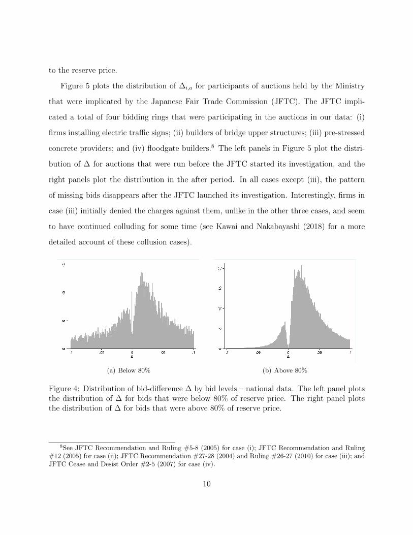
to the reserve price.

Figure 5 plots the distribution of ∆i,a for participants of auctions held by the Ministry

that were implicated by the Japanese Fair Trade Commission (JFTC). The JFTC impli-

cated a total of four bidding rings that were participating in the auctions in our data: (i)

firms installing electric traffic signs; (ii) builders of bridge upper structures; (iii) pre-stressed

concrete providers; and (iv) floodgate builders.8 The left panels in Figure 5 plot the distri-

bution of ∆ for auctions that were run before the JFTC started its investigation, and the

right panels plot the distribution in the after period. In all cases except (iii), the pattern

of missing bids disappears after the JFTC launched its investigation. Interestingly, firms in

case (iii) initially denied the charges against them, unlike in the other three cases, and seem

to have continued colluding for some time (see Kawai and Nakabayashi (2018) for a more

detailed account of these collusion cases).

(a) Below 80% (b) Above 80%

Figure 4: Distribution of bid-difference ∆ by bid levels – national data. The left panel plotsthe distribution of ∆ for bids that were below 80% of reserve price. The right panel plotsthe distribution of ∆ for bids that were above 80% of reserve price.

8See JFTC Recommendation and Ruling #5-8 (2005) for case (i); JFTC Recommendation and Ruling#12 (2005) for case (ii); JFTC Recommendation #27-28 (2004) and Ruling #26-27 (2010) for case (iii); andJFTC Cease and Desist Order #2-5 (2007) for case (iv).

10

Figure 5: Distribution of bid-difference ∆ – cartel cases in national data, before and afterJFTC investigation.

11

What does not explain this pattern. Although explaining missing bids is not the goal

of this paper, it is useful to clarify what does not explain this pattern. Specifically, we argue

that missing bids are not explained by either the granularity of bids, or ex post renegotiation.

Figures 4 and 5 rule out granularity as an explanation for missing bids: if missing bids

were a consequence of the granularity of bids, we should see similar patterns both across all

bid levels, and before and after the JFTC investigations.9

Renegotiation could potentially account for missing bids by making apparent incentive

compatibility issues irrelevant. Indeed, some winning firms may seemingly leave money on

the table, only to reclaim it through renegotiation ex post. Our national-level data contain

information on renegotiated prices, and allow us to rule out this explanation. First, Figure

6 shows that the missing bids pattern persists even if we focus on auctions whose prices

were not renegotiated up. Second, in the auctions we study, the contract that is signed

between the awarder and the awardee include renegotiation provisions that greatly reduce

firms’ incentives to bid aggressively with the hope of renegotiating to a higher price later on.

Specifically, the contract stipulates that renegotiated prices be anchored to the level of the

initial bid: if the project is estimated to cost $y more than initially thought, the renegotiated

price is increased by initial bidreserve price

× y. This implies that excessively competitive bids that are

unprofitable are likely to remain unprofitable after renegotiation.

Our objectives in this paper are: (i) to formalize why the missing mass of bids around zero

is suspicious; (ii) to delineate what it implies about bidding behavior and the competitiveness

of auctions in our sample; (iii) to formulate a theory of regulation based on safe tests; and

(iv) to propose possible explanations for why this behavior may arise under collusive bidding.

To do so we use a model of repeated auctions.

9In addition, there is no missing bid pattern when comparing the second and third lowest bids.

12

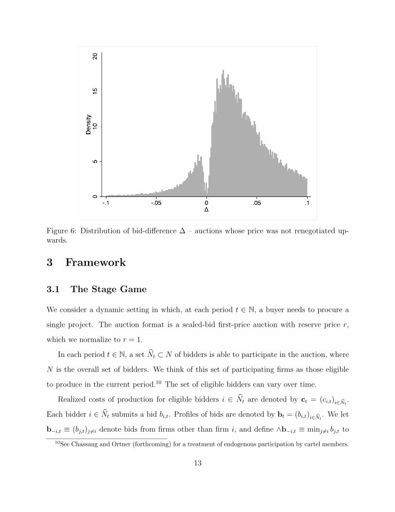
Figure 6: Distribution of bid-difference ∆ – auctions whose price was not renegotiated up-wards.

3 Framework

3.1 The Stage Game

We consider a dynamic setting in which, at each period t ∈ N, a buyer needs to procure a

single project. The auction format is a sealed-bid first-price auction with reserve price r,

which we normalize to r = 1.

In each period t ∈ N, a set Nt ⊂ N of bidders is able to participate in the auction, where

N is the overall set of bidders. We think of this set of participating firms as those eligible

to produce in the current period.10 The set of eligible bidders can vary over time.

Realized costs of production for eligible bidders i ∈ Nt are denoted by ct = (ci,t)i∈Nt.

Each bidder i ∈ Nt submits a bid bi,t. Profiles of bids are denoted by bt = (bi,t)i∈Nt. We let

b−i,t ≡ (bj,t)j 6=i denote bids from firms other than firm i, and define ∧b−i,t ≡ minj 6=i bj,t to

10See Chassang and Ortner (forthcoming) for a treatment of endogenous participation by cartel members.

13

be the lowest bid among i’s opponents at time t. The procurement contract is allocated to

the bidder submitting the lowest bid at a price equal to her bid. Ties are broken randomly.

Participants discount future payoffs using common discount factor δ < 1. Bids are

publicly revealed at the end of each period.11

Costs. We allow for costs that are serially correlated over time, and that may be correlated

across firms within each auction. Denoting by 〈., .〉 the usual dot-product we assume that

costs take the form

ci,t = 〈αi, θt〉+ εi,t > 0 (1)

where:12

• parameters αi ∈ Rk are fixed over time.

• θt ∈ Rk may be unknown to the bidders at the time of bidding, but is revealed to

bidders at the end of period t. We assume that θt follows a Markov chain.13 We do

not assume that there are finitely many states, or that the chain is irreducible.

• εi,t is i.i.d. with mean zero conditional on θt.

In period t, bidder i ∈ Nt obtains profits

πi,t = xi,t × (bi,t − ci,t),

where xi,t ∈ [0, 1] is the probability with which i wins the auction at time t. Note that costs

include both the direct costs of production and the opportunity cost of backlog.

11For the sake of concision, we do not consider the possibility of transfers at this point. It does not changeour analysis.

12We stress that cost specification (1) is flexible. For instance, this formulation can accommodate environ-ments in which costs depend on the physical distance between each firm i and the project’s location. Indeed,this can be achieved by setting θt to be the vector of distances from each firm to the project’s location attime t, and αi to be a vector with all zeros except a 1 in the i-th position.

13I.e. given any event E anterior to time t, θt|θt−1, E ∼ θt|θt−1.

14

The sets Nt of bidders are independent across time conditional on θt, i.e.

Nt|θt−1, Nt−1, Nt−2 . . . ∼ Nt|θt−1.

Information. In each period t, bidder i gets a signal zi,t that is conditionally i.i.d. given

(θt, (cj,t)j∈Nt). This allows our model to nest many informational environments, including

asymmetric information private value auctions, common value auctions, as well as complete

information. Bids bt are observable at the end of the auction.

3.2 Solution Concepts

A public history ht in period t takes the form ht = (θs−1,bs−1)s≤t. We let H denote the set

of all public histories.

Our solution concept is perfect public Bayesian equilibrium (Athey and Bagwell, 2008).

Because state θt is revealed at the end of each period, past play conveys no information about

the private types of other players. As a result we do not need to specify out-of-equilibrium

beliefs. A perfect public Bayesian equilibrium consists only of a strategy profile σ, such that

for all i ∈ N ,

σi : ht 7→ bi,t(zi,t),

where bids bi,t(zi,t) ∈ ∆([0, r]) depend on the public history and on the information available

at the time of decision making.

We emphasize the class of competitive equilibria, which simply corresponds to the class

of Markov perfect equilibria (Maskin and Tirole, 2001). In a competitive equilibrium, players

condition their play only on payoff relevant parameters.

Definition 1 (competitive strategy). We say that σ is competitive (or Markov perfect) if

and only if ∀i ∈ N and ∀ht ∈ H, σi(ht, zi,t) depends only on (θt−1, zi,t).

We say that a strategy profile σ is a competitive equilibrium if it is a perfect public

15

Bayesian equilibrium in competitive strategies.

We note that in a competitive equilibrium, firms must be playing a stage-game Nash

equilibrium at every period; that is, firms must play a static best-reply to the actions of

their opponents.

Competitive histories. Competitiveness of equilibrium is a fairly coarse notion. An

equilibrium, which could involve many firms, interacting over an extensive timeframe, is

either competitive or not. More realistically, an equilibrium may include periods in which

(a subset of) firms collude and periods in which firms compete. This leads us to define

competitive histories.

Definition 2 (competitive histories). Fix a common knowledge profile of play σ and a history

hi,t = (ht, zi,t) of player i. We say that player i is competitive at history hi,t if play at hi,t is

stage-game optimal for firm i given the behavior of other firms σ−i.

We say that a firm is competitive if it plays competitively at all histories on the equilibrium

path.

3.3 Safe Tests

We take the perspective of a regulator using bidding data to decide whether or not to launch

an investigation. We consider a regulator that seeks to do as little harm to competitive firms

as possible, and formalize her decision to intervene as a safe test. That is, a test that is

robustly passed by competitive firms. We show in Section 6 that preventing harm against

competitive firms serves an important strategic purpose: provided the cost of regulatory

intervention is high enough (at least for collusive firms), safe tests cannot unwittingly increase

a cartel’s enforcement capability. As Harrington (2004) highlights, this need not be true for

tests that are not safe.

16

Let H∞ denote the set of coherent full public histories (hi,t)i∈N,t≥0.14 A test τ is a mapping

from H∞ to 0, 1, where 1 denotes fail and 0 denotes pass.

Let us denote by λ ≡ prob((ci,t, θt, zi,t)i∈N,t≥0) the underlying economic environment, and

by Λ the set of possible environments λ.

Definition 3 (safe tests). We say that τi is unilaterally safe for firm i if and only if for all

λ ∈ Λ, and all profiles σ such that firm i is competitive, probλ,σ(τi(h) = 0) = 1.

We say that τ is jointly safe if and only if for all λ ∈ Λ, and all profiles σ such that all

players i ∈ N are competitive, probλ,σ(τ(h) = 0) = 1.

In words, a test is jointly safe (resp. unilaterally safe) if and only if all competitive

industries (resp. firms) pass the test with probability 1.

4 Missing Bids are Inconsistent with Competition

In this section, we show how to exploit equilibrium conditions at different histories to ob-

tain bounds on the share of competitive histories. The first step is to identify moments of

counterfactual demand that can be estimated from data, even though the subjective residual

demand faced by bidders can vary with the history.

4.1 Counterfactual demand

Fix a perfect public Bayesian equilibrium σ. For all histories hi,t and all bids b′ ∈ [0, r],

player i’s counterfactual demand at hi,t is

Di(b′|hi,t) ≡ probσ(∧b−i,t > b′|hi,t).

14I.e. sequences of histories such that hi,t and hi,t+1 coincide on events occurring before time t, andhi,t and hj,t+1 coincide on public events before t. For each each i ∈ N and t, history hi,t takes the formhi,t = (ht, zi,t).

17

For any finite set of histories H, and any scalar ρ ∈ (−1,∞), define

D(ρ|H) ≡ 1

|H|∑hi,t∈H

Di((1 + ρ)bi,t|hi,t)

the average counterfactual demand for histories in H, and its sample equivalent

D(ρ|H) ≡ 1

|H|∑hi,t∈H

1∧b−i,t>(1+ρ)bi,t .

Definition 4. We say that set of histories H is adapted to the players’ information if and

only if the event hi,t ∈ H is measurable with respect to player i’s information at time t prior

to bidding.

For instance, the set of auctions for a specific industry or location is adapted. In contrast,

the set of auctions in which the margin of victory is below a certain level is not. The ability

to legitimately vary the conditioning set H lets us explore the competitiveness of auctions

in particular settings of interest.

Lemma 1. Consider an adapted set of histories H. Under any perfect public Bayesian

equilibrium σ, for any α > 0,

prob(|D(ρ|H)−D(ρ|H)| ≤ α) ≥ 1− 2 exp(−α2|H|/2).

In particular, with probability 1, D(ρ|H)−D(ρ|H)→ 0 as |H| → ∞.

In other words, in equilibrium, the sample residual demand conditional on an adapted

set of histories converges to the true subjective aggregate conditional demand. This result

is a consequence of the equilibrium assumption, but is implied by optimality conditions

weaker than equilibrium. It may fail under sufficiently non-common priors, but will hold if

participants use data-driven predictors of demand satisfying no-regret (see for instance Hart

and Mas-Colell, 2000).

18

We highlight that Lemma 1 relies on conservative non-asymptotic concentration bounds.

In practice, one may be willing to make additional assumptions on the data generating

process leading to tighter estimates. Our approach extends to any probabilistic moment

conditions of the form

prob

((D(ρ|H)−D(ρ|H)

)ρ∈R∈ S

)≥ 1− ε

where R is a finite set of deviations ρ ∈ (−1,+∞), and S is a confidence set for demand

estimation errors D(ρ|H)−D(ρ|H) at different values of ρ ∈ R.15

4.2 A Test of Non-Competitive Behavior

The pattern of bids illustrated in Figures 1, 2 and 3 is striking. Our first main result shows

that its more extreme forms are inconsistent with competitive behavior.

Proposition 1. Let σ be a competitive equilibrium. Then,

∀hi,∂ logDi(b

′|hi)∂ log b′

∣∣b′=b+i (hi)

≤ −1, (2)

∀H, ∂ logD(ρ|H)

∂ρ∣∣ρ=0+

≤ −1. (3)

In words, under any competitive equilibrium, the elasticity of counterfactual demand

must be less than -1 at every history. The data presented in the left panel of Figure 2

contradicts the results in Proposition 1. Since the density of ∆i at 0 is essentially 0, the

elasticity of demand is approximately zero at these histories.

15For instance, if one is willing to impose that (θt)t∈N is stationary and ergodic, and that σ is a competitive

equilibrium, then D(ρ|H)−D(ρ|H) is asymptotically Gaussian when set H grows large. One can then deriveconfidence sets by estimating an asymptotic covariance matrix. Alternatively one may also derive confidencesets using bootstrap. This is the approach we use in our empirical analysis.

19

Proof. Consider a competitive equilibrium σ. Let

V (hi,t) ≡ Eσ

(∑s≥t

δs−t(bi,s − ci,s)1bi,s<∧b−i,s

∣∣hi,t)

denote player i’s discounted expected payoff at history hi,t. Let b denote the bid that bidder

i places at history hi,t. Since b is an equilibrium bid, it must be that for all bids b′ > b,

Eσ[(b− ci,t)1∧b−i,t>b + δV (hi,t+1)

∣∣hi,t, bi,t = b]

≥ Eσ[(b′ − ci,t)1∧b−i,t>b′ + δV (hi,t+1)

∣∣hi,t, bi,t = b′]

Since σ is competitive, Eσ[V (hi,t+1)|hi,t, bi,t = b] = Eσ[V (hi,t+1)|hi,t, bi,t = b′]. Hence, we must

have

bDi(b|hi,t)− b′Di(b′|hi,t) = Eσ

[b1∧b−i,t>b − b′1∧b−i,t>b′

∣∣hi,t]≥ Eσ

[ci,t(1∧b−i,t>b − 1∧b−i,t>b′)

∣∣hi,t] ≥ 0, (4)

where the last inequality follows since ci,t ≥ 0. Inequality (4) implies that, for all b′ > b,

logDi(b′|hi)− logDi(b|hi)

log b′ − log b≤ −1.

Inequality (2) follows from taking the limit as b′ → b. Inequality (3) follows from summing

(4) over histories in H, and performing the same computations.

As the proof highlights, this result exploits the fact that in procurement auctions, zero

is a natural lower bound for costs (see inequality (4)). In contrast, for auctions where

bidders have a positive value for the good, there is no corresponding natural upper bound to

valuations. One would need to impose an ad hoc upper bound on values to establish similar

results.

20

An implication of Proposition 1 is that, in our data, bidders have a short-term incentive

to increase their bids. Because of the need to keep participants from bidding higher, for

every ε > 0 small, there exists ν > 0 and a positive mass of histories hi,t = (ht, zi,t) such

that,

δEσ[V (hi,t+1)

∣∣hi,t, bi(hi,t)]− δEσ[V (hi,t+1)∣∣hi,t, bi(hi,t)(1 + ε)

]> ν. (5)

In other terms, equilibrium σ must give bidders a dynamic incentive not to overcut the

winning bid.

Proposition 1 proposes a simple test of whether an adapted dataset H can be generated

by a competitive equilibrium or not. Note that, unlike in tests of competitive behavior that

presume a particular information structure, the test here is valid under general information

structures including private values and common values. It is also valid under any form of

unobserved heterogeneity.16 We now refine this test to obtain bounds on the minimum share

of non-competitive histories needed to rationalize the data. We begin with a simple loose

bound and then propose a more sophisticated program resulting in tighter bounds.

4.3 Estimating the share of competitive histories

It follows from Proposition 1 that missing bids cannot be explained in a model of compet-

itive bidding. We now establish that competitive behavior must fail at a large number of

histories in order to explain isolated winning bids. This implies that bidders have frequent

opportunities to learn that their bids are not optimal.

Fix a perfect public Bayesian equilibrium σ and a finite set of histories H. Let Hcomp ⊂

H be the set of competitive histories in H. Define scomp ≡ |Hcomp||H| to be the fraction of

competitive histories in H. For all histories hi,t = (ht, zi,t) and all bids b′ ≥ 0, player i’s

16Since Proposition 1 holds conditional on the information that is available to firms, it must also holdconditional on the possibly coarser information available to the econometrician.

21

counterfactual revenue at hi,t is

Ri(b′|hi,t) ≡ b′Di(b

′|hi,t).

For any finite set of histories H and scalar ρ ∈ (−1,∞), define

R(ρ|H) ≡∑hi,t∈H

1

|H|(1 + ρ)bi,tDi((1 + ρ)bi,t|hi,t)

to be the average counterfactual revenue for histories in H. Our next result builds on

Proposition 1 to derive a bound on scomp.

Proposition 2. The share scomp of competitive histories is such that

scomp ≤ 1− supρ>0

R(ρ|H)−R(0|H)

ρ.

Proof. Let H¬comp = H\Hcomp be the set of non-competitive histories in H. For any ρ > 0,

1

ρ[R(ρ|H)−R(0|H)] = scomp

1

ρ

[R(ρ|Hcomp)−R(0|Hcomp)

]+ (1− scomp)

1

ρ

[R(ρ|H¬comp)−R(0|H¬comp)

]≤ 1− scomp.

The last inequality follows from two observations. First, since the elasticity of counterfactual

demand is bounded above by −1 for all competitive histories (Proposition 1), it follows that

R(ρ|Hcomp)−R(0|Hcomp) ≤ 0. Second, since R(ρ|H¬comp) ≤ (1 + ρ)R(0|H¬comp),

1

ρ[R(ρ|H¬comp)−R(0|H¬comp)] ≤ R(0|H¬comp) ≤ r = 1.

This concludes the proof.

22

In words, if total revenue for histories H increases by more than κ × ρ when bids are

uniformly increased by (1 + ρ), the share of competitive histories in H is bounded above by

1− κ.

Proposition 2 suggests a natural estimator. For each ρ ∈ (−1,∞), define

R(ρ|H) ≡∑hi,t∈H

1

|H|(1 + ρ)bi,t1∧b−i,t>(1+ρ)bi,t .

Note that R(ρ|H) is the sample analog of counterfactual revenue. A result identical to

Lemma 1 establishes that R(ρ|H) is a consistent estimator of R(ρ|H), whenever set H is

adapted. This allows us to use Proposition 2 to empirically estimate the share of competitive

histories.

In the extreme case where the density of competing bids is zero just above winning bids,

we have thatR(ρ|H)−R(0|H) ' ρR(0|H) for ρ small. This implies that scomp ≤ 1−R(0|H).17

While this bound is quite weak, we note that it is robust to private values, common values,

and any form of unobserved heterogeneity.

5 A General Class of Safe Tests

We now extend the approach of Section 4 to a derive a more general class of safe tests that

exploits the information content of both upward and downward deviations. We emphasize

that our tests allow the regulator or econometrician to include plausible constraints on costs,

incomplete information, and the extent of unobserved heterogeneity.

17Note that, since r = 1, scomp ≤ 1 − R(0|H) ≤ 1 −D(0|H). Hence, the bound on competitive historiesin Proposition 2 is, at most, equal to the probability of winning an auction.

23

5.1 A General Result

Take as given an adapted set of histories H, corresponding to a set A of auctions. Take as

given scalars ρn ∈ (−1,∞) for n ∈ M = −n, · · · , n, such that ρ0 = 0 and ρn < ρn′ for

all n′ > n. For each history hi,t ∈ H, let dhi,t,n ≡ Di((1 + ρn)bhi,t |hi,t). That is, dhi,t,n is

firm i’s subjective counterfactual demand at history hi,t, when applying a coefficient 1 + ρn

to its original bid. For any auction a and associated histories h ∈ a, an environment at a

is a tuple ωa = (dh,n, ch)h∈a, n∈M.18 We let ωA = (ωa)a∈A denote the profile of environments

across auctions a ∈ A.

For each deviation n, environment ωA = (ωa)a∈A and adapted set of histories H define

Dn(ωA, H) ≡ 1

|H|∑hi,t∈H

dhi,t,n and Dn(H) ≡ 1

|H|∑hi,t∈H

1(1+ρn)bhi,t<∧b−i,hi,t.

We formulate the problem of inference about the environment ωA as a constrained maxi-

mization problem defined by two objects to be chosen by the econometrician:

(i) u(ωa) the objective function to be maximized. For instance, the number of his-

tories h ∈ a that are rationalized as competitive under ωa.

(ii) Ω the set of plausible economic environments ωA.

Let U(ωA) =∑

a∈A u(ωa). For any tolerance function T : N → R+, we define inference

problem (P) as

U = maxωA∈Ω

U(ωA) (P)

s.t. ∀n, Dn(ωA, H) ∈[Dn(H)− T (|H|), Dn(H) + T (|H|)

]. (CR)

Intuitively, estimator U is a robust upper-bound to the true value U(ωA). It exploits the

18Note that for each history h ∈ H, there exists a corresponding bid placed by some bidder in an auctiona ∈ A. Hence, for the histories h ∈ a associated with auction a, our data contains the corresponding bidsplaced in auction a.

24

assumption that ωA is within the set of plausible environments Ω, as well as the fact that the

sample counterfactual demand aggregated over any set of adapted histories must converge

to the bidders’ expected counterfactual demand. We refer to this constraint as consistency

requirement (CR). The following result holds.

Proposition 3. Suppose the true environment is ωA ∈ Ω. Then, with probability at least

1− 2|M| exp(−1

2T (|H|)2|H|

), U ≥ U(ωA).

As we discussed following Lemma 1, any bound of the form

prob((D(ρn|H)−D(ρn|H))n∈M ∈ S) ≥ 1− ε

yields an extension of Proposition 3 where condition (CR) is replaced by (D(ρn|H) −

D(ρn|H))n∈M ∈ S. In that case, estimated metric U is greater than the true metric U(ωA)

with probability 1− ε.

We now show that by applying Proposition 3 to different tuples (u,Ω), we can derive

robust bounds on different measures of non-competitive behavior. These bounds imply

natural safe tests.

5.2 Maximum Share of Competitive Histories

We first use Proposition 3 to extend Proposition 2, and provide a tighter upper bound on

the share of competitive histories in H. For expositional purposes, we assume private values

and discuss extensions to common values at the end of this section.

Under the private values assumption, at every competitive history h ∈ H there must

25

exist costs ch and subjective demands dh = (dh,n)n∈M satisfying

feasibility: ch ∈ [0, bh]; ∀n, dh,n ∈ [0, 1]; ∀n, n′ > n, dh,n ≥ dh,n′ (F)

incentive compatibility: ∀n, [(1 + ρn)bh − ch] dh,n ≤ [(1 + ρ0)bh − ch]dh,0. (IC)

Conditions (F), (IC) and (CR) exploit some but not all the information content of equilib-

rium under some information structure. We clarify in Appendix B that this would be the

case if we imposed demand consistency requirements conditional on different values of bids

and costs c (corresponding to the bidder’s private information at the time of bidding).

The objective function u simply counts the number of histories satisfying these conditions:

u(ωa) ≡1

|H|∑h∈a∩H

1(dh,ch) satisfy (F) & (IC). (6)

We allow for economic plausibility constraints on environments Ω. We focus on markup

constraints, as well as constraints on the informativeness of signals bidders get.

∀h, bhch∈ [1 +m, 1 +M ] and ∀n,

∣∣∣∣logdh,n

1− dh,n− log

Dn

1−Dn

∣∣∣∣ ≤ k (EP)

where m ≥ 0 and M ∈ (m,+∞] are minimum and maximum markups, and k ∈ [0,+∞]

provides an upper bound to the information contained in any signal. The focal case of i.i.d.

types corresponds to k = 0.

For each environment ωA, define

Hcomp(ωA) ≡ h ∈ H s.t. (dh, ch) satisfy (F), (IC) and (EP)

to be the set of histories in H satisfying plausibility constraints (EP) that can be rationalized

26

as competitive under ωA. Program (P) then becomes

U = maxωA∈Ω

|Hcomp(ωA)||H|

(P′)


].

U provides an upper bound to the share of competitive histories in H, yielding the following

corollary.

Corollary 1. Suppose that the true environment ωA satisfies (EP), and that the true share

of competitive histories under environment ωA is scomp ∈ (0, 1]. Then, with probability at

least 1− 2|M| exp(−12T (|H|)2|H|), U ≥ scomp.

We note that, even when the deviations (ρn) are all upward deviations and we set m = 0,

M = ∞ and k = ∞, the bound Corollary 1 is still a tighter bound than the bound in

Proposition 2.19

The robust bound in Corollary 1 lets us define safe tests. For any threshold fraction

s0 ∈ (0, 1] of competitive histories, we define our candidate safe test by τ ≡ 1U≥s0 .

Corollary 2. Whenever T (·) satisfies lim|H|→∞ exp(−12T (|H|)2|H|) = 0, τ is a safe test.

By varying the initial set H of adapted histories, we can make test τ safe for a given

firm, or for a given industry. Specifically, if H is the set of histories of firm i, then test τ is

unilaterally safe for firm i.

For finite data, we can choose tolerance function T (·) to determine the significance level

of test τ . For instance, for the test to have a robust significance level of α ∈ (0, 1), we set

T (|H|) such that 2|M| exp(−12T (|H|)2|H|) = α. Note again that this is a very conservative

estimate of significance. One may obtain less conservative significance estimates by using

asymptotic concentration bounds tighter than the ones used to establish Lemma 1, or by

using bootstrap methods.

19Indeed, the bound in Proposition 2 uses the approximation R(0|H¬comp) ≤ 1, making it less tight thanthe bound in Corollary 1.

27

Common values. In the analysis above, the private value assumption implies that each

history h is associated with a single cost ch. Under common values, costs would depend on

the deviation ρ chosen by the bidder. An environment at auction a would then take the

form ωa = (dh,n, ch,n)h∈a, n∈M. However, we show in Appendix C that, under the assumption

that a bidder’s expected costs ch,n are weakly increasing in her opponents’ bids (a variant of

affiliation), common values cannot relax incentive compatibility constraint (IC). Hence, our

results extend without modification to such common value environments.

5.3 Bounds on Other Moments

Corollary 1 uses Proposition 3 to obtain bounds on the share of competitive histories. We

now show how to use Proposition 3 to bound other quantities of interest: the share of

competitive auctions, and the expected profits left on the table by non-optimizing bidders.

Maximum share of competitive auctions. The bound on the share of competitive

histories provided by Corollary 1 allows some histories in the same auctions to have dif-

ferent competitive/non-competitive status. This may underestimate the prevalence of non-

competition. In particular, if one player is non-competitive, she must expect other players

to be non-competitive in the future. Otherwise, if all of her opponents played competitively,

her stage-game best reply would be a profitable dynamic deviation.

For this reason we are interested in providing an upper bound on the share of competitive

auctions, where an auction is considered to be competitive if and only if every player is

competitive at their respective histories.

We define the objective function to be

u(ωa) =1

|A|1∀h∈a, (dh,ch) satisfy (F), (IC) & (EP)

For every environment ωA, let

28

Acomp(ωA) ≡ A′ ⊂ A s.t. ∀a ∈ A′,∀h ∈ a, (dh, ch) satisfy (F) (IC) & (EP).

be the set of competitive auctions under ωA. Program (P) then becomes

U = maxωA∈Ω

|Acomp(ωA)||A|


].

U provides an upper bound to the fraction of competitive auctions.

Total deviation temptation. Regulators may want to investigate an industry only if

firms fail to optimize in a significant way. Proposition 3 can be used to derive a lower bound

on the bidders’ deviation temptation. Given an environment ωa, we define objective

u(ωa) ≡1

|A|∑h∈a

[(bh − ch)dh,0 − max

n∈−n,··· ,n[(1 + ρn)bh − ch]dh,n

].

In this case, with large probability, −U is a lower bound for the average total deviation-

temptation per auction. This lets a regulator assess the extent of firms’ failure to optimize

before launching a costly audit. In addition, since the sum of deviation temptations must be

compensated by a share of the cartel’s future excess profits (along the lines of Levin (2003)),

U provides an indirect measure of the excess profits generated by the cartel.

6 Normative Foundations for Safe Tests

In this section we provide normative foundations for safe tests. We show that when pun-

ishments are severe enough, safe tests can be used to place constraints on potential cartel

members without creating new collusive equilibria.

29

A game of regulatory oversight. We study the equilibrium impact of data driven reg-

ulation within the following framework. From t = 0 to t =∞, firms in N play the infinitely

repeated game in Section 3. At t = ∞, after firms played the game, a regulator runs a

safe test on firms in N based on the realized history h∞ ∈ H∞. We consider two different

settings:

(i) The regulator runs a unilaterally safe test τi on each firm i ∈ N .

Firm i incurs an undiscounted penalty of K ≥ 0 if and only if τi(h∞) = 1 (i.e., if

and only if firm i fails the test).20

(ii) The regulator runs a jointly safe test τ on all firms in N .

Firms in N incur a penalty of K ≥ 0 if and only if τ(h∞) = 1.

When K = 0, under either form of testing the game collapses to the model of Section

3.21

Individually safe tests. For any K ≥ 0, let Σ(K) denote the set of perfect public

Bayesian equilibria of the game with firm-specific testing and with penalty K. Let K ≡ δ1−δ .

K serves as a rough upper bound on the difference in the continuation values a player obtains

for different actions.

Proposition 4 (safe tests do not create new equilibria). Assume the regulator runs unilat-

erally safe tests. For all K > K, Σ(K) ⊂ Σ(0).

When the penalty K is large enough (i.e., K > K), any equilibrium of the regulatory

game has the property that, at all histories (both on and off path), all firms expect to pass

the test with probability 1. Indeed, at every history, each firm can guarantee to pass the

test by playing a stage-game best reply at all future periods.

20Our analysis extends as is if K is the expected cost experienced by colluding firms from being investi-gated, while non-colluding firms experience a potentially lower cost.

21Since penalty K is undiscounted, the regulatory game is not continuous at infinity whenever K > 0.

30

Suppose K > K and fix σ ∈ Σ(K). Consider a public history ht, and let β = (βi)i∈N

be the bidding profile that firms use at ht under σ: for all i ∈ N , βi : zi 7→ R describes

firm i’s bid as a function of her signal. Let V = (Vi)i∈N be firms continuation payoffs

excluding penalties after history ht under σ, with Vi : b 7→ R mapping bids b = (bj)j∈N to

a continuation value for firm i. Bidding profile β must be such that, for all i ∈ N and all

possible signal realizations zi,

βi(zi) ∈ arg maxb

Eβ[(b− ci)1b<∧b−i+ δVi(b,b−i)|zi]− Eσ[τi|ht, b]K

=⇒βi(zi) ∈ arg maxb

Eβ[(b− ci)1b<∧b−i+ δVi(b,b−i)|zi],

where the second line follows since all firms pass the test with probability 1 after all histories.

In words, strategy profile σ is such that, at each history ht, no firm i has a profitable one

shot deviation in a game without testing. The one-shot deviation principle then implies that

σ ∈ Σ(0).22

Let ΣP (0) ⊂ Σ(0) denote the set of equilibria of the game without a regulator with the

property that, for all σ ∈ ΣP (0), all firms expect to pass the test with probability 1 at

every history. The arguments above imply that Σ(K) ⊂ ΣP (0) for all K > K. In fact, the

following stronger result holds:

Corollary 3. For all K > K, Σ(K) = ΣP (0).

We highlight that testing at the individual firm level is crucial for Proposition 4. Indeed,

as Cyrenne (1999) and Harrington (2004) show, regulation based on industry level tests may

backfire, allowing cartels to achieve higher equilibrium payoffs. Intuitively, when testing is at

the industry level, cartel members can punish deviators by playing a continuation strategy

that fails the test. This relaxes incentive constraints along the equilibrium path, and may

lead to more collusive outcomes.

22Note that the game with K = 0 is continuous at infinity, and so the one-shot deviation principle holdsin such game.

31

We note that although the set inclusion of Proposition 4 is weak, there are models of

bidder-optimal collusion such that the safe tests described in Section 5 strictly reduce the

surplus attainable by collusive bidders. We provide an explicit example in Section 8.

Jointly safe tests. An analogue of Proposition 4 holds for jointly safe test, provided we

impose Weak Renegotiation Proofness (see Farrell and Maskin, 1989).

Let Σ+RP (K) denote the set of Weakly Renegotiation Proof equilibria of the game with

joint testing and penalty K, such that all players get weakly positive expected discounted

payoffs in period 0. The following result holds.

Proposition 5. Assume the regulator runs a jointly safe test. For all K > K, Σ+RP (K) ⊂

Σ+RP (0).

Beyond safe tests. Sufficiently punitive safe tests do not make collusion more profitable,

and do not affect competitive industries. As a result, they should discourage the formation

of cartels. In contrast non-safe tests may increase cartel formation, either by reducing the

payoffs of competition, or enabling the cartel to sustain new collusive equilibria.

Still, a regulator with a strong prior may be willing to take some risks and implement

tests that are not safe, but very likely to lead to good outcomes under her prior. In this

sense, safe tests should be viewed as a starting point for regulation. Note that in our existing

framework, regulators may express some of their views on the underlying environment when

choosing the set of plausible economic environments Ω.

7 Empirical Evaluation

In this section, we explore the implications of our safe tests in real data. We argue that

safe tests tend not to fail when applied to data from likely competitive industries, and tend

to fail when applied to data from likely non-competitive industries. Details regarding the

32

computation of the tests are collected in Appendix D.

7.1 A Case Study

We first illustrate the mechanics of inference using data from the city of Tsuchiura.23 Specif-

ically, we show how three different deviations ρ ∈ −.02,−.0005, .0008 affect our estimates

of the share of competitive histories. The distribution of ∆ and the three deviations that we

consider are illustrated in Figure 7.

Figure 7: Distribution of ∆ for the city of Tsuchiura, 2007–2009. Red vertical lines indicatedeviation coefficients ρ ∈ −.02,−.0005, .0008.

Figure 8 presents our estimates of the 95% confidence bound on the share of competitive

histories as a function of the correlation parameter k in constraint (EP). For these estimates

and all the estimates that we present below, we use bootstrap to set tolerance T so that our

tests have a confidence level of 5%. We set values of the minimum and maximum markups

to m = 0.02 and M = 0.5. We now delineate the mechanics of inference.

23Chassang and Ortner (forthcoming) studies the impact of a change in the auction format used byTsuchiura that took place on October 29th 2009. We use data from auctions that took place before thatdate.

33

0.6 0.8 1.0 1.2 1.4 1.6 1.8 2.0k

0.0

0.2

0.4

0.6

0.8

1.0

shar

e of

com

petit

ive

hist

orie

s

Tsuchiura -- Share of Competitive Histories

upward dev.upward dev. and tiesupward, downward deviations and ties

Figure 8: Estimated share of competitive auctions, city-level data. Minimum and maximummarkups: m = 0.02,M = 0.25.

An upward deviation. We first consider a small upward deviation ρ = .0008, correspond-

ing to the analysis of Section 4. Because the mass of values of ∆ falling between 0 and .0008

is very small, this deviation hardly changes a bidder’s likelihood of winning an auction. As

a result this is a profitable deviation inconsistent with competition. Note that this upward

deviation is least profitable (and so the data is best explained) when costs are low.

Adding a small downward deviation. Consider next adding a small downward devia-

tion, ρ = −.0005. Because there is a surprisingly large mass of auctions such that the lowest

and second lowest bids are tied or extremely close, this increases a bidders likelihood of

winning by a non-vanishing amount, while reducing profits by a negligible amount, provided

margins are not zero. The corresponding histories cannot be competitive.

Adding a medium-sized downward deviation. We now show that, under certain con-

ditions, adding a medium sized downward deviation ρ = −.02 yields a tighter bound on

the share of competitive histories. Intuitively this is because the aggregate counterfactual

demand Dρ(H) increases by a large amount for relatively small deviations in bids: a 2%

34

drop in prices leads to a 44% increase in the probability of winning the auction. If costs of

production are sufficiently below bids, this is an attractive deviation.

7.2 Consistency between safe tests and proxies for collusion

We now turn to the national data to show that our estimates on the share of competi-

tive histories are consistent with different proxies of collusive behavior. For computational

tractability, we focus on estimating the share of competitive histories only using the three

deviations described above.

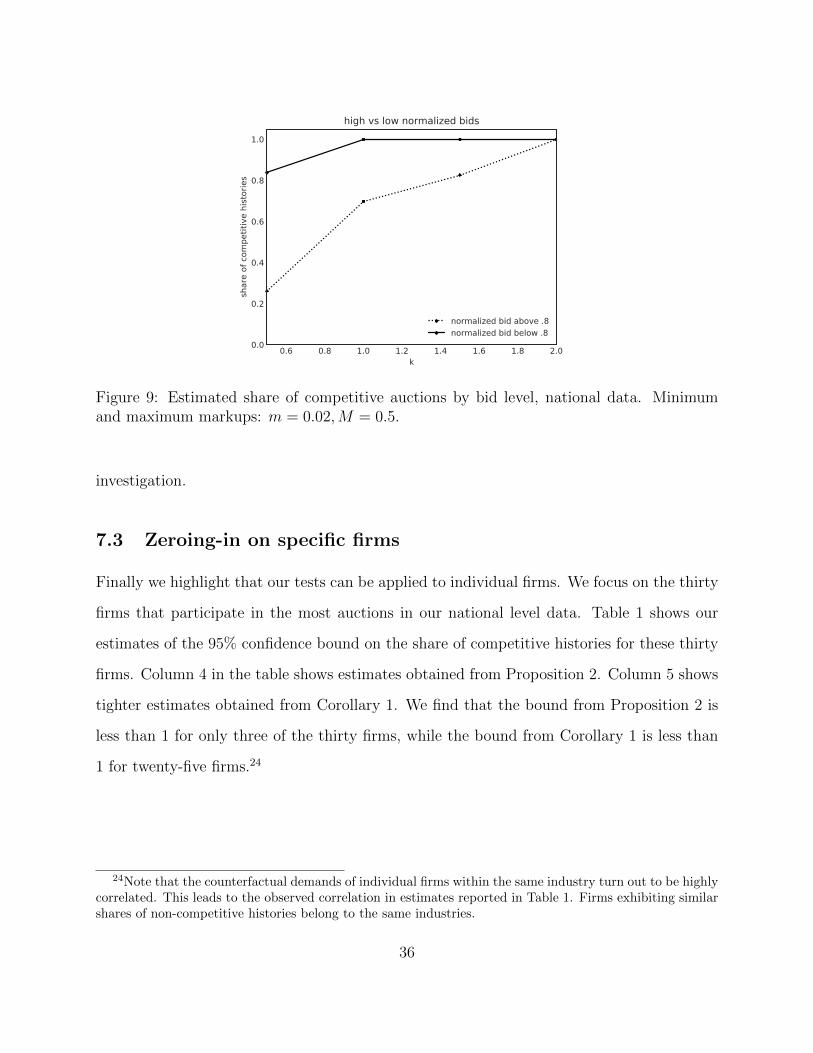
High vs. low bids. Figure 4 plots the distribution of ∆ for histories with high versus low

bid-to-reserve ratios (i.e., bids above/below 80% of the reserve price). The pattern of missing

bids is more striking when we focus on histories at which bidders place relatively high bids.

To the extent that missing bids are a marker of non-competitive behavior, Figure 4 suggests

that histories at which firms place relatively low bids are more likely to be competitive.

Figure 9 plots our estimates of the 95% confidence bound on the share of competitive

histories for the different sets of histories in Figure 4. For these results, we set the minimum

and maximum markups to m = 0.02 and M = 0.5. The fraction of competitive histories

is lower at histories at which bids are high relative to the reserve price, a finding that is

consistent with the idea that collusion is more likely for histories at which bidders place

higher bids.

Before and after prosecution. Figure 10 shows our estimates of the 95% confidence

bound on the share of competitive histories for the four groups of firms that were investigated

by the JFTC (see Section 2, and in particular Figure 5). Again, we use markup bounds

m = 0.02 and M = 0.5. Our estimates suggests non-competitive behavior in the before

period across the four groups of firms, and show a drop in non-competitive behavior following

35

0.6 0.8 1.0 1.2 1.4 1.6 1.8 2.0k

0.0

0.2

0.4

0.6

0.8

1.0

shar

e of

com

petit

ive

hist

orie

s

high vs low normalized bids

normalized bid above .8normalized bid below .8

Figure 9: Estimated share of competitive auctions by bid level, national data. Minimumand maximum markups: m = 0.02,M = 0.5.

investigation.

7.3 Zeroing-in on specific firms

Finally we highlight that our tests can be applied to individual firms. We focus on the thirty

firms that participate in the most auctions in our national level data. Table 1 shows our

estimates of the 95% confidence bound on the share of competitive histories for these thirty

firms. Column 4 in the table shows estimates obtained from Proposition 2. Column 5 shows

tighter estimates obtained from Corollary 1. We find that the bound from Proposition 2 is

less than 1 for only three of the thirty firms, while the bound from Corollary 1 is less than

1 for twenty-five firms.24

24Note that the counterfactual demands of individual firms within the same industry turn out to be highlycorrelated. This leads to the observed correlation in estimates reported in Table 1. Firms exhibiting similarshares of non-competitive histories belong to the same industries.

36

0.6 0.8 1.0 1.2 1.4 1.6 1.8 2.0k

0.0

0.2

0.4

0.6

0.8

1.0sh

are

of c

ompe

titiv

e hi

stor

ies

Electric

before investigationafter investigation

0.6 0.8 1.0 1.2 1.4 1.6 1.8 2.0k

0.0

0.2

0.4

0.6

0.8

1.0

shar

e of

com

petit

ive

hist

orie

s

Bridges


0.6 0.8 1.0 1.2 1.4 1.6 1.8 2.0k

0.0

0.2

0.4

0.6

0.8

1.0

shar

e of

com

petit

ive

hist

orie

s

Pre-Stressed Concrete


0.6 0.8 1.0 1.2 1.4 1.6 1.8 2.0k

0.0

0.2

0.4

0.6

0.8

1.0

shar

e of

com

petit

ive

hist

orie

s

Floods


Figure 10: Estimated share of competitive auctions, before and after FTC investigation,national-level data. Minimum and maximum markups: m = 0.02,M = 0.5.

8 Why Would Cartels Exhibit Missing Bids?

This paper focuses on the detection of non-competitive behavior in procurement auctions.

As we argue in Section 6 the robust detection of non-competitive behavior allows for data-

driven regulatory intervention that can only reduce the value of establishing a cartel. As

Section 7 highlights, the corresponding tests exploit the missing bid pattern, as well as other

aspects of the data: the large number of approximately tied bids, and the surprisingly large

elasticity of counterfactual demand to the left of winning bids.

We conclude with an open ended discussion of why missing bids may be occurring in

the first place. We argue that missing bids are not easily explained by standard models of

collusion, and put forward two potential explanations. Along the way we establish that safe

37

Ranking Participation Share won Share comp. (Prop. 2) Share comp. (Coro. 1)

1 4044 0.17 1.00 0.602 3854 0.07 1.00 0.683 3621 0.12 1.00 0.604 2998 0.15 1.00 1.005 2919 0.06 1.00 0.686 2547 0.08 1.00 0.157 2338 0.07 1.00 0.158 2333 0.07 1.00 0.189 2328 0.04 1.00 0.6810 2292 0.06 1.00 0.2011 2237 0.08 0.92 0.6812 2211 0.03 1.00 0.6813 2015 0.09 1.00 0.2814 1984 0.08 1.00 0.2815 1727 0.07 1.00 1.0016 1674 0.05 1.00 0.3117 1661 0.03 1.00 0.6818 1660 0.08 1.00 0.2819 1589 0.07 1.00 0.2820 1427 0.10 1.00 1.0021 1393 0.06 1.00 0.3122 1392 0.07 1.00 1.0023 1370 0.04 1.00 0.5624 1368 0.14 1.00 1.0025 1353 0.05 1.00 0.1626 1342 0.09 1.00 0.9127 1337 0.04 1.00 0.2528 1326 0.08 1.00 0.6029 1291 0.06 0.95 0.3130 1260 0.06 0.95 0.60

Table 1: Estimated Share of Competitive Auctions, National-Level Data. The table reportsour estimates of the share of competitive auctions for the thirty firms that participate inthe most number of auctions during the sample period. The first column corresponds to theranking of the firms and the second column corresponds to the number of auctions in whicheach firm participates. Column 3 shows the fraction of auctions that each of these firms wins.Columns 4 and 5 present our 95% confidence bound on the share of competitive histories foreach firm based on Proposition 2 and Corollary 1, respectively. For our estimates of columnfive, we use the following parameters: m = 0.02, M = 0.5 and k = 1.5.

38

tests can strictly reduce the surplus of cartels.

Standard models do not account for missing bids. In standard models of tacit col-

lusion (see for instance Rotemberg and Saloner (1986), Athey and Bagwell (2001, 2008)),

winning bids are typically common knowledge among bidders, and the cartel’s main concern

is to incentivize losers not to undercut the winning bid. In contrast, the behavior of the

designated winner is stage game optimal. This is achieved by having a losing bidder bid just

above the designated winner. As a consequence, standard models of collusion would result

in a point mass at ∆ = 0, rather than missing bids. If this were not the case, the cartel’s

pledgeable surplus would have to be spent on keeping the winner from increasing her bid

rather than keeping losing bidders from undercutting.

One implication of this is that there exist safe tests that strictly reduce the surplus of

cartels. Given a set of auctions A, consider tests that rule out frequent approximately-tied

winning bids:

τκ,ε(A) ≡

1 if |a ∈ A, s.t. b(2) − b(1) < κ|/|A| > ε

0 otherwise

where κ, ε > 0, and b(1), b(2) are the lowest and second lowest bids. Given ε > 0, conditional

on equilibrium markups being bounded away from 0, there exists κ small enough that τκ,ε is

a safe test under the assumption that competitive firms are privately informed about their

costs. This test fails the optimal collusive equilibria described above. In fact, such tests

are likely very highly powered: the probability that the lowest and second-lowest bids are

tied for a significant share auctions is likely very low under reasonable priors. This explains

why regulators use tied bids as an indicator of collusion (DOJ, 2005). It also suggests an

explanation for missing bids, as we now explain.

39

Missing bids as a side-effect of existing regulatory oversight. It is possible that

regulatory oversight itself may be at the origin of the missing bid pattern. Because test τκ,ε

is well powered with relatively small data sets, it makes sense for the regulator to scruti-

nize auctions in which tied bids occur. If this is the case, then collusive bidders sharing

information about their intended bids may naturally wish to avoid this scrutiny, and ensure

that there is a minimal distance between bids. Over many auctions, this may lead to the

detectable missing bids pattern highlighted in this paper.

Missing bids as robust coordination. Another possible role for missing bids consists

in facilitating coordination on a specific designated-winner. Being able to guarantee the

identity of the winner may be important for a cartel for two reasons: (i) allocative efficiency;

(ii) reducing the costs of dynamic incentive provision when utility is not transferable.

In this respect keeping winning bids isolated ensures that the designated winner does win

the contract, even if bidders cannot precisely agree on exact bids ex ante, or if bids can be

perturbed by small trembles (say a fat finger problem).

Online Appendix – Not for Publication

A Further Empirics

A.1 Sample Statistics

In this section we report descriptive statistics for our two illustrative datasets. At the auction

level, we report the mean and standard deviation of reserve prices, the lowest bid,25 the lowest

bid as a fraction of the reserve price, and the number of bidders participating in the auction.

At the bidder level, we report the mean and standard deviation of the number of auctions a

bidder participates in, the number of auctions she wins, and her total revenue.

We note that national-level auctions have higher reserve prices and a greater number

25This corresponds to the winning bid when the reserve price is public. If the reserve price is secret, thenthe lowest bid need not be the winning bid.

40

of participants, but the two datasets are nonetheless broadly comparable. We also note

that there is large heterogeneity in reserve prices in both cases, and in participation. Some

projects are very large, and some bidders participate very often.

N Mean S.D.

By Auctionsreserve price (mil. Yen) 78,272 105.121 259.58lowest first round bid (mil. Yen) 78,272 101.909 252.30lowest bid / reserve 78,272 0.970 0.10#bidders 78,272 9.883 2.27

By Biddersparticipation 29,670 26.40 94.61number of times lowest bidder 29,670 2.64 10.57total revenue (mil. Yen) 29,670 264.23 1312.77

Table A.1: Sample Statistics – National-Level Data

N Mean S.D.

By Auctionsreserve price (mil. Yen) 1,469 26.363 65.054lowest first round bid (mil. Yen) 1,469 24.749 61.745lowest bid / reserve 1,469 0.936 0.078#bidders 1,469 4.00 1.84

By Biddersparticipation 269 26.40 94.61number of times lowest bidder 269 5.803 9.240total revenue (mil. Yen) 269 167.342 447.014

Table A.2: Sample Statistics – City-Level Data

41

A.2 Total deviation temptation

In this section, we apply Proposition 3 to the objective function

u(ωa) ≡1

|H|∑h∈a

(bh − ch)dh,0 −maxn∈−n,··· ,n[(1 + ρn)bh − ch]dh,n(bh − ch)dh,0

.

This corresponds to firms’ minimum deviation temptation as a share of expected profits.

Figure A.1 reports estimates for firms in our city-level data.

0.2 0.4 0.6 0.8 1.0 1.2 1.4k

0.000

0.005

0.010

0.015

0.020

0.025

0.030

devi

atio

n te

mpt

atio

n as

a sh

are

of p

rofit

s

Tsuchiura -- Deviation Gain

before minimum price

Figure A.1: Estimated total deviation temptation as a fraction of profits, city-level data.Minimum and maximum markups: m = 0.02,M = 0.5.

B Connection with Bayes Correlated Equilibrium

In this section we further extend the class of estimators and tests introduced Section 5 and

clarify what would need to be added so that they exploit all implications from equilibrium.

This allows us to connect with the work of Bergemann and Morris (2016).

For simplicity we assume that player identities i, bids b and costs c take a fixed finite

number of values (i, b, c) ∈ I×B×C that does not grow with sample size. Ties between bids

are resolved with uniform probability. Deviations ρn ∈ (−1,∞) correspond to the ratios of

different bids on finite grid B.

We extend problem (P) as follows. As in Section 5.2, the objective function counts

42

whether a history is competitive or not:

u(ωa) ≡1

|H|∑h∈a∩H

1(dh,ch) satisfy (F) & (IC) and U(ωA) =∑a∈A

u(ωa).

For any (i, b, c) ∈ I × B × C, let us define Hi,b,c(ωA) ≡ h ∈ H|(ih, bh, ch) = (i, b, c),histories at which bidder i experiences a cost c and bids b. Note that Hi,b,c is adapted to the

information of player i. For any tolerance function T : N→ R+ such that

limN→∞

T (N) = 0 and limN→∞

exp

(−1

2T (N)2N

)= 0

we consider inference problem (P′′)

U = maxωA∈Ω

U(ωA) (P′′)

s.t. ∀(i, b, c),∀n, Dn(ωA, Hi,b,c(ωA)) ∈[Dn(Hi,b,c(ωA))− T (|Hi,b,c(ωA)|),

Dn(Hi,b,c(ωA)) + T (|Hi,b,c(ωA)|)].

Problem (P′′) differs from (P′) by imposing consistency conditions for all triples (i, b, c).

Proposition 3 continues to hold with an identical proof: with probability approaching 1 as

|H| goes to ∞, estimate U will approach 1 whenever all firms are competitive. Imposing

consistency requirements conditional on bids and costs lets us establish a converse: if data

passes our extended safe tests, then the joint distribution of bids and costs is an ε-Bayes

correlated equilibrium in the sense of Hart and Mas-Colell (2000).

Consider an environment ωA solving (P′′). Let µ ∈ ∆([B × C]I

)denote the sample

distribution over bids and costs implied by (H,ωA).

Proposition B.1. For any ε > 0, for |H| large enough, U = 1 implies that µ is an ε-Bayes

correlated equilibrium.

Proof. Consider an environment (dn,h, ch)h∈H solving Problem (P′′), and µ the corresponding

sample distribution over profiles of bids b and costs c.

In order to deal with ties, we denote by ∧b−i bi the event “∧b−i > bi, or ∧b−i = bi and

the tie is broken in favor of bidder i.”

43

For |H| large enough, we have that for all (i, b, c) and all n,

1

|H|

∣∣∣∣∣∣∑

h∈Hi,b,c

dn,h − µ(∧b−i (1 + ρn)bi|i, b, c)

∣∣∣∣∣∣ ≤ ε. (7)

In addition, U = 1 implies that (IC) holds at all histories: for all h, n,

dn,h((1 + ρn)bh − ch) ≤ d0,h(bh − ch).

Summing over histories h ∈ Hi,b,c yields

1

|H|∑

h∈Hi,b,c

dn,h((1 + ρn)bh − ch)− d0,h(bh − ch) ≤ 0.

Hence for N large enough, for all (bi, ci),∑b−i,c−i

µ(bi, ci, b−i, c−i)(1∧b−i(1+ρn)bi((1 + ρn)bi − ci)− 1∧b−ibi(bi − ci)

)≤ ε.

It follows that µ is an ε-Bayes correlated equilibrium in the sense of Hart and Mas-Colell

(2000).

C Common Values

We now show how to extend the analysis in Section 5.2 to allow for common values. An

environment in auction a is now given by ωa = (dh,n, ch,n)h∈a,n∈M, where for each n ∈ M,

ch,n = E[c|h,∧b−i,h > (1 + ρn)bh] is the bidder’s expected cost at history h conditional on

winning at bid (1 + ρn)bh.

We make the following assumption on costs.

Assumption C.1. For all histories h and all bids b, b′, b′′ with b < b′ < b′′, E[c|h,∧b−i,h ∈(b, b′)] ≤ E[c|h,∧b−i,h ∈ (b′, b′′)].

In words, bidders’ expected costs are increasing in opponents’ bids.26 This implies that

26This condition on costs would follow from affiliation if bidders’ signals are one-dimensional and biddersuse monotone bidding strategies.

44

expected costs ch,n are weakly increasing in the deviation ρn. We now show that, under these

conditions, allowing for common values does not relax the constraints in Program (P′).

Note first that, for each deviation n, expected costs (ch,n)n∈M satisfy:

∀n ∈M, dh,nch,n = dh,0ch,0 + (dh,n − dh,0)ch,n, (8)

where ch,n = E[c|h,∧b−i,h ∈ (bh, (1 + ρn)bh)].27 Our assumptions on costs imply that ch,n is

weakly increasing in n.

Consider first downward deviations ρn < 0 (i.e., n < 0). Note that, for such deviations,

incentive compatibility constraint (IC) holds if and only if

dh,n(1 + ρn)bh − dh,0bhdh,n − dh,0

≤ ch,n.

Consider next upward deviations ρn > 0 (i.e., n > 0). For any such deviation, constraint

(IC) becomes

ch,n ≤dh,0bh − dh,n(1 + ρn)bh

dh,0 − dh,n.

Since ch,n is weakly increasing in n, ch,n ≥ ch,n′ for all n > 0 and n′ < 0. Hence there exist

costs (ch,n)n∈M satisfying (IC) if and only if

maxn<0

dh,n(1 + ρn)bh − dh,0bhdh,n − dh,0

≤ minn>0

dh,0bh − dh,n(1 + ρn)bhdh,0 − dh,n

. (9)

Condition (9) implies that there also exists a constant profile of costs ch,n = ch (i.e. a private

value cost), that satisfies (IC).

D Computational Strategy

In this appendix, we discuss computational implementations of the estimates of competitive-

ness derived in Sections 4 and 5.

27We use the convention that (b, b′) is equal to (b′, b) in the event that b′ < b, rather than the empty set.

45

D.1 Bounds of Section 4

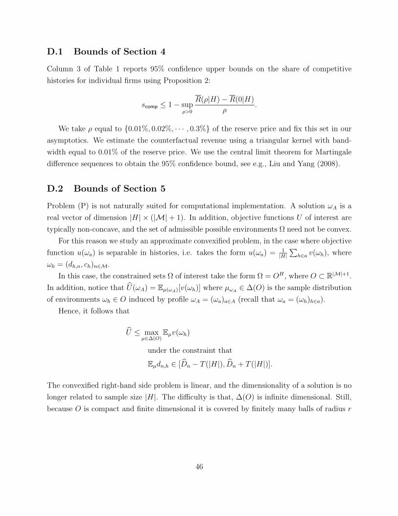
Column 3 of Table 1 reports 95% confidence upper bounds on the share of competitive

histories for individual firms using Proposition 2:

scomp ≤ 1− supρ>0

R(ρ|H)−R(0|H)

ρ.

We take ρ equal to 0.01%, 0.02%, · · · , 0.3% of the reserve price and fix this set in our

asymptotics. We estimate the counterfactual revenue using a triangular kernel with band-

width equal to 0.01% of the reserve price. We use the central limit theorem for Martingale

difference sequences to obtain the 95% confidence bound, see e.g., Liu and Yang (2008).

D.2 Bounds of Section 5

Problem (P) is not naturally suited for computational implementation. A solution ωA is a

real vector of dimension |H| × (|M| + 1). In addition, objective functions U of interest are

typically non-concave, and the set of admissible possible environments Ω need not be convex.

For this reason we study an approximate convexified problem, in the case where objective

function u(ωa) is separable in histories, i.e. takes the form u(ωa) = 1|H|∑

h∈a v(ωh), where

ωh = (dh,n, ch)n∈M.

In this case, the constrained sets Ω of interest take the form Ω = OH , where O ⊂ R|M|+1.

In addition, notice that U(ωA) = Eµ(ωA)[v(ωh)] where µωA∈ ∆(O) is the sample distribution

of environments ωh ∈ O induced by profile ωA = (ωa)a∈A (recall that ωa = (ωh)h∈a).

Hence, it follows that

U ≤ maxµ∈∆(O)

Eµv(ωh)

under the constraint that

Eµdn,h ∈ [Dn − T (|H|), Dn + T (|H|)].

The convexified right-hand side problem is linear, and the dimensionality of a solution is no

longer related to sample size |H|. The difficulty is that, ∆(O) is infinite dimensional. Still,

because O is compact and finite dimensional it is covered by finitely many balls of radius r

46

for any r > 0. Hence for all N , there exists a finite set O′ ⊂ O such that

U − 1

N≤ max

µ∈∆(O′)|H| × Eµv(ωh) (CVX-P)

under the constraint that

Eµdn,h ∈ [Dn − T (|H|), Dn + T (|H|)].

The right-hand-side problem is now a well behaved finite dimensional linear problem. Prac-

tically we use the following algorithm, which starts with an empty seed O∗0 = ∅. At each

stage T ≥ 1 of the algorithm, we perform the following operations:

1. Draw a sample ST of K points in O using a full-support distribution over O.

2. Set OT = O∗T−1 ∪ ST , and solve (CVX-P) for OT ; get solution µT .

3. Set O∗T = suppµT .

4. Iterate until convergence.

E Proofs

E.1 Proofs of Section 3

Proof of Lemma 1. Let H be an adapted set of histories, and fix ρ ∈ (−1,∞). For each

history hi,t = (ht, zi,t) ∈ H, define

εi,t ≡ Eσ[1∧b−i,t>bi,t(1+ρ)|hi,t]− 1∧b−i,t>bi,t(1+ρ)

= probσ(∧b−i,t > bi,t(1 + ρ)|hi,t)− 1∧b−i,t>bi,t(1+ρ).

Note that D(ρ|H)−D(ρ|H) = 1|H|∑

hi,t∈H εi,t.

Note further that, by the law of iterated expectations, for all histories hj,t−s ∈ H with

s ≥ 0, Eσ[εi,t|hj,t−s] = Eσ[Eσ[1∧b−i,t>bi,t(1+ρ)|ht, zi,t]− 1∧b−i,t>bi,t(1+ρ)|ht−s, zj,t−s] = 0.28

Number the histories in H as 1, · · · , |H| such that, for any pair of histories k = (hs, zi,s) ∈H and k′ = (hs′ , zj,s′) ∈ H with k′ > k, s′ ≥ s. For each history k = (ht, zi,t), let εk = εi,t,

28This holds since, in a perfect public Bayesian equilibrium, bidders’ strategies at any time t depend solelyon the public history and on their private information at time t.

47

so that

D(ρ|H)−D(ρ|H) =1

|H|

|H|∑k=1

εk.

Note that, for all k ≤ |H|, Sk ≡∑k

k=1 εk is a Martingale, with increments εk whose

absolute value is bounded above by 1. By the Azuma-Hoeffding Inequality, for every

α > 0, prob(|S|H|| ≥ |H|α) ≤ 2 exp−α2|H|/2. Therefore, with probability 1, 1|H|S|H| =

D(ρ|H)−D(ρ|H) converges to zero as |H| → ∞.


Proof of Proposition 3. By Lemma 1, under the true environment ωA ∈ Ω,

prob(|Dn(H)−Dn(ωA, H)| ≥ T (|H|)

)≤ 2 exp(−T (|H|)2|H|/2)

for each deviation n. It then follows that

prob(∀n, |Dn(H)−Dn(ωA, H)| ≥ T (|H|)

)≤ 2|M| exp(−T (|H|)2|H|/2).

This implies that, with probability at least 1−2|M| exp(−T (|H|)2|H|/2), the constraints in

Program (P) are satisfied when we set the environment equal to ωA. Hence, with probability

at least 1− 2|M| exp(−T (|H|)2|H|/2), U ≥ U(ωA).

Proof of Corollary 2. Suppose the true environment ωA ∈ Ω is such that the indus-

try (or the firms who placed bids in histories H) is competitive. Then Hcomp(ωA) = H,

and so the true share of competitive histories under ωA is scomp = 1 ≥ s0. By Corollary

1, with probability at least 1 − 2|M| exp(−T (|H|)2|H|/2), U ≥ scomp = 1 ≥ s0. Since

2|M| exp(−T (|H|)2|H|/2) → 0 as |H| → ∞, firms in this industry pass test τ with proba-

bility approaching 1 as |H| → ∞.


Proof of Proposition 4. We start by showing that, when penalty K is sufficiently large,

any σ ∈ Σ(K) has the property that all firms pass the test with probability 1, both on and

48

off the path of play. To see why, note first that for every i ∈ N and every strategy profile σ−i

of i’s opponents, firm i can guarantee to pass the test by playing a stage-game best reply to

σ−i at every history. This implies that each firm’s continuation payoff cannot be lower than

0 at any history.

Let K = δ1−δr = δ

1−δ (recall that the reserve price r is normalized to 1), and suppose that

K > K. Towards a contradiction, suppose there exist σ ∈ Σ(K) and a public history ht (on

or off path) such that, at this history, firm i expects to fail the test with strictly positive

probability under σ. Then, for every ε > 0 small, there must exist a public history hs with

s ≥ 0 such that, at the concatenated history ht t hs, firm i expects to fail the test with

probability at least KK

+ ε < 1. Hence, under history ht t hs, firm i’s continuation payoff

at the end of period t + s (i.e., after the outcome of the auction is determined) is bounded

above by δ1−δ −

(KK

+ ε)K = −εK < 0, a contradiction.

For any strategy profile σ and any history hi,t = (ht, zi,t), let Vi(σ, hi,t) = Eσ[∑

s≥t δsui,s|hi,t]

denote firm i’s continuation payoff excluding penalties under σ at history hi,t. Firm i’s total

payoff under strategy profile σ given history hi,t is Vi(σ, hi,t)− Eσ[τi|hi,t]K.

Suppose K > K and fix σ ∈ Σ(K). Since σ is an equilibrium, there cannot be profitable

deviations; in particular, there cannot be profitable one shot deviations:29 for every i ∈ N ,

every history hi,τ , and every one-shot deviation σi 6= σi with σi(hi,t) = σi(hi,t) for all hi,t 6=hi,τ ,

Vi((σi, σ−i), hi,τ )− E(σi,σ−i)[τi|hi,τ ]K ≤ Vi(σ, hi,τ )− Eσ[τi|hi,τ ]K

⇐⇒ Vi((σi, σ−i), hi,τ ) ≤ Vi(σ, hi,τ ), (10)

where the second line in (10) follows since, under equilibrium σ ∈ Σ(K), all firms pass

the test with probability 1 at every history. By the second line in (10), in the game with

K = 0 (i.e., no regulator) no firm has a profitable one shot deviation under strategy profile

σ. Hence, by the one-shot deviation principle σ ∈ Σ(0).30

The following Lemma establishes a weaker version of the one-shot revelation principle for

the game with a regulator.

Lemma E.1. Let σ be a strategy profile with the property that all firms pass the test with

29Note that we are not using the one-shot deviation principle here (which may not hold since the gameis not continuous at infinity when K > 0); we are only using the fact that, in any equilibrium, no player canhave a profitable deviation.

30Note that the game with K = 0 is continuous at infinity, and so the one-shot deviation principle holds.

49

probability 1 at every history. Then, σ ∈ Σ(K) if and only if there are no profitable one-shot

deviations.

Proof. Let σ be a strategy profile with the property that all firms pass the test with prob-

ability 1 at every history. Clearly, if σ ∈ Σ(K), there are no profitable one-shot deviations.

Suppose next that there are no profitable one-shot deviations, but σ /∈ Σ(K). Then, there

exists a player i ∈ N a history hi,t and a strategy σi such that

Vi((σi, σ−i), hi,t) ≥ Vi((σi, σ−i), hi,t)− E(σi,σ−i)[τi|hi,t]K

> Vi(σ, hi,t)− Eσ[τi|hi,τ ]K = Vi(σ, hi,t),

where the last equality follows since σ is such that all firms pass the test with probability 1

at every history.

The proof now proceeds as in the proof of the one-shot deviation principle in games

that are continuous at infinity. Let ε ≡ Vi((σi, σ−i), hi,t) − Vi(σ, hi,t). Let T > 0 be such

that δT

1−δ × r = δT

1−δ < ε/2. Let σi be a strategy for firm i that coincides with σi for all

histories of length t + T or less, and coincides with σi for all histories of length strictly

longer than t + T . Since firms’ flow payoffs are bounded above by r = 1, it must be that

Vi((σi, σ−i), hi,t) − Vi(σ, hi,t) ≥ ε/2. Moreover, since σ is such that all firms pass the test

with probability 1 at all histories, and since σi differs from σi only at finitely many periods,

all firms pass the test under (σi, σ−i) with probability 1 at every history.

Next, look at histories of length t + T . If there exists a history hi,t+T of length t + T

that is consistent with hi,t and such that Vi((σi, σ−i), hi,t+T ) > Vi(σ, hi,t+T ), then there exists

a profitable one shot deviation from σ (since σi and σi coincide for all histories of length

t+ T + 1 or longer).

Otherwise, let σ1i be a strategy that coincides with σi at all histories of length t+T −1 or

less, and that coincides with σi at all histories of length strictly longer than t+ T − 1. Note

that it must be that Vi((σ1i , σ−i), hi,t) − Vi(σ, hi,t) ≥ ε/2. We can now look at histories of

length t+T − 1 that are consistent with hi,t. If there exists such a history hi,t+T−1 such that

Vi((σ1i , σ−i), hi,t+T−1) > Vi(σ, hi,t+T−1), then there exists a profitable one shot deviation from

σ. Otherwise, we can continue in the same way. Since Vi((σi, σ−i), hi,t) − Vi(σ, hi,t) ≥ ε/2,

eventually we will find a profitable one shot deviation by player i, a contradiction.

Proof of Corollary 3. Fix K > K. The proof of Proposition 4 shows that, in all equilibria

in Σ(K), all firms pass the test with probability 1 at every history. Since Σ(K) ⊂ Σ(0), it

50

follows that Σ(K) ⊂ ΣP (0).

We now show that ΣP (0) ⊂ Σ(K). Fix σ ∈ ΣP (0). Since σ is an equilibrium of the game

without a regulator, there cannot be profitable one shot deviations: for every i ∈ N , every

history hi,τ , and every one-shot deviation σi 6= σi with σi(hi,t) = σi(hi,t) for all hi,t 6= hi,τ ,

Vi((σi, σ−i), hi,τ ) ≤ Vi(σ, hi,τ )

⇐⇒ Vi((σi, σ−i), hi,τ )− E(σi,σ−i)[τi|hi,τ ]K ≤ Vi(σ, hi,τ )− Eσ[τi|hi,τ ]K

where the second line follows since, under σ, all firms pass the test with probability 1 at

every history. Lemma E.1 then implies that σ ∈ Σ(K).

Proof of Proposition 5. The proof is similar to the proof of Proposition 4. We first show

that, when penalty K is sufficiently large, any σ ∈ Σ+RP (K) has the property that all firms

pass the test with probability 1, both on and off the path of play.

To show this, we first note that, at any equilibrium in Σ+RP (K) and at every history ht, at

least one firm’s continuation payoff is larger than 0. Indeed, by definition, all firms’ payoffs

at the start of the game are weakly larger than 0 at any equilibrium in Σ+RP (K). By weak

renegotiation proofness, it must be that at every history ht at least one firm’s payoff is larger

than 0.

Recall that K ≡ δ1−δ . Suppose K > K, and fix σ ∈ Σ+

RP (K). Towards a contradiction,

suppose that there exists a history ht (on or off path) such that, at this history, firms expect

to fail the test with strictly positive probability. Then, for every ε > 0 small, there must

exist a history hs with s ≥ 0 such that, at the concatenated history ht t hs, firms expect to

fail the test with probability at least KK

+ ε < 1. Hence, under public history ht t hs, each

firm’s continuation payoff at the end of period t+ s (i.e., after the outcome of the auction is

determined) is bounded above by δ1−δ −

(KK

+ ε)K = −εK < 0, a contradiction.

Suppose K > K and fix σ ∈ Σ+RP (K). Since σ is an equilibrium, there cannot be

profitable deviations; in particular, there cannot be profitable one shot deviations: for every

i ∈ N , every history hi,τ , and every one-shot deviation σi 6= σi with σi(hi,t) = σi(hi,t) for all

hi,t 6= hi,τ ,

Vi((σi, σ−i), hi,τ )− E(σi,σ−i)[τi|hi,τ ]K ≤ Vi(σ, hi,τ )− Eσ[τi|hi,τ ]K

⇐⇒ Vi((σi, σ−i), hi,τ ) ≤ Vi(σ, hi,τ ), (11)

where the second line in (11) follows since, under equilibrium σ, firms pass the test with

51

probability 1 at every history. By the second line in (11), in the game with K = 0 (i.e.,

no regulator) no firm has a profitable one shot deviation under strategy profile σ. By the

one-shot deviation principle, σ ∈ Σ(0). Finally, since σ is weakly renegotiation proof under

penalty K > K, σ must also be weakly renegotiation proof under penalty K = 0. Therefore,

σ ∈ Σ+RP (0).

References

Abdulkadiroglu, A. and K.-S. Chung (2003): “Auction design with tacit collusion,”

Columbia and Northwestern University Working Paper.

Afriat, S. N. (1967): “The construction of utility functions from expenditure data,” In-

ternational economic review, 8, 67–77.

Asker, J. (2010): “A study of the internal organization of a bidding cartel,” The American

Economic Review, 724–762.

Athey, S. and K. Bagwell (2001): “Optimal collusion with private information,” RAND

Journal of Economics, 32, 428–465.

——— (2008): “Collusion with persistent cost shocks,” Econometrica, 76, 493–540.

Bajari, P. and L. Ye (2003): “Deciding between competition and collusion,” Review of

Economics and Statistics, 85, 971–989.

Bergemann, D., B. Brooks, and S. Morris (2017): “First-Price Auctions With Gen-

eral Information Structures: Implications for Bidding and Revenue,” Econometrica, 85,

107–143.

Bergemann, D. and S. Morris (2013): “Robust predictions in games with incomplete

information,” Econometrica, 81, 1251–1308.

——— (2016): “Bayes correlated equilibrium and the comparison of information structures

in games,” Theoretical Economics, 11, 487–522.

Besanko, D. and D. F. Spulber (1989): “Antitrust enforcement under asymmetric

information,” The Economic Journal, 99, 408–425.

52

Carvajal, A., R. Deb, J. Fenske, and J. K.-H. Quah (2013): “Revealed preference

tests of the Cournot model,” Econometrica, 81, 2351–2379.

Chambers, C. P. and F. Echenique (2016): Revealed preference theory, vol. 56, Cam-

bridge University Press.

Chassang, S. and J. Ortner (forthcoming): “Collusion in Auctions with Constrained

Bids: Theory and Evidence from Public Procurement,” Journal of Political Economy.

Che, Y.-K., D. Condorelli, and J. Kim (2018): “Weak cartels and collusion-proof

auctions,” Journal of Economic Theory, 178, 398–435.

Che, Y.-K. and J. Kim (2006): “Robustly Collusion-Proof Implementation,” Economet-

rica, 74, 1063–1107.

Clark, R., D. Coviello, J.-F. Gauthier, and A. Shneyerov (2018): “Bid rigging

and entry deterrence in public procurement: Evidence from an investigation into collusion

and corruption in Quebec,” The Journal of Law, Economics, and Organization, 34, 301–

363.

Clark, R. and J.-F. Houde (2013): “Collusion with asymmetric retailers: Evidence from

a gasoline price-fixing case,” American Economic Journal: Microeconomics, 5, 97–123.

Conley, T. G. and F. Decarolis (2016): “Detecting bidders groups in collusive auc-

tions,” American Economic Journal: Microeconomics, 8, 1–38.

Cyrenne, P. (1999): “On antitrust enforcement and the deterrence of collusive behaviour,”

Review of Industrial Organization, 14, 257–272.

DOJ, U. (2005): “Price fixing, bid rigging, and market allocation schemes: What they are

and what to look for. An Antitrust Primer.” 2005.

Doval, L. and J. Ely (2019): “Sequential information design,” Tech. rep., Working Paper.

Echenique, F., S. Lee, and M. Shum (2011): “The money pump as a measure of revealed

preference violations,” Journal of Political Economy, 119, 1201–1223.

Ellison, G. (1994): “Theories of cartel stability and the joint executive committee,” The

Rand journal of economics, 37–57.

53

Farrell, J. and E. Maskin (1989): “Renegotiation in repeated games,” Games and

economic behavior, 1, 327–360.

Green, E. J. and R. H. Porter (1984): “Noncooperative collusion under imperfect price

information,” Econometrica: Journal of the Econometric Society, 87–100.

Harrington, J. E. (2004): “Cartel pricing dynamics in the presence of an antitrust au-

thority,” RAND Journal of Economics, 651–673.

——— (2008): “Detecting cartels,” Handbook of antitrust economics, 213, 245.

Hart, S. and A. Mas-Colell (2000): “A simple adaptive procedure leading to correlated

equilibrium,” Econometrica, 68, 1127–1150.

Imhof, D., Y. Karagok, and S. Rutz (2016): “Screening for bid-rigging-does it work?”

Tech. rep., Universite de Fribourg.

Kawai, K. and J. Nakabayashi (2018): “Detecting Large-Scale Collusion in Procurement

Auctions,” Available at SSRN 2467175.

LaCasse, C. (1995): “Bid rigging and the threat of government prosecution,” The RAND

Journal of Economics, 398–417.

Levin, J. (2003): “Relational incentive contracts,” The American Economic Review, 93,

835–857.

Liu, R. and L. Yang (2008): “Kernel estimation of multivariate cumulative distribution

function,” Journal of Nonparametric Statistics, 20, 661–677.

Maskin, E. and J. Tirole (2001): “Markov perfect equilibrium: I. Observable actions,”

Journal of Economic Theory, 100, 191–219.

Pesendorfer, M. (2000): “A study of collusion in first-price auctions,” The Review of

Economic Studies, 67, 381–411.

Porter, R. H. (1983): “A study of cartel stability: the Joint Executive Committee, 1880-

1886,” The Bell Journal of Economics, 301–314.

Porter, R. H. and J. D. Zona (1993): “Detection of Bid Rigging in Procurement

Auctions,” Journal of Political Economy, 101, 518–38.

54

——— (1999): “Ohio School Milk Markets: An Analysis of Bidding,” RAND Journal of

Economics, 30, 263–288.

Rotemberg, J. J. and G. Saloner (1986): “A supergame-theoretic model of price wars

during booms,” The American Economic Review, 390–407.

Schurter, K. (2017): “Identification and inference in first-price auctions with collusion,”

Tech. rep., working Paper, University of Chicago.

Toth, B., M. Fazekas, A. Czibik, and I. J. Toth (2014): “Toolkit for detecting

collusive bidding in public procurement,” With examples from Hungary.

Varian, H. R. (1990): “Goodness-of-fit in optimizing models,” Journal of Econometrics,

46, 125–140.

55

data driven regulation: theory and application to missing bids · menica, roger myerson, ariel...

Documents