Data-Driven Ship Digital Twin for Estimating

the Speed Loss caused by the Marine Fouling

Andrea Coraddua,∗, Luca Onetob, Francesco Baldic, Francesca Cipollinib,Mehmet Atlara, Stefano Saviod

aNaval Architecture, Ocean & Marine EngineeringStrathclyde University, Glasgow G1 1XW, UK

bDIBRIS - University of Genova, Via Opera Pia 13, I-16145 Genova, ItalycEcole Polytechnique Federale de Lausanne, EnergyPolis, 1950 Sione

dDITEN - University of Genova, Via Opera Pia 11a, I-16145 Genova, Italy

Abstract

Shipping is responsible for approximately the 90% of world trade leading tosignificant impacts on the environment. As a consequence, a crucial issuefor the maritime industry is to develop technologies able to increase the shipefficiency, by reducing fuel consumption and unnecessary maintenance op-erations. For example, the marine fouling phenomenon has a deep impact,since to prevent or reduce its growth which affects the ship consumption,costly drydockings for cleaning the hull and the propeller are needed andmust be scheduled based on a speed loss estimation. In this work a datadriven Digital Twin of the ship is built, leveraging on the large amount ofinformation collected from the on-board sensors, and is used for estimatingthe speed loss due to marine fouling. A thorough comparison between theproposed method and ISO 19030, which is the de-facto standard for dealingwith this task, is carried out on real-world data coming from two Handymaxchemical/product tankers. Results clearly show the effectiveness of the pro-posal and its better speedloss prediction accuracy with respect to the ISO19030, thus allowing reducing the fuel consumption due to fouling.

∗Corresponding AuthorEmail addresses: andrea.coraddu@strath.ac.uk (Andrea Coraddu),

luca.oneto@unige.it (Luca Oneto), francesco.baldi@epfl.ch (Francesco Baldi),francesca.cipollini@edu.unige.it (Francesca Cipollini),mehmet.atlar@strath.ac.uk (Mehmet Atlar), stefano.savio@unige.it (StefanoSavio)

Preprint submitted to Ocean Engineering January 28, 2019

Keywords: Hull and propeller maintenance, Fouling, Condition BasedMaintenance, ISO 19030, Digital Twin, Data-Driven Models, DeepLearning.

1. Introduction

As awareness of climate change increases, new research results keep con-firming that there is a need of fast, and strong action (IPCC, 2018). Inter-national maritime transport, while representing approximately 90% of globaltrade and the backbone of global economy, contributes to approximately 2.7%of the global anthropogenic carbon dioxide (CO2) emissions (Smith et al.,2014). While this might appear a limited contribution, if current trends arenot changed shipping will become one of the largest shares of global emis-sions (Anderson and Bows, 2012), since as of today, ships are still almostentirely powered by fossil fuels. While alternative fuels have shown to bepromising (Gilbert et al., 2018), there is a need for ship energy systems tobecome more energy efficient (Lutzen et al., 2017). As a result, sustainableshipping is recognised as one of the biggest challenges of the 21st century1,both for its contribution to CO2 emissions and to other pollutants (Schimvan der Loeff et al., 2018).

In recent years, however, the International Maritime Organization (IMO)has officially adopted an initial strategy aiming at reducing GreenhouseGases (GHG) emissions from shipping by 50%, compared to 2008 levels, by2050, and to work towards phasing out them entirely by the end of the cen-tury (MEPC, 2018). As a consequence, developing new technologies able toboth improve the design of the ships and to maintain their efficiency becomesa crucial issue (Deshpande et al., 2013). In this work, much attention wasfocused on the problem of keeping the ship as much efficient as possible byestimating the degradation state of its components, with the consequent per-formance loss and fuel consumption increase (Krozer et al., 2003). Broadlyspeaking, as far as propulsion systems are concerned, there are mainly threemacro-components in a ship that can degrade: the main engine, the hull, andthe propeller (Adland et al., 2018). Apart from the ordinary regular mainte-nance, the main engine degrades very slowly in time and related effects areonly noticeable after years of operations (Calder, 1992). The hull and the

1http://www.ssi2040.org

2

propeller, instead, are subject to marine fouling, that increases the frictionalresistance of the parts moving through the water and, hence, decreases theirefficiency (Adland et al., 2018). The effects of marine fouling can be clearlyobserved after just a few months of operations (Psaraftis and Kontovas, 2014;Demirel et al., 2017a). Marine fouling, or simply biofouling, is defined as theundesirable accumulation of microorganisms, algae, and animals on artificialsurfaces immersed in seawater (Yebra et al., 2004; Lindgren et al., 2016).On the hull, the presence of fouling increases the roughness of the surface,hence increasing frictional resistance (Schultz, 2004; Kempf, 1937). On thepropeller, the presence of fouling increases the roughness of the blade surface,thus requiring more power to maintain the same speed (Atlar et al., 2002;Seo et al., 2016; Owen et al., 2018). Fouling represents the primary cause ofhull (Candries et al., 2003) and propeller (Khor and Xiao, 2011) performancedegradation.

Currently, shipping companies try to mitigate the problem of hull andpropeller fouling by applying anti-fouling paints on the submerged surfacesand by regularly cleaning the hull (Lam and Lai, 2015). Despite their ef-fectiveness, such methods have some drawbacks. In spite of their prime roleand effectiveness in preventing fouling growth, depending on their types, an-tifouling paints can be expensive (e.g. non-biocidal Fouling Release type)and can be harmful to the marine environment (e.g. biocidal Self-Polishingtypes) (Caric et al., 2016). Moreover, the hull and the propeller are cleanedon the occasion of other dry-docking maintenance events, but this practicedoes not ensure an optimal scheduling of the cleaning procedures (Kjaeret al., 2018). Over a typical 4–5 years sailing interval, inadequate hull andpropeller performance is estimated to reduce the efficiency of the entire worldfleet by 9–12% (CSC, 2011). This comes also as a consequence of the diffi-culty of identifying the actual contribution of fouling to the decrease in shipperformance, and shipping companies have called for the establishment ofa transparent and reliable standard for measuring hull and propeller per-formance (CSC, 2011). A reliable and effective planning of these activitiesshould take into account the speed loss caused by the fouling, to find theoptimal balance between efficiency and costs. For this reason an accurateestimation of the speed loss caused by fouling is needed (Schultz, 2007; Atlaret al., 2018).

However, providing a quantitative estimation of the speed loss associatedto the fouling phenomenon is a challenging task (Demirel et al., 2017a,b;Carchen et al., 2017). The latter depends on many factors, such as the speed

3

and the draft of the ship, the sea state, the wind speed and direction, etc.Furthermore the accumulation of marine organisms on the hull is faster whena vessel is frequently in harbour, stationary, or in high-temperature tropicalwaters (Stevens, 1937).

The state-of-the-art approach for estimating the speed loss can be car-ried out by applying the standard ISO 19030 (ISO 19030-2, 2016) proposedby the International Organization for Standardization (ISO). The ISO 19030prescribes methods for measuring changes in hull and propeller performanceand it defines a set of relevant performance indicators for their maintenance,repair, and retrofit activities. Specifically, the ISO 19030 suggests comparingthe measured performances with the ones obtained during sea trials in par-ticular operating points. This comparison provides an indicator of the hulland propeller efficiency. A continuous monitoring of the efficiency provides areliable estimation of the changes in the performances. Despite its simplicityand effectiveness, the ISO 19030 presents some limitations. The procedurerequires filtering out operating points that are outside the prescribed bound-aries, thus limiting the ability of the method to monitor the ship over a wideset of operating conditions (Koboevic et al., 2018). Moreover, some correc-tions are needed to cope with the environmental disturbances (i.e. winds,waves, and currents). Unfortunately, these corrections require the use ofcomplex fluid dynamics models or additional sea trials (ISO 19030-1, 2016;ISO 19030-2, 2016; ISO 19030-3, 2016).

Some attempts have been made to address the ISO 19030 limitations.Logan (2012) uses measurements of the propeller performance as efficiencyindicators; however, this procedure requires the exclusion of many operatingpoints to eliminate the effects of current, ship motions, rudder, and tran-sients, with techniques similar to the ones reported in the ISO 19030 andwith all their inconveniences. Bialystocki and Konovessis (2016) propose anoperational approach for obtaining an accurate fuel consumption and speedcurve, parametrised for the major influence factors, such as ship’s draft anddisplacement, waves forces and directions, hull and propeller roughness. Theproposed approach, similarly to the ISO 19030 procedure, relies on simplifiedcorrections for environmental disturbances, draught, and speed. This appliesalso for the work proposed by Foteinos et al. (2017), whose method is basedon a correction of measured data based on a physical model of the influenceof wind and waves on ship performance.

While models based on the physical knowledge of the problem are well-established (Logan, 2012; ISO 19030-1, 2016), they often fail in predicting

4

the effect of ship-specific and environmental phenomena. On the other hand,Data-Driven Models (DDMs) can easily take into account many phenomenathanks to the use of large amount of data with little, if no physical knowledgeabout the problem. DDMs have shown to be an effective tool for the solutionof many problems in the shipping industry: condition based maintenance ofthe propulsion system (Cipollini et al., 2018), crash stop maneuvering per-formance prediction (Oneto et al., 2017a), operational profile prediction andoptimisation (Coraddu et al., 2016), fuel consumption prediction and opti-misation (Parlak et al., 2006). In particular, Neural Networks and GaussianProcess were employed to estimate the ship’s fuel consumption efficiencyin Pedersen and Larsen (2009) and Petersen et al. (2012), while in Radonjicand Vukadinovic (2015) a Neural Network Ensemble is exploited for tow-boat shaft power prediction. In Jonge (2017) many different supervised andunsupervised data-analytic models were adopted in order to investigate therelation between several vessel performance and environmental variables. Fi-nally, in Leifsson et al. (2008) the performances of white, grey, and black boxmodels for predicting the fuel consumption are tested.

Deep Learning techniques represent the state-of-the-art for dealing withdata driven problems, despite its limitations. In particular, all the hid-den parameters in Deep Learning framework need to be fine-tuned multipletimes and are affected by the problem of local minima and slow convergencerate (Kasun et al., 2013). Recently some attempts have been made to over-come these limitations.

In particular, ELM (Cambria and Huang, 2013; Huang et al., 2015, 2006a)were introduced to overcome problems posed by back-propagation trainingalgorithm (Huang, 2014, 2015; Ridella et al., 1997; Rumelhart et al., 1988):potentially slow convergence rates, critical tuning of optimisation parame-ters, and presence of local minima that call for multi-start and re-trainingstrategies. The original ELM are also called Shallow ELM (SELM) becausethey have been developed for the single-hidden-layer feedforward neural net-works (Huang et al., 2008, 2006b, 2004), and they have been generalised inorder to cope with cases where ELM are not neuron alike. SELM were laterimproved to cope with problems intractable by shallow architectures (Ben-gio et al., 2013; Vincent et al., 2008; Zhou et al., 2015), by proposing variousDeep ELM (DELM) built upon a deep architecture (Tissera and McDonnell,2016; Oneto et al., 2017b), in order to make possible to extract features by amultilayer feature representation framework. In this work, the use of DELMis proposed for estimating the speed loss caused by the marine fouling effects

5

on the ship hull and propeller, leveraging on the large amount of informationcollected from the on-board monitoring system sensors. Inspired by the ISO19030 and supported by the evidence that DDMs can be much more accurateand effective than the physical ones, a DDM is proposed for predicting thespeed of the ship, able to act as a “Digital Twin” (Glaessgen and Stargel,2012) of the ship itself. The Digital Twin can be used to compute the de-viation between the predicted performance and the actual one, namely thespeed loss (Boschert and Rosen, 2016). It will be shown that the averagedrift in time of the speed loss can be exploited to accurately and effectivelyestimate the effects of the marine fouling on the ship performance, and thusprogram a more efficient hull and propeller cleaning scheduling. To this aim,they propose a two-phase approach:

(I) firstly, a DDM based Digital Twin is built, leveraging on the largeamount of information collected from the on-board monitoring systemsensors;

(II) secondly, the same model is applied in order to estimate the speed-lossof the ship and its drift.

Obviously the Digital Twin needs to be tuned on data collected during aperiod of time where the marine fouling is not present and for a time periodwide enough to observe the ship in many operational and environmentalconditions: data collection can start just after the launch of the ship (or afterhull and propeller cleaning) and stop after some months of operations. DeepLearning techniques represent the state-of-the-art for dealing with Phase (I).For what concerns Phase (II), instead, it will be shown that the averagebehaviour of the speed loss between two maintenance events (where alsohull and propeller cleaning is performed) is characterised by a clear drift,easily detectable with a robust regression (Zhao and Sun, 2010) in time ofthe predicted speed losses. Moreover, it will be shown, by means of thenonparametric statistical test of Kolmogorov-Smirnov (Smirnov, 1944), thatthe distribution of the speed loss before and after two maintenance eventschanges in a statistical significant way while, during the operations, such adistribution changes smoothly.

A comparison between the proposed method and the ISO 19030 on real-world data coming from two Handymax chemical/product tankers has beencarried out and is presented in this work to show the effectiveness of theproposal.

The paper is organised as follows. Section 2 reports a general description

6

of the two Handymax chemical/product tankers, and the monitoring systemdata considered. Section 3 presents a description of the standard applicationof ISO 19030. The proposed approach is described in Section 4. A comparisonbetween the proposed method and the ISO 19030 on real-world data comingfrom the two vessels described in Section 2 is reported in Section 5. Finally,in Section 6, the conclusions of the paper are drawn.

For the benefit of the reader Table 1 containing all the adopted notationwas added.

2. Available Vessels and Data

This section presents the two Handymax chemical/product tankers ex-ploited, their data logging systems, and the available data adopted in thepaper for comparing the proposed method and the ISO 19030, as far as theestimate of the speed loss caused by the marine fouling is concerned.

In this paper operational data available from two Handymax chemi-cal/product tankers are used. The first vessel (V1) was designed and builtfor transporting chemicals and petroleum products up to 46764DWT with adesign speed of 15knots. The vessel is 176.75m long (between perpendicular)and 32.18m wide, run by two four-stroke engines providing a total propulsivepower of 7680kW . The second vessel (V2) is a tanker for chemicals and oilproducts up to 46067DWT with a design speed of 15.5knots. The vessel is176.83m long (between perpendicular) and 32.20m wide, run by a two-strokeengine power of 8200kW . A conceptual representation of the propulsion sys-tem of the two vessels is shown in Figure 1, while their main features arepresented in Table 2.

The first vessel (V1) is equipped with two main engines (MaK 8M32Cfour-stroke Diesel engines rated 3840kW ) and designed for operation at600rpm. The engines are connected to a gearbox that distributes the powerbetween the controllable pitch propeller for propulsion and a shaft generator(rated 3200kW ). Auxiliary power can also be generated by two auxiliaryengines rated 682kW each. Each main engine is equipped with exhaust gasboiler, that can be integrated with two auxiliary oil-fired boilers.

The second vessel (V2) is equipped with one main engine (MAN B&W6S50MC slow speed, two-stroke engine rated 8200kW ) and designed for op-eration at 120rpm. In this case, the auxiliary power is generated by threeDiesel-generators rated 1176kW each. As for V1, the main engine is equipped

7

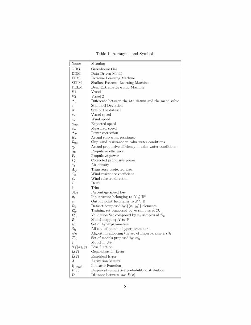
Table 1: Acronyms and Symbols

Name Meaning

GHG Greenhouse GasDDM Data-Driven ModelELM Extreme Learning MachineSELM Shallow Extreme Learning MachineDELM Deep Extreme Learning MachineV1 Vessel 1V2 Vessel 2∆i Difference between the i-th datum and the mean valueσ Standard DeviationN Size of the datasetvv Vessel speedvw Wind speedvexp Expected speedvm Measured speed∆P Power correctionRw Actual ship wind resistanceR0w Ship wind resistance in calm water conditionsηp Actual propulsive efficiency in calm water conditionsη0p Propulsive efficiencyPp Propulsive powerP ′p Corrected propulsive power

ρa Air densityAtp Transverse projected areaCw Wind resistance coefficientψw Wind relative directionT Draftδ TrimSL% Percentage speed lossxi Input vector belonging to X ⊆ Rd

yi Output point belonging to Y ⊆ RDn Dataset composed by {(xi, yi)} elementsLrnl

Training set composed by nl samples of Dn

VrnvValidation Set composed by nv samples of Dn

S Model mapping X to YH Set of hyperparametersSH All sets of possible hyperparametersAH Algorithm adopting the set of hyperparameters HFH Set of models proposed by AHf Model in FH`(f(x), y) Loss functionL(f) Generalization Error

L(f) Empirical ErrorA Activation MatrixI[−∞,x] Indicator Function

F (x) Empirical cumulative probability distributionD Distance between two F (x)

8

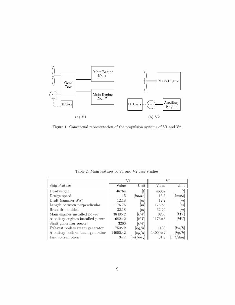
(a) V1 (b) V2

Figure 1: Conceptual representation of the propulsion systems of V1 and V2.

Table 2: Main features of V1 and V2 case studies.

V1 V2Ship Feature Value Unit Value Unit

Deadweight 46764 [t] 46067 [t]Design speed 15 [knots] 15.5 [knots]Draft (summer SW) 12.18 [m] 12.2 [m]Length between perpendicular 176.75 [m] 176.83 [m]Breadth moulded 32.18 [m] 32.20 [m]Main engines installed power 3840×2 [kW ] 8200 [kW ]Auxiliary engines installed power 682×2 [kW ] 1176×3 [kW ]Shaft generator power 3200 [kW ]Exhaust boilers steam generator 750×2 [kg/h] 1130 [kg/h]Auxiliary boilers steam generator 14000×2 [kg/h] 14000×2 [kg/h]Fuel consumption 34.7 [mt/day] 31.8 [mt/day]

9

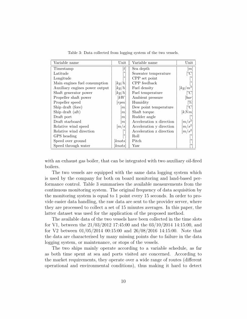
Table 3: Data collected from logging system of the two vessels.

Variable name Unit Variable name Unit

Timestamp [t] Sea depth [m]Latitude [°] Seawater temperature [°C]Longitude [°] CPP set point [°]Main engines fuel consumption [kg/h] CPP feedback [°]Auxiliary engines power output [kg/h] Fuel density [kg/m3]Shaft generator power [kg/h] Fuel temperature [°C]Propeller shaft power [kW ] Ambient pressure [bar]Propeller speed [rpm] Humidity [%]Ship draft (fore) [m] Dew point temperature [°C]Ship draft (aft) [m] Shaft torque [kNm]Draft port [m] Rudder angle [°]Draft starboard [m] Acceleration x direction [m/s2]Relative wind speed [m/s] Acceleration y direction [m/s2]Relative wind direction [°] Acceleration z direction [m/s2]GPS heading [°] Roll [°]Speed over ground [knots] Pitch [°]Speed through water [knots] Yaw [°]

with an exhaust gas boiler, that can be integrated with two auxiliary oil-firedboilers.

The two vessels are equipped with the same data logging system whichis used by the company for both on board monitoring and land-based per-formance control. Table 3 summarises the available measurements from thecontinuous monitoring system. The original frequency of data acquisition bythe monitoring system is equal to 1 point every 15 seconds. In order to pro-vide easier data handling, the raw data are sent to the provider server, wherethey are processed to collect a set of 15 minutes averages. In this paper, thelatter dataset was used for the application of the proposed method.

The available data of the two vessels have been collected in the time slotsfor V1, between the 21/03/2012 17:45:00 and the 03/10/2014 14:15:00, andfor V2 between 01/05/2014 00:15:00 and 26/08/2016 14:15:00. Note thatthe data are characterised by many missing points due to failure in the datalogging system, or maintenance, or stops of the vessels.

The two ships mainly operate according to a variable schedule, as faras both time spent at sea and ports visited are concerned. According tothe market requirements, they operate over a wide range of routes (differentoperational and environmental conditions), thus making it hard to detect

10

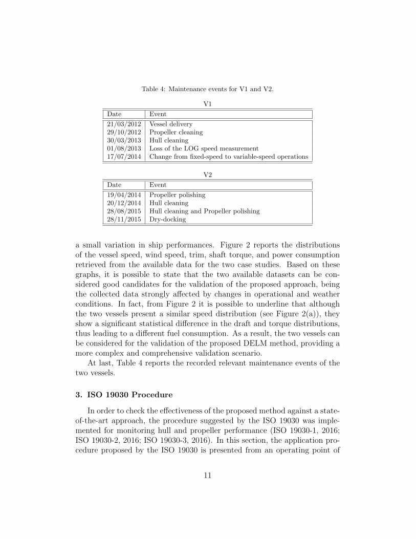
Table 4: Maintenance events for V1 and V2.

V1

Date Event

21/03/2012 Vessel delivery29/10/2012 Propeller cleaning30/03/2013 Hull cleaning01/08/2013 Loss of the LOG speed measurement17/07/2014 Change from fixed-speed to variable-speed operations

V2

Date Event

19/04/2014 Propeller polishing20/12/2014 Hull cleaning28/08/2015 Hull cleaning and Propeller polishing28/11/2015 Dry-docking

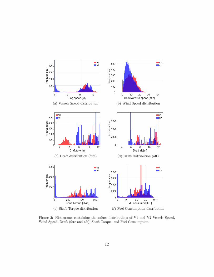
a small variation in ship performances. Figure 2 reports the distributionsof the vessel speed, wind speed, trim, shaft torque, and power consumptionretrieved from the available data for the two case studies. Based on thesegraphs, it is possible to state that the two available datasets can be con-sidered good candidates for the validation of the proposed approach, beingthe collected data strongly affected by changes in operational and weatherconditions. In fact, from Figure 2 it is possible to underline that althoughthe two vessels present a similar speed distribution (see Figure 2(a)), theyshow a significant statistical difference in the draft and torque distributions,thus leading to a different fuel consumption. As a result, the two vessels canbe considered for the validation of the proposed DELM method, providing amore complex and comprehensive validation scenario.

At last, Table 4 reports the recorded relevant maintenance events of thetwo vessels.

3. ISO 19030 Procedure

In order to check the effectiveness of the proposed method against a state-of-the-art approach, the procedure suggested by the ISO 19030 was imple-mented for monitoring hull and propeller performance (ISO 19030-1, 2016;ISO 19030-2, 2016; ISO 19030-3, 2016). In this section, the application pro-cedure proposed by the ISO 19030 is presented from an operating point of

11

(a) Vessels Speed distribution (b) Wind Speed distribution

(c) Draft distribution (fore) (d) Draft distribution (aft)

(e) Shaft Torque distribution (f) Fuel Consumption distribution

Figure 2: Histograms containing the values distributions of V1 and V2 Vessels Speed,Wind Speed, Draft (fore and aft), Shaft Torque, and Fuel Consumption.

12

view. More details are available in the reference documents (ISO 15016:2015,2015). The application of the ISO 19030 procedure, given the informationcollected from the data logging system as reported in Table 3, can be sum-marized in the following steps:

(I) Data filtering(II) Correction for environmental factors

(III) Calculation of Performance Values (PVs)(IV) Calculation of Performance Indicators (PIs)

Step (I) is performed by applying the Chauvenet’s criterion (Chauvenet,1863) to all measured variables, according to which a datum is to be consid-ered an outlier if:

erfc

(∆i

σ√

2

)N < 0.5 (1)

where erfc is the complementary error function (Glaisher, 1871), ∆i repre-sents the difference between the i-th datum and the mean value over thedataset, σ is the standard deviation of the variable of interest, and N thesize of the dataset. In addition, further filtering was applied consideringoutliers also points for which:

vv < 8[knots], |vw| > 8[m/s] (2)

where vv and vw are the speed of vessel and wind respectively. The additionalfiltering on the ship speed was added in order to avoid numerical errors inthe evaluation of the speed loss for low values in the denominator of Eq. (6),while the filter on the wind speed was added to filter out points with badweather conditions, since the behaviour of the vessel in those conditions isstrongly inconstant and unreliable. Step (II) included the power correction∆P based on measurements of wind speed and direction:

∆P = (Rw −R0w)v2v1

η0p+ Pp(1−

ηpηop

) (3)

where Rw represents the ship’s wind resistance due to relative wind, R0w

is the air resistance in no-wind conditions, Pp is the propulsive power, ηp itspropulsive efficiency, and η0p is the propulsive efficiency in calm condition.In absence of more accurate information, ηp is set to 0.7, as suggested by theISO. The ship wind resistance Rrw is computed as follows:

Rrw = 0.5ρav2wAtpCw(ψw) (4)

13

where ρa is the air density, Atp is the transverse projected area, Cw is the windresistance coefficient, and ψw is the wind relative direction. Eq. (4) is usedfor calculating both the actual and the reference wind resistance using therelative wind speed and the relative wind direction in the first case and theship speed and head wind direction in the second case. The wind resistancecoefficient is computed based on Fujiwara et al. (2006).

Step (III) involves the calculation of the percentage speed loss based onthe corrected propulsion power. The expected speed vexp is computed basedon reference, clean-hull data interpolated starting from actual measurementsof draft (T ) and trim (δ):

vexp = f(P ′p, T, δ) (5)

where P ′p is the corrected power for accounting the effect of the draft andtrim. This allows to compute the percentage speed loss SL% as:

SL% = 100vm − vexpvexp

(6)

where vm is the measured speed.The speed loss is then used as performance value for the calculation of

the different performance indicator in Step (IV). The ISO procedure suggestscomparing the average value of the speed loss over a given period of time inorder to average out uncertainties and statistically not-relevant fluctuations.

4. Proposed Approach

In this section the approach proposed in this paper is reported. As dis-cussed in the introduction, the proposal is a two-phases approach:

(I) first a Digital Twin, based on a DDM, is built using a DELM and thedata described in Section 2. The model exploits data collected duringa suitable period of time when the marine fouling is not present and fora period long enough to observe the ship in different operational andenvironmental conditions (e.g. one can start the data collection justafter the launch of the ship or its hull and propeller cleaning and stopafter one or two months of operations);

(II) then the DDM is applied on a second set of data and the speed lossis computed. Subsequently, the drift in the average behaviour of thespeed loss between two maintenance operations is studied, together

14

with changes in its distribution using robust regression and statisticalnonparametric test.

In the next section the two phases will be detailed.

4.1. Phase (I)

Phase (I) consists in mapping the task of predicting the speed of thevessel in a standard regression problem. In this framework (Vapnik, 1998), aset of data Dn = {(x1, y1) , · · · , (xn, yn)}, where xi ∈ X ⊆ Rd are the inputsand yi ∈ Y ⊆ R is an output, needs to be available. The goal is to identifythe unknown model which maps inputs to outputs S : X → Y through analgorithm AH which chooses a model f : X → Y in a set of models FH,defined by some hyperparameters H.

In this specific case, the inputs and the outputs based on the availablemeasurements reported in Table 3 are identified. In particular, Table 5 re-ports the chosen subset of features of the monitoring system adopted as inputand output features for the proposed model. It is worth noting that the se-lected features provide the model with a good representation of the vessel’spropulsion system, its motion and the weather conditions (Coraddu et al.,2015; Petersen et al., 2012). With respect to Table 3, Table 5 discards allthose features which are duplicated, not necessary, or trivially related to thespeed prediction.

The accuracy of f in representing the unknown system S is measuredwith a prescribed loss function ` : Y × Y → [0,∞). Since the consideredproblem is a regression one, the most suited loss function is the squared one`(f(x), y) = [f(x)−y]2 (Rosasco et al., 2004). Then the generalization errorof f , namely the true error of f , can be defined as

L(f) = E(x,y)`(f(x, y)). (7)

Obviously L(f) cannot be computed but its empirical estimator, the empir-ical error, can be derived

L(f) =1

n

n∑i=1

`(f(xi, yi)). (8)

As far as the algorithm AH is concerned, in this paper the DELM isexploited, as described in Section 1. DELM are the evolution of the SELMfor the purpose of creating an algorithm able to both learn new features from

15

Table 5: Input and Output of the Digital Twin for Speed Prediction.

INPUT VARIABLES OUTPUT VARIABLE

Latitude

Speed through water

LongitudeMain engines fuel consumptionAuxiliary engines power outputShaft generator powerPropeller shaft powerPropeller speedShip draft (fore)Ship draft (aft)Draft portDraft starboardSea depthRelative wind speedRelative wind directionGPS headingSea water temperatureCPP set pointCPP feedbackFuel densityFuel temperatureAmbient pressureHumidityDew point temperatureShaft torqueRudder angleAcceleration x directionAcceleration y directionAcceleration z directionRollPitchYaw

16

the available raw variables and create a regression model. For this reason,in order to understand the DELM, first the definition of SELM has to berecalled.

SELM were originally developed for the single-hidden-layer feedforwardneural networks

f(x) =h∑

i=1

wigi(x). (9)

where gi : Rd → R, i ∈ {1, · · · , h} is the hidden-layer output correspondingto the input sample x ∈ Rd, and w ∈ Rh is the output weight vector betweenthe hidden layer and the output layer. In this case, the input layer has dneurons and connects to the hidden layer (having h neurons) through a setof weights W ∈ Rh×(0,··· ,d) and a nonlinear activation function2, ϕ : R → R.Thus, the i-th hidden neuron response to an input stimulus x is:

gi(x) = ϕ

(Wi,0 +

d∑j=1

Wi,jxj

). (10)

In SELM, the parameters W are set randomly. A vector of weighted links,w ∈ Rh, connects the hidden neurons to the output neuron without any bias.The overall output function of the network (see Figure 3) is:

f(x)=h∑

i=1

wiϕ

(Wi,0+

d∑j=1

Wi,jxj

)=

h∑i=1

wiϕi(x). (11)

It is convenient to define an activation matrix, A ∈ Rn×h, such that theentry Ai,j is the activation value of the j-th hidden neuron for the i-th inputpattern. The A matrix is:

A =

[ϕ1(x1) ··· ϕh(x1)

......

...ϕ1(xn) ··· ϕh(xn)

]. (12)

In the SELM model the weights W are set randomly and are not subject toany adjustment, and the quantity w in Eq. (11) is the only degree of freedom.

2In this work the tanh function was adopted as suggested in the original work of Huanget al. (2004), nevertheless using other activation functions such as the sigmoidal one doesnot really affect the final performance.

17

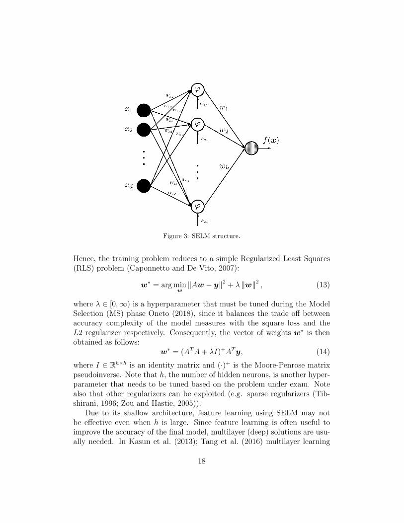
Figure 3: SELM structure.

Hence, the training problem reduces to a simple Regularized Least Squares(RLS) problem (Caponnetto and De Vito, 2007):

w∗ = arg minw‖Aw − y‖2 + λ ‖w‖2 , (13)

where λ ∈ [0,∞) is a hyperparameter that must be tuned during the ModelSelection (MS) phase Oneto (2018), since it balances the trade off betweenaccuracy complexity of the model measures with the square loss and theL2 regularizer respectively. Consequently, the vector of weights w∗ is thenobtained as follows:

w∗ = (ATA+ λI)+ATy, (14)

where I ∈ Rh×h is an identity matrix and (·)+ is the Moore-Penrose matrixpseudoinverse. Note that h, the number of hidden neurons, is another hyper-parameter that needs to be tuned based on the problem under exam. Notealso that other regularizers can be exploited (e.g. sparse regularizers (Tib-shirani, 1996; Zou and Hastie, 2005)).

Due to its shallow architecture, feature learning using SELM may notbe effective even when h is large. Since feature learning is often useful toimprove the accuracy of the final model, multilayer (deep) solutions are usu-ally needed. In Kasun et al. (2013); Tang et al. (2016) multilayer learning

18

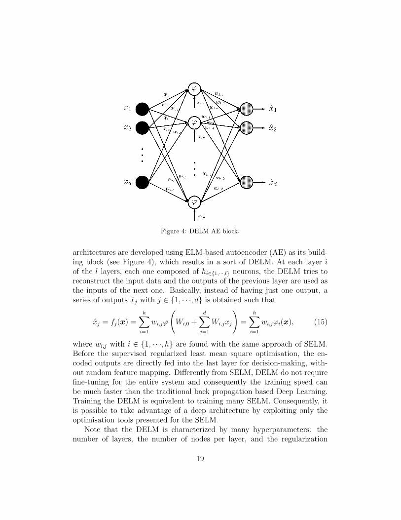
Figure 4: DELM AE block.

architectures are developed using ELM-based autoencoder (AE) as its build-ing block (see Figure 4), which results in a sort of DELM. At each layer iof the l layers, each one composed of hi∈{1,···,l} neurons, the DELM tries toreconstruct the input data and the outputs of the previous layer are used asthe inputs of the next one. Basically, instead of having just one output, aseries of outputs xj with j ∈ {1, · · ·, d} is obtained such that

xj = fj(x) =h∑

i=1

wi,jϕ

(Wi,0 +

d∑j=1

Wi,jxj

)=

h∑i=1

wi,jϕi(x), (15)

where wi,j with i ∈ {1, · · ·, h} are found with the same approach of SELM.Before the supervised regularized least mean square optimisation, the en-coded outputs are directly fed into the last layer for decision-making, with-out random feature mapping. Differently from SELM, DELM do not requirefine-tuning for the entire system and consequently the training speed canbe much faster than the traditional back propagation based Deep Learning.Training the DELM is equivalent to training many SELM. Consequently, itis possible to take advantage of a deep architecture by exploiting only theoptimisation tools presented for the SELM.

Note that the DELM is characterized by many hyperparameters: thenumber of layers, the number of nodes per layer, and the regularization

19

coefficient: H = {l, h1, · · · , hl, λ}. H must be carefully tuned in order toobtain the smallest generalization error of the final model. For this pur-pose a MS phase needs to be performed (Oneto, 2018). In this work thenonparametric Bootstrap (BTS) approach is employed as it is a frequentlyadopted state-of-the-art MS method in the family of the resampling meth-ods. Resampling methods derive their name from the procedure of resam-pling once or many (nr) times, with or without replacement, the originaldataset Dn, in order to build two independent datasets called training, andvalidation sets, respectively Lr

nland Vr

nv, with r ∈ {1, · · · , nr}. Note that

Lrnl∩Vr

nv= �, Lr

nl∪Vr

nv= Dn. Then, in order to perform the MS phase and

select the best combination of the hyperparameters H in a set of possibleones SH = {H1,H2, · · · } for the algorithm AH, the following procedure hasto be applied:

H∗ : minH∈SH

1

nr

nr∑r=1

1

nv

∑(x,y)∈Vr

nv

`(AH,Lrnl(x), y), (16)

where AH,Lrnlis a model built with the algorithm AH trained with Lr

nl. Since

the data in Lrnl

are independent with respect to the ones in Vrnv

, H∗ shouldachieve low error rates on a data set which is different from the one usedfor training purposes. BTS differentiates from the other resampling methodssince nl = n and since Lr

nlis sampled with replacement from Dn. Note that

Vrnv

= Dn \ Lrnl

.

4.2. Phase (II)

Once the DELM based Digital Twin has been built, it is possible to applyit to the rest of the data in order to estimate the expected speed vexpected andcompare it with the measured one vmeasured for the purpose of computing thepercentage speed loss SL%. Note that this can be done both in a data drivenway (see Section 4.1) and with the ISO 19030 (see Section 3).

The result of this process is a series of values in time representing thetrend of the percentage speed loss

SL%(t), t ∈ {t1, t2, · · · }, t1 < t2 < · · · . (17)

The time series obtained with the DELM are referred as SLDELM% (t), while

SLISO% (t) are the one obtained with the ISO 19030.The mentioned time series can be studied in two ways.

20

In the first case the drift in the behaviour of the SL%(t) between twopropeller and/or hull cleaning events was studied, by finding the best linearregressor for the speed loss percentage. Note that the time series computedfrom the data, as also observed by the ISO 19030, is characterized by un-certainties and irrelevant statistically fluctuations. For this reason, insteadof applying a simple RLS, the robust regression developed in Zhao and Sun(2010) has been used. The idea of the robust regression applied to this caseis quite simple. Firstly the regressor function had to be defined, in this casea linear regressor in time g(t) = at + b with a, b ∈ R. Then instead ofminimizing the mean square error, the following costs have been minimized

a∗, b∗ = arg mina,b∈R

∑t∈{t1,t2,··· }

max[min[at+ b− SL%(t), ε], ε] (18)

where ε and ε are hyperparameters that needs to be tuned. Note that, ba-sically, robust regression exploits a loss function which does not take intoaccount too small or too large errors. Unfortunately, this loss is nonconvexand in Zhao and Sun (2010) a method for facing this issue is proposed. Therobust regression allows obtaining results which are not affected by the highnumber of outliers observed in the time series (see Section 5).

In the second case, the automatic identification of changes in time of thedistribution of the percentage speed loss was tried, in order to check if thosechanges were in correspondence to maintenance activities, and testify thequality of the estimated speed loss. For this purpose Kolmogorov–Smirnovtest (Smirnov, 1944) has been adopted. This nonparametric statistical testcan be exploited to check if two different data samples of data are derivedfrom the same probability distribution. The Null Hypothesis is that the twosamples belong to the same distribution. Then the test tries to quantifythe distance between the distributions of the two samples and, if the dis-tance is greater than a specific threshold, the hypothesis is rejected. Thedistance between the two samples SA = {SL%(t − ∆), · · · , SL%(t)} andSB = {SL%(t), · · · , SL%(t + ∆)}, is computed exploiting the empirical cu-mulative probability distribution F j(x) of the two different samples, withj ∈ A,B which is defined as:

Fj(x) =1

n

n∑i=1

ISji≤x

(19)

where I[−∞,x](Sji ) is the indicator function, equal to 1 if Sj

i ≤ x and equal to 0otherwise. The distance D between FA(x) and FB(x) is computed adopting

21

the following metric:

D = sup−∞<x<+∞

∣∣FA(x)− FB(x)∣∣ (20)

For the analysis carried out in this paper, the maximum D value tolerableto refuse the hypotheses was set at 95%. The test was applied by comparingsubsequent non-overlapping time windows of 30 days, in order to detect abroad variation in the series. It is worth noting that if the test is rejected,then a major change in the distribution of the error has occurred, thus indi-cating that the state of the vessel has abruptly changed.

5. Results and discussion

In this section, the available data described in Section 2 are exploitedfor the purpose of making a detailed comparison between the results ob-tained through the state-of-art ISO 19030 procedure, and the ones achievedvia the DELM model. In particular, the properties of the speed losses es-timated with the two models for both V1 and V2 are compared. The ISO19030 model is built exploiting the procedure described in Section 3, whilethe DELM model is built adopting data for two months of historical data,in the proximity of a ship hull and propeller cleaning (for V1 the time slotbetween the 01/07/2012 and the 15/09/2012, and for V2 the one betweenthe 15/01/2016 and the 15/06/2016), using the procedure described in Sec-tion 4.1. Moreover, as far as the MS phase is concerned, the best set ofhyperparameters was searched in

SH={{1, 2, 4, 8, 16, 32}×10{1,2,3,4}×· · ·×10{1,2,3,4}×{10−6, 10−5.5, · · ·, 104}}.

As results will show, despite the accuracy and reliability of the sensorsmeasurements collected on-board cannot be ensured (Coraddu et al., 2017),the proposed DELM allows the identification of clear drift in the performanceof the vessel compared to the ISO 19030 procedure.

5.1. Distributions of DELM and ISO 19030 Estimated Percentage Speed Loss

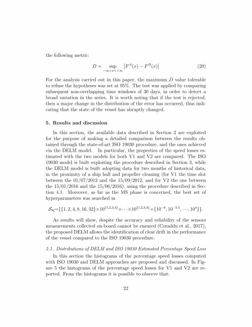
In this section the histograms of the percentage speed losses computedwith ISO 19030 and DELM approaches are proposed and discussed. In Fig-ure 5 the histograms of the percentage speed losses for V1 and V2 are re-ported. From the histograms it is possible to observe that:

22

(a) V1 (b) V2

Figure 5: Histograms of DELM and ISO 19030 Estimated Percentage Speed Loss.

• as expected, the variance of the distribution of the percentage speedlosses is lager for the DELM model with respect to the one of the ISO19030. This is caused by the fact that the ISO 19030 filters out a largeamount of data points, only keeping those for which the application ofthe method is more reliable (see Section 3). On the other hand, theDELM model exploits all the available data points corresponding to alarger variety of operational conditions;

• the average of the distribution of the speed loss is not always centeredon a positive value, due to the fact that the data used for training theDELM and the parameters used for the ISO 19030 do not correspondto a perfect clean state, as it would be required for creating a perfectdigital twin (as shown later, this problem does not affect the quality ofthe final results);

• the results obtained by the two models are, at least qualitatively, inan overall good agreement (quantitative assessment will be discussedin the next section).

5.2. Scatterplot of DELM and ISO 19030 Estimated Percentage Speed Loss

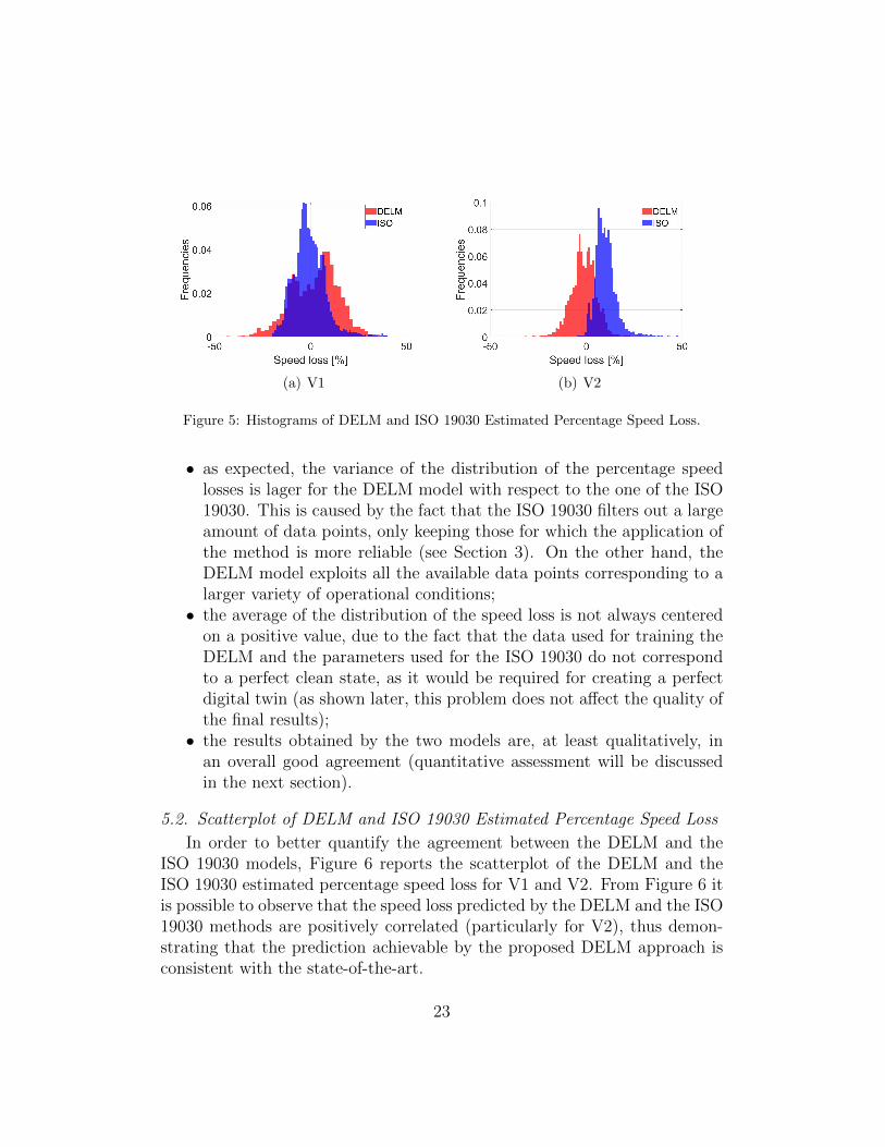
In order to better quantify the agreement between the DELM and theISO 19030 models, Figure 6 reports the scatterplot of the DELM and theISO 19030 estimated percentage speed loss for V1 and V2. From Figure 6 itis possible to observe that the speed loss predicted by the DELM and the ISO19030 methods are positively correlated (particularly for V2), thus demon-strating that the prediction achievable by the proposed DELM approach isconsistent with the state-of-the-art.

23

(a) V1 (b) V2

Figure 6: Scatterplot of the DELM and the ISO 19030 Estimated Speed Loss Percentages.

5.3. Drift in DELM and ISO 19030 Estimated Percentage Speed Loss

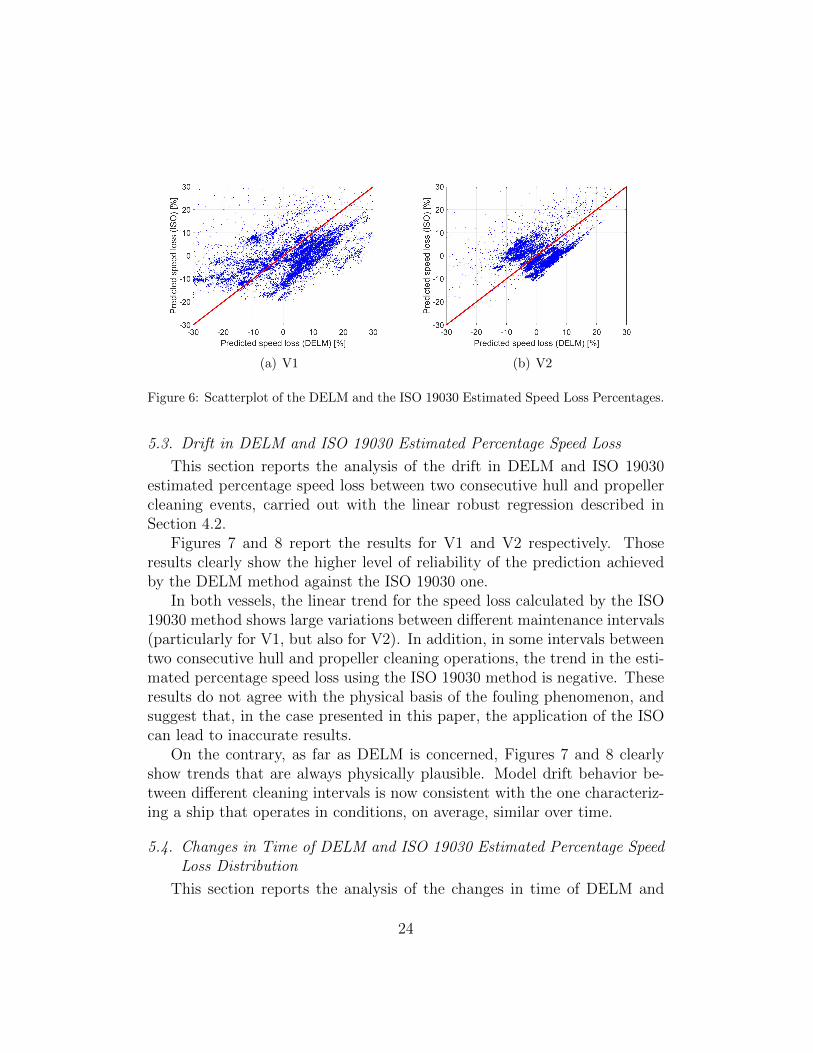
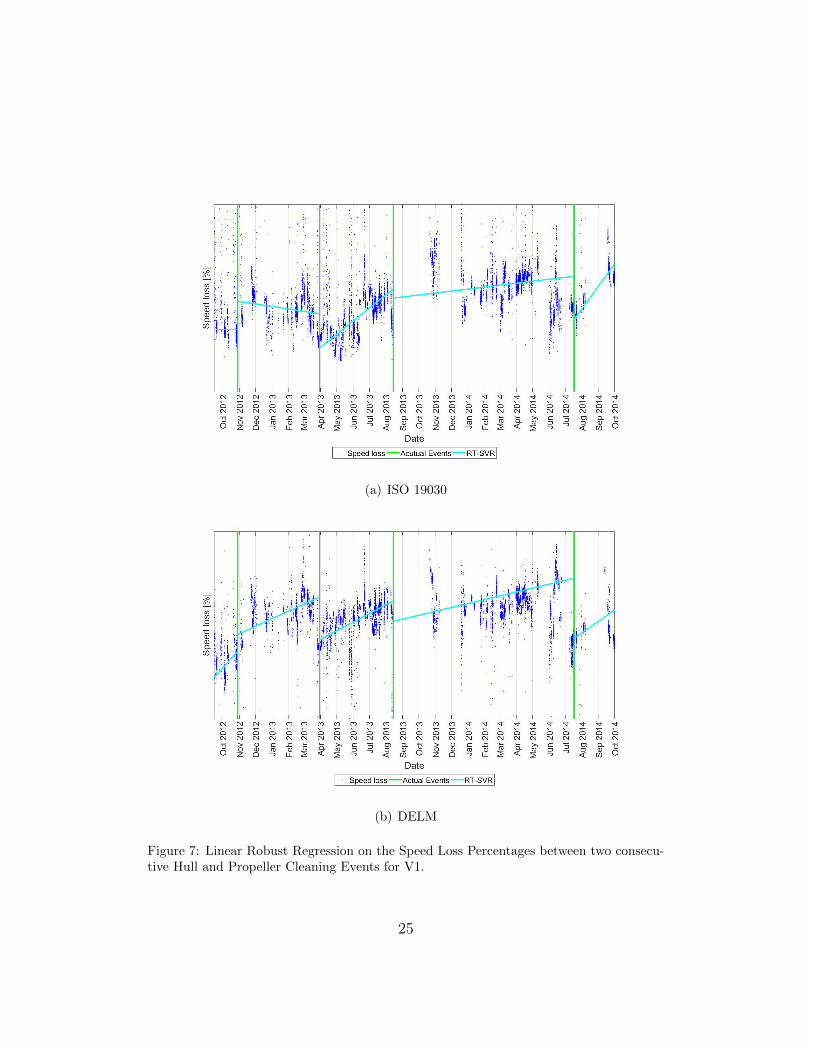
This section reports the analysis of the drift in DELM and ISO 19030estimated percentage speed loss between two consecutive hull and propellercleaning events, carried out with the linear robust regression described inSection 4.2.

Figures 7 and 8 report the results for V1 and V2 respectively. Thoseresults clearly show the higher level of reliability of the prediction achievedby the DELM method against the ISO 19030 one.

In both vessels, the linear trend for the speed loss calculated by the ISO19030 method shows large variations between different maintenance intervals(particularly for V1, but also for V2). In addition, in some intervals betweentwo consecutive hull and propeller cleaning operations, the trend in the esti-mated percentage speed loss using the ISO 19030 method is negative. Theseresults do not agree with the physical basis of the fouling phenomenon, andsuggest that, in the case presented in this paper, the application of the ISOcan lead to inaccurate results.

On the contrary, as far as DELM is concerned, Figures 7 and 8 clearlyshow trends that are always physically plausible. Model drift behavior be-tween different cleaning intervals is now consistent with the one characteriz-ing a ship that operates in conditions, on average, similar over time.

5.4. Changes in Time of DELM and ISO 19030 Estimated Percentage SpeedLoss Distribution

This section reports the analysis of the changes in time of DELM and

24

(a) ISO 19030

(b) DELM

Figure 7: Linear Robust Regression on the Speed Loss Percentages between two consecu-tive Hull and Propeller Cleaning Events for V1.

25

(a) ISO 19030

(b) DELM

Figure 8: Linear Robust Regression on the Speed Loss Percentages between two consecu-tive Hull and Propeller Cleaning Events for V2.

26

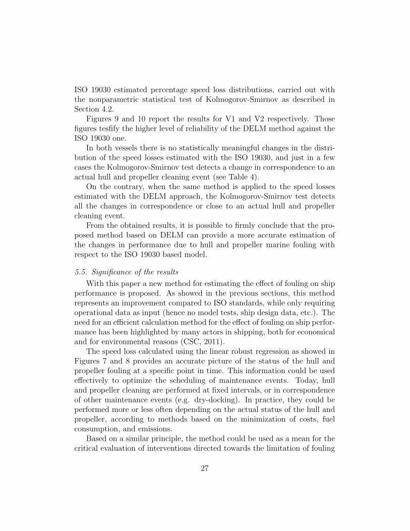
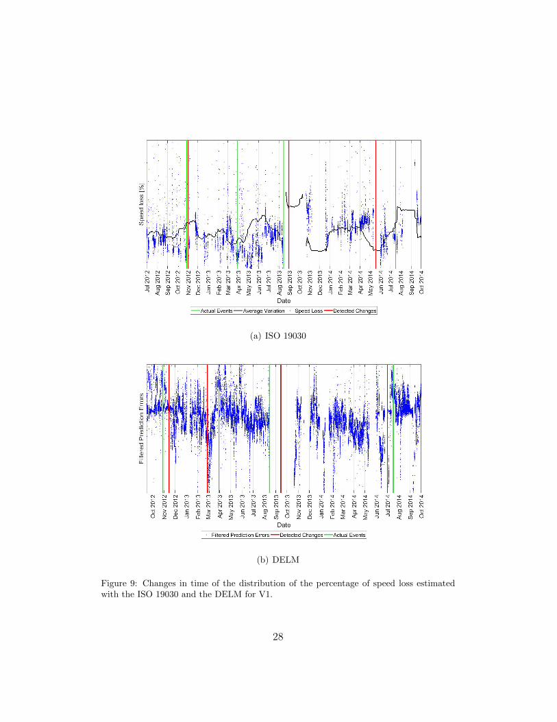
ISO 19030 estimated percentage speed loss distributions, carried out withthe nonparametric statistical test of Kolmogorov-Smirnov as described inSection 4.2.

Figures 9 and 10 report the results for V1 and V2 respectively. Thosefigures tesfify the higher level of reliability of the DELM method against theISO 19030 one.

In both vessels there is no statistically meaningful changes in the distri-bution of the speed losses estimated with the ISO 19030, and just in a fewcases the Kolmogorov-Smirnov test detects a change in correspondence to anactual hull and propeller cleaning event (see Table 4).

On the contrary, when the same method is applied to the speed lossesestimated with the DELM approach, the Kolmogorov-Smirnov test detectsall the changes in correspondence or close to an actual hull and propellercleaning event.

From the obtained results, it is possible to firmly conclude that the pro-posed method based on DELM can provide a more accurate estimation ofthe changes in performance due to hull and propeller marine fouling withrespect to the ISO 19030 based model.

5.5. Significance of the results

With this paper a new method for estimating the effect of fouling on shipperformance is proposed. As showed in the previous sections, this methodrepresents an improvement compared to ISO standards, while only requiringoperational data as input (hence no model tests, ship design data, etc.). Theneed for an efficient calculation method for the effect of fouling on ship perfor-mance has been highlighted by many actors in shipping, both for economicaland for environmental reasons (CSC, 2011).

The speed loss calculated using the linear robust regression as showed inFigures 7 and 8 provides an accurate picture of the status of the hull andpropeller fouling at a specific point in time. This information could be usedeffectively to optimize the scheduling of maintenance events. Today, hulland propeller cleaning are performed at fixed intervals, or in correspondenceof other maintenance events (e.g. dry-docking). In practice, they could beperformed more or less often depending on the actual status of the hull andpropeller, according to methods based on the minimization of costs, fuelconsumption, and emissions.

Based on a similar principle, the method could be used as a mean for thecritical evaluation of interventions directed towards the limitation of fouling

27

(a) ISO 19030

(b) DELM

Figure 9: Changes in time of the distribution of the percentage of speed loss estimatedwith the ISO 19030 and the DELM for V1.

28

(a) ISO 19030

(b) DELM

Figure 10: Changes in time of the distribution of the percentage of speed loss estimatedwith the ISO 19030 and the DELM for V2.

29

effect. Measuring the value of the speed loss before, and after, maintenanceevents can help understanding their effectiveness, and hence making more ap-propriate and informed choices. As an example, the hull cleaning performedon V2 (second maintenance event) only decreased the effect of fouling by alimited extent, while the simultaneous hull and propeller cleaning performeda few months later (third maintenance event) appeared to have a much largereffect. Similarly, the accurate estimations provided by this method could beused to evaluate the efficiency of anti-fouling paints, a widely-adopted solu-tion to reduce the effect of fouling that, however, constitutes at the sametime a cost for the company, and has a strong negative impact on the marineenvironment (Lindgren et al., 2016).

Given these premises, the ISO standard related to the estimation of ma-rine fouling (ISO 15016:2015, 2015) should be integrated with the proposedmethodology which, in presence of the conditions described in this paper, canlead to better results compared to the current methods. If widely adoptedand associated to cleaning optimization schedules, it is possible to believethat the proposed method could significantly contribute to an increase in theoperational efficiency of the global fleet, hence leading to a reduction in CO2

emissions from shipping.6. Conclusions

In this work the problem of estimating the speed loss caused by the effectof fouling on the ship hull and propeller is investigated. Since marine foulingis a phenomenon that strongly affects a ship’s regarding powering perfor-mance and its effects can be observed after just a few months of operations,the possibility of correctly estimate its impacts can improve the ability of theship operators to effectively schedule the dry-docking for cleaning the hulland the propeller.

For this purpose a two-step data-driven approach, based on the Deep Ex-treme Learning Machines which are the most advanced tools in the contextand advanced statistical methods is proposed. Thanks to such an approach, itis possible to build a Digital Twin of the ship that can be effectively exploitedto detect during real operations a deviation in the speed performances (re-spect to the ones achievable with clean hull and propeller), and consequentlyto identify the extension of the marine fouling phenomena. Then the proposalhas been compared with the state-of-the-art alternative method, namely theISO 19030 standard, using real-world data coming from two Handymax chem-ical/product tankers. Results clearly show the effectiveness of the proposal

30

and its better prediction accuracy and reliability, with respect to the ISO19030. This is shown by both a more accurate and consistent prediction ofthe loss of performance over time, between cleaning intervals, and by theability of automatically detecting maintenance events.

It has to be noted that the proposed method requires a non-indifferentamount of data in order to monitor the current speed loss, and these dataneed to be collected adopting an on-board network of sensors and persisted ona dedicated local storage. Moreover, since the predicted speed loss is subjectto local noises, mainly due to the weather and operational conditions, theglobal speed loss trend has only to be seen on a wide time-span in order tounderstand its behaviour.

Given these premises, the application of the proposed method is benefi-cial both to determine the effective intervals between maintenance actions,for propeller and hull cleaning, and to estimate ship efficiency. In the fu-ture, the proposed method could be exploited also for the evaluation of theeffectiveness of different energy-saving solutions, such as the case of a newpropeller design or the evaluation of the benefits deriving from the applica-tion of sails. The contribution of this work can be seen as a step forwardin supporting both the development of new technologies, able to improveperformances and efficiency of the ship, and the implementation of suitableCondition Based Maintenance policies for increasing the shipping sustain-ability. Moreover, the proposed method, will facilitate the verification ofthe impact of new technologies or vessel components, thereby allowing toincrease the transparency of energy and fuels efficiency technologies by pro-viding a method to validate fuel savings claims made by the manufacturersand providers, supporting further uptake in the shipping industry.

References

1. IPCC, . Global warming of 1.5°C. Tech. Rep.; Intergovernmental Panelon Climate Change; 2018. URL: http://www.ipcc.ch/report/sr15/;oCLC: 1056192590.

2. Smith, T.W.P., Jalkanen, J.P., Anderson, B.A., Corbett, J.J., Faber, J.,Hanayama, S., O’Keeffe, E., Parker, S., Johansson, L., Aldous, L.,et al. Third international maritime organization green house gas study.International Maritime Organization (IMO), London 2014;327.

31

3. Anderson, K., Bows, A.. Executing a Scharnow turn: reconciling ship-ping emissions with international commitments on climate change. CarbonManagement 2012;3(6):615–628.

4. Gilbert, P., Walsh, C., Traut, M., Kesieme, U., Pazouki, K., Murphy,A.. Assessment of full life-cycle air emissions of alternative shipping fuels.Journal of Cleaner Production 2018;172:855–866.

5. Lutzen, M., Mikkelsen, L., Jensen, S., Rasmussen, H.. Energy effi-ciency of working vessels – A framework. Journal of Cleaner Production2017;143:90–99.

6. Schim van der Loeff, W., Godar, J., Prakash, V.. A spatially explicit data-driven approach to calculating commodity-specific shipping emissions pervessel. Journal of Cleaner Production 2018;205:895–908.

7. MEPC, . Meeting Summary of the Marine Environment Protection Com-mittee (MEPC), 72nd Session. Technical Report; Maritime EnvironmentalProtection Committee (MEPC), part of the International Maritime Organ-isation (IMO); London, United Kingdom; 2018.

8. Deshpande, P.C., Kalbar, P.P., Tilwankar, A.K., Asolekar, S.R.. A novelapproach to estimating resource consumption rates and emission factorsfor ship recycling yards in alang, india. Journal of cleaner production2013;59:251–259.

9. Krozer, J., Mass, K., Kothuis, B.. Demonstration of environmentally soundand cost-effective shipping. Journal of Cleaner Production 2003;11(7):767–777.

10. Adland, R., Cariou, P., Jia, H., Wolff, F.. The energy efficiency effects ofperiodic ship hull cleaning. Journal of Cleaner Production 2018;178:1–13.

11. Calder, N.. Marine Diesel engines: Maintenance, troubleshooting, and re-pair. International Marine; 1992.

12. Psaraftis, H.N., Kontovas, C.A.. Ship speed optimization: Concepts, modelsand combined speed-routing scenarios. Transportation Research Part C:Emerging Technologies 2014;44:52–69.

32

13. Demirel, Y.K., Uzun, D., Zhang, Y., Fang, H., Day, A.H., Turan,O.. Effect of barnacle fouling on ship resistance and powering. Biofouling2017a;33(10):819–834.

14. Yebra, D., Kiil, S., Dam-Johansen, K.. Antifouling technology - past,present and future steps towards efficient and environmentally friendlyantifouling coatings. Progress in Organic Coatings 2004;50(2):75–104.

15. Lindgren, F., Wilewska-Bien, M., Granhag, L., Andersson, K., Eriksson,K.. Discharges to the sea. In: Shipping and the environment: improvingenvironmental performance in marine transportation. 2016:.

16. Schultz, M.. Frictional resistance of antifouling coating systems. Journal offluids engineering 2004;126(6):1039–1047.

17. Kempf, G.. On the effect of roughness on the resistance of ships. Trans INA1937;79:109–119.

18. Atlar, M., Glover, E.J., Candries, M., Mutton, R.J., Anderson, C.D..The effect of a foul release coating on propeller performance. In: Inter-national conference on Marine Science and Technology for EnvironmentalSustainability (ENSUS 2002). 2002:.

19. Seo, K., Atlar, M., Goo, B.. A study on the hydrodynamic effect ofbiofouling on marine propeller. Journal of The Korean Society of MarineEnvironment & Safety 2016;22(1):123–128.

20. Owen, D., Demirel, Y.K., Oguz, E., Tezdogan, T., Incecik, A.. Investi-gating the effect of biofouling on propeller characteristics using cfd. OceanEngineering 2018;159:505 – 516.

21. Candries, M., Atlar, M., Anderson, C.D.. Estimating the impact of new-generation antifoulings on ship performance: the presence of slime. Journalof Marine Engineering & Technology 2003;2(1):13–22.

22. Khor, Y.S., Xiao, Q.. CFD simulations of the effects of fouling and an-tifouling. Ocean Engineering 2011;38(10):1065–1079.

23. Lam, J.S.L., Lai, K.H.. Developing environmental sustainability by anp-qfdapproach: the case of shipping operations. Journal of Cleaner Production2015;105:275–284.

33

24. Caric, H., Klobucar, G., Stambuk, A.. Ecotoxicological risk assessment ofantifouling emissions in a cruise ship port. Journal of Cleaner Production2016;121:159–168.

25. Kjaer, L.L., Pigosso, D.C., McAloone, T.C., Birkved, M.. Guidelinesfor evaluating the environmental performance of product/service-systemsthrough life cycle assessment. Journal of Cleaner Production 2018;190:666–678.

26. CSC, . Air pollution and energy efficiency, a transparent and reliable hulland propeller performance standard. Tech. Rep.; Clean Shipping Coali-tion; 2011. URL: http://bellona.no/assets/sites/3/2015/06/fil_

MEPC_63-4-8_-_A_transparent_and_reliable_hull_and_propeller_

performance_standard_CSC1.pdf.

27. Schultz, M.P.. Effects of coating roughness and biofouling on ship resistanceand powering. Biofouling 2007;23(5):331–341.

28. Atlar, M., Yeginbayeva, I., Turkmen, S., Demirel, Y., Carchen, S.,Marino, A., Williams, D.. A rational approach to predicting the effectof fouling control systems on “in-service” ship performance. In: 3rd Inter-national Conference on Naval Architecture and Maritime, Yildiz TechnicalUniversity, Istanbul (INT-NAM 2018). 2018:.

29. Demirel, Y.K., Turan, O., Incecik, A.. Predicting the effect of biofoulingon ship resistance using cfd. Applied Ocean Research 2017b;62:100 – 118.

30. Carchen, A., Pazouki, K., Atlar, M.. A rational approach to predictingthe effect of fouling control systems on “in-service” ship performance. In:Hull Performance and Insight Conference (HullPIC). 2017:.

31. Stevens, E.. The increase in frictional resistance due to the action of wateron bottom paint. Naval Engineers Journal 1937;49(4):585–588.

32. ISO 19030-2. Ships and marine technology Measurement of changes in hulland propeller performance - Part 2: Default method. Standard; Interna-tional Organization for Standardization; Geneva, CH; 2016.

33. Koboevic, Z., Bebic, D., Kurtela, Z.. New approach to monitoring hullcondition of ships as objective for selecting optimal docking period. Shipsand Offshore Structures 2018;0(0):1–9.

34

34. ISO 19030-1. Ships and marine technology Measurement of changes in hulland propeller performance - Part 1: General principles. Standard; Inter-national Organization for Standardization; Geneva, CH; 2016.

35. ISO 19030-3. Ships and marine technology Measurement of changes in hulland propeller performance - Part 3: Alternative methods. Standard; In-ternational Organization for Standardization; Geneva, CH; 2016.

36. Logan, K.P.. Using a ship’s propeller for hull condition monitoring. NavalEngineers Journal 2012;124(1):71–87.

37. Bialystocki, N., Konovessis, D.. On the estimation of ship’s fuel consump-tion and speed curve: A statistical approach. Journal of Ocean Engineeringand Science 2016;1(2):157–166.

38. Foteinos, M., Tzanos, E., Kyrtatos, N.. Ship hull fouling estimationusing shipboard measurements, models for resistance components, andshaft torque calculation using engine model. Journal of Ship Research2017;61(2):64–74.

39. Cipollini, F., Oneto, L., Coraddu, A., Murphy, A.J., Anguita, D..Condition-based maintenance of naval propulsion systems with superviseddata analysis. Ocean Engineering 2018;149:268–278.

40. Oneto, L., Coraddu, A., Sanetti, P., Karpenko, O., Cipollini, F., Cleophas,T., Anguita, D.. Marine safety and data analytics: Vessel crash stop ma-neuvering performance prediction. In: International Conference on Arti-ficial Neural Networks. 2017a:.

41. Coraddu, A., Oneto, L., Ghio, A., Savio, S., Anguita, D., Figari, M..Machine learning approaches for improving condition-based maintenanceof naval propulsion plants. Proceedings of the Institution of MechanicalEngineers, Part M: Journal of Engineering for the Maritime Environment2016;230(1):136–153.

42. Parlak, A., Islamoglu, Y., Yasar, H., Egrisogut, A.. Application of artificialneural network to predict specific fuel consumption and exhaust temper-ature for a diesel engine. Applied Thermal Engineering 2006;26(8):824 –828.

35

43. Pedersen, B.P., Larsen, J.. Prediction of full-scale propulsion power usingartificial neural networks. In: The 8th International Conference Computerand IT Applications in the Maritime Industries. 2009:.

44. Petersen, J.P., Jacobsen, D.J., Winther, O.. Statistical modelling forship propulsion efficiency. Journal of marine science and technology2012;17(1):30–39.

45. Radonjic, A., Vukadinovic, K.. Application of ensemble neural networksto prediction of towboat shaft power. Journal of Marine Science andTechnology 2015;20(1):64–80.

46. Jonge, C.d.. Data-driven analysis of vessel performance. Master’s thesis;NTNU; 2017.

47. Leifsson, L., Sævarsdottir, H., Sigurdhsson, S., Vesteinsson, A.. Grey-box modeling of an ocean vessel for operational optimization. SimulationModelling Practice and Theory 2008;16(8):923–932.

48. Kasun, L.L.C., Zhou, H., Huang, G.B., Vong, C.M.. Representationallearning with elms for big data. IEEE Intelligent Systems 2013;28(6):31–34.

49. Cambria, E., Huang, G.B.. Extreme learning machines. IEEE IntelligentSystems 2013;28(6):30–59.

50. Huang, G., Huang, G.B., Song, S., You, K.. Trends in extreme learningmachines: A review. Neural Networks 2015;61:32–48.

51. Huang, G.B., Zhu, Q.Y., Siew, C.K.. Extreme learning machine: Theoryand applications. Neurocomputing 2006a;70(1):489–501.

52. Huang, G.B.. An insight into extreme learning machines: random neurons,random features and kernels. Cognitive Computation 2014;6(3):376–390.

53. Huang, G.B.. What are extreme learning machines? filling the gap be-tween frank rosenblatt’s dream and john von neumann’s puzzle. CognitiveComputation 2015;7(3):263–278.

54. Ridella, S., Rovetta, S., Zunino, R.. Circular backpropagation networks forclassification. IEEE Transactions on Neural Networks 1997;8(1):84–97.

36

55. Rumelhart, D.E., Hinton, G.E., Williams, R.J.. Learning representationsby back-propagating errors. Cognitive modeling 1988;5(3):1.

56. Huang, G.B., Li, M.B., Chen, L., Siew, C.K.. Incremental ex-treme learning machine with fully complex hidden nodes. Neurocomputing2008;71(4):576–583.

57. Huang, G.B., Chen, L., Siew, C.K.. Universal approximation using in-cremental constructive feedforward networks with random hidden nodes.IEEE Transactions on Neural Networks 2006b;17(4):879–892.

58. Huang, G.B., Zhu, Q.Y., Siew, C.K.. Extreme learning machine: a newlearning scheme of feedforward neural networks. In: IEEE InternationalJoint Conference on Neural Networks. 2004:.

59. Bengio, Y., Courville, A., Vincent, P.. Representation learning: A reviewand new perspectives. IEEE transactions on pattern analysis and machineintelligence 2013;35(8):1798–1828.

60. Vincent, P., Larochelle, H., Bengio, Y., Manzagol, P.A.. Extracting andcomposing robust features with denoising autoencoders. In: Internationalconference on Machine learning. 2008:.

61. Zhou, H., Huang, G.B., Lin, Z., Wang, H., Soh, Y.C.. Stacked extremelearning machines. IEEE Transactions on Cybernetics 2015;45(9):2013–2025.

62. Tissera, M.D., McDonnell, M.D.. Deep extreme learning machines: su-pervised autoencoding architecture for classification. Neurocomputing2016;174:42–49.

63. Oneto, L., Fumeo, E., Clerico, C., Canepa, R., Papa, F., Dambra, C.,Mazzino, N., D., A.. Dynamic delay predictions for large-scale railwaynetworks: Deep and shallow extreme learning machines tuned via thresh-oldout. IEEE Transactions on Systems, Man and Cybernetics: Systems2017b;47(10):2754 – 2767.

64. Glaessgen, E., Stargel, D.. The digital twin paradigm for future nasa and usair force vehicles. In: 53rd Structures, Structural Dynamics and MaterialsConference. 2012:.

37

65. Boschert, S., Rosen, R.. Digital twin—the simulation aspect. In: Mecha-tronic Futures. 2016:.

66. Zhao, Y., Sun, J.. Robust truncated support vector regression. ExpertSystems with Applications 2010;37(7):5126–5133.

67. Smirnov, N.V.. Approximate laws of distribution of random variables fromempirical data. Uspekhi Matematicheskikh Nauk 1944;(10):179–206.

68. ISO 15016:2015. Ships and marine technology - guidelines for the assessmentof speed and power performance by analysis of speed trial data. Standard;International Organization for Standardization; Geneva, CH; 2015.

69. Chauvenet, W.. A Manual of Spherical and Practical Astronomy. Lippincott;1863.

70. Glaisher, J.W.L.. On a class of definite integrals. The London, Ed-inburgh, and Dublin Philosophical Magazine and Journal of Science1871;42(280):294–302.

71. Fujiwara, T., Ueno, M., Ikeda, Y.. Cruising Performance of a LargePassenger Ship In Heavy Sea. In: The Sixteenth International Offshoreand Polar Engineering Conference. 2006:.

72. Vapnik, V.N.. Statistical learning theory. Wiley New York; 1998.

73. Coraddu, A., Oneto, L., Ghio, A., Savio, S., Figari, M., Anguita, D..Machine learning for wear forecasting of naval assets for condition-basedmaintenance applications. In: Electrical Systems for Aircraft, Railway,Ship Propulsion and Road Vehicles (ESARS), 2015 International Confer-ence on. 2015:.

74. Rosasco, L., De Vito, E., Caponnetto, A., Piana, M., Verri, A.. Are lossfunctions all the same? Neural Computation 2004;16(5):1063–1076.

75. Caponnetto, A., De Vito, E.. Optimal rates for the regularized least-squaresalgorithm. Foundations of Computational Mathematics 2007;7(3):331–368.

76. Oneto, L.. Model selection and error estimation without the agonizing pain.WIREs Data Mining and Knowledge Discovery 2018;.

38

77. Tibshirani, R.. Regression shrinkage and selection via the lasso. Journal ofthe Royal Statistical Society Series B (Methodological) 1996;58(1):267–288.

78. Zou, H., Hastie, T.. Regularization and variable selection via the elastic net.Journal of the Royal Statistical Society: Series B (Statistical Methodology)2005;67(2):301–320.

79. Tang, J., Deng, C., Huang, G.. Extreme learning machine for multilayerperceptron. IEEE transactions on neural networks and learning systems2016;27(4):809–821.

80. Coraddu, A., Oneto, L., Baldi, F., Anguita, D.. Vessels fuel consump-tion forecast and trim optimisation: A data analytics perspective. OceanEngineering 2017;130:351–370.

39