data fusion for improved toa/tdoa position determination in

Data Fusion For Improved TOA/TDOA Position Determination in Wireless Systems

by

Rahman I. Reza

Thesis submitted to the Faculty of the Virginia Polytechnic Institute and State University

in partial fulfillment of the requirements for the degree of

MASTER OF SCIENCE in

Electrical Engineering

Approved:

___________________ _________________________

Dr. Brian D. Woerner Dr. Amy E. Bell (Co-Chair) (Co- Chair)

_____________________________

Dr. Tim Pratt

July 2000 Blacksburg, Virginia

Key Words: Position Location, TDOA, TOA, Data Fusion Architecture, NLOS

Data Fusion For Improved TOA/TDOA Position Determination in Wireless Systems

by Rahman I. Reza

Committee Chair: Dr. Brian D. Woerner Co-Chair: Dr. Amy E. Bell

Electrical Engineering

Abstract The Federal Communications Commission (FCC) that regulates all wireless communication service providers has issued modified regulations that all service providers must select a method for providing position location (PL) information of a user, requesting for E-911 service, by October 2000. The wireless 911 rules adopted by the FCC are aimed both for improving the reliability of the wireless 911 services and for providing the enhanced features generally available for wireline calls. From the service providers� perspective, effective position location technologies must be utilized to meet the FCC rules. The Time-of-Arrival (TOA) and the Time-Difference-of-Arrival (TDOA) methods are the technology that can provide accurate PL information without necessitating excessive hardware or software changes to the existing cellular/PCS infrastructure. The TOA method works well when the mobile station (MS) is located close to the controlling base station. With certain corrections applied, the TOA method can perform reliably even in the presence of Non-Line-of-Sight (NLOS) condition. The TDOA method performs better when the MS is located at a significant distance from the controlling base station. However, under the NLOS environmental condition, the performance of the TDOA method degenerates significantly. The fusion of TOA and the TDOA method exhibits certain advantages that are not evident when only one of the methods is applied. This thesis investigates the performance of data fusion techniques for a PL system, that are able to merge independent estimates obtained from TOA and TDOA measurements. A channel model is formulated for evaluating PL techniques within a NLOS cellular environment. It is shown that NLOS propagation can introduce a bias into TDOA measurements. A correction method is proposed for removing this bias and new corrected data fusion techniques are compared with previous techniques using simulation method, yielding favorable results.

iii

Acknowledgement

A number of people have contributed to the successful completion of this research work. Many

have given their direct efforts to the preparation of this report. I would like to render my gratitude

to each one of them.

I am greatly in debt to my venerable advisor Dr. Brian D. Woerner for giving me the opportunity to

work on this project. His valuable suggestions and generous support provided me the necessary

guidance to complete the research work. He was more than only an advisor to me. I cannot imagine

anyone else who could be a better research advisor than him.

I am also in debt to my co-advisor Dr. Amy E. Bell for her constant encouragement, suggestions

and assistance for preparing this report. It would be a great lapse if I don�t acknowledge that without

her complete assistance and full support; it would not have been possible for me to prepare this

report in its present manner.

I would also like to show my great sense of gratitude to Dr. Tim Pratt for his precious suggestions

and guidance from time to time.

I thank the Bradley Department of Electrical Engineering for the generous financial assistance to

this research effort.

I am grateful to all the members of the Mobile and Portable Radio Research Group (MPRG) for

their assistance during the tenure of this research work. Special thanks to the MPRG staff members

who have rendered direct assistance throughout the research work.

I have no words to say how much grateful I am to my beloved wife Rumman Wazed for her

sacrifice and understanding during the duration of this research work. It is she who always propelled

me to conquer any hindrance ever since our marriage.

Finally, I would like to express my deep gratitude to my parents without whose blessings it were not

possible for me to see even a single sparkle of light in this beautiful world.

iv

Contents Abstract ................................................................................................................. ii Acknowledgement ...............................................................................................iii Introduction...........................................................................................................1

1.1 The Need for Location Information in Wireless Systems ........................................................ 1

1.2 Overview of Different Position Location Methods................................................................... 3 1.2.1 Modified Handset Techniques .................................................................................................................3 1.2.2 Unmodified Handset Techniques............................................................................................................4

1.3 Research Outline ............................................................................................................................. 6 1.3.1 Purpose of Research ..................................................................................................................................6 1.3.2 Thesis Outline.............................................................................................................................................7

Position Determination: Principles and Algorithms ........................................... 8 2.1 Time of Arrival (TOA) Techniques ............................................................................................. 8

2.1.1 Mathematical model of TOA measurements.........................................................................................9 2.1.2 Correction of TOA Measurements in NLOS......................................................................................11 2.1.3 TOA Procedure for E-911......................................................................................................................11 2.1.4 Taylor Series Method used for TOA PL System ................................................................................12

2.2 Time Difference of Arrival (TDOA) PL Technique ............................................................... 13 2.2.1 Mathematical Model for Hyperbolic Position Location ....................................................................15 2.2.2 Application of TDOA to the Cellular E-911 Problem ......................................................................16 2.2.3 Mathematical Procedure for Taylor-Series Method............................................................................16 2.2.4 Mathematical Model for TDOA Equations in Chan�s Method........................................................18

2.3 Measure of PL Estimator Performance..................................................................................... 18 2.3.1 Circular Error Probability (CEP)...........................................................................................................19 2.3.2 Geometric Dilution of Precision (GDOP) ..........................................................................................19 2.3.3 Mean Square Error (MSE)......................................................................................................................20 2.3.4 Cramer-Rao Lower Bound .....................................................................................................................20

2.4 Chapter Summary.......................................................................................................................... 21

Data Fusion ........................................................................................................ 22 3.1 JDL Data Fusion Architecture.................................................................................................... 22

3.2 Data Fusion Model for Position Location Estimation............................................................ 24

v

3.2.1 First Level Data Fusion...........................................................................................................................26 3.2.2 Second Level Data Fusion......................................................................................................................26 3.2.3 Level Four Data Fusion: The final choice............................................................................................27

3.3 Chapter Summary.......................................................................................................................... 28

The Channel Models .......................................................................................... 29 4.1 Received Signal Models................................................................................................................ 29

4.1.1 TOA Received Signal Model ..................................................................................................................29 4.1.2 TDOA Received Signal Model...............................................................................................................32

4.2 Path Loss Model............................................................................................................................ 34

4.3 Additive White Gaussian Noise (AWGN) Channel ................................................................ 35

4.4 Chapter Summary.......................................................................................................................... 36

Data Fusion With Uncorrected TDOA.............................................................. 37 5.1 Simulation Models ........................................................................................................................ 37

5.2 Validation of TOA Simulator Performance.............................................................................. 41 5.2.1 Mobile Trajectory Estimation ................................................................................................................41 5.2.2 Evaluation of the Estimator�s Performance for Position Estimation .............................................46

5.3 Validation of TDOA Simulator Performance .......................................................................... 47 5.3.1 Mobile Trajectory Estimation ................................................................................................................49 5.3.2 Evaluation of the Estimator�s Performance for Position Estimation .............................................52

5.4 Implementation of Data Fusion Model in Position Location................................................ 54

5.5 Chapter Summary ��...58

TDOA Data Model and Extension of Wylie-Holtzman Algorithm to TDOA Ranges ............................................................................................... 60

6.1 Data Model for TDOA Range Measurements ......................................................................... 60 6.2 Simulation Model .......................................................................................................................... 62

6.3 Correction of TDOA Range Measurements Biased by NLOS Error................................... 62 6.3.1 Identification of NLOS Bias in TDOA Range Measurements.........................................................62 6.3.2 Extension of the Wylie-Holtzman Algorithm to the TDOA Range Measurements ....................63 6.3.3 Proposed Correction Method ................................................................................................................66

6.4 Validation of Correction Method Applied to TDOA Measurements................................... 66 6.4.1 Mobile Trajectory Estimation ................................................................................................................67 6.4.2 TDOA PL Estimator�s Performance with Corrected TDOA Measurements ...............................68

6.5 Data Fusion Architecture with Corrected TDOA Measurements ........................................ 72

vi

Conclusions ........................................................................................................ 84 7.1 Summary of Results ...................................................................................................................... 84

7.2 Contributions of this Research Work ........................................................................................ 86

7.3 Directions for Future Research................................................................................................... 88

Bibliography ....................................................................................................... 90

Vita ...................................................................................................................... 93

vii

List of Tables Table 5.1: Standard Deviation of TOA Measurements from Smoothed Curves .....................43

Table 5.2: Standard Deviation of TOA Measurements from Smoothed Curves.....................43

Table 5.3: TOA Estimator Performance on Mobile Trajectory Estimation ...........................45

Table 5.4: TOA Estimator Performance at Different Mobile Location ..................................47

Table 5.5: Standard Deviation of TDOA Range Measurements from Smoothed Curve ........50


Table 5.7: TDOA Estimator Performance at Different Mobile Location ...............................52

Table 5.8: TDOA Estimator�s Performance When MS is Very Close to the Controlling BS..53

Table 5.9: Estimators� Output in Data Fusion Architecture at MS (600, 900) ........................55

Table 5.10: Estimators� Output in Data Fusion Architecture at MS (2000, 2000)...................56

Table 5.11: Estimators� Output in Data Fusion Architecture at MS (600, 2500).....................57

Table 5.12: Estimators� Output with Unbiased Input at MS (25, 25)......................................58

Table 5.13: Estimators� Output with Unbiased Input at MS (150, 150)...................................59


Table 6.2: TDOA Estimator Performance at Different Mobile Location ...............................71


Table 6.4: Estimators� Output in Data Fusion Architecture at MS (2000, 2000) ....................74

Table 6.5: Estimators� Output in Data Fusion Architecture at MS (600, 2500) ......................75

Table 6.6: Estimators� Output in Data Fusion Architecture at MS (50, 50)............................76


Table 6.8: Data Fusion Architecture Performance at MS (600, 900) with all BS having NLOS..........................................................................................................78

Table 6.9: Data Fusion Architecture Performance at MS (2000,2000) with all BS having NLOS..........................................................................................................79

Table 6.10: Data Fusion Architecture Performance at MS (600,2500) with all BS having NLOS.........................................................................................................80

Table 6.11: Data Fusion Architecture Performance at MS (600,2500) in GCC with 25 dB SNR .....................................................................................................81

viii



ix

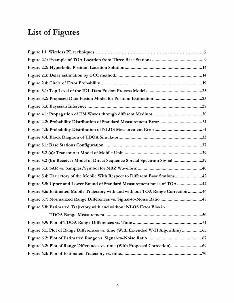
List of Figures

Figure 1.1: Wireless PL techniques ��. 6

Figure 2.1: Example of TOA Location from Three Base Stations ........................................... 9

Figure 2.2: Hyperbolic Position Location Solution.................................................................14

Figure 2.3: Delay estimation by GCC method.........................................................................14

Figure 2.4: Circle of Error Probability .....................................................................................19

Figure 3.1: Top Level of the JDL Data Fusion Process Model ...............................................23

Figure 3.2: Proposed Data Fusion Model for Position Estimation.........................................25

Figure 3.3: Bayesian Inference ................................................................................................27

Figure 4.1: Propagation of EM Waves through different Medium .........................................30

Figure 4.2: Probability Distribution of Standard Measurement Error ....................................31

Figure 4.3: Probability Distribution of NLOS Measurement Error........................................31

Figure 4.4: Block Diagram of TDOA Simulator......................................................................33

Figure 5.1: Base Stations Configuration ..................................................................................37

Figure 5.2 (a): Transmitter Model of Mobile Unit ..................................................................39

Figure 5.2 (b): Receiver Model of Direct Sequence Spread Spectrum Signal.........................39

Figure 5.3: SAR vs. Samples/Symbol for NRZ Waveform......................................................40

Figure 5.4: Trajectory of the Mobile With Respect to Different Base Stations.......................42

Figure 5.5: Upper and Lower Bound of Standard Measurement noise of TOA .....................44

Figure 5.6: Estimated Mobile Trajectory with and with out TOA Range Correction ............46

Figure 5.7: Normalized Range Differences vs. Signal-to-Noise Ratio ...................................48

Figure 5.8: Estimated Trajectory with and without NLOS Error Bias in TDOA Range Measurement .................................................................................50

Figure 5.9: Plot of TDOA Range Differences vs. Time ..........................................................51

Figure 6.1: Plot of Range Differences vs. time (With Extended W-H Algorithm) .................65

Figure 6.2: Plot of Estimated Range vs. Signal-to-Noise Ratio..............................................67

Figure 6.2: Plot of Range Differences vs. time (With Proposed Correction) ..........................69

Figure 6.3: Plot of Estimated Trajectory vs. time....................................................................70

1

Chapter 1

Introduction

Position estimation of mobile users in cellular phone networks is becoming more important as the

numbers of emergency calls originating from mobile telephone units increase. New Personal

Communication Systems (PCS) are introducing new data and voice services [30]; however, the

present wireless radio systems are still unable to provide accurate mobile user position location (PL)

information to the Public Safety Answering Points (PSAP). This problem of providing reliable and

accurate PL of mobile units in wireless communication systems has drawn considerable attention in

the recent years as the deadline mentioned in a regulation adopted by the Federal Communication

Commission is impending. Current regulation states that, by the October 2000 all the wireless

carriers will have to identify a method for determining the location of the mobile unit making a E-

911 call within a radius of no more than 125 meters rms [9]. Depending on the method selected, the

accuracy requirements may be even more stringent, and hardware must be deployed over the next

one to four years. This chapter discusses the motivation behind position determination requirements

for mobile users in cellular system, an overview of different radio frequency based position location

methods, and an outline of the research work contained in this thesis.

1.1 The Need for Location Information in Wireless Systems In case of landline phones, the E-911 service provides the Public Safety Answering Point (PSAP)

the number of the calling party. The Automated Number Identification (ANI) information enables

the call back capability in case the emergency call is disconnected. A complete E-911 service not

only provides the ANI but also enables the PSAP to identify an emergency call originating address

through the use of an Automated Location Identification (ALI) database.

For the mobile users, although it is possible to identify the cell from where the E-911 call has been

generated, it is not yet possible to identify the exact position in the cell from where the emergency

call has been made.

In mid 90�s, the Federal Communications Commission (FCC) addressed this problem

issuing regulations outlining three staged phases, which all the wireless service providers must

2

implement to provide the capability of universally available E-911 service with position

determination.

The original regulation state that, in the first phase the wireless service providers have to

achieve the capability to transmit Mobile Identification Number (MIN) of the handset generating 9-

1-1 call to the PSAP without any interception by the carrier for credit checks or other validation

process. Time frame allocated for this service was twelve months from the effective date of FCC

rule, June 1996. In the second phase, the wireless service providers must provide a cell-site location

mechanism in their wireless system along with providing the PSAP with the caller�s phone number.

In the third phase, the wireless service providers will have to achieve the target of identifying the

location of the mobile users, attempted 9-1-1 calls, within a circle of radius of no more than 125

meters in at least 67 percent of all the cases [9]. The FCC regulation requires that all the wireless

carriers achieve this goal by October 1, 2001.

In October 1999, the FCC revised its phase II requirements, offering service providers two

alternative methods for position determination. Carriers have until October 1, 2000 to declare

whether they will offer a network based or handset based solution to the position determination

problem. For carriers offering network based solutions, an accuracy requirement specifies that, 67

percent of E-911 calls must be located with 100 meters, and 95 percent of E-911 calls must be

located with 300 meters. This service must be available to 50% of the network within 6 months of a

PSAP request and available to 100% of the network within 18 months of a PSAP request.

For carriers opting for a handset-based approach, accuracy requirements are 50 meters for

67% of the calls and 150 meters for 95% of the calls. Carriers providing handset-based position

determination must begin selling phones with location technology by March 1, 2001, and must

switch all subscriber equipment to enable location by December 31, 2004.

At least two commercial developers (U.S. Wireless and True Position) offer network-based

solutions to position determination. Service providers opting for handset-based solutions will likely

embed low cost Global Position System (GPS) receivers in their handsets [31]. Although it is not yet

apparent which approach the industry will adopt, this thesis addresses the network-based approach.

Although the deadline for providing the PL service is imminent, no single wireless service provider

is even near to meet the requirements. Significant research work is aimed at finding a proven

method to implement a measurement and to estimate the system without bringing in too much

hardware or software modification in the existing cellular infrastructure.

3

1.2 Overview of Different Position Location Methods There are a number of different radio frequency based techniques that can be used for wireless

position location. The issue is, how effectively and efficiently a technique can be implemented so

that it can be incorporated in the existing system easily without making major changes, either at the

user end or at the service provider�s end? Electromagnetic waves at radio frequency (RF) have the

unique property of traveling through most objects. PL using radio frequency is performed by direct

measurement of radio signals traveling between the base station and the mobile unit. The RF signal

reflection and obstructed line of sight introduce error in the calculated location. However, only the

radio frequency estimation systems offer the advantages of low cost, ease of integration and ability

to work in harsh environmental conditions. Therefore, RF techniques that are practically viable for

cellular systems are discussed below. The techniques can be broadly classified into two categories,

namely:

• Modified Handset Techniques

• Unmodified Handset Techniques

1.2.1 Modified Handset Techniques From the technical aspect, the modified handset techniques are easy to implement and accurate to

determine a mobile location. The GPS-based position location, mobile-assisted Time of Arrival

(TOA) technique and mobile-assisted Time Difference of Arrival (TDOA) techniques fall into this

category. The GPS-based PL requires installation of a GPS receiver in the handset and transmitting

the received GPS data on the reverse link to the base station (BS) for further processing and

position determination [13]. The drawbacks of this technique include an increase in the size and

weight of the handsets, and additional drain of the batteries in the mobile phones. Moreover, a GPS

receiver needs to have at least four satellites constantly visible. In a heavily shadowed and covered

urban environment, the line-of-sight between the mobile station and the satellites is impeded.

Therefore, the GPS based solution is a feasible option for outdoor mobile units but not for indoor

mobile units or units within urban canyons. In the mobile assisted TOA technique, the handset

stamps the current time on any outgoing signal in the reverse channel. The base station determines

the time required by the signal to reach the base station, and from that determines the distance

between the base station and the mobile unit. If at least three base stations take part in this process

then the triangulation method can be used to determine the mobile position. This requires that the

mobile station and the base stations must be accurately synchronized. Although this is not

4

impossible to achieve, it is not cost effective. The modified handset TDOA method proposed for

the CDMA system utilizes the pilot tones transmitted by different base stations. Higher power

transmission of the pilot tone allows extremely accurate tracking of the received signal. Since each

cell site transmits a Pseudo Noise (PN) code with a unique code sequence, a mobile can differentiate

each cell site�s pilot tone. The mobile measures the arrival time differences of at least three pilot

tones transmitted by three different cells. This gives rise to hyperbolic equations and by intersecting

the hyperbolas, an estimation of the mobile unit�s position can be found [10]. The estimation can

then be transmitted back to the base station through reverse channel. Since all the processing must

be done in the handset, additional hardware requirements are imposed on the handset.

1.2.2 Unmodified Handset Techniques An unmodified handset solution requires that all the modifications will be made at the base stations

and at the switching centers, thus allowing existing terminal equipment to be used. Prominent

options include: Angle of Arrival (AOA), Time of Arrival (TOA) or Direction of Arrival (DOA),

and Time Difference of Arrival (TDOA) techniques. It is also possible to combine two or more of

these techniques to achieve a more accurate position location. Combined methods are commonly

known as Hybrid Techniques [6].

The AOA method utilizes antenna-arrays to estimate the direction of arrival of the signal of

interest. A single AOA measurement constrains the source along a line. The position of the signal

source can be located at the intersection of two lines if two DOA estimates are available from two

separate antennas. Although the basic principle of the AOA method seems very simple, the method

has some drawbacks. For measurement accuracy, it is important that the mobile unit and the

participating base stations all have Line-Of-Sight (LOS) to the mobile. This is not the usual case in

cellular systems. Cellular systems have heavily shadowed channels like the ones encountered in

urban environments.

In the unmodified handset TOA technique, when a base station detects a 9-1-1 user, it

transmits a particular command or instruction signal to the user and asks the user to respond to that

command signal. The total time elapsed between the transmission of the command signal and the

reception of the acknowledgement signal is recorded at the base station. The measured round trip

delay includes the propagation delay of the signal traveling in both directions, plus a processing delay

and a response delay of the mobile handset. Therefore, if the delays associated with the handset

were known, then subtracting the values from the measured round trip delay (RTD) time would give

5

the RTD with sufficient accuracy. If two additional base stations take part in this process then the

triangulation method can be used to find the position of the user at the intersection of the circles

determined by the time delay measurements. Since this method relies on a time reference, it is highly

susceptible to the timing error due to Non-Line-Of-Sight (NLOS) between the base station and the

mobile unit.

The unmodified handset TDOA has the relative advantage over TOA in the sense that the

TDOA does not require any time reference for determining RTD. The TDOA technique estimates

the time difference of arrival of the signal from the source at multiple base stations. Two versions of

the received signal at pairs of the base stations are cross-correlated. From the peak of this cross-

correlator output, the time difference of the signal arriving at two base stations is determined. This

time difference gives rise to a hyperbola between the two receivers. If the base stations and the

mobile user are in the same plane, then the mobile lies on a line of the hyperbola. If another base

station takes part in this process, another hyperbola is defined, and the intersection of the

hyperbolas results in the position estimate of the source. The TDOA method is also referred as the

Hyperbolic Position Location method. The advantage of this technique is that all processing takes

place at the base station infrastructure level. Advantages of the method include: cost effectiveness,

no need for an absolute time reference, capability with inexpensive antennas, and immunity to

timing errors [10]. Any timing bias will be cancelled in the time difference operation. As a result, the

TDOA methods work better than the TOA methods in the absence of LOS between base stations

and the mobile unit [6].

In the hybrid techniques (HT), two or more of the techniques discussed earlier are combined

to create a more accurate position location service. When AOA and TDOA are combined to form

AOA-TDOA HT, multiple base stations receive signals from the mobile unit and the AOA

estimates from each base station; and the TDOA estimates between multiple base stations are

combined to determine target location. This type of method results in highly accurate position

determination. However care must be taken that error from one method does not affect the overall

position estimation. The AOA-TOA HT is most suitable when only one base station is able to

receive the signal from the mobile [11]. Although this technique may not be as accurate as the AOA-

TDOA HT, it may be the only unmodified handset PL solution possible when only one base station

is able to receive the mobile signal [6].

6

This thesis focuses on the use of data fusion techniques to allow efficient combining of

position determination data within hybrid schemes. Note that, data fusion is more than simple

averaging of estimates, but takes into account the quality of the various estimates.

1.3 Research Outline 1.3.1 Purpose of Research This research has two main objectives. First, we develop a model for the TDOA range

measurements and to propose an algorithm that corrects the error of the range measurements in the

TDOA method, in the absence of complete LOS between the base station and the mobile unit.

Although a timing bias may be cancelled in the TDOA technique, additional timing delay due to

NLOS propagation may still result in an erroneous solution. This research identifies a method to

make an acceptable correction to the error introduced in the range measurements due to NLOS

propagation between the base and the mobile. We propose an algorithm and validate the

implementation of this algorithm under simple channel conditions and typical base station

topographies. The second objective of this research work is to apply the data model and the

correction algorithm to the Data Fusion Architecture for the PL problem proposed by Kleine-

Figure 1.1: Wireless PL techniques

GPSBased

MobileAssited

TOA

MobileAssitedTDOA

ModifiedHandset

Techniques

AOA TOA TDOA

AOA/TOA AOA/TDOA

HybridTechniques

UnmodifiedHandset

Techniques

Position LocationTechniques

7

Ostmann and Bell [23], and to validate the decision criterion for choosing the best estimate at level

four of the data fusion model by simulation results.

1.3.2 Thesis Outline This chapter provides an introduction to the position location problem and briefly discusses the

different techniques considered to be the possible solution to the problem. Chapter 2 develops the

TOA and the TDOA methods with greater mathematical rigor, presenting algorithmic descriptions

of the two techniques. Chapter 3 gives an introduction to the Data Fusion Architecture and its

application to the position location problem. Chapter 4 describes the different channel models used

in the simulation, and Chapter 5 presents various simulation results based on this algorithm. Chapter

6 proposes the algorithm for error correction in TDOA range measurements due to Non-Line-Of-

Sight, and presents some simulation results based on this algorithm. Finally, Chapter 7 concludes the

thesis by discussing the outcomes and identifying some areas for further investigation and research

work.

8

Chapter 2

Position Determination: Principles and Algorithms Chapter 1 briefly described several position location (PL) technologies that are possible solutions to

the mobile radio PL problems. This thesis will focus on the range-based techniques of TOA and

TDOA. Because of the relative advantages of TOA and TDOA methods over other methods, these

two techniques are widely used in RF PL system for the geo-location of mobile users. Therefore the

basic principle and algorithm of only these two techniques are rigorously described in this chapter.

2.1 Time of Arrival (TOA) Techniques The Time of Arrival technique exploits triangulation to determine positions of the mobile users.

Position estimation by the triangulation is based on knowing the distance from the mobile to at least

three base stations in the line of sight (LOS). The base stations determine the time signal takes from

the source to the receiver either on the uplink or on the downlink. When 9-1-1 is dialed from a

mobile unit, the controlling base station prompts the mobile to respond to a initial signal. The total

time elapsed from the instant the command is transmitted to the instant the mobile responds is

detected. This time consists of the sum of the round trip signal delay, and any processing and

response delay within the mobile unit. When the processing delay is subtracted from the total

measured time, total round trip delay is found. Half of the quantity would be the estimate of the

signal in one direction. Multiplying this time with the traveling velocity of the electromagnetic waves

would give the approximate distance of the mobile from the base station. The approximate distance

to the mobile determined by two additional receivers could be used to determine the mobile position

at the intersection of circles from multiple TOA measurements, as illustrated in Figure 2.1.

The mobile position can be determined accurately if there exists a complete LOS between

the mobile station (MS) and the base stations. However the occurrence of non-line-of-sight (NLOS)

propagation causes the signal to take a longer path to the base station receiver and the measured

TOA is generally larger than the arrival time of an LOS signal. In such a circumstance, there is a

9

need to detect NLOS and to correct the biased error in the TOA measurements before processing

them.

2.1.1 Mathematical model of TOA measurements TOA measurements can be interpreted as the range measurements between MS and BS [2]. The

range measurements obtained from the arrival times are,

TOATOA tcr ∆=

Where,

arrivalofTimetMeasuremenRanger

mlightofSpeedWaveneticElectromagofSpeedc

TOA

TOA

=∆=

×=== sec/103 8

The range measurements can be modeled as,

),()()()( imimimimTOA tNLOStntLtrr ++== (2.1)

Figure 2.1: Example of TOA Location from Three Base Stations

rBS

r2BS

r3

BS

M

y

x

10

where,

sight-of-line-Non todueError errort measuremen Standard

BS and MSbetween distance True ttimedifferent at tsmeasuremen ofNumber

)1.....(2,1,0index timeSample....2,1index BS

i

===

=−==

==

m

m

m

NLOSnLK

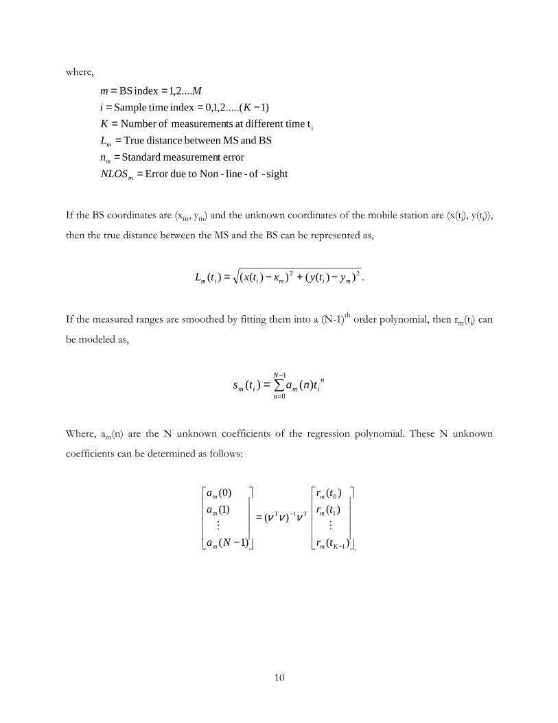
KiMm

If the BS coordinates are (xm, ym) and the unknown coordinates of the mobile station are (x(ti), y(ti)),

then the true distance between the MS and the BS can be represented as,

.))(())(()( 22mimiim ytyxtxtL −+−=

If the measured ranges are smoothed by fitting them into a (N-1)th order polynomial, then rm(ti) can

be modeled as,

∑−

==

1

0)()(

N

n

nimim tnats

Where, am(n) are the N unknown coefficients of the regression polynomial. These N unknown

coefficients can be determined as follows:

,1

1

0

1

)(

)()(

)(

)1(

)1()0(

=

− −

−

Km

m

m

TT

m

m

m

tr

trtr

Na

aa

MMννν

11

where,

.11

21

11

01

10

20

10

00

Matrix t Coefficien

==−−−−−

−

NKKKK

N

tttt

tttt

LL

MLLMMM

LL

ν

It should be noted here that the standard error is assumed to have zero mean Gaussian distribution

with variance 2mσ . Moreover, it is considered that nm(ti) has bounded region. That is,

)(t- where ),,0()( mimm2 αασ ≤≤≈ nNtn mim

2.1.2 Correction of TOA Measurements in NLOS As stated earlier, the NLOS term is considered to be an additional error, normally distributed with

mean µ and variance 2,mNLOSσ [2]. The BS can detect the NLOS case by comparing the variance (or

standard deviation) of the measured ranges with the variance (or standard deviation) of the

measurement noise (standard measurement error). If the measured ranges have higher standard

deviation than the standard deviation of the measurement noise, then the measured ranges are the

data for the NLOS case. Wylie and Holtzman have suggested an error correction method for TOA

measurements in NLOS situations [2]. The algorithm can be summarized as follows [5]:

1. Detect NLOS for a BS

2. Calculate D = maximum(sm(ti)-rm(ti)) for the NLOS BS

3. Displace smoothed curve mimim Dtsts α+−= )()(ˆ for the NLOS BS

4. No correction required for the LOS BS, that is )()(ˆ imim tsts =

2.1.3 TOA Procedure for E-911 This TOA method can be used to provide E-911 service within a cellular network. A summary to

steps required for E-911 requests follows:

1. Mobile user requests E-911 service

2. At certain time BS requests MS to respond to a beckoning signal

3. Acknowledgement of MS is received at the BS at a given time

12

4. From the time difference BS measures the ranges of MS over different time instance ti

5. The measured ranges rm(ti) are smoothed by fitting them into a (N-1)th order polynomial.

6. The standard deviation of sm(ti) is calculated by BS and compared to the standard deviation

of the standard measurement error to detect an NLOS case.

7. If an NLOS is detected, sm(ti) is adjusted to compensate for error due to an NLOS.

8. Corrected values of sm(ti) designated as )(ˆ im ts are fed into the input of TOA estimator for

position determination of mobile user.

2.1.4 Taylor Series Method used for TOA PL System If multiple TOA measurements are available, the TOA position estimate may be over determined. In

this case, the best estimate based on all available data may be determined by a Taylor series estimate.

The optimum least square position estimate )ˆ,ˆ( yx is obtained by minimizing

∑=

=M

1m

2imimi ))(tL-)(ts( F , (2.2)

where,

BS. m theofPosition ),(

,)ˆ()ˆ()(ˆth

22

=

−+−=

mm

mmim

yx

yyxxtL

The non-linear equation that has to be linearized for each base station is given by:

).()(ˆ)(ˆ),,ˆ,ˆ( imimimmm tetstLyxyxf −==

The objective is to find a solution so that the error is minimized in mean-square sense.

Let

user. mobile theof estimateposition coordinateˆuser, mobile theof estimateposition coordinateˆ

points, mequilibriu near the ntsDisplaceme),(points, mequilibriuExact ),(

yx

y yyx xx

yx

y

x

=+==+=

==

δδ

δδ

ν

ν

νν

13

Now, ignoring the 2nd and higher order terms in Taylor series expansion, the equation becomes:

mmymxmo esaaf −=++ ˆ21 δδ ,

where,

.)()(ˆ

,)()(ˆ

,)()(),,,(

22,2

22,1

22

fficientTaylor Coeyyxx

yyyfa

fficientTaylor Coeyyxx

xxxfa

yyxxyxyxff

mm

myxm

mm

myxm

mmmmo

=−+−

−=∂∂=

=−+−

−=

∂∂=

−+−==

νν

ν

νν

ν

νννν

νν

νν

The linearized system of equations can be written in vector form as:

Aδδδδ = z � e ,

where,

z = om fs −ˆ ,

δδδδ = [ ]Tyx δδ ,

A = [ ] BS ofNumber M...2,1,where21 ==maa mm

The least-square error solution is obtain by,

δδδδ = [ ] zAAA TT 1−.

Calculation starts with an initial guess for the equilibrium point ),( νν yx , and update this value until

the magnitude of δδδδ below a given threshold value [7].

2.2 Time Difference of Arrival (TDOA) PL Technique Next we examine the TDOA or hyperbolic PL technique. Two distinct stages are involved in the

hyperbolic position estimation technique. In the first stage, time delay estimation is used to find the

time difference of arrival (TDOA) of acknowledgement signals from MS to BS�s are determined.

This TDOA estimate is used to calculate the range difference measurements between the base

stations. In the second stage, an efficient algorithm is used to determine the position location

estimation by solving the nonlinear hyperbolic equations resulting from the first stage.

14

TDOA can be estimated by two methods:

1. Subtracting the TOA measurements from the two BS�s

2. Correlating two versions of the acknowledgement signal at the two BS�s

The second method, commonly known as Generalized Cross-Correlation (GCC) method [12], is

more robust and will be considered for this thesis.

Figure 2.3 shows block diagram for determining the TDOA estimate by the GCC technique.

Figure 2.2: Hyperbolic Position Location Solution

Figure 2.3: Delay estimation by GCC method

X2(f)

X1(f) H1(f)

H2(f)

Y1(f)

Delay

∫ ( )2•Peak

Detector Estimated Delay

S1 R1

Source

S3

S2

R2-R1

R3-R1

15

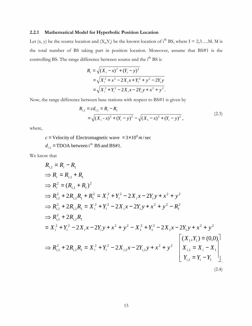
2.2.1 Mathematical Model for Hyperbolic Position Location

Let (x, y) be the source location and (Xi,Yi) be the known location of ith BS, where I = 2,3�.M. M is

the total number of BS taking part in position location. Moreover, assume that BS#1 is the

controlling BS. The range difference between source and the ith BS is

.22

22

)()(

2222

2222

22

yxyYxXYX

yYyYxXxX

yYxXR

iiii

iiii

iii

++−−+=

−++−+=

−+−=

Now, the range difference between base stations with respect to BS#1 is given by

,)()()()-( 221

22

11,1,

yYxXyYxX

RRcdR

iii

iii

−+−−−+=

−== (2.3)

where,

BS#1. and BSibetween TDOA sec/103 waveneticElectromag ofVelocity

th1,

8

dm c

i =

×==

We know that

−=−=

=++−−+=+⇒

++−−+−++−−+=

+⇒

−++−−+=+⇒

++−−+=++⇒

+=⇒

+=⇒

−=

11,

11,

1122

1,1,22

11,21,

2211

21

21

2222

11,21,

21

222211,

21,

22222111,

21,

211,

2

11,

11,

)0,0(),(222

2222

2

222

222

)(

YYYXXX

YXyxyYxXYXRRR

yxyYxXYXyxyYxXYX

RRR

RyxyYxXYXRRR

yxyYxXYXRRRR

RRR

RRRRRR

ii

iiiiiiii

iiii

ii

iiiiii

iiiiii

ii

ii

ii

.

(2.4)

16

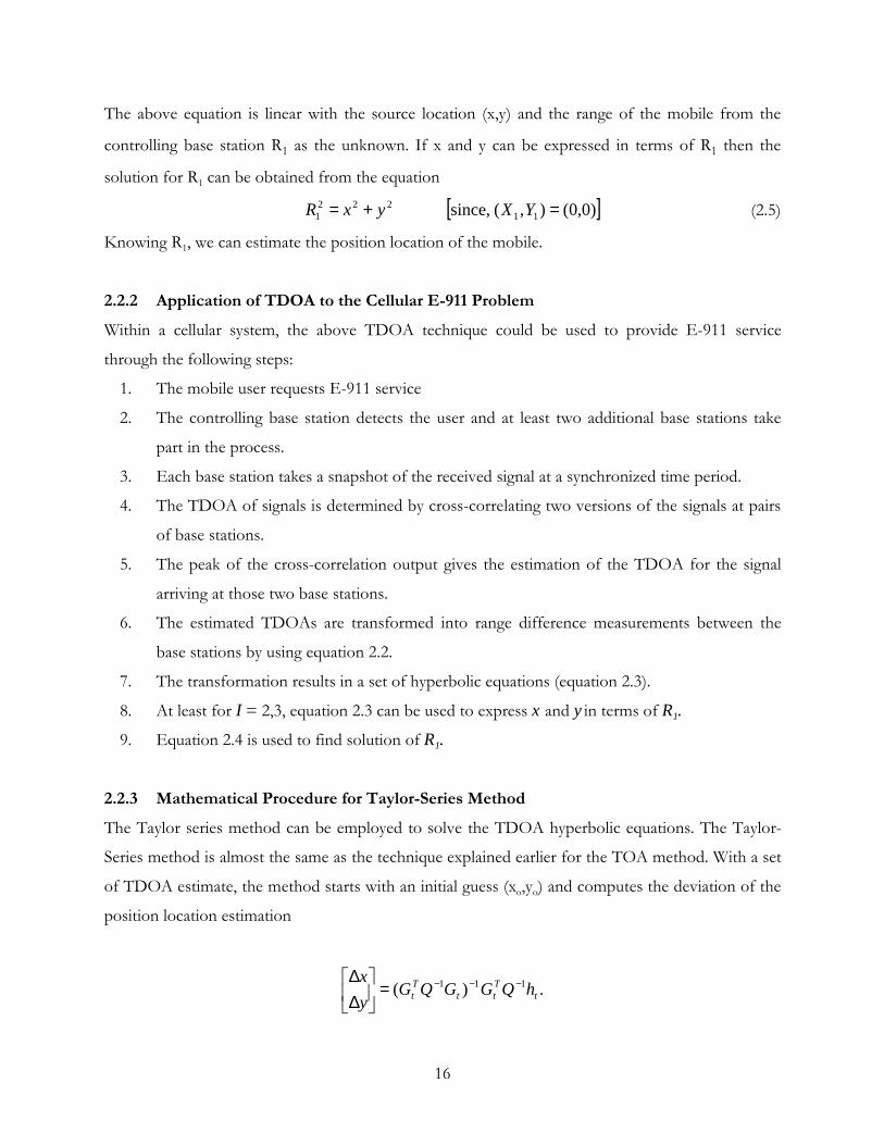
The above equation is linear with the source location (x,y) and the range of the mobile from the

controlling base station R1 as the unknown. If x and y can be expressed in terms of R1 then the

solution for R1 can be obtained from the equation

[ ] )0,0(),(,since 11222

1 =+= YXyxR (2.5)

Knowing R1, we can estimate the position location of the mobile.

2.2.2 Application of TDOA to the Cellular E-911 Problem Within a cellular system, the above TDOA technique could be used to provide E-911 service

through the following steps:

1. The mobile user requests E-911 service

2. The controlling base station detects the user and at least two additional base stations take

part in the process.

3. Each base station takes a snapshot of the received signal at a synchronized time period.

4. The TDOA of signals is determined by cross-correlating two versions of the signals at pairs

of base stations.

5. The peak of the cross-correlation output gives the estimation of the TDOA for the signal

arriving at those two base stations.

6. The estimated TDOAs are transformed into range difference measurements between the

base stations by using equation 2.2.

7. The transformation results in a set of hyperbolic equations (equation 2.3).

8. At least for I = 2,3, equation 2.3 can be used to express x and y in terms of R1.

9. Equation 2.4 is used to find solution of R1.

2.2.3 Mathematical Procedure for Taylor-Series Method The Taylor series method can be employed to solve the TDOA hyperbolic equations. The Taylor-

Series method is almost the same as the technique explained earlier for the TOA method. With a set

of TDOA estimate, the method starts with an initial guess (xo,yo) and computes the deviation of the

position location estimation

.)( 111t

Ttt

Tt hQGGQG

yx −−−=

∆∆

17

where,

.

1

1

1

1

3

3

1

1

3

3

1

1

2

2

1

1

2

2

1

1

,11,

131,3

121,2

and,

)(

)()(

−−−−−−

−−−−−−

−−−−−−

=

−−

−−−−

=

M

M

M

M

t

MM

t

RxY

RxY

RxX

RxX

RxY

RxY

RxX

RxX

RxY

RxY

RxX

RxX

G

RRR

RRRRRR

h

M

M

M

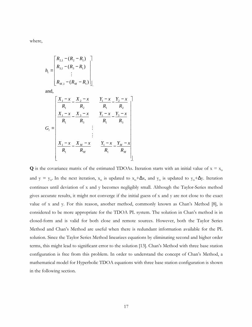
Q is the covariance matrix of the estimated TDOAs. Iteration starts with an initial value of x = xo

and y = yo. In the next iteration, xo is updated to xo+∆x, and yo is updated to yo+∆y. Iteration

continues until deviation of x and y becomes negligibly small. Although the Taylor-Series method

gives accurate results, it might not converge if the initial guess of x and y are not close to the exact

value of x and y. For this reason, another method, commonly known as Chan�s Method [8], is

considered to be more appropriate for the TDOA PL system. The solution in Chan�s method is in

closed-form and is valid for both close and remote sources. However, both the Taylor Series

Method and Chan�s Method are useful when there is redundant information available for the PL

solution. Since the Taylor Series Method linearizes equations by eliminating second and higher order

terms, this might lead to significant error to the solution [13]. Chan�s Method with three base station

configuration is free from this problem. In order to understand the concept of Chan�s Method, a

mathematical model for Hyperbolic TDOA equations with three base station configuration is shown

in the following section.

18

2.2.4 Mathematical Model for TDOA Equations in Chan�s Method For a three base station system, Chan�s method producing two TDOAs to render solution for x and

y in terms of R1 is of the form

,132

1,3

122

1,21

1,3

1,21

1,31,3

1,21,2

21

+−

+−+

×

−=

−

KKR

KKRR

RR

YXYX

yx

where,

.,

,

,,

1,31,3

1,21,2

23

233

22

222

21

211

cdRcdR

YXKYXKYXK

==

+=

+=

+=

In the above equation on the right side, all the quantities are known quantities except R1.

Therefore solution of x and y will be in terms of R1. When these values of x and y are substituted

into the equation, 2221 yxR += , a quadratic equation in terms of R1 is produced. Once the

roots of R1 are known, values of x and y can be determined. It should be noted that only the

positive root of R1 must be considered. One of the roots of the quadratic equation is either

negative or too large to be within the cell radius.

2.3 Measure of PL Estimator Performance Position estimator performance can be measured by several parameters, namely:

• Circular Error Probability (CEP)

• Geometric Dilution of Precision (GDOP)

• Mean Square Error (MSE)

• Cramer-Rao Lower Bound (CRLB)

CEP is based on the variances of the position estimate in the x direction and y direction. This gives

an overall measure of the position estimator accuracy. GDOP is a measure of the estimator�s

performance depending on the actual position of the mobile relative to the base stations. Every

position estimator performance can be evaluated by comparing estimator�s MSE to the Cramer-Rao

19

Lower Bound (CRLB). CRLB is the theoretical limit for the variance of the estimator�s output. We

briefly consider the definition and value of each of these performance measures.

2.3.1 Circular Error Probability (CEP) If an estimator is unbiased, CEP describes the scattering of the position estimate around the true

position of the MS. CEP is defined as the radius of a circle around the estimator�s position bias that

contains half of the generated estimates [5], as illustrated in figure 2.4.

CEP, within an accuracy of 10%, is given by [3] as:

,75.0 22yxCEP σσ +≅

where,

y x

y

x

ˆestimateposition of Variance

ˆestimateposition of Variance2

2

=

=

σσ

2.3.2 Geometric Dilution of Precision (GDOP) GDOP is the standard deviation of the range measurements [6]. Mathematically, it is defined as the

ratio of the RMS position error to the RMS ranging error, that is:

Figure 2.4: Circle of Error Probability

CEP

Real Mobile Position

Bias Vector

20

.75.0

22

s

s

yx

CEP

GDOP

σ

σσσ

≅

+=

From the above equation, it is evident that the GDOP is directly proportional to CEP, which means

that if the scattering of the position estimate around the true position of the MS is small the

estimator�s output variance will be small as well. The smaller the Root Mean Square (RMS) position

estimate error, the better the performance of the estimator.

2.3.3 Mean Square Error (MSE) MSE is the square of the distance between a true mobile-position and an estimated mobile-position.

Mathematically it is defined as,

,

,)ˆ()ˆ( 22

MSERMS

yyxxMSE

=

−+−=

where, x and y are the mobile�s real position. For most of the results in chapter 5 and 6, we will use

RMS error as the performance measure of interest.

2.3.4 Cramer-Rao Lower Bound In order to measure the accuracy of the position estimate, RMS position error of the estimator can

be compared to the theoretical limit for unbiased estimators. Chan [8] derived the CRLB as,

,)( 112 −−=Φ tt GQGc

where,

Gt = Taylor coefficients matrix evaluated at an initial guess (xo, yo),

Q = Covariance matrix of the smoothed and corrected range measurements that serve as

estimator input data,

c = Velocity of electro-magnetic wave in free space.

The theoretical limit for the RMS position error of the estimator is given by,

)(Φ= traceRMSLimit .

21

2.4 Chapter Summary In this chapter we have presented a discussion of range-based measurement techniques. The TOA

and TDOA techniques that will be used in the remainder of this thesis have been rigorously defined.

The chapter has also presented a discussion of performance measures for TOA and TDOA

techniques.

22

Chapter 3

Data Fusion

Data fusion means to combine the data obtained from different sensors, and relate information by

accessing relevant databases, to achieve better accuracies and more specific inferences than could be

found by the use of a single sensor alone [14]. The advent of sophisticated sensors, advanced

processing techniques, and fast processing hardware are making implementation of data fusion

practically a feasible option.

It is intuitive that when a same-source data is gathered by using multiple independent

sensors, this data should result in a statistical gain over a single source data. In data fusion

architecture, decision or inferences are made at different hierarchical levels. Identifying

characteristics of an entity and its location are the basis of the decision or inference process.

Therefore, hierarchical transformation between observed data and a corresponding decision or

inference is the basic characteristic of data fusion technology.

Data fusion is widely used both in military application and civilian application. Position and velocity

determination for a moving object from noisy time-series measurements is a classical statistical

estimation problem [15], [16], [17]. Classic detection and estimation methods are typically used for

raw data fusion techniques.

In the recent years data fusion technology has rapidly advanced from a loose collection of

related techniques to an emerging engineering discipline with standard terminology [14]. Lack of

unifying terminology impeded the technology transfer from one group to another in this field. In

order to improve communications among military and civilian researchers and system developers,

the Joint Director of Laboratories (JDL) established a data-fusion working group that devised

generic data fusion architecture in 1972 [5].

3.1 JDL Data Fusion Architecture The JDL data fusion architecture is a conceptual model. It identifies and categorizes the process,

functions, and techniques applicable to data fusion. When developed, the JDL process model was

intended to be very general and useful for multiple applications in different areas. For this reason it

23

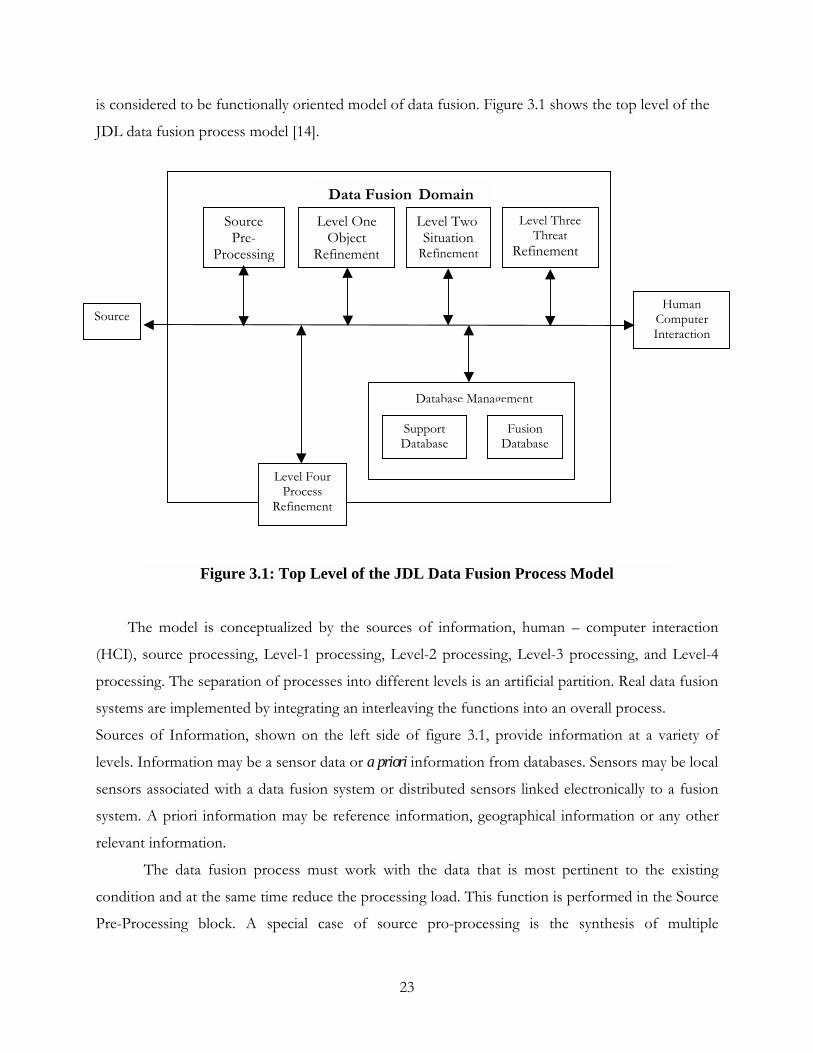
is considered to be functionally oriented model of data fusion. Figure 3.1 shows the top level of the

JDL data fusion process model [14].

The model is conceptualized by the sources of information, human � computer interaction

(HCI), source processing, Level-1 processing, Level-2 processing, Level-3 processing, and Level-4

processing. The separation of processes into different levels is an artificial partition. Real data fusion

systems are implemented by integrating an interleaving the functions into an overall process.

Sources of Information, shown on the left side of figure 3.1, provide information at a variety of

levels. Information may be a sensor data or a priori information from databases. Sensors may be local

sensors associated with a data fusion system or distributed sensors linked electronically to a fusion

system. A priori information may be reference information, geographical information or any other

relevant information.

The data fusion process must work with the data that is most pertinent to the existing

condition and at the same time reduce the processing load. This function is performed in the Source

Pre-Processing block. A special case of source pro-processing is the synthesis of multiple

Figure 3.1: Top Level of the JDL Data Fusion Process Model

Source

Source Pre-

Processing

Level One Object

Refinement

Level TwoSituation

Refinement

Level Three Threat

Refinement

Human Computer Interaction

Database Management

SupportDatabase

FusionDatabase

Level Four Process

Refinement

Data Fusion Domain

24

component sensory array data to estimate the location and the velocity of a target [14]. In order to

successfully accomplish this, all the data must be prescreened and allocated to an appropriate

process.

Level-1 operates on raw data and performs multiple functions. It first transforms data to a

consistent set of units and coordinates, then estimates the object�s attribute, and refines prediction

based on statistical estimation. In short, level-1 processing is responsible for combining locational,

parametric and identity information to achieve refined representations of individual objects [14].

Level-2 does situation refinement focusing on relational information so as to determine the

meaning of a number of separately collected entities. This level attempts to improve a description of

current relationships among objects and events in the context of their environment [5].

Level-3 uses Fast-Time Engagement Models to aggregate estimation so as to predict the

projection of current situation in future based on multi perspective assessment. If necessary, level-3

deduces alternative hypothesis from input data of the process.

Level-4 acts as a watchdog to other processes. It is also termed as meta-process, meaning that

the process is concerned about other processes. It monitors the data fusion performance and

identifying information to improve multi-level data fusion output.

Data base management acts as the heart of the JDL DF model. It performs data retrieval and

storage, archiving, queries, and data protection so that it can support the entire process at all the

levels.

HCI incorporates multimedia methods for human interaction. Communication of fusion

system results may be through different types of media, like display via monitors, notification by

alert or printing in text using printers.

The JDL DF model is helpful for common understanding, but does not help in developing

architecture for real system [18]. Hall [14] proposed a hybrid approach that combines level one and

level two fusion based on the JDL model.

3.2 Data Fusion Model for Position Location Estimation Section 3.1 discussed the general JDL DF model, which is helpful in understanding the basic

concept of DF process. Since the JDL DF model is a functionally oriented model, therefore to make

this model applicable to position location problem, Kleine-Ostmann and Bell [23] have proposed an

architecture using first, second, and fourth level fusion. Figure 3.2 shows the model proposed by

Kleine-Ostmann and Bell.

25

The main objective behind this technique is to fuse both TOA and TDOA data, obtained

independently, in order to have an estimate better than either of the individual estimates. It should

be noted that, in the proposed architecture, fusion is done with raw TOA/TDOA data as well as

final position estimation generated by two different methods. It is important to mention that two

different methods have two different error biases and variances. Therefore, care should be taken to

weight TOA and TDOA measurement according to their quality, at least in terms of their variances.

The proposed structure estimates position of the E-911 mobile user by four different approaches

before making a final choice. First estimation is done only from TOA measurements using the

algorithm described in Section 2.1. Then estimation is made only from TDOA measurements using

Figure 3.2: Proposed Data Fusion Model for Position Estimation

TOA Measurements

(Corrected)

TDOA Measurements

(Corrected)

TOA

Position Estimator

TS-LS Method

TDOA

Position Estimator

TS-LS Method

Second Level Data Fusion Process

Level Four Data Fusion Process

Best Choice of Position Estimation

Optimal

Position Estimate

Converted TDOA

First Level Data Fusion

Position Estimator

26

the algorithm described in the Section 2.2. Combining the raw TOA and TDOA data makes

estimation from the first level data fusion. According to the data fusion standard, only a similar kind

of data can be fused. Therefore, the TOA data must be converted to the corresponding TDOA data

before fusing at the first level. This is accomplished by simply subtracting one set of TOA

measurements from another set. The fourth position estimation is done at second level hierarchy. At

this level Bayesian Inference is used to produce new improved estimate while combining the two

position estimates form the TOA estimator and TDOA estimator. All these four estimates are then

fed into level-4 processor, which decides which one of the four position estimates offers the best

accuracy.

3.2.1 First Level Data Fusion At the first level data fusion process, independent TOA measurements are converted to the

corresponding TDOA measurements. These converted measurements are then combined with the

independent TDOA measurements. Since the system we are considering generate an over-

determined system of equations, therefore weighted least-square (WLS) estimator is employed to

minimize the sum of the weighted squares of the errors. This kind of estimator is implemented for

independent TDOA estimator described in the Chapter 2. The only difference is that the matrix Gt

is augmented with additional rows for TDOA measurements resulting from independent TOA

measurements. Now the new solution is obtained from more measurements.

3.2.2 Second Level Data Fusion The second level data fusion utilizes the Bayesian Inference to improve an estimate with known

statistics once new data is available [26]. If xo and σ2o are the mean and variance respectively of the

TOA estimator output, and xm and σ2m are the mean and variance respectively of the TDOA

estimator output, then xc would be the mean and σ2c would be the variance of a single estimate

using the Bayesian Inference. The probability distribution of the old estimate is updated depending

on the probability distribution of new data and the amount of data available. Figure 3.3 shows the

principle of the Bayesian Inference. In Figure 3.3 the center of mass xc serves as an improved

estimate over xo and xm, and the variance of new distribution indicates the weight of reliability of the

improved estimate.

27

Figure 3.3: Bayesian Inference Since both TOA and TDOA measurements are assumed to have Gaussian distribution [19], the

center of mass of new distribution or, in other words, the fused position estimate becomes,

( )ommo

oo

mo

m

m

o

o

c xxx

xx

x −+

+=+

+

=22

2

22

22

11 σσσ

σσ

σσ

the variance σ2c is given by,

22

211

1

mo

c

σσ

σ+

=

Simulation results using this proposed architecture is presented in the following chapter.

3.2.3 Level Four Data Fusion: The final choice Level four is the process where decision is made, which one of the all estimates represents the best

choice. Solely evaluating the variance of each estimator output makes this decision. The second level

estimate is expected to show reduced variance and hence be more reliable. Although the TDOA

xo xc xm

new sample

a posterior distribution

a priori distribution

Position estimate

P

28

estimator has an inherent characteristic to be more tolerant to error bias introduced due to NLOS

between BS and MS, it performs poorly when MS is very close to the BS.

3.3 Chapter Summary In this chapter we have summarized the basic concepts of data fusion that will be used in chapters 5

and 6 of this thesis to combine TOA and TDOA estimates of mobile position within an E-911

system. This chapter outlined the different levels of data fusion that are available for combining data

from disparate sources.

29

Chapter 4

The Channel Models

The effects of the mobile radio channel dominate the performance of a wireless communication

system. The path along which a signal travels between a transmitter and a receiver could be either a

simple line-of-sight one or a highly obstructed one. High rise buildings, mountains, or vegetation

causes this obstruction along the path. Therefore, modeling the radio channel has been one of the

most challenging parts of mobile radio system design. Often this modeling follows a statistical

approach [20]. This chapter develops the channel models employed in chapters 5 and 6 to evaluate

data fusion techniques for combining TOA and TDOA position estimates. The effects considered

in this model include the path loss, result of AWGN and multi-path channels, as well as generation

of received signals at the base stations.

Received Signal Models 4.1.1 TOA Received Signal Model The range measurements between the base station and the mobile unit are linearly proportional to

the TOA measurements. Although electromagnetic waves pass through different kind of medium

while traveling along the path from a transmitter to a receiver, their speed can be considered

constant, as the obstructed path length is much smaller than the traveling path in the air. Figure 4.1

illustrates this concept. When there is a complete LOS between the base station and the mobile unit,

only the standard measurement noise affects the true range measurements. This standard

measurement noise is assumed to have a distribution, which is similar to Gaussian distribution but

with fine support region. However, in our simulation we have simulated the standard noise by a zero

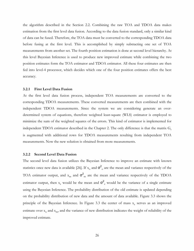
mean Gaussian random variable. Figure 4.2 shows the probability distribution function of standard

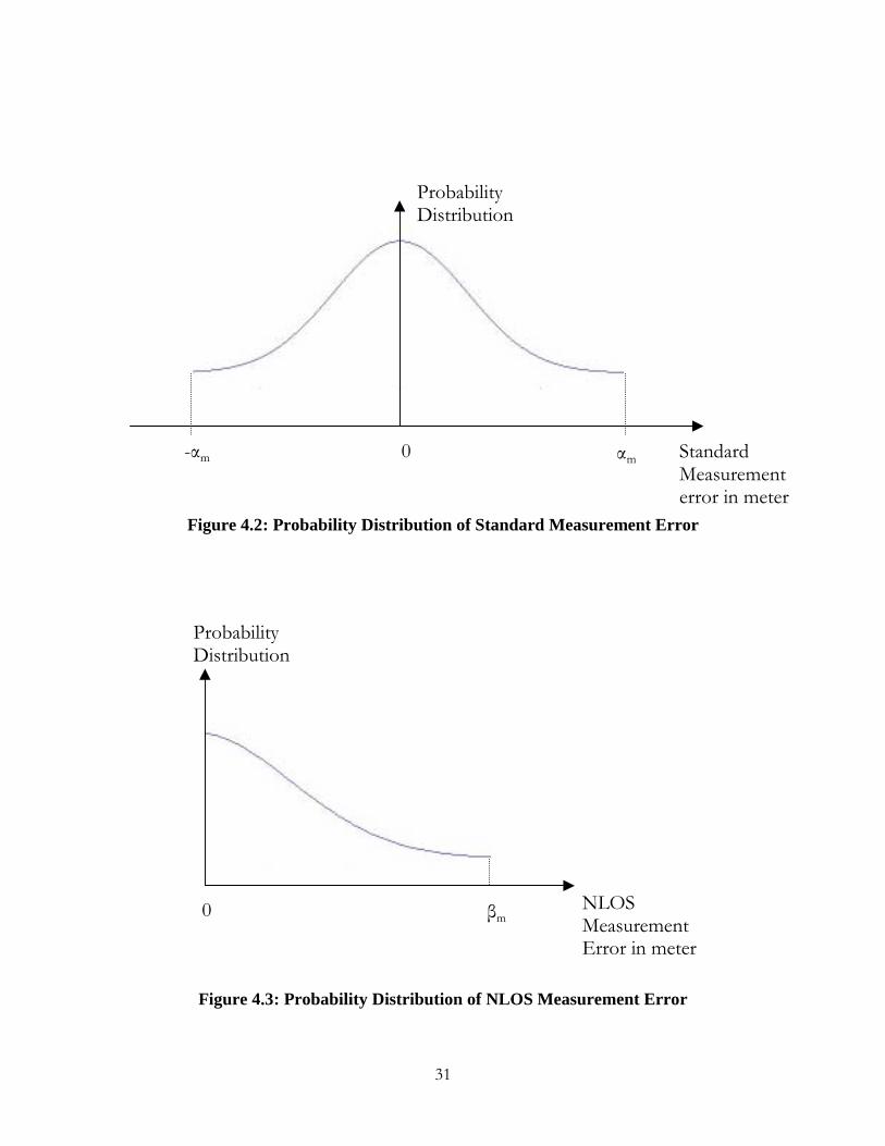
measurement noise. In case when there is NLOS between the base station and the mobile unit, the

measured ranges would be biased and the variance would be higher than the one obtained in LOS

case. This appears to be an additional noise in the measured ranges. The empirical measurements

have shown that NLOS error has a distribution like the one shown in Figure 4.3, which appears to

be a single sided Gaussian distribution with bounded region. Therefore, the range measurements of

TOA PL system is modeled as in equation 2.1:

30

)()()()( imimimimTOA tNLOStntLtrr ++== ,

where,

( ) ( )

( ) ( ) mi

m

mimmm

m

t

NLOS

tnn

L

K

Ki

m

βσµ

αασ

≤≤≈

=

≤≤−≈=

=

=

−==

==

mNLOS

m

i

NLOS 0 ,N

sight,-of-line-Non todueError

,0,Nerrort measuremen Standard

, BS and MSbetween distance True

, ttimedifferent at tsmeasuremen ofNumber

),1.....(2,1,0index timeSample

M,....2,1index BS

Figure 4.1: Propagation of EM Waves through different Medium

Rx

Tx Traveling distance through a medium

EM Wave

Obstructingmedium

31

Figure 4.2: Probability Distribution of Standard Measurement Error

Figure 4.3: Probability Distribution of NLOS Measurement Error

Standard Measurement error in meter

αm -αm

ProbabilityDistribution

0

βm

ProbabilityDistribution

NLOSMeasurement Error in meter

0

32

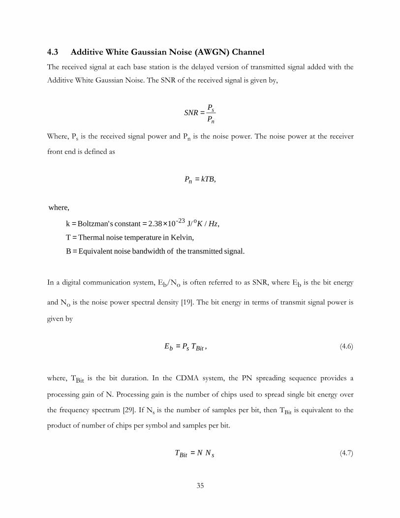
4.1.2 TDOA Received Signal Model The received signals at the base stations are the delayed versions of the transmitted signal from the

mobile unit with noise superimposed on the signals. Assuming a four base station configuration,

with base station #1 as the controlling base station, then for the propagation delays d1, d2, d3, and d4

at base stations 1, 2, 3 and 4 respectively, the relative delays with respect to the controlling base

station are given by,

.

,

,

1441

1331

1221

ddd

ddd

ddd

−=

−=

−=

Each base station generates a particular sequence of BPSK signal, which is sampled and shifted

accordingly to the relative delays. Delays are determined based on the distance of the mobile from

each of the participating base stations. The signal passed through the Additive White Gaussian

Noise (AWGN) channel, where noise power is scaled according to the Signal-to-Noise Ratio (SNR)

of the received signal.

The general model for the received signals at different base stations are given by,

( ) ( ) ( )( ) ( ) ( )( ) ( ) ( )( ) ( ) ( ) ,

,

,

,

44144

33133

22122

11111

tndtsAtr

tndtsAtr

tndtsAtr

tndtsAtr

+−=

+−=

+−=

+−=

(4.1)

where Ai [ i = 1, 2, 3, 4 ] is the amplitude scaling of the signal and ni(t) [ i = 1, 2, 3, 4] is the noise

and the interfering signals. Since BS#1 is the controlling base station, therefore d1 < di [ i = 2, 3, 4].

If the delay time and the scaling amplitudes are referred to the controlling base station, then the

received signals at the neighboring base stations would be time shifted versions of the received

signal at the controlling BS#1. The models of equation 4.1 can be rewritten as:

33

( ) ( ) ( )( ) ( ) ( )( ) ( ) ( )( ) ( ) ( ).

,

,

,

44114

33113

22112

111

tndtstr

tndtstr

tndtstr

tntstr

+−=

+−=

+−=

+=

(4.2)

Since a log-distance path loss model is used, therefore each received signal power levels are adjusted

depending on the channel path loss exponent and distance from the mobile unit to the base station.

The TDOA estimator then processes the received signals where the hyperbolic location algorithm is

used to provide an estimate of the mobile�s position location. Figure 4.4 [21] shows the block

diagram of the simulator used for generating TDOA signals and determining position estimate of

the mobile unit.

Figure 4.4: Block Diagram of TDOA Simulator

Establish Mobile Position

Determine Range

from BS#i ii R

cd = Delaysd1, d2 , d3

Generate Signal

n1(t)

d3

n3(t)

n2(t)

Peak Correlation Detector

PeakCorrelation Detector

Taylor Series Algorithm

Estimated Mobile Position

TDOA Estimate #1 TDOA Estimate # 2

d1 d2

34

4.2 Path Loss Model The log-distance path loss model has been developed based on theoretical analysis as well as

practical measurements. The model indicates the average received signal power that decreases

logarithmically with distance. If d0 is the close-in reference distance and n is the path loss exponent,

then the average large-scale path loss for an arbitrary transmitter-receiver separation distance d is

given by:

[20]. log10)()(0

0

+=

ddndPLdBPL (4.3)

In order to avoid near-field effects, the close-in reference distance must be chosen in such a way that

it lie in the Fraunhofer region. The near-field effects otherwise may alter the reference path loss. The

dimension of the transmitting antenna and the operating frequency defines the far-field distance.

The far-field distance is given by

,2 2

λD

d f = (4.4)

where, D is the maximum dimension of the transmitting antenna and λ is the wavelength at the

operating frequency. With PCS carrier frequency of 1900 MHz, and half-wave dipole antenna, the

Fraunhofer distance is 0.08 meter. For our simulation, 100 meter is the close-in reference distance

for macro-cellular environment. If PtGt is the EIRP of mobile unit transmitter, then the power at a

distance d0 is given by

,4

log20dBm)( 00

−++=λ

πdGGPdP rttr (4.5)

where, Gr is the receiving antenna gain and λ is the wavelength at the operating frequency. The

signal power received in a base station, located at a distance d from the mobile unit is given by,

.log10dBm)(dBm)(0

0

−=

ddndPdP rr

35

4.3 Additive White Gaussian Noise (AWGN) Channel The received signal at each base station is the delayed version of transmitted signal added with the

Additive White Gaussian Noise. The SNR of the received signal is given by,

n

sPP

SNR =

Where, Ps is the received signal power and Pn is the noise power. The noise power at the receiver

front end is defined as

,kTBPn =

signal. ed transmitt theofbandwidth noise Equivalent B

Kelvin,in re temperatunoise Thermal T

,/J/ 10 2.38 constant sBoltzman' k

,whereo23-

=

=

×== HzK

In a digital communication system, Eb/No is often referred to as SNR, where Eb is the bit energy

and No is the noise power spectral density [19]. The bit energy in terms of transmit signal power is

given by

,Bitsb TPE = (4.6)

where, TBit is the bit duration. In the CDMA system, the PN spreading sequence provides a

processing gain of N. Processing gain is the number of chips used to spread single bit energy over

the frequency spectrum [29]. If Ns is the number of samples per bit, then TBit is equivalent to the

product of number of chips per symbol and samples per bit.

sBit NNT = (4.7)

36

For AWGN channel, the noise power is given by,

20

02

22

n

n

N

N

σ

σ

=⇒

= (4.8)

From equation (4.6), (4.7) and (4.8)

.2

,22

0

2

220

=⇒

==

NE

NNP

NNPTPNE

b

ssn

n

ss

n

Bitsb

σ

σσ

(4.9)

Since unity power signal is used for simulation, therefore Ps = 1 and noise power for a given SNR is

obtained from

.2

0

2

=

NENN

b

snσ (4.10)

A zero mean Gaussian noise with a variance given by equation (4.10) is added to the delayed version

of transmitted signal from the mobile unit to represent received signals at the corresponding base

stations.

4.4 Chapter Summary This chapter has summarized channel models employed to simulate wireless propagation effects

within a cellular environments. These channel models are employed in Chapter 5 to evaluate data

fusion of TOA and TDOA position estimates and then again in Chapter 6 to evaluate data fusion

with TDOA estimates corrected for the LOS cases.

37

Chapter 5

Data Fusion With Uncorrected TDOA

This chapter presents partial simulation results related to the PL solution for data fusion with

uncorrected TDOA. In Chapter 6, we consider the extension of these results to the case where

TDOA measurements are corrected for NLOS propagation. Some assumptions are made regarding

the mobile user position as well the CDMA system while developing the PL simulator. The E-911

user is assumed to be stationary in all simulation cases. This reflects the physical scenario where a car

may be broken on a highway, and the driver may be asking for the service while seating inside or

standing beside the car. The sections 5.2 and 5.3 present simulation results that validate the

performance of the TOA and TDOA simulator. Finally, the performance of the data fusion

simulator with corrected TOA and uncorrected TDOA measurements is discussed.

5.1 Simulation Models The base stations configuration used for all simulations is shown in figure 5.1. There are four

participating base stations, and three of them are uniformly spaced around a circle and the other one

is located at the center of the circle.

Figure 5.1: Base Stations Configuration

y

x

BS #4

(0, 5000)

BS #2

(4330, -2500) BS #3

(-4330, -2500)

BS #1(0, 0)

R = 5000

MS (x, y)

38

Base station #1 is assumed to be the controlling base station, meaning that the mobile user is within

the cell where the BS#1 is the serving base station. It is also assumed that the controlling base

station will always be at the center of the coordinate system. Since it is assumed that the system is

operating in the CDMA environment, the mobile unit transmitter is modeled as the one shown in

Figure 5.2. In an ealier chapter we mentioned that, a half-wave dipole antenna with unity gain and

maximum transmiiter power of 1 Watt will be used in all simulations. The carrier frequency of 1900

MHz, and a chip rate of 1.2288 Mcps are used which indicate the operation of the CDMA system in

the PCS band. One important thing is worth mentioning that, a perfect RF modulation and

demodulation is assumed throughout this research work. 1.2288 Mcps chip rate indicates the

modulating signal bandwidth to be 1.2288 MHz. A Non-Return to Zero (NRZ) waveform with unit

amplitude are assumed for both PN spread sequence and message signal. It is well known that,

sampling plays an important role in digital communication. In order to have sufficient Signal-to-

Aliasing Ratio (SAR), an over sampling rate of 10 samples/symbol is used in all simulations. Figure

5.3 shows a plot of SAR vs Sample-per-Symbol. Since base band binary system operate with a true

SNR of the order of 10 dB, sampling rate must be such that the SAR is much greater than 10 dB.

This is to ensure that aliasing error does not affect the simulated performance of the system [22].

From figure 5.3 we find that, SAR is close to 17 dB for sampling rate of 10 samples per symbol. For

all simulations over sampling rate of 10 samples/symbol is used. In CDMA One cellular standard,

the long PN spreading sequence introduces a processing gain of 4 per symbol after rate 1/3

convolutional encoder. A 64-ary orthogonal modulator introduces an additional processing gain of

32 per symbol. Therefore, the over all processing gain in CDMA One cellular standard is 128. In all

our simulations, we have assumed a constant processing gain of 128. Closed-loop power control is

also assumed for every simulation. This indicates that, the total power level of each user on the

receiving antenna of the primary base station is equal, thereby eliminating any near-far problem

encountered in CDMA system. It is assumed that, unless specified, the controlling base station has

to maintain a Signal-to-Noise Ratio of 10 dB from all users within the cell.

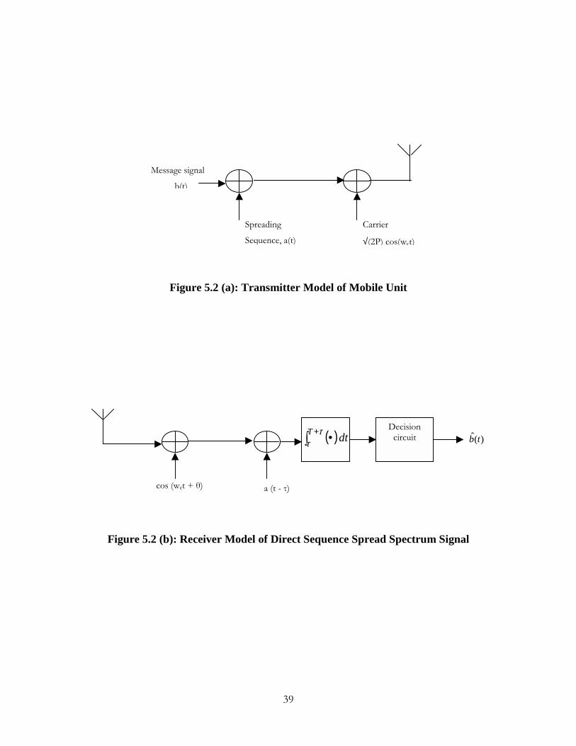
39

Figure 5.2 (a): Transmitter Model of Mobile Unit

Figure 5.2 (b): Receiver Model of Direct Sequence Spread Spectrum Signal

Message signal

b(t)

Spreading

Sequence, a(t)

Carrier

√(2P) cos(wct)

( )dtT∫

+ •ττ

Decision circuit )(ˆ tb

cos (wct + θ) a (t - τ)

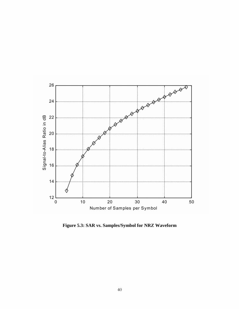
40

0 10 20 30 40 5012

14

16

18

20

22

24

26

Number of Samples per Symbol

Sig

nal-t

o-A

lias

Rat

io in

dB

Figure 5.3: SAR vs. Samples/Symbol for NRZ Waveform

41

5.2 Validation of TOA Simulator Performance The Wylie-Holtzman data model will be used to synthesize the TOA ranges. Once the true distance

between the mobile user and the base station is determined, the standard measurement noise and the

NLOS noise, where applicable, are added to the true range. In order to validate that the simulator is

working properly, mobile trajectory estimation test is performed. The simulator makes necessary

measurements to determine NLOS case and then takes appropriate steps to correct the errors

introduced due to non-line of sight between the mobile and the base station. The starting point of

the mobile trajectory is (300, 300) and velocity of the mobile is (vx = 9.7m/sec, vy = 16.8 m/sec).

The estimator would estimate mobile trajectory from a series of measurements taken at different

time. As we assumed earlier that the mobile requesting for E-911 service is stationary, it is not

always necessary to estimate the entire trajectory of the mobile user. Once we validate that the

simulator is working properly, the velocity of the mobile will be set to zero and the performance of

the Taylor-Series Least-Square estimator will be evaluated based on the mean and variance of the

position estimates obtained at different mobile locations.

5.2.1 Mobile Trajectory Estimation In this simulation we assume that the mobile is moving along a straight line. Therefore at any given

instant t, the mobile position is obtained from the equation 5.1.

( )( ) tvyty

tvxtx

yo

xo

+=+=

(5.1)

250 samples are taken at an interval of 0.5 second. The values used for the standard measurement

noise and NLOS noise are taken from the ones provided in the reference number 4. The standard

measurement noise is independent identically distributed Gaussian random variable with zero mean

and 150 meter standard deviation. The NLOS error is described as a positive sided Gaussian

random variable with 513 meters mean and 436 meter standard deviation. The values for αm and βm

are 400 meters and 1300 meters respectively. It is assumed that the BS#2 and the BS#4 always had

NLOS measurement while the BS#1 and the BS#3 always had complete LOS. Figure 5.5 shows the

plot of real mobile trajectory and the estimated mobile trajectory.

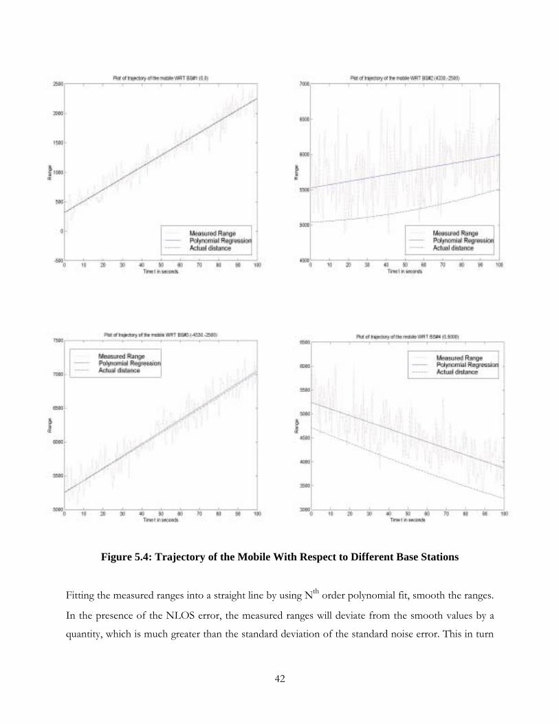
42

Figure 5.4: Trajectory of the Mobile With Respect to Different Base Stations

Fitting the measured ranges into a straight line by using Nth order polynomial fit, smooth the ranges.

In the presence of the NLOS error, the measured ranges will deviate from the smooth values by a

quantity, which is much greater than the standard deviation of the standard noise error. This in turn

43

means that the standard deviation of the measured ranges in case of an NLOS would be much

greater than the standard deviation of range measurements in case of an LOS. This hypothesis is

used to determine the base station having an NLOS. The threshold value for comparing the

standard deviation of the measured ranges from the smooth values is taken to be 300 meter. Table

5.1 and 5.2 show results that validate that it is possible to identify the NLOS measurements using

the hypothesis test. Table 5.2 shows results demonstrating the situation that all the four base stations

have NLOS.

Table 5.1: Standard Deviation of TOA Measurements from Smoothed Curves

Table 5.2: Standard Deviation of TOA Measurements from Smoothed Curves

BS# NLOS mσ

1 Yes 369.4

2 Yes 345.5

3 Yes 377.2

4 Yes 388.8

From Table 5.1 it is evident that the BS#2 and the BS#4 are identified to have an NLOS. Once an

NLOS is identified to exist for these two base stations, the Wylie-Holtzman algorithm is used to

eliminate the bias in the data introduced by the NLOS error. Figure 5.5 shows plot of maximum and

minimum values of the standard measurement noise as a function of number of trials. 250 samples

in each trial are used to determine the maximum and minimum value of noise. This figure gives an

idea about the bound of the standard measurement noise used in this simulation. The mean value of

BS# NLOS mσ

1 No 146.3

2 Yes 380.8

3 No 133.74

4 Yes 343.7

44

the upper bound of the standard measurement noise is 422 meter. Therefore the smooth curves for

the base stations having an NLOS will be shifted by this value.

0 50 100 150 200 250 300 350 400 450 500350

400

450

500Plot of Upper Bound of Std. Noise for TOA

Number of Iterations

Ran

ge o

f Upp

er B

ound Mean at Iteration

Overall Mean

0 50 100 150 200 250 300 350 400 450 500-500

-450

-400

-350

-300Plot of Lower Bound of Std. Noise for TOA

Number of Iterations

Ran

ge o

f Low

er B

ound Mean at Iteration

Overall Mean

Figure 5.5: Upper and Lower Bound of Standard Measurement noise of TOA

ranges

In the Figure 5.4, the dotted lines are the measured ranges, the solid lines are the smoothed range

measurements and dash-dotted lines represent a true mobile trajectory. Figure 5.6 shows the output

of the Least-Square estimator for different kind of inputs. The solid line indicates the real mobile

trajectory. The dash-dotted line shows the output of an LS estimator with the uncorrected smoothed

range measurements fed as the input, and the dashed line represents the estimated trajectory when

the Wylie-Holtzman algorithm is applied to the uncorrected input the estimator input. In order to

compare the improvement obtained by the Wylie-Holtzman algorithm, mobile trajectory is

estimated when all the participating base stations have complete line of sight with the mobile. The

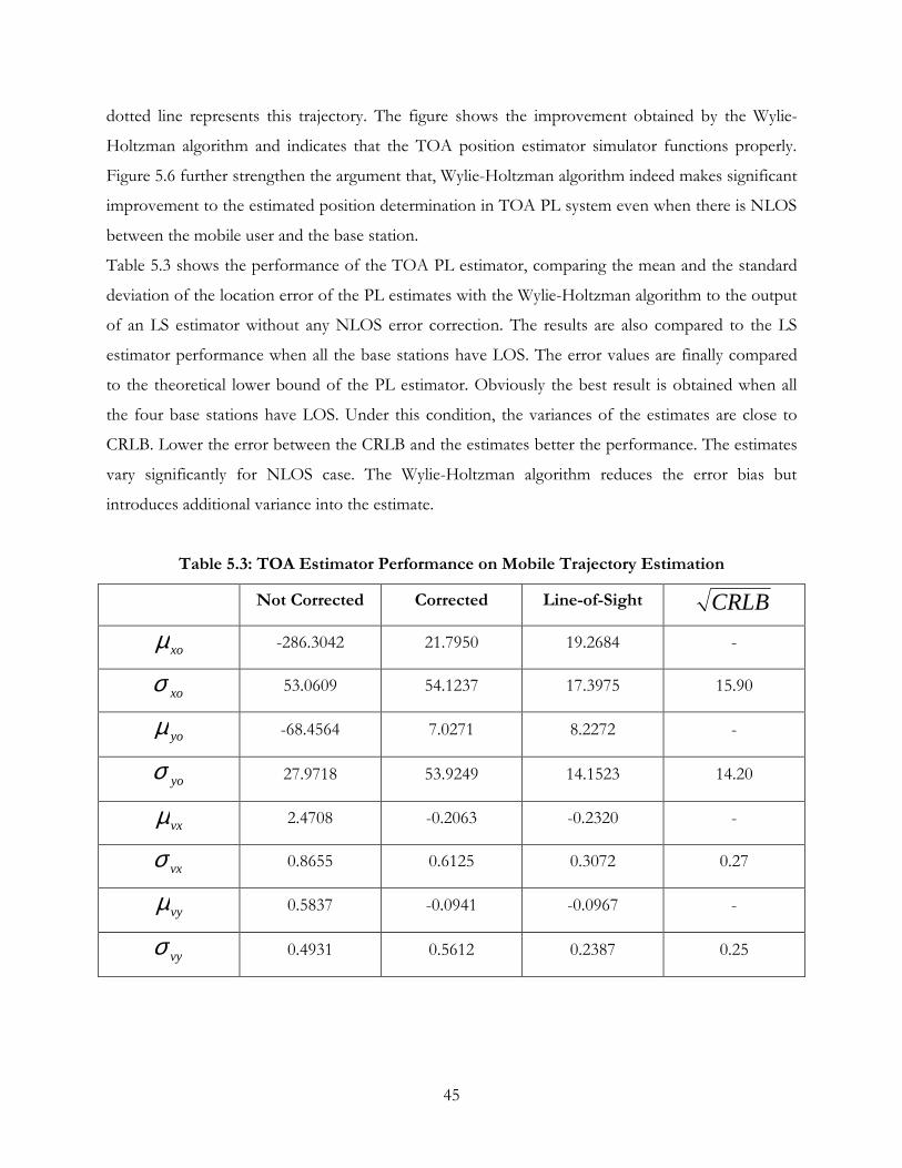
45

dotted line represents this trajectory. The figure shows the improvement obtained by the Wylie-

Holtzman algorithm and indicates that the TOA position estimator simulator functions properly.

Figure 5.6 further strengthen the argument that, Wylie-Holtzman algorithm indeed makes significant

improvement to the estimated position determination in TOA PL system even when there is NLOS

between the mobile user and the base station.

Table 5.3 shows the performance of the TOA PL estimator, comparing the mean and the standard

deviation of the location error of the PL estimates with the Wylie-Holtzman algorithm to the output

of an LS estimator without any NLOS error correction. The results are also compared to the LS

estimator performance when all the base stations have LOS. The error values are finally compared

to the theoretical lower bound of the PL estimator. Obviously the best result is obtained when all

the four base stations have LOS. Under this condition, the variances of the estimates are close to

CRLB. Lower the error between the CRLB and the estimates better the performance. The estimates

vary significantly for NLOS case. The Wylie-Holtzman algorithm reduces the error bias but

introduces additional variance into the estimate.

Table 5.3: TOA Estimator Performance on Mobile Trajectory Estimation

Not Corrected Corrected Line-of-Sight CRLB

xoµ -286.3042 21.7950 19.2684 -

xoσ 53.0609 54.1237 17.3975 15.90

yoµ -68.4564 7.0271 8.2272 -

yoσ 27.9718 53.9249 14.1523 14.20

vxµ 2.4708 -0.2063 -0.2320 -

vxσ 0.8655 0.6125 0.3072 0.27

vyµ 0.5837 -0.0941 -0.0967 -

vyσ 0.4931 0.5612 0.2387 0.25

46

Figure 5.6: Estimated Mobile Trajectory with and with out TOA Range

Correction

5.2.2 Evaluation of the Estimator�s Performance for Position Estimation In section 5.2 we mentioned that, for an E-911 service, it is not necessary to estimate the entire

trajectory of the mobile. Most applications of position estimators require determining only the

position estimates. In order to simulate this situation we set the velocity of the mobile to zero, and

calculate several position estimate mean and variance. This will give a chance to evaluate the

performance of an absolute position estimator.

Although the estimator is no longer estimating the mobile trajectory, the Wylie-Holtzman correction

algorithm still holds, and the smoothed curve and the corrected curve shown in figure 5.6 become

horizontal lines. The estimator directly outputs the estimate of the x-coordinate and the y-coordinate

of the mobile. These values are used to calculate the mean and variance of the estimates. Each

calculation uses 200 samples. Table 5.4 shows the estimated position location as well as the range

bias and the range standard deviation. CRLB is also included to compare the standard deviation to

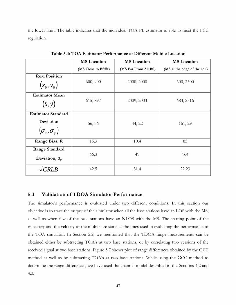
47

the lower limit. The table indicates that the individual TOA PL estimator is able to meet the FCC

regulation.

Table 5.4: TOA Estimator Performance at Different Mobile Location

MS Location

(MS Close to BS#1)

MS Location (MS Far From All BS)

MS Location (MS at the edge of the cell)

Real Position

( )00 , yx 600, 900 2000, 2000 600, 2500

Estimator Mean

( )yx ˆ,ˆ 615, 897 2009, 2003 683, 2516

Estimator Standard Deviation

( )yx σσ , 56, 36 44, 22 161, 29

Range Bias, R 15.3 10.4 85

Range Standard

Deviation, σr

66.3 49 164

CRLB 42.5 31.4 22.23

5.3 Validation of TDOA Simulator Performance The simulator�s performance is evaluated under two different conditions. In this section our

objective is to trace the output of the simulator when all the base stations have an LOS with the MS,

as well as when few of the base stations have an NLOS with the MS. The starting point of the

trajectory and the velocity of the mobile are same as the ones used in evaluating the performance of

the TOA simulator. In Section 2.2, we mentioned that the TDOA range measurements can be

obtained either by subtracting TOA�s at two base stations, or by correlating two versions of the

received signal at two base stations. Figure 5.7 shows plot of range differences obtained by the GCC

method as well as by subtracting TOA�s at two base stations. While using the GCC method to

determine the range differences, we have used the channel model described in the Sections 4.2 and

4.3.

48

10 15 20 25 300

0.2

0.4

0.6

0.8

1

SNR in dB

Nor

mal

ized

Ran

ge D

iffer

ence

GCC Output R21 TOA Derived R21GCC Output R31 TOA Derived R31GCC Output R41 TOA Derived R41

Figure 5.7: Normalized Range Differences vs. Signal-to-Noise Ratio

From Figure 5.7, we find that, at high SNR the TDOA range measurements from the cross

correlator output match with the values obtained from the models. In simulations, TDOA range

measurements obtained by using the GCC method take longer time than the measurements

obtained from the TOA measurements. Therefore subtracting the synthesized TOA range

measurements generates the TDOA range measurements in the simulations. In the next chapter we

will propose a data model that can be unswervingly used to synthesize TDOA range measurements.

Once again, when we validate that the simulator is working properly, the velocity of the mobile will

be set to zero and the performance of the Taylor-Series Lease Square estimator will be evaluated at

different mobile positions.

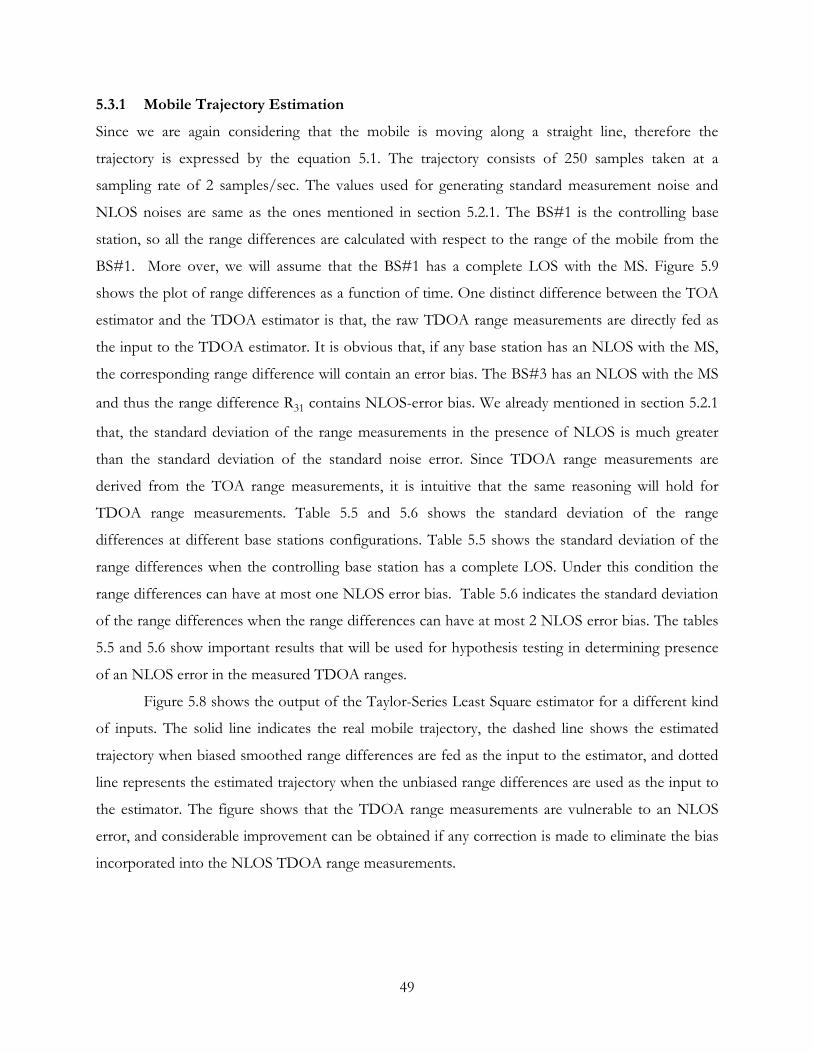
49

5.3.1 Mobile Trajectory Estimation Since we are again considering that the mobile is moving along a straight line, therefore the

trajectory is expressed by the equation 5.1. The trajectory consists of 250 samples taken at a

sampling rate of 2 samples/sec. The values used for generating standard measurement noise and

NLOS noises are same as the ones mentioned in section 5.2.1. The BS#1 is the controlling base

station, so all the range differences are calculated with respect to the range of the mobile from the

BS#1. More over, we will assume that the BS#1 has a complete LOS with the MS. Figure 5.9

shows the plot of range differences as a function of time. One distinct difference between the TOA

estimator and the TDOA estimator is that, the raw TDOA range measurements are directly fed as

the input to the TDOA estimator. It is obvious that, if any base station has an NLOS with the MS,

the corresponding range difference will contain an error bias. The BS#3 has an NLOS with the MS

and thus the range difference R31 contains NLOS-error bias. We already mentioned in section 5.2.1

that, the standard deviation of the range measurements in the presence of NLOS is much greater

than the standard deviation of the standard noise error. Since TDOA range measurements are

derived from the TOA range measurements, it is intuitive that the same reasoning will hold for

TDOA range measurements. Table 5.5 and 5.6 shows the standard deviation of the range

differences at different base stations configurations. Table 5.5 shows the standard deviation of the

range differences when the controlling base station has a complete LOS. Under this condition the

range differences can have at most one NLOS error bias. Table 5.6 indicates the standard deviation

of the range differences when the range differences can have at most 2 NLOS error bias. The tables

5.5 and 5.6 show important results that will be used for hypothesis testing in determining presence

of an NLOS error in the measured TDOA ranges.

Figure 5.8 shows the output of the Taylor-Series Least Square estimator for a different kind

of inputs. The solid line indicates the real mobile trajectory, the dashed line shows the estimated

trajectory when biased smoothed range differences are fed as the input to the estimator, and dotted

line represents the estimated trajectory when the unbiased range differences are used as the input to

the estimator. The figure shows that the TDOA range measurements are vulnerable to an NLOS

error, and considerable improvement can be obtained if any correction is made to eliminate the bias

incorporated into the NLOS TDOA range measurements.

50

Table 5.5: Standard Deviation of TDOA Range Measurements from Smoothed Curve

BS#I NLOS mσ of Ri1

1 No -

2 No 198

3 Yes 452

4 No 213


BS#I NLOS mσ of Ri1

1 Yes -

2 No 430.5

3 Yes 586.7

4 Yes 546.2

Figure 5.8: Estimated Trajectory with and without NLOS Error Bias in TDOA

Range Measurement

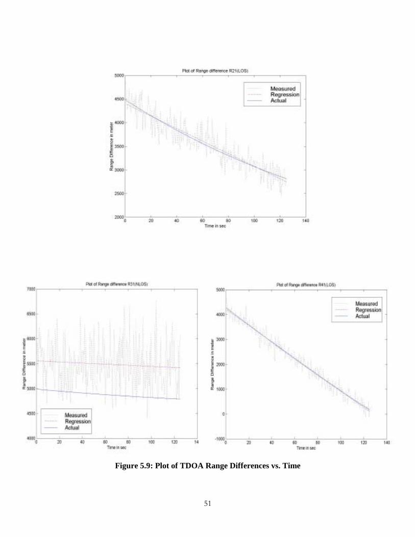
51

Figure 5.9: Plot of TDOA Range Differences vs. Time

52

5.3.2 Evaluation of the Estimator�s Performance for Position Estimation In the previous section we have demonstrated that the TDOA simulator is functioning properly.

Most of the position identification applications such as to inform about a road accident or a fire

incidence, require only the position estimates. Therefore the velocity of the mobile unit in the

simulator will be set to zero and the simulator�s output will be recorded at different mobile locations.

The estimator directly outputs the x �coordinate and the y-coordinate of the mobile. These values of

the estimates will be used to calculate the mean and variance of the estimates. Table 5.7 shows the

mean of the estimated positions as well as the range bias and the range standard deviation. CRLB is

also included to compare the standard deviation to the lower limit. The biased results are presented

on the assumption that BS#3 and BS#4 have NLOS with the MS.

Table 5.7: TDOA Estimator Performance at Different Mobile Location

MS Location MS Location (MS Far From

All BS)

MS Location (MS at the edge of

the cell) Real Position

( )00 , yx 600, 900 2000, 2000 600, 2500

Unbiased 599, 904 1999, 2008 599, 2523 Estimator

Mean( )yx ˆ,ˆ Biased 671, 594 1986, 1620 776, 2267

Unbiased 120.3, 102 162.5, 113.3 204.6, 108.5 Estimator Standard

Deviation( )yx σσ , Biased 130.4, 219 184.4, 284.8 222.6, 240.7

Unbiased 5 8 23 Range Bias, R

Biased 314 380 292

Unbiased 157.7 198 231.6 Range Standard

Deviation, σr Biased 254.9 339.3 327.8

Unbiased 158.8 197.2 202.6 CRLB Biased 268.8 345.7 319.8

53

The TDOA estimator performs well when the MS is considerably away from the controlling base

station. We mentioned before that, TDOA estimates suffer from high GDOP when the MS is close

to the controlling base station. The degradation of the TDOA estimates, when the MS is in close

proximity of the BS, is due to numerical instability of the equations that actually model the TDOA

triangulation. Table 5.8 shows the TDOA estimator�s performance at some locations when mobile is

very close to its controlling base station.

Table 5.8: TDOA Estimator�s Performance When MS is Very Close to the Controlling BS

MS

Location MS

Location

MS Location

MS Location

MS Location

Real Position

( )00 , yx 25, 25 50, 50 150, 150 200, 200 300, 300

Estimator Mean

( )yx ˆ,ˆ

44, 39 48, 59 148, 141 192, 188 291, 308

Estimator Standard Deviation

( )yx σσ ,

102, 98 97, 97 129, 108 124, 105 118, 112

Range Bias, R 23 10 9 14 12

Range Standard

Deviation, σr

141.7 137.4 167.7 162.4 162.7

CRLB 158.8 155 171.8 162.2 162.5

54

5.4 Implementation of Data Fusion Model in Position Location We have already discussed in Chapter 3 the data fusion model applicable to the PL problem. In this

section we will briefly discuss how the model has been simulated using MATLAB codes. The TOA

measurements have been simulated by first determining the true distances between the MS and the

base stations. Then the TOA range measurement model present in the Section 2.1.1 is used to

generate a complete TOA data. The TDOA measurements are generated from the TOA data and

hence in contrast to the real life situation, the TDOA data cannot be assumed to be independent of

the TOA data. Once again we should mention that the TOA estimator takes the smoothed TOA

measurements as its input, where as the TDOA estimator takes raw measurements as its input. The

raw TOA measurements of the TOA module are used to form additional TDOA data. In the first

level data fusion module, these converted TDOA data are combined with the original TDOA

measurements. The combined TDOA data is used as the input to the Taylor-Series Least Square

estimator, similar to the one implemented in the TDOA module. The means of both the TOA

estimates and the TDOA estimates are combined in the second level data fusion stage. In this stage,

the TOA estimate is granted as the original estimate and is updated with the additional TDOA

estimate. The level-four process chooses the best estimate among all the four estimates. In this

simulation, the final decision about the optimum estimate is made on the basis of estimators�

variances. The output of the estimator with lowest variance will be chosen as the best estimate in the

level-four process.

Tables 5.9, 5.10 and 5.11 show the different estimators� output at different MS locations. The tables

also indicate the decisions made at the level-four process of the data fusion architecture about the

best position estimates. Tables 5.12 and 5.13 represent estimators� output when the MS is close to its

controlling base station, BS#1. The results in the Tables 5.12 and 5.13 show that, although the first

level estimator range biases are minimum, the estimates are not chosen as the best estimates. This

reveals that, the present method of deciding best estimate, based on range standard deviation, needs

to be modified.

55

Table 5.9: Estimators� Output in Data Fusion Architecture at MS (600, 900)

TOA Estimator

TDOA Estimator

TOA/TDOA 1st level fusion

TOA/TDOA 2nd level fusion

Actual Position (x0, y0)

(600, 900) (600, 900) (600, 900) (600, 900)

Unbiased (708, 977) (613, 902) (621, 920) (706, 977) Estimator mean

( )yx ˆ,ˆ Biased - (1010,1113) (855, 1047) (710, 977)

Unbiased 17, 9 113, 105 97, 83 16.8, 9.1 Standard Deviation

( )yx σσ , Biased - 223, 144 161, 101 15.7, 22.3

Unbiased 132 14 29 131 Range bias R Biased - 462 294 134

Unbiased 19.3 154.7 128 19 Range Standard Deviation

σr Biased - 265.8 189 19

Unbiased • Choice

Biased •

56

Table 5.10: Estimators� Output in Data Fusion Architecture at MS (2000, 2000) TOA

Estimator TDOA

Estimator TOA/TDOA 1st level fusion


Actual Position (x0, y0) (2000,2000) (2000,2000) (2000,2000) (2000,2000)

Unbiased (2173,2104) (1988,2003) (2030,2021) (2167,2104) Estimator mean

( )yx ˆ,ˆ Biased - 2588, 2371 2385, 2240 2176, 2105


( )yx σσ , Biased - 344, 233 228, 153 19.4, 7.9


Unbiased 29 202 173 29 Range Standard Deviation

σr Biased - 416 274 29

Unbiased • Choice

Biased •

57

Table 5.11: Estimators� Output in Data Fusion Architecture at MS (600, 2500) TOA

Estimator TDOA




(600, 2500) (600,2500) (600,2500) (600,2500)

Unbiased (857, 2630) (612, 2585) (642, 2581) (854, 2628) Estimator mean

( )yx ˆ,ˆ Biased - 1109, 2778 957, 2682 857, 2634


( )yx σσ , Biased - 297, 172 202, 107 18.3, 32.1


Unbiased 32 185 143 31 Range Standard Deviation

σr Biased - 344 228 32

Unbiased • Choice

Biased •

58

Table 5.12: Estimators� Output with Unbiased Input at MS (25, 25)

TOA

Estimator TDOA



Actual

Position

(x0, y0) (25, 25) (25, 25) (25, 25) (25, 25)

Estimator mean

( )yx ˆ,ˆ (36, 18) (32, 17) (29, 22) (36, 18)

Standard Deviation

( )yx σσ , 7, 9 95, 100 70, 73 11, 8

Range bias R

13 11 5 13

Range Standard

Deviation σr 11 138 101 14

Choice •

59

Table 5.13: Estimators� Output with Unbiased Input at MS (150, 150)

TOA

Estimator TDOA

Estimator


TOA/TDOA2nd level fusion

Actual Position

(x0, y0) (150, 150) (150, 150) (150, 150) (150, 150)

Estimator mean

( )yx ˆ,ˆ (157, 133) (158, 156) (153, 146) (157, 133)

Standard Deviation

( )yx σσ , 7, 6 107, 105 84, 75 4, 8

Range bias R

19 10 5 19

Range Standard Deviation

σr

10 150 112 9

Choice •

5.5 Chapter Summary In this chapter, we have presented preliminary results showing the performance of TOA and TDOA

position determination for a typical cellular environment. Throughout these simulations, the TOA

measurements were normalized for NLOS propagation using the Wylie-Holtzman correction

method. In the next chapter, we show how this method may be extended to correct TDOA

measurements.

60

Chapter 6

TDOA Data Model and Extension of Wylie-Holtzman Algorithm to TDOA Ranges

In this chapter we will propose a data model that can be used to synthesize the TDOA range

measurements. We will also show that, the Wylie-Holtzman algorithm to the TOA range

measurements cannot be applied directly to the TDOA range measurements. We would also

propose and validate a proposed correction method by presenting some simulation results. At the

end of the chapter, the performance of the data fusion simulator with the corrected TOA and

TDOA measurements will be discussed.

6.1 Data Model for TDOA Range Measurements Initially we will assume that the controlling base station has a complete LOS with the MS. The range

difference between base stations with respect to the controlling base station is given by the equation

2.2. The range measurements Ri can be modeled according to equation 2.1. For our convenience we

will rewrite equation 2.1 below.

),()()( pipipii tNLOStntLR ++= (6.1)

where,

sight.-of-line-Non todueError error,t measuremen Standard

, BS and MSbetween distance True, ttimedifferent at tsmeasuremen of Sets

),1.....(2,1,0index timeSampleM,....2,1index BS

p

===

=−==

==

i

i

i

NLOSnLK

Kpi

Since we are assuming that the controlling base station has a complete LOS with the MS, therefore

the general form of range difference with respect to BS#1 is given by the equation 6.2.

)()()()()( 111 pippippii tNLOStntntLtLR +−+−= (6.2)

61

The standard noise has a zero mean Gaussian distribution. Therefore the expectation of

)()( 1 ppi tntn − is

[ ] [ ] [ ] 0 11 =−=− nEnEnnE ii .

The variance is given by

Therefore, when the controlling base station has LOS, the TDOA range differences can be modeled

as follows

)( )( )( 111 ppipii tNLOStntLR ++= , (6.3)

where,

( )sight.-of-line-Non todueError

,212.13 0,Nerrort measuremen Standard difference Range True

, ttimedifferent at tsmeasuremen of Sets),1.....(2,1,0index timeSample

M,....2,1index BS

1

1

p

=≈=

=

=−==

==

i

i

i

NLOSnLK

Kpi

The standard measurement noise has a zero mean Gaussian distribution with the standard deviation

of 212 meter. In a Line-of-Sight environment, the base station measures range differences in the

presence of the standard system measurement noise. There will be no Non-Line-of-Sight error

under that condition and NLOS (tp) in equation 6.3 can be set to zero. The mean and standard

deviation of NLOS noise will remain on the order of 513 meter and 436 meter, respectively. Even

when the controlling base station would have the NLOS, the TDOA range model would remain

same, except that an additional NLOS would appear in the equation 6.3. The distribution of the

NLOS error would then change and would have a different mean and standard deviation.

( )[ ] [ ][ ] [ ] [ ]

. 2

2

2

2

221

21

21

21

221

σσσ

=+=

++=

++=−

nnEnEnEnnnnEnnE

ii

iii

62

6.2 Simulation Model The simulation model, used to present results in the subsequent sections, would be almost same as

the one mentioned in section 5.1. The L parameter of the TDOA ranges would be measured using

the Euclidian distance approach. BS#1 is the controlling base station and is located at the center of

the coordinate system. The other three participating base stations are uniformly spaced around a

circle. The base stations configuration is same as the one depicted by the Figure 5.1.

6.3 Correction of TDOA Range Measurements Biased by NLOS Error In the previous section we mentioned that, when there is a complete LOS between the base stations

and the MS, the measured range differences would include the standard system measurement noise.

Under such condition the range differences would not be biased by the NLOS noise. However,

when there is an LOS of the MS with the controlling base station, but has NLOS between the MS

and the participating base stations, the measured range differences would definitely contain NLOS

error bias. The NLOS problem tends to be the key source of error in the range measurements [2].

First we would like to determine whether the range difference measurements contain the NLOS

error bias, and then would try to reduce the amount of bias as much as possible. This would enable

to determine the mobile coordinates more accurately by TDOA PL estimator even in the presence

of NLOS environment.

6.3.1 Identification of NLOS Bias in TDOA Range Measurements The NLOS bias in the TDOA range measurements can be identified if we have the a priori

knowledge of the standard deviation of the standard measurement error. At the controlling base

station, the range difference measurements are smoothed by polynomial regression. By comparing

the standard deviation of a sample statistic to the known standard deviation of that statistic under

the null hypothesis, we can determine the existence of an NLOS error bias in the measurements [2].

When there is a complete LOS between the MS and the base stations, the range measurements are

affected by the standard measurement error in a very predictable manner. In such circumstance, the

measured range difference would deviate from the true range difference by the standard deviation of

the standard measurement error )(1 pi tn . If we perform an Nth order polynomial fit to the measured

range differences, we can expect that,

63

where,

1iσ = Standard Deviation of the standard measurement error.

In the presence of the NLOS error, the measured range differences would deviate from the

smoothed curves, so that 11ˆ ii σσ >> . The large standard deviation will be used to differentiate

between the LOS case and the NLOS case.

6.3.2 Extension of the Wylie-Holtzman Algorithm to the TDOA Range Measurements In the presence of an NLOS environment, the measured range differences are corrupted by both the

standard measurement error and the NLOS error. We have modeled the TDOA ranges in the

section 6.1, and in equation 6.3 we have shown that, the standard measurement error and the NLOS

error can be modeled as a random variable. Equation 6.4 shows the range of the random variable.

iippii tNLOStn βαα +<+<− 2)()(2 1 (6.4)

Once we have the raw TDOA data, we can smooth the data by using an Nth order polynomial fit. It

is worth mentioning that the effect of the NLOS error is only to bias the data [2]. If we extend the

Wylie-Holtzman algorithm to the TDOA range measurements, then from the equation 6.4 we can

deduce that, the maximum deviation of the measured range difference below the smoothed curve

would be approximately i1 2- )( αpi tL . Therefore, by vertically displacing the smooth curve down

by ))()((max 11 pipi tRtS − and moving the curve up by 2αi would reduce the bias in the range

measurements introduced by the NLOS error. Now we will derive the expression for the TDOA

range correction from the Wylie-Holtzman algorithm given for TOA range correction.

According to equation 2.1

).()()()( pipipipi tNLOStntLtR ++= (6.4)

As we are assuming that BS#1 has LOS and ith BS has an NLOS, therefore range equation for BS#1

becomes

.)()()( 111 ppp tntLtR += (6.5)

If Sm(tp) is the smoothed version of Rm(tp), then according to Wylie-Holtzman algorithm, the

corrected ranges of equation 6.4 becomes

( ) ,)()(1ˆ 10

2111 i

K

ppipii tRtS

Kσσ ≅−= ∑

=

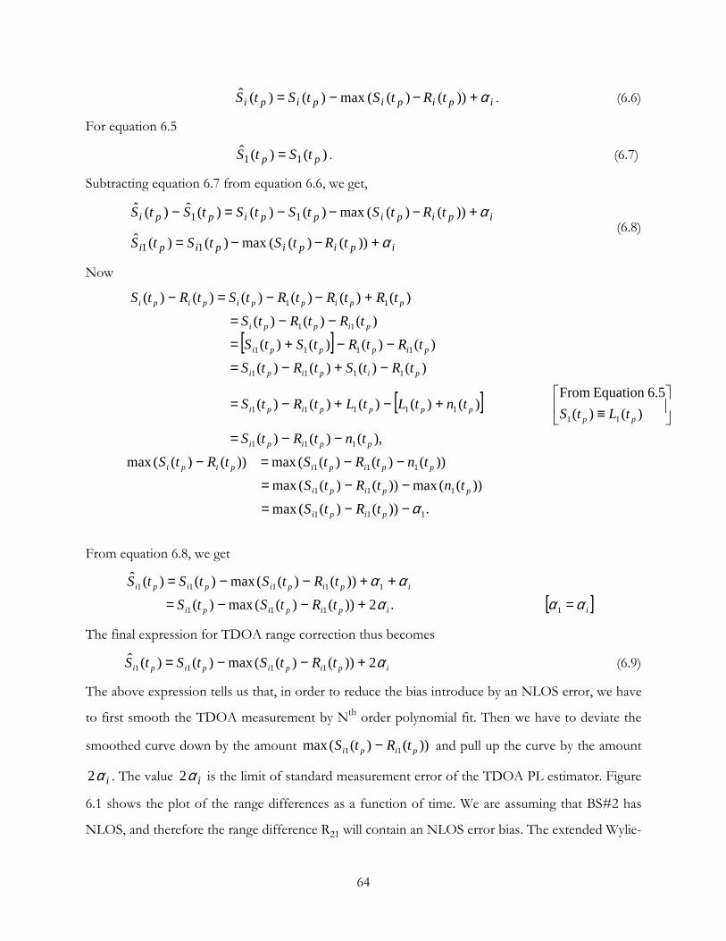
64

ipipipipi tRtStStS α+−−= ))()((max)()(ˆ . (6.6)

For equation 6.5

)()(ˆ11 pp tStS = . (6.7)

Subtracting equation 6.7 from equation 6.6, we get,

ipipipipi

ipipippippi

tRtStStS

tRtStStStStS

α

α

+−−=

+−−−=−

))()((max)()(ˆ

))()((max)()()(ˆ)(ˆ

11

11 (6.8)

Now

[ ]

[ ]

.))()((max

))((max))()((max ))()()((max ))()((max

),()()(

)()(6.5Equation From

)()()()()(

)()()()( )()()()(

)()()(

)()()()()()(

111

111

111

111

1111111

1111

1111

11

11

α−−=

−−=

−−=−

−−=

≡

+−+−=

−+−=

−−+=

−−=

+−−=−

pipi

ppipi

ppipipipi

ppipi

ppppppipi

pipipi

pipppi

pippi

ppippipipi

tRtStntRtS

tntRtStRtStntRtS

tLtStntLtLtRtS

tRtStRtStRtRtStS

tRtRtStRtRtRtStRtS

From equation 6.8, we get

[ ]iipipipi

ipipipipi

tRtStStRtStStS

ααααα

=+−−=

++−−=

1111

11111

.2))()((max)( ))()((max)()(ˆ

The final expression for TDOA range correction thus becomes

ipipipipi tRtStStS α2))()((max)()(ˆ1111 +−−= (6.9)

The above expression tells us that, in order to reduce the bias introduce by an NLOS error, we have

to first smooth the TDOA measurement by Nth order polynomial fit. Then we have to deviate the

smoothed curve down by the amount ))()((max 11 pipi tRtS − and pull up the curve by the amount

iα2 . The value iα2 is the limit of standard measurement error of the TDOA PL estimator. Figure

6.1 shows the plot of the range differences as a function of time. We are assuming that BS#2 has

NLOS, and therefore the range difference R21 will contain an NLOS error bias. The extended Wylie-

65

Holtzman algorithm is applied to the range difference. We have also plotted the corrected smoothed

curve of the range measurements so that the curve can be compared to the plot of true range

differences.

Figure 6.1: Plot of Range Differences vs. time (With Extended W-H Algorithm)

66

From the plot it is evident that the Wylie-Holtzman algorithm, applicable to the TOA

measurements, is not directly applicable to the TDOA measurements. Therefore, in order to reduce

the effect of NLOS noise in the TDOA measurements, we have to adopt a different kind of

correction method. In the following section we are proposing a new correction method, which

would provide better improvement compared to that obtained by the extended Wylie-Holtzman

algorithm.

6.3.3 Proposed Correction Method We are still assuming that the standard measurement noise has zero mean Gaussian distribution with

standard deviation of 212.13 meters. Once again we should remind that we are still assuming that

the controlling base station BS#1 has a complete LOS with the MS. Therefore if the MS has an

NLOS with the Ith base station, the corresponding range differences will contain a single NLOS

error. The NLOS error will have a single sided Gaussian distribution with mean of 513 meter and

standard deviation of 409 meter. In the previous section, we have mentioned that the effect of an

NLOS error is only to bias the measured range differences. Since the NLOS error has only positive

support ranges, therefore the data will contain a positive bias. On the average, the measurement will

have a positive bias almost equal to the mean of the NLOS error. Therefore we propose that,

instead of using equation 6.9 for reducing the NLOS error bias in the TDOA ranges, we will shift

the raw measurements downwards by the value equal to the mean of the error. Figure 6.2 shows the

improvement of the range differences obtained by applying the proposed algorithm. As only the

BS#2 has an NLOS with the MS, the range difference R21 contains the error bias, and therefore

correction method is applied only to these measurements. From the figure it is also evident that, the

averages of the measurements R31 and R41 lie close to the true values. We can also conclude from

the figure that, the proposed algorithm can offer significant improvement in eliminating the bias in

the TDOA data.

6.4 Validation of Correction Method Applied to TDOA Measurements Figure 6.2 shows plot of estimated range of the MS from the BS#1 as a function of signal-to-noise

ratio. From the figure we find that, for high SNR higher than 22 dB the estimates obtained from the

GCC method is close to the estimates where TDOA range measurements are synthesized by the

proposed model. For computational simplicity, we will use the model where the TDOA range

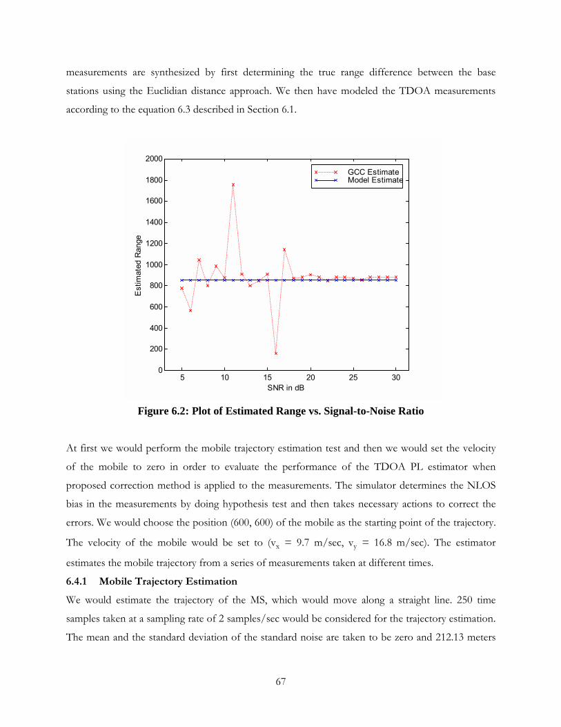
67

measurements are synthesized by first determining the true range difference between the base

stations using the Euclidian distance approach. We then have modeled the TDOA measurements

according to the equation 6.3 described in Section 6.1.

5 10 15 20 25 300

200

400

600

800

1000

1200

1400

1600

1800

2000

SNR in dB

Est

imat

ed R

ange

GCC Estimate Model Estimate

Figure 6.2: Plot of Estimated Range vs. Signal-to-Noise Ratio

At first we would perform the mobile trajectory estimation test and then we would set the velocity

of the mobile to zero in order to evaluate the performance of the TDOA PL estimator when

proposed correction method is applied to the measurements. The simulator determines the NLOS

bias in the measurements by doing hypothesis test and then takes necessary actions to correct the

errors. We would choose the position (600, 600) of the mobile as the starting point of the trajectory.

The velocity of the mobile would be set to (vx = 9.7 m/sec, vy = 16.8 m/sec). The estimator

estimates the mobile trajectory from a series of measurements taken at different times.

6.4.1 Mobile Trajectory Estimation We would estimate the trajectory of the MS, which would move along a straight line. 250 time

samples taken at a sampling rate of 2 samples/sec would be considered for the trajectory estimation.

The mean and the standard deviation of the standard noise are taken to be zero and 212.13 meters

68

respectively. The values used for an NLOS error are the ones mentioned in the section 6.3.2. Since

BS#1 is the controlling base station, all the range differences are calculated with respect to the range

of the mobile from the BS#1. In this simulation we have assumed that the BS#1 has a full LOS

whereas the BS#2 has an NLOS. Therefore the range difference R21 would contain the NLOS error

bias and the proposed correction method would be applied to the R21 measurements to reduce the

bias introduced by the error. Due to the NLOS error, the standard deviation of the R21

measurements would be much higher than the standard deviation of the R31 and R41 measurements.

The table 6.1 shows the standard deviation of the range measurements with the above mentioned

base station configuration. These standard deviations of the range differences are used for

hypothesis testing in determining the presence of an NLOS error in the measured TDOA ranges.

The threshold value for hypothesis testing is taken to be 350 meter. From the table, it is evident that

the TDOA simulator is able to detect the presence of the NLOS bias in the range measurements R21

and would therefore take necessary steps to reduce the effect of the bias in the measurements. The

figure 6.3 shows the output of the TDOA PL estimator with different kind of inputs. The dashed

line indicates the real mobile trajectory; the dotted line shows the estimated mobile trajectory when

the biased raw TDOA data is fed as the input to the estimator. The solid line represents the

estimated trajectory with proposed correction method applied to the TDOA measurements. The

dotted line represents this trajectory. From the figure we can conclude that our proposed correction

method indeed provides significant improvement in determining the MS position location in the

Non-Line-Of-Sight environment.

6.4.2 TDOA PL Estimator�s Performance with Corrected TDOA Measurements We will assume that the mobile is stationary in order to evaluate the estimator�s performance with

corrected TDOA ranges. Therefore, for the simulation results of this section, we will set the velocity

of the mobile to zero. Table 6.2 shows the simulator�s performance at different MS location. The

estimator estimates the x-coordinate and the y-coordinate of the mobile with 250 samples at each

location. The 250 estimates are used to determine the mean and variance of the estimator output.

The CRLB is included in the table to compare the range standard deviation to the theoretical limit.

The uncorrected results are presented, assuming that the BS#2 has NLOS with the MS. The range

bias in the table indicates the remarkable improvement obtained by the proposed correction

method. We will now see the application of the simulator to the data fusion architecture.

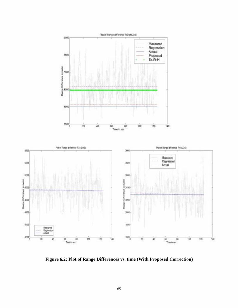
69

Figure 6.2: Plot of Range Differences vs. time (With Proposed Correction)

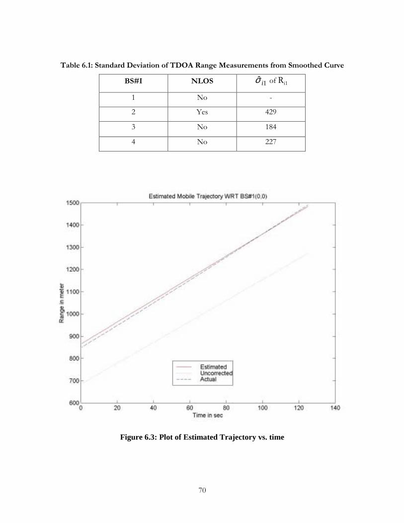
70


BS#I NLOS 1ˆ iσ of Ri1

1 No -

2 Yes 429

3 No 184

4 No 227

Figure 6.3: Plot of Estimated Trajectory vs. time

71

Table 6.2: TDOA Estimator Performance at Different Mobile Location

MS Location MS Location (MS Far From

All BS)

MS Location (MS at the edge of

the cell) Real Position

( )00 , yx 600, 900 2000, 2000 600, 2500

Corrected 569, 896 1951, 2015 571, 2533 Estimator

Mean( )yx ˆ,ˆ Uncorrected 299, 937 1548, 2045 318, 2524

Corrected 276, 133 344, 138 313, 142 Estimator Standard

Deviation( )yx σσ , Uncorrected 228, 116 327, 128 267, 146

Corrected 31 52 43 Range Bias, R

Uncorrected 303 454 283

Corrected 306 371 344 Range Standard

Deviation, σr Uncorrected 256 351 304

Corrected 333 367 348 CRLB Uncorrected 328 361 348

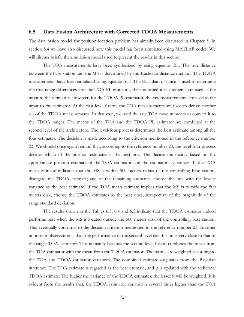
72

6.5 Data Fusion Architecture with Corrected TDOA Measurements The data fusion model for position location problem has already been discussed in Chapter 3. In

section 5.4 we have also discussed how this model has been simulated using MATLAB codes. We

will discuss briefly the simulation model used to present the results in this section.

The TOA measurements have been synthesized by using equation 2.1. The true distance

between the base station and the MS is determined by the Euclidian distance method. The TDOA

measurements have been simulated using equation 6.3. The Euclidian distance is used to determine

the true range differences. For the TOA PL estimator, the smoothed measurements are used as the

input to the estimator. However, for the TDOA PL estimator, the raw measurements are used as the

input to the estimator. At the first level fusion, the TOA measurements are used to derive another

set of the TDOA measurements. In that case, we used the raw TOA measurements to convert it to

the TDOA ranges. The means of the TOA and the TDOA PL estimator are combined at the

second level of the architecture. The level-four process determines the best estimate among all the

four estimates. The decision is made according to the criterion mentioned in the reference number

23. We should once again remind that, according to the reference number 23, the level-four process

decides which of the position estimates is the best one. The decision is mainly based on the

approximate position estimate of the TOA estimator and the estimators� variances. If the TOA

mean estimate indicates that the MS is within 500 meters radius of the controlling base station,

disregard the TDOA estimate; and of the remaining estimates, choose the one with the lowest

variance as the best estimate. If the TOA mean estimate implies that the MS is outside the 500

meters disk, choose the TDOA estimates as the best ones, irrespective of the magnitude of the

range standard deviation.

The results shown in the Tables 6.3, 6.4 and 6.5 indicate that the TDOA estimator indeed

performs best when the MS is located outside the 500 meters disk of the controlling base station.

This eventually conforms to the decision criterion mentioned in the reference number 23. Another

important observation is that, the performance of the second level data fusion is very close to that of

the single TOA estimator. This is mainly because the second level fusion combines the mean from

the TOA estimator with the mean from the TDOA estimator. The means are weighted according to

the TOA and TDOA estimator variances. The combined estimate originates from the Bayesian

inference. The TOA estimate is regarded as the best estimate, and it is updated with the additional

TDOA estimate. The higher the variance of the TDOA estimates, the lesser it will be weighted. It is

evident from the results that, the TDOA estimator variance is several times higher than the TOA

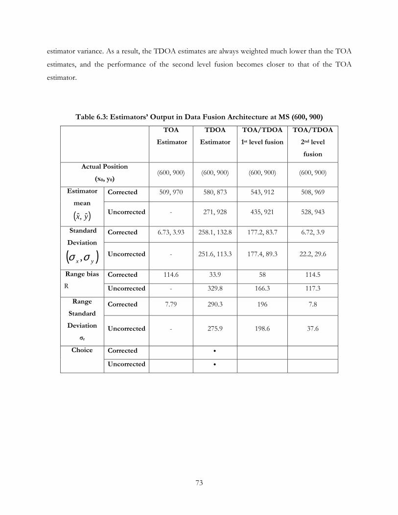
73

estimator variance. As a result, the TDOA estimates are always weighted much lower than the TOA

estimates, and the performance of the second level fusion becomes closer to that of the TOA

estimator.


TOA Estimator

TDOA Estimator




(600, 900) (600, 900) (600, 900) (600, 900)

Corrected 509, 970 580, 873 543, 912 508, 969 Estimator mean

( )yx ˆ,ˆ Uncorrected - 271, 928 435, 921 528, 943

Corrected 6.73, 3.93 258.1, 132.8 177.2, 83.7 6.72, 3.9 Standard Deviation

( )yx σσ , Uncorrected - 251.6, 113.3 177.4, 89.3 22.2, 29.6

Corrected 114.6 33.9 58 114.5 Range bias R Uncorrected - 329.8 166.3 117.3

Corrected 7.79 290.3 196 7.8 Range Standard Deviation

σr Uncorrected - 275.9 198.6 37.6

Corrected • Choice

Uncorrected •

74


TOA Estimator

TDOA Estimator




(2000, 2000) (2000, 2000) (2000, 2000) (2000, 2000)



Corrected 9.5, 12.1 345.3, 136.9 237.2, 94.2 9.51, 12 Standard Deviation

( )yx σσ , Uncorrected - 321.4, 124 230, 85.6 10.3, 7

Corrected 101.6 31.6 100.4 101.1 Range bias R Uncorrected - 457.3 316.5 108.1

Corrected 15.39 371.4 255.2 15.38 Range Standard Deviation

σr Uncorrected - 344.5 245.4 12.5


Uncorrected •

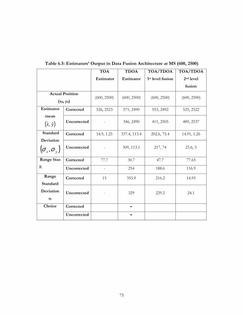
75


TOA Estimator

TDOA Estimator




(600, 2500) (600, 2500) (600, 2500) (600, 2500)




( )yx σσ , Uncorrected - 309, 113.1 217, 74 23.6, 5

Corrected 77.7 30.7 47.7 77.65 Range bias R Uncorrected - 254 188.6 116.9

Corrected 15 355.9 216.2 14.95 Range Standard Deviation

σr Uncorrected - 329 229.2 24.1


Uncorrected •

76


TOA

Estimator TDOA




(50, 50) (50, 50) (50, 50) (50, 50)

Estimator mean

( )yx ˆ,ˆ 8, 78 466, 532 46, 53 46, 79

Standard Deviation

( )yx σσ , 6, 1 21, 20 62, 93 6, 1

Range bias R

51 637 5 29

Range Standard Deviation σr 7 29 112 6

Choice •

77


TOA

Estimator TDOA




(150, 150) (150, 150) (150, 150) (150, 150)

Estimator mean

( )yx ˆ,ˆ 52, 246 29, 363 105, 175 51, 287

Standard Deviation

( )yx σσ , 1, 7 32, 10 52, 122 1, 6

Range bias R

138 245 51 169

Range Standard Deviation σr 8 34 133 7

Choice •

78

The results in the Tables 6.3 to 6.7 are based on the assumption that only the BS#2 has an NLOS,

and all other base stations have complete LOS with the MS. Now we will present the data fusion

estimator output with the base station configuration that all the participating BS�s have NLOS with

the MS. The results will represent the estimators� performance under an extreme harsh

environmental condition.

Table 6.8: Data Fusion Architecture Performance at MS (600, 900) with all BS having NLOS

TOA Estimator

TDOA Estimator




(600, 900) (600, 900) (600, 900) (600, 900)



Corrected 9.4, 15.2 310.5, 245.6 219.5, 168 9.36, 15.18 Standard Deviation


Corrected 66.5 82.3 113.5 66.4 Range bias R Uncorrected - 246 151.4 105.6

Corrected 17.86 395.9 276.4 17.8 Range Standard Deviation

σr Uncorrected - 289 211.8 26.7

Corrected ● Choice

Uncorrected ●

79

Table 6.9: Data Fusion Architecture Performance at MS (2000,2000) with all BS having NLOS

TOA Estimator

TDOA Estimator




(2000,2000) (2000,2000) (2000,2000) (2000,2000)



Corrected 30.9, 12.94 377, 280.7 248.8, 192 30.8, 12.93 Standard Deviation


Corrected 136.7 78.7 128.8 135.5 Range bias R Uncorrected - 569.3 343.8 159.1

Corrected 33.52 470 314.3 33.44 Range Standard Deviation

σr Uncorrected - 399.8 307.12 16.9


Uncorrected ●

80

Table 6.10: Data Fusion Architecture Performance at MS (600,2500) with all BS having NLOS

TOA Estimator

TDOA Estimator




(600,2500) (600,2500) (600,2500) (600,2500)





Corrected 97 54.4 138.2 96.8 Range bias R Uncorrected - 378.7 256.8 116.3

Corrected 21.9 467 332.6 21.8 Range Standard Deviation

σr Uncorrected - 368.2 289.3 23.7


Uncorrected ●

The results once again indicate the amount of improvement obtained by the proposed correction

method even under a harsh environmental condition. Although in most cases when the MS is

located outside the 500 meters disk of the controlling base station, the TDOA estimator performs

best, there are some cases when we found that first level data fusion performs best. One of such

cases is shown in the table 6.8. We find that although the range bias of the second level data fusion

is minimum, yet the output of the TDOA estimator is selected to be best estimator since the MS is

located outside the 500 meters disk of the controlling base station. This once again indicates that

attention must be given to decide optimum estimate in the data fusion architecture. In this research

81

work we did not focus on finding an optimum estimate in the data fusion architecture. Further

research should be carried along this avenue.

Tables 6.11 to 6.13 represents data fusion architecture performance where the TDOA data are

generated using the GCC method. The channel models described in sections 4.2 and 4.3 are used in

these simulation results. In CDMA system, automatic power control is used. The automatic power

control causes the MS transmitter to transmit at the higher power when the MS is far from the

controlling base station. As a result, the received signal power is stronger at the base stations far

away from the MS. This is one of the reasons why TDOA estimator performance improves in the

CDMA networks as the MS moves away from the controlling base station. The results indicate to

another fact, that the data fusion architecture for PL promises to show better performance in the

CDMA system.

Table 6.11: Data Fusion Architecture Performance at MS (600,2500) in GCC with 25 dB SNR

TOA

Estimator

TDOA

Estimator

TOA/TDOA

1st level fusion

TOA/TDOA

2nd level fusion

Actual

Position

(x0, y0)

(600, 900) (600, 900) (600, 900) (600, 900)

Estimator

mean

( )yx ˆ,ˆ

641, 833 588, 843 602, 838 641, 833

Standard

Deviation

( )yx σσ , 14, 19.3 160, 244 94, 173 14, 19.27

Range bias

R 78 58 61 78

Range

Standard

Deviation σr

23.9 292.4 197.1 23.8

Choice ●

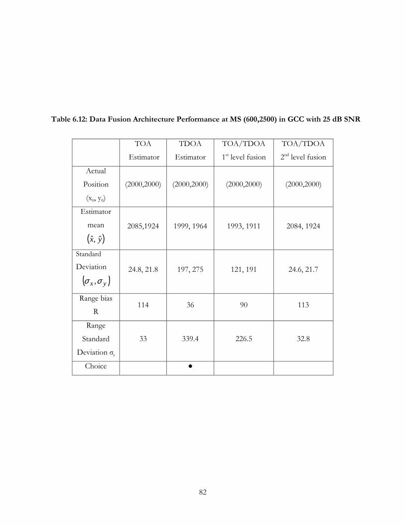
82


TOA

Estimator

TDOA

Estimator

TOA/TDOA

1st level fusion

TOA/TDOA

2nd level fusion

Actual

Position

(x0, y0)

(2000,2000) (2000,2000) (2000,2000) (2000,2000)

Estimator

mean

( )yx ˆ,ˆ

2085,1924 1999, 1964 1993, 1911 2084, 1924

Standard

Deviation

( )yx σσ , 24.8, 21.8 197, 275 121, 191 24.6, 21.7

Range bias

R 114 36 90 113

Range

Standard

Deviation σr

33 339.4 226.5 32.8

Choice ●

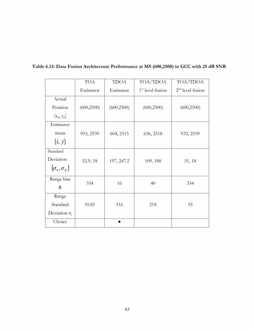
83


TOA

Estimator

TDOA

Estimator

TOA/TDOA

1st level fusion

TOA/TDOA

2nd level fusion

Actual

Position

(x0, y0)

(600,2500) (600,2500) (600,2500) (600,2500)

Estimator

mean

( )yx ˆ,ˆ

953, 2539 604, 2515 636, 2518 932, 2539

Standard

Deviation

( )yx σσ , 52.9, 18 197, 247.2 109, 188 51, 18

Range bias

R 354 16 40 334

Range

Standard

Deviation σr

55.85 316 218 55

Choice ●

84

Chapter 7

Conclusions Position estimation of the mobile users in the cellular phone networks is becoming an important

issue as the deadline for meeting the FCC requirements approaches. A precise position estimation

capability will allow the service providers not only to satisfy the FCC requirements but also to offer

new services to stay competitive. The RF based techniques are found to be practically viable for the

cellular system. This research work provides an overview of different RF based position location

techniques, Data Fusion for PL and evaluates the suitability of these structures for E-911 service. In

the revised standards for the Phase-II location accuracy and reliability, the FCC regulates that for

network-based solutions, all the carriers must be able to locate a mobile with an accuracy of 100

meters in 67 percent of all the calls and 300 meters for 95 percent of all the calls. The main objective

of this research is to develop enhanced techniques for reaching these goals.

7.1 Summary of Results In Chapter 1, we briefly discussed the background of the E-911 service, presenting an overview of

modified handset techniques and unmodified handset techniques. Unmodified handset based TOA

and TDOA techniques are found to be the most attractive solutions, since these methods can be

implemented with minimal changes in the network hardware and software.

Chapter 2 discussed the system independent algorithms of TOA and TDOA based PL

techniques. The core part of this research work is based on the results of the examinations

conducted by Silventoinen and Rantalainen [4]. According to the work of [4], the Non-Line-Of-

Sight propagation is the prime source of error for the TOA measurements. The NLOS error adds a

positive bias to the measurements and needs to be removed in order to get an acceptable PL

accuracy. The Wylie-Holtzman algorithm suggests a method to eliminate the NLOS bias from the

measurements. The chapter includes a discussion on the basic principle of the Wylie-Holtzman

algorithm as well. Once the presence of the NLOS bias in the TOA measurements is determined,

the Wylie-Holtzman algorithm is applied to eliminate the bias, and then the corrected measurements

are used as the input to the TOA estimator. The Taylor-Series Least Square method is used for both

the TOA and the TDOA estimator to estimate the position location of the mobile. The Taylor-

85

Series is used to linearize the non-linear range equations results from the GCC range measurement.

The least square error method is used to solve the resulting set of linear equations locally, and

therefore the composite method is called the Taylor Series Least Square method. In practice, the

TDOA range measurements are calculated using the GCC method. Two base stations receive signals

from the MS and the received signals are correlated to determine the TDOA of the signal relative to

one base station. The location of the first peak at the correlator output gives an approximate TDOA

of the signal. The Circular Error Probability describes the figure of merit of the position estimate.

The estimator�s performance largely depends on the geometrical configuration of the base station

and the mobile unit. The TDOA estimator suffers from a large GDOP when the MS is located close

to the BS. In order to measure the accuracy of the position estimator, the RMS position error of the

estimator is compared to the CRLB, which is the theoretical limit for the unbiased estimator. The

CRLB actually indicates how optimally the estimation process is working.

In Chapter 3, we discussed about the general JDL data fusion architecture and its application

to the PL solution. The JDL data fusion architecture is a conceptual model that identifies and

categorizes the process, functions, and techniques applicable to data fusion. When same source data

is gathered by using multiple independent sensors, the data would have statistical gain over single

source data. The main feature of the data fusion architecture is that, decisions are made at different

hierarchical levels. One thing should be clearly understood that, the levels are classified according to

the type of data used as the input to the decision processor; a higher numbered level does not

indicate better decision stage. In general, the source-of-information, human-computer interaction,

source processing, level-1 processing, level-2 processing, level-3 processing, and level-4 processing

conceptualize the JDL model. Information may be a sensor data or a priori information from the

database. The data fusion process must work with the data that is most pertinent to the existing

condition and at the same time deduce the processing load. Level-1 operates on the raw data and

performs multiple functions. We briefly discussed the hybrid model proposed by Hall [14] that

combines level one and level two fusion based on the JDL model. The chapter also discussed the

data fusion model for position location estimation proposed by Kleine-Ostmann and Bell [23]. The

model combines the raw TOA and TDOA data at the first level data fusion. Since only the similar

kind of data can be fused, the TOA data are converted to the corresponding TDOA data before

fusing at the first level. The control process, which is the second level fusion, makes the final choice

about the best estimate. The second level data fusion utilizes the Bayesian Inferences to improve an

estimate with known statistics once new data is available. The probability distribution of the old

86

estimate is updated depending on the probability distribution of the new data and the amount of

data available.

Chapter 4 included a discussion on the received signal models, path loss models and the

additive white Gaussian noise channel. The range measurements between the base station and the

mobile unit are linearly proportional to the TOA measurements. When there is a complete LOS

between the BS and the MS, only the standard measurement noise affects the true range

measurements. Otherwise, the NLOS error has the predominant effect on the range measurements.

The path loss model used indicates the average received signal power that decreases logarithmically

with the distance. The near-field effects otherwise may alter the reference path loss.

Chapter-5 presents the results for the TOA estimator, the TDOA estimator and the data

fusion approach. The TOA data was modeled according to the measurement statistics presented in

the reference number [4]. Basically, the chapter presents simulation results that validate the

performance of the TOA and the TDOA estimator. The chapter also includes the results to indicate

the performance of the data fusion simulator with corrected TOA and uncorrected TDOA

measurements. The results are useful to compare the improvement obtained by the proposed

TDOA correction method presented in Chapter 6.

Finally, Chapter 6 presents the results of the basic contribution of this research work. In this chapter

we have shown how a data model for the TDOA range measurements can be derived from the

TOA range models presented in the reference number [4]. The chapter includes a discussion on how

the NLOS error bias incorporated in the TDOA range measurements can be reduced to get

acceptable location identification accuracy under the non-line-of-sight environmental condition.

7.2 Contributions of this Research Work The basic contributions of this research work are as follows:

• The new data model for the TDOA range measurements

• Development of the algorithm to reduce the NLOS error bias in the TDOA range

measurements

• Evaluation of the Data Fusion Architecture of PL proposed in the reference number [23]

The data model presented in this research is derived from the knowledge of the measurements

obtained by Silventoinen and Rantalainen [4]. The model can be used to synthesize the TDOA range

measurements, even under non-line-of-sight conditions. The range difference between base stations

87

with respect to the controlling base station is given by the equation 2.2. The standard measurement

noise has a zero mean Gaussian distribution with standard deviation of 212 meter. In an LOS

environment, the base station measures range difference in the presence of the standard system

measurement noise. Depending on the base stations configuration, the mean and standard deviation

of the NLOS error will vary. We have derived the equations under the assumption that the

controlling base station has a complete LOS with the MS all the time. Under such conditions, the

mean and variance of the NLOS error is found to be 513 meter and 436 meter respectively. The

NLOS error tends to be the key source of error in the measurements, and therefore needs to be

eliminated in order to get acceptable accuracy from the TDOA measurements.

The proposed correction method requires that, at first the NLOS error bias have to be

detected in the TDOA data. The bias in the measurements can be identified if we have the a priori

knowledge of the standard deviation of the standard measurement noise. In the presence of the

NLOS error, the measured range differences would deviate from the smoothed curves so that the

standard deviation is much greater than the standard deviation of the standard measurement noise.

The proposed correction method is based on the fact that the effect of NLOS error is to

positively bias the measured range differences. Since the standard measurement noise has zero mean

Gaussian distribution, hence on the average the measurements will have a positive bias equal to the

mean of the NLOS error. So to reduce the effect of the bias, the raw measurements need to be

shifted downward by the value equal to the mean of the NLOS error. The results shown the Table

6.2 indicates significant improvement obtained by the new correction method applied to the TDOA

data in the NLOS environment. We have also applied the proposed data model and the correction

method to the data fusion architecture for PL proposed by Kleine-Ostmann and Bell [23]. The

performance of the architecture indicates that the model is potential to meet the FCC requirements

with improved accuracy. The simulation results show that, the TDOA estimate is usually better than

the TOA estimate, but deteriorates faster under an unfavorable geometric configuration of the base

stations and the MS. The data fusion architecture for PL is capable of coping with the geometric

dilution of precision. The unique property of the model is that, it evaluates two types of input data

and tries to achieve better estimate than a single estimate. The best choice of the estimates is made

at the level four of the architecture. According to Kleine-Ostmann and Bell [23], the decision is

based on the approximate position estimate of the TOA method and the estimator variance. The

estimate that is regarded to be the best is the final data fusion process output. If the TOA mean

estimate indicates that the MS is in a radius of 500 meter around the controlling base station, the

88

TDOA estimate is discarded. Under such circumstances, the one with the lowest variance is taken as

the final estimate. If the TOA estimate indicates that the MS is located outside the 500 meters radius

circle around the controlling base station, then the TDOA estimate is considered to be the best

solution. Although most of the simulation results of DF architecture in this research conform to this

decision criterion, results of some instances contradict the criterion. For example, in Table 6.6, we

find that, although the range bias of the first level fusion is minimum among all the range biases, the

second level output is still chosen as the best estimate. Therefore we conclude that the data fusion

architecture for PL is indeed suitable for providing solution to the E-911 PL problem with improved

accuracy, but the decision criterion is not optimum, and thus requires some modifications.

7.3 Directions for Future Research The simulation results have shown that both the TOA and the TDOA techniques are eligible for the

E-911 PL solution. However, the algorithms have to be tested under real world conditions. The

TOA and TDOA data need to be recorded in different terrains so that the statistics can be evaluated

properly. The correction algorithms largely depend on the statistical parameters, configured at

different environmental conditions.

The work done in this research can be extended in different ways. We have derived the

TDOA data model assuming that the controlling base has a complete line-of-sight with the MS. The

model needs to be tuned when the controlling base station and the participating base stations have

an NLOS with the MS. Analysis should be carried out to find the mean and variance of the NLOS

error under such circumstance. Testing is required to verify the proposed correction method with

the real TDOA measurements obtained from the GCC method. We have simulated the data fusion

model with an ideal base station configuration, and with a simple channel model. It will be

interesting to see how the proposed DF model performs with a non-ideal base station arrangement,

since cellular layout in the real situations seldom follow the ideal hexagonal layout. In all the

simulations we have assumed that the mobile is stationary at a particular location. Investigation can

be pursued to see the estimators� perform in the fading channel.

Another avenue of progress would be to delve into the decision criterion used in the control process

of the data fusion architecture. Finding an optimum decision criterion in the DF architecture would

be a research topic alone.

One of the interesting observations made in this research was the divergence problem of the TDOA

estimator. Although it is more of a mathematical problem rather than an engineering problem, yet it

89

will be interesting to find out at what condition the Taylor Series Least Square estimator suffers

from the convergence problem.

The position location algorithms require participation of at least three base stations in the process.

The requirements of the network for position determination exceed the requirements for

communications. The practical cells are laid in a fashion such that it is unfavorable for the position

determination algorithm. However, according to Silventoinen and Rantalainen, the accessibility is

only a problem in the rural environment. If the decision is made to implement the TOA and the

TDOA solutions, the requirements for location estimation must be taken into account in the

network planning. Once the hardware of the base stations is modified to implement the position

estimation, then from an application standpoint, it is important to know exactly at which layer of the

processing stack this process is executed, and how much additional processing load would it require

for the switching.

90

Bibliography

[1] T. S. Rappaport, J. H. Reed, B. D. Woerner, �Position Location Using Wireless

Communications on Highways of the Future�, IEEE Communications Magazine,

vol. 34, no. 10, pp. 33-41, October 1996.

[2] M. P. Wylie, J. Holtzman, �The Non-line of Sight Problem in Mobile Location

Estimation�, International Conf. On Universal Personal Communications, pp. 827-831, 1996.

[3] D. J. Torrieri, �Statistical Theory of Passive Location System �, IEEE Transaction on

Aerospace and Electronic Systems, AES vol. 20, no. 2, pp.183-198, March 1984.

[4] M. I. Silventoinen, T. Rantalainen, �Mobile Station Emergency Location in GSM�, IEEE

International Conf. On Personal Wireless Communications, pp. 232-238, February 1996.

[5] T. K. Ostmann, �Position Estimation in Cellular CDMA Phone Networks�, An Independent

Study report submitted at Virginia Polytechnic Institute and State University, August 1999.

[6] M. Aatique, �Evaluation of TDOA Technique for Position Location in CDMA System�,

Master’s Thesis at Virginia Polytechnic Institute and State University, September 1997.

[7] W. H. Foy, �Position Location Solutions by Taylor-Series Estimation�, IEEE

Transactions on Aerospace and Electronic Systems, vol. 12, no. 2, pp. 187-194. March 1976.

[8] Y. T. Chan, K. C. Ho, �A Simple and Efficient Estimator For Hyperbolic Location�,

IEEE Transactions on Signal Processing, vol. 42, no. 8, pp 1905-1915, August 1994.

[9] �FCC Report and Order and Further Notice of Proposed Rule Making�, FCC Docket 96-

264, June 1996.

[10] E. Hepsaydir, W. Yates, �Performance Analysis of Positioning Using Existing CDMA

91

System�, IEEE Position Location and Navigation Systems, pp. 190-192, 1994.

[11] M.Aatique, G.A. Mizusawa, B.D. Woerner, �Performance of Hyperbolic Position

Location Techniques in Code Division Multiple Access�. Proc. 9th Annual Conf. On Wireless

Comm. T.R Labs and IEEE Canada, July 9-11, 1997.

[12] C.H. Knapp, G.C. Carter, �The Generalized Correlation Method for Estimation of Time

Delay�, IEEE Transaction on Acoustics, Speech and Signal Processing, vol. ASSP-24, no. 4, pp. 320-

327, August 1976.

[13] S. Bancroft, �An Algebraic Solution of the GPS Equations�, IEEE Transaction on Aerospace

and Electronic Systems, vol. AES-21, pp. 56-59, January 1985.

[14] D.L. Hall, J. Llinas, �An Introduction to Multisensor Data Fusion�, Proceedings of IEEE,

85(1): pp. 6 � 23, January 1997.

[15] H.W. Sorenson, �Least-Square Estimation: From Gauss to Kalman�, IEEE Spectrum, pp. 63-

68, July 1970.

[16] C.T. Zahn, �Graph-theoretical Methods for Detecting and Describing Gestalt Cluster�,

IEEE Trans. Computers, vol. C-20, January 1971.

[17] Y. Bar-Shalom, E. Tse, �Tracking in a Cluttered Environment with Probabilistic Data

Association�, Automatica, vol. 2, pp. 451- 460, September 1975.

[18] C. Bowman, private communication to D.L. Hall, October 1995.

[19] Leon W. Couch, �Digital and Analog Communication Systems�, Prentice Hall, Upper

Saddle River, NJ, 1997.

[20] T. S. Rappaport, �Wireless Communications Principles and Practice�, Prentice Hall PTR,

Upper Saddle River, NJ 07458.

92

[21] G. A. Mizusawa, �Performance of Hyperbolic Position Location Techniques for Code

Division Multiple Access�, Master’s Thesis at Virginia Polytechnic Institute and State University,

August 16, 1996.

[22] W. H. Tranter, K. S. Shanmugan, K. L. Kosbar and T. S. Rappaport, �Computer-Aided Design

and Analysis of Communication Systems�, Prentice Hall, 2000.

[23] Kleine-Ostmann, T. and Bell, A., �A Data Fusion Architecture for Enhanced Position

Estimation in Wireless Networks,� submitted to GLOBECOM 2000.

[24] John S. Bay, Fundamentals of Linear State Space Systems, McGraw-Hill, 1998

[25] J. Kennedy et al., �Characterization of the Cellular Radio Environment �, Proc. 2nd Workshop

on Smart Antennas in Wireless Mobile Communication, Stanford University, July 20-21, 1995

[26] G. R. Iverson, Bayesian Statistical Inference, Sage, Beverly Hills, CA 1984

[27] H. C. Schau and A. Z. Robinson, �Passive Source Localization Employing Intersecting

Spherical Surfaces from Time-of-Arrival Differences�, IEEE Transactions on Acoustics, Speech,

and Signal Processing, vol. ASSP-35, no.8, pp. 1223-1225, August 1987

[28] H. B. Lee, �Accuracy Limitations of Hyperbolic Multilateration Systems�, IEEE Transaction

on Aerospace and Electronic Systems, vol. AES-114, no. 1, pp. 16-29, January 1975

[29] H. Stark and J. W. Woods, Probability, Random Processes, and Estimation Theory for Engineers,

Prentice-Hall Inc., 2nd edition, 1994

[30] Peter Clarke, �Cell Phone Positioned for New Services�, Electronic Engineering Times, vol. 30,

no. 25, pp. 6, January 20, 1997

[31] Radio Commissions Report, October 18, 1999.

93

Vita

Rahman I. Reza was born in Dhaka, Bangladesh, November 11, 1973. He received a Bachelor of

Engineering degree in Electrical Engineering from Bangladesh University of Engineering and

Technology (BUET), Dhaka, Bangladesh, 1997. He joined the graduate program at Virginia

Polytechnic Institute and State University in August 1998, and has been a member of the Mobile and

Portable Radio Research Group since January 1999. His research efforts in MPRG have focused on

position location techniques for CDMA systems.

data fusion for improved toa/tdoa position determination in

Documents