data intensive query processing for semantic …lkhan/papers/thesishussain.pdf · data intensive...
TRANSCRIPT

DATA INTENSIVE QUERY PROCESSING FOR SEMANTIC WEB DATA
USING HADOOP AND MAPREDUCE
by
Mohammad Farhan Husain
APPROVED BY SUPERVISORY COMMITTEE:
Dr. Bhavani Thuraisingham, Co-Chair
Dr. Latifur Khan, Co-Chair
Dr. Murat Kantarcioglu
Dr. Kevin Hamlen

Copyright c© 2011
Mohammad Farhan Husain
All Rights Reserved R©

To the Almighty
DATA INTENSIVE QUERY PROCESSING FOR SEMANTIC WEB DATA
USING HADOOP AND MAPREDUCE
by
MOHAMMAD FARHAN HUSAIN, B.S.
DISSERTATION
Presented to the Faculty of
The University of Texas at Dallas
in Partial Fulfillment
of the Requirements
for the Degree of
DOCTOR OF PHILOSOPHY IN COMPUTER SCIENCE
THE UNIVERSITY OF TEXAS AT DALLAS
May, 2011
PREFACE
This dissertation was produced in accordance with guidelines which permit the inclusion as
part of the dissertation the text of an original paper or papers submitted for publication.
The dissertation must still conform to all other requirements explained in the ”Guide for the
Preparation of Master’s Theses and Doctoral Dissertations at The University of Texas at
Dallas.” It must include a comprehensive abstract, a full introduction and literature review
and a final overall conclusion. Additional material (procedural and design data as well as
descriptions of equipment) must be provided in sufficient detail to allow a clear and precise
judgment to be made of the importance and originality of the research reported.
It is acceptable for this dissertation to include as chapters authentic copies of papers already
published, provided these meet type size, margin and legibility requirements. In such cases,
connecting texts which provide logical bridges between different manuscripts are mandatory.
Where the student is not the sole author of a manuscript, the student is required to make an
explicit statement in the introductory material to that manuscript describing the student’s
contribution to the work and acknowledging the contribution of the other author(s). The
signatures of the Supervising Committee which precede all other material in the dissertation
to the accuracy of this statement.
v

ACKNOWLEDGEMENTS
Firstly, I would like to dedicate my appreciation to my research advisors, Dr. Bhavani
Thuraisingham and Dr. Latifur Khan, for devoting their precious time and efforts to guide
and support me. Without their invaluable advice and patient assistance, it would not be
possible for me to pursue my Ph.D. degree and complete this dissertation.
I would like to than my committee members, Dr. Murat Kantarcioglu and Dr. Kevin
Hamlen, for the helpful suggestions and discussions, and contributing their time generously
in serving on my proposal and dissertation defense.
I would like to sincerely thank Pankil Doshi, James McGlothlin and Dr. Mohammad M.
Masud for working with me in solving problems and implementing and running experiments
during the course of my Ph.D. Their inspirations and encouragement kept me going during
my work for Ph.D.
I would like to thank my wife and my parents for their deepest love and unconditional
support over all these years. I would not have been where I am today without their love,
understanding and efforts to hold me up during my research. My wife, Marzia Murshed,
deserves special mention here as she was the one who most constantly was at my side,
providing the support, care and encouragement that I was in dire need of.
Finally, I thank the Almighty who gave me the knowledge, patience and perseverance that
allowed me to complete this doctoral degree. I would like to dedicate this work to Him.
April, 2011
vi
DATA INTENSIVE QUERY PROCESSING FOR SEMANTIC WEB DATA
USING HADOOP AND MAPREDUCE
Publication No.
Mohammad Farhan Husain, Ph.D.
The University of Texas at Dallas, 2011
Supervising Professors: Dr. Bhavani Thuraisingham, Co-ChairDr. Latifur Khan, Co-Chair
Semantic Web is an emerging area to augment human reasoning. Various technologies are
being developed in this arena which have been standardized by the World Wide Web Consor-
tium (W3C). One such standard is the Resource Description Framework (RDF). Semantic
Web technologies can be utilized to build efficient and scalable systems for Cloud Comput-
ing. With the explosion of semantic web technologies, large RDF graphs are common place.
This poses significant challenges for the storage and retrieval of RDF graphs. Current frame-
works do not scale for large RDF graphs and as a result do not address these challenges.
In this dissertation, we describe a framework that we built using Hadoop, an open source
distributed file system supporting MapReduce programming paradigm, to store and retrieve
large numbers of RDF triples by exploiting the cloud computing paradigm. We describe a
scheme to store RDF data in Hadoop Distributed File System. SPARQL (SPARQL Protocol
and RDF Query Language) is a language to query RDF data. We present an algorithm which
can rewrite some SPARQL queries to equivalent simpler ones leveraging the storage scheme.
More than one Hadoop job (the smallest unit of execution in Hadoop) may be needed to
vii

answer a query because a single triple pattern in a query cannot simultaneously take part in
more than one join in a single Hadoop job. To determine the jobs, we present multiple algo-
rithms, based on greedy and exhaustive search approach, to generate query plan to answer a
SPARQL query. We extend those algorithms to generate query plans for complex SPARQL
queries with OPTIONAL blocks. We use Hadoop’s MapReduce framework to answer the
queries. Our results show that we can store large RDF graphs in Hadoop clusters built with
cheap commodity class hardware. Furthermore, we show that our framework is scalable and
efficient and can handle large amounts of RDF data, unlike traditional approaches.
viii
TABLE OF CONTENTS
PREFACE . . . . . . . . . . . . . . . . . . . . . . . . . . . . . . . . . . . . . . . . . . . . . . . . . . . . . . . . . . . . . . . . . . . . . . . . . . . . v
ACKNOWLEDGEMENTS . . . . . . . . . . . . . . . . . . . . . . . . . . . . . . . . . . . . . . . . . . . . . . . . . . . . . . . . . . . . vi
ABSTRACT . . . . . . . . . . . . . . . . . . . . . . . . . . . . . . . . . . . . . . . . . . . . . . . . . . . . . . . . . . . . . . . . . . . . . . . . . . vii
LIST OF TABLES . . . . . . . . . . . . . . . . . . . . . . . . . . . . . . . . . . . . . . . . . . . . . . . . . . . . . . . . . . . . . . . . . . . . xiii
LIST OF FIGURES. . . . . . . . . . . . . . . . . . . . . . . . . . . . . . . . . . . . . . . . . . . . . . . . . . . . . . . . . . . . . . . . . . . xiv
CHAPTER 1. INTRODUCTION . . . . . . . . . . . . . . . . . . . . . . . . . . . . . . . . . . . . . . . . . . . . . . . . . . . . 1
CHAPTER 2. RESEARCH BACKGROUND . . . . . . . . . . . . . . . . . . . . . . . . . . . . . . . . . . . . . . . . 7
2.1 MapReduce Programming Paradigm . . . . . . . . . . . . . . . . . . . . . . . . . . . . . . . . . . . . . . . . 7
2.1.1 MapReduce in Data Mining . . . . . . . . . . . . . . . . . . . . . . . . . . . . . . . . . . . . . . . . . 8
2.1.2 MapReduce in Semantic Web . . . . . . . . . . . . . . . . . . . . . . . . . . . . . . . . . . . . . . . . 9
2.2 Semantic Web Frameworks . . . . . . . . . . . . . . . . . . . . . . . . . . . . . . . . . . . . . . . . . . . . . . . . 9
CHAPTER 3. SYSTEM ARCHITECTURE . . . . . . . . . . . . . . . . . . . . . . . . . . . . . . . . . . . . . . . . . 13
3.0.1 Data Generation and Storage . . . . . . . . . . . . . . . . . . . . . . . . . . . . . . . . . . . . . . . . 13
3.0.2 File Organization . . . . . . . . . . . . . . . . . . . . . . . . . . . . . . . . . . . . . . . . . . . . . . . . . . 14
3.0.3 Predicate Split (PS) . . . . . . . . . . . . . . . . . . . . . . . . . . . . . . . . . . . . . . . . . . . . . . . . 15
3.0.4 Predicate Object Split (POS) . . . . . . . . . . . . . . . . . . . . . . . . . . . . . . . . . . . . . . . . 15
3.0.5 Example Data . . . . . . . . . . . . . . . . . . . . . . . . . . . . . . . . . . . . . . . . . . . . . . . . . . . . . 17
3.0.6 Binary Format . . . . . . . . . . . . . . . . . . . . . . . . . . . . . . . . . . . . . . . . . . . . . . . . . . . . . 18
ix
CHAPTER 4. MAP-REDUCE FRAMEWORK . . . . . . . . . . . . . . . . . . . . . . . . . . . . . . . . . . . . . . 19
4.1 Query Rewriting . . . . . . . . . . . . . . . . . . . . . . . . . . . . . . . . . . . . . . . . . . . . . . . . . . . . . . . . . 20
4.2 Input Files Selection . . . . . . . . . . . . . . . . . . . . . . . . . . . . . . . . . . . . . . . . . . . . . . . . . . . . . 23
4.3 Cost Estimation and Plan Generation for Query Processing . . . . . . . . . . . . . . . . . . . . 25
4.3.1 Ideal Model . . . . . . . . . . . . . . . . . . . . . . . . . . . . . . . . . . . . . . . . . . . . . . . . . . . . . . . 27
4.3.2 The GenerateBestPlan Algorithm . . . . . . . . . . . . . . . . . . . . . . . . . . . . . . . . . . . . 29
4.3.3 Heuristic Model . . . . . . . . . . . . . . . . . . . . . . . . . . . . . . . . . . . . . . . . . . . . . . . . . . . . 38
4.3.4 The DetermineJobs Algorithm . . . . . . . . . . . . . . . . . . . . . . . . . . . . . . . . . . . . . . . 43
4.3.5 The Relaxed-Bestplan Algorithm . . . . . . . . . . . . . . . . . . . . . . . . . . . . . . . . . . . . . 47
4.3.6 Breaking Ties by Summary Statistics . . . . . . . . . . . . . . . . . . . . . . . . . . . . . . . . . 57
4.4 Queries with Optional Blocks . . . . . . . . . . . . . . . . . . . . . . . . . . . . . . . . . . . . . . . . . . . . . . 58
4.5 MapReduce Join Execution . . . . . . . . . . . . . . . . . . . . . . . . . . . . . . . . . . . . . . . . . . . . . . . 64
CHAPTER 5. SUMMARY STATISTICS . . . . . . . . . . . . . . . . . . . . . . . . . . . . . . . . . . . . . . . . . . . . 67
5.1 Selectivity of Individual Triple Patterns . . . . . . . . . . . . . . . . . . . . . . . . . . . . . . . . . . . . . 67
5.1.1 Selectivity of Individual Triple Patterns with Bound Components . . . . . . . . . 67
5.1.2 Selectivity of Individual Triple Patterns with Unbound Components . . . . . . 68
5.2 Selectivity of Joined Triple Patterns . . . . . . . . . . . . . . . . . . . . . . . . . . . . . . . . . . . . . . . . 69
5.2.1 Selectivity of Joined Triple Patterns with Bound/Unbound Predicate . . . . . . 69
CHAPTER 6. RESULTS . . . . . . . . . . . . . . . . . . . . . . . . . . . . . . . . . . . . . . . . . . . . . . . . . . . . . . . . . . . . 75
6.1 Data Sets . . . . . . . . . . . . . . . . . . . . . . . . . . . . . . . . . . . . . . . . . . . . . . . . . . . . . . . . . . . . . . . 75
6.2 Baseline Frameworks . . . . . . . . . . . . . . . . . . . . . . . . . . . . . . . . . . . . . . . . . . . . . . . . . . . . . 75
6.3 Experimental Setup . . . . . . . . . . . . . . . . . . . . . . . . . . . . . . . . . . . . . . . . . . . . . . . . . . . . . . 76
6.3.1 Hardware . . . . . . . . . . . . . . . . . . . . . . . . . . . . . . . . . . . . . . . . . . . . . . . . . . . . . . . . . 76
6.3.2 Software . . . . . . . . . . . . . . . . . . . . . . . . . . . . . . . . . . . . . . . . . . . . . . . . . . . . . . . . . . 76
6.4 Evaluation . . . . . . . . . . . . . . . . . . . . . . . . . . . . . . . . . . . . . . . . . . . . . . . . . . . . . . . . . . . . . . 76
6.4.1 Comparison with Baseline Frameworks . . . . . . . . . . . . . . . . . . . . . . . . . . . . . . . . 78
x
6.4.2 Experiment with Number of Reducers . . . . . . . . . . . . . . . . . . . . . . . . . . . . . . . . . 82
6.4.3 Experiment with PigLatin . . . . . . . . . . . . . . . . . . . . . . . . . . . . . . . . . . . . . . . . . . . 83
6.5 Validation . . . . . . . . . . . . . . . . . . . . . . . . . . . . . . . . . . . . . . . . . . . . . . . . . . . . . . . . . . . . . . 86
CHAPTER 7. ACCESS CONTROL . . . . . . . . . . . . . . . . . . . . . . . . . . . . . . . . . . . . . . . . . . . . . . . . . 87
7.1 Access Control Level Descriptions . . . . . . . . . . . . . . . . . . . . . . . . . . . . . . . . . . . . . . . . . . 88
7.1.1 Access Token Assignment . . . . . . . . . . . . . . . . . . . . . . . . . . . . . . . . . . . . . . . . . . . 91
7.1.2 Final output of an Agent’s ATs . . . . . . . . . . . . . . . . . . . . . . . . . . . . . . . . . . . . . . 93
7.1.3 Assumptions . . . . . . . . . . . . . . . . . . . . . . . . . . . . . . . . . . . . . . . . . . . . . . . . . . . . . . 93
7.1.4 Conflicts . . . . . . . . . . . . . . . . . . . . . . . . . . . . . . . . . . . . . . . . . . . . . . . . . . . . . . . . . . 94
7.2 Proposed Architecture with Access Control . . . . . . . . . . . . . . . . . . . . . . . . . . . . . . . . . . 95
7.3 Policy Enforcement . . . . . . . . . . . . . . . . . . . . . . . . . . . . . . . . . . . . . . . . . . . . . . . . . . . . . . 98
7.3.1 Query Rewriting . . . . . . . . . . . . . . . . . . . . . . . . . . . . . . . . . . . . . . . . . . . . . . . . . . . 98
7.3.2 Embedded Enforcement . . . . . . . . . . . . . . . . . . . . . . . . . . . . . . . . . . . . . . . . . . . . . 99
7.3.3 Post-processing Enforcement . . . . . . . . . . . . . . . . . . . . . . . . . . . . . . . . . . . . . . . . . 100
7.4 Experimental Setup and Results . . . . . . . . . . . . . . . . . . . . . . . . . . . . . . . . . . . . . . . . . . . 101
7.4.1 Validation . . . . . . . . . . . . . . . . . . . . . . . . . . . . . . . . . . . . . . . . . . . . . . . . . . . . . . . . . 102
CHAPTER 8. CONCLUSION AND FUTURE WORK. . . . . . . . . . . . . . . . . . . . . . . . . . . . . . . 104
8.1 Conclusion . . . . . . . . . . . . . . . . . . . . . . . . . . . . . . . . . . . . . . . . . . . . . . . . . . . . . . . . . . . . . . 104
8.2 Limitations . . . . . . . . . . . . . . . . . . . . . . . . . . . . . . . . . . . . . . . . . . . . . . . . . . . . . . . . . . . . . 105
8.3 Future Work . . . . . . . . . . . . . . . . . . . . . . . . . . . . . . . . . . . . . . . . . . . . . . . . . . . . . . . . . . . . 106
8.3.1 Sophisticated Query Model . . . . . . . . . . . . . . . . . . . . . . . . . . . . . . . . . . . . . . . . . . 106
8.3.2 Experiment with Number of Reducers . . . . . . . . . . . . . . . . . . . . . . . . . . . . . . . . . 106
8.3.3 Indexing . . . . . . . . . . . . . . . . . . . . . . . . . . . . . . . . . . . . . . . . . . . . . . . . . . . . . . . . . . 107
8.3.4 Different Types of SPARQL Queries . . . . . . . . . . . . . . . . . . . . . . . . . . . . . . . . . . 107
8.3.5 Using Hive and HBase . . . . . . . . . . . . . . . . . . . . . . . . . . . . . . . . . . . . . . . . . . . . . . 109
8.3.6 Inferencing . . . . . . . . . . . . . . . . . . . . . . . . . . . . . . . . . . . . . . . . . . . . . . . . . . . . . . . . 110
xi

REFERENCES . . . . . . . . . . . . . . . . . . . . . . . . . . . . . . . . . . . . . . . . . . . . . . . . . . . . . . . . . . . . . . . . . . . . . . . 110
VITA
xii
LIST OF TABLES
3.1 Data size at various steps for 1000 universities . . . . . . . . . . . . . . . . . . . . . . . . . . . . 16
3.2 Sample data for LUBM Query 9 . . . . . . . . . . . . . . . . . . . . . . . . . . . . . . . . . . . . . . . . 17
4.1 Plans for SP 2Bench Query 5(b) . . . . . . . . . . . . . . . . . . . . . . . . . . . . . . . . . . . . . . . . 39
4.2 2 Job Plan vs. 3 Job plan . . . . . . . . . . . . . . . . . . . . . . . . . . . . . . . . . . . . . . . . . . . . . 42
4.3 Iteration 1 Calculations . . . . . . . . . . . . . . . . . . . . . . . . . . . . . . . . . . . . . . . . . . . . . . . 46
4.4 Iteration 1 - After choosing X . . . . . . . . . . . . . . . . . . . . . . . . . . . . . . . . . . . . . . . . . . 46
4.5 Iteration 2 Calculations . . . . . . . . . . . . . . . . . . . . . . . . . . . . . . . . . . . . . . . . . . . . . . . 46
4.6 Example Data . . . . . . . . . . . . . . . . . . . . . . . . . . . . . . . . . . . . . . . . . . . . . . . . . . . . . . . 58
4.7 Example Query Result . . . . . . . . . . . . . . . . . . . . . . . . . . . . . . . . . . . . . . . . . . . . . . . . 58
5.1 Example Data . . . . . . . . . . . . . . . . . . . . . . . . . . . . . . . . . . . . . . . . . . . . . . . . . . . . . . . 73
5.2 Summary Statistics Creation Example . . . . . . . . . . . . . . . . . . . . . . . . . . . . . . . . . . . 73
6.1 Comparison with RDF-3X . . . . . . . . . . . . . . . . . . . . . . . . . . . . . . . . . . . . . . . . . . . . . 77
6.2 Query Runtimes for LUBM and SP2B Dataset . . . . . . . . . . . . . . . . . . . . . . . . . . . . 77
6.3 Query Runtimes Comparison . . . . . . . . . . . . . . . . . . . . . . . . . . . . . . . . . . . . . . . . . . . 85
7.1 EEMap Output and EEReduce Input . . . . . . . . . . . . . . . . . . . . . . . . . . . . . . . . . . . 100
xiii
LIST OF FIGURES
3.1 The System Architecture . . . . . . . . . . . . . . . . . . . . . . . . . . . . . . . . . . . . . . . . . . . . . . 14
3.2 Partial LUBM Ontology (are denotes subClassOf relationship) . . . . . . . . . . . . . 17
4.1 NCMRJ and CMRJ Example . . . . . . . . . . . . . . . . . . . . . . . . . . . . . . . . . . . . . . . . . . 26
4.2 Join and Inverted Graph for Query 12 . . . . . . . . . . . . . . . . . . . . . . . . . . . . . . . . . . . 31
4.3 Graph Coloring for Query 12 . . . . . . . . . . . . . . . . . . . . . . . . . . . . . . . . . . . . . . . . . . . 36
4.4 Join and Inverted Graph for SP 2Bench Query 5(b) . . . . . . . . . . . . . . . . . . . . . . . 39
4.5 Graph for Query 12 in Iteration 1 . . . . . . . . . . . . . . . . . . . . . . . . . . . . . . . . . . . . . . . 45
4.6 Graph for Query 12 in Iteration 2 . . . . . . . . . . . . . . . . . . . . . . . . . . . . . . . . . . . . . . . 45
4.7 The (partial) graph for the running example query with the initial state and
all states adjacent to it. . . . . . . . . . . . . . . . . . . . . . . . . . . . . . . . . . . . . . . . . . . . . . . . 51
4.8 Operator Graph for (a) Example Query, (b) Modified Example Query . . . . . . . 59
4.9 Operator Graph for (a) SP2B Query 6, (b) SP2B Query 7 . . . . . . . . . . . . . . . . . . 62
6.1 Response time of LUBM Query 2 . . . . . . . . . . . . . . . . . . . . . . . . . . . . . . . . . . . . . . . 81
6.2 Response time of LUBM Query 9 . . . . . . . . . . . . . . . . . . . . . . . . . . . . . . . . . . . . . . . 82
6.3 Response time of LUBM Query 12 . . . . . . . . . . . . . . . . . . . . . . . . . . . . . . . . . . . . . . 83
6.4 Query Runtimes for SP2B Queries . . . . . . . . . . . . . . . . . . . . . . . . . . . . . . . . . . . . . . 84
6.5 Query Time vs. Number of Reducers . . . . . . . . . . . . . . . . . . . . . . . . . . . . . . . . . . . . 84
6.6 Query Runtimes . . . . . . . . . . . . . . . . . . . . . . . . . . . . . . . . . . . . . . . . . . . . . . . . . . . . . . 85
7.1 The shaded gray area can be viewed by an agent having 1 access level. . . . . . . 90
7.2 A sample RDF ontology and ontology instance. . . . . . . . . . . . . . . . . . . . . . . . . . . . 92
7.3 The System Architecture . . . . . . . . . . . . . . . . . . . . . . . . . . . . . . . . . . . . . . . . . . . . . . 97
xiv

7.4 Performance measurement of takesCourse scenario. The Y-axis represents
runtimes in milliseconds and X-axis shows set of data-set size. . . . . . . . . . . . . . . 101
7.5 Performance measurement of displayTeachers scenario. The Y-axis repre-
sents runtimes in milliseconds and X-axis shows set of data-set size. . . . . . . . . . 103
xv
CHAPTER 1
INTRODUCTION
Cloud computing is an emerging paradigm in the IT and data processing commu-
nities. Enterprizes utilize cloud computing service to outsource data maintenance, which
can result in significant financial benefits. Businesses store and access data at remote lo-
cations in the ”cloud”. As the popularity of cloud computing grows, the service providers
face ever increasing challenges. They have to maintain huge quantities of heterogenous data
while providing efficient information retrieval. Thus the key emphasis for cloud computing
solutions is scalability and query efficiency.
Semantic Web technologies are being developed to present data in standardized way
such that such data can be retrieved and understood by both human and machine. His-
torically, web pages are published in plain html files which are not suitable for reasoning.
Instead, the machine treats these html files as a bag of keywords. Researchers are develop-
ing Semantic Web technologies that have been standardized to address such inadequacies.
The most prominent standards are Resource Description Framework† (RDF) and SPARQL
Protocol and RDF Query Language† (SPARQL). RDF is the standard for storing and rep-
resenting data and SPARQL is a query language to retrieve data from an RDF store. Cloud
Computing systems can utilize the power of these Semantic Web technologies to provide the
user with capability to efficiently store and retrieve data for data intensive applications.
†http://www.w3.org/TR/rdf-primer†http://www.w3.org/TR/rdf-sparql-query
1
2
Semantic web technologies could be especially useful for maintaining data in the
cloud. Semantic web technologies provide the ability to specify and query heterogenous data
in a standardized manner. Moreover, via OWL (Web Ontology Language) ontologies, dif-
ferent schemas, classes, data types and relationships can be specified without sacrificing the
standard RDF/SPARQL interface. Conversely, cloud computing solutions could be of great
benefit to the semantic web community. Semantic web datasets are growing exponentially.
More than any other arena, in the web domain, scalability is paramount. Yet, high speed
response time is also vital in the web community. We believe that the cloud computing
paradigm offers a solution that can achieve both of these goals.
Existing commercial tools and technologies do not scale well in Cloud Computing
settings. Researchers have started to focus on these problems recently. They are proposing
systems built from the scratch. In (Wang, Wu, Gao, Li, and Ooi 2010), researchers propose
an indexing scheme for a new distributed database† which can be used as a Cloud system.
When it comes to semantic web data such as RDF, we are faced with similar challenges.
With storage becoming cheaper and the need to store and retrieve large amounts of data,
developing systems to handle billions of RDF triples requiring tera bytes of disk space is no
longer a distant prospect. Researchers are already working on billions of triples (Rohloff,
Dean, Emmons, Ryder, and Sumner 2007; Newman, Hunter, Li, Bouton, and Davis 2008).
Competitions are being organized to encourage researchers to build efficient repositories†.
At present, there are just a few frameworks (e.g. RDF-3X (Neumann and Weikum 2008),
Jena (Carroll, Dickinson, Dollin, Reynolds, Seaborne, and Wilkinson 2004; McBride 2002),
Sesame† (Broekstra, Kampman, and van Harmelen 2002), BigOWLIM (Kiryakov, Ognyanov,
and Manov 2005)) for Semantic Web technologies, and these frameworks have limitations for
†http://www.comp.nus.edu.sg/~epic/†http://challenge.semanticweb.org†http://www.openrdf.org
3
large RDF graphs. Therefore, storing a large number of RDF triples and efficiently querying
them is a challenging and important problem.
A distributed system can be built to overcome the scalability and performance prob-
lems of current Semantic Web frameworks. Databases are being distributed in order to
provide such scalable solutions. However, to date, there is no distributed repository for stor-
ing and managing RDF data. Researchers have only recently begun to explore the problems
and technical solutions which must be addressed in order to build such a distributed sys-
tem. One promising line of investigation involves making use of readily available distributed
database systems or relational databases. Such database systems can use relational schema
for the storage of RDF data. SPARQL queries can be answered by converting them to SQL
first (Chebotko, Lu, and Fotouhi 2009; Chong, Das, Eadon, and Srinivasan 2005; Cyga-
niak 2005). Optimal relational schemas are being probed for this purpose (Abadi, Marcus,
Madden, and Hollenbach 2007). The main disadvantage with such systems is that they are
optimized for relational data. They may not perform well for RDF data, especially because
RDF data are sets of triples† (an ordered tuple of three components called subject, predicate
and object respectively) which form large directed graphs. In a SPARQL query, any number
of triple patterns† can join on a single variable† which makes a relational database query
plan complex. Performance and scalability will remain a challenging issue due to the fact
that these systems are optimized for relational data schemata and transactional database
usage.
Yet another approach is to build a distributed system for RDF from scratch. Here,
there will be an opportunity to design and optimize a system with specific application to
RDF data. In this approach, the researchers would be reinventing the wheel.
†http://www.w3.org/TR/rdf-concepts/#dfn-rdf-triple†http://www.w3.org/TR/rdf-sparql-query/#defn_TriplePattern†http://www.w3.org/TR/rdf-sparql-query/#defn_QueryVariable
4
Instead of starting with a blank slate, we propose to build a solution with a generic
distributed storage system which utilizes a Cloud Computing platform. We then propose to
tailor the system and schema specifically to meet the needs of semantic web data. Finally,
we propose to build a semantic web repository using such a storage facility.
Hadoop† is a distributed file system where files can be saved with replication. It is
an ideal candidate for building a storage system. Hadoop features high fault tolerance and
great reliability. In addition, it also contains an implementation of the MapReduce(Dean and
Ghemawat 2008) programming model, a functional programming model which is suitable for
the parallel processing of large amounts of data. Through partitioning data into a number of
independent chunks, MapReduce processes run against these chunks, making parallelization
simpler. Moreover, the MapReduce programming model facilitates and simplifies the task
of joining multiple triple patterns.
In this dissertation, we will describe a schema to store RDF data in Hadoop, and
we will detail a solution to process queries against this data. In the preprocessing stage, we
process RDF data and populate files in the distributed file system. This process includes
partitioning and organizing the data files and executing dictionary encoding. Our schema
facilitates rewriting some queries to their equivalent simpler. We will present an algorithm
for the rewriting.
We will then detail a query engine for information retrieval. We will specify exactly
how SPARQL queries will be satisfied using MapReduce programming. Specifically, we
must determine the Hadoop ”jobs” that will be executed to solve the query. We will present
three algorithms that produce a query plan for a SPARQL query. Two of them are greedy
algorithms and one is an exhaustive search algorithm. One of the greedy algorithms is an
approximation algorithm using heuristics, but the worst case has a reasonable upper bound.
†http://hadoop.apache.org

5
The exhaustive algorithm can use any cost model and choose the best plan for a query using
that cost model. with the minimal number of Hadoop jobs. We also have another algorithm
which can handle complex SPARQL queries with OPTIONAL blocks. In this algorithm, we
can use any of the three algorithms previously mentioned as a sub-routine.
Finally, we will utilize two standard benchmark datasets to run experiments. We will
present results for dataset ranging from 0.1 to over 6.6 billion triples. We will show that
our solution is exceptionally scalable. We will show that our solution outperforms leading
state-of-the-art semantic web repositories, using standard benchmark queries on very large
datasets.
Our contributions are as follows:
1. We design a storage scheme to store RDF data in Hadoop distributed file system
(HDFS†).
2. We propose an algorithm for query rewriting leveraging our schema.
3. We propose a greedy algorithm which generates query plans by choosing most number
of possible joins at each step.
4. We propose an exhaustive search algorithm based on a two coloring scheme. The
algorithm can use any cost function to choose the best plan.
5. We propose an algorithm that is guaranteed to provide a query plan whose cost is
bounded by the log of the total number of variables in the given SPARQL query. It
uses summary statistics for estimating join selectivity to break ties.
†http://hadoop.apache.org/core/docs/r0.18.3/hdfs_design.html

6
6. We propose an algorithm which can generate query plans for complex SPARQL queries
with OPTIONAL blocks by using any of the three previously mentioned algorithms as
a sub-routine.
7. We build a framework which is highly scalable and fault tolerant and supports data
intensive query processing.
8. We demonstrate that our approach performs better than state-of-the-art semantic web
repositories, using standard benchmark queries on very large datasets.
The remainder of this dissertation is organized as follows: in Chapter 2, we investigate
related work. In Chapter 3, we discuss our system architecture. In Chapter 4, we discuss how
we answer a SPARQL query. In Chapter 5, we present the summary statistics we gather
to break ties while generating a query plan. In Chapter 6, we present the results of our
experiments. Finally, in Chapter 8, we draw some conclusions and discuss areas we have
identified for improvement in the future.
CHAPTER 2
RESEARCH BACKGROUND
In this chapter, we will first investigate research related to MapReduce. Next, we will
discuss works related to the semantic web.
2.1 MapReduce Programming Paradigm
MapReduce, though a programming paradigm, is rapidly being adopted by researchers. This
technology is becoming increasingly popular in the community which handles large amounts
of data. It is the most promising technology to solve the performance issues researchers are
facing in Cloud Computing. In (Abadi 2009), Abadi discusses how MapReduce can satisfy
most of the requirements to build an ideal Cloud DBMS. Researchers and enterprizes are
using MapReduce technology for web indexing, searches and data mining.
Google uses MapReduce for web indexing, data storage and social networking (Chang,
Dean, Ghemawat, Hsieh, Wallach, Burrows, Chandra, Fikes, and Gruber 2006). Yahoo!
uses MapReduce extensively in their data analysis tasks (Olston, Reed, Srivastava, Kumar,
and Tomkins 2008). IBM has successfully experimented with a scale-up scale-out search
framework using MapReduce technology (Moreira, Michael, Da Silva, Shiloach, Dube, and
Zhang 2007). In a recent work (Das, Sismanis, Beyer, Gemulla, Haas, and McPherson 2010),
they have reported how they integrated Hadoop and System R. Teradata did a similar work
by integrating Hadoop with a parallel DBMS (Xu, Kostamaa, and Gao 2010). Another area
where this technology is successfully being used is simulation (McNabb, Monson, and Seppi
2007). In (Abouzeid, Bajda-Pawlikowski, Abadi, Rasin, and Silberschatz 2009), Abouzeid et
7
8
al. reported an interesting idea of combining MapReduce with existing relational database
techniques. These works differ from our research in that we use MapReduce for semantic
web technologies. Our focus is on developing a scalable solution for storing RDF data and
retrieving them by SPARQL queries.
2.1.1 MapReduce in Data Mining
Moretti et al. have used MapReduce to scale up classifiers for mining petabytes of data
(Moretti, Steinhaeuser, Thain, and Chawla 2008). They have worked on data distribution
and partitioning for data mining, and have applied three data mining algorithms to test
the performance. Data mining algorithms are being rewritten in different forms to take
advantage of MapReduce technology. In (Chu, Kim, Lin, Yu, Bradski, Ng, and Olukotun
2006), Chu et al. rewrite well-known machine learning algorithms to take advantage of multi-
core machines by leveraging MapReduce programming paradigm. In (Papadimitriou and Sun
2008), Papadimitriou et al. have worked with mining petabytes of data using Hadoop. They
have described an end-to-end model where they talked about starting from pre-processing
the data to estimating the final models. MapReduce like programming paradigm was also
used by researchers for data mining using high performance cloud (Grossman and Gu 2008;
Zhao, Ma, and He 2009; Yan, Fleury, Merler, Natsev, and Smith 2009; Chang, Bai, and Zhu
2009). Bose et al. are also working on online stream mining techniques (Bose, Andrzejak,
and Hogqvist 2010). Bayir et al. are converting existing research projects to have the
capability to run MapReduce jobs for data mining (Bayir, Toroslu, Cosar, and Fidan 2009).
Bu et a. are developing HaLoop (Bu, Howe, Balazinska, and Ernst 2010), a modified version
of Hadoop, to cater the needs of scientists doing data-intensive iterative computing which
includes data mining.
9
2.1.2 MapReduce in Semantic Web
In the semantic web arena, there has not been much work done with MapReduce technol-
ogy. We have found two related projects: BioMANTA† project and SHARD †. BioMANTA
proposes extensions to RDF Molecules (Ding, Finin, Peng, da Silva, and Mcguinness 2005)
and implements a MapReduce based Molecule store (Newman, Hunter, Li, Bouton, and
Davis 2008). They use MapReduce to answer the queries. They have queried a maximum
of 4 million triples. Our work differs in the following ways: first, we have queried billions
of triples. Second, we have devised a storage schema which is tailored to improve query
execution performance for RDF data. We store RDF triples in files based on the predicate
of the triple and the type of the object. Third, we have query rewriting algorithm which
leverages our schema. Finally, we have multiple algorithms to determine a query processing
plan to answer a SPARQL query. By using this, we can determine the input files of a job
and the order in which they should be run. To the best of our knowledge, we are the first
ones to come up with a storage schema for RDF data using flat files in HDFS, and multiple
MapReduce job determination algorithms to answer a SPARQL query.
2.2 Semantic Web Frameworks
In this section, we discuss various semantic web frameworks. There has been significant
research into semantic web repositories, with particular emphasis on query efficiency and
scalability. In fact, there are too many such repositories to fairly evaluate and discuss each.
Therefore, we will pay attention to semantic web repositories which are open source or
available for download, and which have received favorable recognition in the semantic web
and database communities.
†http://www.itee.uq.edu.au/ eresearch/projects/biomanta†http://www.cloudera.com/blog/2010/03/how-raytheon-researchers-are-using-hadoop-to-build-a-
scalable-distributed-triple-store
10
SHARD (Scalable, High-Performance, Robust and Distributed) is a RDF triple store
using the Hadoop Cloudera distribution†. This project shows initial results demonstrating
Hadoop’s ability to improve scalability for RDF data sets. However, SHARD stores its data
only in a triple store schema. It currently does no query planning or reordering, and its
query processor will not minimize the number of Hadoop jobs.
In (Abadi, Marcus, Madden, and Hollenbach 2009) and (Abadi, Marcus, Madden,
and Hollenbach 2007), Abadi et al. reported a vertically partitioned DBMS for storage and
retrieval of RDF data. Their solution is a schema with a two column table for each predicate.
Their schema is then implemented on top of a column-store relational database such as
CStore (Stonebraker, Abadi, Batkin, Chen, Cherniack, Ferreira, Lau, Lin, Madden, O’Neil,
O’Neil, Rasin, Tran, and Zdonik 2005) or MonetDB (Boncz, Grust, van Keulen, Manegold,
Rittinger, and Teubner 2006). They observed performance improvement with their scheme
over traditional relational database schemes. We have leveraged this technology in our
predicate-based partitioning within the MapReduce framework. However, in the vertical
partitioning research, only small databases (< 100 million) were used. Several papers (Weiss,
Karras, and Bernstein 2008; McGlothlin and Khan 2009; Sidirourgos, Goncalves, Kersten,
Nes, and Manegold 2008) have shown that vertical partitioning’s performance is drastically
reduced as the data set size is increased.
Jena (Carroll, Dickinson, Dollin, Reynolds, Seaborne, and Wilkinson 2004) is a se-
mantic web framework for Jena. True to its framework design, it allows integration of
multiple solutions for persistence. It also supports inference through the development of
reasoners. However, Jena is limited to a triple store schema. In other words, all data is
stored in a single three column table. Jena has very poor query performance for large data
†http://www.cloudera.com/hadoop/
11
sets. Furthermore, any change to the data set requires complete recalculation of the inferred
triples.
BigOWLIM (Kiryakov, Ognyanov, and Manov 2005) is among the fastest and most
scalable semantic web frameworks available. However, it is not as scalable as our framework
and requires very high end and costly machines. It requires expensive hardware (a lot of main
memory) to load large data sets and it has a long loading time. As our experiments show
(Chapter 6), it does not perform well when there is no bound object in a query. However,
the performance of our framework is not affected in such a case.
RDF-3X (Neumann and Weikum 2008) is considered the fastest existing semantic
web repository. In other words, it has the fastest query times. RDF-3X uses histograms,
summary statistics, and query optimization to enable high performance semantic web queries.
As a result, RDF-3X is generally able to outperform any other solution for queries with bound
objects and aggregate queries. However, RDF-3X’s performance degrades exponentially
for unbound queries, and queries with even simple joins if the selectivity factor is low.
This becomes increasingly relevant for inference queries, which generally require unions of
subqueries with unbound objects. Our experiments show that RDF-3X is not only slower
for such queries, it often aborts and cannot complete the query. For example, consider the
simple query ”select all students.” This query in LUBM requires us to select all graduate
students, select all undergraduate students, and union the results together. However, there
are a very large number of results in this union. While both sub-queries complete easily, the
union will abort in RDF-3X for LUBM (30,000) with 3.3 billion triples.
We would like to point out one other aspect of our solution that differentiates us
from RDF-3X and other proprietary repositories. Ours is a framework in that we attempt
to utilize existing technology as much as possible. We use the Hadoop framework which
12
is a robust industry standard for cloud computing. We also use Pellet†, a popular tool for
inference entailment. Other solutions such as Jena and vertical partitioning also use existing
relational database systems for persistence. However, RDF-3X also uses its own persistence.
Since RDF-3X relies entirely on its own open source code, we have observed volatility. For
example, unions where one set is empty, or joins with unbound variables can result in query
plan errors, segmentation faults and memory allocation errors. The same queries often work
after adjustment, but they are valid SPARQL queries that RDF-3X aborts on. We prefer
to utilize established industry software such as Hadoop to increase robustness and reduce
volatility.
RDFKB (McGlothlin and Khan 2010c; McGlothlin and Khan 2010b; McGlothlin
and Khan 2010a; McGlothlin 2010) (RDF Knowledge Base) is a semantic web repository
using a relational database schema built upon bit vectors. RDFKB achieves better query
performance than RDF-3X or vertical partitioning. However, RDFKB aims to provide knowl-
edge base functions such as inference forward chaining, uncertainty reasoning and ontology
alignment. RDFKB prioritizes these goals ahead of scalability. RDFKB is not able to load
LUBM(30,000) with 3 billion triples, so it cannot compete with our solution for scalability.
Hexastore (Weiss, Karras, and Bernstein 2008) and BitMat (Atre, Srinivasan, and
Hendler 2008) are main memory data structures optimized for RDF indexing. These solutions
may achieve exceptional performance on hot runs, but they are not optimized for cold runs
from persistent storage. Furthermore, their scalability is directly associated to the quantity
of main memory RAM available. These products are not available for testing and evaluation.
†http://clarkparsia.com/pellet/
CHAPTER 3
SYSTEM ARCHITECTURE
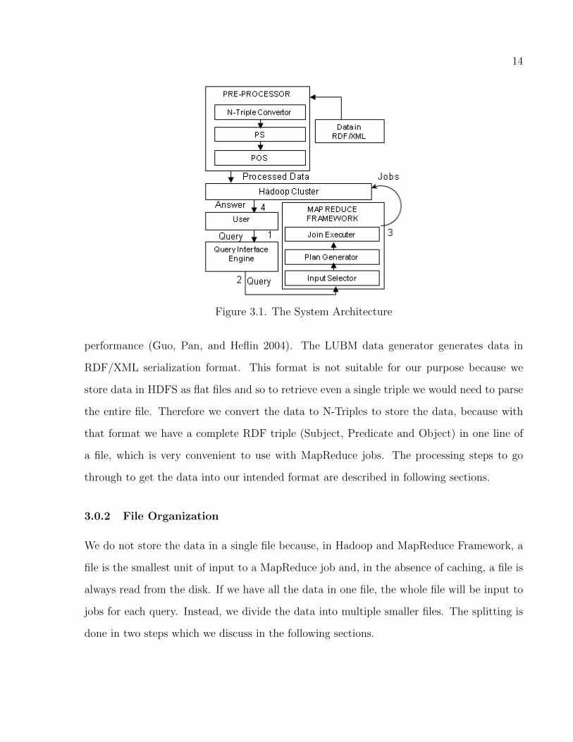
This chapter describes the architecture of our framework. Our framework consists of
two components. The upper part of Figure 3.1 depicts the data preprocessing component
and the lower part shows the query answering one.
We have three subcomponents for data generation and preprocessing. We convert
RDF/XML† to N-Triples† serialization format using our N-Triples Converter component.
The PS component takes the N-Triples data and splits it into predicate files. The predicate
files are then fed into the POS component which splits the predicate files into smaller files
based on the type of objects. These steps are described in Section 3.0.2, 3.0.3 and 3.0.4.
Our MapReduce framework has three sub-components in it. It takes the SPARQL
query from the user and passes it to the Input Selector (see Section 4.2) and Plan Gener-
ator. This component selects the input files, by using our algorithm described in Section
4.3.5, decides how many MapReduce jobs are needed and passes the information to the Join
Executer component which runs the jobs using MapReduce framework. It then relays the
query answer from Hadoop to the user.
3.0.1 Data Generation and Storage
For our experiments, we use the LUBM (Guo, Pan, and Heflin 2005) data set. It is a
benchmark data set designed to enable researchers to evaluate a semantic web repository’s
†http://www.w3.org/TR/rdf-syntax-grammar†http://www.w3.org/2001/sw/RDFCore/ntriples
13
14
Figure 3.1. The System Architecture
performance (Guo, Pan, and Heflin 2004). The LUBM data generator generates data in
RDF/XML serialization format. This format is not suitable for our purpose because we
store data in HDFS as flat files and so to retrieve even a single triple we would need to parse
the entire file. Therefore we convert the data to N-Triples to store the data, because with
that format we have a complete RDF triple (Subject, Predicate and Object) in one line of
a file, which is very convenient to use with MapReduce jobs. The processing steps to go
through to get the data into our intended format are described in following sections.
3.0.2 File Organization
We do not store the data in a single file because, in Hadoop and MapReduce Framework, a
file is the smallest unit of input to a MapReduce job and, in the absence of caching, a file is
always read from the disk. If we have all the data in one file, the whole file will be input to
jobs for each query. Instead, we divide the data into multiple smaller files. The splitting is
done in two steps which we discuss in the following sections.
15
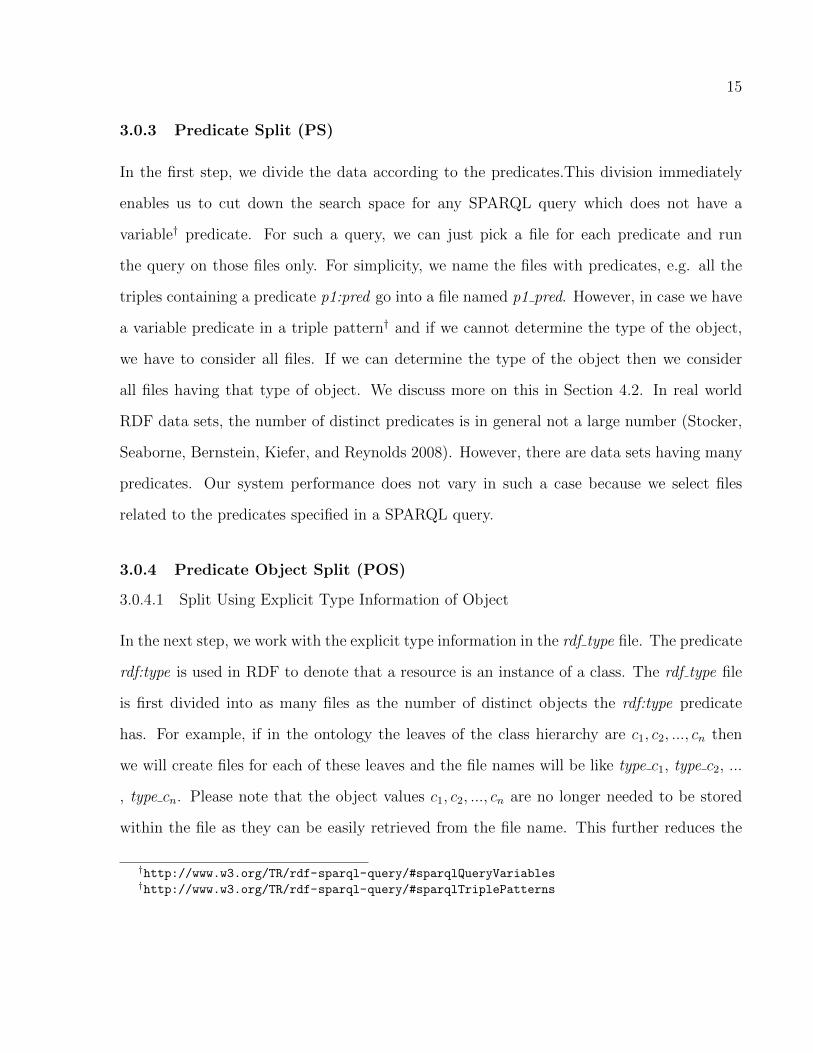
3.0.3 Predicate Split (PS)
In the first step, we divide the data according to the predicates.This division immediately
enables us to cut down the search space for any SPARQL query which does not have a
variable† predicate. For such a query, we can just pick a file for each predicate and run
the query on those files only. For simplicity, we name the files with predicates, e.g. all the
triples containing a predicate p1:pred go into a file named p1 pred. However, in case we have
a variable predicate in a triple pattern† and if we cannot determine the type of the object,
we have to consider all files. If we can determine the type of the object then we consider
all files having that type of object. We discuss more on this in Section 4.2. In real world
RDF data sets, the number of distinct predicates is in general not a large number (Stocker,
Seaborne, Bernstein, Kiefer, and Reynolds 2008). However, there are data sets having many
predicates. Our system performance does not vary in such a case because we select files
related to the predicates specified in a SPARQL query.
3.0.4 Predicate Object Split (POS)
3.0.4.1 Split Using Explicit Type Information of Object
In the next step, we work with the explicit type information in the rdf type file. The predicate
rdf:type is used in RDF to denote that a resource is an instance of a class. The rdf type file
is first divided into as many files as the number of distinct objects the rdf:type predicate
has. For example, if in the ontology the leaves of the class hierarchy are c1, c2, ..., cn then
we will create files for each of these leaves and the file names will be like type c1, type c2, ...
, type cn. Please note that the object values c1, c2, ..., cn are no longer needed to be stored
within the file as they can be easily retrieved from the file name. This further reduces the
†http://www.w3.org/TR/rdf-sparql-query/#sparqlQueryVariables†http://www.w3.org/TR/rdf-sparql-query/#sparqlTriplePatterns
16
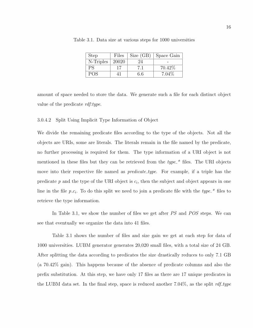
Table 3.1. Data size at various steps for 1000 universities
Step Files Size (GB) Space GainN-Triples 20020 24 -PS 17 7.1 70.42%POS 41 6.6 7.04%
amount of space needed to store the data. We generate such a file for each distinct object
value of the predicate rdf:type.
3.0.4.2 Split Using Implicit Type Information of Object
We divide the remaining predicate files according to the type of the objects. Not all the
objects are URIs, some are literals. The literals remain in the file named by the predicate,
no further processing is required for them. The type information of a URI object is not
mentioned in these files but they can be retrieved from the type * files. The URI objects
move into their respective file named as predicate type. For example, if a triple has the
predicate p and the type of the URI object is ci, then the subject and object appears in one
line in the file p ci. To do this split we need to join a predicate file with the type * files to
retrieve the type information.
In Table 3.1, we show the number of files we get after PS and POS steps. We can
see that eventually we organize the data into 41 files.
Table 3.1 shows the number of files and size gain we get at each step for data of
1000 universities. LUBM generator generates 20,020 small files, with a total size of 24 GB.
After splitting the data according to predicates the size drastically reduces to only 7.1 GB
(a 70.42% gain). This happens because of the absence of predicate columns and also the
prefix substitution. At this step, we have only 17 files as there are 17 unique predicates in
the LUBM data set. In the final step, space is reduced another 7.04%, as the split rdf type
17
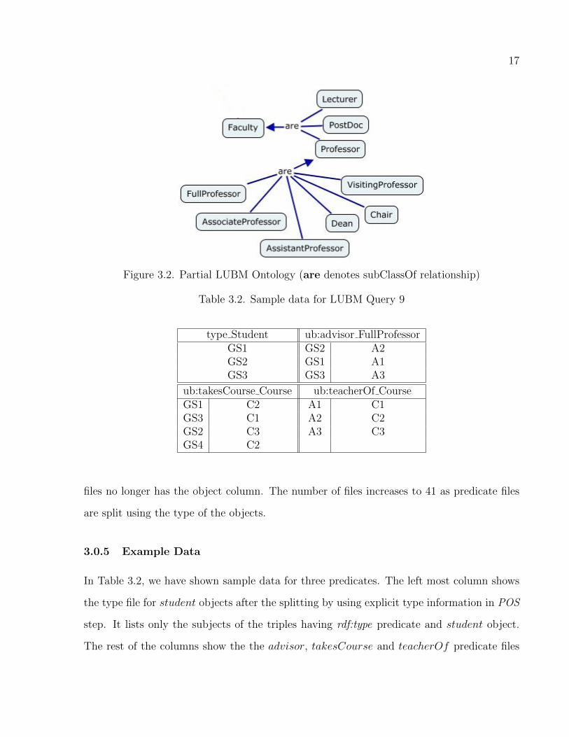
Figure 3.2. Partial LUBM Ontology (are denotes subClassOf relationship)
Table 3.2. Sample data for LUBM Query 9
type Student ub:advisor FullProfessorGS1 GS2 A2GS2 GS1 A1GS3 GS3 A3
ub:takesCourse Course ub:teacherOf CourseGS1 C2 A1 C1GS3 C1 A2 C2GS2 C3 A3 C3GS4 C2
files no longer has the object column. The number of files increases to 41 as predicate files
are split using the type of the objects.
3.0.5 Example Data
In Table 3.2, we have shown sample data for three predicates. The left most column shows
the type file for student objects after the splitting by using explicit type information in POS
step. It lists only the subjects of the triples having rdf:type predicate and student object.
The rest of the columns show the the advisor, takesCourse and teacherOf predicate files
18
after the splitting by using implicit type information in POS step. The prefix ub: stands
for http://www.lehigh.edu/~zhp2/2004/0401/univ-bench.owl#. Each row has a pair of
subject and object. In all cases, the predicate can be retrieved from the filename.
3.0.6 Binary Format
Up to this point, we have shown our files in text format. Text format is the natively supported
format by Hadoop. However, for increased efficiency, storing data in binary format is an
option. We do dictionary encoding to encode the strings with a long value (64-bit). In
this way, we are able to store up to 264 unique strings. We dictionary encode the data using
Hadoop jobs. There are a number of data structures discussed in (Heinz, Zobel, and Williams
2002; Zobel, Heinz, and Williams 2001) to be used to do dictionary encoding. However, these
are not usable in a distributed MapReduce environment. Therefore, we build a prefix tree in
each reducer and generate a unique id for a string by using the reducer id, which is unique
across the job. We generate the dictionary in one job and then run three jobs to replace
the subject, predicate and object of a triple with their corresponding id as text. In the
final job, we convert the triples consisting of ids in text to binary data. Hadoop framework
provides reference implementation for InputFormatter and OutputFormatter classes for text
data. These are the classes used by a Hadoop job to read input for the Map phase and write
output of the Reduce phase. However, because the binary format is a custom one, we have
implemented custom InputFormatter and OutputFormatter classes.
CHAPTER 4
MAP-REDUCE FRAMEWORK
We discuss how we answer SPARQL queries in our MapReduce framework component
in this chapter. In Hadoop, more than one job may be needed to answer a SPARQL query.
Hadoop runs its map and reduce processes in isolation i.e. no two map or reduce process
communicate to each other even though they may be running at the same time. This may
prevent one job to do all the joins necessary to answer a query as sometimes processing
depends on the outcome of some other processing on the same or different piece of data.
With absence of any interprocess communication for map and reduce processes, this is not
possible in Hadoop. Hence, depending on the query, we may need multiple jobs.
The chapter is organized as follows: Section 4.1 presents our query rewriting algorithm
which leverages our schema discussed in Chapter 3 to rewrite queries to their equivalent
simpler forms. Section 4.2 discusses our algorithm to select input files for answering the query.
Section 4.3 talks about cost estimation needed to generate a plan to answer a SPARQL query.
It introduces few terms which we use in the following discussions. Section 4.3.1 discusses
the ideal model we should follow to estimate the cost of a plan. Section 4.3.3 introduces
the heuristics based model we use in practice. Section 4.3.5 presents our heuristics based
greedy algorithm to generate a query plan which uses the cost model introduced in Section
4.3.3. We face tie situations in order to generate a plan in some cases and Section 4.3.6 talks
about how we handle these special cases. Section 4.4 shows how we use the algorithms as
a sub-routine to generate plans for complex queries having OPTIONAL blocks. Section 4.5
19
20
shows how we implement a join in a Hadoop MapReduce job by working through an example
query.
4.1 Query Rewriting
When a query is submitted by the user, we sometimes can take advantage of our schema
and rewrite the query in equivalent simpler form. If a variable has its type information in a
triple pattern having that variable as the subject, the predicate rdf:type and a bound object,
which is the type of the variable, we can eliminate this triple pattern if the variable is used
as an object in some other triple pattern. We can do this because, as described earlier, we
divide the predicate files according to the type of the objects. So if, for the triple pattern
which has the variable as object, we choose the predicate file having that specific type of
objects as input, we do not need the triple pattern having the type information.
An example illustrates it better. Listing 4.1 shows LUBM query 2 and Listing 4.2
shows its rewritten form. Both the variables Y and Z have type information in the sec-
ond and third triple patterns. They are also used as objects in the last three triple pat-
terns. If we include the files ub:memberOf Department, ub:subOrganizationOf University
and ub:undergraduateDegreeFrom University in the input file set for the last triple patterns
respectively, we can guarantee that the values bound to the variables Y and Z in the query
result would be of type ub:University and ub:Department respectively. This is possible be-
cause of the way we divide our data (see Section 3.0.4). The rewritten query has two less
triple patterns. As a result, it got rid of two joins on the variable Y and two on the variable
Z. This rewritten query runs significantly faster than the original query because of having
four less joins. Here the rewritten query has predicates which serve as a filename for our
input selection phase described in Section 4.2. Note that this type of rewriting is possible
even if there is no ontology associated with the dataset. This type of rewriting is very useful
because we observed that most of the SPARQL queries have triple patterns with rdf:type
21
predicates describing the type of a variable. For example, all the queries of LUBM dataset
and all but two queries of SP2B dataset have at least one such triple pattern.
Algorithm 1 RewriteQuery(Query q)
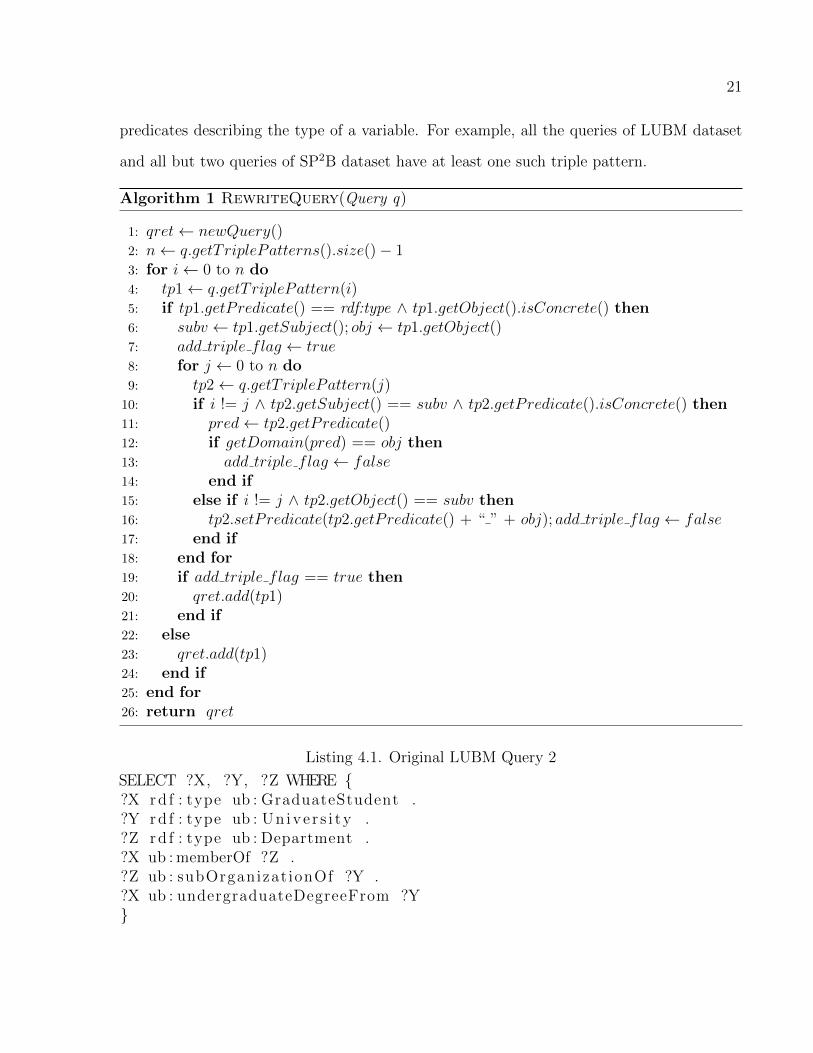
1: qret← newQuery()2: n← q.getTriplePatterns().size()− 13: for i← 0 to n do4: tp1← q.getTriplePattern(i)5: if tp1.getPredicate() == rdf:type ∧ tp1.getObject().isConcrete() then6: subv ← tp1.getSubject(); obj ← tp1.getObject()7: add triple flag ← true8: for j ← 0 to n do9: tp2← q.getTriplePattern(j)10: if i != j ∧ tp2.getSubject() == subv ∧ tp2.getPredicate().isConcrete() then11: pred← tp2.getPredicate()12: if getDomain(pred) == obj then13: add triple flag ← false14: end if15: else if i != j ∧ tp2.getObject() == subv then16: tp2.setPredicate(tp2.getPredicate() + “ ” + obj); add triple flag ← false17: end if18: end for19: if add triple flag == true then20: qret.add(tp1)21: end if22: else23: qret.add(tp1)24: end if25: end for26: return qret
Listing 4.1. Original LUBM Query 2
SELECT ?X, ?Y, ?Z WHERE {?X rd f : type ub : GraduateStudent .?Y rd f : type ub : Un ive r s i ty .?Z rd f : type ub : Department .?X ub : memberOf ?Z .?Z ub : subOrganizat ionOf ?Y .?X ub : undergraduateDegreeFrom ?Y}
22
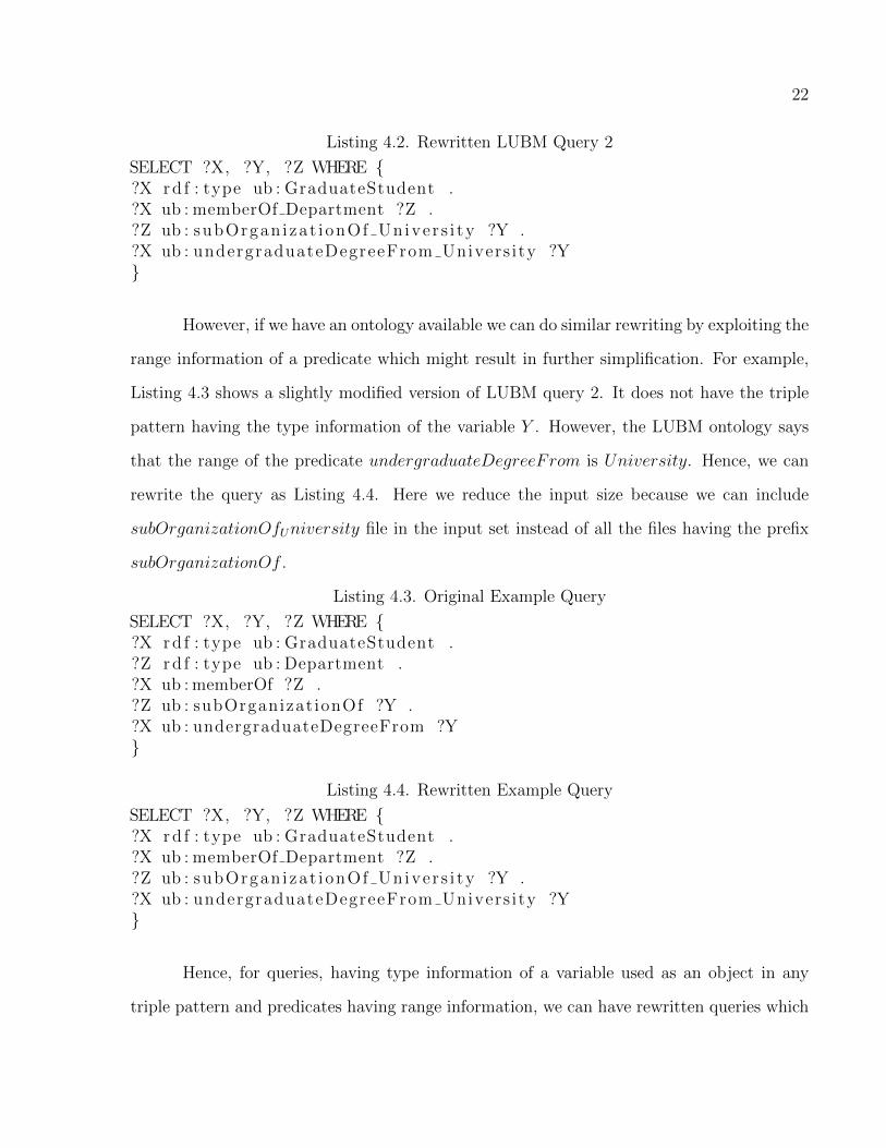
Listing 4.2. Rewritten LUBM Query 2
SELECT ?X, ?Y, ?Z WHERE {?X rd f : type ub : GraduateStudent .?X ub : memberOf Department ?Z .?Z ub : subOrgan izat ionOf Univer s i ty ?Y .?X ub : undergraduateDegreeFrom Univers ity ?Y}
However, if we have an ontology available we can do similar rewriting by exploiting the
range information of a predicate which might result in further simplification. For example,
Listing 4.3 shows a slightly modified version of LUBM query 2. It does not have the triple
pattern having the type information of the variable Y . However, the LUBM ontology says
that the range of the predicate undergraduateDegreeFrom is University. Hence, we can
rewrite the query as Listing 4.4. Here we reduce the input size because we can include
subOrganizationOfUniversity file in the input set instead of all the files having the prefix
subOrganizationOf .
Listing 4.3. Original Example Query
SELECT ?X, ?Y, ?Z WHERE {?X rd f : type ub : GraduateStudent .?Z rd f : type ub : Department .?X ub : memberOf ?Z .?Z ub : subOrganizat ionOf ?Y .?X ub : undergraduateDegreeFrom ?Y}
Listing 4.4. Rewritten Example Query
SELECT ?X, ?Y, ?Z WHERE {?X rd f : type ub : GraduateStudent .?X ub : memberOf Department ?Z .?Z ub : subOrgan izat ionOf Univer s i ty ?Y .?X ub : undergraduateDegreeFrom Univers ity ?Y}
Hence, for queries, having type information of a variable used as an object in any
triple pattern and predicates having range information, we can have rewritten queries which
23
reduces input size and may eliminate few joins. Both of these have significant impact on
query runtime.
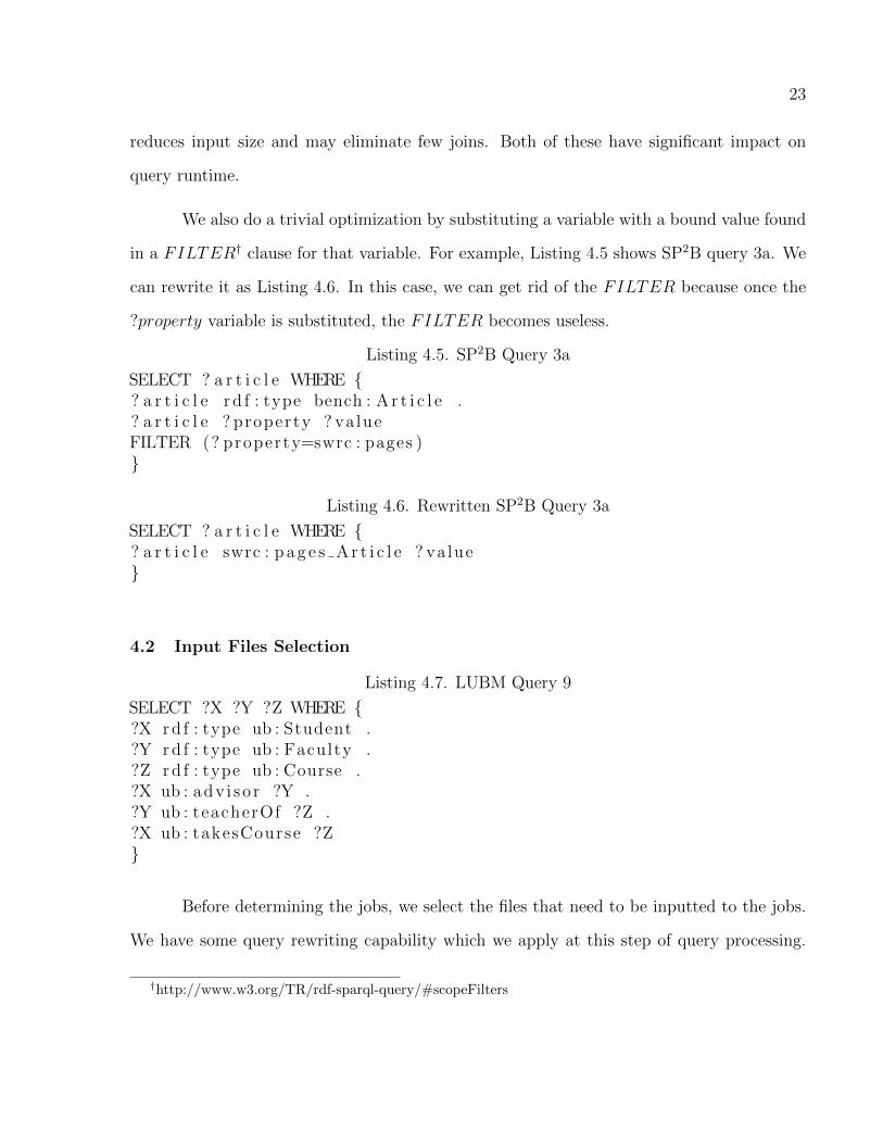
We also do a trivial optimization by substituting a variable with a bound value found
in a FILTER† clause for that variable. For example, Listing 4.5 shows SP2B query 3a. We
can rewrite it as Listing 4.6. In this case, we can get rid of the FILTER because once the
?property variable is substituted, the FILTER becomes useless.
Listing 4.5. SP2B Query 3a
SELECT ? a r t i c l e WHERE {? a r t i c l e rd f : type bench : A r t i c l e .? a r t i c l e ? property ? valueFILTER (? property=swrc : pages )}
Listing 4.6. Rewritten SP2B Query 3a
SELECT ? a r t i c l e WHERE {? a r t i c l e swrc : p a g e s A r t i c l e ? va lue}
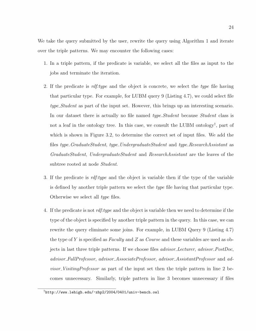
4.2 Input Files Selection
Listing 4.7. LUBM Query 9
SELECT ?X ?Y ?Z WHERE {?X rd f : type ub : Student .?Y rd f : type ub : Faculty .?Z rd f : type ub : Course .?X ub : adv i so r ?Y .?Y ub : teacherOf ?Z .?X ub : takesCourse ?Z}
Before determining the jobs, we select the files that need to be inputted to the jobs.
We have some query rewriting capability which we apply at this step of query processing.
†http://www.w3.org/TR/rdf-sparql-query/#scopeFilters
24
We take the query submitted by the user, rewrite the query using Algorithm 1 and iterate
over the triple patterns. We may encounter the following cases:
1. In a triple pattern, if the predicate is variable, we select all the files as input to the
jobs and terminate the iteration.
2. If the predicate is rdf:type and the object is concrete, we select the type file having
that particular type. For example, for LUBM query 9 (Listing 4.7), we could select file
type Student as part of the input set. However, this brings up an interesting scenario.
In our dataset there is actually no file named type Student because Student class is
not a leaf in the ontology tree. In this case, we consult the LUBM ontology†, part of
which is shown in Figure 3.2, to determine the correct set of input files. We add the
files type GraduateStudent, type UndergraduateStudent and type ResearchAssistant as
GraduateStudent, UndergraduateStudent and ResearchAssistant are the leaves of the
subtree rooted at node Student.
3. If the predicate is rdf:type and the object is variable then if the type of the variable
is defined by another triple pattern we select the type file having that particular type.
Otherwise we select all type files.
4. If the predicate is not rdf:type and the object is variable then we need to determine if the
type of the object is specified by another triple pattern in the query. In this case, we can
rewrite the query eliminate some joins. For example, in LUBM Query 9 (Listing 4.7)
the type of Y is specified as Faculty and Z as Course and these variables are used as ob-
jects in last three triple patterns. If we choose files advisor Lecturer, advisor PostDoc,
advisor FullProfessor, advisor AssociateProfessor, advisor AssistantProfessor and ad-
visor VisitingProfessor as part of the input set then the triple pattern in line 2 be-
comes unnecessary. Similarly, triple pattern in line 3 becomes unnecessary if files
†http://www.lehigh.edu/~zhp2/2004/0401/univ-bench.owl
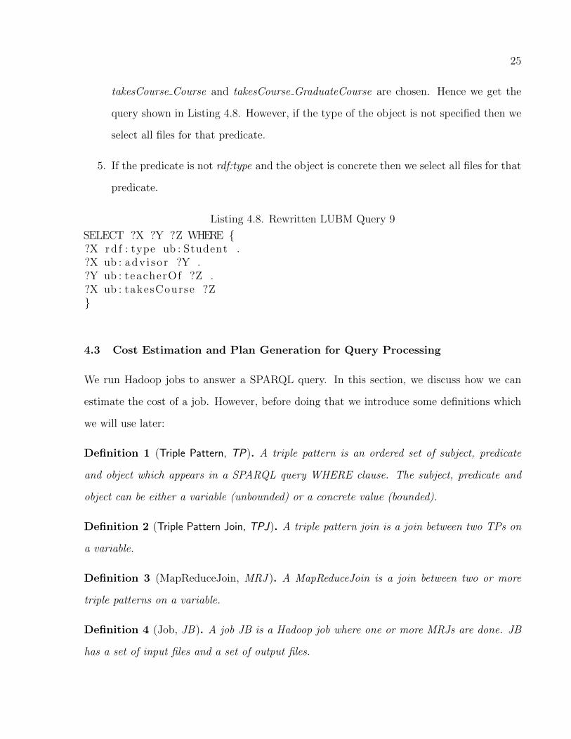
25
takesCourse Course and takesCourse GraduateCourse are chosen. Hence we get the
query shown in Listing 4.8. However, if the type of the object is not specified then we
select all files for that predicate.
5. If the predicate is not rdf:type and the object is concrete then we select all files for that
predicate.
Listing 4.8. Rewritten LUBM Query 9
SELECT ?X ?Y ?Z WHERE {?X rd f : type ub : Student .?X ub : adv i so r ?Y .?Y ub : teacherOf ?Z .?X ub : takesCourse ?Z}
4.3 Cost Estimation and Plan Generation for Query Processing
We run Hadoop jobs to answer a SPARQL query. In this section, we discuss how we can
estimate the cost of a job. However, before doing that we introduce some definitions which
we will use later:
Definition 1 (Triple Pattern, TP). A triple pattern is an ordered set of subject, predicate
and object which appears in a SPARQL query WHERE clause. The subject, predicate and
object can be either a variable (unbounded) or a concrete value (bounded).
Definition 2 (Triple Pattern Join, TPJ). A triple pattern join is a join between two TPs on
a variable.
Definition 3 (MapReduceJoin, MRJ ). A MapReduceJoin is a join between two or more
triple patterns on a variable.
Definition 4 (Job, JB). A job JB is a Hadoop job where one or more MRJs are done. JB
has a set of input files and a set of output files.

26
Figure 4.1. NCMRJ and CMRJ Example
Definition 5 (Conflicting MapReduceJoins, CMRJ ). Conflicting MapReduceJoins is a pair
of MRJs on different variables sharing a triple pattern.
Definition 6 (Non-Conflicting MapReduceJoins, NCMRJ ). Non-conflicting MapReduce-
Joins is a pair of MRJs either not sharing any triple pattern or sharing a triple pattern and
the MRJs are on same variable.
Listing 4.9. LUBM Query 12
SELECT ?X WHERE {?X rd f : type ub : Chair .?Y rd f : type ub : Department .?X ub : worksFor ?Y .?Y ub : subOrganizat ionOf <http ://www. Un ive r s i ty0 . edu>}
An example will illustrate these terms better. In Listing 4.9, we show LUBM Query
12. Lines 2, 3, 4 and 5 each have a triple pattern. The join between TPs in lines 2 and 4 on
variable ?X is an MRJ. If we do two MRJs, one between TPs in lines 2 and 4 on variable
?X and the other between TPs in lines 4 and 5 on variable ?Y , there will be a CMRJ as TP
in line 4 (?X ub:worksFor ?Y ) takes part in two MRJs on two different variables
?X and ?Y . This is shown on the right in Figure 4.1. This type of join is called CMRJ
because in a Hadoop job more than one variable of a TP cannot be a key at the same time
and MRJs are performed on keys. A NCMRJ, shown on the left in Figure 4.1, would be
27
one MRJ between triple patterns in lines 2 and 4 on variable ?X and another MRJ between
triple patterns in lines 3 and 5 on variable ?Y . These two MRJs can make up a JB.
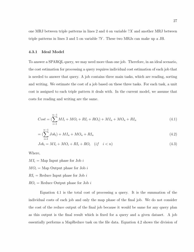
4.3.1 Ideal Model
To answer a SPARQL query, we may need more than one job. Therefore, in an ideal scenario,
the cost estimation for processing a query requires individual cost estimation of each job that
is needed to answer that query. A job contains three main tasks, which are reading, sorting
and writing. We estimate the cost of a job based on these three tasks. For each task, a unit
cost is assigned to each triple pattern it deals with. In the current model, we assume that
costs for reading and writing are the same.
Cost = (n−1∑i=1
MIi +MOi +RIi +ROi) +MIn +MOn +RIn (4.1)
= (n−1∑i=1
Jobi) +MIn +MOn +RIn (4.2)
Jobi = MIi +MOi +RIi +ROi (if i < n) (4.3)
Where,
MIi = Map Input phase for Job i
MOi = Map Output phase for Job i
RIi = Reduce Input phase for Job i
ROi = Reduce Output phase for Job i
Equation 4.1 is the total cost of processing a query. It is the summation of the
individual costs of each job and only the map phase of the final job. We do not consider
the cost of the reduce output of the final job because it would be same for any query plan
as this output is the final result which is fixed for a query and a given dataset. A job
essentially performs a MapReduce task on the file data. Equation 4.2 shows the division of
28
the MapReduce task into subtasks. Hence, to estimate the cost of each job, we will combine
the estimated cost of each subtask.
Map Input (MI) phase: This phase reads the triple patterns from the selected
input files stored in the HDFS. Therefore, we can estimate the cost for the MI phase to be
equal to the total number of triples in each of the selected files.
Map Output Phase (MO): The estimation of the MO phase depends on the type
of query being processed. If the query has no bound variable (e.g. [?X ub:worksFor ?Y]),
then the output of the Map phase is equal to the input. All of the triple patterns are
transformed into key-value pairs and given as output. Therefore, for such a query the MO
cost will be the same as MI cost. However, if the query involves a bound variable, (e.g. [?Y
ub:subOrganizationOf <http://www.U0.edu>]), then, before making the key-value pairs, a
bound component selectivity estimation can be applied. The resulting estimate for the triple
patterns will account for the cost of Map Output phase. The selected triples are written to
a local disk.
Reduce Input Phase (RI): In this phase, the triples from the Map output phase
are read via HTTP and then sorted based on their key values. After sorting, the triples
with identical keys are grouped together. Therefore, the cost estimation for the RI phase is
equal to the MO phase. The number of key-value pairs that are sorted in RI is equal to the
number of key-value pairs generated in the MO phase.
Reduce Output Phase (RO): The RO phase deals with performing the joins.
Therefore, it is in this phase we can use the join triple pattern selectivity summary statistics
to estimate the size of its output. Section 4.3.3 talks in details about the join triple pattern
selectivity summary statistics needed for our framework.
However, in practice, the above discussion is applicable for the first job only. For the
subsequent jobs, we lack both the precise knowledge and estimate of the number of triple
29
patterns selected after applying the join in the first job. Therefore, for these jobs, we can
take the size of the RO phase of the first job as an upper bound on the different phases of
the subsequent jobs.
Equation 4.3 shows a very important postulation. It illustrates the total cost of an
intermediate job, when i < n, includes the cost of the RO phase in calculating the total cost
of the job.
4.3.2 The GenerateBestPlan Algorithm
In this section, we present our new algorithm GenerateBestPlan (Algorithm 2) which based
on the cost model described in section 4.3 provides the best query execution plan for a query.
It uses the two coloring scheme to generate all possible plans and calculates cost for each
of them as it generates them. It returns the best plan i.e. the plan with the minimum cost
when it is finished. As map and reduce processes in Hadoop jobs do not have interprocess
communication, joins which depend on each other can not be done all at once. The two
coloring scheme nicely represent this scenario where adjacent nodes of a graph cannot have
same color. We use a certain color for a node, which represents a join, signifying that the join
is chosen. Edges are drawn between dependent joins hence an adjacent node representing a
dependent join cannot have the same color and the join is not selected with its depend join.
We chose the scheme as it perfectly meets our need in this way.
For a query Q we build a graph G = (V,E) where V is the set of vertices and E is the
set of edges. For each triple pattern in the query Q we build a vertex v which makes up the
set V . Hence |V | is equal to the number of triple patterns in Q. We put an edge e between
vi and vj, where i 6= j, if and only if their corresponding triple patterns share at least one
variable. We label the edge e with all the variable names that were shared between vi and
vj. These edges make up the set E. Each edge represents as many joins as the number of
variables it has in its label. Hence, total number of joins present in the graph is the total
30
number of variables mentioned in the labels of all edges. An example illustrates it better.
We have chosen LUBM (Guo, Pan, and Heflin 2005) query 12 for that purpose. Listing 4.9
shows the query.
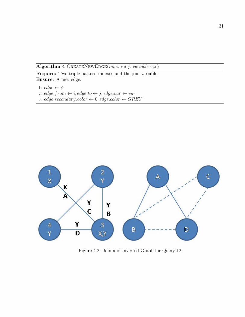
The graph we build at first for the query is shown in figure 4.2. The nodes are
numbered in the order they appear in the query.
Algorithm 2 GenerateBestPlan(Query q)
Require: A Query object returned by RewriteQuery algorithm.Ensure: The number of jobs and their details needed to answer the query.
1: plans← CreateEmptyPriorityQueue()2: jg ← CreateJoinGraph(q)3: ig ← CreateInvertedGraph(jg)4: jobs← φ5: ColorGraph1(jg, ig, 0, jobs)6: return getHeadFromPriorityQueue(plans)
Algorithm 3 CreateJoinGraph(Query q)
Require: A Query object.Ensure: A join graph based on a query
1: tp← getTriplePatterns(q)2: JoinGraph← φ3: edges← φ4: for i← 0 to |tp| do5: for j ← i+ 1 to |tp| do6: if (var ← sharesV ariable(tp[i], tp[j])) != φ then7: edges← edges ∪ CreateNewEdge(i, j, var)8: end if9: end for10: end for11: JoinGraph.edges← edges12: return JoinGraph
In the left graph of figure 4.2, each node in the figure has a node number in the first
line and variables it has in the following line. Nodes 1 and 3 share the variable X hence
31
Algorithm 4 CreateNewEdge(int i, int j, variable var)
Require: Two triple pattern indexes and the join variable.Ensure: A new edge.
1: edge← φ2: edge.from← i; edge.to← j; edge.var ← var3: edge.secondary color ← 0; edge.color ← GREY
Figure 4.2. Join and Inverted Graph for Query 12
32
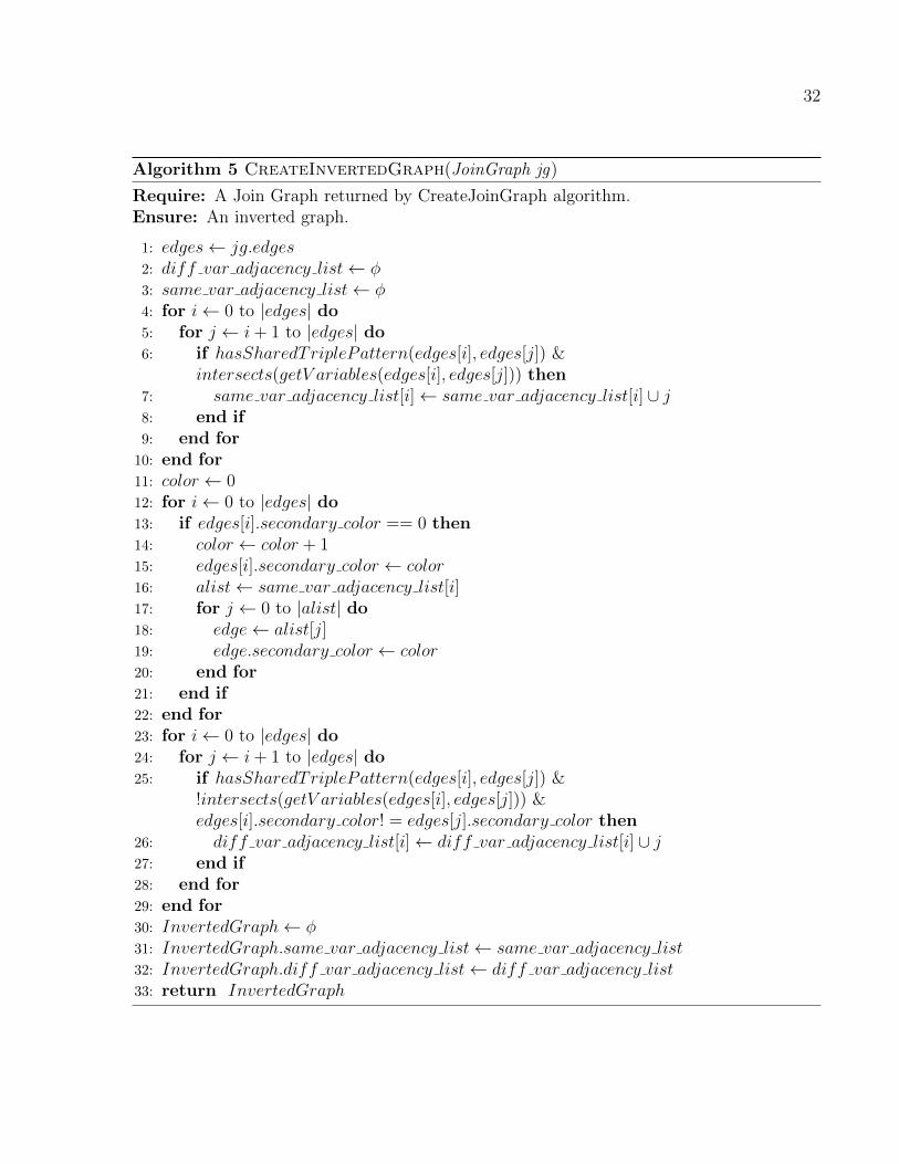
Algorithm 5 CreateInvertedGraph(JoinGraph jg)
Require: A Join Graph returned by CreateJoinGraph algorithm.Ensure: An inverted graph.
1: edges← jg.edges2: diff var adjacency list← φ3: same var adjacency list← φ4: for i← 0 to |edges| do5: for j ← i+ 1 to |edges| do6: if hasSharedTriplePattern(edges[i], edges[j]) &
intersects(getV ariables(edges[i], edges[j])) then7: same var adjacency list[i]← same var adjacency list[i] ∪ j8: end if9: end for10: end for11: color ← 012: for i← 0 to |edges| do13: if edges[i].secondary color == 0 then14: color ← color + 115: edges[i].secondary color ← color16: alist← same var adjacency list[i]17: for j ← 0 to |alist| do18: edge← alist[j]19: edge.secondary color ← color20: end for21: end if22: end for23: for i← 0 to |edges| do24: for j ← i+ 1 to |edges| do25: if hasSharedTriplePattern(edges[i], edges[j]) &
!intersects(getV ariables(edges[i], edges[j])) &edges[i].secondary color! = edges[j].secondary color then
26: diff var adjacency list[i]← diff var adjacency list[i] ∪ j27: end if28: end for29: end for30: InvertedGraph← φ31: InvertedGraph.same var adjacency list← same var adjacency list32: InvertedGraph.diff var adjacency list← diff var adjacency list33: return InvertedGraph
33
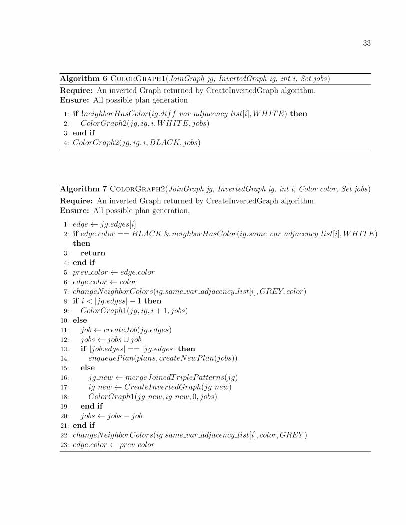
Algorithm 6 ColorGraph1(JoinGraph jg, InvertedGraph ig, int i, Set jobs)
Require: An inverted Graph returned by CreateInvertedGraph algorithm.Ensure: All possible plan generation.
1: if !neighborHasColor(ig.diff var adjacency list[i],WHITE) then2: ColorGraph2(jg, ig, i,WHITE, jobs)3: end if4: ColorGraph2(jg, ig, i, BLACK, jobs)
Algorithm 7 ColorGraph2(JoinGraph jg, InvertedGraph ig, int i, Color color, Set jobs)
Require: An inverted Graph returned by CreateInvertedGraph algorithm.Ensure: All possible plan generation.
1: edge← jg.edges[i]2: if edge.color == BLACK & neighborHasColor(ig.same var adjacency list[i],WHITE)
then3: return4: end if5: prev color ← edge.color6: edge.color ← color7: changeNeighborColors(ig.same var adjacency list[i], GREY, color)8: if i < |jg.edges| − 1 then9: ColorGraph1(jg, ig, i+ 1, jobs)10: else11: job← createJob(jg.edges)12: jobs← jobs ∪ job13: if |job.edges| == |jg.edges| then14: enqueueP lan(plans, createNewPlan(jobs))15: else16: jg new ← mergeJoinedTriplePatterns(jg)17: ig new ← CreateInvertedGraph(jg new)18: ColorGraph1(jg new, ig new, 0, jobs)19: end if20: jobs← jobs− job21: end if22: changeNeighborColors(ig.same var adjacency list[i], color,GREY )23: edge.color ← prev color

34
there is an edge between them having the label X. Similarly, nodes 2, 3 and 4 have edges
between them because they share the variable Y . The graph has total 4 joins.
Algorithm 2 makes use of another graph built from G. We build graph G′ =
(V ′, E1, E2) where for each e ∈ E we have a v ∈ V ′ i.e. all the edges of graph G be-
come nodes in graph G′. Hence |V ′| is equal to the number of triple pattern joins in Q. Each
of the nodes v ∈ V ′ is accessible by an integer index. We put an edge e1 ∈ E1 between vi
and vj, where i 6= j, if and only if their corresponding edges ei ∈ E and ej ∈ E share a node
v ∈ V and there is at least one shared join variable. Similarly, We put an edge e2 ∈ E1
between vi and vj, where i 6= j, if and only if their corresponding edges ei ∈ E and ej ∈ E
share a node v ∈ V and there is no shared join variable. We call the graph G′ the inverted
graph of G. We call the edges of E1 dashed edges and E2 solid edges. In figure 4.2, we see
the inverted graph of query 12 on the right. The nodes A, B, C and D in the graph are the
edges of the join graph on the right. A has two solid edges with B and D as it shares node in
join graph with those joins but does not share any variable. B, C and D have dashed edges
between them as they share both nodes and variables.
In short, our GenerateBestPlan algorithm maintains a priority queue which holds
query processing plans. Priority is determined by the cost of a plan. It then creates a join
graph G for a query Q and an inverted graph G′ from G. It then calls ColorGraph1 algorithm
to color the inverted graph and generate plans.
Algorithm 2 shows the pseudocode of the GenerateBestPlan algorithm. In line 1,
it creates an empty priority queue which holds all the plans eventually. The priority is
determined by the cost of a plan. The lower the cost the higher the priority. In line 2, it
calls the routine CreateJoinGraph, described in algorithm 3, which returns graph G. In line
3, it calls the routine CreateInvertedGraph, described in algorithm 5, which returns graph
G′. In line 4, it initializes an empty set of Hadoop jobs jobs. In line 5, a recursive routine

35
ColorGraph1, described in algorithm 6, is called with G, G′, jobs and the number 0 which
is the index of the node of V ′.
Algorithm 3 shows how graph G is built. In line 4 - 10, it checks each pair of triple
patterns for shared variables. If such a variable is found it adds an edge e between two nodes
in line 7. It calls the routine CreateNewEdge to create an edge. In line 12 it returns the
constructed graph. Algorithm 4 shows the CreateNewEdge routine. It creates a new edge
and initializes it with node indexes and initial colors. An edge has a color which can be
either grey, white or black. Initially, the color is grey. There is also a secondary color which
can have any value. This color is used to construct the inverted graph. The initial secondary
color is an integer 0.
Algorithm 5 shows how graph G′ is built. First the dashed edges are created. In lines
4 to 10, the algorithm checks if two edges of graph G share a node and also have shared
variable in their labels. If the condition satisfies in line 6, a new dashed edge is added in line
7. It then assigns secondary colors in lines 11 to 22. The color starts from 1. In line 13, it
checks if a node has the initial secondary color 0. In such a case it creates a new secondary
color and assigns it to the node. In lines 16 to 20 it assigns this secondary color to all its
dashed edge neighbors. Then the routine creates the solid edges in lines 23 to 29. In line
25, it checks if two edges of graph G share a node, do not share any shared variable in their
labels and do not have same secondary colors. If the condition satisfies, it adds a new solid
edge to the graph. The purpose of the secondary color is to prevent nodes sharing dashed
edges from having solid edges. We discuss the algorithms for two coloring in the following
section.
4.3.2.1 Two Coloring Scheme
The two-coloring scheme is actually applied to the inverted graph. At first we construct two
graphs G0 and its inverted graph G′0 where 0 means the first join graph. Then we try to color
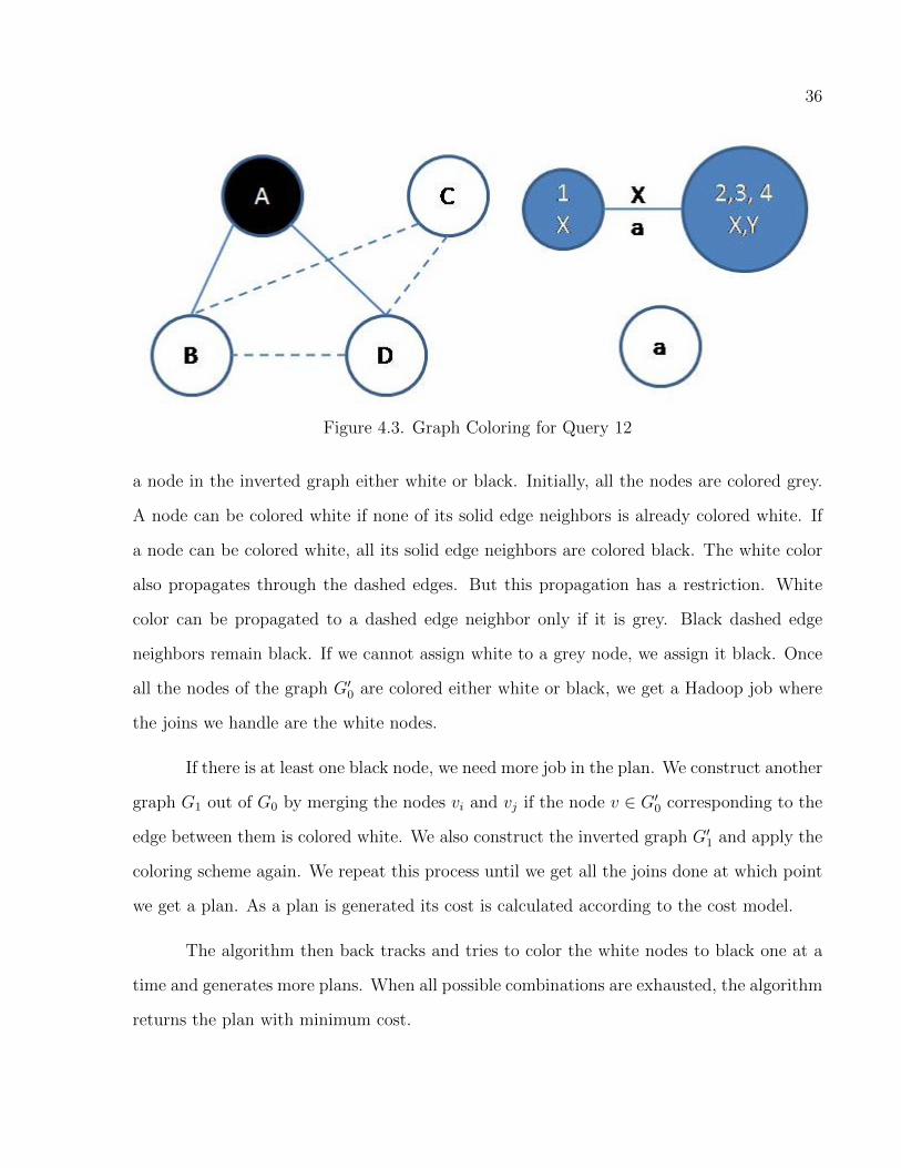
36
Figure 4.3. Graph Coloring for Query 12
a node in the inverted graph either white or black. Initially, all the nodes are colored grey.
A node can be colored white if none of its solid edge neighbors is already colored white. If
a node can be colored white, all its solid edge neighbors are colored black. The white color
also propagates through the dashed edges. But this propagation has a restriction. White
color can be propagated to a dashed edge neighbor only if it is grey. Black dashed edge
neighbors remain black. If we cannot assign white to a grey node, we assign it black. Once
all the nodes of the graph G′0 are colored either white or black, we get a Hadoop job where
the joins we handle are the white nodes.
If there is at least one black node, we need more job in the plan. We construct another
graph G1 out of G0 by merging the nodes vi and vj if the node v ∈ G′0 corresponding to the
edge between them is colored white. We also construct the inverted graph G′1 and apply the
coloring scheme again. We repeat this process until we get all the joins done at which point
we get a plan. As a plan is generated its cost is calculated according to the cost model.
The algorithm then back tracks and tries to color the white nodes to black one at a
time and generates more plans. When all possible combinations are exhausted, the algorithm
returns the plan with minimum cost.
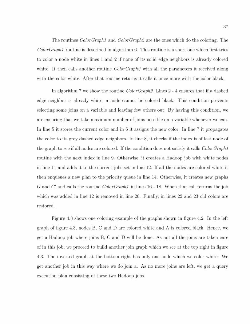
37
The routines ColorGraph1 and ColorGraph2 are the ones which do the coloring. The
ColorGraph1 routine is described in algorithm 6. This routine is a short one which first tries
to color a node white in lines 1 and 2 if none of its solid edge neighbors is already colored
white. It then calls another routine ColorGraph2 with all the parameters it received along
with the color white. After that routine returns it calls it once more with the color black.
In algorithm 7 we show the routine ColorGraph2. Lines 2 - 4 ensures that if a dashed
edge neighbor is already white, a node cannot be colored black. This condition prevents
selecting some joins on a variable and leaving few others out. By having this condition, we
are ensuring that we take maximum number of joins possible on a variable whenever we can.
In line 5 it stores the current color and in 6 it assigns the new color. In line 7 it propagates
the color to its grey dashed edge neighbors. In line 8, it checks if the index is of last node of
the graph to see if all nodes are colored. If the condition does not satisfy it calls ColorGraph1
routine with the next index in line 9. Otherwise, it creates a Hadoop job with white nodes
in line 11 and adds it to the current jobs set in line 12. If all the nodes are colored white it
then enqueues a new plan to the priority queue in line 14. Otherwise, it creates new graphs
G and G′ and calls the routine ColorGraph1 in lines 16 - 18. When that call returns the job
which was added in line 12 is removed in line 20. Finally, in lines 22 and 23 old colors are
restored.
Figure 4.3 shows one coloring example of the graphs shown in figure 4.2. In the left
graph of figure 4.3, nodes B, C and D are colored white and A is colored black. Hence, we
get a Hadoop job where joins B, C and D will be done. As not all the joins are taken care
of in this job, we proceed to build another join graph which we see at the top right in figure
4.3. The inverted graph at the bottom right has only one node which we color white. We
get another job in this way where we do join a. As no more joins are left, we get a query
execution plan consisting of these two Hadoop jobs.
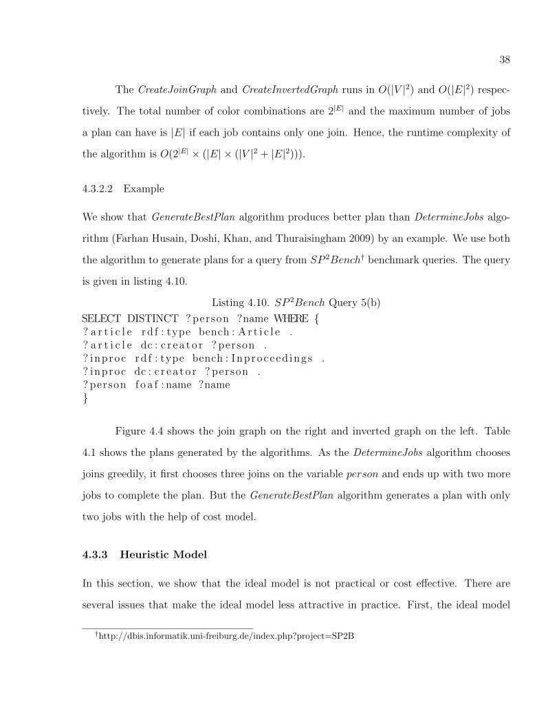
38
The CreateJoinGraph and CreateInvertedGraph runs in O(|V |2) and O(|E|2) respec-
tively. The total number of color combinations are 2|E| and the maximum number of jobs
a plan can have is |E| if each job contains only one join. Hence, the runtime complexity of
the algorithm is O(2|E| × (|E| × (|V |2 + |E|2))).
4.3.2.2 Example
We show that GenerateBestPlan algorithm produces better plan than DetermineJobs algo-
rithm (Farhan Husain, Doshi, Khan, and Thuraisingham 2009) by an example. We use both
the algorithm to generate plans for a query from SP 2Bench† benchmark queries. The query
is given in listing 4.10.
Listing 4.10. SP 2Bench Query 5(b)
SELECT DISTINCT ? person ?name WHERE {? a r t i c l e rd f : type bench : A r t i c l e .? a r t i c l e dc : c r e a t o r ? person .? inproc rd f : type bench : Inproceed ings .? inproc dc : c r e a t o r ? person .? person f o a f : name ?name}
Figure 4.4 shows the join graph on the right and inverted graph on the left. Table
4.1 shows the plans generated by the algorithms. As the DetermineJobs algorithm chooses
joins greedily, it first chooses three joins on the variable person and ends up with two more
jobs to complete the plan. But the GenerateBestPlan algorithm generates a plan with only
two jobs with the help of cost model.
4.3.3 Heuristic Model
In this section, we show that the ideal model is not practical or cost effective. There are
several issues that make the ideal model less attractive in practice. First, the ideal model
†http://dbis.informatik.uni-freiburg.de/index.php?project=SP2B
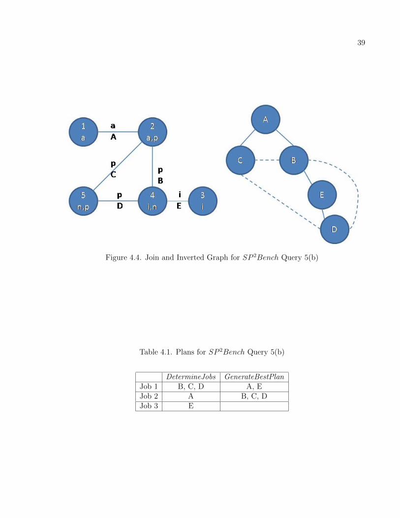
39
Figure 4.4. Join and Inverted Graph for SP 2Bench Query 5(b)
Table 4.1. Plans for SP 2Bench Query 5(b)
DetermineJobs GenerateBestPlanJob 1 B, C, D A, EJob 2 A B, C, DJob 3 E
40
considers simple abstract costs, namely the number of triples read and written by the different
phases ignoring the actual cost of copying, sorting, etc. these triples, and the overhead for
running jobs in Hadoop. But accurately incorporating those costs in the model is a difficult
task. Even making reasonably good estimation may be non-trivial. Second, to estimate
intermediate join outputs, we need to maintain comprehensive summary statistics. In a
MapReduce job in Hadoop, all the joins on a variable are joined together. For example, in
the rewritten LUBM Query 9 (Listing 4.8) there are three joins on variable X. When a job
is run to do the join on X, all the joins on X between triple patterns 1, 2 and 4 are done.
If there were more than 3 joins on X all will still be handled in one job. This shows that in
order to gather summary statistics to estimate join selectivity we face an exponential number
of join cases. For example, between triple patterns having predicates p1, p2 and p3, there may
be 23 types of joins because in each triple pattern, a variable can occur either as a subject or
an object. In the case of the rewritten Query 9, it is a subject-subject-subject join between
1, 2 and 4. There can be more types of join between these three e.g. subject-object-subject,
object-subject-object etc. That means, between P predicates, there can be 2P type of joins
on a single variable (ignoring the possibility that a variable may appear both as a subject
and object in a triple pattern). If there are P predicates in the data set, total number of
cases for which we need to collect summary statistics can be calculated by the formula:
22 × CP2 + 23 × CP
3 + ...+ 2P × CPP
In LUBM data set, there are 17 predicates. So, in total there are 129,140,128 cases
which is a large number. Gathering summary statistics for such a large number of cases
would be very much time and space consuming. Hence, we took an alternate approach.
We observe that there is significant overhead for running a job in Hadoop. Therefore,
if we minimize the number of jobs to answer a query, we get the fastest plan. The overhead
is incurred by several disk I/O and network transfers that are integral part of any Hadoop
41
job. When a job is submitted to Hadoop cluster at least the following set of actions take
place:
1. The Executable file is transferred from client machine to Hadoop JobTracker†,
2. The JobTracker decides which TaskTrackers† will execute the job, 3. The Executable
file is distributed to the TaskTrackers over the network, 4. Map processes start by reading
data from HDFS, 5. Map outputs are written to discs, 6. Map outputs are read from discs,
shuffled (transferred over the network to TaskTrackers which would run Reduce processes),
sorted and written to discs, 7. Reduce processes start by reading the input from the discs,
8. Reduce outputs are written to discs.
These disk operations and network transfers are expensive operations even for a small
amount of data. For example, in our experiments, we observed that the overhead incurred
by one job is almost equivalent to reading a billion triples. The reason is in every job
the output of the map process is always sorted before feeding the reduce processes. This
sorting is unavoidable even if it is not needed by the user. Therefore, it would be less costly
to process several hundred million more triples in n jobs, rather than processing several
hundred million less triples in n + 1 jobs.
Listing 4.11. Experiment Query
?S1 ub : adv i so r ?X .?X ub : headOf ?Z .?Z ub : subOrganizat ionOf ?Y .?S2 ub : mastersDegreeFrom ?Y
To further investigate, we did an experiment where we used the query shown in Listing
4.11. Here the join selectivity between TP 2 and 3 on ?Z is the highest. Hence, a query plan
generation algorithm which uses selectivity factors to pick joins would select this join for the
first job. As the other TPs 1 and 4 share variables with either TP 2 or 3, they cannot take
†http://wiki.apache.org/hadoop/JobTracker†http://wiki.apache.org/hadoop/TaskTracker
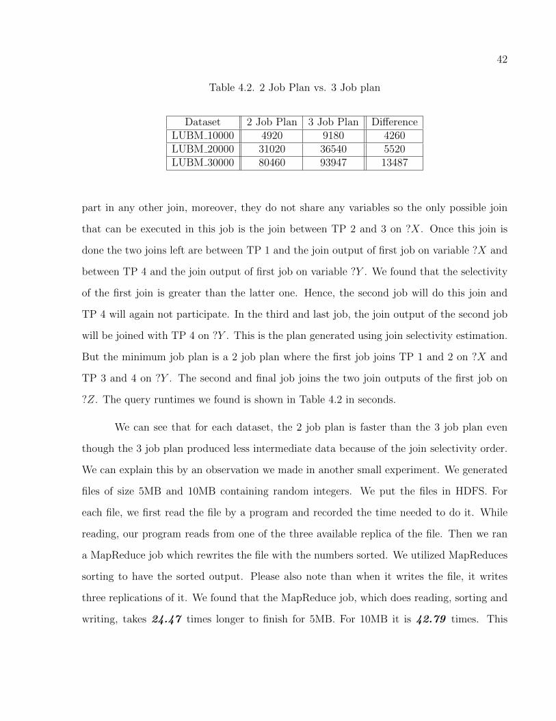
42
Table 4.2. 2 Job Plan vs. 3 Job plan
Dataset 2 Job Plan 3 Job Plan DifferenceLUBM 10000 4920 9180 4260LUBM 20000 31020 36540 5520LUBM 30000 80460 93947 13487
part in any other join, moreover, they do not share any variables so the only possible join
that can be executed in this job is the join between TP 2 and 3 on ?X. Once this join is
done the two joins left are between TP 1 and the join output of first job on variable ?X and
between TP 4 and the join output of first job on variable ?Y . We found that the selectivity
of the first join is greater than the latter one. Hence, the second job will do this join and
TP 4 will again not participate. In the third and last job, the join output of the second job
will be joined with TP 4 on ?Y . This is the plan generated using join selectivity estimation.
But the minimum job plan is a 2 job plan where the first job joins TP 1 and 2 on ?X and
TP 3 and 4 on ?Y . The second and final job joins the two join outputs of the first job on
?Z. The query runtimes we found is shown in Table 4.2 in seconds.
We can see that for each dataset, the 2 job plan is faster than the 3 job plan even
though the 3 job plan produced less intermediate data because of the join selectivity order.
We can explain this by an observation we made in another small experiment. We generated
files of size 5MB and 10MB containing random integers. We put the files in HDFS. For
each file, we first read the file by a program and recorded the time needed to do it. While
reading, our program reads from one of the three available replica of the file. Then we ran
a MapReduce job which rewrites the file with the numbers sorted. We utilized MapReduces
sorting to have the sorted output. Please also note than when it writes the file, it writes
three replications of it. We found that the MapReduce job, which does reading, sorting and
writing, takes 24.47 times longer to finish for 5MB. For 10MB it is 42.79 times. This
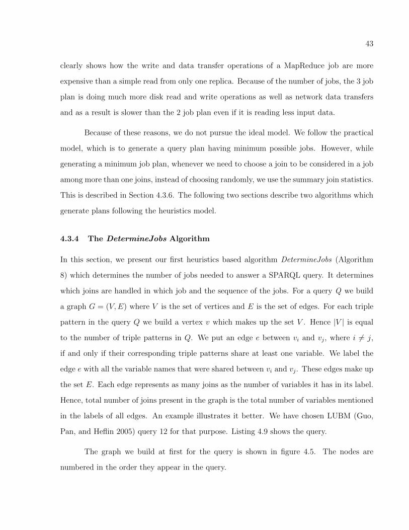
43
clearly shows how the write and data transfer operations of a MapReduce job are more
expensive than a simple read from only one replica. Because of the number of jobs, the 3 job
plan is doing much more disk read and write operations as well as network data transfers
and as a result is slower than the 2 job plan even if it is reading less input data.
Because of these reasons, we do not pursue the ideal model. We follow the practical
model, which is to generate a query plan having minimum possible jobs. However, while
generating a minimum job plan, whenever we need to choose a join to be considered in a job
among more than one joins, instead of choosing randomly, we use the summary join statistics.
This is described in Section 4.3.6. The following two sections describe two algorithms which
generate plans following the heuristics model.
4.3.4 The DetermineJobs Algorithm
In this section, we present our first heuristics based algorithm DetermineJobs (Algorithm
8) which determines the number of jobs needed to answer a SPARQL query. It determines
which joins are handled in which job and the sequence of the jobs. For a query Q we build
a graph G = (V,E) where V is the set of vertices and E is the set of edges. For each triple
pattern in the query Q we build a vertex v which makes up the set V . Hence |V | is equal
to the number of triple patterns in Q. We put an edge e between vi and vj, where i 6= j,
if and only if their corresponding triple patterns share at least one variable. We label the
edge e with all the variable names that were shared between vi and vj. These edges make up
the set E. Each edge represents as many joins as the number of variables it has in its label.
Hence, total number of joins present in the graph is the total number of variables mentioned
in the labels of all edges. An example illustrates it better. We have chosen LUBM (Guo,
Pan, and Heflin 2005) query 12 for that purpose. Listing 4.9 shows the query.
The graph we build at first for the query is shown in figure 4.5. The nodes are
numbered in the order they appear in the query.
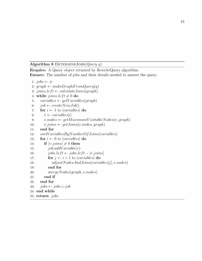
44
Algorithm 8 DetermineJobs(Query q)
Require: A Query object returned by RewriteQuery algorithm.Ensure: The number of jobs and their details needed to answer the query.
1: jobs← φ2: graph← makeGraphFromQuery(q)3: joins left← calculateJoins(graph)4: while joins left 6= 0 do5: variables← getV ariables(graph)6: job← createNewJob()7: for i← 1 to |variables| do8: v ← variables[i]9: v.nodes← getMaximumV isitableNodes(v, graph)10: v.joins← getJoins(v.nodes, graph)11: end for12: sortV ariablesByNumberOfJoins(variables)13: for i← 0 to |variables| do14: if |v.joins| 6= 0 then15: job.addV ariable(v)16: jobs left← jobs left− |v.joins]17: for j ← i+ 1 to |variables| do18: adjustNodesAndJoins(variables[j], v.nodes)19: end for20: mergeNodes(graph, v.nodes)21: end if22: end for23: jobs← jobs ∪ job24: end while25: return jobs
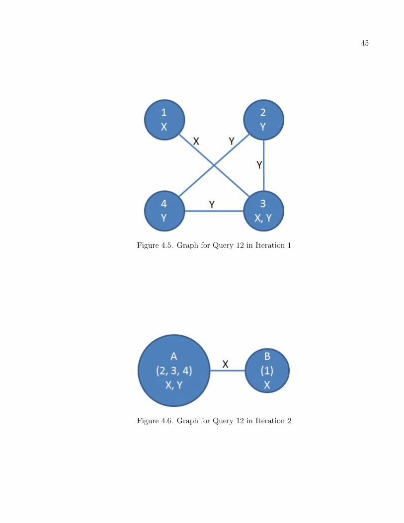
45
Figure 4.5. Graph for Query 12 in Iteration 1
Figure 4.6. Graph for Query 12 in Iteration 2
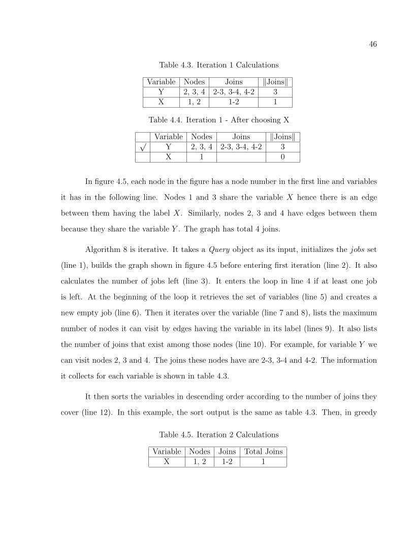
46
Table 4.3. Iteration 1 Calculations
Variable Nodes Joins ‖Joins‖Y 2, 3, 4 2-3, 3-4, 4-2 3X 1, 2 1-2 1
Table 4.4. Iteration 1 - After choosing X
Variable Nodes Joins ‖Joins‖√Y 2, 3, 4 2-3, 3-4, 4-2 3X 1 0
In figure 4.5, each node in the figure has a node number in the first line and variables
it has in the following line. Nodes 1 and 3 share the variable X hence there is an edge
between them having the label X. Similarly, nodes 2, 3 and 4 have edges between them
because they share the variable Y . The graph has total 4 joins.
Algorithm 8 is iterative. It takes a Query object as its input, initializes the jobs set
(line 1), builds the graph shown in figure 4.5 before entering first iteration (line 2). It also
calculates the number of jobs left (line 3). It enters the loop in line 4 if at least one job
is left. At the beginning of the loop it retrieves the set of variables (line 5) and creates a
new empty job (line 6). Then it iterates over the variable (line 7 and 8), lists the maximum
number of nodes it can visit by edges having the variable in its label (lines 9). It also lists
the number of joins that exist among those nodes (line 10). For example, for variable Y we
can visit nodes 2, 3 and 4. The joins these nodes have are 2-3, 3-4 and 4-2. The information
it collects for each variable is shown in table 4.3.
It then sorts the variables in descending order according to the number of joins they
cover (line 12). In this example, the sort output is the same as table 4.3. Then, in greedy
Table 4.5. Iteration 2 Calculations
Variable Nodes Joins Total JoinsX 1, 2 1-2 1
47
fashion, it iterates over the variables and chooses a variables if the variable covers at least
one join (line 13 and 14). In each iteration, after it chooses a variable, it eliminates all
the nodes it covers from subsequent variable entries (lines 17 to 19). It then calculates the
number of joins still left in the graph (line 16). For example, once the algorithm chooses the
variable Y , the nodes and joins for X becomes like table 4.4.
It also merges the nodes visited by the chosen variable in the graph (line 20). Hence,
after choosing Y it will not choose X as it does not cover any join any more. Here the inner
loop terminates. The joins it picked are the joins that will be done in a job. The algorithm
then checks whether any join is not picked (line 4). If such is the case, then more jobs are
needed and so the algorithm goes to the next iteration.
At the beginning of the subsequent iteration it again builds a graph from the graph
of the previous iteration but this time the nodes which took part in joins by one variable
will be collapsed into a single node. For our example, nodes 2, 3 and 4 took part in joins by
Y . So they will collapse and form a single node. For clarity, we name this collapsed node
as A and the remaining node 1 of the graph in figure 4.5 as B. The new graph we get like
this is shown in figure 4.6. The graph has total 1 join. We have listed the nodes which were
collapsed in braces.
After building the graph, the algorithm moves on to list the maximum number of
nodes, joins and total number of joins each variable covers. This is shown in table 4.5. The
algorithm chooses X and that covers all the joins of the graph. The algorithm determines
that no more job is needed and returns the job collection.
4.3.5 The Relaxed-Bestplan Algorithm
In this section, first we define the query plan generation problem, and show that generating
the best (i.e., least cost) query plan for the ideal model (section 4.3.1) as well as for the
48
practical model (section 4.3.3) is computationally expensive. Then, we will present a heuristic
and a greedy approach to generate an approximate solution to generate the best plan.
Running example: We will use the following query as a running example in this
section.
Listing 4.12. Running Example
SELECT ?V, ?X, ?Y, ? Z WHERE{?X rd f : type ub : GraduateStudent?Y rd f : type ub : Un ive r s i ty?Z ?V ub : Department?X ub : memberOf ?Z?X ub : undergraduateDegreeFrom ?Y}
In order to simplify the notations, we will only refer to the TPs by the variable in that
pattern. For example, the first TP (?X rdf:type ub:GraduateStudent) will be represented as
simply X. Also, in the simplified version, the whole query would be represented as follows:
{X,Y,Z,XZ,XY}. We shall use the notation join(XY,X) to denote a join operation between
the two TPs XY and X on the common variable X.
Definition 7 (The minimum cost plan generation problem). (Bestplan problem) For a given
query, the Bestplan problem is to generate a job plan so that the total cost of the jobs is
minimized. Note that Bestplan considers the more general case where each job has some cost
associated with it (i.e., the ideal model).
Example: Given the query in our running example, two possible job plans are as
follows:
Plan 1: job1 = join(X,XZ,XY), resultant TPs = {Y,Z,YZ}. job2 = join(Y,YZ),
resultant TPs = {Z,Z}. job3 = join(Z,Z). Total cost = cost(job1)+cost(job2)+cost(job3).
Plan 2: job1 = join(XZ,Z) and join(XY,Y) resultant TPs = {X,X,X}. job2 =
join(X,X,X). Total cost = cost(job1)+cost(job2).
49
The Bestplan problem is to find the least cost job plan among all possible job plans.
Related terms:
Definition 8 (Joining variable). A variable that is common in two or more triple patterns.
For example, in the running example query, X,Y,Z are joining variables, but V is not.
Definition 9 (Complete elimination). A join operation that eliminates a joining variable.
For example, in the example query, Y can be completely eliminated if we join (XY,Y).
Definition 10 (Partial elimination). A join operation that partially eliminates a joining vari-
able. For example, in the example query, if we perform join(XY,Y) and join(X,ZX) in the
same job, the resultant triple patterns would be {X,Z,X}. Therefore, Y will be completely
eliminated, but X will be partially eliminated. So, the join(X,ZX) performs a partial elimi-
nation.
Definition 11 (E-count(v)). E-count(v) is the number of joining variables in the resul-
tant triple pattern after a complete elimination of variable v. In the running example,
join(X,XY,XZ) completely eliminates X, and the resultant triple pattern (YZ) has two join-
ing variables Y and Z. So, E-count(X) = 2. Similarly, E-count(Y)=1 and E-count(Z) =
1.
4.3.5.1 Computational complexity of Bestplan
It can be shown that generating the least cost query plan is computationally expensive, since
the search space is exponentially large. At first, we formulate the problem, and then show
its complexity.
Problem formulation: We formulate Bestplan as a search problem. Let G = (V,E)
be a weighted directed graph, where each vertex vi ∈ V represents a state of the triple
patterns, and each edge ei = (vi1 , vi2) ∈ E represents a job that makes a transition from
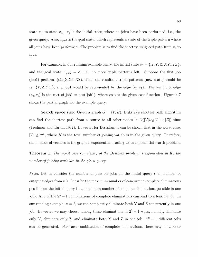
50
state vi1 to state vi2 . v0 is the initial state, where no joins have been performed, i.e., the
given query. Also, vgoal is the goal state, which represents a state of the triple pattern where
all joins have been performed. The problem is to find the shortest weighted path from v0 to
vgoal.
For example, in our running example query, the initial state v0 = {X, Y, Z,XY,XZ},
and the goal state, vgoal = φ, i.e., no more triple patterns left. Suppose the first job
(job1) performs join(X,XY,XZ). Then the resultant triple patterns (new state) would be
v1={Y, Z, Y Z}, and job1 would be represented by the edge (v0, v1). The weight of edge
(v0, v1) is the cost of job1 = cost(job1), where cost is the given cost function. Figure 4.7
shows the partial graph for the example query.
Search space size: Given a graph G = (V,E), Dijkstra’s shortest path algorithm
can find the shortest path from a source to all other nodes in O(|V |log|V | + |E|) time
(Fredman and Tarjan 1987). However, for Bestplan, it can be shown that in the worst case,
|V | ≥ 2K , where K is the total number of joining variables in the given query. Therefore,
the number of vertices in the graph is exponential, leading to an exponential search problem.
Theorem 1. The worst case complexity of the Bestplan problem is exponential in K, the
number of joining variables in the given query.
Proof. Let us consider the number of possible jobs on the initial query (i.e., number of
outgoing edges from v0). Let n be the maximum number of concurrent complete eliminations
possible on the initial query (i.e., maximum number of complete eliminations possible in one
job). Any of the 2n − 1 combinations of complete eliminations can lead to a feasible job. In
our running example, n = 2, we can completely eliminate both Y and Z concurrently in one
job. However, we may choose among these eliminations in 22 − 1 ways, namely, eliminate
only Y, eliminate only Z, and eliminate both Y and Z in one job. 22 − 1 different jobs
can be generated. For each combination of complete eliminations, there may be zero or
51
Figure 4.7. The (partial) graph for the running example query with the initial state and allstates adjacent to it.
52
more possible partial eliminations. Again, we may choose any combination of those partial
eliminations. For example, if we choose to eliminate Y only, then we can partially eliminate
X. We may or may not choose to partially eliminate X, leading to two different job patterns.
Therefore, the minimum number of possible jobs (outgoing edges) on the initial query (i.e.,
v0) is 2n−1. Note that each of these jobs (i.e., edges) will lead to a unique state (i.e., vertex).
Therefore, the number of vertices adjacent to v0 is at least 2n − 1. In the worst case, n=K,
meaning, the minimum number of vertices adjacent to v0 is 2K − 1. Note that we are not
even counting the vertices (i.e., states) that are generated from these 2K − 1 vertices. The
complexity of computing the least cost path from v0 to vgoal is at least O(|E|) because every
edge must be considered at least once lest the algorithm miss a least-cost path that contains
that edge. Since in the worst case the minimum number of vertices adjacent to v0 is 2K − 1,
|E| is at least O(2K), which is exponential. Hence, every solution to the Bestplan problem
is at least exponential in the number of joining variables in the worst case.
However, we may still solve Bestplan in reasonable amount of time if K is small. This
solution would involve generating the graph G and then finding the shortest path from v0 to
vgoal.
4.3.5.2 Relaxed Bestplan problem and approximate solution
In the Relaxed Bestplan problem, we assume uniform cost for all jobs. Although this relax-
ation does not reduce the search space, the problem is reduced to finding a job plan having
the minimum number of jobs. Note that this is the problem for the practical version of the
model (Section 4.3.3).
Definition 12 (Relaxed Bestplan problem). The Relaxed Bestplan problem is to find the job
plan that has the minimum number of jobs.
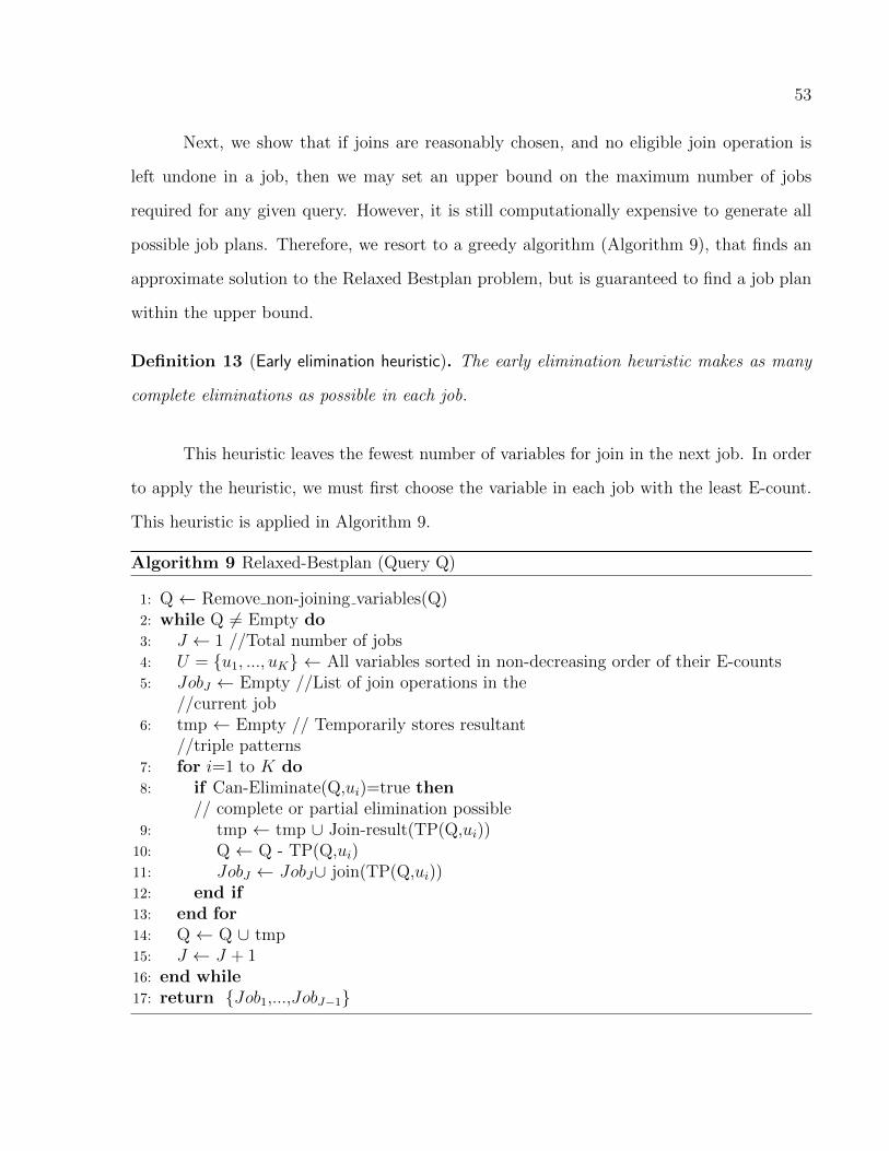
53
Next, we show that if joins are reasonably chosen, and no eligible join operation is
left undone in a job, then we may set an upper bound on the maximum number of jobs
required for any given query. However, it is still computationally expensive to generate all
possible job plans. Therefore, we resort to a greedy algorithm (Algorithm 9), that finds an
approximate solution to the Relaxed Bestplan problem, but is guaranteed to find a job plan
within the upper bound.
Definition 13 (Early elimination heuristic). The early elimination heuristic makes as many
complete eliminations as possible in each job.
This heuristic leaves the fewest number of variables for join in the next job. In order
to apply the heuristic, we must first choose the variable in each job with the least E-count.
This heuristic is applied in Algorithm 9.
Algorithm 9 Relaxed-Bestplan (Query Q)
1: Q ← Remove non-joining variables(Q)2: while Q 6= Empty do3: J ← 1 //Total number of jobs4: U = {u1, ..., uK} ← All variables sorted in non-decreasing order of their E-counts5: JobJ ← Empty //List of join operations in the
//current job6: tmp ← Empty // Temporarily stores resultant
//triple patterns7: for i=1 to K do8: if Can-Eliminate(Q,ui)=true then
// complete or partial elimination possible9: tmp ← tmp ∪ Join-result(TP(Q,ui))10: Q ← Q - TP(Q,ui)11: JobJ ← JobJ∪ join(TP(Q,ui))12: end if13: end for14: Q ← Q ∪ tmp15: J ← J + 116: end while17: return {Job1,...,JobJ−1}
54
Description of Algorithm 9:. The algorithm starts by removing all the non-joining
variables from the query Q. In our running example, Q={X,Y,VZ,XY,XZ}, and removing
the non-joining variable V makes Q={X,Y,Z,XY,XZ}. In the while loop, the job plan is
generated, starting from Job1. In line 4, we sort the variables according to their E-count. The
sorted variables are: U = {Y, Z,X}, since Y, and Z have E-count = 1, and X has E-count=2.
For each job, the list of join operations are stored in the variable JobJ , where J is the ID of
the current job. Also, a temporary variable tmp is used to store the resultant triples of the
joins to be performed in the current job (line 6). In the for loop, each variable is checked to
see if the variable can be completely or partially eliminated (line 8). If yes, we store the join
result in the temporary variable (line 9), update Q (line 10) and add this join to the current
job (line 11). In our running example, this results in the following operations. Iteration 1 of
the for loop: u1 (= Y) can be completely eliminated. Here TP(Q,Y) = the triple patterns
in Q containing Y = {Y,XY}. Join-result(TP(Q,Y)) = Join-result({Y,XY}) = resultant
triple after the join(Y,XY) = X. So, tmp = {X}. Q = Q - TP(Q,Y) = {X,Y,Z,XY,XZ} -
{Y,XY} = {X,Z,XZ}. Job1 = {join(Y,XY)}. Iteration 2 of the for loop: u2 (= Z) can be
completely eliminated. Here TP(Q,Z) = {Z,XZ}, and Join-result({Z,XZ}) = X. So, tmp =
{X,X}, Q = Q - TP(Q,Z) = {X,Z,XZ} - {Z,ZX} = {X}, Job1 = {join(Y,XY),join(Z,XZ)}.
Iteration 3 of the for loop: u3 (= X) cannot be completely or partially eliminated, since there
is no other TP left to join with it. Therefore, when the for loop terminates, we have Job1
= {join(Y,XY),join(Z,XZ)}, and Q = {X,X,X}. In the second iteration of the while loop,
we will have Job2 = join(X,X,X). Since after this join, Q becomes Empty, the while loop is
exited. Finally, {Job1, Job2} are returned from the algorithm.
Theorem 2. For any given query Q, containing K joining variables and N triple patterns,
Algorithm Relaxed-Bestplan(Q) generates a job plan containing at most J jobs, where
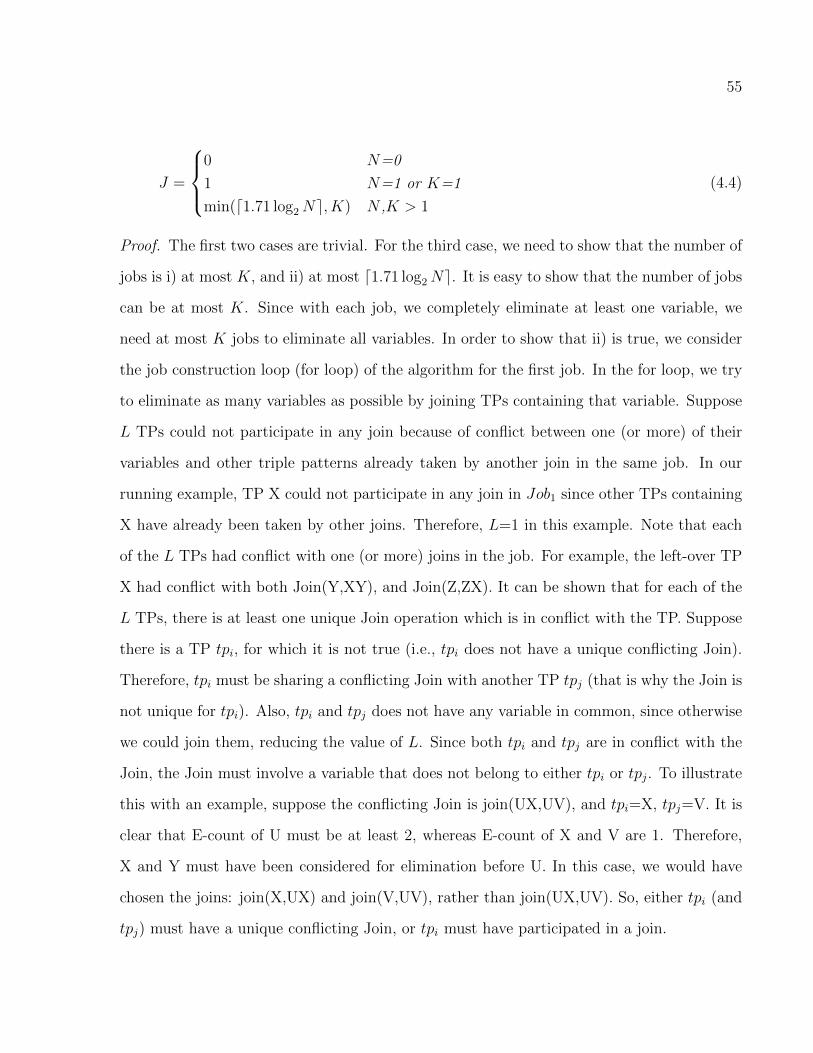
55
J =
0 N=0
1 N=1 or K=1
min(d1.71 log2Ne, K) N ,K > 1
(4.4)
Proof. The first two cases are trivial. For the third case, we need to show that the number of
jobs is i) at most K, and ii) at most d1.71 log2Ne. It is easy to show that the number of jobs
can be at most K. Since with each job, we completely eliminate at least one variable, we
need at most K jobs to eliminate all variables. In order to show that ii) is true, we consider
the job construction loop (for loop) of the algorithm for the first job. In the for loop, we try
to eliminate as many variables as possible by joining TPs containing that variable. Suppose
L TPs could not participate in any join because of conflict between one (or more) of their
variables and other triple patterns already taken by another join in the same job. In our
running example, TP X could not participate in any join in Job1 since other TPs containing
X have already been taken by other joins. Therefore, L=1 in this example. Note that each
of the L TPs had conflict with one (or more) joins in the job. For example, the left-over TP
X had conflict with both Join(Y,XY), and Join(Z,ZX). It can be shown that for each of the
L TPs, there is at least one unique Join operation which is in conflict with the TP. Suppose
there is a TP tpi, for which it is not true (i.e., tpi does not have a unique conflicting Join).
Therefore, tpi must be sharing a conflicting Join with another TP tpj (that is why the Join is
not unique for tpi). Also, tpi and tpj does not have any variable in common, since otherwise
we could join them, reducing the value of L. Since both tpi and tpj are in conflict with the
Join, the Join must involve a variable that does not belong to either tpi or tpj. To illustrate
this with an example, suppose the conflicting Join is join(UX,UV), and tpi=X, tpj=V. It is
clear that E-count of U must be at least 2, whereas E-count of X and V are 1. Therefore,
X and Y must have been considered for elimination before U. In this case, we would have
chosen the joins: join(X,UX) and join(V,UV), rather than join(UX,UV). So, either tpi (and
tpj) must have a unique conflicting Join, or tpi must have participated in a join.

56
To summarize the fact, there have been at least M >= L joins selected in Job1.
So, the total number of TPs left after executing all the joins of Job1 is M+L. Note that
each of the M joins involves at least 2 TPs. Therefore, 2M + L ≤ N , where N is the total
number of TPs in the given query. From the above discussion, we come-up with the following
relationships:
2M + L ≤ N ⇒ 2(L+ ε) + L ≤ N (Letting ε ≥ 0)
⇒ 3L+ 2ε ≤ N
⇒ 2L+4
3ε ≤ 2
3N (Multiplying both sides with 2/3)
⇒ 2L+ ε ≤ 2
3N ⇒M + L ≤ 2
3N
So, the first job, as well as each remaining jobs reduce the number of TPs to at least
two-third. Therefore, there is a integer J such that:
(2
3)JN ≥ 1 ≥ (
2
3)J+1N ⇒ (
3
2)J ≤ N ≤ (
3
2)J+1
⇒ J ≤ log3/2N = 1.71 log2N ≤ J + 1
So, the total number of jobs, J is also bounded by d1.71 log2Ne.
In most real world scenarios, we can safely assume that more than 100 triples in
a query is extremely rare. So, the maximum number of jobs required with the Relaxed-
Bestplan algorithm is at most 12.
Worst case ratio between number of jobs returned by Relaxed-Bestplan
algorithm and the actual least number of jobs: While in all our experiments the
57
Relaxed-Bestplan algorithm returned the plans with the least number of jobs possible, there
might be cases where the plan might not be the optimal one in terms of the number of jobs.
We are working on to determine the worst case ratio between number of jobs returned by
Relaxed-Bestplan algorithm and the actual least number of jobs. As of now, the problem to
determine this ratio is open.
Complexity of the Relaxed-Bestplan algorithm: The outer loop (while loop)
runs at most J times, where J is the upper bound of the number of jobs. The inner (for)
loop runs at most K times, where K is the number of joining variables in the given query.
The sorting requires O(K logK) time. Therefore, the overall complexity of the algorithm is
O(K(J + logK)).
4.3.6 Breaking Ties by Summary Statistics
We frequently face situations where we need to choose a join for multiple join options. These
choices can occur when both query plans (i.e. join orderings) require the minimum number
of jobs. For example, the query shown in Listing 4.13 poses such a situation.
Listing 4.13. Query Having Tie Situation
?X rd f : type ub : F u l l P r o f e s s o r .?X ub : advisorOf ?Y .?Y rd f : type ub : ResearchAss i s tant .
The second triple pattern in the query makes it impossible to answer solve the query
with only one job. There are only two possible plans: we can join the first two triple patterns
on X first and then join its output with the last triple pattern on Y or we can join the last
two patterns first on Y and then join its output with the first pattern on X. In such a
situation, instead of randomly choosing a join variable for the first job, we use join summary
statistics for a pair of predicates. We select the join for the first job which is more selective
to break the tie. The join summary statistics we use is described in (Stocker, Seaborne,
Bernstein, Kiefer, and Reynolds 2008).
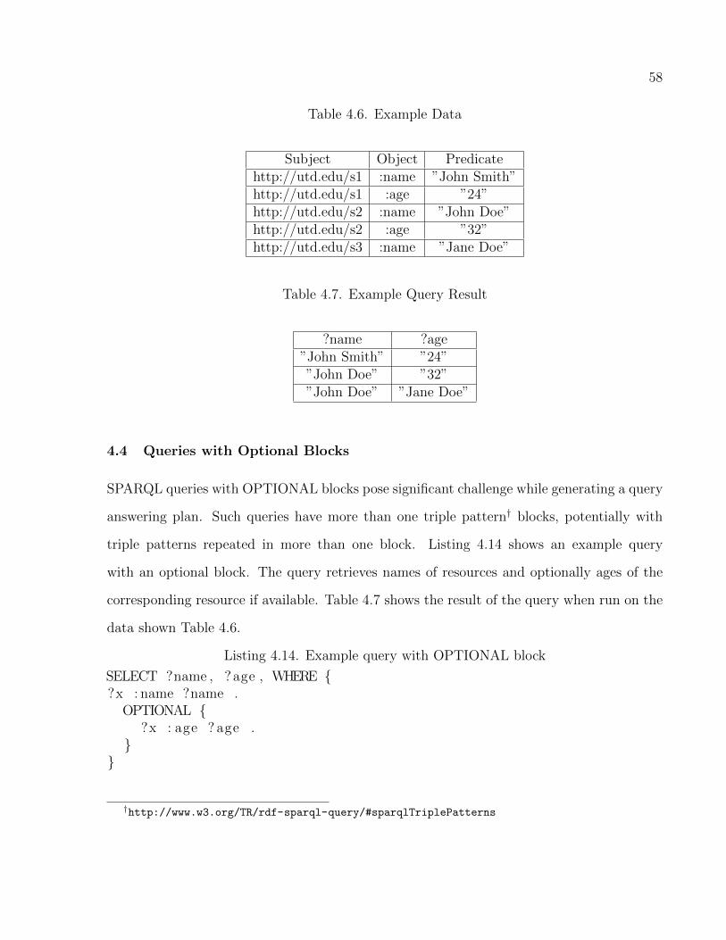
58
Table 4.6. Example Data
Subject Object Predicatehttp://utd.edu/s1 :name ”John Smith”http://utd.edu/s1 :age ”24”http://utd.edu/s2 :name ”John Doe”http://utd.edu/s2 :age ”32”http://utd.edu/s3 :name ”Jane Doe”
Table 4.7. Example Query Result
?name ?age”John Smith” ”24””John Doe” ”32””John Doe” ”Jane Doe”
4.4 Queries with Optional Blocks
SPARQL queries with OPTIONAL blocks pose significant challenge while generating a query
answering plan. Such queries have more than one triple pattern† blocks, potentially with
triple patterns repeated in more than one block. Listing 4.14 shows an example query
with an optional block. The query retrieves names of resources and optionally ages of the
corresponding resource if available. Table 4.7 shows the result of the query when run on the
data shown Table 4.6.
Listing 4.14. Example query with OPTIONAL block
SELECT ?name , ?age , WHERE {?x : name ?name .
OPTIONAL {?x : age ? age .
}}
†http://www.w3.org/TR/rdf-sparql-query/#sparqlTriplePatterns
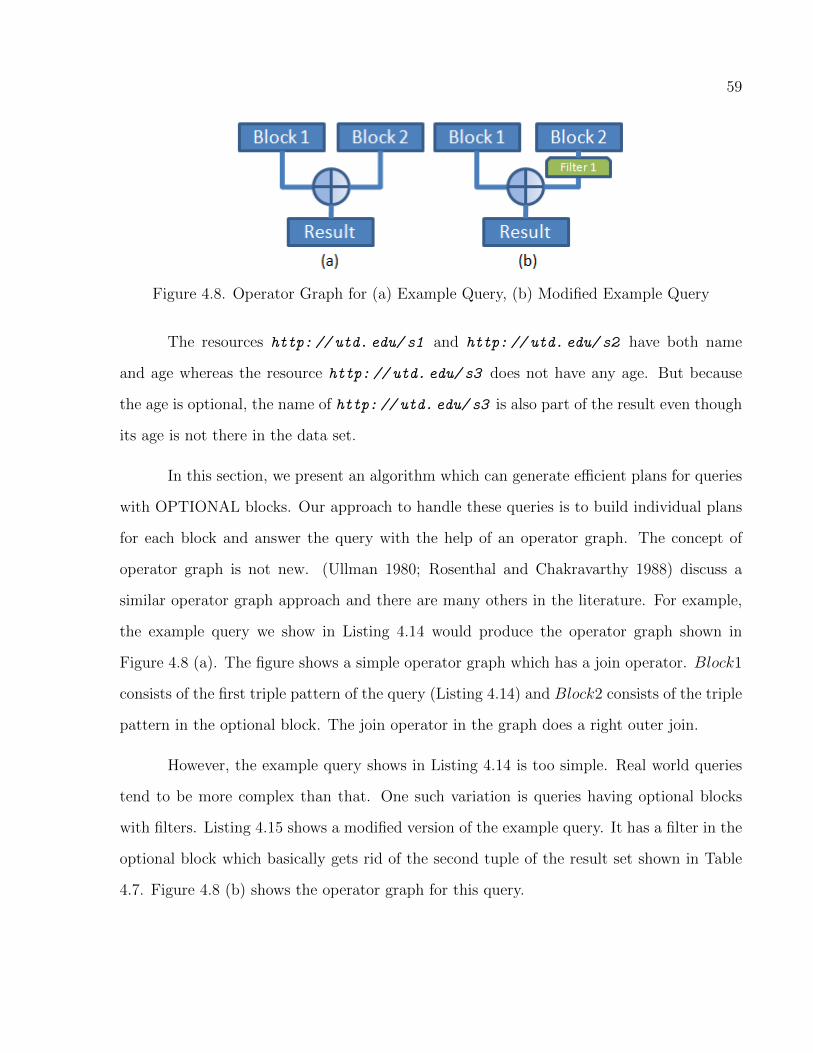
59
Figure 4.8. Operator Graph for (a) Example Query, (b) Modified Example Query
The resources http: // utd. edu/ s1 and http: // utd. edu/ s2 have both name
and age whereas the resource http: // utd. edu/ s3 does not have any age. But because
the age is optional, the name of http: // utd. edu/ s3 is also part of the result even though
its age is not there in the data set.
In this section, we present an algorithm which can generate efficient plans for queries
with OPTIONAL blocks. Our approach to handle these queries is to build individual plans
for each block and answer the query with the help of an operator graph. The concept of
operator graph is not new. (Ullman 1980; Rosenthal and Chakravarthy 1988) discuss a
similar operator graph approach and there are many others in the literature. For example,
the example query we show in Listing 4.14 would produce the operator graph shown in
Figure 4.8 (a). The figure shows a simple operator graph which has a join operator. Block1
consists of the first triple pattern of the query (Listing 4.14) and Block2 consists of the triple
pattern in the optional block. The join operator in the graph does a right outer join.
However, the example query shows in Listing 4.14 is too simple. Real world queries
tend to be more complex than that. One such variation is queries having optional blocks
with filters. Listing 4.15 shows a modified version of the example query. It has a filter in the
optional block which basically gets rid of the second tuple of the result set shown in Table
4.7. Figure 4.8 (b) shows the operator graph for this query.
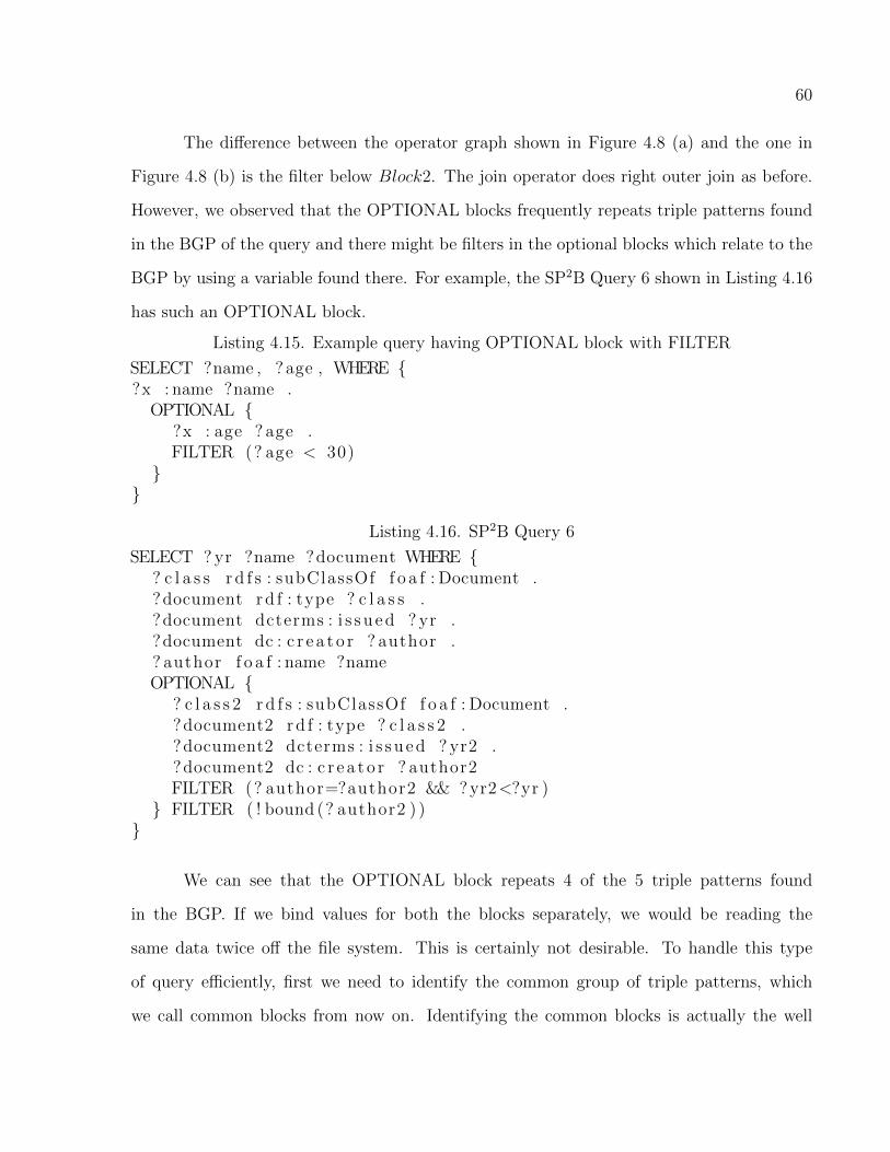
60
The difference between the operator graph shown in Figure 4.8 (a) and the one in
Figure 4.8 (b) is the filter below Block2. The join operator does right outer join as before.
However, we observed that the OPTIONAL blocks frequently repeats triple patterns found
in the BGP of the query and there might be filters in the optional blocks which relate to the
BGP by using a variable found there. For example, the SP2B Query 6 shown in Listing 4.16
has such an OPTIONAL block.
Listing 4.15. Example query having OPTIONAL block with FILTER
SELECT ?name , ?age , WHERE {?x : name ?name .
OPTIONAL {?x : age ? age .FILTER (? age < 30)
}}
Listing 4.16. SP2B Query 6
SELECT ? yr ?name ?document WHERE {? c l a s s r d f s : subClassOf f o a f : Document .?document rd f : type ? c l a s s .?document dcterms : i s s u e d ? yr .?document dc : c r e a t o r ? author .? author f o a f : name ?nameOPTIONAL {
? c l a s s 2 r d f s : subClassOf f o a f : Document .?document2 rd f : type ? c l a s s 2 .?document2 dcterms : i s s u ed ? yr2 .?document2 dc : c r e a t o r ? author2FILTER (? author=?author2 && ? yr2<?yr )
} FILTER ( ! bound (? author2 ) )}
We can see that the OPTIONAL block repeats 4 of the 5 triple patterns found
in the BGP. If we bind values for both the blocks separately, we would be reading the
same data twice off the file system. This is certainly not desirable. To handle this type
of query efficiently, first we need to identify the common group of triple patterns, which
we call common blocks from now on. Identifying the common blocks is actually the well
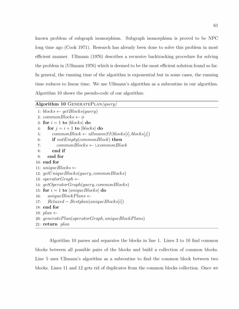
61
known problem of subgraph isomorphism. Subgraph isomorphism is proved to be NPC
long time ago (Cook 1971). Research has already been done to solve this problem in most
efficient manner. Ullmann (1976) describes a recursive backtracking procedure for solving
the problem in (Ullmann 1976) which is deemed to be the most efficient solution found so far.
In general, the running time of the algorithm is exponential but in some cases, the running
time reduces to linear time. We use Ullmann’s algorithm as a subroutine in our algorithm.
Algorithm 10 shows the pseudo-code of our algorithm:
Algorithm 10 GeneratePlan(query)
1: blocks← getBlocks(query)2: commonBlocks← φ3: for i = 1 to |blocks| do4: for j = i+ 1 to |blocks| do5: commonBlock ← ullmannSI(blocks[i], blocks[j])6: if notEmpty(commonBlock) then7: commonBlocks← ∪commonBlock8: end if9: end for10: end for11: uniqueBlocks←12: getUniqueBlocks(query, commonBlocks)13: operatorGraph←14: getOperatorGraph(query, commonBlocks)15: for i = 1 to |uniqueBlocks| do16: uniqueBlockP lans←17: Relaxed−Bestplan(uniqueBlocks[i])18: end for19: plan←20: generateP lan(operatorGraph, uniqueBlockP lans)21: return plan
Algorithm 10 parses and separates the blocks in line 1. Lines 3 to 10 find common
blocks between all possible pairs of the blocks and build a collection of common blocks.
Line 5 uses Ullmann’s algorithm as a subroutine to find the common block between two
blocks. Lines 11 and 12 gets rid of duplicates from the common blocks collection. Once we
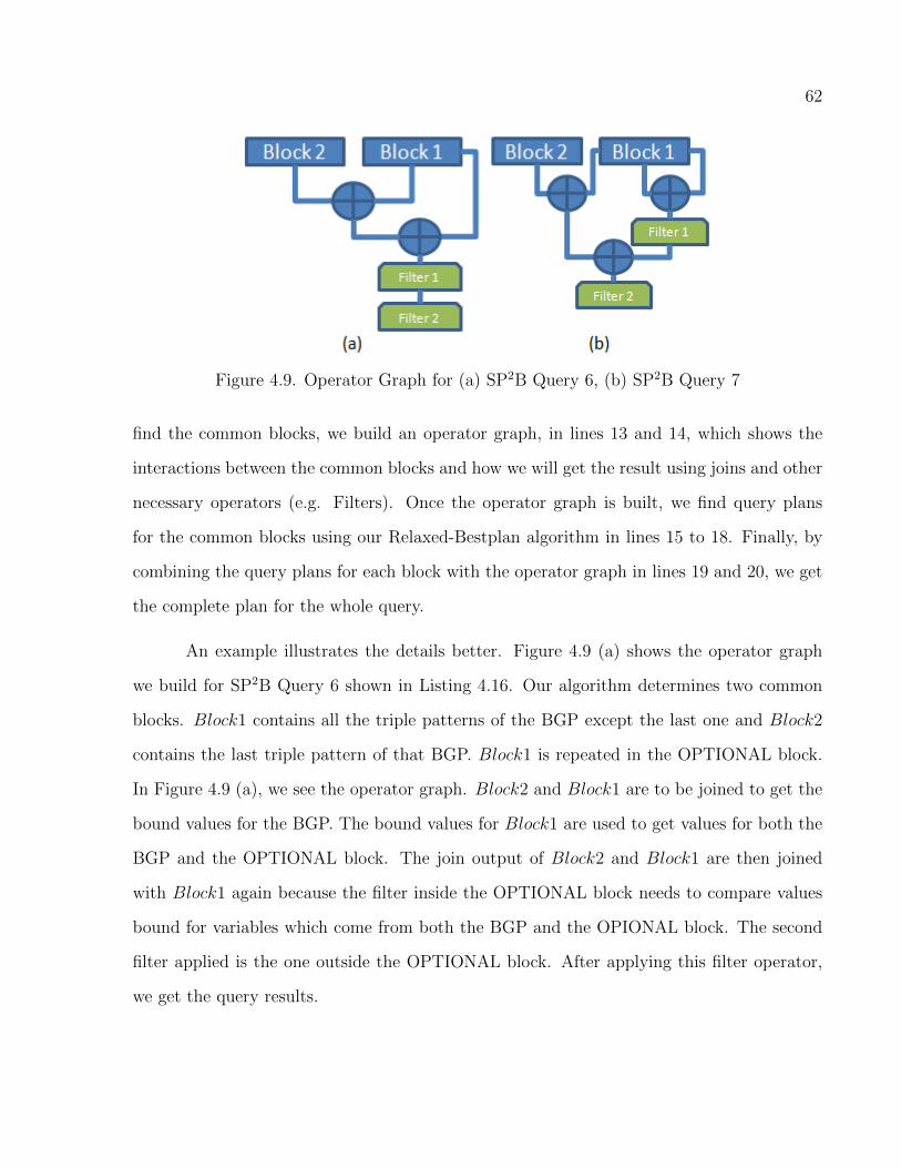
62
Figure 4.9. Operator Graph for (a) SP2B Query 6, (b) SP2B Query 7
find the common blocks, we build an operator graph, in lines 13 and 14, which shows the
interactions between the common blocks and how we will get the result using joins and other
necessary operators (e.g. Filters). Once the operator graph is built, we find query plans
for the common blocks using our Relaxed-Bestplan algorithm in lines 15 to 18. Finally, by
combining the query plans for each block with the operator graph in lines 19 and 20, we get
the complete plan for the whole query.
An example illustrates the details better. Figure 4.9 (a) shows the operator graph
we build for SP2B Query 6 shown in Listing 4.16. Our algorithm determines two common
blocks. Block1 contains all the triple patterns of the BGP except the last one and Block2
contains the last triple pattern of that BGP. Block1 is repeated in the OPTIONAL block.
In Figure 4.9 (a), we see the operator graph. Block2 and Block1 are to be joined to get the
bound values for the BGP. The bound values for Block1 are used to get values for both the
BGP and the OPTIONAL block. The join output of Block2 and Block1 are then joined
with Block1 again because the filter inside the OPTIONAL block needs to compare values
bound for variables which come from both the BGP and the OPIONAL block. The second
filter applied is the one outside the OPTIONAL block. After applying this filter operator,
we get the query results.
63
We can handle any query with OPTIONAL blocks this way. A query might have
nested OPTIONAL blocks and our approach can handle those queries too. We use Hadoop
jobs to do the joins and apply the operators (e.g. Filter) in the query operator graph.
However, the number of Hadoop jobs needed to do these operation is not necessarily equal
to the number of operators. For the example operator graph shown in Figure 4.9 (a), we
would need two jobs to do the joins and the filters. We can apply the filters in the same job
which does the 2nd join. In general only join operators need separate Hadoop jobs. Other
operators can be applied in the job doing the join which produces the output to be worked
on by the operators.
An optional block might have multiple nested optional blocks inside it. Our approach
can handle any number of such nesting in the optional blocks. Listing 4.17 shows SP2B Query
7 which has a nested optional block inside the first optional block. Our algorithm identifies
two unique blocks from the query. Block1 contains the third triple pattern of the BGP
?doc dc : title ?title. Block2 contains the rest four triple patterns of the BGP. Block2 is
repeated twice in the optional blocks. The operator graph we build for this query is shown
in Figure 4.9 (b). We can see that Block2 is input three times, hence we can avoid reading
from the disk thrice. Instead we only read data from the disk once for the block and reuse
it three times. This significantly improves query running time.
Listing 4.17. SP2B Query 7
SELECT DISTINCT ? t i t l eWHERE {
? c l a s s r d f s : subClassOf f o a f : Document .?doc rd f : type ? c l a s s .?doc dc : t i t l e ? t i t l e .?bag2 ?member2 ?doc .? doc2 dcterms : r e f e r e n c e s ?bag2OPTIONAL {
? c l a s s 3 r d f s : subClassOf f o a f : Document .? doc3 rd f : type ? c l a s s 3 .? doc3 dcterms : r e f e r e n c e s ?bag3 .?bag3 ?member3 ?doc
64
OPTIONAL {? c l a s s 4 r d f s : subClassOf f o a f : Document .? doc4 rd f : type ? c l a s s 4 .? doc4 dcterms : r e f e r e n c e s ?bag4 .?bag4 ?member4 ? doc3
} FILTER ( ! bound (? doc4 ) )} FILTER ( ! bound (? doc3 ) )
}
Due to space constraint, we do not show the details of the trivial algorithm which
builds the operator graph. Such algorithms are commonly found in the relational database
literature.
4.5 MapReduce Join Execution
In this section, we discuss how we implement the joins needed to answer SPARQL queries
using MapReduce framework of Hadoop. Algorithm 9 determines the number of jobs re-
quired to answer a query. It returns an ordered set of jobs. Each job has associated input
information. The Job Handler component of our MapReduce framework runs the jobs in the
sequence they appear in the ordered set. The output file of one job is the input of the next.
The output file of the last job has the answer to the query.
Listing 4.18. LUBM Query 2
SELECT ?X, ?Y, ?Z WHERE {?X rd f : type ub : GraduateStudent .?Y rd f : type ub : Un ive r s i ty .?Z rd f : type ub : Department .?X ub : memberOf ?Z .?Z ub : subOrganizat ionOf ?Y .?X ub : undergraduateDegreeFrom ?Y
}
Listing 4.18 shows LUBM Query 2, which we will use to illustrate the way we do
a join using map and reduce methods. The query has six triple patterns and nine joins
between them on the variable X, Y and Z. Our input selection algorithm selects files
65
type GraduateStudent, type University, type Department, all files having the prefix mem-
berOf, all files having the prefix subOrganizationOf and all files having the prefix under-
GraduateDegreeFrom as the input to the jobs needed to answer the query.
The query plan has two jobs. In job 1, triple patterns of line 2, 5 and 7 are joined
on X and triple patterns of line 3 and 6 are joined on Y . In job 2, triple pattern of line 4
is joined with the outputs of previous two joins on Z and also the join outputs of job 1 are
joined on Y .
The input files of job 1 are type GraduateStudent, type University, all files having the
prefix memberOf, all files having the prefix subOrganizationOf and all files having the prefix
underGraduateDegreeFrom. In the map phase, we first tokenize the input value which is
actually a line of the input file. Then, we check the input file name and, if input is from
type GraduateStudent, we output a key value pair having the subject URI prefixed with X#
the key and a flag string GS# as the value. The value serves as a flag to indicate that
the key is of type GraduateStudent. The subject URI is the first token returned by the
tokenizer. Similarly, for input from file type University output a key value pair having the
subject URI prefixed with Y# the key and a flag string U# as the value. If the input from
any file has the prefix memberOf, we retrieve the subject and object from the input line by
the tokenizer and output a key value pair having the subject URI prefixed with X# the
key and the object value prefixed with MO# as the value. For input from files having the
prefix subOrganizationOf we output key value pairs making the object prefixed with Y#
the key and the subject prefixed with SO# the value. For input from files having the prefix
underGraduateDegreeFrom, we output key value pairs making the subject URI prefixed with
X# the key and the object value prefixed with UDF# the value. Hence, we make either the
subject or the object a map output key based on which we are joining. This is the reason
why the object is made the key for the triples from files having the prefix subOrganizationOf
because the joining variable Y is an object in the triple pattern in line 6. For all other inputs,
66
the subject is made the key because the joining variables X and Y are subjects in the triple
patterns in line 2, 3, 5 and 7.
In the reduce phase, Hadoop groups all the values for a single key and for each key
provides the key and an iterator to the values collection. Looking at the prefix we can
immediately tell if it is a value for X or Y because of the prefixes we used. In either case, we
output a key value pair using the same key and concatenating all the values to make a string
value. So, after this reduce phase, join on X is complete and on Y is partially complete.
The input files of job 2 are type Department file and the output file of job 1, job1.out.
Like the map phase of job 1, in the map phase of job 2 we also tokenize the input value
which is actually a line of the input file. Then, we check the input file name and, if input is
from type Department, we output a key value pair having the subject URI prefixed with Z#
the key and a flag string D# as the value. If the input is from job1.out, we find the value
having the prefix Z#. We make this value the output key and concatenate rest of the values
to make a string and make it the output value. Basically, we make the Z# values the keys
to join on Z.
In the reduce phase, we know that the key is the value for Z. The values collection
has two type of strings. One has X values, which are URIs for graduate students and also
Y values from which they got their undergraduate degree. The Z value, i.e. the key, may or
may not be a subOrganizationOf the Y value. The other type of strings have only Y values
which are universities and of which the Z value is a sub-organization. We iterate over the
values collection and then join the two types of tuples on Y values. From the join output,
we find the result tuples which have values for X, Y and Z.

CHAPTER 5
SUMMARY STATISTICS
Summary statistics is a proven tool which helps to generate the best possible query
processing plan. It is widely used in relational databases and can also be effective for our
purpose. We can use summary statistics to build an ideal cost model. We can gather
summary statistics in the data preprocessing step. The summary statistics can be used to
calculate estimated selectivity for both individual triple patterns and joined triple patterns.
In case of joined triple patterns, joins are n-ary where 2 ≤ n ≤ |P | and P is the number of
predicates.
5.1 Selectivity of Individual Triple Patterns
In this section, we will discuss selectivity with bound components followed by selectivity
with unbound components.
5.1.1 Selectivity of Individual Triple Patterns with Bound Components
A triple pattern can have a bound subject, a bound object or a bound predicate. To estimate
the selectivity of the bound subject triple pattern we use the formula:
sel(sub) =1
R(5.1)
where R is the total number of resources in the dataset. So, the estimated selectivity of the
subject is constant. To estimate the selectivity of the bound predicate triple pattern we use
the formula(Stocker, Seaborne, Bernstein, Kiefer, and Reynolds 2008; Navathe and elmasri
67

68
2002):
sel(prd) =SprdT
(5.2)
where Sprd is the number of triples having the predicate prd and T is the number of triples
in the dataset. To estimate the selectivity of a bound object we use the following formula:
sel(obj) = sel(prd, objb)
where the pair (prd, objb) is the bin in the histogram for predicate prd having the object
obj. sel(prd, objb) = hb(prd,objb)Tprd
where hb(prd, objb) is the frequency of the bin (prd, objb) and
Tprd is the number of triples having the predicate prd. Histograms are maintained for each
predicate file. This is done by traversing the file and calculating unique hash values for the
objects in the triple patterns. Triple patterns having the same bounded objects will have
identical hash values. The frequency of occurrence of a particular object in a predicate file
is estimated by taking the size of the bin where its hash value falls.
5.1.2 Selectivity of Individual Triple Patterns with Unbound Components
A triple pattern can have unbound subject, object or predicate. The upper bound of the
selectivity estimation of an unbound component is 1.0 as a triple pattern with an unbound
component can match all the triples of a data set. However, we can leverage our histograms to
get better estimation in case of unbound object with bound predicate. We use the following
formula in such a case:
sel(obj) =∑prdiεP
sel(prdi, objb)
where the pair (prd, objb) is the bin in the histogram for predicate prd having the object obj
as described in Section 5.1.1.
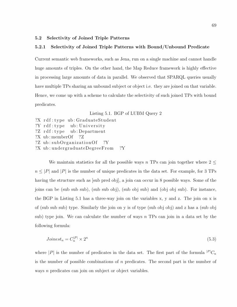
69
5.2 Selectivity of Joined Triple Patterns
5.2.1 Selectivity of Joined Triple Patterns with Bound/Unbound Predicate
Current semantic web frameworks, such as Jena, run on a single machine and cannot handle
huge amounts of triples. On the other hand, the Map Reduce framework is highly effective
in processing large amounts of data in parallel. We observed that SPARQL queries usually
have multiple TPs sharing an unbound subject or object i.e. they are joined on that variable.
Hence, we come up with a scheme to calculate the selectivity of such joined TPs with bound
predicates.
Listing 5.1. BGP of LUBM Query 2
?X rd f : type ub : GraduateStudent?Y rd f : type ub : Un ive r s i ty?Z rd f : type ub : Department?X ub : memberOf ?Z?Z ub : subOrganizat ionOf ?Y?X ub : undergraduateDegreeFrom ?Y
We maintain statistics for all the possible ways n TPs can join together where 2 ≤
n ≤ |P | and |P | is the number of unique predicates in the data set. For example, for 3 TPs
having the structure such as [sub pred obj], a join can occur in 8 possible ways. Some of the
joins can be (sub sub sub), (sub sub obj), (sub obj sub) and (obj obj sub). For instance,
the BGP in Listing 5.1 has a three-way join on the variables x, y and z. The join on x is
of (sub sub sub) type. Similarly the join on y is of type (sub obj obj) and z has a (sub obj
sub) type join. We can calculate the number of ways n TPs can join in a data set by the
following formula:
Joinestn = C |P |n × 2n (5.3)
where |P | is the number of predicates in the data set. The first part of the formula |P |Cn
is the number of possible combinations of n predicates. The second part is the number of
ways n predicates can join on subject or object variables.
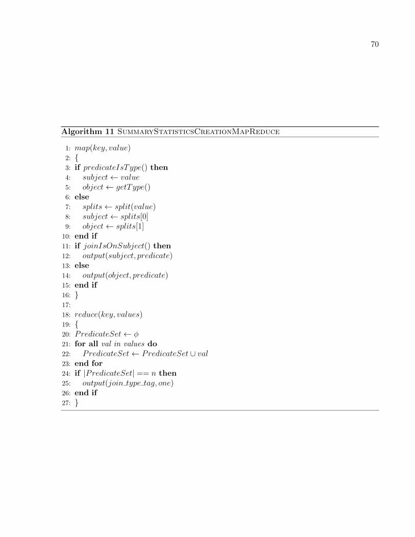
70
Algorithm 11 SummaryStatisticsCreationMapReduce
1: map(key, value)2: {3: if predicateIsType() then4: subject← value5: object← getType()6: else7: splits← split(value)8: subject← splits[0]9: object← splits[1]10: end if11: if joinIsOnSubject() then12: output(subject, predicate)13: else14: output(object, predicate)15: end if16: }17:
18: reduce(key, values)19: {20: PredicateSet← φ21: for all val in values do22: PredicateSet← PredicateSet ∪ val23: end for24: if |PredicateSet| == n then25: output(join type tag, one)26: end if27: }
71
In the summary statistics, we maintain a separate count for all such n-ary joins where
2 ≤ n ≤ |P |. This helps us estimate the selectivity of a joined triple pattern. Gathering the
statistics requires vast amount of memory. A program running on a single machine runs out
of memory while generating the statistics. So, we run Hadoop MapReduce jobs to collect
them. In the map phase, we read a file one line at a time and split it to get the subject
and object. From the file name we have the predicate. Based on what type of join we are
considering, we output either the subject or the object as the key. The value is always the
predicate. Algorithm 11 shows our map method in lines 1 to 16. In line 3, it checks whether
the input file is of predicate type. In such a case, subject is the value which is a single string
and the object is the type of the subject which is determined from the file name. If the input
file is not for predicate type, we split the value string into two strings in line 7. In line 8 and
9, we get the subject and the object. In line 11, we check if the join is on subject. If that is
the case, we output subject as the key and predicate as the value in line 12. Otherwise, in
line 13, we output object as the key and predicate as the value. In the reduce phase, for each
key we count the number of unique predicates. If that equals to n, we output an integer 1.
Algorithm 11 shows our reduce method in lines 18 to 27. In line 20, we initialize a set which
we use to hold the unique predicates. In line 21, we iterate over each value in a for loop and
in line 22 we insert the predicate in the set. Note that, as the set only hold unique values,
it will not include any duplicate value in line 22. In line 24, we compare the size of the set
with n. If they are equal, we output a string, describing the join type, as the key and an
integer 1 as the value in line 25. The string identifying the join contains information about
the predicates and join type.
We use another job to sum up these 1’s to get the total count. Algorithm 12 shows
the map method for that job from lines 1 to 5. The method simply parses each line and
splits it into two in line 3. In line 4, it outputs the first split as the key and the second split
as the value. Hence, the key is the id for join type and value is 1. Algorithm 12 show the
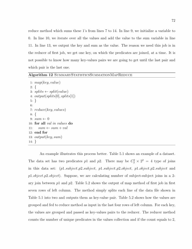
72
reduce method which sums these 1’s from lines 7 to 14. In line 9, we initialize a variable to
0. In line 10, we iterate over all the values and add the value to the sum variable in line
11. In line 13, we output the key and sum as the value. The reason we need this job is in
the reducer of first job, we get one key, on which the predicates are joined, at a time. It is
not possible to know how many key-values pairs we are going to get until the last pair and
which pair is the last one.
Algorithm 12 SummaryStatisticsSummationMapReduce
1: map(key, value)2: {3: splits← split(value)4: output(splits[0], splits[1])5: }6:
7: reduce(key, values)8: {9: sum← 010: for all val in values do11: sum← sum+ val12: end for13: output(key, sum)14: }
An example illustrates this process better. Table 5.1 shows an example of a dataset.
The data set has two predicates p1 and p2. There may be C22 × 22 = 4 type of joins
in this data set: (p1 subject p2 subject, p1 subject p2 object, p1 object p2 subject and
p1 object p2 object). Suppose, we are calculating number of subject-subject joins in a 2-
ary join between p1 and p2. Table 5.2 shows the output of map method of first job in first
seven rows of left column. The method simply splits each line of the data file shown in
Table 5.1 into two and outputs them as key-value pair. Table 5.2 shows how the values are
grouped and fed to reduce method as input in the last four rows of left column. For each key,
the values are grouped and passed as key-values pairs to the reducer. The reducer method
counts the number of unique predicates in the values collection and if the count equals to 2,
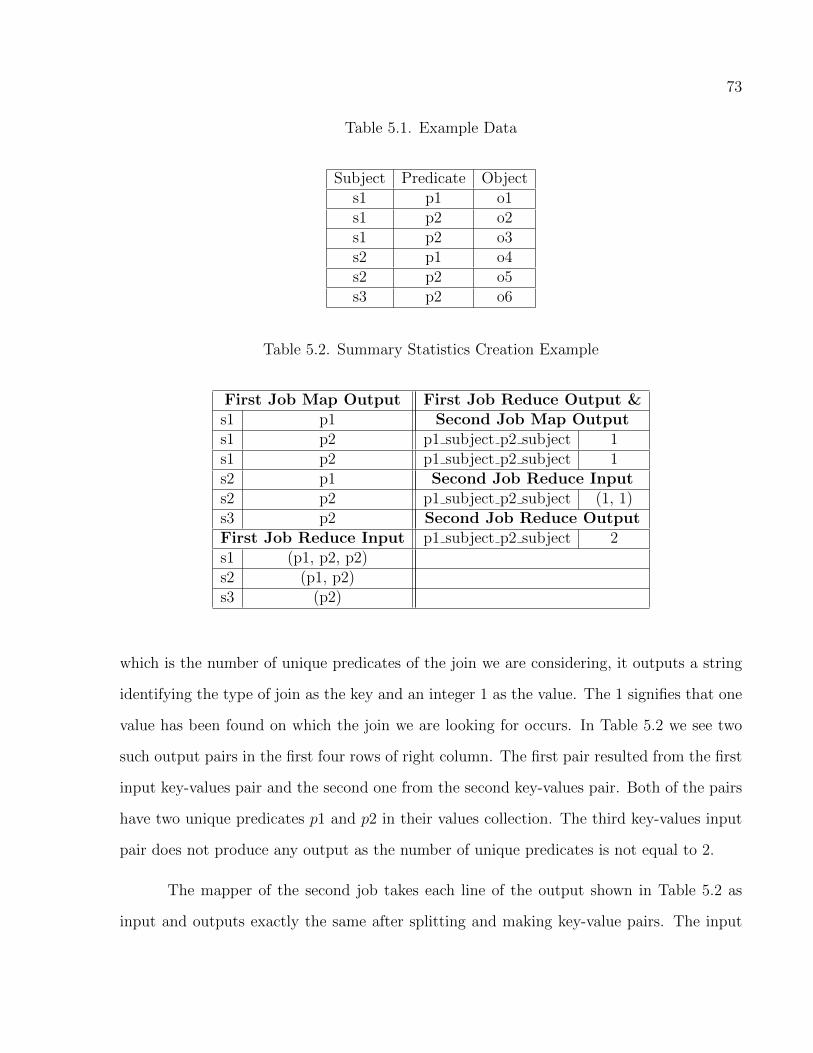
73
Table 5.1. Example Data
Subject Predicate Objects1 p1 o1s1 p2 o2s1 p2 o3s2 p1 o4s2 p2 o5s3 p2 o6
Table 5.2. Summary Statistics Creation Example
First Job Map Output First Job Reduce Output &s1 p1 Second Job Map Outputs1 p2 p1 subject p2 subject 1s1 p2 p1 subject p2 subject 1s2 p1 Second Job Reduce Inputs2 p2 p1 subject p2 subject (1, 1)s3 p2 Second Job Reduce OutputFirst Job Reduce Input p1 subject p2 subject 2s1 (p1, p2, p2)s2 (p1, p2)s3 (p2)
which is the number of unique predicates of the join we are considering, it outputs a string
identifying the type of join as the key and an integer 1 as the value. The 1 signifies that one
value has been found on which the join we are looking for occurs. In Table 5.2 we see two
such output pairs in the first four rows of right column. The first pair resulted from the first
input key-values pair and the second one from the second key-values pair. Both of the pairs
have two unique predicates p1 and p2 in their values collection. The third key-values input
pair does not produce any output as the number of unique predicates is not equal to 2.
The mapper of the second job takes each line of the output shown in Table 5.2 as
input and outputs exactly the same after splitting and making key-value pairs. The input

74
the reducer gets is shown in Table 5.2 in 5th and 6th rows of right column. It sums up the
1’s and outputs the key and the sum as the value. The output is shown in Table 5.2 in 7th
and 8th rows of right column. Thus, we get the number of subject-subject joins for 2-way
join between p1 and p2.
CHAPTER 6
RESULTS
In this chapter, we will present our experimental results. First, we present the bench-
mark data sets with which we experimented. Second, we present the alternative repositories
we evaluated for comparison. Third, we detail our experimental setup. Finally, we present
our evaluation results.
6.1 Data Sets
In our experiments with SPARQL query processing, we use two synthetic data sets:
LUBM(Guo, Pan, and Heflin 2005) and SP2B(Schmidt, Hornung, Lausen, and Pinkel 2008).
The LUBM data set generates data about universities by using an ontology†. It has 14
standard queries. Some of the queries require inference to answer. The LUBM data set is
very good for both inference and scalability testing. For all LUBM data sets, we used the
default seed. The SP2B data set is good for scalability testing with complex queries and
data access patterns. It has 16 queries most of which have complex structures.
6.2 Baseline Frameworks
We compared our framework with RDF-3X(Neumann and Weikum 2008), Jena† and
BigOWLIM†. RDF-3X is considered the fastest semantic web framework with persistent
storage. Jena is an open source framework for semantic web data. It has several models
†http://www.lehigh.edu/~zhp2/2004/0401/univ-bench.owl†http://jena.sourceforge.net†http://www.ontotext.com/owlim/big/index.html
75
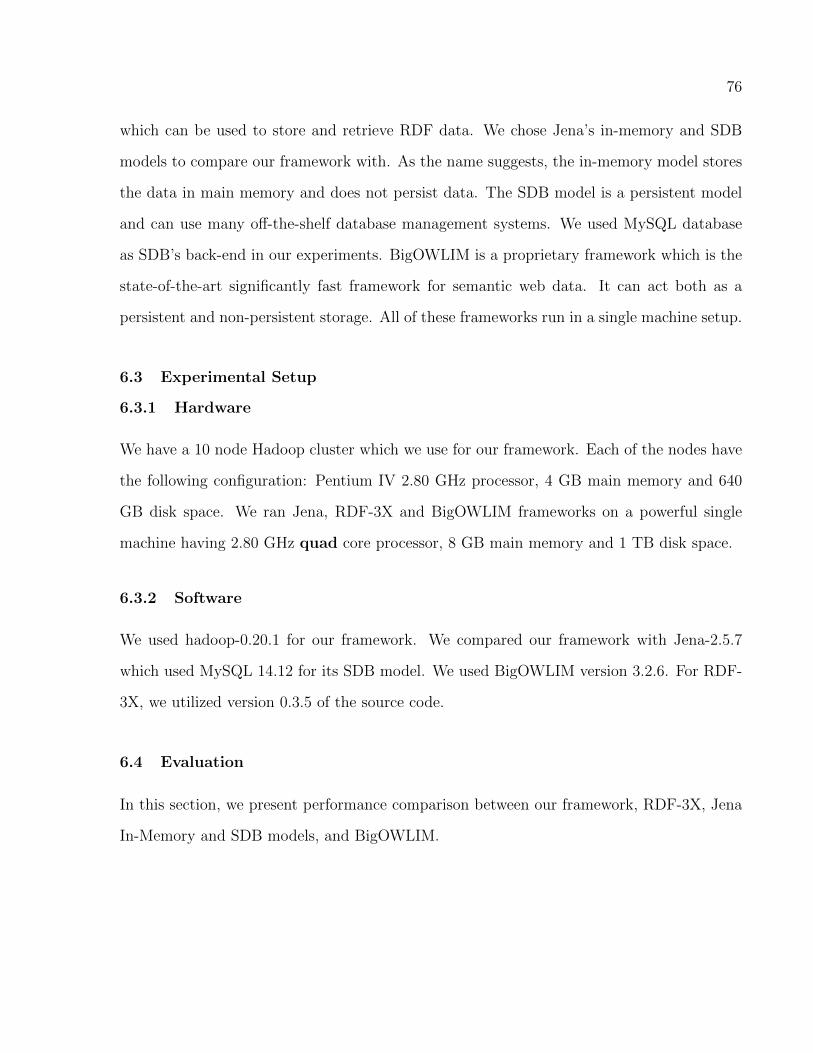
76
which can be used to store and retrieve RDF data. We chose Jena’s in-memory and SDB
models to compare our framework with. As the name suggests, the in-memory model stores
the data in main memory and does not persist data. The SDB model is a persistent model
and can use many off-the-shelf database management systems. We used MySQL database
as SDB’s back-end in our experiments. BigOWLIM is a proprietary framework which is the
state-of-the-art significantly fast framework for semantic web data. It can act both as a
persistent and non-persistent storage. All of these frameworks run in a single machine setup.
6.3 Experimental Setup
6.3.1 Hardware
We have a 10 node Hadoop cluster which we use for our framework. Each of the nodes have
the following configuration: Pentium IV 2.80 GHz processor, 4 GB main memory and 640
GB disk space. We ran Jena, RDF-3X and BigOWLIM frameworks on a powerful single
machine having 2.80 GHz quad core processor, 8 GB main memory and 1 TB disk space.
6.3.2 Software
We used hadoop-0.20.1 for our framework. We compared our framework with Jena-2.5.7
which used MySQL 14.12 for its SDB model. We used BigOWLIM version 3.2.6. For RDF-
3X, we utilized version 0.3.5 of the source code.
6.4 Evaluation
In this section, we present performance comparison between our framework, RDF-3X, Jena
In-Memory and SDB models, and BigOWLIM.
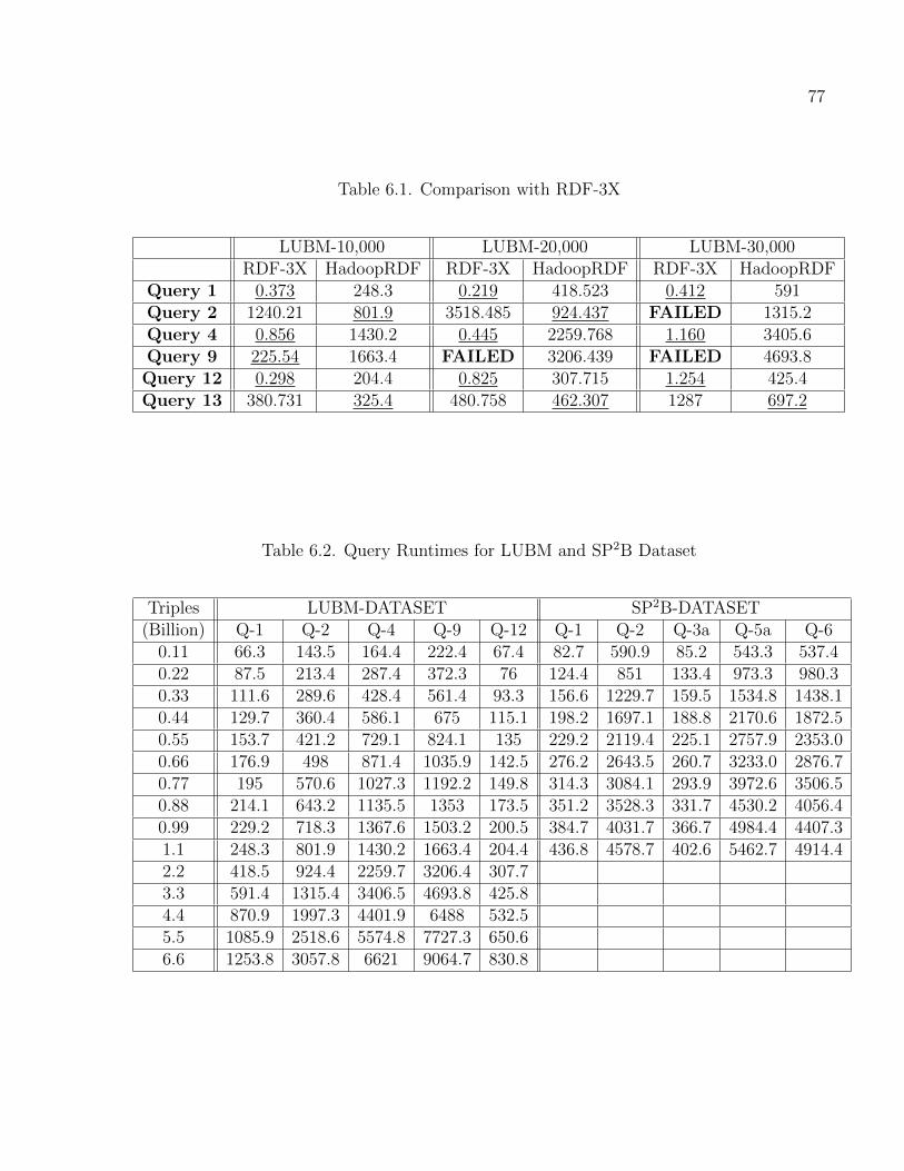
77
Table 6.1. Comparison with RDF-3X
LUBM-10,000 LUBM-20,000 LUBM-30,000RDF-3X HadoopRDF RDF-3X HadoopRDF RDF-3X HadoopRDF
Query 1 0.373 248.3 0.219 418.523 0.412 591Query 2 1240.21 801.9 3518.485 924.437 FAILED 1315.2Query 4 0.856 1430.2 0.445 2259.768 1.160 3405.6Query 9 225.54 1663.4 FAILED 3206.439 FAILED 4693.8Query 12 0.298 204.4 0.825 307.715 1.254 425.4Query 13 380.731 325.4 480.758 462.307 1287 697.2
Table 6.2. Query Runtimes for LUBM and SP2B Dataset
Triples LUBM-DATASET SP2B-DATASET(Billion) Q-1 Q-2 Q-4 Q-9 Q-12 Q-1 Q-2 Q-3a Q-5a Q-6
0.11 66.3 143.5 164.4 222.4 67.4 82.7 590.9 85.2 543.3 537.40.22 87.5 213.4 287.4 372.3 76 124.4 851 133.4 973.3 980.30.33 111.6 289.6 428.4 561.4 93.3 156.6 1229.7 159.5 1534.8 1438.10.44 129.7 360.4 586.1 675 115.1 198.2 1697.1 188.8 2170.6 1872.50.55 153.7 421.2 729.1 824.1 135 229.2 2119.4 225.1 2757.9 2353.00.66 176.9 498 871.4 1035.9 142.5 276.2 2643.5 260.7 3233.0 2876.70.77 195 570.6 1027.3 1192.2 149.8 314.3 3084.1 293.9 3972.6 3506.50.88 214.1 643.2 1135.5 1353 173.5 351.2 3528.3 331.7 4530.2 4056.40.99 229.2 718.3 1367.6 1503.2 200.5 384.7 4031.7 366.7 4984.4 4407.31.1 248.3 801.9 1430.2 1663.4 204.4 436.8 4578.7 402.6 5462.7 4914.42.2 418.5 924.4 2259.7 3206.4 307.73.3 591.4 1315.4 3406.5 4693.8 425.84.4 870.9 1997.3 4401.9 6488 532.55.5 1085.9 2518.6 5574.8 7727.3 650.66.6 1253.8 3057.8 6621 9064.7 830.8
78
6.4.1 Comparison with Baseline Frameworks
Table 6.1 summarizes our comparison with RDF-3X. We used three LUBM datasets: 10,000,
20,000 and 30,000 which have more than 1.1, 2.2 and 3.3 billion triples respectively. Inital
population time for RDF-3X took 655 minutes, 1756 minutes, and 3353 minutes to load the
datasets respectively. This shows that the RDF-3X load time is increasing exponentionally.
LUBM(30,000) has 3 times as many triples as LUBM(10,000) yet it requires more than 5
times as long to load.
For evaluations purposes, we chose LUBM Queries 1, 2, 4, 9, 12 and 13 to be re-
ported in this paper. These queries provide a good mixture and include simple and complex
structures, inference and multiple types of joins. They are representatives of other queries
of the benchmark and so reporting only these covers all types of variations found in the
queries we left out and also saves space. Query 1 is a simple selective query. RDF-3X is
much faster than HadoopRDF for this query. RDF-3X utilizes six indexes (Neumann and
Weikum 2008) and those six indexes actually make up the data set. The indexes provide
RDF-3X a very fast way to look up triples, similar to a hash table. Hence, a highly selective
query is efficiently answered by RDF-3X. Query 2 is a query with complex structures, low
selectivity and no bound objects. The result set is quite large. For this query, HadoopRDF
outperforms RDF-3X for all 3 dataset sizes. RDF-3X fails to answer the query at all when
the dataset size is 3.3 billion triples. RDF-3X returns a memory segmentation fault error
messages, and does not produce any query results. Query 4 is also a highly selective query
i.e. the result set size is small because of a bound object in the second triple pattern but
it needs inferencing to answer it. The first triple pattern uses the class Person which is a
superclass of many classes. No resource in LUBM dataset is of type Person, rather there
are many resources which are its sub-types. RDF-3X does not support inferencing so we
had to convert the query to an equivalent query having some union operations. RDF-3X
outperforms HadoopRDF for this query. Query 9 is similar in structure to Query 2 but it
79
requires significant inferencing. The first three triple patterns of this query uses classes of
which are not explicitly instantiated in the dataset. However, the dataset includes many
instances of the corresponding subclasses. This is also the query which requires the largest
dataset join and returns the largest result set out of the queries we evaluated. RDF-3X is
faster than HadoopRDF for 1.1 billion triples dataset but it fails to answer the query at all
for the other two datasets. Query 12 is similar to Query 4 because it is both selective and
has inferencing in one triple pattern. RDF-3X beats HadoopRDF for this query. Query 13
has only two triple patterns. Both of them involve inferencing. There is a bound subject in
the 2nd triple pattern. It returns the second largest result set. HadoopRDF beats RDF-3X
for this query for all datasets. RDF-3X’s performance is slow because the first triple pattern
has very low selectivity and requires low selectivity joins to perform inference via backwards
chaining.
These results lead us to some simple conclusions. RDF-3X achieves the best per-
formance for queries with high selectivity and bound objects. However, HadoopRDF out-
performs RDF-3X for queries with unbound objects, low selectivity, or large dataset joins.
RDF-3X cannot execute the two queries with unbound objects (Query 2 and 9) for a 3.3
billion triples dataset. This demonstrates that HadoopRDF is more scalable and handles
low selectivity queries more efficiently than RDF-3X.
We also compared our implementation with the Jena In-Memory model and the SDB
models and BigOWLIM. Due to space and time limitations, we performed these tests only
for LUBM Queries 2 and 9 from the LUBM dataset. We chose these queries because they
have complex structures and require inference. It is to be noted that BigOWLIM needed 7
GB of Java heap space to successfully load the billion triples dataset. Figures 6.1 and 6.2
show the performance comparison for the queries respectively. In each of these figures, the
X axis represents the number of triples (in billions) and the Y axis represents the time (in
seconds). We ran BigOWLIM only for the largest three datasets as we are interested in its
80
performance with large datasets. For each set, on the X axis, there are four columns which
show the results of Jena In-Memory model, Jena SDB model, our Hadoop implementation
and BigOWLIM respectively. A cross represents either that the query could not complete or
that it ran out of memory. In most of the cases, our approach was the fastest. For Query 2,
Jena In-Memory Model and Jena SDB model were faster than our approach, giving results in
3.9 and 0.4 seconds respectively. However, as the size of the dataset grew, Jena In-Memory
model ran out of memory space. Our implementation was much faster than Jena SDB model
for large datasets. For example, in Figure 6.1 for 110 million triples, our approach took 143.5
seconds as compared to about 5000 seconds for Jena-SDB model. In Figure 6.2, we can see
that Jena SDB model could not finish answering Query 9. Jena In-Memory Model worked
well for small datasets but became slower than our implementation as the dataset size grew
and eventually ran out of memory. For Query 2 (Figure 6.1), BigOWLIM was slower than us
for the 110 and 550 million datasets. For 550 million dataset it took 22693.4 seconds, which
is abruptly high compared to its other timings. For the billion triple dataset, BigOWLIM
was faster. It should be noted that our framework does not have any indexing or triple cache
whereas BigOWLIM exploits indexing which it loads into main memory when it starts. It
may also pre-fetch triples into main memory. For Query 9 (Figure 6.2), our implementation
is faster than BigOWLIM in all experiments.
It should be noted that our RDF-3X queries and HadoopRDF queries were tested
using cold runs. What we mean by this is that main memory and file system cache were
cleared prior to execution. However, for BigOWLIM, we were forced to execute hot runs.
This is because it takes a significant amount of time to load a database into BigOWLIM.
Therefore, we will always easily outperform BigOWLIM for cold runs. So we actually tested
BigOWLIM for hot runs against HadoopRDF for cold runs. This gives a tremendous advan-
tage to BigOWLIM, yet for large datasets HadoopRDF still produced much better results.
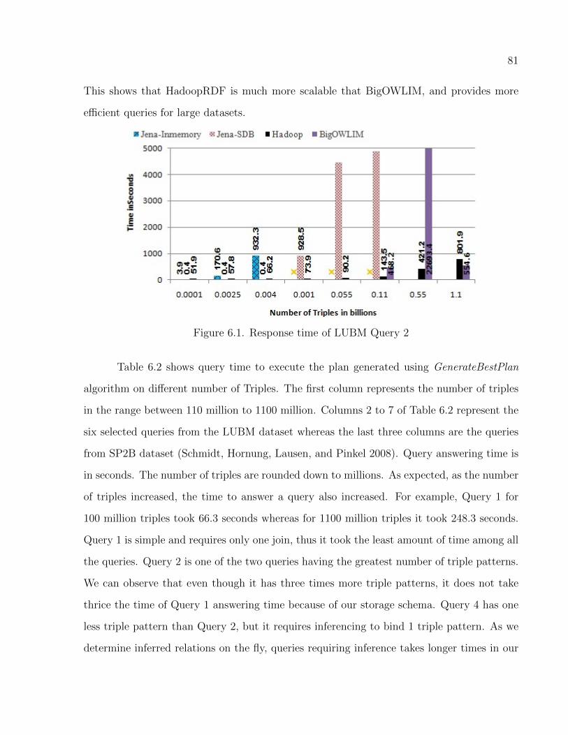
81
This shows that HadoopRDF is much more scalable that BigOWLIM, and provides more
efficient queries for large datasets.
Figure 6.1. Response time of LUBM Query 2
Table 6.2 shows query time to execute the plan generated using GenerateBestPlan
algorithm on different number of Triples. The first column represents the number of triples
in the range between 110 million to 1100 million. Columns 2 to 7 of Table 6.2 represent the
six selected queries from the LUBM dataset whereas the last three columns are the queries
from SP2B dataset (Schmidt, Hornung, Lausen, and Pinkel 2008). Query answering time is
in seconds. The number of triples are rounded down to millions. As expected, as the number
of triples increased, the time to answer a query also increased. For example, Query 1 for
100 million triples took 66.3 seconds whereas for 1100 million triples it took 248.3 seconds.
Query 1 is simple and requires only one join, thus it took the least amount of time among all
the queries. Query 2 is one of the two queries having the greatest number of triple patterns.
We can observe that even though it has three times more triple patterns, it does not take
thrice the time of Query 1 answering time because of our storage schema. Query 4 has one
less triple pattern than Query 2, but it requires inferencing to bind 1 triple pattern. As we
determine inferred relations on the fly, queries requiring inference takes longer times in our
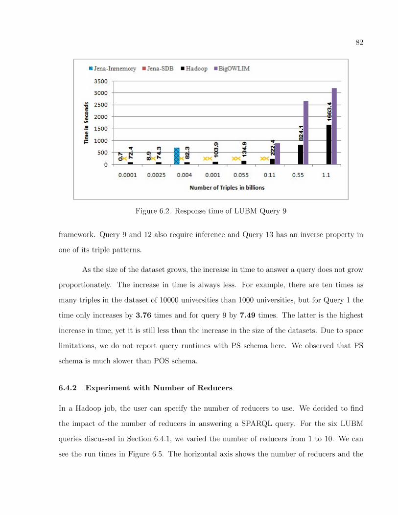
82
Figure 6.2. Response time of LUBM Query 9
framework. Query 9 and 12 also require inference and Query 13 has an inverse property in
one of its triple patterns.
As the size of the dataset grows, the increase in time to answer a query does not grow
proportionately. The increase in time is always less. For example, there are ten times as
many triples in the dataset of 10000 universities than 1000 universities, but for Query 1 the
time only increases by 3.76 times and for query 9 by 7.49 times. The latter is the highest
increase in time, yet it is still less than the increase in the size of the datasets. Due to space
limitations, we do not report query runtimes with PS schema here. We observed that PS
schema is much slower than POS schema.
6.4.2 Experiment with Number of Reducers
In a Hadoop job, the user can specify the number of reducers to use. We decided to find
the impact of the number of reducers in answering a SPARQL query. For the six LUBM
queries discussed in Section 6.4.1, we varied the number of reducers from 1 to 10. We can
see the run times in Figure 6.5. The horizontal axis shows the number of reducers and the
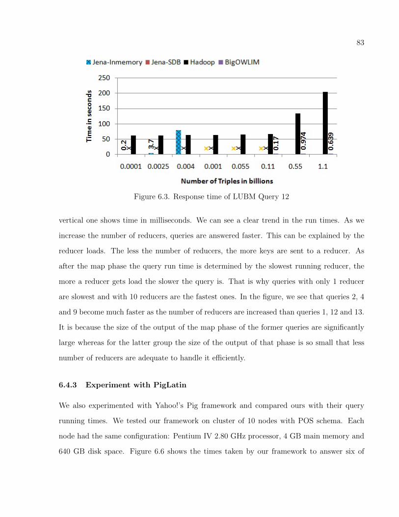
83
Figure 6.3. Response time of LUBM Query 12
vertical one shows time in milliseconds. We can see a clear trend in the run times. As we
increase the number of reducers, queries are answered faster. This can be explained by the
reducer loads. The less the number of reducers, the more keys are sent to a reducer. As
after the map phase the query run time is determined by the slowest running reducer, the
more a reducer gets load the slower the query is. That is why queries with only 1 reducer
are slowest and with 10 reducers are the fastest ones. In the figure, we see that queries 2, 4
and 9 become much faster as the number of reducers are increased than queries 1, 12 and 13.
It is because the size of the output of the map phase of the former queries are significantly
large whereas for the latter group the size of the output of that phase is so small that less
number of reducers are adequate to handle it efficiently.
6.4.3 Experiment with PigLatin
We also experimented with Yahoo!’s Pig framework and compared ours with their query
running times. We tested our framework on cluster of 10 nodes with POS schema. Each
node had the same configuration: Pentium IV 2.80 GHz processor, 4 GB main memory and
640 GB disk space. Figure 6.6 shows the times taken by our framework to answer six of
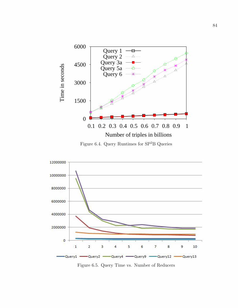
84
0
1500
3000
4500
6000
0.1 0.2 0.3 0.4 0.5 0.6 0.7 0.8 0.9 1
Tim
e in
sec
onds
Number of triples in billions
Query 1Query 2
Query 3aQuery 5aQuery 6
Figure 6.4. Query Runtimes for SP2B Queries
Figure 6.5. Query Time vs. Number of Reducers
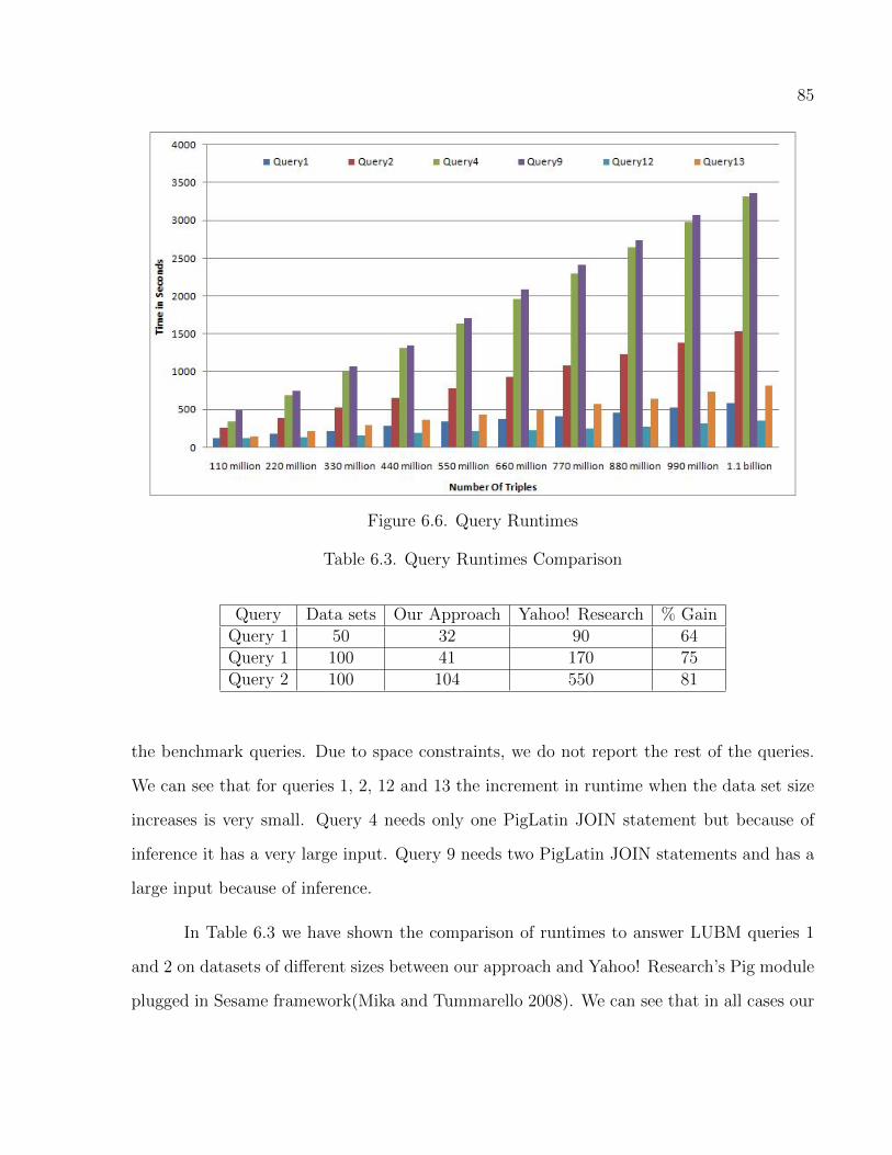
85
Figure 6.6. Query Runtimes
Table 6.3. Query Runtimes Comparison
Query Data sets Our Approach Yahoo! Research % GainQuery 1 50 32 90 64Query 1 100 41 170 75Query 2 100 104 550 81
the benchmark queries. Due to space constraints, we do not report the rest of the queries.
We can see that for queries 1, 2, 12 and 13 the increment in runtime when the data set size
increases is very small. Query 4 needs only one PigLatin JOIN statement but because of
inference it has a very large input. Query 9 needs two PigLatin JOIN statements and has a
large input because of inference.
In Table 6.3 we have shown the comparison of runtimes to answer LUBM queries 1
and 2 on datasets of different sizes between our approach and Yahoo! Research’s Pig module
plugged in Sesame framework(Mika and Tummarello 2008). We can see that in all cases our
86
framework performed much better than theirs. For query 1 on data set of 50 universities, we
are 64% faster. For the same query on data set of 100 universities, we are 75% faster, which
indicates that as the size of the data set grows, our framework performs even more better.
For query 2 on same data set we have the highest gain.
We note that Figure 1 of (Mika and Tummarello 2008), for 10 node cluster query exe-
cution time for LUBM query 1 on 1000 universities dataset is not shown as it is much higher
than 600 seconds which is the maximum runtime shown in the graph. In our experiments,
we took 248.3 seconds to answer the same query which is substantially less than even 600
seconds.
6.5 Validation
We validated our results returned by our framework by comparing with the results returned
by other ones. For small data sets, we used Jena in-memory and SDB models. For large
data set, we compared with the numbers of BigOWLIM for LUBM 8000 data set reported at
http://www.ontotext.com/owlim/benchmark-results/lubm. To automate the process,
we used Java programs to validate the results.
CHAPTER 7
ACCESS CONTROL
The presently used RDF stores aren’t too concerned with implementing security in
them. Efforts have been put in to incorporate security, especially in Jena (Reddivari, Finin,
and Joshi 2005; Jain and Farkas 2006). The drawback with Jena is that it lacks scalability.
As to our knowledge, access control hasn’t been implemented on RDF stores in Hadoop and
we are the first ones to propose it. In this chapter, we present our proposed system which
implements a token based access control system. Access tokens are issued for some portion
of data for issuing access. The system administrator grants tokens along with the granting
time stamps to agents according to agents’ need and security levels. Conflicts might arise
due to an agents’ undue data access. Time stamps are used to resolve conflicts. We are using
LUBM (Guo, Pan, and Heflin 2005) test instances for experiments. A few sample scenarios
have been generated and implemented in Hadoop. Although tokens have been used by others
for access control to manage XML(Bouganim, Ngoc, and Pucheral 2004) documents, Digital
Information(Holmquist, Redstrom, and Ljungstrand 1999), they have not been used for RDF
stores. One of the advantages of using tokens is that they can be reused if the needs and
security requirements for more than one agents are the same.
We have several contributions. First, we are proposing an architecture that addresses
scalability. Second, we are addressing access control not only on user levels but also on
subject, object, and predicate levels – making it more granular. Third, a time stamp based
conflict detection and resolution algorithm has been proposed. Fourth, the architecture has
been implemented and tested on benchmark data set in several alternative stages – Query
87
88
Rewriting (pre processing phase), Embedded Enforcement (MapReduce execution phase),
and Post-processing Enforcement (data displaying phase). Finally, the whole system is
being implemented on Hadoop – a open source cloud computing environment. We believe
that this work is going to be beneficial for others considering access control for RDF data in
Hadoop.
The remainder of the chapter is organized as follows. In Section 7.1, we introduce
Access Tokens, Access Token Tuples, conflicts, and conflict resolution algorithm. We describe
the modified architecture of the our system in Section 7.2. The experiments and their run
times are included in Section 7.4.
7.1 Access Control Level Descriptions
Definition 1. Access Tokens (AT): An Access Token (AT) can be generated on some par-
ticular data. If an agent is in possession of an AT then she can view the data permitted by
that AT. We are denoting ATs with numbers. For example, 1, 2, 3, etc. The system stores
the tokens itself.
Definition 2. Access Token Tuple(ATT): Access Token Tuples (ATT) are of the form
〈AccessToken,Element, ElementType, ElementName〉. The Element can be Subject,
Object, or Predicate. ElementType can be described as URI, DataType, Literal, Model,
or BlankNode. Model is only used while accessing Subjects for accessing Subject Models.
The usage of it will be explained in detail later on. ElementName is the name of the
Element.
For example, David is a subject in figure 7.2 and 〈1, Subject, URI,David〉 is an ATT.
Here 1, Subject, and David represents AccessToken, ElementType, and Elementname
respectively. Any agent having this security level, 1, can retrieve David’s information over all
the files considering that she doesn’t have other security restrictions viewing URIs, literals,
89
etc. associate with David’s objects. While describing ATs for Predicates we leave the
ElementName blank ( ).
Based on the record organization six types Access Levels along with a few sub types.
An agent can be assigned one of the following access levels or a combination or a more
restricted version of them.
1. Predicate’s Data Access: In an access level if an object type is defined for one par-
ticular predicate then an agent having that access level can read the whole predicate
file considering the agent has the tokens to access sensitive subject and object informa-
tion, if there exists any sensitive information. For example, 〈1 , P redicate, isPaid, 〉 is
an ATT. If an agent is presented with 1 access token without other restrictions, she
can read the whole predicate file isPaid.
2. Predicate, and Subjects’ Data Access: This is one of the most restrictive access
levels. Here the Subject can be either an URI, or a Data Type. For simplicity, we are
not considering subjects to be blank nodes currently.
(a) Predicate, and Subject as an URI: Here, a specific subject’s information
retrieved over a predicate file. As an example, agent X has an access ticket of
1. With access ticket 1, X can access one subject with URI MichaelScott of
Predicate isPaid. This scenario can be represented by 〈1 , predicate, isPaid, 〉
and 〈1 , subject,MichealScott, URI〉 tuples (displayed in Figure 7.2).
(b) Predicate, and Subject as a Data Type: As the title suggests, the informa-
tion of the subjects of a specific data type over a predicate file will be retrieved.
For brevity, we are not going to explain the subject or object sub divisions in detail
from this moment on.
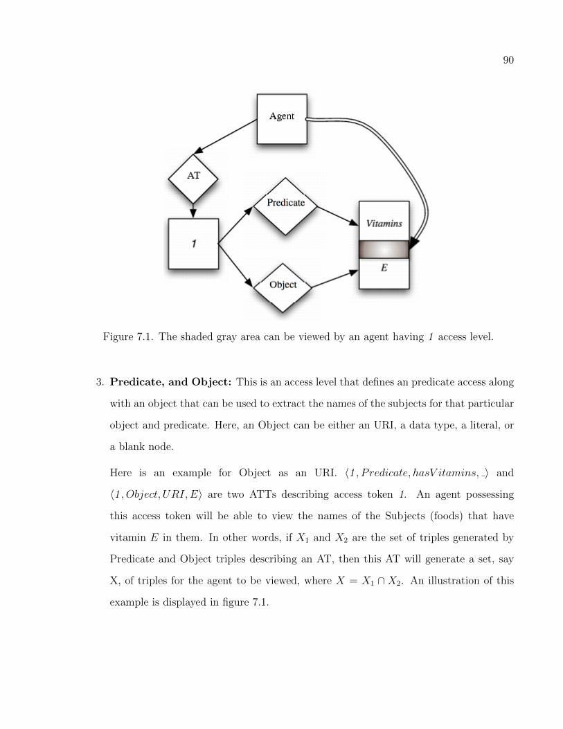
90
Figure 7.1. The shaded gray area can be viewed by an agent having 1 access level.
3. Predicate, and Object: This is an access level that defines an predicate access along
with an object that can be used to extract the names of the subjects for that particular
object and predicate. Here, an Object can be either an URI, a data type, a literal, or
a blank node.
Here is an example for Object as an URI. 〈1 , P redicate, hasV itamins, 〉 and
〈1 , Object, URI,E〉 are two ATTs describing access token 1. An agent possessing
this access token will be able to view the names of the Subjects (foods) that have
vitamin E in them. In other words, if X1 and X2 are the set of triples generated by
Predicate and Object triples describing an AT, then this AT will generate a set, say
X, of triples for the agent to be viewed, where X = X1 ∩ X2. An illustration of this
example is displayed in figure 7.1.

91
4. Subject Access: With this access level one can read the subjects information over
all the files. This is one of the less restrictive access levels. The subject can be either
an URI, a Data type, or a blank node.
5. Object Access: With this access level one can read the objects subjects over all the
files. Like the last one, this is one of the less restrictive access levels. As previously
mentioned, an Object can be either of these – an URI, a data type, a literal, or a blank
node.
6. Subject Model Level Access: In this case, for one subject, an agent will read all the
necessary predicate files to obtain its objects. Of these objects, the ones that are URIs,
are treated as subjects for the next step to extract their information (predicates and
objects). This recursive process of extracting objects of subjects and treating URIs of
objects as subjects for the next round continues until all objects finally become literals
or blank nodes. In this manner, an agent can generate models on a subject if she has
Subject Model level access.
Let’s illustrate this with an example from figure 1. David lives in Long Island city.
Since LongIsland city has can be a Subject with Ave Summer Temp (Average Summer
Temperature) Predicate, its Object (75F ) will be retrieved as well. Having Model
Level Access of David guarantees that one would be able to see the average summer
temperature of Long Island.
7.1.1 Access Token Assignment
Definition 3. Access Token List (AT-list): For each qualified agent an AT-list is maintained.
An AT-list is an array composed of one or more ATs along with the granting time stamp of
each AT to that agent.
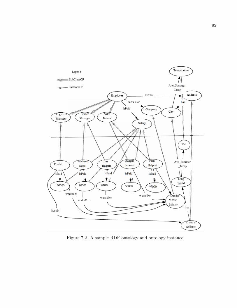
92
Figure 7.2. A sample RDF ontology and ontology instance.
93
Once it is decided by the system administrator that an AT will be added to an agent’s
AT-list, the administrator stores the AT along with the time stamp in a temporary variable
TempAT of type AT. It is checked then whether TempAT could be added to this agent’s
AT-list without any conflict.
7.1.2 Final output of an Agent’s ATs
Each AT for an agent will return a set of triples. If the there are more than one ATs
assigned to an agent then the final sets of triples is going to be the union of the sets of triples
returned by each AT in his AT-list. Formally, if Y1, Y2, ...., Yn are the set of triples returned
by AT1, AT2, .... , ATn respectively in an agent’s AT-list and Yfinal set of output triples then
Yfinal = Y1 ∪ Y2 ∪ .... ∪ Yn (7.1)
7.1.3 Assumptions
1. Each item in the data store has a default security level.
2. A person’s identity and information is kept private by system by default. Any URI of
data type person is inaccessible and kept hidden unless explicitly specified in the ATs.
It will prevent making inferences about a person that the agent doesn’t have access to.
Here is an example. Consider a predicate file Likes where the elements that a per-
son likes are listed. So, if Jim is a person and he likes Flying, Semantic Web,
and Jenny where as Flying, Semantic Web, and Jenny are the URIs of types
Hobby, Research Interest, and Person respectively. 1 is an AT with ATTs 〈1
, Subject, URI, Jim〉, and 〈1 , Likes, Predicate , 〉. Anyone, say, Ben just having
AT 1 won’t be able to know that Jenny is in Jim’s like-list since Jenny’s data type
is person. Then again, if Ben has an access token 2 where 2 is described with 〈2,
Object, URI, Jenny〉 ATT then Ben will be able to see Jenny in Jim’s like-list.

94
3. If an agent has access to a particular type or property, she will have implicit access to
the subtypes or sub-properties of that type or property.
7.1.4 Conflicts
A conflict arises when the following three conditions occur. An agent possesses two or more
ATs, the result set of one of the ATs is a proper subset of another AT, and the time stamp
of the larger set is smaller than the time stamp of the smaller one.
There could be situations when an agent might end up having more access to a data
store than she is supposed to have. These situations need to be detected and prevented.
The algorithms for conflict detection and resolution are stated later. In case there arises a
conflict time stamps will be used to resolve it. If two ATs are conflicting then the their time
stamps (TS) will be used to resolve the conflict.
7.1.4.1 Subset Conflict
If there are two ATs and the result set of one ATs is a proper subset of the other one
then this conflict arises if the time stamp of the smaller set is greater than the time stamp
of the larger set. Examining whether triples generated by a newly added AT is a subset
triples generated of another AT can be performed by looking at their ATTs. For example,
1 and 2 are two ATs. 〈1 , Subject, URI, Sam〉, and 〈2, Subject, URI, Sam〉, and
〈2, Predicate, HasAccounts, 〉 ATTs describe 1 and 2 respectively. Naturally, triples
returned by 2 will be a subset of triples returned by 1. A conflict will occur when anyone
possessing 1 is assigned 2 with a larger time stamp. So, 1 will be removed from her AT-list
to resolve this conflict.
7.1.4.2 SubType Conflict
This conflict arises because of two reasons.

95
Due to Subject For any two ATs for an agent, if the data type of subject in one of the
ATs is subtype of the data type of the other AT then and the time stamp of the former
AT is larger than the later one, then this conflict arises. The AT with the super data
type is removed from an agent’s AT-list.
Due to Object Over here, instead of Subject, the conflict arises due to Object URIs and
Types.
7.1.4.3 Conflict Resolution
As mentioned earlier, conflicts can arise during the assignment of an AT. For the sake of
brevity, we don’t show all of the places where conflicts can arise in the Conflict Detection
and Resolution algorithm. We only show the places where the existing ATs are replaced.
The formal description of detecting conflicts and resolving them is presented in algorithm
13. For two ATs, AT1 and AT2, Subset(AT1, AT2) function, shown in lines 3, 13, and 18,
will return true if the set of triples returned by AT1 are a proper subset of the set of triples
returned by AT2. And SubjectSubType(AT1, AT2), used in lines 3, 22, and 27, will return
true if the subject of AT1 is a subtype of subject of AT2. For ObjectSubType(AT1, AT2),
objects of AT1 and AT2 are examined instead of subjects.
7.2 Proposed Architecture with Access Control
Our architecture with access control consists of two components. The upper part of the
figure 7.3 depicts the data preprocessing component, which we described in Chapter 3. We
modified the lower part which answers a query by building access control into it.
The bottom part of the architecture shows the Access Control Unit and the MapRe-
duce framework. The Access Control Unit takes part in different phases of query execution.
It comes into play when the user submits a query. The query is rewritten, if possible,
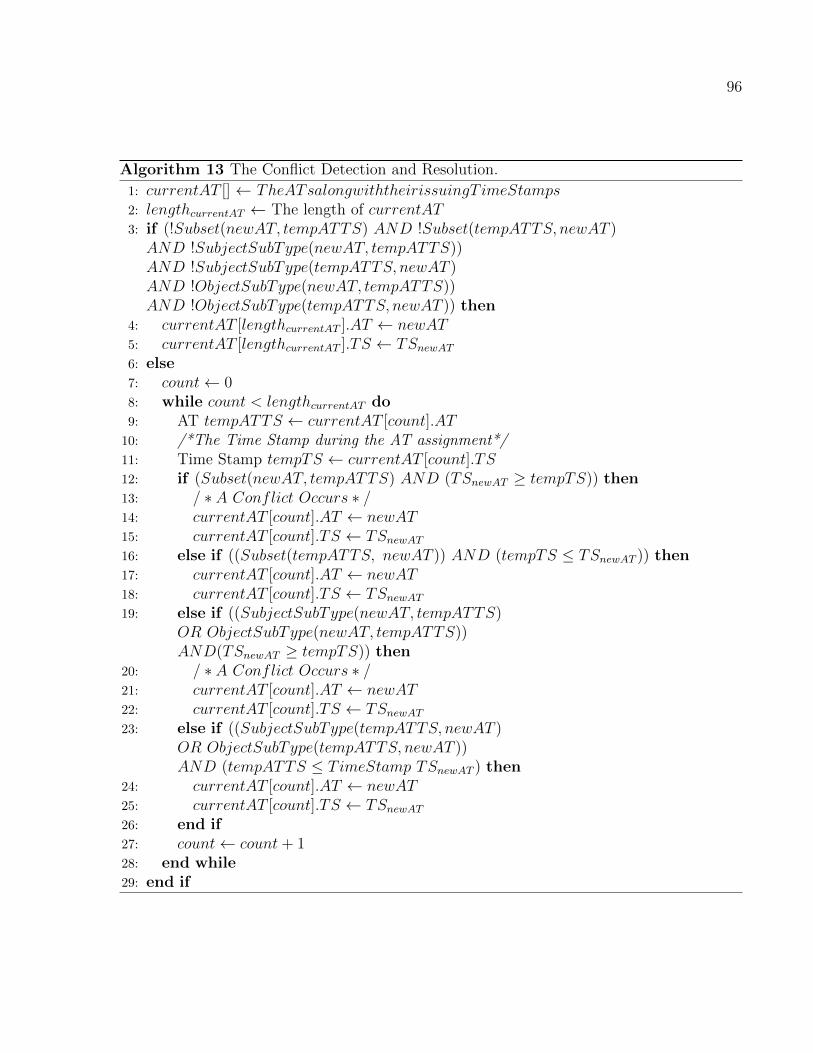
96
Algorithm 13 The Conflict Detection and Resolution.
1: currentAT [] ← TheATsalongwiththeirissuingT imeStamps2: lengthcurrentAT ← The length of currentAT3: if (!Subset(newAT, tempATTS) AND !Subset(tempATTS, newAT )AND !SubjectSubType(newAT, tempATTS))AND !SubjectSubType(tempATTS, newAT )AND !ObjectSubType(newAT, tempATTS))AND !ObjectSubType(tempATTS, newAT )) then
4: currentAT [lengthcurrentAT ].AT ← newAT5: currentAT [lengthcurrentAT ].TS ← TSnewAT6: else7: count← 08: while count < lengthcurrentAT do9: AT tempATTS ← currentAT [count].AT10: /*The Time Stamp during the AT assignment*/11: Time Stamp tempTS ← currentAT [count].TS12: if (Subset(newAT, tempATTS) AND (TSnewAT ≥ tempTS)) then13: / ∗ A Conflict Occurs ∗ /14: currentAT [count].AT ← newAT15: currentAT [count].TS ← TSnewAT16: else if ((Subset(tempATTS, newAT )) AND (tempTS ≤ TSnewAT )) then17: currentAT [count].AT ← newAT18: currentAT [count].TS ← TSnewAT19: else if ((SubjectSubType(newAT, tempATTS)
OR ObjectSubType(newAT, tempATTS))AND(TSnewAT ≥ tempTS)) then
20: / ∗ A Conflict Occurs ∗ /21: currentAT [count].AT ← newAT22: currentAT [count].TS ← TSnewAT23: else if ((SubjectSubType(tempATTS, newAT )
OR ObjectSubType(tempATTS, newAT ))AND (tempATTS ≤ TimeStamp TSnewAT ) then
24: currentAT [count].AT ← newAT25: currentAT [count].TS ← TSnewAT26: end if27: count← count+ 128: end while29: end if
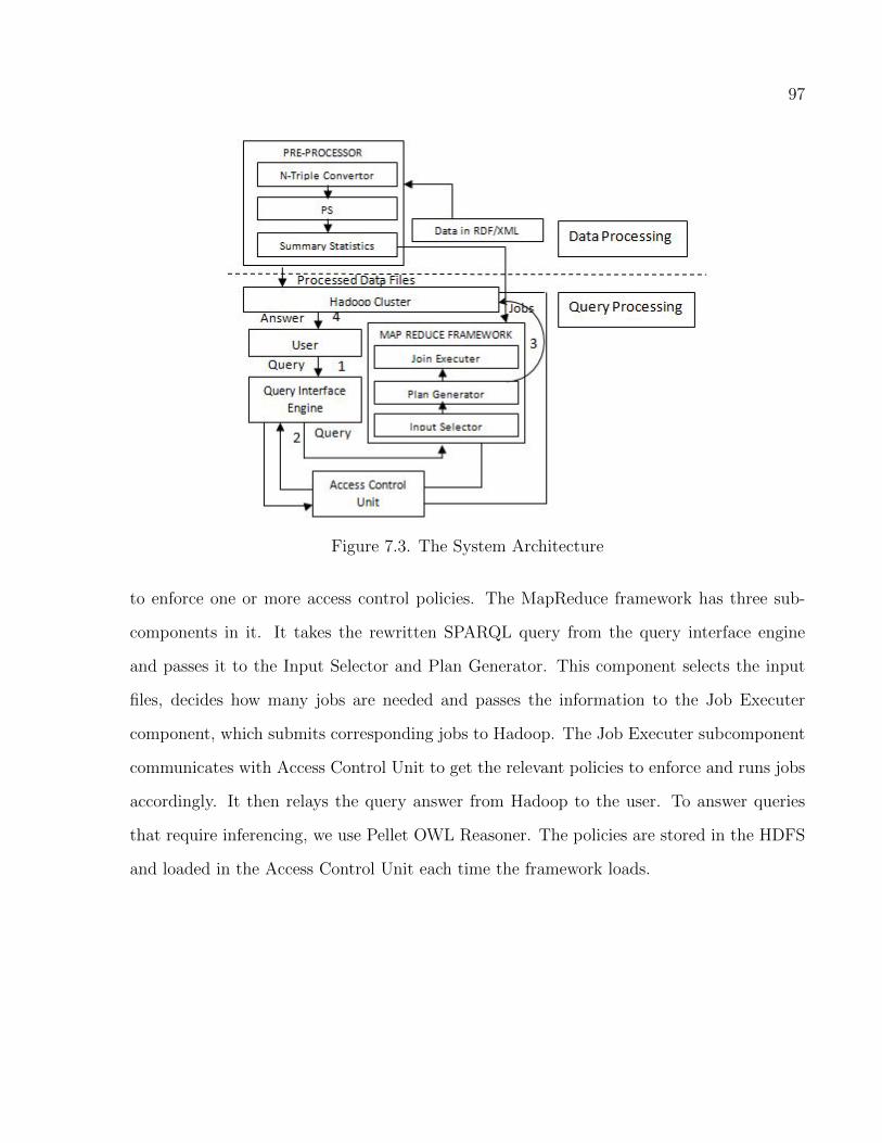
97
Figure 7.3. The System Architecture
to enforce one or more access control policies. The MapReduce framework has three sub-
components in it. It takes the rewritten SPARQL query from the query interface engine
and passes it to the Input Selector and Plan Generator. This component selects the input
files, decides how many jobs are needed and passes the information to the Job Executer
component, which submits corresponding jobs to Hadoop. The Job Executer subcomponent
communicates with Access Control Unit to get the relevant policies to enforce and runs jobs
accordingly. It then relays the query answer from Hadoop to the user. To answer queries
that require inferencing, we use Pellet OWL Reasoner. The policies are stored in the HDFS
and loaded in the Access Control Unit each time the framework loads.
98
7.3 Policy Enforcement
In our MapReduce framework we can enforce policies in two phases. We can enforce some
policies by simply rewriting a SPARQL query in query parsing phase. Rest of the policies
can be enforced in the query answering phase in two ways. First, we can enforce the policies
as we run MapReduce jobs to answer a query. Second, we can run the jobs for a query as
if there is no policy to enforce and then take the output and run a set of jobs at the end to
enforce the policies. These set of later jobs is called filter jobs. In both cases, we enforce
predicate level policies while we select the input files by the Input Selector. In the following
sections we talk about these approaches in detail.
7.3.1 Query Rewriting
Policies involving predicates can be enforced by rewriting a SPARQL query. We can replace
predicate variables by the predicates a user has permission on. An example illustrates this.
Suppose a user has a token 1, where 1 is described by 〈1 , P redicate, takesCourses, 〉 i.e.
he can only access the predicate file takesCourse. If the user submits the query listed in
Listing 7.1, we can replace the predicate variable ?p with takesCourse. The rewritten query
is shown in Listing 7.2.
Listing 7.1. Example Query
SELECT ?o WHERE{
A ?p ?o}
Listing 7.2. Rewritten Query
SELECT ?o WHERE{
A takesCourse ?o}
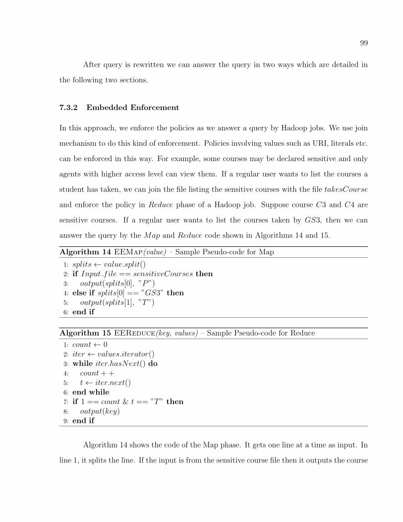
99
After query is rewritten we can answer the query in two ways which are detailed in
the following two sections.
7.3.2 Embedded Enforcement
In this approach, we enforce the policies as we answer a query by Hadoop jobs. We use join
mechanism to do this kind of enforcement. Policies involving values such as URI, literals etc.
can be enforced in this way. For example, some courses may be declared sensitive and only
agents with higher access level can view them. If a regular user wants to list the courses a
student has taken, we can join the file listing the sensitive courses with the file takesCourse
and enforce the policy in Reduce phase of a Hadoop job. Suppose course C3 and C4 are
sensitive courses. If a regular user wants to list the courses taken by GS3, then we can
answer the query by the Map and Reduce code shown in Algorithms 14 and 15.
Algorithm 14 EEMap(value) – Sample Pseudo-code for Map
1: splits← value.split()2: if Input file == sensitiveCourses then3: output(splits[0], ”P”)4: else if splits[0] == ”GS3” then5: output(splits[1], ”T”)6: end if
Algorithm 15 EEReduce(key, values) – Sample Pseudo-code for Reduce
1: count← 02: iter ← values.iterator()3: while iter.hasNext() do4: count+ +5: t← iter.next()6: end while7: if 1 == count & t == ”T” then8: output(key)9: end if
Algorithm 14 shows the code of the Map phase. It gets one line at a time as input. In
line 1, it splits the line. If the input is from the sensitive course file then it outputs the course
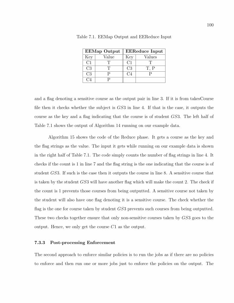
100
Table 7.1. EEMap Output and EEReduce Input
EEMap Output EEReduce InputKey Value Key ValuesC1 T C1 TC3 T C3 T, PC3 P C4 PC4 P
and a flag denoting a sensitive course as the output pair in line 3. If it is from takesCourse
file then it checks whether the subject is GS3 in line 4. If that is the case, it outputs the
course as the key and a flag indicating that the course is of student GS3. The left half of
Table 7.1 shows the output of Algorithm 14 running on our example data.
Algorithm 15 shows the code of the Reduce phase. It gets a course as the key and
the flag strings as the value. The input it gets while running on our example data is shown
in the right half of Table 7.1. The code simply counts the number of flag strings in line 4. It
checks if the count is 1 in line 7 and the flag string is the one indicating that the course is of
student GS3. If such is the case then it outputs the course in line 8. A sensitive course that
is taken by the student GS3 will have another flag which will make the count 2. The check if
the count is 1 prevents those courses from being outputted. A sensitive course not taken by
the student will also have one flag denoting it is a sensitive course. The check whether the
flag is the one for course taken by student GS3 prevents such courses from being outputted.
These two checks together ensure that only non-sensitive courses taken by GS3 goes to the
output. Hence, we only get the course C1 as the output.
7.3.3 Post-processing Enforcement
The second approach to enforce similar policies is to run the jobs as if there are no policies
to enforce and then run one or more jobs just to enforce the policies on the output. The
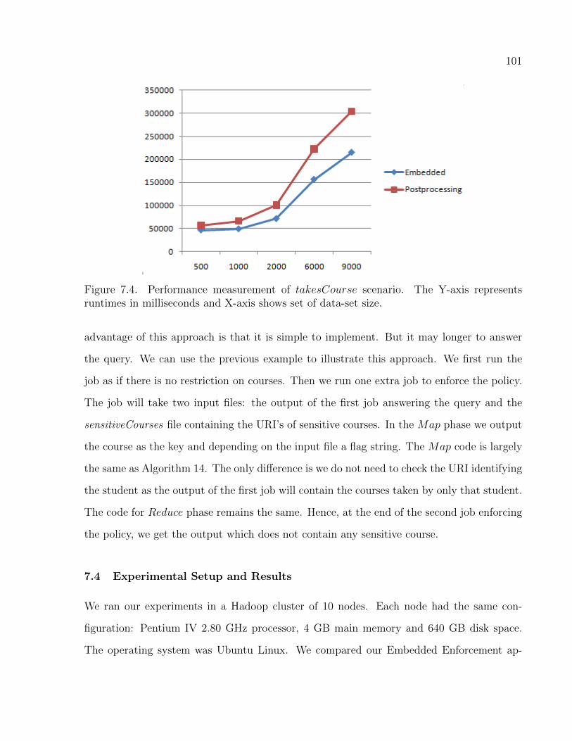
101
Figure 7.4. Performance measurement of takesCourse scenario. The Y-axis representsruntimes in milliseconds and X-axis shows set of data-set size.
advantage of this approach is that it is simple to implement. But it may longer to answer
the query. We can use the previous example to illustrate this approach. We first run the
job as if there is no restriction on courses. Then we run one extra job to enforce the policy.
The job will take two input files: the output of the first job answering the query and the
sensitiveCourses file containing the URI’s of sensitive courses. In the Map phase we output
the course as the key and depending on the input file a flag string. The Map code is largely
the same as Algorithm 14. The only difference is we do not need to check the URI identifying
the student as the output of the first job will contain the courses taken by only that student.
The code for Reduce phase remains the same. Hence, at the end of the second job enforcing
the policy, we get the output which does not contain any sensitive course.
7.4 Experimental Setup and Results
We ran our experiments in a Hadoop cluster of 10 nodes. Each node had the same con-
figuration: Pentium IV 2.80 GHz processor, 4 GB main memory and 640 GB disk space.
The operating system was Ubuntu Linux. We compared our Embedded Enforcement ap-
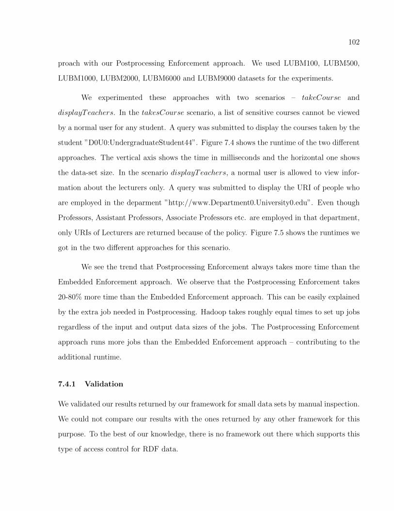
102
proach with our Postprocessing Enforcement approach. We used LUBM100, LUBM500,
LUBM1000, LUBM2000, LUBM6000 and LUBM9000 datasets for the experiments.
We experimented these approaches with two scenarios – takeCourse and
displayTeachers. In the takesCourse scenario, a list of sensitive courses cannot be viewed
by a normal user for any student. A query was submitted to display the courses taken by the
student ”D0U0:UndergraduateStudent44”. Figure 7.4 shows the runtime of the two different
approaches. The vertical axis shows the time in milliseconds and the horizontal one shows
the data-set size. In the scenario displayTeachers, a normal user is allowed to view infor-
mation about the lecturers only. A query was submitted to display the URI of people who
are employed in the deparment ”http://www.Department0.University0.edu”. Even though
Professors, Assistant Professors, Associate Professors etc. are employed in that department,
only URIs of Lecturers are returned because of the policy. Figure 7.5 shows the runtimes we
got in the two different approaches for this scenario.
We see the trend that Postprocessing Enforcement always takes more time than the
Embedded Enforcement approach. We observe that the Postprocessing Enforcement takes
20-80% more time than the Embedded Enforcement approach. This can be easily explained
by the extra job needed in Postprocessing. Hadoop takes roughly equal times to set up jobs
regardless of the input and output data sizes of the jobs. The Postprocessing Enforcement
approach runs more jobs than the Embedded Enforcement approach – contributing to the
additional runtime.
7.4.1 Validation
We validated our results returned by our framework for small data sets by manual inspection.
We could not compare our results with the ones returned by any other framework for this
purpose. To the best of our knowledge, there is no framework out there which supports this
type of access control for RDF data.
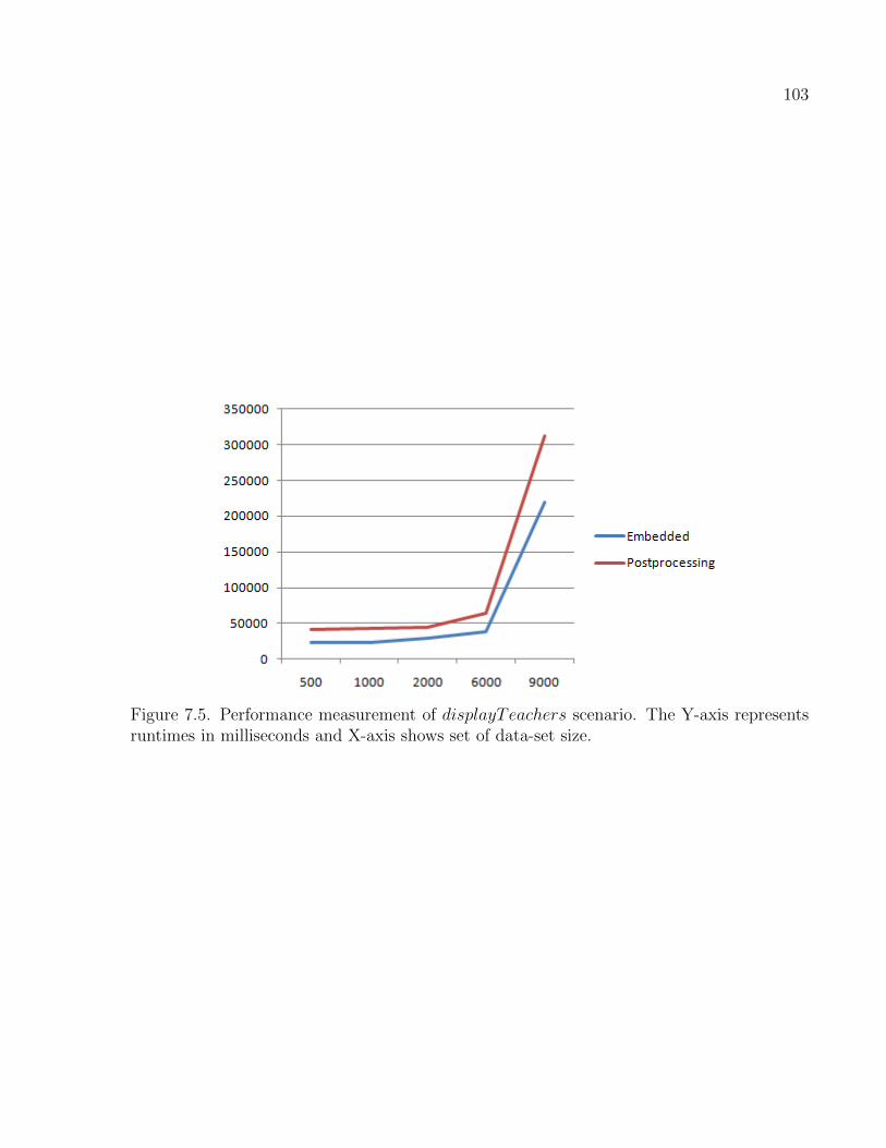
103
Figure 7.5. Performance measurement of displayTeachers scenario. The Y-axis representsruntimes in milliseconds and X-axis shows set of data-set size.
CHAPTER 8
CONCLUSION AND FUTURE WORK
8.1 Conclusion
We have presented a framework capable of handling enormous amount of RDF data. Since
our framework is based on Hadoop, which is a distributed and highly fault tolerant system,
it inherits these two properties automatically. We have successfully executed queries with
nodes deliberately turned off to test the framework’s fault tolerance. The framework is highly
scalable. To increase capacity of our system all that needs to be done is to add new nodes
to the Hadoop cluster. We use commodity class machines in our cluster.
We have proposed a schema to store RDF data. The schema allows us to select small
input data set to answer a query. This enables us to answer queries faster. Since, a file is
the smallest unit of input to a Hadoop job, the less number of files we select the faster a job
runs. Moreover, the files should be as small as possible. Our schema helps us achieve both.
We further leverage our schema by rewriting SPARQL queries. We devised an algo-
rithm which can get rid of triple patterns from a query and simplifies it in most of the cases.
A query with less number of triple patterns has requires less input data and has less number
of joins that one with more triple patterns. Hence, the query rewriting algorithm gives us
significant improvement in query running times.
We have multiple algorithms to determine a query processing plan to answer a
SPARQL query and a simplified cost model to be used by the algorithms. Since the search
space is exponential in size, we attack the problem with two approaches:
104
105
• exhaustively enumerate all the plans using graph coloring scheme and pick the best
one
• greedily find the best one using heuristics.
In practice, our exhaustive enumeration algorithm runs very quickly for real world queries.
Real world queries typically has less than hundred joins for which the query plan generation
time by the exhaustive enumeration algorithm is negligible in comparison to the actual query
answering time. However, our greedy algorithms are very fast to generate a plan for any
query. We also have extended those algorithms to generate query plan for complex SPARQL
queries having OPTIONAL query blocks.
Our experiments demonstrate that our system is highly scalable. If we increase the
data volume, the delay introduced to answer a query does not increase proportionally. The
results indicate that for very large data sets (over 1 billion triples) HadoopRDF is preferable
and more efficient if the query includes low selectivity joins or significant inference.
8.2 Limitations
While our framework has excellent scalability and is very efficient in answering queries over
large data sets, we did identify few limitations:
• Our framework splits each data set into a number of files that is proportional to the
number of unique predicates in the data set. If the number of unique predicates is
extremely large (e.g., in the millions), then this is intractable for standard file systems.
This is not a limitation in practical scenarios that we have encountered thus far because
useful, real-world data sets have records that mostly reuse a relatively small set of
predicates.
106
• In the same scenario, our exhaustive search algorithm for generating query plans would
take an impractical amount of time to generate a plan if the number of triple patterns
(see Definition 1 in Section 4.3) a query contains is very large resulting in a large
number of joins (e.g. in the hundreds or more). The running time of the algorithm is
exponential in the number of joins and so the algorithm does not scale well for such
queries. In such a scenario, we can use our heuristic based greedy algorithm for plan
generation.
8.3 Future Work
In the future, we would like to extend the work in few directions.
8.3.1 Sophisticated Query Model
We will investigate more sophisticated query model. As extensive statistics gathering is
expensive, we will mine for frequent queries (Baeza-Yates 2005; Yang, Lee, and Hsu 2003;
Yang, Lee, Hsu, and Acharya 2003). We will cache statistics for the most frequent queries
and use dynamic programming to exploit the statistics (Gilbert, Kotidis, Muthukrishnan,
and Strauss 2001; Gonul and Shi 1998).
8.3.2 Experiment with Number of Reducers
We will evaluate the impact of the number of reducers, the only parameter of a Hadoop
job specifiable by user, on the query running times. We have done some experiments with
the numbers but extensive experiments need to be done to better understand its impact.
Intuitively, the more reducer the quicker the query may run (Jenkin 2009). But very large
number of reducers may not be better if the number of reducers exceed the number of avail-
107
able TaskTracker† nodes in the cluster. In such a case, we observed that, in a TaskTracker,
the reducers are ran serially rather than in parallel. This slow downs the query running time
instead of making it quicker.
8.3.3 Indexing
We will investigate indexing opportunities and further usage of binary formats. Our dic-
tionary encoding now allows us to do indexing based on the numeric id values. We can
exploit indexing structures like B-tree (Bayer and McCreight 1972; Bayer 1997; Comer 1979;
Lehman and Yao 1981) and B+-tree (Jensen, Tie!sytye, and Tradi!sauskas 2006; Srinivasan
and Carey 1993; Abel 1984). We can further split the files based on the ranges of the numeric
values of the objects and subjects. This would allow us to select even smaller input data for
the Hadoop jobs.
8.3.4 Different Types of SPARQL Queries
We will handle more types of SPARQL queries e.g. queries having set operations, CON-
STRUCT†, ASK†, DESCRIBE† queries etc.
Set operations like union, intersect and minus can be implemented trivially in the
final stage of the query processing. We can answer each of the distinct blocks in a SPARQL
query having set operations by treating them as separate queries. As a final step, we can
apply the set operations specified in the query on the result sets of those distinct queries.
For example, Listing 8.1 shows an example query having union operation. We can treat the
BGPs { ?X rdf:type ub:Department } and { ?Y rdf:type ub:University } as separate queries
and answer them first. Then we can combine the result sets to get the final result.
†http://wiki.apache.org/hadoop/TaskTracker†http://www.w3.org/TR/rdf-sparql-query/#construct†http://www.w3.org/TR/rdf-sparql-query/#ask†http://www.w3.org/TR/rdf-sparql-query/#describe
108
Listing 8.1. Example Union Query
SELECT ?X, ?Y, ?Z WHERE {{ ?X rd f : type ub : Department }UNION{ ?Y rd f : type ub : Un ive r s i ty }}
A CONSTRUCT query, as the name suggests, constructs an RDF graph using a
graph template. The template can have both bound or unbound i.e. variable subject,
predicate and object. The variables in a triple pattern in the template have to bound to
values in matching triples in the data set. The example in Listing 8.2 taken from http:
//www.w3.org/TR/rdf-sparql-query/#construct shows a CONSTRUCT query.
Listing 8.2. Example CONSTRUCT Query
PREFIX f o a f : <http :// xmlns . com/ f o a f /0.1/>PREFIX vcard : <http ://www. w3 . org /2001/ vcard−rd f /3.0#>CONSTRUCT { <http :// example . org / person#Alice> vcard :FN ?name }WHERE { ?x f o a f : name ?name }
When the query is ran on the data shown in Listing 8.3, it returns the RDF graph
shown in Listing 8.4.
Listing 8.3. Example Data for CONSTRUCT Query
@pref ix f o a f : <http :// xmlns . com/ f o a f /0.1/> .: a f o a f : name ” Al i c e ” .: a f o a f : mbox <mai l to : a l ice@example . org> .
Listing 8.4. Resultant Graph
@pref ix vcard : <http ://www. w3 . org /2001/ vcard−rd f /3.0#> .<http :// example . org / person#Alice> vcard :FN ” Al i c e ” .
An ASK query simply checks if a query has a solution or not. It then returns a
boolean result: true if it has a solution, false otherwise. Listing 8.5 shows an example ASK
query.
Listing 8.5. Example Ask Query
ASK { ?X rd f : type ub : Un ive r s i ty }
109
We can trivially answer this query using our framework. We can first answer the
query and then check if there is a solution and return a result accordingly. We optimize this
by modifying the final job. As soon as a solution, i.e. a tuple of result is found, we can stop
processing more results and return true. Otherwise, we let the job finish and return false.
A DESCRIBE query, as the name suggests, describes the resources matched by the
variables in the query. For example Listing 8.6 shows a DESCRIBE query the result of which
would describe all the universities. An example result set is show in Listing 8.7.
Listing 8.6. Example DESCRIBE Query
DESCRIBE ?x where { ?x rd f : type ex : Un ive r s i ty }
Listing 8.7. Example Result Set for DESCRIBE Query
ex : Un ive r s i ty0 rd f : type ex : Un ive r s i tyex : Un ive r s i ty0 ex : c i t y ex : City0ex : Un ive r s i ty0 ex : country ex : County0ex : Un ive r s i ty0 ex : hasDepartment ex : ComputerScience0
We will investigate new approaches to answer DESCRIBE queries by our framework.
8.3.5 Using Hive and HBase
There are several open source frameworks for data storage and manipulation which work on
top of Hadoop. Hive† and HBase† are the most prominent ones among them.
Hive (Thusoo, Sarma, Jain, Shao, Chakka, 0002, Anthony, Liu, and Murthy 2010;
Thusoo, Sarma, Jain, Shao, Chakka, Anthony, Liu, Wyckoff, and Murthy 2009) is a data-
warehousing tool based on Hadoop which supports a SQL like language called HiveQL. It
runs MapReduce jobs to answer HiveQL† queries. It has advanced features like partitioning,
†http://hive.apache.org/†http://hbase.apache.org/†http://wiki.apache.org/hadoop/Hive/LanguageManual
110
indexing, compression etc. Hive is developed by a Facebook team and made open source. It
is widely being used as a data warehouse tool.
HBase is a column oriented store modeled after BigTable (Chang, Dean, Ghemawat,
Hsieh, Wallach, Burrows, Chandra, Fikes, and Gruber 2006). It has features like indexing,
bloom filters etc. It supports querying through APIs and runs MapReduce jobs to answer
queries based on the type of query. HBase is also being used by big enterprizes. We will
investigate various schemas with these tools and experiment with their features to achieve
fast query running times.
8.3.6 Inferencing
We will add support for inferencing in our framework. We can use libraries for OWL DL
inferencing like Pellet (Sirin, Parsia, Grau, Kalyanpur, and Katz 2007), FaCT++ (Tsarkov
and Horrocks 2006) for this purpose. We will add forward chaining to the framework so that
we can infer new triples at loading time. There has been some work on forward chaining using
MapReduce and other parallel programming approaches (Urbani, Kotoulas, Oren, and van
Harmelen 2009; Urbani 2010; Soma and Prasanna 2008; Oren, Kotoulas, Anadiotis, Siebes,
ten Teije, and van Harmelen 2009; Schlicht and Stuckenschmidt 2008) which we would like
to extend and apply to our framework.
REFERENCES
Abadi, D. J. (2009). Data management in the cloud: Limitations and opportunities. IEEE
Data Eng. Bull. 32 (1), 3–12.
Abadi, D. J., A. Marcus, S. Madden, and K. Hollenbach (2009). Sw-store: a vertically
partitioned dbms for semantic web data management. VLDB J. 18 (2), 385–406.
Abadi, D. J., A. Marcus, S. Madden, and K. J. Hollenbach (2007). Scalable semantic web
data management using vertical partitioning. In VLDB, pp. 411–422.
Abel, D. J. (1984). A b+-tree structure for large quadtrees. Computer Vision, Graphics,
and Image Processing 27 (1), 19–31.
Abouzeid, A., K. Bajda-Pawlikowski, D. J. Abadi, A. Rasin, and A. Silberschatz (2009).
Hadoopdb: An architectural hybrid of mapreduce and dbms technologies for analytical
workloads. PVLDB 2 (1), 922–933.
Atre, M., J. Srinivasan, and J. A. Hendler (2008). Bitmat: A main-memory bit matrix
of rdf triples for conjunctive triple pattern queries. In International Semantic Web
Conference (Posters & Demos).
Baeza-Yates, R. A. (2005). Applications of web query mining. In ECIR, pp. 7–22.
Bayer, R. (1997). The universal b-tree for multidimensional indexing: general concepts.
In WWCA, pp. 198–209.
Bayer, R. and E. M. McCreight (1972). Organization and maintenance of large ordered
indices. Acta Inf. 1, 173–189.
Bayir, M. A., I. H. Toroslu, A. Cosar, and G. Fidan (2009). Smart miner: a new framework
for mining large scale web usage data. In WWW, pp. 161–170.
Boncz, P. A., T. Grust, M. van Keulen, S. Manegold, J. Rittinger, and J. Teubner (2006).
Monetdb/xquery: a fast xquery processor powered by a relational engine. In SIGMOD
Conference, pp. 479–490.
Bose, J.-H., A. Andrzejak, and M. Hogqvist (2010). Beyond online aggregation: paral-
lel and incremental data mining with online map-reduce. In Proceedings of the 2010
Workshop on Massive Data Analytics on the Cloud, MDAC ’10, New York, NY, USA,
pp. 3:1–3:6. ACM.
Bouganim, L., F. D. Ngoc, and P. Pucheral (2004). Client-based access control manage-
ment for xml documents. In BDA, pp. 65–89.
111
112
Broekstra, J., A. Kampman, and F. van Harmelen (2002). Sesame: A generic architecture
for storing and querying rdf and rdf schema. In International Semantic Web Confer-
ence, pp. 54–68.
Bu, Y., B. Howe, M. Balazinska, and M. Ernst (2010). Haloop: Efficient iterative data
processing on large clusters. PVLDB 3 (1), 285–296.
Carroll, J. J., I. Dickinson, C. Dollin, D. Reynolds, A. Seaborne, and K. Wilkinson (2004).
Jena: implementing the semantic web recommendations. In Proceedings of the 13th
international World Wide Web conference on Alternate track papers & posters, WWW
Alt. ’04, New York, NY, USA, pp. 74–83. ACM.
Chang, E. Y., H. Bai, and K. Zhu (2009). Parallel algorithms for mining large-scale rich-
media data. In ACM Multimedia, pp. 917–918.
Chang, F., J. Dean, S. Ghemawat, W. C. Hsieh, D. A. Wallach, M. Burrows, T. Chandra,
A. Fikes, and R. Gruber (2006). Bigtable: A distributed storage system for structured
data (awarded best paper!). In OSDI, pp. 205–218.
Chebotko, A., S. Lu, and F. Fotouhi (2009, October). Semantics preserving sparql-to-sql
translation. Data Knowl. Eng. 68, 973–1000.
Chong, E. I., S. Das, G. Eadon, and J. Srinivasan (2005). An efficient sql-based rdf querying
scheme. In Proceedings of the 31st international conference on Very large data bases,
VLDB ’05, pp. 1216–1227. VLDB Endowment.
Chu, C. T., S. K. Kim, Y. A. Lin, Y. Yu, G. R. Bradski, A. Y. Ng, and K. Olukotun
(2006). Map-reduce for machine learning on multicore. In B. Scholkopf, J. C. Platt,
and T. Hoffman (Eds.), NIPS, pp. 281–288. MIT Press.
Comer, D. (1979, June). Ubiquitous b-tree. ACM Comput. Surv. 11, 121–137.
Cook, S. A. (1971). The complexity of theorem-proving procedures. In Proceedings of the
third annual ACM symposium on Theory of computing, STOC ’71, New York, NY,
USA, pp. 151–158. ACM.
Cyganiak, R. (2005). A relational algebra for sparql. Digital Media Systems Laboratory
HP Laboratories Bristol. HPL-2005-170 .
Das, S., Y. Sismanis, K. S. Beyer, R. Gemulla, P. J. Haas, and J. McPherson (2010).
Ricardo: integrating r and hadoop. In Proceedings of the 2010 international conference
on Management of data, SIGMOD ’10, New York, NY, USA, pp. 987–998. ACM.
Dean, J. and S. Ghemawat (2008, January). Mapreduce: simplified data processing on
large clusters. Commun. ACM 51, 107–113.
Ding, L., T. Finin, Y. Peng, P. P. da Silva, and D. L. Mcguinness (2005). Tracking rdf
graph provenance using rdf molecules.
113
Farhan Husain, M., P. Doshi, L. Khan, and B. Thuraisingham (2009). Storage and re-
trieval of large rdf graph using hadoop and mapreduce. In Proceedings of the 1st In-
ternational Conference on Cloud Computing, CloudCom ’09, Berlin, Heidelberg, pp.
680–686. Springer-Verlag.
Fredman, M. L. and R. E. Tarjan (1987, July). Fibonacci heaps and their uses in improved
network optimization algorithms. J. ACM 34, 596–615.
Gilbert, A. C., Y. Kotidis, S. Muthukrishnan, and M. J. Strauss (2001). Optimal and
approximate computation of summary statistics for range aggregates. In Proceedings of
the twentieth ACM SIGMOD-SIGACT-SIGART symposium on Principles of database
systems, PODS ’01, New York, NY, USA, pp. 227–236. ACM.
Gonul, F. and M. Shi (1998). Optimal mailing of catalogs: A new methodology using
estimable structural dynamic programming models. Management Science, 1249–1262.
Grossman, R. and Y. Gu (2008). Data mining using high performance data clouds: ex-
perimental studies using sector and sphere. In Proceeding of the 14th ACM SIGKDD
international conference on Knowledge discovery and data mining, KDD ’08, New
York, NY, USA, pp. 920–927. ACM.
Guo, Y., Z. Pan, and J. Heflin (2004). An evaluation of knowledge base systems for large
owl datasets. The Semantic Web–ISWC 2004 , 274–288.
Guo, Y., Z. Pan, and J. Heflin (2005, October). Lubm: A benchmark for owl knowledge
base systems. Web Semant. 3, 158–182.
Heinz, S., J. Zobel, and H. E. Williams (2002, April). Burst tries: a fast, efficient data
structure for string keys. ACM Trans. Inf. Syst. 20, 192–223.
Holmquist, L., J. Redstrom, and P. Ljungstrand (1999). Token-based access to digital
information. In Handheld and Ubiquitous Computing, pp. 234–245. Springer.
Jain, A. and C. Farkas (2006). Secure resource description framework: an access control
model. In Proceedings of the eleventh ACM symposium on Access control models and
technologies, SACMAT ’06, New York, NY, USA, pp. 121–129. ACM.
Jenkin, N. (2009). Distributed machine learning with hadoop. Technical Report
COMP390-09A Report.
Jensen, C. S., D. Tie!sytye, and N. Tradi!sauskas (2006). Robust b+-tree-based indexing
of moving objects. In Proceedings of the 7th International Conference on Mobile Data
Management, MDM ’06, Washington, DC, USA, pp. 12–. IEEE Computer Society.
Kiryakov, A., D. Ognyanov, and D. Manov (2005). Owlim a pragmatic semantic repository
for owl. pp. 182–192.
Lehman, P. L. and s. B. Yao (1981, December). Efficient locking for concurrent operations
on b-trees. ACM Trans. Database Syst. 6, 650–670.
114
McBride, B. (2002, November). Jena: A semantic web toolkit. IEEE Internet Comput-
ing 6, 55–59.
McGlothlin, J. and L. Khan (2010a). A semantic web repository for managing and querying
aligned knowledge.
McGlothlin, J. P. (2010). Framework and schema for semantic web knowledge bases. In
AAAI.
McGlothlin, J. P. and L. Khan (2010b). Efficient rdf data management including prove-
nance and uncertainty. In IDEAS, pp. 193–198.
McGlothlin, J. P. and L. R. Khan (2009). Rdfkb: efficient support for rdf inference queries
and knowledge management. In IDEAS, pp. 259–266.
McGlothlin, J. P. and L. R. Khan (2010c). Materializing and persisting inferred and
uncertain knowledge in rdf datasets. In AAAI.
McNabb, A. W., C. K. Monson, and K. D. Seppi (2007). Mrpso: Mapreduce particle swarm
optimization. In Proceedings of the 9th annual conference on Genetic and evolutionary
computation, GECCO ’07, New York, NY, USA, pp. 177–177. ACM.
Mika, P. and G. Tummarello (2008, September). Web semantics in the clouds. IEEE
Intelligent Systems 23, 82–87.
Moreira, J. E., M. M. Michael, D. Da Silva, D. Shiloach, P. Dube, and L. Zhang (2007).
Scalability of the nutch search engine. In Proceedings of the 21st annual international
conference on Supercomputing, ICS ’07, New York, NY, USA, pp. 3–12. ACM.
Moretti, C., K. Steinhaeuser, D. Thain, and N. V. Chawla (2008). Scaling up classifiers
to cloud computers. In Proceedings of the 2008 Eighth IEEE International Conference
on Data Mining, Washington, DC, USA, pp. 472–481. IEEE Computer Society.
Navathe, S. and R. elmasri (2002). Fundamentals of Database Systems. Addison-Wesley.
Neumann, T. and G. Weikum (2008, August). Rdf-3x: a risc-style engine for rdf. Proc.
VLDB Endow. 1, 647–659.
Newman, A., J. Hunter, Y. F. Li, C. Bouton, and M. Davis (2008). A scale-out rdf molecule
store for distributed processing of biomedical data. In Semantic Web for Health Care
and Life Sciences Workshop (HCLS’08) at the 17th International Conference on World
Wide Web (WWW’08).
Olston, C., B. Reed, U. Srivastava, R. Kumar, and A. Tomkins (2008). Pig latin: a not-
so-foreign language for data processing. In Proceedings of the 2008 ACM SIGMOD
international conference on Management of data, SIGMOD ’08, New York, NY, USA,
pp. 1099–1110. ACM.
115
Oren, E., S. Kotoulas, G. Anadiotis, R. Siebes, A. ten Teije, and F. van Harmelen (2009).
Marvin: Distributed reasoning over large-scale semantic web data. J. Web Sem. 7 (4),
305–316.
Papadimitriou, S. and J. Sun (2008). Disco: Distributed co-clustering with map-reduce:
A case study towards petabyte-scale end-to-end mining. In Proceedings of the 2008
Eighth IEEE International Conference on Data Mining, Washington, DC, USA, pp.
512–521. IEEE Computer Society.
Reddivari, P., T. Finin, and A. Joshi (2005, May). Policy based access control for a rdf
store. In Proceedings of the Policy Management for the Web Workshop, A WWW 2005
Workshop.
Rohloff, K., M. Dean, I. Emmons, D. Ryder, and J. Sumner (2007). An evaluation of triple-
store technologies for large data stores. In Proceedings of the 2007 OTM Confederated
international conference on On the move to meaningful internet systems - Volume Part
II, OTM’07, Berlin, Heidelberg, pp. 1105–1114. Springer-Verlag.
Rosenthal, A. and U. S. Chakravarthy (1988). Anatomy of a mudular multiple query
optimizer. In VLDB, pp. 230–239.
Schlicht, A. and H. Stuckenschmidt (2008). Distributed resolution for alc. In Description
Logics.
Schmidt, M., T. Hornung, G. Lausen, and C. Pinkel (2008). Sp2bench: A sparql perfor-
mance benchmark. CoRR abs/0806.4627.
Sidirourgos, L., R. Goncalves, M. Kersten, N. Nes, and S. Manegold (2008, August).
Column-store support for rdf data management: not all swans are white. Proc. VLDB
Endow. 1, 1553–1563.
Sirin, E., B. Parsia, B. C. Grau, A. Kalyanpur, and Y. Katz (2007, June). Pellet: A
practical owl-dl reasoner. Web Semant. 5, 51–53.
Soma, R. and V. K. Prasanna (2008). Parallel inferencing for owl knowledge bases. In
Proceedings of the 2008 37th International Conference on Parallel Processing, ICPP
’08, Washington, DC, USA, pp. 75–82. IEEE Computer Society.
Srinivasan, V. and M. J. Carey (1993, October). Performance of b+ tree concurrency
control algorithms. The VLDB Journal 2, 361–406.
Stocker, M., A. Seaborne, A. Bernstein, C. Kiefer, and D. Reynolds (2008). Sparql ba-
sic graph pattern optimization using selectivity estimation. In Proceeding of the 17th
international conference on World Wide Web, WWW ’08, New York, NY, USA, pp.
595–604. ACM.
Stonebraker, M., D. J. Abadi, A. Batkin, X. Chen, M. Cherniack, M. Ferreira, E. Lau,
A. Lin, S. Madden, E. O’Neil, P. O’Neil, A. Rasin, N. Tran, and S. Zdonik (2005).
116
C-store: a column-oriented dbms. In Proceedings of the 31st international conference
on Very large data bases, VLDB ’05, pp. 553–564. VLDB Endowment.
Thusoo, A., J. S. Sarma, N. Jain, Z. Shao, P. Chakka, N. Z. 0002, S. Anthony, H. Liu, and
R. Murthy (2010). Hive - a petabyte scale data warehouse using hadoop. In ICDE, pp.
996–1005.
Thusoo, A., J. S. Sarma, N. Jain, Z. Shao, P. Chakka, S. Anthony, H. Liu, P. Wyckoff,
and R. Murthy (2009). Hive - a warehousing solution over a map-reduce framework.
PVLDB 2 (2), 1626–1629.
Tsarkov, D. and I. Horrocks (2006). Fact++ description logic reasoner: System descrip-
tion. In Proc. of the Int. Joint Conf. on Automated Reasoning (IJCAR 2006), Volume
4130 of Lecture Notes in Artificial Intelligence, pp. 292–297. Springer.
Ullman, J. (1980). Principles of database systems. Computer Science Press Maryland,
USA.
Ullmann, J. R. (1976, January). An algorithm for subgraph isomorphism. J. ACM 23,
31–42.
Urbani, J. (2010). Scalable and parallel reasoning in the semantic web. In ESWC (2), pp.
488–492.
Urbani, J., S. Kotoulas, E. Oren, and F. van Harmelen (2009). Scalable distributed rea-
soning using mapreduce. In International Semantic Web Conference, pp. 634–649.
Wang, J., S. Wu, H. Gao, J. Li, and B. C. Ooi (2010). Indexing multi-dimensional data
in a cloud system. In Proceedings of the 2010 international conference on Management
of data, SIGMOD ’10, New York, NY, USA, pp. 591–602. ACM.
Weiss, C., P. Karras, and A. Bernstein (2008, August). Hexastore: sextuple indexing for
semantic web data management. Proc. VLDB Endow. 1, 1008–1019.
Xu, Y., P. Kostamaa, and L. Gao (2010). Integrating hadoop and parallel dbms. In Pro-
ceedings of the 2010 international conference on Management of data, SIGMOD ’10,
New York, NY, USA, pp. 969–974. ACM.
Yan, R., M.-O. Fleury, M. Merler, A. Natsev, and J. R. Smith (2009). Large-scale mul-
timedia semantic concept modeling using robust subspace bagging and mapreduce.
In Proceedings of the First ACM workshop on Large-scale multimedia retrieval and
mining, LS-MMRM ’09, New York, NY, USA, pp. 35–42. ACM.
Yang, L. H., M. L. Lee, and W. Hsu (2003). Efficient mining of xml query patterns for
caching. In Proceedings of the 29th international conference on Very large data bases -
Volume 29, VLDB ’2003, pp. 69–80. VLDB Endowment.

117
Yang, L. H., M. L. Lee, W. Hsu, and S. Acharya (2003). Mining frequent quer patterns
from xml queries. In Proceedings of the Eighth International Conference on Database
Systems for Advanced Applications, DASFAA ’03, Washington, DC, USA, pp. 355–.
IEEE Computer Society.
Zhao, W., H. Ma, and Q. He (2009). Parallel k-means clustering based on mapreduce. In
Proceedings of the 1st International Conference on Cloud Computing, CloudCom ’09,
Berlin, Heidelberg, pp. 674–679. Springer-Verlag.
Zobel, J., S. Heinz, and H. E. Williams (2001, December). In-memory hash tables for
accumulating text vocabularies. Inf. Process. Lett. 80, 271–277.

VITA
Mohammad Farhan Husain graduated from Bangladesh University of Engineering and Tech-
nology with a degree of BSc. Engg. in Computer Science and Engineering in August, 2004.
After that he worked as a Software Engineer in Eyeball Networks Inc. and Grameen Software
Ltd. In Fall 2006 he joined the Department of Computer Science at the University of Texas
at Dallas as a PhD student under Dr. Bhavani Thuraisingham and Dr. Latifur Khan in the
Intelligent Systems track. He interned in Sabre Holdings and Cisco Systems during the his
studentship at the university. He developed a Police Blotter tool for Raytheon which was
demonstrated in GeoInt 2009 conference in San Antonio, TX. He proposed and developed a
scalable and efficient repository and retrieval system for very large Semantic Web data. His
research has been supported in part by the AFOSR under Award No. FA9550-08-1-0260 and
Raytheon. He is going to join Amazon.com as a Software Engineer after finishing his Ph.D.