WINSASW VERSION 2.0

USER’S GUIDE

Data Interpretation and Analysis FOR SASW MEASUREMENTS

AUG. 9, 2002

DEPT. OF CIVIL ENGINEERING CHUNG-ANG UNIVERSITY, ANSEONG, KOREA

Contents

1. Installation 3 2. Overview 5 2.1 Data Interpretation and Analysis 5 2.2 Description on Main Menu 5 3. Load Measurement Data 8 3.1 ASCII Format Data 8 3.2 Experimental Dispersion Data from WinSASW 1.0 9 4. Interactive Masking 12 5. Determination of Phase Velocity Dispersion Curve 16 6. Inversion Analysis 20 6.1 Subsurface Layering and Dispersion Data for Inversion Analysis 20 6.2 Determination of the Starting Model for Inversion Analysis 23 7. Forward Modeling 28 7.1 Soil Profile and Dispersion Curves for Forward Modeling 28 7.2 Representative Experimental Dispersion Data 29 Reference 33

2

1. Installation

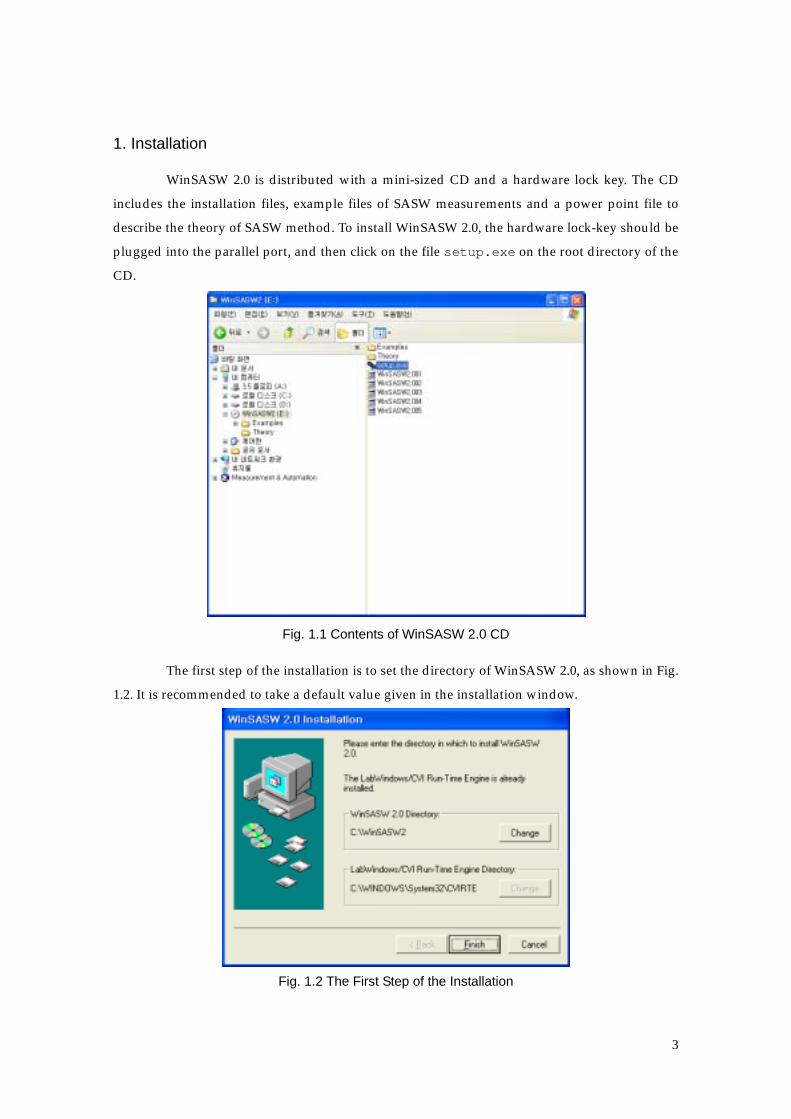
WinSASW 2.0 is distributed with a mini-sized CD and a hardware lock key. The CD

includes the installation files, example files of SASW measurements and a power point file to

describe the theory of SASW method. To install WinSASW 2.0, the hardware lock-key should be

plugged into the parallel port, and then click on the file setup.exe on the root directory of the

CD.

Fig. 1.1 Contents of WinSASW 2.0 CD

The first step of the installation is to set the directory of WinSASW 2.0, as shown in Fig.

1.2. It is recommended to take a default value given in the installation window.

Fig. 1.2 The First Step of the Installation

3

When the installation of WinSASW 2.0 is finished, the system driver of the hardware

lock key is installed. The installation of the system driver is guided by the installation wizard as

shown in Fig. 1.3.

Fig. 1.3 The Installation Wizard of the System Driver for the Hardware Lock Key

WinSASW 2.0 checks the hardware lock key in running intermittently. The incomplete

installation of the hardware lock-key system driver results in the halt of the WinSASW 2.0. It

would be very important to plug in the hardware lock key and to install its system driver

properly.

When all the installation procedure is completed, program in the start button shows

the item of WinSASW 2.0. Now it is ready to run WinSASW 2.0.

4

2. Overview

2.1 Data Interpretation and Analysis

SASW testing has an objective to evaluate the shear-wave velocity profile of subsurface. In the field, the measurements acquire the site-specific phase spectra, which indicate the phase difference between two receivers for a series of steady-state stress wave with different frequencies.

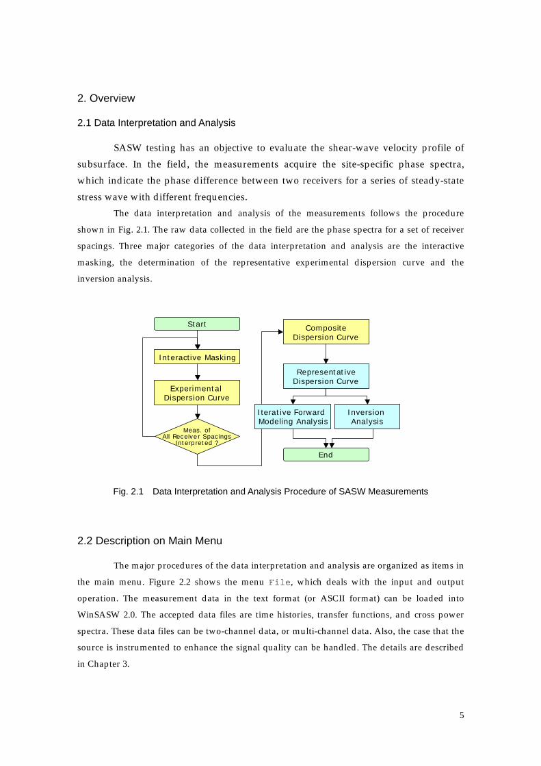
The data interpretation and analysis of the measurements follows the procedure

shown in Fig. 2.1. The raw data collected in the field are the phase spectra for a set of receiver

spacings. Three major categories of the data interpretation and analysis are the interactive

masking, the determination of the representative experimental dispersion curve and the

inversion analysis.

Start

Interactive Masking

Experimental Dispersion Curve

Meas. ofAll Receiver Spacings

Interpreted ?

CompositeDispersion Curve

RepresentativeDispersion Curve

Iterative Forward Modeling Analysis

Inversion Analysis

End

Fig. 2.1 Data Interpretation and Analysis Procedure of SASW Measurements

2.2 Description on Main Menu

The major procedures of the data interpretation and analysis are organized as items in

the main menu. Figure 2.2 shows the menu File, which deals with the input and output

operation. The measurement data in the text format (or ASCII format) can be loaded into

WinSASW 2.0. The accepted data files are time histories, transfer functions, and cross power

spectra. These data files can be two-channel data, or multi-channel data. Also, the case that the

source is instrumented to enhance the signal quality can be handled. The details are described

in Chapter 3.

5

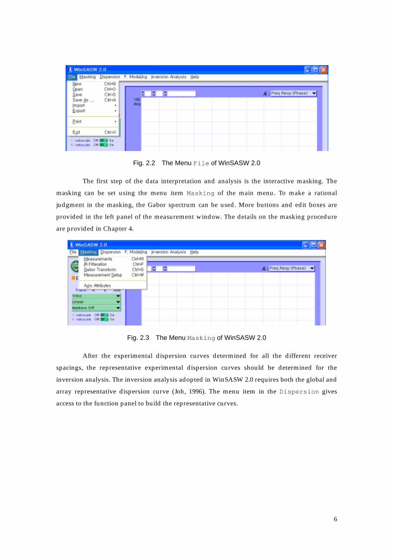
Fig. 2.2 The Menu File of WinSASW 2.0

The first step of the data interpretation and analysis is the interactive masking. The

masking can be set using the menu item Masking of the main menu. To make a rational

judgment in the masking, the Gabor spectrum can be used. More buttons and edit boxes are

provided in the left panel of the measurement window. The details on the masking procedure

are provided in Chapter 4.

Fig. 2.3 The Menu Masking of WinSASW 2.0

After the experimental dispersion curves determined for all the different receiver

spacings, the representative experimental dispersion curves should be determined for the

inversion analysis. The inversion analysis adopted in WinSASW 2.0 requires both the global and

array representative dispersion curve (Joh, 1996). The menu item in the Dispersion gives

access to the function panel to build the representative curves.

6

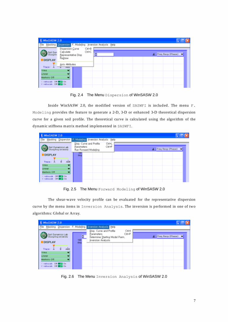
Fig. 2.4 The Menu Dispersion of WinSASW 2.0

Inside WinSASW 2.0, the modified version of SASWFI is included. The menu F.

Modeling provides the feature to generate a 2-D, 3-D or enhanced 3-D theoretical dispersion

curve for a given soil profile. The theoretical curve is calculated using the algorithm of the

dynamic stiffness matrix method implemented in SASWFI.

Fig. 2.5 The Menu Forward Modeling of WinSASW 2.0

The shear-wave velocity profile can be evaluated for the representative dispersion

curve by the menu items in Inversion Analysis. The inversion is performed in one of two

algorithms: Global or Array.

Fig. 2.6 The Menu Inversion Analysis of WinSASW 2.0

7

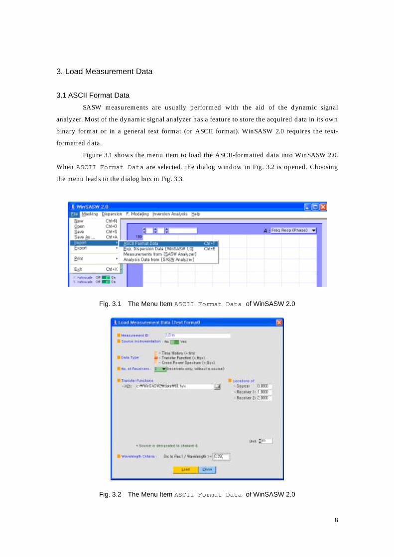
3. Load Measurement Data 3.1 ASCII Format Data SASW measurements are usually performed with the aid of the dynamic signal

analyzer. Most of the dynamic signal analyzer has a feature to store the acquired data in its own

binary format or in a general text format (or ASCII format). WinSASW 2.0 requires the text-

formatted data.

Figure 3.1 shows the menu item to load the ASCII-formatted data into WinSASW 2.0.

When ASCII Format Data are selected, the dialog window in Fig. 3.2 is opened. Choosing

the menu leads to the dialog box in Fig. 3.3.

Fig. 3.1 The Menu Item ASCII Format Data of WinSASW 2.0

Fig. 3.2 The Menu Item ASCII Format Data of WinSASW 2.0

8

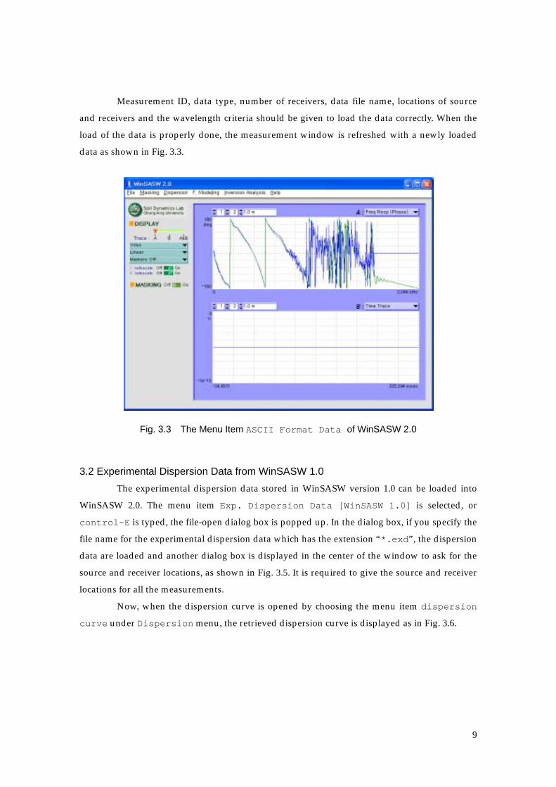
Measurement ID, data type, number of receivers, data file name, locations of source

and receivers and the wavelength criteria should be given to load the data correctly. When the

load of the data is properly done, the measurement window is refreshed with a newly loaded

data as shown in Fig. 3.3.

Fig. 3.3 The Menu Item ASCII Format Data of WinSASW 2.0

3.2 Experimental Dispersion Data from WinSASW 1.0 The experimental dispersion data stored in WinSASW version 1.0 can be loaded into

WinSASW 2.0. The menu item Exp. Dispersion Data [WinSASW 1.0] is selected, or

control-E is typed, the file-open dialog box is popped up. In the dialog box, if you specify the

file name for the experimental dispersion data which has the extension “*.exd”, the dispersion

data are loaded and another dialog box is displayed in the center of the window to ask for the

source and receiver locations, as shown in Fig. 3.5. It is required to give the source and receiver

locations for all the measurements.

Now, when the dispersion curve is opened by choosing the menu item dispersion

curve under Dispersion menu, the retrieved dispersion curve is displayed as in Fig. 3.6.

9

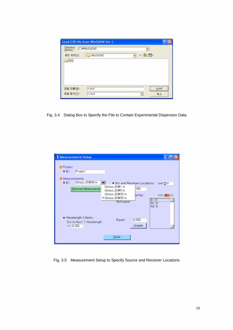
Fig. 3.4 Dialog Box to Specify the File to Contain Experimental Dispersion Data

Fig. 3.5 Measurement Setup to Specify Source and Receiver Locations

10

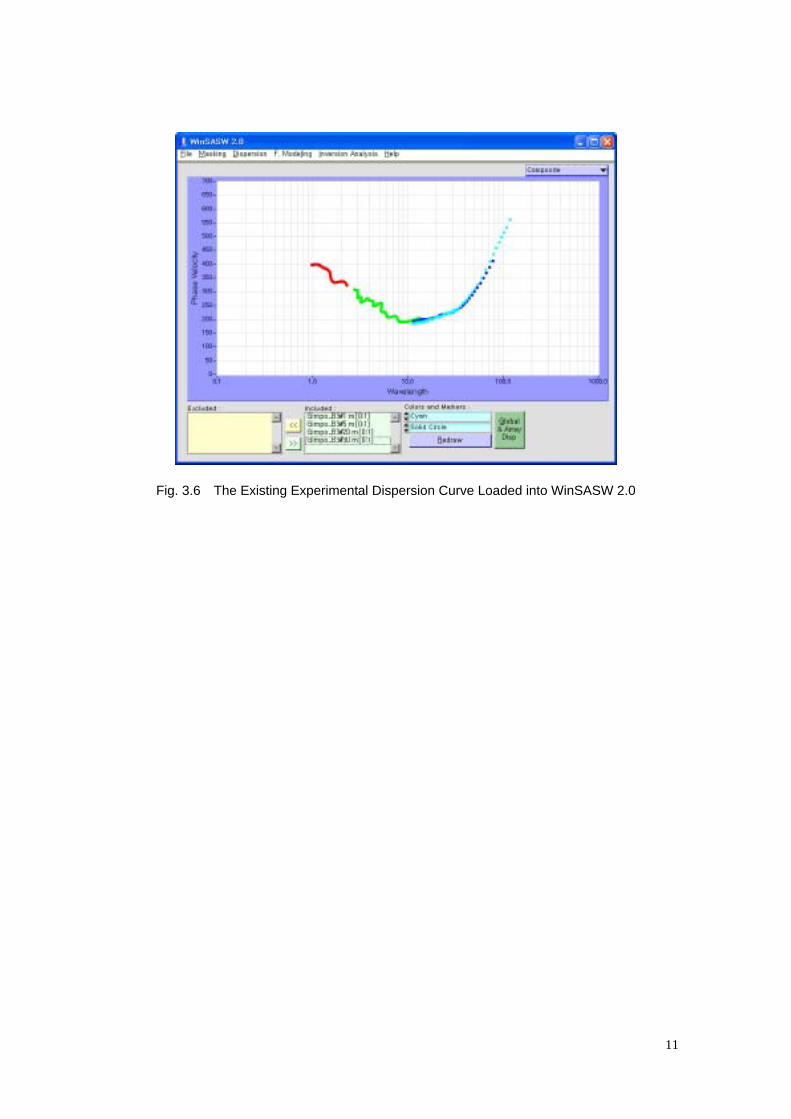
Fig. 3.6 The Existing Experimental Dispersion Curve Loaded into WinSASW 2.0

11

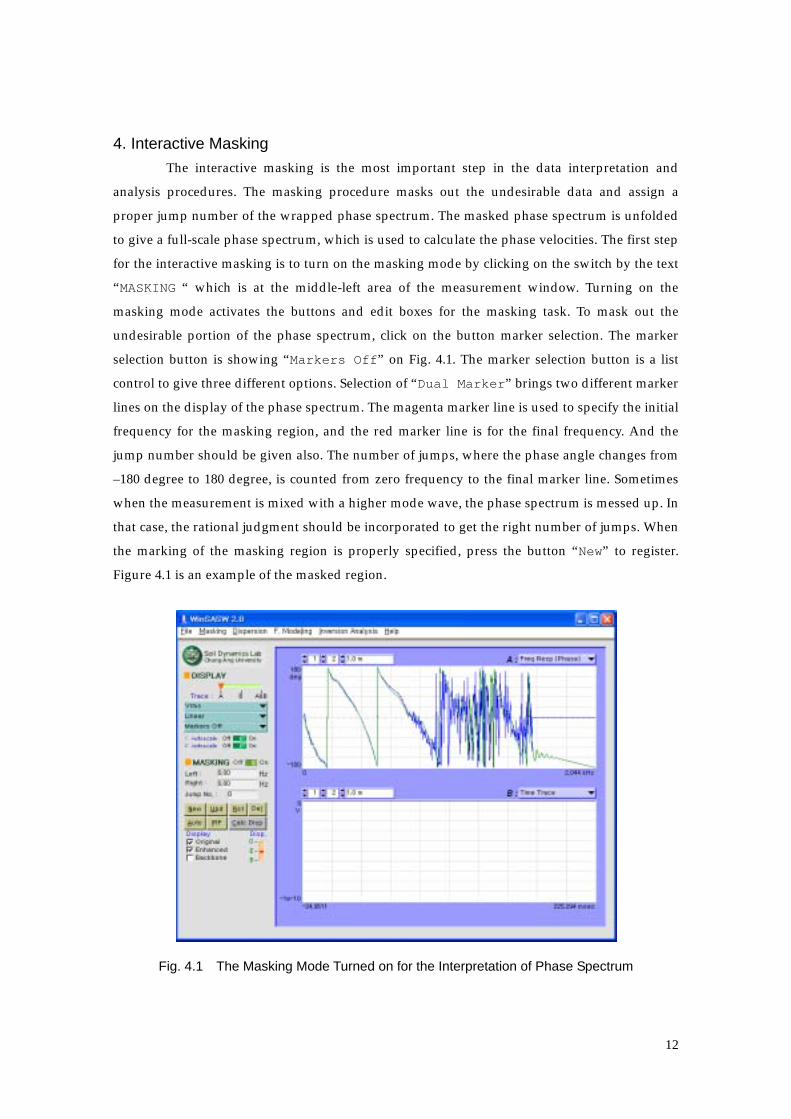
4. Interactive Masking The interactive masking is the most important step in the data interpretation and

analysis procedures. The masking procedure masks out the undesirable data and assign a

proper jump number of the wrapped phase spectrum. The masked phase spectrum is unfolded

to give a full-scale phase spectrum, which is used to calculate the phase velocities. The first step

for the interactive masking is to turn on the masking mode by clicking on the switch by the text

“MASKING “ which is at the middle-left area of the measurement window. Turning on the

masking mode activates the buttons and edit boxes for the masking task. To mask out the

undesirable portion of the phase spectrum, click on the button marker selection. The marker

selection button is showing “Markers Off” on Fig. 4.1. The marker selection button is a list

control to give three different options. Selection of “Dual Marker” brings two different marker

lines on the display of the phase spectrum. The magenta marker line is used to specify the initial

frequency for the masking region, and the red marker line is for the final frequency. And the

jump number should be given also. The number of jumps, where the phase angle changes from

–180 degree to 180 degree, is counted from zero frequency to the final marker line. Sometimes

when the measurement is mixed with a higher mode wave, the phase spectrum is messed up. In

that case, the rational judgment should be incorporated to get the right number of jumps. When

the marking of the masking region is properly specified, press the button “New” to register.

Figure 4.1 is an example of the masked region.

Fig. 4.1 The Masking Mode Turned on for the Interpretation of Phase Spectrum

12

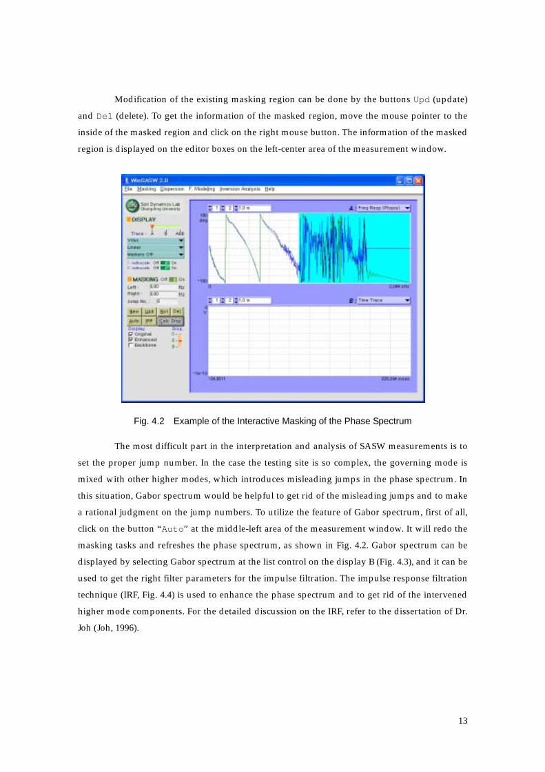
Modification of the existing masking region can be done by the buttons Upd (update)

and Del (delete). To get the information of the masked region, move the mouse pointer to the

inside of the masked region and click on the right mouse button. The information of the masked

region is displayed on the editor boxes on the left-center area of the measurement window.

Fig. 4.2 Example of the Interactive Masking of the Phase Spectrum

The most difficult part in the interpretation and analysis of SASW measurements is to

set the proper jump number. In the case the testing site is so complex, the governing mode is

mixed with other higher modes, which introduces misleading jumps in the phase spectrum. In

this situation, Gabor spectrum would be helpful to get rid of the misleading jumps and to make

a rational judgment on the jump numbers. To utilize the feature of Gabor spectrum, first of all,

click on the button “Auto” at the middle-left area of the measurement window. It will redo the

masking tasks and refreshes the phase spectrum, as shown in Fig. 4.2. Gabor spectrum can be

displayed by selecting Gabor spectrum at the list control on the display B (Fig. 4.3), and it can be

used to get the right filter parameters for the impulse filtration. The impulse response filtration

technique (IRF, Fig. 4.4) is used to enhance the phase spectrum and to get rid of the intervened

higher mode components. For the detailed discussion on the IRF, refer to the dissertation of Dr.

Joh (Joh, 1996).

13

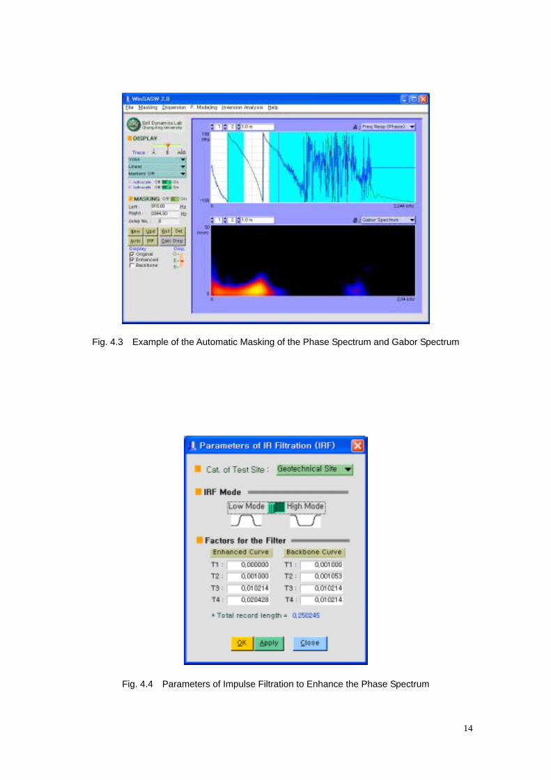
Fig. 4.3 Example of the Automatic Masking of the Phase Spectrum and Gabor Spectrum

Fig. 4.4 Parameters of Impulse Filtration to Enhance the Phase Spectrum

14

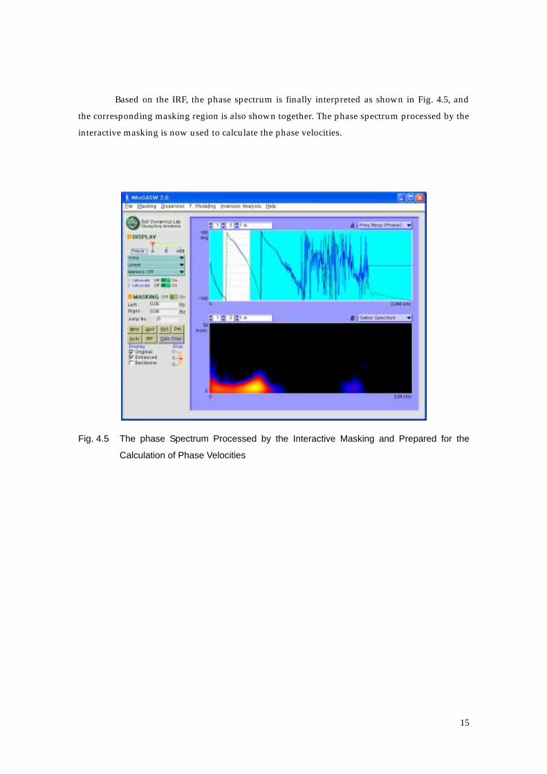
Based on the IRF, the phase spectrum is finally interpreted as shown in Fig. 4.5, and

the corresponding masking region is also shown together. The phase spectrum processed by the

interactive masking is now used to calculate the phase velocities.

Fig. 4.5 The phase Spectrum Processed by the Interactive Masking and Prepared for the

Calculation of Phase Velocities

15

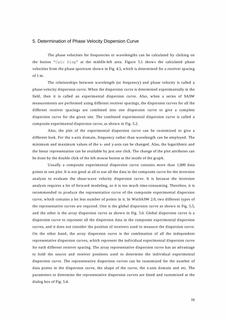
5. Determination of Phase Velocity Dispersion Curve The phase velocities for frequencies or wavelengths can be calculated by clicking on

the button “Calc Disp” at the middle-left area. Figure 5.1 shows the calculated phase

velocities from the phase spectrum shown in Fig. 4.5, which is determined for a receiver spacing

of 1 m.

The relationships between wavelength (or frequency) and phase velocity is called a

phase-velocity dispersion curve. When the dispersion curve is determined experimentally in the

field, then it is called an experimental dispersion curve. Also, when a series of SASW

measurements are performed using different receiver spacings, the dispersion curves for all the

different receiver spacings are combined into one dispersion curve to give a complete

dispersion curve for the given site. The combined experimental dispersion curve is called a

composite experimental dispersion curve, as shown in Fig. 5.2.

Also, the plot of the experimental dispersion curve can be customized to give a

different look. For the x-axis domain, frequency rather than wavelength can be employed. The

minimum and maximum values of the x- and y-axis can be changed. Also, the logarithmic and

the linear representation can be available by just one click. The change of the plot attributes can

be done by the double click of the left mouse button at the inside of the graph.

Usually a composite experimental dispersion curve contains more than 1,000 data

points in one plot. It is not good at all to use all the data in the composite curve for the inversion

analysis to evaluate the shear-wave velocity dispersion curve. It is because the inversion

analysis requires a lot of forward modeling, so it is too much time-consuming. Therefore, it is

recommended to produce the representative curve of the composite experimental dispersion

curve, which contains a lot less number of points in it. In WinSASW 2.0, two different types of

the representative curves are required. One is the global dispersion curve as shown in Fig. 5.5,

and the other is the array dispersion curve as shown in Fig. 5.6. Global dispersion curve is a

dispersion curve to represent all the dispersion data in the composite experimental dispersion

curves, and it does not consider the position of receivers used to measure the dispersion curve.

On the other hand, the array dispersion curve is the combination of all the independent

representative dispersion curves, which represent the individual experimental dispersion curve

for each different receiver spacing. The array representative dispersion curve has an advantage

to hold the source and receiver positions used to determine the individual experimental

dispersion curve. The representative dispersion curves can be customized for the number of

data points in the dispersion curve, the shape of the curve, the x-axis domain and etc. The

parameters to determine the representative dispersion curves are listed and customized at the

dialog box of Fig. 5.4.

16

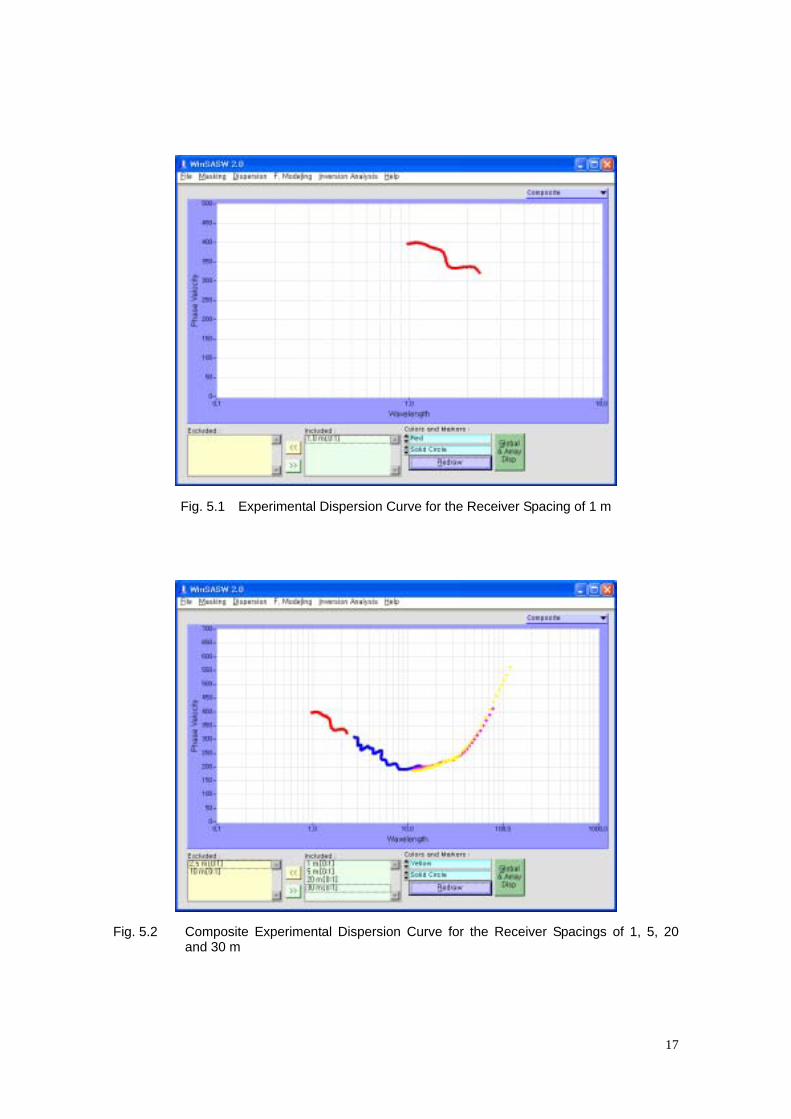
Fig. 5.1 Experimental Dispersion Curve for the Receiver Spacing of 1 m

Fig. 5.2 Composite Experimental Dispersion Curve for the Receiver Spacings of 1, 5, 20

and 30 m

17

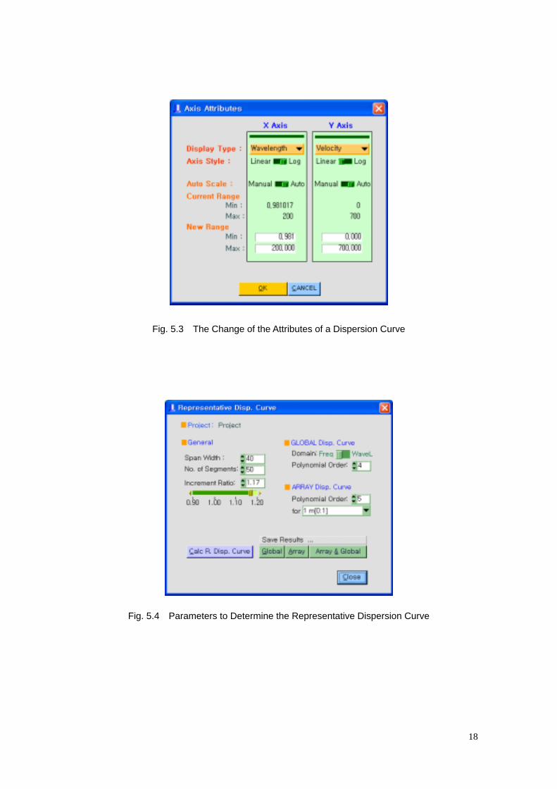
Fig. 5.3 The Change of the Attributes of a Dispersion Curve

Fig. 5.4 Parameters to Determine the Representative Dispersion Curve

18

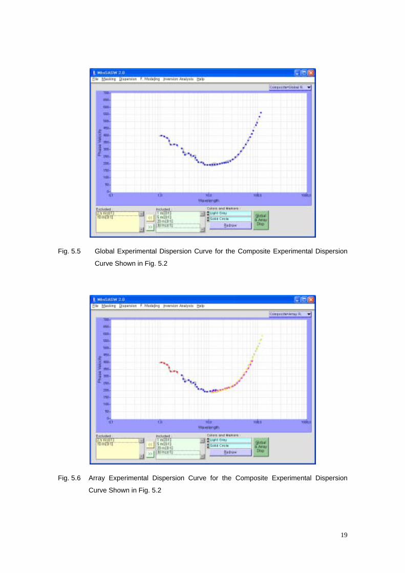
Fig. 5.5 Global Experimental Dispersion Curve for the Composite Experimental Dispersion

Curve Shown in Fig. 5.2

Fig. 5.6 Array Experimental Dispersion Curve for the Composite Experimental Dispersion

Curve Shown in Fig. 5.2

19

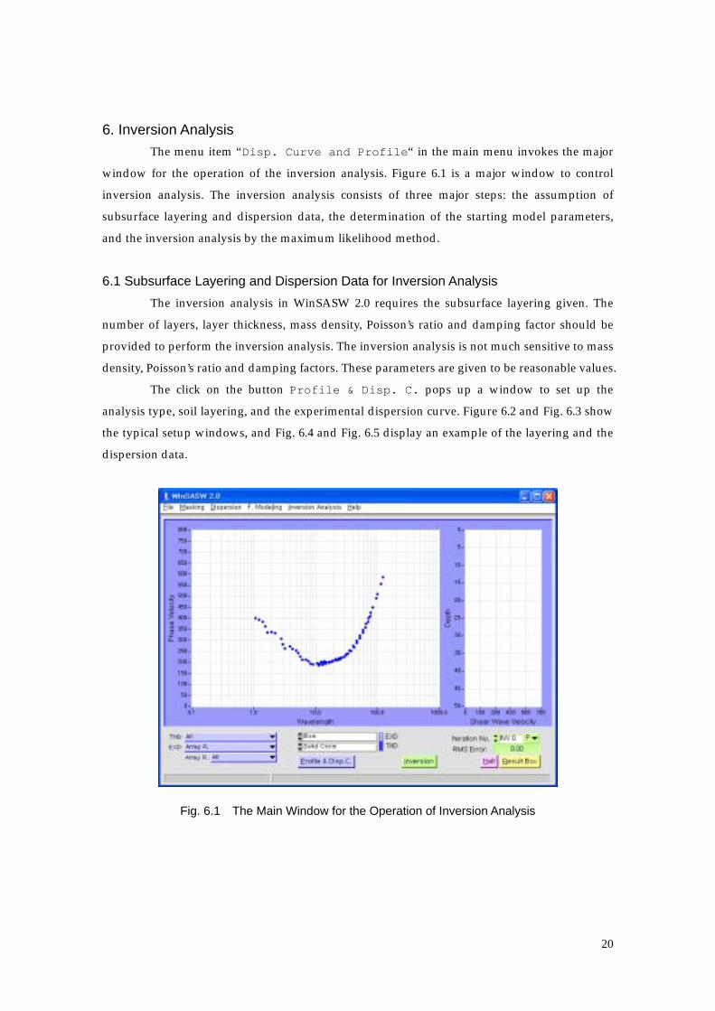
6. Inversion Analysis The menu item “Disp. Curve and Profile“ in the main menu invokes the major

window for the operation of the inversion analysis. Figure 6.1 is a major window to control

inversion analysis. The inversion analysis consists of three major steps: the assumption of

subsurface layering and dispersion data, the determination of the starting model parameters,

and the inversion analysis by the maximum likelihood method.

6.1 Subsurface Layering and Dispersion Data for Inversion Analysis The inversion analysis in WinSASW 2.0 requires the subsurface layering given. The

number of layers, layer thickness, mass density, Poisson’s ratio and damping factor should be

provided to perform the inversion analysis. The inversion analysis is not much sensitive to mass

density, Poisson’s ratio and damping factors. These parameters are given to be reasonable values.

The click on the button Profile & Disp. C. pops up a window to set up the

analysis type, soil layering, and the experimental dispersion curve. Figure 6.2 and Fig. 6.3 show

the typical setup windows, and Fig. 6.4 and Fig. 6.5 display an example of the layering and the

dispersion data.

Fig. 6.1 The Main Window for the Operation of Inversion Analysis

20

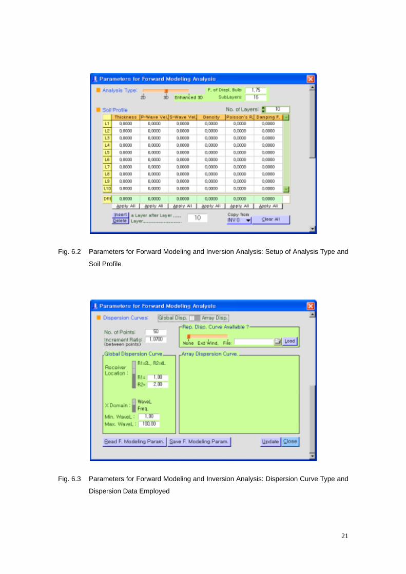
Fig. 6.2 Parameters for Forward Modeling and Inversion Analysis: Setup of Analysis Type and

Soil Profile

Fig. 6.3 Parameters for Forward Modeling and Inversion Analysis: Dispersion Curve Type and

Dispersion Data Employed

21

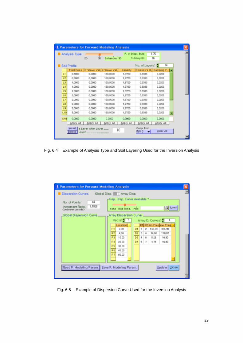
Fig. 6.4 Example of Analysis Type and Soil Layering Used for the Inversion Analysis

Fig. 6.5 Example of Dispersion Curve Used for the Inversion Analysis

22

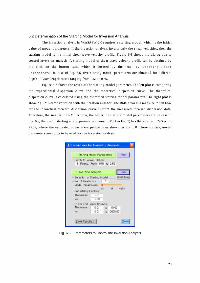
6.2 Determination of the Starting Model for Inversion Analysis The inversion analysis in WinSASW 2.0 requires a starting model, which is the initial

value of model parameters. If the inversion analysis inverts only the shear velocities, then the

starting model is the initial shear-wave velocity profile. Figure 6.6 shows the dialog box to

control inversion analysis. A starting model of shear-wave velocity profile can be obtained by

the click on the button Run, which is located by the text “1. Starting Model

Parameters.” In case of Fig. 6.6, five starting model parameters are obtained for different

depth-to-wavelength ratios ranging from 0.51 to 0.59.

Figure 6.7 shows the result of the starting model parameter. The left plot is comparing

the experimental dispersion curve and the theoretical dispersion curve. The theoretical

dispersion curve is calculated using the estimated starting model parameters. The right plot is

showing RMS-error variation with the iteration number. The RMS error is a measure to tell how

far the theoretical forward dispersion curve is from the measured forward dispersion data.

Therefore, the smaller the RMS error is, the better the starting model parameters are. In case of

Fig. 6.7, the fourth starting model parameter (named SMP4 in Fig. 7) has the smallest RMS error,

25.57, where the estimated shear wave profile is as shown in Fig. 6.8. These starting model

parameters are going to be used for the inversion analysis.

Fig. 6.6 Parameters to Control the Inversion Analysis

23

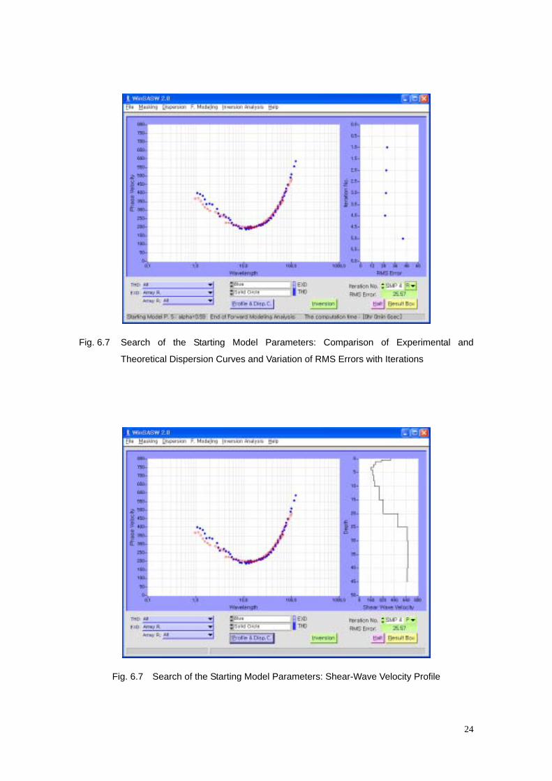
Fig. 6.7 Search of the Starting Model Parameters: Comparison of Experimental and

Theoretical Dispersion Curves and Variation of RMS Errors with Iterations

Fig. 6.7 Search of the Starting Model Parameters: Shear-Wave Velocity Profile

24

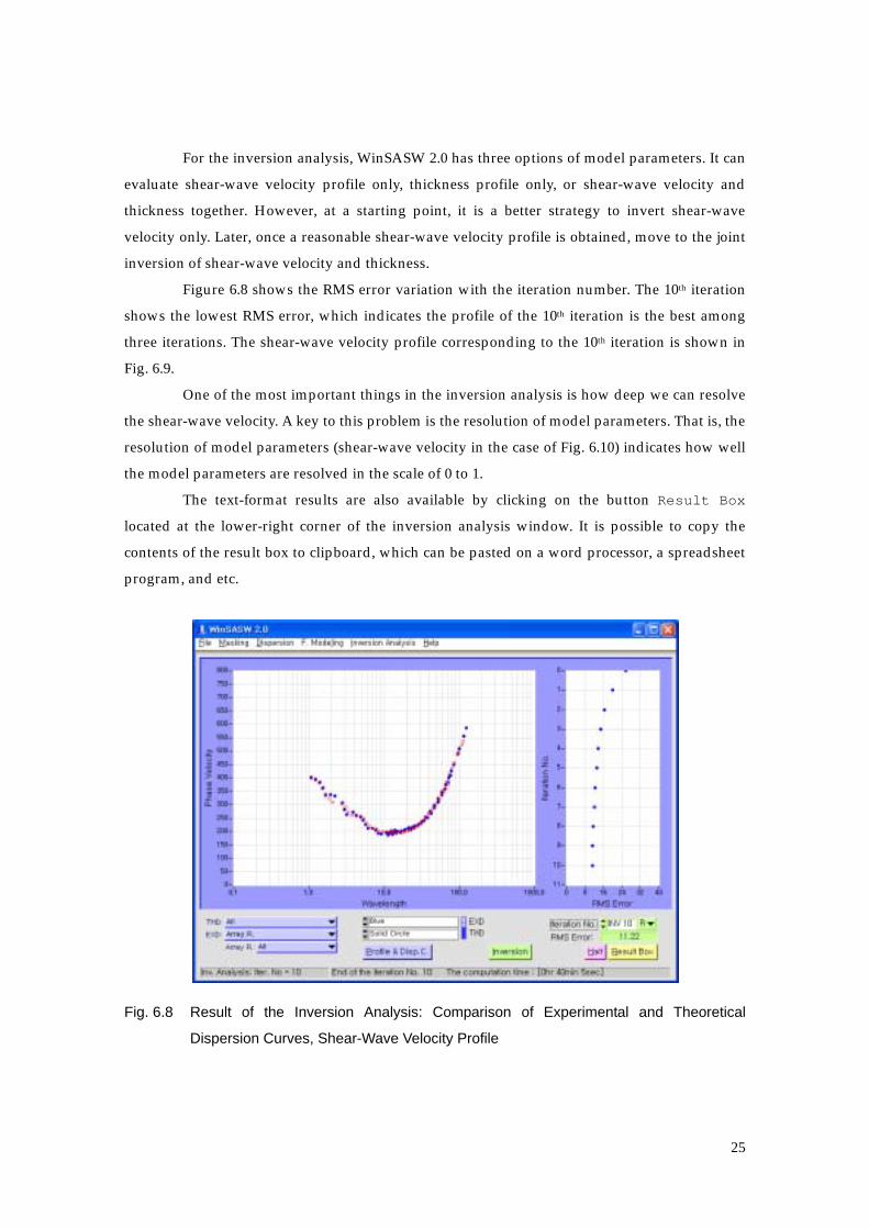
For the inversion analysis, WinSASW 2.0 has three options of model parameters. It can

evaluate shear-wave velocity profile only, thickness profile only, or shear-wave velocity and

thickness together. However, at a starting point, it is a better strategy to invert shear-wave

velocity only. Later, once a reasonable shear-wave velocity profile is obtained, move to the joint

inversion of shear-wave velocity and thickness.

Figure 6.8 shows the RMS error variation with the iteration number. The 10th iteration

shows the lowest RMS error, which indicates the profile of the 10th iteration is the best among

three iterations. The shear-wave velocity profile corresponding to the 10th iteration is shown in

Fig. 6.9.

One of the most important things in the inversion analysis is how deep we can resolve

the shear-wave velocity. A key to this problem is the resolution of model parameters. That is, the

resolution of model parameters (shear-wave velocity in the case of Fig. 6.10) indicates how well

the model parameters are resolved in the scale of 0 to 1.

The text-format results are also available by clicking on the button Result Box

located at the lower-right corner of the inversion analysis window. It is possible to copy the

contents of the result box to clipboard, which can be pasted on a word processor, a spreadsheet

program, and etc.

Fig. 6.8 Result of the Inversion Analysis: Comparison of Experimental and Theoretical

Dispersion Curves, Shear-Wave Velocity Profile

25

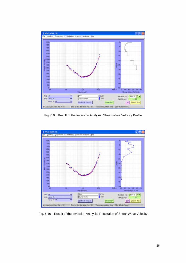
Fig. 6.9 Result of the Inversion Analysis: Shear-Wave Velocity Profile

Fig. 6.10 Result of the Inversion Analysis: Resolution of Shear-Wave Velocity

26

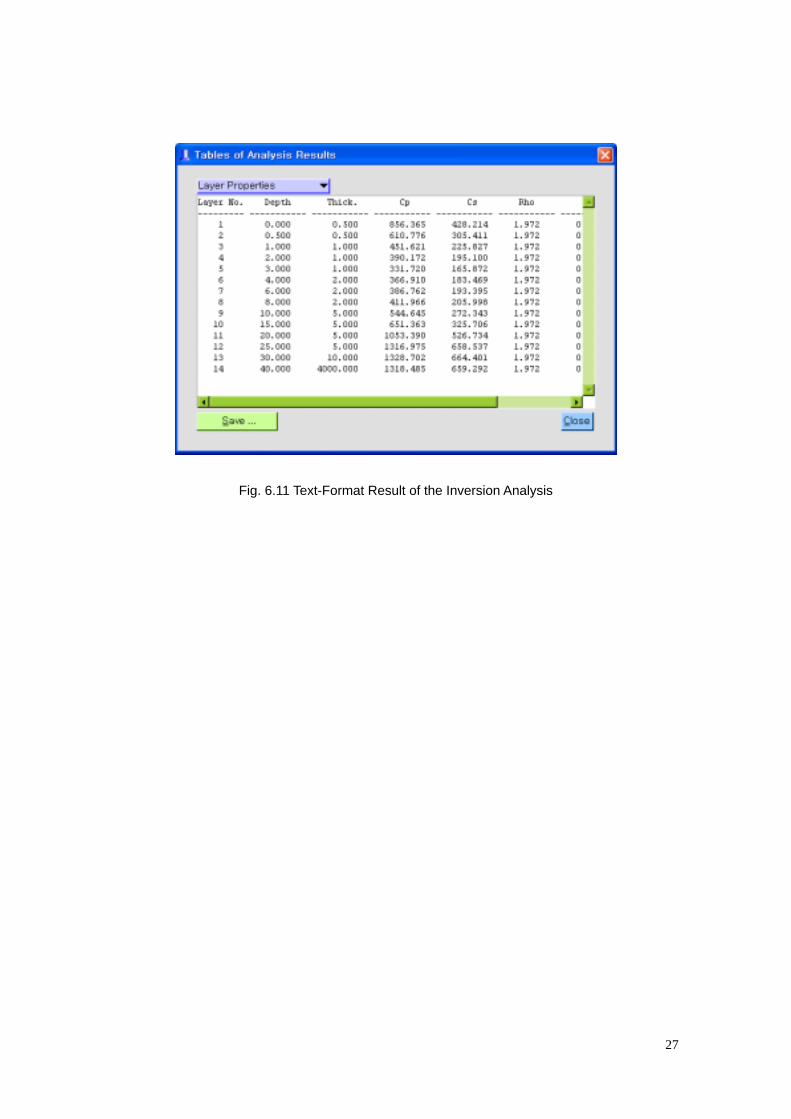
Fig. 6.11 Text-Format Result of the Inversion Analysis

27

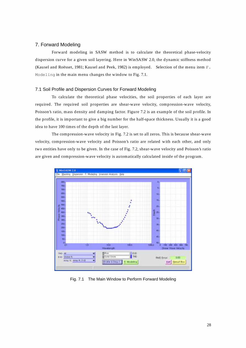
7. Forward Modeling Forward modeling in SASW method is to calculate the theoretical phase-velocity

dispersion curve for a given soil layering. Here in WinSASW 2.0, the dynamic stiffness method

(Kausel and Roësset, 1981; Kausel and Peek, 1982) is employed. Selection of the menu item F.

Modeling in the main menu changes the window to Fig. 7.1.

7.1 Soil Profile and Dispersion Curves for Forward Modeling To calculate the theoretical phase velocities, the soil properties of each layer are

required. The required soil properties are shear-wave velocity, compression-wave velocity,

Poisson’s ratio, mass density and damping factor. Figure 7.2 is an example of the soil profile. In

the profile, it is important to give a big number for the half-space thickness. Usually it is a good

idea to have 100 times of the depth of the last layer.

The compression-wave velocity in Fig. 7.2 is set to all zeros. This is because shear-wave

velocity, compression-wave velocity and Poisson’s ratio are related with each other, and only

two entities have only to be given. In the case of Fig. 7.2, shear-wave velocity and Poisson’s ratio

are given and compression-wave velocity is automatically calculated inside of the program.

Fig. 7.1 The Main Window to Perform Forward Modeling

28

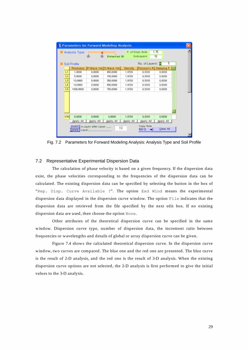
Fig. 7.2 Parameters for Forward Modeling Analysis: Analysis Type and Soil Profile

7.2 Representative Experimental Dispersion Data The calculation of phase velocity is based on a given frequency. If the dispersion data

exist, the phase velocities corresponding to the frequencies of the dispersion data can be

calculated. The existing dispersion data can be specified by selecting the button in the box of

“Rep. Disp. Curve Available ?”. The option Exd Wind means the experimental

dispersion data displayed in the dispersion curve window. The option File indicates that the

dispersion data are retrieved from the file specified by the next edit box. If no existing

dispersion data are used, then choose the option None.

Other attributes of the theoretical dispersion curve can be specified in the same

window. Dispersion curve type, number of dispersion data, the increment ratio between

frequencies or wavelengths and details of global or array dispersion curve can be given.

Figure 7.4 shows the calculated theoretical dispersion curve. In the dispersion curve

window, two curves are compared. The blue one and the red one are presented. The blue curve

is the result of 2-D analysis, and the red one is the result of 3-D analysis. When the existing

dispersion curve options are not selected, the 2-D analysis is first performed to give the initial

values to the 3-D analysis.

29

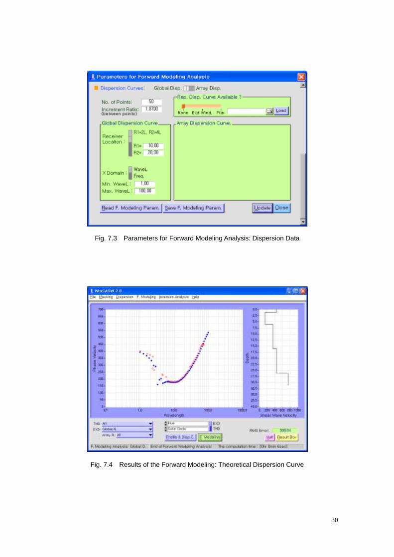
Fig. 7.3 Parameters for Forward Modeling Analysis: Dispersion Data

Fig. 7.4 Results of the Forward Modeling: Theoretical Dispersion Curve

30

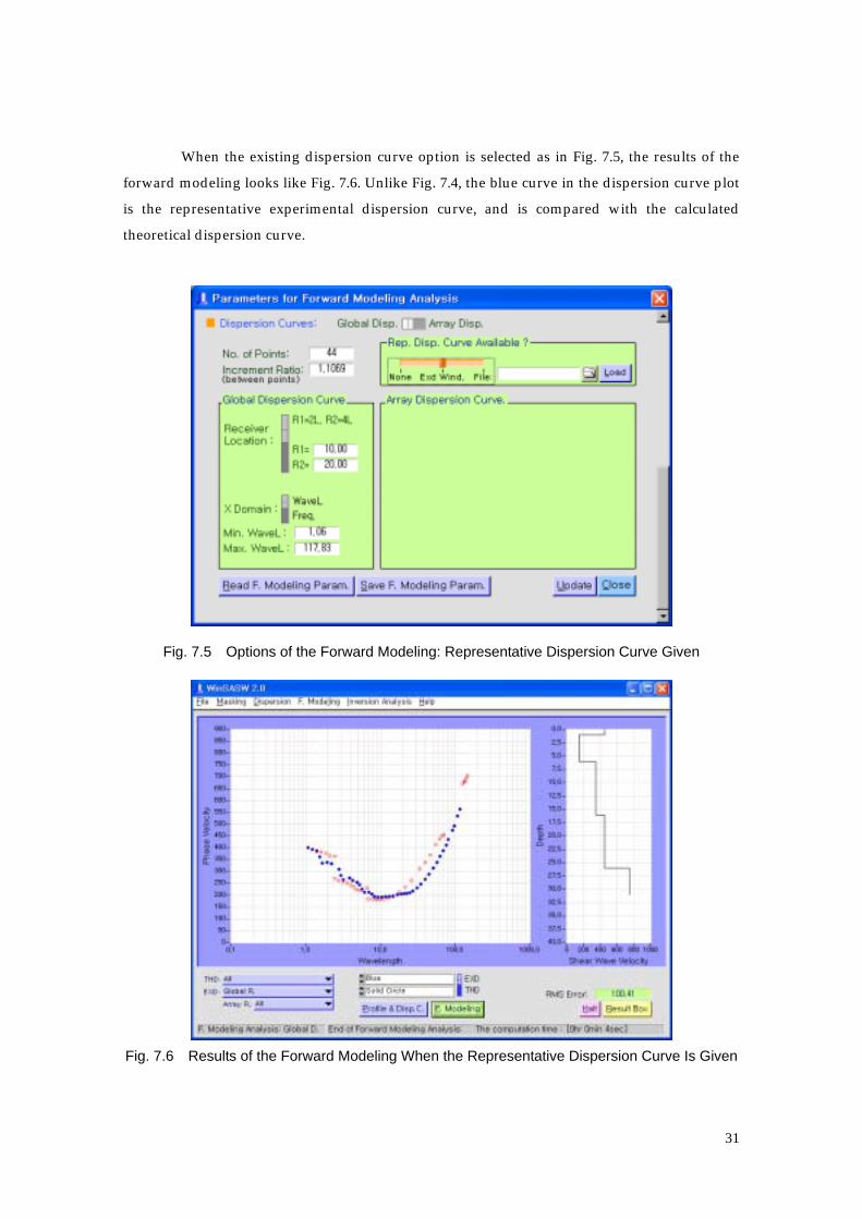
When the existing dispersion curve option is selected as in Fig. 7.5, the results of the

forward modeling looks like Fig. 7.6. Unlike Fig. 7.4, the blue curve in the dispersion curve plot

is the representative experimental dispersion curve, and is compared with the calculated

theoretical dispersion curve.

Fig. 7.5 Options of the Forward Modeling: Representative Dispersion Curve Given

Fig. 7.6 Results of the Forward Modeling When the Representative Dispersion Curve Is Given

31

When the array dispersion curve is chosen as a analysis type, the section for an array

dispersion curve is visible as in Fig. 7.7. In the section of the array dispersion curve, information

on receivers and array dispersion curves should be provided. In the case of Fig. 7.7, information

on the existing array dispersion curve is employed. The results of forward modeling analysis for

the options given in Fig. 7.7 look like Fig. 7.8.

Fig. 7.7 Options of Forward Modeling Analysis for the Array Dispersion Curve

Fig. 7.8 Results of Forward Modeling Analysis for the Array Dispersion Curve Option

32

33

References

1. Foinquinos M. R. (1991). "Analytical study and inversion for the spectral analysis of surface

waves method." Thesis, the University of Texas at Austin.

2. Heisey, J. S., Stokoe, K.H., II, Hudson, W. R. and Meyer, A. H. (1982). "Determination of in

situ shear wave velocities from Spectral-Analysis-of-Surface-Waves." Research Report No.

256-2 Center for Transportation Research, The University of Texas at Austin.

3. Joh, S.-H. (1996). "Advances in data interpretation technique for Spectral-Analysis-of-

Surface-Waves(SASW) measurements." Ph.D. Dissertation, the University of Texas at Austin,

Austin, Texas, U.S.A.

4. Joh, S.-H. (1996). FIT7: Program for Forward Modeling Analysis, Inversion Analysis and

Time Trace Generation, the University of Texas at Austin, Austin, Texas, U.S.A.

5. Kausel, E. and Roesset, J. M. (1981). "Stiffness matrices for layered soils." Bull. Seismol. Soc.

Am., vol. 71, pp. 1743-1761.1. Nazarian, S. and Stokoe, K. H., II (1984). "Use of surface waves

in pavement evaluation." Transportation Research Record, 1070, pp. 132-144.

6. Kausel, E. and Peek, R. (1982). "Dynamic loads in the interior of a layered stratum: an

explicit solution." Bull. Seismol. Soc. Am., vol. 72, pp. 1259-1508.

7. Tarantola, A. (1987). Inverse problem theory: Methods for data fitting and model parameter

estimation. 600 pp., New York, Elsevier.