Data management using SPSS – part 1

Laine Ruus

(datalib@ed.ac.uk)

University of Edinburgh. Data Library

2016-11-15

Part Content Paragraphs

1 Introduction 1 - 4

1 Data log file and configuring SPSS 5 - 14

1 Creating an SPSS system file 15 - 34

1 Descriptive statistics – checking the data 35 - 43

2 Common variable transformations 44 - 54

3 Common file transformations 55 - 62

3 Getting your data out of SPSS 63 - 69

Appendix A: Some favourite on-line resources

Appendix B: Selected limitations on file, variable and value names

Appendix C: Common file and variable transformations and their corresponding SPSS commands

Appendix D: SPSS read and write commands by input/output format

The objective of this course is to introduce you to some techniques for using SPSS as well as other

tools to support your data management (RDM) activities during the course of your research. It is not

about doing statistical analysis using SPSS, but rather how to transform your data, and document

your data management activities, in the context of using SPSS for your analyses.

[Michael] Cavaretta said: “We really need better tools so we can spend less time on data wrangling

and get to the sexy stuff.” Data wrangling is cleaning data, connecting tools and getting data into a

usable format; the sexy stuff is predictive analysis and modeling. Considering that the first is

sometimes referred to as "janitor work," you can guess which one is a bit more enjoyable.

In CrowdFlower's recent survey, we found that data scientists spent a solid 80% of their time

wrangling data. Given how expensive of [sic] a resource data scientists are, it’s surprising there are

not more companies in this space.

Source: Biewald, Lukas Opinion: The data science ecosystem part 2: Data wrangling. Computerworld Apr 1, 2015

http://www.computerworld.com/article/2902920/the-data-science-ecosystem-part-2-data-wrangling.html

1. When embarking on the exploration of a new research question, after the literature review, and

the formulation of preliminary hypotheses, the next task is generally to begin to identify (a) what

variables you need in order to test your hypotheses, and run your models (b) what datafiles (if

any) are already available that contain those variables, or whether and how to collect new data,

and (c) what software package(s) has the statistical analysis routines and related capabilities

(data cleaning, data transformations, etc) that you require.

2. The questions you need to be able to answer, vis-à-vis any software you decide to use, are (a)

does the software support the statistical analyses that are most appropriate for my research

question and data? (b) how good/defensible are the measures that the software will produce?

(c) will it support the data exploration and data cleaning/transformations I need to perform? (d)

how will I get my data into the software (ie what file formats can it read)?, and (e) equally

importantly, how can I get my data out of that software (along with any transformations,

computations etc) so that I can read it into other software for other analyses, or store it in a

software-neutral format for the longer term? This workshop assumes you have decided to use

SPSS for your analyses, at least in part. This document, and the exercises, are based on SPSS

versions 21/22.

3. Advantages to SPSS include:

flexible input capabilities, (eg hierarchical data formats)

flexible output capabilities

metadata management capabilities, such as variable and value labels, missing values etc

data recoding and computing capabilities

intuitive command names, for the most part

produces statistical measures comparable to those from SAS. Stata, etc.

good documentation and user support groups (see Appendix A)

Disadvantages to SPSS include:

• doesn’t do all possible statistical procedures (but then, no statistical package does)

• does not handle long question text well

• allows very long variable names (>32 characters) which cannot be read by other

statistical packages

• default storage formats for data and output log files are software-dependant (but this is

also true for most statistical packages)

4. The data being used in this exercise are a subset of variables and cases from:

Sandercock, Peter; Niewada, Maciej; Czlonkowska, Anna. (2014). International Stroke Trial

database (version 2), [Dataset]. University of Edinburgh, Department of Clinical Neurosciences.

http://dx.doi.org/10.7488/ds/104.

The citation specifies that this is ‘version 2’. An important part of data management is keeping

track of dataset versions and documenting the changes that have happened between versions,

especially of your own data. The web page describing the data set has that information.

You should have access to the following files in the accompanying Mantra .zip file:

- ist_corrected_uk1.csv – a comma-delimited file, which we will convert to an SPSS system file

- ist_corrected_uk2.sav – an SPSS system file from which we will add variables

- ist_corrected_eu15.sav – an SPSS system file from which we will add cases

- ist_labels1.sps – an SPSS syntax file to add variable-level metadata to the SPSS file

- IST_logfile.xlsx – a sample log file in Excel format

Data log file

5. As part of managing your data it is important to create your own documentation as you work through your analyses. It is good practice to set up a Data log right at the start of a project, to keep track of eg the locations of versions of datafiles and documentation, notes about variables and values, and file and variable transformations, output log files, etc. This is information that is easily forgotten, within days, much less months, and should you make a mistake, will help you backtrack to a good version of your dataset.

The Data log file will also help you, at the end of your project, to identify what versions of the data file(s), syntax files, and output files to keep, and which can be discarded. At a minimum, you should keep the original and the final versions of the datafile(s), as well as the syntax files or output files which include the syntax, for all transformations, as well, of course, as keeping the data log file. Keeping these files, at a minimum, will assist you to defend your transformations and analyses, should they be queried in the future.

6. The software you choose in which to manage your data log is a matter of personal choice. Some researchers prefer to use a word processor (eg MS Word), others to use a format-neutral text editor, such as Notepad or EditPad Lite, and yet others prefer the table handling and sorting capability of Microsoft Excel (see the file ‘IST_logfile.xlsx). Open a new Excel spreadsheet, and eg on sheet 1, enter, in successive columns, the following suggested fields:

- Current date (YYYYMMDD) - The input file location and format (‘format’ is especially important if you are working in a

MacOS environment, which does not require format based filename extensions). The first entry should be where you obtained the data [if doing secondary analysis]

- The output file location, name and format - A comment as to what was done between input and output. - Rename the sheet, eg ‘data log’ – we will be adding more information later - Before you do anything else, save the file (assign a location and name that you will

remember), but leave it open.

Hint: in order to get the correct path and filename of a file in a Windows environment, locate the file in Windows Explorer, and.

Alternative 1: Click in the address bar showing the path at the top of the Windows Explorer window. The display will toggle between read-friendly display, and the full path display. Copy and paste the full path display, and type the filename, or Alternative 2: Click on the file to select it. Then right-click, and select ‘Properties’. The exact path will be displayed in the ‘Location’ field of the properties window, and the filename in the first dialogue box. Both path and filename can be copied and pasted into the data log.

7. It is good practice to assume that you may not always be using SPSS, or the same version of SPSS, for your analyses. You may need to migrate data from/to different computing environments (Windows, Mac, Linux/Unix) and/or different statistical software, because no statistical package supports all types of analysis (SAS, Stata, R, etc). Therefore you also need to be aware of constraints on lengths of file names, variable names, and other metadata such as variable labels, value labels, and missing values codes in different operating systems and software packages, some of which are listed in Appendix B.

8. Note: Especially if you are in the habit of working in different computer environments, it is not recommended that you use blanks in file or directory/folder names. Different operating systems treat embedded blanks differently. Instead, use eg underscores or CamelCase to separate words to make names more readable. Ie, not ‘variable list.xls’ but ‘variable_list.xls’ or ‘VariableList.xls’.

Running SPSS and configuring options

9. Open SPSS through your programs menu: Start > IBM SPSS Statistics [nn]. If a dialog box appears asking you whether you wish to open an existing data source, click ‘Cancel’. When you run SPSS in Windows, one window is opened automatically: – a Data editor window - empty until you open a data file or begin to enter variable values, after which it will have two views, a Variable View and a Data View, Once you have loaded a data file, or issued a command from the drop-down menus, a second window will open: – an Output window, to which output from your commands and error messages will be written. Additional windows which can be opened from File > New1 or File > Open (if they already exist) are: - a Syntax window, in which you can ‘paste’ syntax from the drop-down menu choices, enter

syntax directly, edit and run syntax, - a Script window, in which you can enter, and edit, Python scripts.

Three additional windows, in addition to dialogue windows etc., may or may not open depending on the procedures you are running: (a) a Pivot table editor window, (b) a Chart editor window, and (c) a Text output editor window.

10. Before starting to read data, you should make some changes to the SPSS environment defaults. Select Edit > Options. The Options box has several tabs.

1 Unless otherwise specified, all following Menu > [Submenu] > Item references are to drop-down menus in

the SPSS interface.

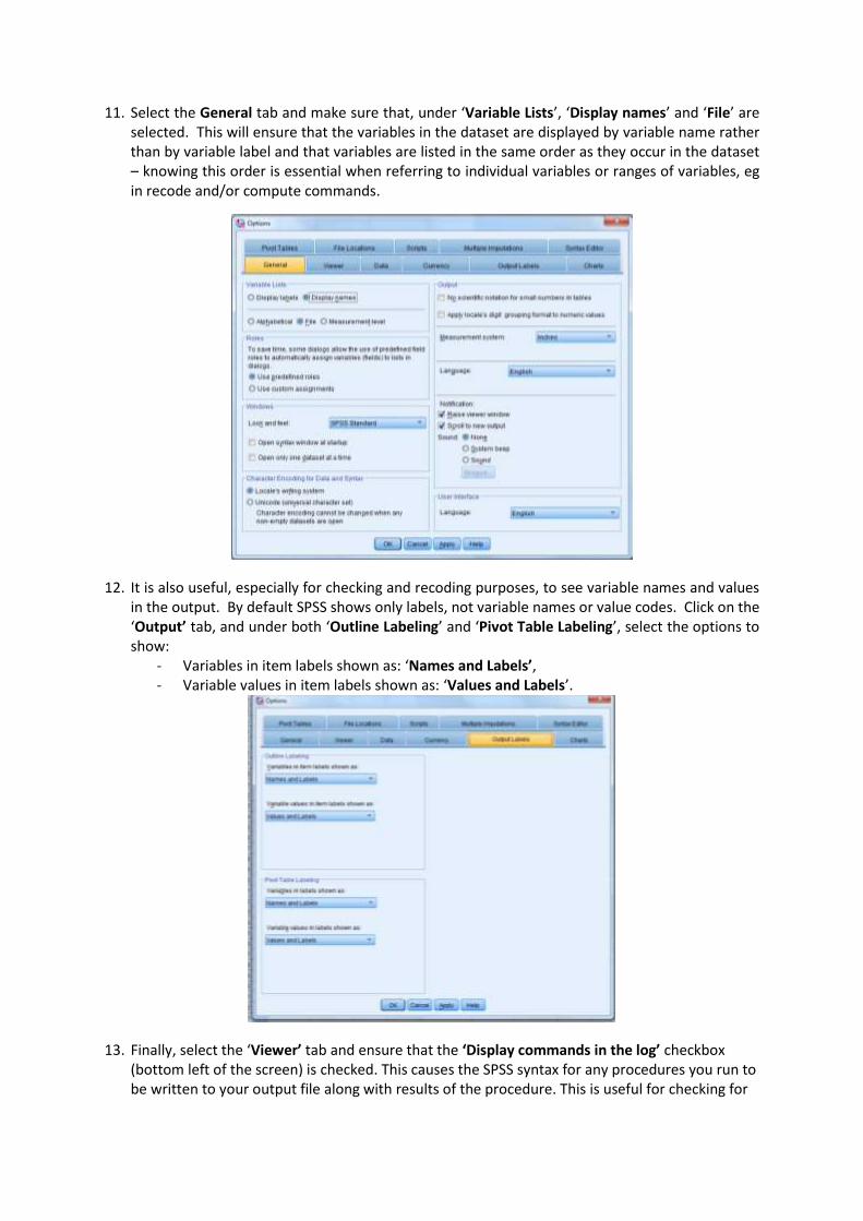
11. Select the General tab and make sure that, under ‘Variable Lists’, ‘Display names’ and ‘File’ are selected. This will ensure that the variables in the dataset are displayed by variable name rather than by variable label and that variables are listed in the same order as they occur in the dataset – knowing this order is essential when referring to individual variables or ranges of variables, eg in recode and/or compute commands.

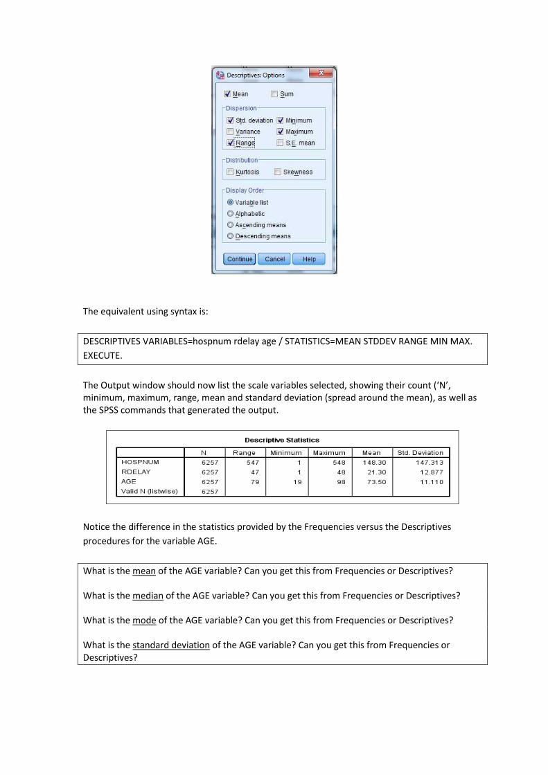
12. It is also useful, especially for checking and recoding purposes, to see variable names and values in the output. By default SPSS shows only labels, not variable names or value codes. Click on the ‘Output’ tab, and under both ‘Outline Labeling’ and ‘Pivot Table Labeling’, select the options to show:

- Variables in item labels shown as: ‘Names and Labels’, - Variable values in item labels shown as: ‘Values and Labels’.

13. Finally, select the ‘Viewer’ tab and ensure that the ‘Display commands in the log’ checkbox (bottom left of the screen) is checked. This causes the SPSS syntax for any procedures you run to be written to your output file along with results of the procedure. This is useful for checking for

errors, as well as as a reminder of the details of recodes and other variable transformations, etc. Click ‘OK’ to save the changes.

Examine the data file

14. First we will look at one common type of external, raw data file, in this case a comma-delimited

file, with extension ‘.csv’. Run Notepad++ and open the file ‘ist_corrected_uk1.csv’ (in Libraries

> Documents > SPSS Files).

Jakobsen's Law. “If Excel can misinterpret your data, it will. And usually in the worst possible way”. <http://asiapacificparllibs.org/wp-content/uploads/sites/2/2015/12/Australia-Sam-Spencer-Parliamentary-Data-

Management.pdf>

Note: Do not use Excel to open the file. Notepad++ (or Notepad) will display the file in a format-

neutral way, in a non-proportional font, so that we can see what the file really contains, rather

than what Excel interprets the content to be.

In this data file, each unit of observation (row) represents a stroke patient in the IST sample: patients with suspected acute ischaemic stroke entering participating hospitals in the early 1990s, randomised within 48 hours of symptom onset. The variables in the rows describe characteristics of the patients, their symptoms, treatment, and outcomes. This particular subset contains patients from the UK only, and only those variables describing the patient at the time of enrollment in the trial, and at the 14 day follow-up.

This a simple flat .csv file, with one unit of observation (case) in each row, and all the variables relating to that case, in the same order, making up the row, separated by commas. Using the cursor to move around the file, determine:

How many cases (rows) are there in this dataset? (Hint: scroll down and click on the last row. The

number of the row is given by Ln in the bottom ribbon of the screen)2

Is there a row of variable names as the first row? Y|N

Are there blanks in the data, between commas (the delimiters)? Y|N

Are there blanks embedded among other characters in individual fields? Y|N

Are comment fields and/or other alphabetic variables enclosed in quotation marks? Y|N

Are full stops or commas used to indicate the position of the decimal in real numbers?

NB: SPSS requires that all decimal places be indicated by full stops.

2 To enable the display of the number of lines and line length in Notepad (as opposed to Notepad++),

turn off Format > Word Wrap and click on the last line of the file. The line number of the last line will

be displayed at the bottom of the screen.

Note: Rules for variable names in SPSS: (a) variable names must be unique in the data set, (b) must

start with a letter, (c) be short, about 8 characters is best (d) must not contain spaces but may

contain a few special characters such as full stop, underscore, and the characters $, #, and @, (e) should

not end with a full stop, and (f) should reflect the content of the variable. Variable names beginning

with a ‘$’ (eg. $CASEID, $CASENUM, $DATE, $SYSMIS, etc) are system variables – do not use these as

regular variable names. Also, do not use names of SPSS commands as variable names.

Not variable names:

Patient #

Cancer Diag

# chemo cycle

7. On a scale of 1 to 5, where 1 is ‘disagree’ and 5 is ‘agree’, please tell us … [etc]

Good variable names:

Patient# or Patient_no

CancerDiag or Cancer_Diag

chemo_cycle_no or ChemoCycleNo

q7 or agree7 or disagree7

Creating an SPSS system file

15. In common with most statistical packages, SPSS needs a variety of information in order to read a raw numeric data file: (a) the data, and (b) instructions as to how to read the data. In its simplest form, SPSS reads a raw data file (eg ‘ist_corrected_uk1.csv’), a syntax file (eg ‘ist_labels1.sps’), and using the input instructions in the data and syntax files, converts data and metadata into its preferred format, a system file (extension ‘.sav’), which exists only during your current SPSS session unless you save it.

16. From the SPSS drop-down menus, select File > Read Text Data. In the Open Data window,

browse Libraries > Documents > SPSS files to locate and open the ‘ist_corrected_uk1.csv’ file,

and finally click on ‘Open’. NB This will not work if the file is already open in Excel.

This will launch the SPSS Text Import Wizard, a 6-step sequence that will request instructions

from you as to how to read the .csv file. Remember the answers you gave to the questions in

paragraph 13, above, as you work through the steps, particularly in step 2 (yes, you have a row

of headers) and step 4 (no, a Space is NOT a field delimiter in this file, only the comma is, and no

there is no ‘text qualifier’).

Syntax: ist_labels1.sps Data: ist_corrected_uk1.csv

SPSS

SPSS system file

SPSS will use your input as well as the data in the first 200 cases to automatically compile a

format specification for the file. NB if any field is longer in later cases than in any instance in the

first 200 cases, the content of the longer fields will be truncated.

17. You should, at the end of the Import Wizard process, have:

A Data Editor : Data View window which contains a spreadsheet-like display of the data:

A Data Editor : Variable View window contains a list of variable names and their associated

characteristics :

An Ouput window listing the syntax SPSS used to read the input data file:

….LOTS OF LINES DELETED

18. SPSS can read (and write) a variety of formats. See Appendix D for a list of software dependant

formats and the SPSS commands to read and write them. SPSS can also read more complex file

formats, such as multiple records per case, mixed files, hierarchical files, etc.

An SPSS syntax file to read a raw data files contains instructions to SPSS re (a) what file to read

(FILE=”…”) and (b) how to read it (TYPE=TXT), as well as (c) a data list statement (VARIABLES=…),

(c) variable labels statement, (e) value labels statement, and (f) missing data statement. Thus far,

we have only provided information for (a) through (c), and later will add (d) through (f).

Data list statement for a fixed field format file:

Data list statement for a delimited file with one case per row, and no column headers:

Checking and saving the output

19. Checking: (1) check the Output window for Error messages, (2) click on the Data Editor window,

and check both the Variable View, and the Data View, for anything that looks not quite right. If

there are errors, try to figure out what they are. Normally, fix the first error first, and then rerun

the job – errors often have a cascading effect, and fixing the first can eliminate later errors.

scroll through the Data View window, up-down and sideways, to CHECK that each variable

contains the same type of coding, eg there are no words in a column with numeric codes, etc.

How many cases have been read? Is this the same as the number of rows in the raw data?

Are there the same number of variable names and columns of data? (SPSS assigns default names ‘VAR[nnn]’ to unnamed variables.)

Does each column appear to contain the same type and coding range of data?

Have variables containing embedded blanks, eg comment fields, been read correctly?

Do any variables (eg comment fields) appear to have been truncated?

Have numbers containing decimals been read correctly?

20. Saving the work so far

a. Save the SPSS system file. Select File > Save as and save the file with format ‘SPSS Statistics (*.sav)’. And record the location of this file in the Data log. One method to distinguish among versions of a file is to begin each filename with the YYYYMMDD of the date on which it was created, eg:

i. 20140921ist_corrected_uk1.sav

b. Save the Output file In current versions of SPSS, the Output Viewer is labelled ‘Output[n] [Document[n]] IBM SPSS Statistics Viewer’). It is the window in which output from your procedures is displayed, as well as the syntax that generated it (as a result of the options chosen in paragraph 13 above). The Output window should now contain the syntax SPSS used to read the .csv file. For data management purposes, this Output file is important documentation and your only record of what you have done to the file/variables and what the results were. Therefore, it is very important to keep these output files.

This output can be saved. By default the output file is saved as an SPSS-dependant format with default filename ‘Output[n]’, and the extension .spv (.spo in versions prior to SPSS18) which can only be read by SPSS; therefore, instead of saving it, use File > Export to convert it to a .txt, .html or .pdf format (which you will be able to read with other software), with a meaningful filename. And, of course, add this information to the Data log file.

c. Save the syntax file (if you created one): File > Save as. Note that an SPSS syntax file takes the default extension ‘.sps’, and is a flat text file, so readable by any text software.

d. Update the Data log file (Excel).

Using syntax

21. You can carry out most of your data analyses and variable transformations (including creating

new variables) in SPSS using drop-down menus. Alternatively, you can also analyse and

manipulate your data using SPSS command language (syntax), which you can save and edit in a

‘syntax file’, rather than using drop-down menus. For some procedures, syntax is actually easier

and more customiseable than using the menus.

22. You need syntax files when:

You want to make your analyses repetitive, i.e. easily reproducible on a different or

changed data set

You want to have the option of correcting some details in your analysis path while keeping the rest unchanged

Some operations are best automated in programming constructs, such as IFs or LOOPs

You want a detailed log of all your analysis steps, including comments

You need procedures or options which are available only with syntax

You want to save custom data transformations in order to use it them later in other analyses

You want to integrate your analysis in some external application which uses the power of SPSS for data processing Source: Raynald’s SPSS tools <http://spsstools.net/en/syntax/>

23. For example, if you discover that SPSS has truncated some data fields when reading in the .csv file, you can save the syntax to read the data file in a syntax file, edit it to increase the size of individual fields, and rerun it:

Double R-click in the Output window in the area of the syntax written by SPSS

Ctrl-C to save the content of the yellow-bounded box around the output

Menus: File > New > Syntax to open a new syntax window

Ctrl-V to copy the content of the yellow-bounded box from the Output to the Syntax window

The variable ‘DSIDEX’ in this data file is defined, based on the first 200 cases, as a 26 character string variable (A26). To increase the size of that variable to 50 characters, edit the syntax file to read ‘DSIDEX A50’. Then rerun the syntax to read in the raw data file again: click and drag to select the syntax file contents, from the DATA statement down to and including the full stop ‘.’ at the end of the file, or select Edit > Select All, and click on the large green arrowhead (the ‘Run’ icon) on the SPSS tool bar to run it. Then of course, you will need to check the new file as discussed above.

24. Advantages to using syntax:

• a handful of SPSS commands/subcommands are available via syntax but not via the drop-down menus, such as temporary, missing=include and manova

• for some procedures, syntax is actually easier and more flexible than using the menus. • you can perform with one click all the variable recoding/checking and labelling assignments

necessary for a variable • you can run the same set of syntax (cut and paste or edit) with different variables merely by

changing the variable names, and run or re-run it by highlighting just those commands you want to run, and then clicking on the Run icon.

• annotate the syntax file with COMMENTS as a reminder of what each set of commands does for future reference. COMMENTS will be included in your output files.

In the exercises that follow you will be using a mix of drop-down menus and syntax to work with

the dataset and to create new variables.

25. Rules to remember about SPSS syntax:

commands must start on a new line, but may start in any column (older versions: column ‘1’)

commands must end with a full stop (‘.’)

commands are not case sensitive. Ie ‘FREQS’ is the same as ‘freqs’

each line of command syntax should be less than 256 characters in length

subcommands usually start with a forward slash (‘/’)

add comments to syntax (preceded by asterisk ‘*’ or ‘COMMENT’, and ending with a full stop) before or after commands, but not in the middle of commands and their subcommands.

many commands may be truncated (to 3-4 letters), but variable names must be spelled out in full

26. Where do syntax files for reading in the data come from?

a. If you have collected your own data:

You should write your own syntax file as you plan, collect and code the data.

Some sites, such as the Bristol Online Surveys (BOS) site, will provide documentation as to what the questions and responses in your survey were, but you will have to reformat that information to SPSS specifications.

If you are doing secondary analysis, ie using data from another source:

data from a data archive, should also be accompanied by a syntax file or be a system file with the metadata already in it

If the data are from somewhere else, eg on the WWW, look to see if a syntax file is provided

Failing a syntax file, look for some other type of document that explains what is in each variable and how it is coded. You will then need to write your own syntax file.

And failing that, you should think twice about using the data, if you have no documentation as to how it was collected, coded, and what variables it contains, and how they are coded.

27. To generate syntax from SPSS:

a. If unsure about how to write a particular set of syntax, try to find the procedure in the drop-down menus

b. Many procedures have a ‘Paste‘ button beside the ‘OK’ button c. Clicking on the ‘Paste’ button will cause the syntax for the current procedure to be

written to the current syntax file, if you have one already open; If you do not have a syntax file open, SPSS will create one

d. Note: if you use the ‘Paste’ button, the procedure will not actually be run until you select the syntax (click-and-drag) and click the ‘Run’ button on the SPSS tool bar

Adding variable and value labels, and user-defined missing data codes

28. Common metadata management tasks in SPSS:

a. Rename variables b. Add variable labels c. Optimize variable labels for output d. Add value labels to coded values, eg ‘1’ and ‘2’ for ‘male’ and ‘female’ e. Optimize length and clarity of value labels for output f. Add missing data specifications, to avoid the inclusion of missing cases in your

analyses g. Change size (width) and number of decimals (if applicable) h. Change variable measure type: nominal, ordinal, or scale

29. There are a number of additional types of metadata that can be added to an SPSS system file, to

make output from your analyses easier to read and interpret. A normal syntax file to read in a

raw dataset normally consists of the following basic parts:

Data list: the data list statement begins with an indication of the type of raw file (.csv, .tab.

fixed-field; flat, mixed or hierarchical; see appendix D), as well as the input data file path and

filename. When reading in the data using drop-down menus (as we have done), SPSS takes

this information from the Text import wizard, launched via File > Read text data.

Data list subcommand: Variable names, locations, and formats. SPSS takes the information

about variable names, [relative] locations, and formats, from input to the Text import

wizard, the first row of the data file (if it contains variable names), and the first 200 lines of

a .csv, .tab, or blank delimited input file. If the file is a fixed-field format file, or a delimited

file with no column headers (but delimited by eg tabs, commas, or blanks), a Data list

subcommand listing variable names, column locations (for fixed-field files), and formats is

essential.

Variable labels: explanatory labels for each variable, eg is ‘weight’ a sample weight, or the

weight of the respondent in kilograms/pounds/stone? These should be succinct enough to

allow one to quickly decide, from the first 20-40 characters, which variable(s) to select. This

is not the place for full question text – ie don’t have 5 variables in a row that start “On a

scale of 1 to 5….”, eg

Instead, a shorter variable label, omitting all extraneous words, such as ‘Attended: creating a

DMP’ is more efficient and informative.

Value labels associate for any one variable, an explanatory label which assigns an encoded

characteristic to that value. E.g. 1 ‘disagree’ 5 ‘agree’, or 1 ‘female’ 2 ‘male’, ‘D’ ‘drowsy’, ‘F’

‘ fully alert’. ‘U’ ‘unconscious’, or 1 ‘female’ 2 ‘male’.

Missing data: which assigns certain variable values as user-defined missing (as opposed to

system-missing, ie blank fields, unreadable codes, etc), which affects how variables are used

in statistical analyses, data transformations, and case selection. More about missing values

in paragraph 31.

These additional characteristics can be entered, for each variable, directly into the Data Editor : Variable View window, although this can become quite tedious, depending on how many variables are in the data set. Alternatively, you can use a syntax file to batch-add this information. An SPSS syntax file(s) containing the commands to read a data file into SPSS may accompany the data obtained from a secondary source (such as a data archive/data library) or you may need to create it using the information included in codebooks, questionnaires, and other documentation describing the data file.

Content of IST_labels.sps

The variable labels section:

The value labels section, for string (alphabetic) variables:

and more value labels, eg for numeric variables…

and the missing values section:

30. In SPSS, use File > Open > Syntax, and browse to locate and open the syntax file ist_labels1.sps’.

Click and drag to select the syntax file contents, down to and including the full stop ‘.’ at the end

of the file, or select Edit > Select All, and click on the large green arrowhead (the ‘Run’ icon) on

the SPSS tool bar to run it.

31. There are two classes of missing values:

a. System missing – blanks instead of a value, ie no value at all for one or more cases

(name=SYSMIS)

i. Note: $SYSMIS is a system variable, as in IF (v1 < 2) v1 = $SYSMIS.

while SYSMIS is a keyword, as in RECODE v1 (SYSMIS = 99).

b. User-defined missing – values that should not be included in analyses, eg “Don’t know”,

“No response”, “Not asked”. These are often coded as ‘7, 8, 9’ or ‘97, 98, 99’ or ‘-1, -2, -

3’, or even ‘DK’ and ‘NA’

c. User-defined missing can be recoded into system missing, and vice versa:

i. Recode to system missing:

RECODE rdef1 to rdef8 (‘Y’=1)(‘N’=0)(‘C’=sysmis) INTO rdef1_r rdef2_r rdef3_r rdef4_r rdef5_r rdef6_r rdef7_r rdef8_r. EXECUTE.

ii. Recode to user-defined missing:

RECODE fdeadc (sysmis=9)(else=copy) INTO fdeadc_r.

EXECUTE.

d. See additional information about missing values in paragraphs 49-52 and 55.

Checking, displaying and saving dataset information

32. To check the syntax run, and list the variables in their ‘natural’ order, click the ‘Data editor :

Variable View’ tab and scroll up and down the list to check for errors, variables without labels,

etc.

It is also advisable to produce a variable list in your Output file that can be copied into your data

log file.

Why should you do this? a. So that you have a record of what variables and values were in the original data file,

before you began recoding, computing and transforming the data b. Provides a convenient template for documenting variable transformations such as

recodes, and new computed variables c. Provides a convenient template for documenting missing data assignments, etc

RUN icon

33. Select File > Display Data File Information > Working File.

In the Output Viewer table of contents you will see that this procedure has produced two tables,

one labelled Variable Information, containing a list of variables in the datafile, and the other

labelled Variable Values, containing a list of the defined values and their respective value labels.

You will also see the command DISPLAY DICTIONARY in the Output Viewer. You could have

produced the same tables by typing that command into the syntax file and running it.

34. Click on the ‘Variable Information’ table in the Output table of contents, R-click > Copy on the

table itself to copy it, then Ctrl+C or Edit > Copy) and paste (Ctrl+V) onto sheet 2 of the Data log

file. Rename sheet 2 with the name of the source file and what it contains (eg ‘ist_corrected_uk1

variable list’). You can then do the same with the table of value labels, copying it to a third

worksheet in the Data log file. These Data log sheets function as a handy template for

documenting variable and value transformations later. See the relevant sheets in the sample

logfile ‘IST_logfile.xlsx’ to see how later variable transformations have been documented.

Descriptive statistics: checking the variables

35. Why run descriptive statistics?

a. Determine how values are coded and distributed in each variable

b. Identify data entry errors, undocumented codes, string variables that should be

converted to numeric variables, etc

c. Determine what other data transformations are needed for analysis, eg recoding

variables (such as the order of the values), missing data codes, dummy variables,

new variables that need to be computed

d. After any recode/compute procedure, ALWAYS check resulting recoded/computed

variable against original using FREQUENCIES and CROSSTABS

36. SPSS can display the number of cases coded to each value of each variable, undocumented

codes, missing values, etc. Run these basic procedures to familiarise yourself with a new dataset,

new or recoded/computed variables, and to check for problems.

37. Nominal, ordinal (aka categorical) and scale variables (numeric or string): in the Data Editor

(either Variable View or Data View) window, click on a variable name (to select it), then R-click >

Descriptive statistics. This will produce, in your output window, frequencies for each variable,

showing up to 50 discrete values, with descriptive measures for mean, median, etc for variables

SPSS interprets as ‘scale’ (continuous) variables.

38. Alternatively: frequencies for variables with relatively few discrete values can be run through the

drop-down menus by clicking on Analyse > Descriptive statistics > Frequencies, selecting the

variables3, moving them into the right part of the screen, and then clicking OK. In the example

below we have chosen rconsc, sex, and occode – of which the first two are string variables and

the last is defined as a numeric, nominal variable (according to the Measure column in the Data

Editor variable view).

Notice the difference in variable type icons to the left of each variable name in variable

selection menus. SPSS does its best to guess the type of each variable when the data are

read in, but the types can also be set/changed in the Data editor > Variable view window

(‘Measure’ column):

indicates a string or alphabetic variable,

indicates a nominal variable,

an ordinal variable, and

a scale or continuous variable.

To generate frequencies for these variables using syntax, enter the following into the syntax file

and run it:

FREQUENCIES VARIABLES=rconsc sex occode.

EXECUTE.

You can see from the first table in the output that all 3 variables have data for all cases (all 3

have zeros in the ‘Missing’ row of the first table below:

3 Due to the configuration changes made in paragraph 11, above, the screen should display a list of variable

names (not labels) in file order. In order to make the list alphabetic, hover the mouse over the list, click R-

mouse button, and select ‘Sort alphabetically’.

39. Continuous (‘scale’) variables: To generate descriptive statistics for variables labelled ‘scale’ in

the Data Editor variable view (eg AGE), the type of information provided by frequencies is often

not informative. We need a different command. Select Analyze > Descriptive Statistics >

Descriptives.

Select the scale variables you want to look at in the left window, move them to the right

window, and click on the Options button.

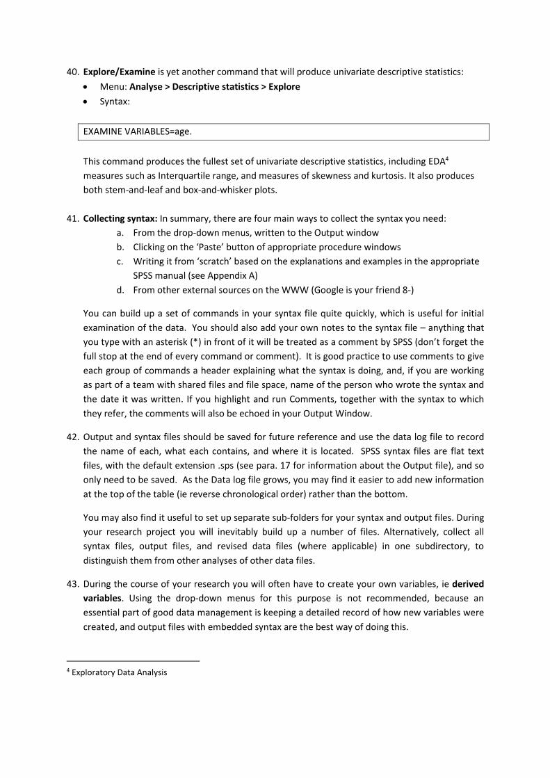
A number of output measures are available. For this exercise, make sure that Mean, Std

deviation, Range, Minimum and Maximum are selected, click ‘Continue’, and ‘OK’ when you are

returned to the previous dialogue screen.

The equivalent using syntax is:

DESCRIPTIVES VARIABLES=hospnum rdelay age / STATISTICS=MEAN STDDEV RANGE MIN MAX.

EXECUTE.

The Output window should now list the scale variables selected, showing their count (‘N’, minimum, maximum, range, mean and standard deviation (spread around the mean), as well as the SPSS commands that generated the output.

Notice the difference in the statistics provided by the Frequencies versus the Descriptives

procedures for the variable AGE.

What is the mean of the AGE variable? Can you get this from Frequencies or Descriptives? What is the median of the AGE variable? Can you get this from Frequencies or Descriptives? What is the mode of the AGE variable? Can you get this from Frequencies or Descriptives? What is the standard deviation of the AGE variable? Can you get this from Frequencies or Descriptives?

40. Explore/Examine is yet another command that will produce univariate descriptive statistics:

Menu: Analyse > Descriptive statistics > Explore

Syntax:

EXAMINE VARIABLES=age.

This command produces the fullest set of univariate descriptive statistics, including EDA4

measures such as Interquartile range, and measures of skewness and kurtosis. It also produces

both stem-and-leaf and box-and-whisker plots.

41. Collecting syntax: In summary, there are four main ways to collect the syntax you need:

a. From the drop-down menus, written to the Output window

b. Clicking on the ‘Paste’ button of appropriate procedure windows

c. Writing it from ‘scratch’ based on the explanations and examples in the appropriate

SPSS manual (see Appendix A)

d. From other external sources on the WWW (Google is your friend 8-)

You can build up a set of commands in your syntax file quite quickly, which is useful for initial

examination of the data. You should also add your own notes to the syntax file – anything that

you type with an asterisk (*) in front of it will be treated as a comment by SPSS (don’t forget the

full stop at the end of every command or comment). It is good practice to use comments to give

each group of commands a header explaining what the syntax is doing, and, if you are working

as part of a team with shared files and file space, name of the person who wrote the syntax and

the date it was written. If you highlight and run Comments, together with the syntax to which

they refer, the comments will also be echoed in your Output Window.

42. Output and syntax files should be saved for future reference and use the data log file to record

the name of each, what each contains, and where it is located. SPSS syntax files are flat text

files, with the default extension .sps (see para. 17 for information about the Output file), and so

only need to be saved. As the Data log file grows, you may find it easier to add new information

at the top of the table (ie reverse chronological order) rather than the bottom.

You may also find it useful to set up separate sub-folders for your syntax and output files. During

your research project you will inevitably build up a number of files. Alternatively, collect all

syntax files, output files, and revised data files (where applicable) in one subdirectory, to

distinguish them from other analyses of other data files.

43. During the course of your research you will often have to create your own variables, ie derived

variables. Using the drop-down menus for this purpose is not recommended, because an

essential part of good data management is keeping a detailed record of how new variables were

created, and output files with embedded syntax are the best way of doing this.

4 Exploratory Data Analysis

However, if you find that you still prefer to use drop-down menus, you should make sure to

always either paste what you have done into a syntax file and/or save the output file with the

applicable commands in it.