Data Mining and Visualization of the Alabama Accident Database

By

Michael Conerly, Brian Gray, Kevin Busby and Edward Mansfield Department of Management Science and Statistics

University of Alabama Tuscaloosa, Alabama

Prepared by

UTCA University Transportation Center for Alabama

The University of Alabama, The University of Alabama at Birmingham, and The University of Alabama in Huntsville

UTCA Project Number 99113 August, 2000

Technical Report Documentation Page 1. Report No FHWA/CA/OR-

2. Government Accession No. 3. Recipient Catalog No.

5. Report Date August 2000

4. Title and Subtitle Data Mining and Visualization of the Alabama Accident Database

6. Performing Organization Code

7. Authors Michael Conerly, Brian Gray, Kevin Busby and Edward Mansfield

8. Performing Organization Report No.

10. Work Unit No.

9. Performing Organization Name and Address Dept of Management Science and Statistics University of Alabama Box 870226 Tuscaloosa, Alabama 35487-0226

11. Contract or Grant No. DRTS98-G-0028

13. Type of Report and Period Covered Final Report/ 8/15/99 – 8/15/00

12. Sponsoring Agency Name and Address The University Transportation Center for Alabama Box 870205, 275 HM Comer Mineral Industries Bldg. Tuscaloosa, AL 35487-0205

14. Sponsoring Agency Code

15. Supplementary Notes 16. Abstract The Alabama Department of Public Safety has developed and maintains a centralized database that contains traffic accident data collected from crash reports completed by local police officers and state troopers. The Critical Analysis Reporting Environment (CARE), developed by Dr. David Brown and the Computer Science Department of the University of Alabama, provides web-based access to this database along with some basic statistical summary capabilities. In our research project, we employed existing multivariate data exploration tools to explore these databases for interesting and useful information that might lead to improved highway safety. Our analysis of the data led to the discovery of numerous data entry and variable definition problems in the Alabama Accident Databases. In this report, we describe these problems and make recommendations for the improvement of future data collection and the CARE system. Ultimately, these data quality issues lead us to conclude that meaningful statistical modeling of the existing data for the prediction of injuries and fatalities in traffic accidents is not feasible until these problems are corrected. 17. Key Words Education, Safety, Accident Analysis, Graphics, Statistics.

18. Distribution Statement

19. Security Classif (of this report) Unclassified

20. Security Classif. (of this page) Unclassified

21. No of Pages 28

22. Price

Form DOT F 1700.7 (8-72)

Contents

Contents………………………………………………………………………………….. iii List of Tables…………………………………………………………………………….. iv List of Figures …………………………………………………………………………… iv Executive Summary…...….……………………………………………………………… v

1.0 Overview …….…………………………………………………………………...…. 1 1.1 Introduction …………………………………………….……………………...… 1 1.2 Problem Statement ……………………………………..………………………… 1 1.3 Overall Project Approach……………………………….………………………... 2

2.0 Background…………………………………………………………………………... 3 3.0 Methodology ………………………………………………………………………… 4 3.1 Data Import and Cleaning…..………………………….………………………… 4 3.2 Problem Statement ……………………………………..………………………… 4 3.2.1 Logistic Regression..…………………………….………………………… 4 3.2.3 Classification and Regression Trees…………….………………………… 5 3.2.2 Mosaic Plots……………………………………..………………………… 5

4.0 Project Findings and Results………………………………………………………… 6 4.1 CARE Issues……………..………………………….……………………………. 6 4.2 Variable Coding/Definition Errors……………………..………………………… 6 4.3 Exploratory Data Analysis..…………………………….………………………… 9 4.3.1 One-, Two- and Three-Way Frequency Tables…..………………………… 9 4.3.2 Logistic Regression…………………………..…..………………………… 9 4.3.3 Classification and Regression Trees……………..………………………… 10 4.3.4 Mosaic Plots……………………….……………..………………………… 14 5.0 Project Conclusions and Recommendations ………………………………………… 16 5.1 Data Collection and Coding...………………………….………………………… 16 5.2 CARE…………………………………………………..………………………… 17 5.3 Statistical Models Limited by Data Quality Problems.….………………..……… 17 6.0 References …………………………………………………………………………… 18 Appendix A: Variable Names in the Accident Databases…………………………..…… 19 Appendix B: Variable Names in the Occupant Databases…………………………..…… 22

iii

List of Tables

Number Page 4-1 Cross tabulation of ACCIDENT_SEVERITY and

HIGHEST_OCCUPANT_SEVERITY……………………………………… 7

4-2 Partial cross tabulation of CAUSAL_VEHICLE_TYPE and

TYPE_VEHICLE_C………………………………………………………… 8

4-3 Code values for RESTRAINT_USED_DRIVER_C………………………… 8

List of Figures

Number Page 4-1 S-Plus report for CART model………………….…………………………… 11 4-2 S-Plus CART tree…………………………………….……………………… 12 4-3 Enhanced CART tree combining information from Figures 4-1 and 4-2...…… 13 4-4 Mosaic plot displaying CART model from Figure 4-1..……………………… 14

iv

Executive Summary The Alabama Department of Public Safety has developed and maintains a centralized database that contains traffic accident data collected from crash reports completed by local police officers and state troopers. The Critical Analysis Reporting Environment (CARE), developed by Dr. David Brown and the Computer Science Department of the University of Alabama, provides web-based access to this database along with some basic statistical summary capabilities, primarily one- and two-variable frequency distributions and bar charts. In our research project, we employed existing multivariate data exploration tools (including logistic regression, classification and regression trees (CART), and mosaic plots) that go beyond CARE’s capabilities to search these databases for interesting relationships that might not be found by considering only one and two variables at a time. Our ultimate goal was to find useful information that might lead to improved highway safety. In particular, we hoped to identify important determinants of injuries and fatalities in traffic accidents. Our analysis of the data led to the discovery of numerous data entry errors and variable definition problems in the Alabama Accident Databases. Ultimately, these data quality issues led us to conclude that meaningful statistical modeling of the existing data for the prediction of injuries and fatalities in traffic accidents is not feasible. In this report, we describe these problems and make recommendations for the improvement of future data collection and the CARE system.

v

1. Overview 1.1 Introduction The Alabama Department of Public Safety has developed and maintains a centralized database that contains accident data collected from crash reports completed by local police officers and members of the Alabama Highway Patrol. Data gathered from each accident are recorded in two databases: the Accident Database and the Occupant Database. The CARE (Critical Analysis Reporting Environment) system, maintained by Dr. David Brown and the Computer Science Department at the University of Alabama, allows access to the databases with basic statistical analysis capabilities for categorical data (such as one-variable frequency distributions, bar charts, and two-variable frequency tables). Analysis of these data sets could potentially yield useful information for improving traffic safety in the state of Alabama. 1.2 Problem Statement The CARE system allows for frequency distributions, bar charts and two-way frequency tables of the data. IMPACT (Information Mining Performance Attainment Control Technique), a component of CARE, “performs true automated information discovery by systematically finding all overrepresentations between any two subsets.” An IMPACT analysis essentially considers the relationship between two variables in the form of two-way conditional frequency tables. As such, IMPACT is unable to detect more complicated relationships or interactions among the factors that lead to an accident. For example, the combination of lack of seat belt use, alcohol consumption, and rainy conditions may result in accident severity greater than that indicated by the sum of the individual effects. In this study, we attempted to explore these multivariate relationships to better understand the factors leading to serious accidents. In the course of our analysis, we discovered several quality issues within the Alabama Highway Accident Database that eventually became a major obstacle in our analysis of the data. Details of these problems and their impact are given later in this report along with recommendations for the improvement of data collection in the future.

1

1.3 Overall Project Approach

We performed statistical analyses of the Alabama Accident Databases that go beyond those currently employed in the CARE system, including:

• multivariate data displays (mosaic plots, three- and higher-way frequency tables, etc.) • multivariate data modeling (logistic regression, CART analysis, etc.) • multivariate outlier detection

The modeling of multivariate relationships among the variables in the Alabama traffic accident database is important for two reasons. First, statistical models help us to better understand the relationships among several variables at a time by summarizing the overall, or average, behavior. Secondly, once the average behavior is determined, it becomes easier to identify the outliers or unusual data that are not predicted well by the models. These outliers are typically indications of recording errors, but they often provide useful information about important variables left out of the analysis or identify a segment of the data that is quite unlike the rest of the data. The modeling techniques were used to build mathematical models of relationships among variables. These methods are distinguished by the types of variables that they can analyze. The two major classifications of variables are categorical and quantitative. Categorical variables, such as county and condition of roadway, classify observations into groups or categories. Quantitative variables, such as age of driver and blood alcohol level, are numerical measurements made on observations. Regression analysis deals primarily with relationships among quantitative variables, while log-linear models deal primarily with associations in categorical data. Classification and regression tree (CART) analysis is suitable for modeling and exploring relationships among quantitative and categorical variables. Complicated relationships can be difficult to identify even in small data sets. Larger databases, such as the Alabama Accident Databases, present additional problems for analysis. The general area for exploring massive data sets is referred to as data mining. The field of data mining overlaps many disciplines, primarily statistics, computer science, and information systems. Data storage and retrieval is generally considered to be an information systems issue. Algorithms useful for extracting information from databases are of particular interest in computer science. Statistics is a discipline that studies the best ways to analyze the data and seek meaningful relationships among sets of variables. Existing data mining techniques are useful for computer-assisted sifting through the complexities interwoven among large numbers of variables. As stated earlier, in data analysis we are concerned with identifying typical behavior (patterns and relationships) and atypical behavior (outliers) in data. Outliers are sometimes the most important observations in a data set because they can provide information about relationships between variables not contained in the regular data. We detected such data through the use of frequency tables, logistic regression and influence diagnostics (computed after the model fitting described above). In most cases, these outliers indicated data recording issues that need to be addressed. We provide some examples of these problems and recommendations in this report.

2

2. Background The Alabama Accident Databases contains data obtained from the crash report forms completed by state troopers or local police officers at traffic accident scenes. These data from the crash report form are entered into the database by the Alabama Department of Public Safety. Currently there are two distinct databases available in CARE, the Accident and Occupant Databases, for each of the years from 1994 to 1998. The 1998 Accident Database contains more than 200 variables measured on 138,000 accidents. These data specify the nature of the accident, any contributing factors, types of vehicles involved, accident severity, etc. (See Appendix A for a listing of variables in the accident database.) The 1998 Occupant Database consists of 18 variables (such as seating position, restraint used, etc.) measured for more than 379,000 occupants of vehicles involved in the 138,000 accidents. (See Appendix B for a listing of variables in the Occupant Database.) Led by Dr. David Brown, a group of faculty members and students in the University of Alabama Computer Science Department developed a national award winning computer system that can be used to analyze the Alabama Accident Database as well as several other state and federal traffic databases. The program, called Critical Analysis Reporting Environment (CARE), allows the user to use conditioning statements to create subsets of the large database that meet the criteria specified by the user. For example, the user might request all alcohol-related incidents involving drivers under 19 years of age. Summaries of the identified subset of the database are then presented to the user in numerical, tabular (frequency distributions and cross-tabulations), or graphical form (bar charts). CARE also includes an Information Mining Performance Attainment Control Technique (IMPACT) module, which performs data mining involving two categorical variables at a time. This module systematically finds all “overrepresentations” between any two subsets of the data. For example, a comparison of weather-related accidents with nonweather-related accidents by county will tell which counties have higher than expected (as well as those with lower than expected) levels of weather-related accidents, so that countermeasures can begin to be considered in the most critical areas. The CARE system can be accessed at http://care.cs.ua.edu. It is available in both on-line and downloadable versions. Past studies utilizing the CARE system can also be found at this website.

3

3. Methodology 3.1 Data Import and Cleaning The main purpose of our project was to consider statistical analyses of the accident data that go beyond CARE’s statistical capabilities. This necessitated exporting the data from CARE to the SAS and S-Plus environments for additional analyses as described in the next section. The CARE system allows exporting of the accident databases via a tool called DataGen. This module exports a database into a large ASCII text file. We read this text file into SAS Version 8.0 because of its ability to manage large data files. A large number of errors are to be expected with any massive data set. Our first step in the process of resolving the errors was to compare frequency distributions between SAS and CARE for each variable to detect unusual values and any inconsistencies. After resolving these data problems, our next step was to consider two- and three-way frequency tables of related variables to uncover additional miscodings and inconsistencies. A list of problems detected during this phase of the study is given in the Project Findings and Results Section. 3.2 Statistical Methods Nearly all of the data variables contained in the accident databases are categorical in nature. Several of the variables are discrete versions of numeric variables such as age, blood alcohol level, etc. The nature of these data severely limits the array of statistical methods that are applicable for analyzing the accident database. Additionally, effective graphical displays for multivariate categorical data are practically nonexistent. 3.2.1 Logistic Regression Regression analysis is used to predict or estimate the value of a response variable based on the values of several predictor variables. Generally there is a single response variable of interest that depends on a number of related quantities. Regression procedures are among the most widely used of statistical techniques but are intended for quantitative response variables. For categorical responses, logistic regression provides an alternative method. Typically, logistic regression models are used to predict the probability of a certain event. The data used to develop such models are based on binary response variables where, for each observation, the response variable is recorded as “1” or “0” denoting that the event of interest did occur or did not occur, respectively. In the current study, we used logistic regression to estimate the probability that an

4

accident results in injuries or fatalities. The predictor variables considered include the speed of vehicle, alcohol or drug use by the driver, and use of safety restraint devices. 3.2.2 Classification and Regression Trees The classification and regression trees (CART) methodology is a relatively new approach to the problem of predicting a response variable on the basis of several predictor variables. Typically, the response variable is categorical, so that the problem reduces to one of classification based on auxiliary information. Predictors can be either categorical or quantitative. At the beginning of the CART algorithm, all of the observations are contained in the root node of what will eventually become a binary tree structure. The observations in the root node are split into two child nodes based on the values of a predictor variable. The predictor variable and splitting rule are chosen to make the observations within each node as homogeneous as possible with respect to the response variable. The splitting process continues with the child nodes. The process stops when the homogeneity within terminal nodes in the tree cannot be improved with further splits. The tree can be used to (1) classify (or predict) new observations and (2) estimate conditional probabilities of response categories based on the values of the predictor variables. One advantage of CART models is their ability to handle either categorical or quantitative variables and to more easily model complicated interactions than logistic regression models. For the current research project, we used CART to estimate the probability of injuries and/or fatalities in traffic accidents given predictor variable information. 3.2.3 Mosaic Plots The Alabama Accident Database contains over 200 variables, most of which are categorical in nature. To display categorical data, one typically uses frequency tables or multi-way tables that exhibit the number of observations falling into each distinct category or combination of categories. There are limited techniques available for displaying these data in a chart or graph. Michael Friendly (1994, 1999) recently described the use of mosaic plots for displaying multi-way tables. These plots are a visual display of the counts in multi-way tables. These plots can be color- or symbol-coded to denote cells that have more or fewer observations than expected under the assumption of independence among the variables. We downloaded SAS code from Michael Friendly’s website (http://www.math.yorku.ca/SCS/friendly.html#grmodel) to construct mosaic plots for the Alabama Accident data.

5

4. Project Findings and Results 4.1 CARE Issues In order to proceed with a multivariate analysis of the databases, it was necessary to export the data from CARE into ASCII text files which could then be read into SAS, S-Plus, and other software packages. DataGen is the CARE component responsible for exporting data from the accident databases. Initially, DataGen was not exporting all of the data. After conferring with Dr. Brown and his staff, this problem was resolved in a timely manner. However, on the next attempt to export the data, we discovered that values of some variables were missing at random. The fields read subsequent to the missing values were recorded in the wrong columns resulting in misalignments in the data set. Dr. Brown’s staff was helpful in resolving these problems, which led to further modifications of DataGen. In the process of comparing frequency distributions produced by SAS and CARE, we discovered many instances of values outside the defined range for a variable that were reported by SAS but not by CARE. Some variables defined in the accident databases do not have a missing value code, so data entry personnel enter values outside the valid range to indicate missing or unknown values. But, values outside the valid range might also indicate data entry errors. In either event, CARE does not include these in its frequency tables. This omission inflates the percentages of accidents in all of the valid categories. Because of the nature of the data and the size of the data set, numerous coding errors such as these are to be expected and are not ignorable, especially if the pattern of missing data values is nonrandom. We also discovered that CARE omits values of zero in its frequency tables for some variables, such as NUMBER_INJURED, where zero is a valid response. This results in unintentional conditioning of the reported percentages. For example, CARE reports that 78% of one-car accidents have exactly one injury when in fact the actual value is 27%. CARE's calculation considers only those accidents involving at least one injury. Since most accidents do not result in injuries, CARE’s statistics are computed after ignoring the bulk of the data. 4.2 Variable Coding/Definition Errors In the course of our analysis of the data, we discovered many variable coding/definition errors. Among these were the following:

• Inconsistent codings between variables. Some variables in the database have codes for “missing”, “not applicable”, “unknown”, etc., but many do not. We are uncertain as to the difference in meaning between “missing” and “unknown,” although some variables

6

have both as possible codes. For those variables without a missing code, it appears that data entry personnel often use a value outside the valid range to indicate a missing value. For those variables that do have missing codes, these code values differ from one variable to another.

• Poor definition of variable levels. Certain levels of variables are difficult to interpret.

For example, an “airbag inoperable” data value for RESTRAINT_USED_DRIVER_C is unclear. Given that 14% of all 1998 accidents have this code, we are led to believe that “inoperable” does not simply mean “defective”. “Airbag inoperable” could mean that the airbag was defective, that it did not deploy, or that it was not replaced after previous deployment. As another example, TEST_RESULTS_DRIVER_C has a code for “none.” This could be interpreted as zero alcohol level, a test was not given, the test was refused, or the data is missing. It appears that each of these interpretations was applied in coding data.

• Inconsistencies among variables. In some instances where variables containing similar

information should agree, they do not. For example, ACCIDENT_SEVERITY might indicate an injury in an accident, yet HIGHEST_OCCUPANT_SEVERITY indicates that no injury occurred in the accident. Table 4-1 below highlights this and other inconsistencies for these two variables. The five shaded cells should contain zeros by definition, yet do not indicating 5,272 misclassified accidents.

Table 4-1. Cross Tabulation of ACCIDENT_SEVERITY and HIGHEST_OCCUPANT_SEVERITY

Highest Occupant Severity

Killed Injury1 Injury2 Injury3 No Injury Total

Accident Property Damage 0 0 0 0 104375 104375 Severity Injury 0 15286 3754 8109 5028 32177

Fatality 712 142 14 7 81 956

Total 712 15428 3768 8116 109484 137508

By examining a three-way frequency table of HIGHEST_OCCUPANT_SEVERITY, NUMBER_INJURED, and ACCIDENT_SEVERITY, we determined that the HIGHEST_OCCUPANT_SEVERITY variable is the one most likely in error. This is unfortunate because HIGHEST_OCCUPANT_SEVERITY provides a finer breakdown of the degree of injury than ACCIDENT_SEVERITY and would have been a better choice as a response variable. As another example, CAUSAL_VEHICLE_TYPE does not agree with TYPE_VEHICLE_C in all cases. These two variables have exactly the same set of possible variable values, yet are not in agreement for a large number of accidents. Table 4-2 below shows a 4 × 4

7

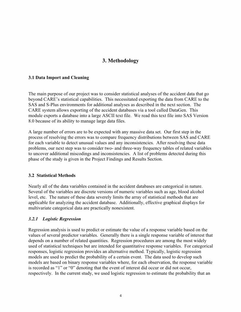
subtable of the cross-tabulation of CAUSAL_VEHICLE_TYPE and TYPE_VEHICLE_C corresponding to the values “automobile”, “station wagon”, “pickup truck”, and “van”. The 1,667 observations in the shaded off-diagonal cells in the table are misclassified vehicle types, i.e., the values recorded for the two variables are different when they should be identical.

Table 4-2. Partial Cross Tabulation of CAUSAL_VEHICLE_TYPE and TYPE_VEHICLE_C

Type Vehicle C

Auto Station Wagon

Pickup Van

Causal Auto 83545 59 560 141 Vehicle Station Wagon 32 1517 12 3

Type Pickup 570 14 34113 67 Van 153 5 51 6745

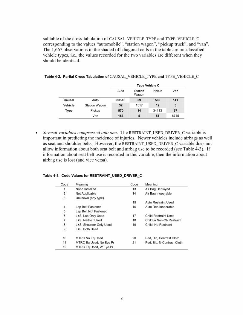
• Several variables compressed into one. The RESTRAINT_USED_DRIVER_C variable is important in predicting the incidence of injuries. Newer vehicles include airbags as well as seat and shoulder belts. However, the RESTRAINT_USED_DRIVER_C variable does not allow information about both seat belt and airbag use to be recorded (see Table 4-3). If information about seat belt use is recorded in this variable, then the information about airbag use is lost (and vice versa).

Table 4-3. Code Values for RESTRAINT_USED_DRIVER_C

Code Meaning Code Meaning

1 None Installed 13 Air Bag Deployed 2 Not Applicable 14 Air Bag Inoperable 3 Unknown (any type) 15 Auto Restraint Used

4 Lap Belt Fastened 16 Auto Res Inoperable 5 Lap Belt Not Fastened 6 L+S, Lap Only Used 17 Child Restraint Used 7 L+S, Neither Used 18 Child in Non-Ch Restraint 8 L+S, Shoulder Only Used 19 Child, No Restraint 9 L+S, Both Used

10 MTRC No Eq Used 20 Ped, Bic, Contrast Cloth 11 MTRC Eq Used, No Eye Pr 21 Ped, Bic, N-Contrast Cloth 12 MTRC Eq Used, W Eye Pr

8

• Implausible events. Certain combinations of variables yield circumstances, which should not occur. For example, there are 656 out of 28,048 one-car accidents in 1998 with no pedestrians and no driver in the causal vehicle. As another example, 256 drivers in the 1998 accident database are under the age of 14. Of those 256, 18 are listed as being one year old.

While any one of the problems discussed in this section might seem minor in terms of the percentage of accident records affected, their combined effect extends to well more than half of the database records. 4.3 Exploratory Data Analysis In the first year of our proposed two-year project, the primary goal was exploration of the data to gain initial insights into relationships among the variables and to determine which statistical techniques might be best suited to modeling the data. In addition, this exploration identified the database problems discussed in sections 4.1 and 4.2. 4.3.1 One-, Two- and Three-way Frequency Tables Initially, we used one-way tables to compare the frequency distributions of SAS and CARE. This led to the discovery that missing values are not consistently coded across different variables in the accident database. In some instances, there is not a missing value code while for other variables, there are multiple codes used for missing values (missing, unknown, 0, undefined codes, etc.). “Undefined codes” means that when a data value was missing, the person entering the data would use any value outside the range defined by CARE for the variable. We also used multi-way tables to identify conflicts among similar variables as illustrated in Table 4-1. For analysis purposes, we used two- and three-way tables to identify predictor variables that were related to our response variable, NUMBER_INJURED. Subsequently, these identified variables were candidates for inclusion in stepwise logistic regression modeling. 4.3.2 Logistic Regression Multi-way tables are limited by the number of variables that can be considered simultaneously. Logistic regression provides a means for modeling a categorical response variable as a function of several predictor variables. Initial analysis with logistic regression suggested the presence of high-order interaction effects. Because of the large number of predictor variables, even the first-order models we considered were cumbersome. Inclusion of second- and higher-way interactions would have led to unwieldy models (especially for categorical variables, each of which has to be recoded as multiple indicator variables). This led us to consider classification and regression tree (CART) analysis. Significant variables found in first-order logistic regression models were carried over to our CART analyses.

9

4.3.3 Classification and Regression Trees (CART) The Classification and Regression Trees (CART) methodology is a relatively new addition to the collection of statistical tools for modeling data (see Breiman, et al (1984)). Typically, the value of a categorical response variable is modeled or predicted on the basis of the values of several categorical and quantitative explanatory variables. (CART has also been extended to handle quantitative response variables.) One major advantage of CART over logistic regression is its ability to automatically detect and model high-order interactions among the predictor variables. CART also has the ability to handle missing explanatory variable data by treating the missing value as just another level of the explanatory variable. (If the missing variable turns out to be important in the model, it is an indication that the “missingness” is not at random, but related to some other variables, possibly not in the data set.) Suppose that the response is binary (i.e., only two possible outcomes). At the beginning of the CART algorithm, all observations are grouped into a single node. Each predictor variable is considered in turn to find the “best split” of the initial node into two subsets, a “left child” node and a “right child” node. A split is determined by the choice of a single predictor variable and a partitioning of its possible values into two sets. All observations with values of the predictor variable in the first set go to the left child node and the remaining observations go to the right child node. The “best split” is the one that makes the observations within each node as similar as possible and between the two nodes as dissimilar as possible with respect to the response variable. The splitting process is repeated for each resulting child node until all terminal nodes in the tree are as “pure” as possible. We considered a number of different CART models, which provided us with several insights about the data set. A simple S-Plus example of a CART analysis, involving the prediction of the binary variable INJURIES (0 = no injury/fatality, 1 = at least 1 injury/fatality) as a function of OFCR_OPINION_SOBRIETY (VAR_115) and DL_STATUS_DRIVER_C (var_61), is shown in Figures 4-1 and 4-2.

10

*** Tree Model *** Classification tree: tree(formula = injuries ~ VAR.115 + var.61, data = onecar.98, na.action = na.exclude, mincut = 500, minsize = 1000, mindev = 0.01) Number of terminal nodes: 8 Residual mean deviance: 1.245 = 34910 / 28040 Misclassification error rate: 0.338 = 9480 / 28048 node), split, n, deviance, yval, (yprob) * denotes terminal node 1) root 28048 36120.0 NoInjs ( 0.3443 0.6557 ) 2) VAR.115:-99,1,3 23883 29860.0 NoInjs ( 0.3177 0.6823 ) 4) var.61:Invalid 968 1339.0 NoInjs ( 0.4731 0.5269 ) * 5) var.61:Current,Missing,N/A 22915 28410.0 NoInjs ( 0.3111 0.6889 ) 10) VAR.115:1 20559 25320.0 NoInjs ( 0.3058 0.6942 ) 20) var.61:Current,Missing 19828 24210.0 NoInjs ( 0.2995 0.7005 ) * 21) var.61:N/A 731 1012.0 NoInjs ( 0.4774 0.5226 ) * 11) VAR.115:-99,3 2356 3072.0 NoInjs ( 0.3574 0.6426 ) 22) var.61:Current,Missing 1313 1810.0 Injs ( 0.5446 0.4554 ) * 23) var.61:N/A 1043 772.7 NoInjs ( 0.1218 0.8782 ) * 3) VAR.115:2,4 4165 5774.0 NoInjs ( 0.4968 0.5032 ) 6) var.61:Invalid,Missing 1003 1387.0 Injs ( 0.5294 0.4706 ) * 7) var.61:Current,N/A 3162 4381.0 NoInjs ( 0.4864 0.5136 ) 14) var.61:Current 2568 3559.0 NoInjs ( 0.4926 0.5074 ) * 15) var.61:N/A 594 819.6 NoInjs ( 0.4596 0.5404 ) *

Figure 4-1. S-Plus Report for CART Model. Figure 4-1 details the splitting process of the CART analysis. At the root node, which contains all 28,048 one-car, no pedestrian accidents in 1998, 34.43% of accidents resulted in at least one injury. In the first split, OFCR_OPINION_SOBRIETY (VAR_115) is determined to be the best splitting variable with the 23,883 accidents having values of “none”, “drugs”, or “missing” going to the left child node and the remaining 4,165 accidents having values of “alcohol” or “drugs and alcohol” going to the right child node. Of those 23,883 accidents in the left node, 31.77% resulted in at least one injury. Of the 4,165 accidents in the right node, 49.68% resulted in at least one injury. From this we would conclude that the unconditional probability of injury in a one-car accident is about 35%, but that the conditional probability of an injury in an accident given that the driver was using either alcohol or alcohol and drugs is nearly 50%. Clearly, the information contained in OFCR_OPINION_SOBRIETY (VAR_115) is useful in assessing the risk of injury. The splitting process continues with the child nodes and stops when further splitting fails to yield improvements. Figure 4-1 shows the results of the splitting process by node. For example, in Node 6 of the report, which corresponds to the 1,003 accidents involving 1) alcohol or a combination of drugs and alcohol and 2) invalid or missing driver licenses, 52.94% of the accidents resulted in at least one injury.

11

|VAR.115:abd

var.61:b

VAR.115:bvar.61:ac var.61:ac

var.61:bc var.61:a

NoInjs

NoInjs NoInjs

Injs NoInjs

Injs NoInjs NoInjs

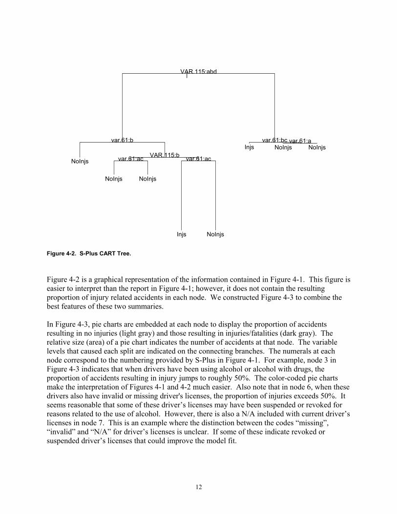
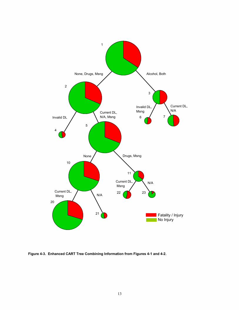
Figure 4-2. S-Plus CART Tree. Figure 4-2 is a graphical representation of the information contained in Figure 4-1. This figure is easier to interpret than the report in Figure 4-1; however, it does not contain the resulting proportion of injury related accidents in each node. We constructed Figure 4-3 to combine the best features of these two summaries. In Figure 4-3, pie charts are embedded at each node to display the proportion of accidents resulting in no injuries (light gray) and those resulting in injuries/fatalities (dark gray). The relative size (area) of a pie chart indicates the number of accidents at that node. The variable levels that caused each split are indicated on the connecting branches. The numerals at each node correspond to the numbering provided by S-Plus in Figure 4-1. For example, node 3 in Figure 4-3 indicates that when drivers have been using alcohol or alcohol with drugs, the proportion of accidents resulting in injury jumps to roughly 50%. The color-coded pie charts make the interpretation of Figures 4-1 and 4-2 much easier. Also note that in node 6, when these drivers also have invalid or missing driver's licenses, the proportion of injuries exceeds 50%. It seems reasonable that some of these driver’s licenses may have been suspended or revoked for reasons related to the use of alcohol. However, there is also a N/A included with current driver’s licenses in node 7. This is an example where the distinction between the codes “missing”, “invalid” and “N/A” for driver’s licenses is unclear. If some of these indicate revoked or suspended driver’s licenses that could improve the model fit.

12

1

2

4

5

10

20

21

11

22

23

3

6

7

None, Drugs, Msng Alcohol, Both

Invalid DLCurrent DL,N/A, Msng

Invalid DL,Msng

Current DL,N/A

Drugs, MsngNone

Current DL, Msng N/A

Current DL, Msng

N/A

Fatality / Injury No Injury

Figure 4-3. Enhanced CART Tree Combining Information from Figures 4-1 and 4-2.

13

4.3.4 Mosaic Plots Mosaic plots are convenient tools for graphically displaying categorical data. After generating different CART models, we used mosaic plots as another means of displaying results from our exploratory analysis. These are useful graphical tools for two, three or possibly four categorical variables with few levels each; however, for many variables and/or levels, these plots become very difficult to interpret. The size of the blocks is related to the number of accidents occurring at that specific combination of variables. These plots can be used to decipher conditional, joint, or mutual independence among the variables.

Alabama Highway Accident Data

++

- -

- -

++

++ ++ ++++

- - -

-+-++

++

––

– - - –++ ++ ++

++- -

- -

-+

- -

Missing None Alcohol Drugs Both

Injury/Fatality

No Injury/Fatality

Figure 4-4. Mosaic Plot Displaying CART Model from Figure 4-1. Figure 4.4 is a mosaic plot display for a three-way frequency table of INJURIES, OFCR_OPINION_SOBRIETY_C and DL_STATUS_DRIVER_C. From bottom to top, the “rows” indicate missing, current, invalid, and N/A, with regard to the driver’s license of the driver of the causal vehicle. From left to right, the “columns” represent missing, none, alcohol, drugs, and both alcohol and drugs for the officer's opinion of the sobriety of the driver of the causal vehicle. The horizontal splits within each of the cells delineated by the rows and columns indicate injury

14

(bottom) or no injury (top). Ignoring these horizontal splits, the total area associated with a block or cell is proportional to the number of accidents in that cell. The area below the horizontal split in a block is proportional to the conditional probability of injury given the values of sobriety level and driver’s license status defining that cell. The symbol shown within a cell indicates how much the observed number of accidents in the cells differs from the expected number under an assumption of joint independence among the three variables. The joint independence assumption implies that the three variables are unrelated. The symbol “–” (“– –”) indicates that the observed count is low (extremely low) compared to the expected count. The symbol “+” (“++”) indicates that the observed count is high (extremely high) compared to the expected count. The pattern of symbols within cells of the mosaic plot provides clues as to the relationships among the variables. The probability of injury is lowest for drivers in one-car accidents that have a current driver’s license and appear to be sober. The use of alcohol, drugs or both increases the probability of injury fairly dramatically for the current driver’s license group. The block corresponding to current driver’s license and missing sobriety seems to behave more like the nonsober groups. It would be interesting to know what leads to missing values in this situation. Similarly, the block corresponding to N/A driver’s license and missing sobriety has a suspiciously low probability of injury suggesting that the data are not missing at random.

15

5. Project Conclusions and Recommendations Given the problems we encountered with the accident database, most of our recommendations focus on improvements to the data collection process and suggestions for improvements to the CARE system. 5.1 Data Collection and Coding The following is a list of items that would enhance the quality of the accident database. Many of these items have been mentioned in earlier sections of this report.

• Determine the sources of data quality problems in data collection and data entry and attempt to eliminate these problems. Improve the accident form to facilitate data collection, i.e., to improve accuracy and completeness in data recording, and to eliminate data recording errors at the accident scene. Identify the sources of common coding errors occurring in data entry at the Department of Public Safety. Further study is needed in this area to develop specific recommendations.

• Eliminate redundant and/or error-prone coding in the accident and occupant databases by determining which variables are base variables and which variables are derived from the base variables. Data are entered for the base variables. Values of the derived variables are computed from these base fields.

• Create a concise data dictionary with clear definitions of variables and their levels. Make clear distinctions among not applicable (N/A), missing, unknown and zero values and include these where required.

• Clarify the safety equipment used by creating SEATBELT and AIRBAG variables to replace the RESTRAINT_USED_DRIVER_C variable in the accident databases and the SAFETY_EQUIPMENT variable in the occupant databases.

• Work toward the use of on-site, electronic data entry with automatic consistency checks to eliminate transcription errors. Driver information could be encoded in a magnetic strip on the driver’s license and scanned at the scene of the accident. Similarly, the vehicle identification number (VIN) and/or the license plate number could be scanned or entered to access an electronic database that would provide complete information about an accident vehicle.

16

5.2 CARE The following are suggestions for improvements to CARE:

• Include zero levels, missing codes and other aberrant codes in all frequency distributions to eliminate unintentional conditioning and to identify coding errors in the data.

• Provide three- and higher-way tables of frequency distributions to describe higher-order interactions.

• Improve DataGen's exporting speed and its ability to handle missing data. 5.3 Statistical Models Limited by Data Quality Problems Our original proposal called for limited statistical modeling of the accident data. In our preliminary exploration of the data, it became clear that data quality problems described in sections 4.1 and 4.2 limit any efforts to adequately model the data. One of the main inhibiting factors is the coding of the variables RESTRAINT_USED_DRIVER_C in the accident databases and SAFETY_EQUIPMENT in the occupant databases. As mentioned earlier, the coding of these variables confounds the effects of seatbelts and airbags, making it impossible to sort out their individual contributions. A priori, it is reasonable to assume that these variables are an important predictor of injury. This was borne out in our initial modeling attempts. In CART models we considered early in our analyses, RESTRAINT_USED_DRIVER_C was typically one of the first variables picked as a predictor of INJURIES. Splits based on this variable tended to divide the accidents into those in which a restraint of some type was used and those in which no restraints were used. Interestingly, the proportion of injuries in the “restraint used” nodes was higher than for the corresponding “no restraint used” nodes. While this seems contradictory, there are at least two possible explanations: (1) an airbag deploying when the driver is not wearing a seat belt could lead to an airbag-caused injury (but recall that we cannot identify these situations because of the way in which RESTRAINT_USED_DRIVER_C is defined). (2) Airbags tend to deploy only in relatively high-speed accidents, and injuries naturally tend to occur more often in high-speed accidents. In conclusion, we do not believe that it is possible to develop meaningful statistical models for predicting injuries and fatalities given the data quality problems encountered in the accident databases. In particular, the type and use of safety equipment is one of the most important variables to be considered in predicting injuries and fatalities. Because of the inherent problems in the coding of RESTRAINT_USED_DRIVER_C (and SAFETY_EQUIPMENT for occupants), including this variable in a model leads to bias and results that are suspect. On the other hand, not including this variable in a model biases the results given its importance (clearly a case of “damned if you do, damned if you don’t”).

17

6. References Friendly, Michael (1994), “Mosaic Displays for Multi-Way Contingency Tables,” Journal of the

American Statistical Association, 89, 190-200. Friendly, Michael (1994), “Extending Mosaic Displays: Marginal, Conditional and Partial Views

of Categorical Data, ” Journal of Computational and Graphical Statistics, 8, 373-395.

Hosmer, David W., Jr. and Lemeshow, Stanley (1989), Applied Logistic Regression, New York: Wiley.

Breiman, L., Friedman, J., Olshen, R. and Stone, C. (1984), Classification and Regression Trees, Belmont, CA: Wadsworth International.

18

Appendix A: Variable Names in Accident Database ACCIDENT_NUMBER ACCIDENT_SEVERITY ACTION_PEDESTRIAN AGE_OF_DRIVER_2 AGE_OF_DRIVER_3 AGE_OF_DRIVER_C AGE_PEDESTRIAN AIM_INTERSECTION_OR_SEGMENT AIM_MILESTONE_INDICATOR AMBULANCE_ARRIVAL_DELAY ATTACHMENT_VEHICLE_2 ATTACHMENT_VEHICLE_3 ATTACHMENT_VEHICLE_C BODY_STYLE_VEHICLE_2 BODY_STYLE_VEHICLE_3 BODY_STYLE_VEHICLE_C CASE_NUMBER CAUSAL_VEHICLE_CATEGORY CAUSAL_VEHICLE_TYPE CITATION_CHARGED_VEHICLE_2 CITATION_CHARGED_VEHICLE_3 CITATION_CHARGED_VEHICLE_C CITY CITY_INF CLOTHING_CONTRAST_PED CNTRBTING_ROAD_DEFECTS_VEH_2 CNTRBTING_ROAD_DEFECTS_VEH_3 CNTRBTING_ROAD_DEFECTS_VEH_C CONSTRUCTION_ZONE_UNIT_2 CONSTRUCTION_ZONE_UNIT_3 CONSTRUCTION_ZONE_UNIT_C CONTRIBUTING_DEFECT_VEHICLE_2 CONTRIBUTING_DEFECT_VEHICLE_3 CONTRIBUTING_DEFECT_VEHICLE_C CONTROL_ACCESS_HIGHWAY_LOCATION COUNTY COUNTY_I DAMAGE_SEVERITY_VEHICLE_2 DAMAGE_SEVERITY_VEHICLE_3 DAMAGE_SEVERITY_VEHICLE_C DAMAGE_VEHICLE_2 DAMAGE_VEHICLE_3 DAMAGE_VEHICLE_C DATE_OF_MONTH

DAY_OF_WEEK DIRECTION_OF_TRAVEL_VEH_2 DIRECTION_OF_TRAVEL_VEH_3 DIRECTION_OF_TRAVEL_VEH_C DISTANCE_TO_FIXED_OBJECT DL_RESTRICTION_STATUS_DRIVER_2 DL_RESTRICTION_STATUS_DRIVER_3 DL_RESTRICTION_STATUS_DRIVER_C DRIVER_CONDITION_DRIVER_2 DRIVER_CONDITION_DRIVER_3 DRIVER_CONDITION_DRIVER_C DRIVER_LICENSE_STATE_DRIVER_2 DRIVER_LICENSE_STATE_DRIVER_3 DRIVER_LICENSE_STATE_DRIVER_C DRIVER_LICENSE_STATUS_DRIVER_2 DRIVER_LICENSE_STATUS_DRIVER_3 DRIVER_LICENSE_STATUS_DRIVER_C DRIVER_LICENSE_TYPE_DRIVER_2 DRIVER_LICENSE_TYPE_DRIVER_3 DRIVER_LICENSE_TYPE_DRIVER_C EMS_TRANSPORT_PEDESTRIAN ESTIMATED_SPEED_VEHICLE_2 ESTIMATED_SPEED_VEHICLE_3 ESTIMATED_SPEED_VEHICLE_C EVENT_LOCATION EVENT_LOCATION_DRIVER_2 EVENT_LOCATION_DRIVER_3 EVENT_LOCATION_DRIVER_C EVENT_LOCATION_PEDESTRIAN FIRST_AID_BY_PEDESTRIAN FIRST_HARMFUL_EVENT HAZARDOUS_CARGO_VEHICLE_2 HAZARDOUS_CARGO_VEHICLE_3 HAZARDOUS_CARGO_VEHICLE_C HIGHEST_OCCUPANT_SEVERITY HIGHWAY_CLASSIFICATION INJURY_TYPE_PEDESTRIAN INTERSECTION LEFT_SCENE_OF_ACCIDENT_VEH_2 LEFT_SCENE_OF_ACCIDENT_VEH_3 LEFT_SCENE_OF_ACCIDENT_VEH_C LIGHT_CONDITIONS LOCALE MAKE_VEHICLE_2

19

MAKE_VEHICLE_3 MAKE_VEHICLE_C MANEUVER_DRIVER_2 MANEUVER_DRIVER_3 MANEUVER_DRIVER_C MATERIALS_IN_ROADWAY_UNIT_2 MATERIALS_IN_ROADWAY_UNIT_3 MATERIALS_IN_ROADWAY_UNIT_C MATERIAL_SOURCE_UNIT_2 MATERIAL_SOURCE_UNIT_3 MATERIAL_SOURCE_UNIT_C MILE_POST_MARKER MONTH_OF_ACCIDENT NON_VEHICULAR_PROPERTY_DAMAGE NUMBER_FATALITIES NUMBER_INJURED NUMBER_OF_PEDESTRIANS NUMBER_OF_VEHICLES OCCUPANTS_IN_UNIT_VEHICLE_2 OCCUPANTS_IN_UNIT_VEHICLE_3 OCCUPANTS_IN_UNIT_VEHICLE_C OFCERS_OPION_SOBRIETY_PED OFCR_OPINION_SOBRIETY_DRIVER_2 OFCR_OPINION_SOBRIETY_DRIVER_3 OFCR_OPINION_SOBRIETY_DRIVER_C ONE_WAY_STREET_UNIT_2 ONE_WAY_STREET_UNIT_3 ONE_WAY_STREET_UNIT_C OPPSNG_LANE_SEPARATION_VEH_2 OPPSNG_LANE_SEPARATION_VEH_3 OPPSNG_LANE_SEPARATION_VEH_C OTHER_CIRCUMSTANCES_DRIVER_2 OTHER_CIRCUMSTANCES_DRIVER_3 OTHER_CIRCUMSTANCES_DRIVER_C OTHER_CONTRBTNG_CRCMSTANCES_PD OVERSIZED_LOAD_VEHICLE_2 OVERSIZED_LOAD_VEHICLE_3 OVERSIZED_LOAD_VEHICLE_C PEDESTRIAN_CONDITION POINT_OF_INITIAL_IMPACT_VEH_2 POINT_OF_INITIAL_IMPACT_VEH_3 POINT_OF_INITIAL_IMPACT_VEH_C POLICE_ARRIVAL_DELAY POLICE_NOTIFICATION_DELAY PRIMARY_CONTRIB_CIRCUMSTANCES PRIMARY_CONTRIB_UNIT_NUMBER PRIME_HARMFUL_EVENT_PED PRIME_HARM_EVENT_DRIVER_2

PRIME_HARM_EVENT_DRIVER_3 PRIME_HARM_EVENT_DRIVER_C PRIVATE_PROPERTY_UNIT_2 PRIVATE_PROPERTY_UNIT_3 PRIVATE_PROPERTY_UNIT_C RACE_OF_DRIVER_2 RACE_OF_DRIVER_3 RACE_OF_DRIVER_C RACE_PEDESTRIAN RAW_AGE_OF_DRIVER_2 RAW_AGE_OF_DRIVER_3 RAW_AGE_OF_DRIVER_C RAW_AGE_OF_PEDESTRIAN REPORTING_POLICE_AGENCY_ORI RESERVED RESIDENCE_DRIVER_2 RESIDENCE_DRIVER_3 RESIDENCE_DRIVER_C RESIDENCE_LT_25_MILES_DRIVER RESIDENCE_LT_25_MILES_DRIVER_2 RESIDENCE_LT_25_MILES_DRIVER_3 RESIDENCE_PEDESTRIAN RESTRAINT_USED_DRIVER_C ROADWAY_CHARACTER_UNIT_2 ROADWAY_CHARACTER_UNIT_3 ROADWAY_CHARACTER_UNIT_C RURAL_OR_URBAN SECOND_VEHICLE_CATEGORY SEX_OF_DRIVER_2 SEX_OF_DRIVER_3 SEX_OF_DRIVER_C SEX_PEDESTRIAN SPEED_LIMIT_VEHICLE_2 SPEED_LIMIT_VEHICLE_3 SPEED_LIMIT_VEHICLE_C STATE_REGISTERED_VEHICLE_2 STATE_REGISTERED_VEHICLE_3 STATE_REGISTERED_VEHICLE_C SURFACE_CONDITION_UNIT_2 SURFACE_CONDITION_UNIT_3 SURFACE_CONDITION_UNIT_C SURFACE_CONSTRUCTION_UNIT_2 SURFACE_CONSTRUCTION_UNIT_3 SURFACE_CONSTRUCTION_UNIT_C TESTS_RESULTS_DRIVER_2 TESTS_RESULTS_DRIVER_3 TESTS_RESULTS_DRIVER_C TEST_RESULTS_GIVEN_PEDESTRIAN

20

TIME_OF_ACCIDENT TOTAL_INJURIES_VEHICLE_2 TOTAL_INJURIES_VEHICLE_3 TOTAL_INJURIES_VEHICLE_C TOWED_VEHICLE TOWED_VEHICLE_2 TOWED_VEHICLE_3 TRAFFICWAY_LANES_UNIT_2 TRAFFICWAY_LANES_UNIT_3 TRAFFICWAY_LANES_UNIT_C TRAFFIC_CONTROL_UNIT_2 TRAFFIC_CONTROL_UNIT_3 TRAFFIC_CONTROL_UNIT_C TRAF_CONT_FUNCTIONING_UNIT_2 TRAF_CONT_FUNCTIONING_UNIT_3 TRAF_CONT_FUNCTIONING_UNIT_C TYPE_TEST_GIVEN_DRIVER_2 TYPE_TEST_GIVEN_DRIVER_3 TYPE_TEST_GIVEN_DRIVER_C TYPE_TEST_GIVEN_PEDESTRIAN

TYPE_VEHICLE_2 TYPE_VEHICLE_3 TYPE_VEHICLE_C UNIT_NUMBER_UNIT_2 UNIT_NUMBER_UNIT_3 UNIT_NUMBER_UNIT_C UNIT_PEDESTRIAN USAGE_VEHICLE_2 USAGE_VEHICLE_3 USAGE_VEHICLE_C VISION_OBSCURRED_UNIT_2 VISION_OBSCURRED_UNIT_3 VISION_OBSCURRED_UNIT_C WEATHER_CONDITIONS WEEK_OF_ACCIDENT YEAR_OF_ACCIDENT YEAR_VEHICLE_2 YEAR_VEHICLE_3 YEAR_VEHICLE_C

21

Appendix B: Variable Names in Occupant Database

CASE_NUMBER COUNTY CITY RURAL_OR_URBAN HIGHWAY_CLASSIFICATION PRIMARY_CONTRIB_UNIT_NUMBER TYPE_VEHICLE_C TYPE_VEHICLE_2 TYPE_VEHICLE_3 UNIT SEATING_POSITION SAFETY_EQUIPMENT INJURY_TYPE AGE SEX EJECTION FIRST_AID TRANSPORT RAW_AGE

22