data mining and warehousing - ace

Data Mining and Warehousing

MCA Third Year

Paper No. XI

School of Distance Education

Bharathiar University, Coimbatore - 641 046

Author: Jahir Uddin

Copyright © 2009, Bharathiar University

All Rights Reserved

Produced and Printed

by

EXCEL BOOKS PRIVATE LIMITED

A-45, Naraina, Phase-I,

New Delhi-110 028

for

SCHOOL OF DISTANCE EDUCATION

Bharathiar University

Coimbatore-641 046

CONTENTS

Page No.

UNIT I

Lesson 1 Data Mining Concept 7

Lesson 2 Data Mining with Database 27

Lesson 3 Data Mining Techniques 40

UNIT II

Lesson 4 Data Mining Classification 53

UNIT III

Lesson 5 Cluster Analysis 83

Lesson 6 Association Rules 108

UNIT IV

Lesson 7 Data Warehouse 119

Lesson 8 Data Warehouse and OLAP Technology 140

UNIT V

Lesson 9 Developing Data Warehouse 167

Lesson 10 Application of Data Warehousing and Mining in Government 175

Model Question Paper 181

DATA MINING AND WAREHOUSING

SYLLABUS

UNIT I

Basic data mining tasks: Data mining versus knowledge discovery in databases -

Data mining issues - data mining metrices - social implications of data mining - data

mining from a database perspective.

Data mining techniques: Introduction - a statistical perspective on data mining -

similarity measures - decision trees - neural networks - genetic algorithms.

UNIT II

Classification: Introduction - statistical - based algorithms - distance - based

algorithms - decision tree- based algorithms- neural network - based algorithms -

rule-based algorithms - combining techniques.

UNIT III

Clustering: Introduction - Similarity and distance Measures - Outliers - Hierarchical

Algorithms - Partitional Algorithms.

Association rules: Introduction-large item sets - basic algorithms - parallel &

distributed algorithms - comparing approaches - incremental rules - advanced

association rules techniques - measuring the quality of rules.

UNIT IV

Data warehousing: An introduction - characteristic of a data warehouse - data

mats - other aspects of data mart. Online analytical processing: introduction - OLTP

& OLAP systems - data modeling - star schema for multidimensional view - data

modeling - multifact star schema or snow flake schema - OLAP TOOLS - state of

the market - OLAP TOOLS and the internet.

UNIT V

Developing a data WAREHOUSE: Why and how to build a data warehouse

architectural strategies and organization issues-design consideration- data content-

metadata distribution of data - tools for data warehousing - performance

consideration-crucial decision in designing a data warehouse.

Applications of data warehousing and data mining in government: Introduction -

National data warehouses- other areas for data warehousing and data mining.

5

Data Mining Concept

UNIT I

6


7

Data Mining Concept LESSON

1 DATA MINING CONCEPT

CONTENTS

1.0 Aims and Objectives

1.1 Introduction

1.2 Motivation for Data Mining: Why is it Important?

1.3 What is Data Mining?

1.3.1 Definition of Data Mining

1.4 Architecture of Data Mining

1.5 How Data Mining Works?

1.6 Data Mining – On What Kind of Data?

1.7 Data Mining Functionalities — What Kinds of Patterns can be Mined?

1.8 Classification of Data Mining Systems

1.9 Advantages of Data Mining

1.10 Disadvantages of Data Mining

1.11 Ethical Issues of Data Mining

1.11.1 Consumers’ Point of View

1.11.2 Organizations’ Point of View

1.11.3 Government’s Point of View

1.11.4 Society’s Point of View

1.12 Analysis of Ethical Issues

1.13 Global Issues of Data Mining

1.14 Let us Sum up

1.15 Lesson End Activity

1.16 Keywords

1.17 Questions for Discussion

1.18 Suggested Readings

1.0 AIMS AND OBJECTIVES

After studying this lesson, you should be able to understand:

The concept of data mining

Basic knowledge how data mining works

Concept of data mining architecture

Ethical issues of data mining

Concept of global issue in data mining

8


1.1 INTRODUCTION

This lesson provides an introduction to the multidisciplinary field of data mining. It

discusses the evolutionary path of database technology, which led up to the need for

data mining, and the importance of its application potential. The basic architecture of

data mining systems is described, and a brief introduction to the concepts of database

systems and data warehouses is given. A detailed classification of data mining tasks is

presented, based on the different kinds of knowledge to be mined. A classification of

data mining systems is presented, and major challenges in the field are discussed.

With the increased and widespread use of technologies, interest in data mining has

increased rapidly. Companies are now utilized data mining techniques to exam their

database looking for trends, relationships, and outcomes to enhance their overall

operations and discover new patterns that may allow them to better serve their

customers. Data mining provides numerous benefits to businesses, government,

society as well as individual persons. However, like many technologies, there are

negative things that caused by data mining such as invasion of privacy right. In

addition, the ethical and global issues regarding the use of data mining will also be

discussed.

1.2 MOTIVATION FOR DATA MINING: WHY IS IT

IMPORTANT?

In recent years data mining has attracted a great deal of attention in information

industry due to the wide availability of huge amounts of data and the imminent need

for turning such data into useful information and knowledge. The information and

knowledge gained can be used for applications ranging from business management,

production control, and market analysis, to engineering design and science

exploration.

Data mining can be viewed as a result of the natural evolution of information

technology. An evolutionary path has been witnessed in the database industry in the

development of the following functionalities:

Data collection and database creation,

Data management (including data storage and retrieval, and database transaction

processing), and

Data analysis and understanding (involving data warehousing and data mining).

For instance, the early development of data collection and database creation

mechanisms served as a prerequisite for later development of effective mechanisms

for data storage and retrieval, and query and transaction processing. With numerous

database systems offering query and transaction processing as common practice, data

analysis and understanding has naturally become the next target.

By performing data mining, interesting knowledge, regularities, or high-level

information can be extracted from databases and viewed or browsed from different

angles. The discovered knowledge can be applied to decision-making, process control,

information management, and query processing. Therefore, data mining is considered

one of the most important frontiers in database and information systems and one of

the most promising interdisciplinary developments in the information technology.

1.3 WHAT IS DATA MINING?

In simple words, data mining refers to extracting or "mining" knowledge from large

amounts of data. Some other terms like knowledge mining from data, knowledge

extraction, data/pattern analysis, data archaeology, and data dredging are also used for

data mining. Many people treat data mining as a synonym for another popularly used

term, Knowledge Discovery from Data, or KDD.

9

Data Mining Concept Some people view data mining as simply an essential step in the process of knowledge

discovery. Knowledge discovery as a process and consists of an iterative sequence of

the following steps:

1. Data cleaning (to remove noise and inconsistent data)

2. Data integration (where multiple data sources may be combined)

3. Data selection (where data relevant to the analysis task are retrieved from the

database)

4. Data transformation (where data are transformed or consolidated into forms

appropriate for mining by performing summary or aggregation operations, for

instance)

5. Data mining (an essential process where intelligent methods are applied in order

to extract data patterns)

6. Pattern evaluation (to identify the truly interesting patterns representing

knowledge based on some interestingness measures)

7. Knowledge presentation (where visualisation and knowledge representation

techniques are used to present the mined knowledge to the user).

The first four steps are different forms of data preprocessing, which are used for data

preparation for mining. After this the data-mining step may interact with the user or a

knowledge base. The interesting patterns are presented to the user and may be stored

as new knowledge in the knowledge base.

1.3.1 Definition of Data Mining

Today, in industry, in media, and in the database research milieu, the term data mining

is becoming more popular than the longer term of knowledge discovery from data.

Therefore in a broader view of data mining functionality data mining can be defined

as “the process of discovering interesting knowledge from large amounts of data

stored in databases, data warehouses, or other information repositories.”

For many years, statistics have been used to analyze data in an effort to find

correlations, patterns, and dependencies. However, with an increased in technology

more and more data are available, which greatly exceed the human capacity to

manually analyze them. Before the 1990’s, data collected by bankers, credit card

companies, department stores and so on have little used. But in recent years, as

computational power increases, the idea of data mining has emerged. Data mining is a

term used to describe the “process of discovering patterns and trends in large data sets

in order to find useful decision-making information.” With data mining, the

information obtained from the bankers, credit card companies, and department stores

can be put to good use.

Figure 1.1: Data Mining Chart

10


1.4 ARCHITECTURE OF DATA MINING

Based on the above definition, the architecture of a typical data mining system may

have the following major components (Figure 1.2):

Information repository: This is one or a set of databases, data warehouses,

spreadsheets, or other kinds of information repositories. Data cleaning and data

integration techniques may be performed on the data.

Database or data warehouse server: The database or data warehouse server is

responsible for fetching the relevant data, based on the user's data mining request.

Knowledge base: This is the domain knowledge that is used to guide the search or

evaluate the interestingness of resulting patterns.

Data mining engine: This is essential to the data mining system and ideally

consists of a set of functional modules for tasks such as characterisation,

association and correlation analysis, classification, prediction, cluster analysis,

outlier analysis, and evolution analysis.

Pattern evaluation module: This component typically employs interestingness

measures and interacts with the data mining modules so as to focus the search

toward interesting patterns.

Figure 1.2: A Typical Architecture for Data Mining

User interface: This module communicates between users and the data mining

system, allowing the user to interact with the system by specifying a data mining

query or task, providing information to help focus the search, and performing

exploratory data mining based on the intermediate data mining results. In

addition, this component allows the user to browse database and data warehouse

schemas or data structures, evaluate mined patterns, and visualise the patterns in

different forms.

11

Data Mining Concept Note that data mining involves an integration of techniques from multiple disciplines

such as database and data warehouse technology, statistics, machine learning, high-

performance computing, pattern recognition, neural networks, data visualisation,

information retrieval, image and signal processing, and spatial or temporal data

analysis. In this book the emphasis is given on the database perspective that places on

efficient and scalable data mining techniques.

For an algorithm to be scalable, its running time should grow approximately linearly

in proportion to the size of the data, given the available system resources such as main

memory and disk space.

Check Your Progress 1

1. What is data mining?

…………………….…………………….…………………………………

…………………….…………………….…………………………………

2. Mention three architecture of the data mining.

…………………….…………………….………………………………...…

…………………….…………………….………………………………...…

1.5 HOW DATA MINING WORKS?

Data mining is a component of a wider process called “knowledge discovery from

database”. It involves scientists and statisticians, as well as those working in other

fields such as machine learning, artificial intelligence, information retrieval and

pattern recognition.

Before a data set can be mined, it first has to be “cleaned”. This cleaning process

removes errors, ensures consistency and takes missing values into account. Next,

computer algorithms are used to “mine” the clean data looking for unusual patterns.

Finally, the patterns are interpreted to produce new knowledge.

How data mining can assist bankers in enhancing their businesses is illustrated in this

example. Records include information such as age, sex, marital status, occupation,

number of children, and etc. of the bank’s customers over the years are used in the

mining process. First, an algorithm is used to identify characteristics that distinguish

customers who took out a particular kind of loan from those who did not. Eventually,

it develops “rules” by which it can identify customers who are likely to be good

candidates for such a loan. These rules are then used to identify such customers on the

remainder of the database. Next, another algorithm is used to sort the database into

cluster or groups of people with many similar attributes, with the hope that these

might reveal interesting and unusual patterns. Finally, the patterns revealed by these

clusters are then interpreted by the data miners, in collaboration with bank personnel.

1.6 DATA MINING – ON WHAT KIND OF DATA?

Data mining should be applicable to any kind of data repository, as well as to transient

data, such as data streams. The data repository may include relational databases, data

warehouses, transactional databases, advanced database systems, flat files, data

streams, and the Worldwide Web. Advanced database systems include object-

relational databases and specific application-oriented databases, such as spatial

databases, time-series databases, text databases, and multimedia databases. The

challenges and techniques of mining may differ for each of the repository systems.

12


Flat Files

Flat files are actually the most common data source for data mining algorithms,

especially at the research level. Flat files are simple data files in text or binary format

with a structure known by the data mining algorithm to be applied. The data in these

files can be transactions, time-series data, scientific measurements, etc.

Relational Databases

A database system or a Database Management System (DBMS) consists of a

collection of interrelated data, known as a database, and a set of software programs to

manage and access the data. The software programs involve the following functions:

Mechanisms to create the definition of database structures:

Data storage

Concurrency control

Sharing of data

Distribution of data access

Ensuring data consistency

Security of the information stored, despite system crashes or attempts at

unauthorised access.

A relational database is a collection of tables, each of which is assigned a unique

name. Each table consists of a set of attributes (columns or fields) and usually stores a

large set of tuples (records or rows). Each tuple in a relational table represents an

object identified by a unique key and described by a set of attribute values. A

semantic data model, such as an entity-relationship (ER) data model, is often

constructed for relational databases. An ER data model represents the database as a set

of entities and their relationships.

Some important points regarding the RDBMS are as follows:

In RDBMS, tables can also be used to represent the relationships between or

among multiple relation tables.

Relational data can be accessed by database queries written in a relational query

language, such as SQL, or with the assistance of graphical user interfaces.

A given query is transformed into a set of relational operations, such as join,

selection, and projection, and is then optimised for efficient processing.

Trends and data patterns can be searched by applying data mining techniques on

relational databases, we can go further by searching for trends or data patterns.

For example, data mining systems can analyse customer data for a company to

predict the credit risk of new customers based on their income, age, and previous

credit information. Data mining systems may also detect deviations, such as items

whose sales are far from those expected in comparison with the previous year.

Relational databases are one of the most commonly available and rich information

repositories, and thus they are a major data form in our study of data mining.

Data Warehouses

A data warehouse is a repository of information collected from multiple sources,

stored under a unified schema, and that usually resides at a single site. Data

warehouses are constructed via a process of data cleaning, data integration, data

transformation, data loading, and periodic data refreshing. Figure 1.3 shows the

typical framework for construction and use of a data warehouse for a manufacturing

company.

13

Data Mining Concept To facilitate decision making, the data in a data warehouse are organised around

major subjects, such as customer, item, supplier, and activity. The data are stored to

provide information from a historical perspective (such as from the past 510 years)

and are typically summarised. For example, rather than storing the details of each

sales transaction, the data warehouse may store a summary of the transactions per

item type for each store or, summarised to a higher level, for each sales region.

Figure 1.3: Typical Framework of a Data Warehouse for a Manufacturing Company

A data warehouse is usually modeled by a multidimensional database structure, where

each dimension corresponds to an attribute or a set of attributes in the schema, and

each cell stores the value of some aggregate measure, such as count or sales amount.

The actual physical structure of a data warehouse may be a relational data store or a

multidimensional data cube. A data cube provides a multidimensional view of data

and allows the precomputation and fast accessing of summarised data.

Data Cube

The data cube has a few alternative names or a few variants, such as,

“multidimensional databases,” “materialised views,” and “OLAP (On-Line Analytical

Processing).” The general idea of the approach is to materialise certain expensive

computations that are frequently inquired, especially those involving aggregate

functions, such as count, sum, average, max, etc., and to store such materialised views

in a multi-dimensional database (called a “data cube”) for decision support,

knowledge discovery, and many other applications. Aggregate functions can be

precomputed according to the grouping by different sets or subsets of attributes.

Values in each attribute may also be grouped into a hierarchy or a lattice structure. For

example, “date” can be grouped into “day”, “month”, “quarter”, “year” or “week”,

which forms a lattice structure. Generalisation and specialisation can be performed on

a multiple dimensional data cube by “roll-up” or “drill-down” operations, where a

roll-up operation reduces the number of dimensions in a data cube or generalises

attribute values to high-level concepts, whereas a drill-down operation does the

reverse. Since many aggregate functions may often need to be computed repeatedly in

data analysis, the storage of precomputed results in a multiple dimensional data cube

may ensure fast response time and flexible views of data from different angles and at

different abstraction levels.

14


Figure 1.4: Eight Views of Data Cubes for Sales Information

For example, a relation with the schema “sales (part; supplier; customer; sale price)”

can be materialised into a set of eight views as shown in Figure 1.4, where psc

indicates a view consisting of aggregate function values (such as total sales) computed

by grouping three attributes part, supplier, and customer, p indicates a view consisting

of the corresponding aggregate function values computed by grouping part alone, etc.

Transaction Database

A transaction database is a set of records representing transactions, each with a time

stamp, an identifier and a set of items. Associated with the transaction files could also

be descriptive data for the items. For example, in the case of the video store, the

rentals table such as shown in Table 1.1, represents the transaction database. Each

record is a rental contract with a customer identifier, a date, and the list of items

rented (i.e. video tapes, games, VCR, etc.). Since relational databases do not allow

nested tables (i.e. a set as attribute value), transactions are usually stored in flat files or

stored in two normalised transaction tables, one for the transactions and one for the

transaction items. One typical data mining analysis on such data is the so-called

market basket analysis or association rules in which associations between items

occurring together or in sequence are studied.

Table 1.1: Fragment of a Transaction Database for the Rentals at our Video Store

Rental

Transaction ID Date Time Customer ID Item List

T12345 10/12/06 10:40 C1234 I1000

Advanced Database Systems and Advanced Database Applications

With the advances of database technology, various kinds of advanced database

systems have emerged to address the requirements of new database applications. The

new database applications include handling multimedia data, spatial data, World-Wide

Web data and the engineering design data. These applications require efficient data

structures and scalable methods for handling complex object structures, variable

length records, semi-structured or unstructured data, text and multimedia data, and

database schemas with complex structures and dynamic changes. Such database

systems may raise many challenging research and implementation issues for data

mining and hence discussed in short as follows:

15

Data Mining Concept Multimedia Databases

Multimedia databases include video, images, audio and text media. They can be stored

on extended object-relational or object-oriented databases, or simply on a file system.

Multimedia is characterised by its high dimensionality, which makes data mining even

more challenging. Data mining from multimedia repositories may require computer

vision, computer graphics, image interpretation, and natural language processing

methodologies.

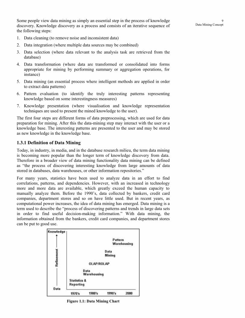
Spatial Databases

Spatial databases are databases that, in addition to usual data, store geographical

information like maps, and global or regional positioning. Such spatial databases

present new challenges to data mining algorithms.

Figure 1.5: Visualisation of Spatial OLAP

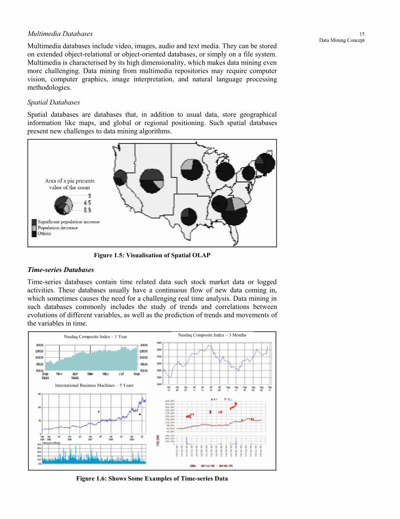
Time-series Databases

Time-series databases contain time related data such stock market data or logged

activities. These databases usually have a continuous flow of new data coming in,

which sometimes causes the need for a challenging real time analysis. Data mining in

such databases commonly includes the study of trends and correlations between

evolutions of different variables, as well as the prediction of trends and movements of

the variables in time.

Figure 1.6: Shows Some Examples of Time-series Data

Nasdaq Composite Index – 1 Year

International Business Machines – 5 Years

Nasdaq Composite Index – 3 Months

16


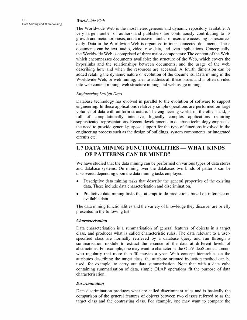
Worldwide Web

The Worldwide Web is the most heterogeneous and dynamic repository available. A

very large number of authors and publishers are continuously contributing to its

growth and metamorphosis, and a massive number of users are accessing its resources

daily. Data in the Worldwide Web is organised in inter-connected documents. These

documents can be text, audio, video, raw data, and even applications. Conceptually,

the Worldwide Web is comprised of three major components: The content of the Web,

which encompasses documents available; the structure of the Web, which covers the

hyperlinks and the relationships between documents; and the usage of the web,

describing how and when the resources are accessed. A fourth dimension can be

added relating the dynamic nature or evolution of the documents. Data mining in the

Worldwide Web, or web mining, tries to address all these issues and is often divided

into web content mining, web structure mining and web usage mining.

Engineering Design Data

Database technology has evolved in parallel to the evolution of software to support

engineering. In these applications relatively simple operations are performed on large

volumes of data with uniform structure. The engineering world, on the other hand, is

full of computationally intensive, logically complex applications requiring

sophisticated representations. Recent developments in database technology emphasise

the need to provide general-purpose support for the type of functions involved in the

engineering process such as the design of buildings, system components, or integrated

circuits etc.

1.7 DATA MINING FUNCTIONALITIES — WHAT KINDS

OF PATTERNS CAN BE MINED?

We have studied that the data mining can be performed on various types of data stores

and database systems. On mining over the databases two kinds of patterns can be

discovered depending upon the data mining tasks employed:

Descriptive data mining tasks that describe the general properties of the existing

data. These include data characterisation and discrimination.

Predictive data mining tasks that attempt to do predictions based on inference on

available data.

The data mining functionalities and the variety of knowledge they discover are briefly

presented in the following list:

Characterisation

Data characterisation is a summarisation of general features of objects in a target

class, and produces what is called characteristic rules. The data relevant to a user-

specified class are normally retrieved by a database query and run through a

summarisation module to extract the essence of the data at different levels of

abstractions. For example, one may want to characterise the OurVideoStore customers

who regularly rent more than 30 movies a year. With concept hierarchies on the

attributes describing the target class, the attribute oriented induction method can be

used, for example, to carry out data summarisation. Note that with a data cube

containing summarisation of data, simple OLAP operations fit the purpose of data

characterisation.

Discrimination

Data discrimination produces what are called discriminant rules and is basically the

comparison of the general features of objects between two classes referred to as the

target class and the contrasting class. For example, one may want to compare the

17

Data Mining Concept general characteristics of the customers who rented more than 30 movies in the last

year with those whose rental account is lower than 5. The techniques used for data

discrimination are very similar to the techniques used for data characterisation with

the exception that data discrimination results include comparative measures.

Association Analysis

Association analysis is based on the association rules. It studies the frequency of items

occurring together in transactional databases, and based on a threshold called support,

identifies the frequent item sets. Another threshold, confidence, which is the

conditional probability than an item appears in a transaction when another item

appears, is used to pinpoint association rules. Association analysis is commonly used

for market basket analysis. For example, it could be useful for the OurVideoStore

manager to know what movies are often rented together or if there is a relationship

between renting a certain type of movies and buying popcorn or pop. The discovered

association rules are of the form: P→Q [s, c], where P and Q are conjunctions of

attribute value-pairs, and s (for support) is the probability that P and Q appear together

in a transaction and c (for confidence) is the conditional probability that Q appears in

a transaction when P is present. For example, the hypothetic association rule

Rent Type (X, “game”) ٨ Age(X,“13-19”) → Buys(X, “pop”) [s = 2%, c = 55%]

would indicate that 2% of the transactions considered are of customers aged between

13 and 19 who are renting a game and buying a pop, and that there is a certainty of

55% that teenage customers, who rent a game, also buy pop.

Classification

Classification is the processing of finding a set of models (or functions) that describe

and distinguish data classes or concepts, for the purposes of being able to use the

model to predict the class of objects whose class label is unknown. The derived model

is based on the analysis of a set of training data (i.e., data objects whose class label is

known). The derived model may be represented in various forms, such as

classification (IF-THEN) rules, decision trees, mathematical formulae, or neural

networks. For example, after starting a credit policy, the Our Video Store managers

could analyse the customers’ behaviors vis-à-vis their credit, and label accordingly the

customers who received credits with three possible labels “safe”, “risky” and “very

risky”. The classification analysis would generate a model that could be used to either

accept or reject credit requests in the future.

Prediction

Classification can be used for predicting the class label of data objects. There are two

major types of predictions: one can either try to predict (1) some unavailable data

values or pending trends and (2) a class label for some data. The latter is tied to

classification. Once a classification model is built based on a training set, the class

label of an object can be foreseen based on the attribute values of the object and the

attribute values of the classes. Prediction is however more often referred to the

forecast of missing numerical values, or increase/ decrease trends in time related data.

The major idea is to use a large number of past values to consider probable future

values.

Note that Classification and prediction may need to be preceded by relevance analysis,

which attempts to identify attributes that do not contribute to the classification or

prediction process. These attributes can then be excluded.

Clustering

Similar to classification, clustering is the organisation of data in classes. However,

unlike classification, it is used to place data elements into related groups without

18


advance knowledge of the group definitions i.e. class labels are unknown and it is up

to the clustering algorithm to discover acceptable classes. Clustering is also called

unsupervised classification, because the classification is not dictated by given class

labels. There are many clustering approaches all based on the principle of maximising

the similarity between objects in a same class (intra-class similarity) and minimising

the similarity between objects of different classes (inter-class similarity). Clustering

can also facilitate taxonomy formation, that is, the organisation of observations into a

hierarchy of classes that group similar events together. For example, for a data set

with two attributes: AGE and HEIGHT, the following rule represents most of the data

assigned to cluster 10:

If AGE >= 25 and AGE <= 40 and HEIGHT >= 5.0ft and HEIGHT <= 5.5ft then

CLUSTER = 10

Evolution and Deviation Analysis

Evolution and deviation analysis pertain to the study of time related data that changes

in time.

Evolution analysis models evolutionary trends in data, which consent to

characterising, comparing, classifying or clustering of time related data. For example,

suppose that you have the major stock market (time-series) data of the last several

years available from the New York Stock Exchange and you would like to invest in

shares of high-tech industrial companies. A data mining study of stock exchange data

may identify stock evolution regularities for overall stocks and for the stocks of

particular companies. Such regularities may help predict future trends in stock market

prices, contributing to your decision-making regarding stock investment.

Deviation analysis, on the other hand, considers differences between measured values

and expected values, and attempts to find the cause of the deviations from the

anticipated values. For example, a decrease in total demand of CDs for rent at Video

library for the last month, in comparison to that of the same month of the last year, is a

deviation pattern. Having detected a significant deviation, a data mining system may

go further and attempt to explain the detected pattern (e.g., did the new comedy

movies were released last year in comparison to the same period this year?).


Write short notes on the following:

1. Data warehouses.

……………………….……………………….…………………………….

……………………….……………………….…………………………….

2. Transaction databases.

……………………….……………………….…………………………….

……………………….……………………….…………………………….

1.8 CLASSIFICATION OF DATA MINING SYSTEMS

There are many data mining systems available or being developed. Some are

specialised systems dedicated to a given data source or are confined to limited data

mining functionalities, other are more versatile and comprehensive. Data mining

systems can be categorised according to various criteria among other classification are

the following:

Classification according to the kinds of data source mined: this classification

categorises data mining systems according to the type of data handled such as

spatial data, multimedia data, time-series data, text data, Worldwide Web, etc.

19

Data Mining Concept Classification according to the data model drawn on: this classification

categorises data mining systems based on the data model involved such as

relational database, object-oriented database, data warehouse, transactional, etc.

Classification according to the kind of knowledge discovered: this classification

categorises data mining systems based on the kind of knowledge discovered or

data mining functionalities, such as characterisation, discrimination, association,

classification, clustering, etc. Some systems tend to be comprehensive systems

offering several data mining functionalities together.

Classification according to mining techniques used: Data mining systems

employ and provide different techniques. This classification categorises data

mining systems according to the data analysis approach used such as machine

learning, neural networks, genetic algorithms, statistics, visualisation, database-

oriented or data warehouse-oriented, etc. The classification can also take into

account the degree of user interaction involved in the data mining process such as

query-driven systems, interactive exploratory systems, or autonomous systems. A

comprehensive system would provide a wide variety of data mining techniques to

fit different situations and options, and offer different degrees of user interaction.

1.9 ADVANTAGES OF DATA MINING

Advantages of Data Mining from different point of view are:

Marketing/Retailing

Data mining can aid direct marketers by providing them with useful and accurate

trends about their customers’ purchasing behavior. Based on these trends, marketers

can direct their marketing attentions to their customers with more precision. For

example, marketers of a software company may advertise about their new software to

consumers who have a lot of software purchasing history. In addition, data mining

may also help marketers in predicting which products their customers may be

interested in buying. Through this prediction, marketers can surprise their customers

and make the customer’s shopping experience becomes a pleasant one.

Retail stores can also benefit from data mining in similar ways. For example, through

the trends provide by data mining, the store managers can arrange shelves, stock

certain items, or provide a certain discount that will attract their customers.

Banking/Crediting

Data mining can assist financial institutions in areas such as credit reporting and loan

information. For example, by examining previous customers with similar attributes, a

bank can estimated the level of risk associated with each given loan. In addition, data

mining can also assist credit card issuers in detecting potentially fraudulent credit card

transaction. Although the data mining technique is not a 100% accurate in its

prediction about fraudulent charges, it does help the credit card issuers reduce their

losses.

Law Enforcement

Data mining can aid law enforcers in identifying criminal suspects as well as

apprehending these criminals by examining trends in location, crime type, habit, and

other patterns of behaviors.

Researchers

Data mining can assist researchers by speeding up their data analyzing process; thus,

allowing them more time to work on other projects.

20


1.10 DISADVANTAGES OF DATA MINING

Disadvantages of Data Mining are:

Privacy Issues

Personal privacy has always been a major concern in this country. In recent years,

with the widespread use of Internet, the concerns about privacy have increase

tremendously. Because of the privacy issues, some people do not shop on Internet.

They are afraid that somebody may have access to their personal information and then

use that information in an unethical way; thus causing them harm.

Although it is against the law to sell or trade personal information between different

organizations, selling personal information have occurred. For example, according to

Washing Post, in 1998, CVS had sold their patient’s prescription purchases to a

different company. In addition, American Express also sold their customers’ credit

care purchases to another company. What CVS and American Express did clearly

violate privacy law because they were selling personal information without the

consent of their customers. The selling of personal information may also bring harm

to these customers because you do not know what the other companies are planning to

do with the personal information that they have purchased.

Security Issues

Although companies have a lot of personal information about us available online, they

do not have sufficient security systems in place to protect that information. For

example, recently the Ford Motor credit company had to inform 13,000 of the

consumers that their personal information including Social Security number, address,

account number and payment history were accessed by hackers who broke into a

database belonging to the Experian credit reporting agency. This incidence illustrated

that companies are willing to disclose and share your personal information, but they

are not taking care of the information properly. With so much personal information

available, identity theft could become a real problem.

Misuse of Information/inaccurate Information

Trends obtain through data mining intended to be used for marketing purpose or for

some other ethical purposes, may be misused. Unethical businesses or people may

used the information obtained through data mining to take advantage of vulnerable

people or discriminated against a certain group of people. In addition, data mining

technique is not a 100 percent accurate; thus mistakes do happen which can have

serious consequence.

1.11 ETHICAL ISSUES OF DATA MINING

As with many technologies, both positives and negatives lie in the power of data

mining. There are, of course, valid arguments to both sides. Here is the positive as

well as the negative things about data mining from different perspectives.

1.11.1 Consumers’ Point of View

According to the consumers, data mining benefits businesses more than it benefit

them. Consumers may benefit from data mining by having companies customized

their product and service to fit the consumers’ individual needs. However, the

consumers’ privacy may be lost as a result of data mining.

Data mining is a major way that companies can invade the consumers’ privacy.

Consumers are surprised as how much companies know about their personal lives. For

example, companies may know your name, address, birthday, and personal

information about your family such as how many children you have. They may also

21

Data Mining Concept know what medications you take, what kind of music you listen to, and what are your

favorite books or movies. The lists go on and on. Consumers are afraid that these

companies may misuse their information, or not having enough security to protect

their personal information from unauthorized access. For example, the incidence

about the hackers in the Ford Motor company case illustrated how insufficient

companies are at protecting their customers’ personal information. Companies are

making profits from their customers’ personal data, but they do not want to spend a lot

amount of money to design a sophisticated security system to protect that data. At

least half of Internet users interviewed by Statistical Research, Inc. claimed that they

were very concerned about the misuse of credit care information given online, the

selling or sharing of personal information by different web sites and cookies that track

consumers’ Internet activity.

Data mining that allows companies to identify their best customers could just be easily

used by unscrupulous businesses to attack vulnerable customer such as the elderly, the

poor, the sick, or the unsophisticated people. These unscrupulous businesses could use

the information unethically by offering these vulnerable people inferior deals. For

example, Mrs. Smith’s husband was diagnosis with colon cancer, and the doctor

predicted that he is going to die soon. Mrs. Smith was so worry and depressed.

Suppose through Mrs. Smith’s participation in a chat room or mailing list, someone

predicts that either she or someone close to her has a terminal illness. Maybe through

this prediction, Mrs. Smith started receiving email from some strangers stating that

they know a cure for colon cancer, but it will cause her a lot of money. Mrs. Smith

who is desperately wanted to save her husband, may fall into their trap. This

hypothetical example illustrated that how unethical it is for somebody to use data

obtained through data mining to target vulnerable person who are desperately hoping

for a miracle.

Data mining can also be used to discriminate against a certain group of people in the

population. For example, if through data mining, a certain group of people were

determine to carry a high risk for a deathly disease (e.g. HIV, cancer), then the

insurance company may refuse to sell insurance policy to them based on this

information. The insurance company’s action is not only unethical, but may also have

severe impact on our health care system as well as the individuals involved. If these

high risk people cannot buy insurance, they may die sooner than expected because

they cannot afford to go to the doctor as often as they should. In addition, the

government may have to step in and provide insurance coverage for those people, thus

would drive up the health care costs.

Data mining is not a flawless process, thus mistakes are bound to happen. For

example, a file of one person may get mismatch to another person file. In today world,

where we replied heavily on the computer for information, a mistake generated by the

computer could have serious consequence. One may ask is it ethical for someone with

a good credit history to get reject for a loan application because his/her credit history

get mismatched with someone else bearing the same name and a bankruptcy profile?

The answer is “NO” because this individual does not do anything wrong. However, it

may take a while for this person to get his file straighten out. In the mean time, he or

she just has to live with the mistake generated by the computer. Companies might say

that this is an unfortunate mistake and move on, but to this individual this mistake can

ruin his/her life.

1.11.2 Organizations’ Point of View

Data mining is a dream comes true to businesses because data mining helps enhance

their overall operations and discover new patterns that may allow companies to better

serve their customers. Through data mining, financial and insurance companies are

able to detect patterns of fraudulent credit care usage, identify behavior patterns of

risk customers, and analyze claims. Data mining would help these companies

22


minimize their risk and increase their profits. Since companies are able to minimize

their risk, they may be able to charge the customers lower interest rate or lower

premium. Companies are saying that data mining is beneficial to everyone because

some of the benefit that they obtained through data mining will be passed on to the

consumers.

Data mining also allows marketing companies to target their customers more

effectively; thus, reducing their needs for mass advertisements. As a result, the

companies can pass on their saving to the consumers. According to Michael Turner,

an executive director of a Directing Marking Association “Detailed consumer

information lets apparel retailers market their products to consumers with more

precision. But if privacy rules impose restrictions and barriers to data collection, those

limitations could increase the prices consumers pay when they buy from catalog or

online apparel retailers by 3.5% to 11%”.

When it comes to privacy issues, organizations are saying that they are doing

everything they can to protect their customers’ personal information. In addition, they

only use consumer data for ethical purposes such as marketing, detecting credit card

fraudulent, and etc. To ensure that personal information are used in an ethical way, the

chief information officers (CIO) Magazine has put together a list of what they call the

Six Commandments of Ethical Date Management. The six commandments include:

Data is a valuable corporate asset and should be managed as such, like cash,

facilities or any other corporate asset;

The CIO is steward of corporate data and is responsible for managing it over its

life cycle (from its generation to its appropriate destruction);

The CIO is responsible for controlling access to and use of data, as determined by

governmental regulation and corporate policy;

The CIO is responsible for preventing inappropriate destruction of data;

The CIO is responsible for bringing technological knowledge to the development

of data management practices and policies;

The CIO should partner with executive peers to develop and execute the

organization’s data management policies.

Since data mining is not a perfect process, mistakes such as mismatching information

do occur. Companies and organizations are aware of this issue and try to deal it.

According to Agrawal, a IBM’s researcher, data obtained through mining is only

associated with a 5 to 10 percent loss in accuracy. However, with continuous

improvement in data mining techniques, the percent in inaccuracy will decrease

significantly.

1.11.3 Government’s Point of View

The government is in dilemma when it comes to data mining practices. On one hand,

the government wants to have access to people’s personal data so that it can tighten

the security system and protect the public from terrorists, but on the other hand, the

government wants to protect the people’s privacy right. The government recognizes

the value of data mining to the society, thus wanting the businesses to use the

consumers’ personal information in an ethical way. According to the government, it is

against the law for companies and organizations to trade data they had collected for

money or data collected by another organization. In order to protect the people’s

privacy right, the government wants to create laws to monitor the data mining

practices. However, it is extremely difficult to monitor such disparate resources as

servers, databases, and web sites. In addition, Internet is global, thus creating

tremendous difficulty for the government to enforce the laws.

23

Data Mining Concept 1.11.4 Society’s Point of View

Data mining can aid law enforcers in their process of identify criminal suspects and

apprehend these criminals. Data mining can help reduce the amount of time and effort

that these law enforcers have to spend on any one particular case. Thus, allowing them

to deal with more problems. Hopefully, this would make the country becomes a safer

place. In addition, data mining may also help reduce terrorist acts by allowing

government officers to identify and locate potential terrorists early. Thus, preventing

another incidence likes the World Trade Center tragedy from occurring on American

soil.

Data mining can also benefit the society by allowing researchers to collect and

analyze data more efficiently. For example, it took researchers more than a decade to

complete the Human Genome Project. But with data mining, similar projects could be

completed in a shorter amount of time. Data mining may be an important tool that aid

researchers in their search for new medications, biological agents, or gene therapy that

would cure deadly diseases such as cancers or AIDS.

1.12 ANALYSIS OF ETHICAL ISSUES

After looking at different views about data mining, one can see that data mining

provides tremendous benefit to businesses, governments, and society. Data mining is

also beneficial to individual persons, however, this benefit is minor compared to the

benefits obtain for the companies. In addition, in order to gain this benefit, individual

persons have to give up a lot of their privacy right.

If we choose to support data mining, then it would be unfair to the consumers because

their right of privacy may be violated. Currently, business organizations do not have

sufficient security systems to protect the personal information that they obtained

through data mining from unauthorized access. Utilitarian, however, would supported

this view because according to them, “An action is right from ethical point of view, if

and only if, the sum total of utilities produced by that act is greater than the sum total

of utilities produced by any other act the agent could have performed in its place.”

From the utilitarian view, data mining is a good thing because it enables corporations

to minimize risk and increases profit; helps the government strengthen the security

system; and benefit the society by speeding up the technological advancement. The

only downside to data mining is the invasion of personal privacy and the risk of

having people misuse the data. Based on this theory, since the majority of the party

involves benefit from data mining, then the use of data mining is morally right.

If we choose to restrict data mining, then it would be unfair to the businesses and the

government that use data mining in an ethical way. Restricting data mining would

affect businesses’ profits, national security, and may cause a delay in the discovery of

new medications, biological agents, or gene therapy that would cure deadly diseases

such as cancers or AIDS. Kant’s categorical imperative, however, would supported

this view because according to him “An action is morally right for a person if, and

only if, in performing the action, the person does not use others merely as a means for

advancing his or her own interests, but also both respects and develops their capacity

to choose freely for themselves.” From Kant’s view, the use of data mining is

unethical because the corporation and the government to some extent used data

mining to advance their own interests without regard for people’s privacy. With so

many web sites being hack and private information being stolen, the benefit obtained

through data mining is not good enough to justify the risk of privacy invasion.

As people collect and centralize data to a specific location, there always existed a

chance that these data may be hacked by someone sooner or later. Businesses always

promise they would treat the data with great care and guarantee the information will

be save. But time after time, they have failed to keep their promise. So until

companies able to develop better security system to safeguard consumer data against

24


unauthorized access, the use of data mining should be restricted because there is no

benefit that can outweigh the safety and wellbeing of any human being.

1.13 GLOBAL ISSUES OF DATA MINING

Since we are living in an Internet era, data mining will not only affect the US, instead

it will have a global impact. Through Internet, a person living in Japan or Russia may

have access to the personal information about someone living in California. In recent

years, several major international hackers have break into US companies stealing

hundred of credit card numbers. These hackers have used the information that they

obtained through hacking for credit card fraud, black mailing purpose, or selling credit

card information to other people. According to the FBI, the majority of the hackers are

from Russia and the Ukraine. Though, it is not surprised to find that the increase in

fraudulent credit card usage in Russian and Ukraine is corresponded to the increase in

domestic credit card theft.

After the hackers gained access to the consumer data, they usually notify the victim

companies of the intrusion or theft, and either directly demanded the money or offer to

patch the system for a certain amount of money. In some cases, when the companies

refuse to make the payments or hire them to fix system, the hackers have release the

credit card information that they previous obtained onto the Web. For example, a

group of hackers in Russia had attacked and stolen about 55,000 credit card numbers

from merchant card processor CreditCards.com. The hackers black mailed the

company for $ 100,000, but the company refused to pay. As a result, the hackers

posted almost half of the stolen credit card numbers onto the Web. The consumers

whose card numbers were stolen incurred unauthorized charges from a Russian-based

site. Similar problem also happened to CDUniverse.com in December 1999. In this

case, a Russian teenager hacked into CDUniverse.com site and stolen about 300,000

credit card numbers. This teenager, like the group mentioned above also demanded

$100,000 from CDUniverse.com. CDUniverse.com refused to pay and again their

customers’ credit card numbers were released onto the Web called the Maxus credit

card pipeline.

Besides hacking into e-commerce companies to steal their data, some hackers just

hack into a company for fun or just trying to show off their skills. For example, a

group of hacker called “BugBear” had hacked into a security consulting company’s

website. The hackers did not stole any data from this site, instead they leave a

message like this “It was fun and easy to break into your box.”

Besides the above cases, the FBI is saying that in 2001, about 40 companies located in

20 different states have already had their computer systems accessed by hackers.

Since hackers can hack into the US e-commerce companies, then they can hack into

any company worldwide. Hackers could have a tremendous impact on online

businesses because they scared the consumers from purchasing online. Major hacking

incidences liked the two mentioned above illustrated that the companies do not have

sufficient security system to protect customer data. More efforts are needed from the

companies as well as the government to tighten security against these hackers. Since

the Internet is global, efforts from different governments worldwide are needed.

Different countries need to join hand and work together to protect the privacy of their

people.

1.14 LET US SUM UP

The information and knowledge gained can be used for applications ranging from

business management, production control, and market analysis, to engineering design

and science exploration. Data mining can be viewed as a result of the natural

evolution of information technology. An evolutionary path has been witnessed in the

database industry in the development of data collection and database creation, data

management and data analysis functionalities. Data mining refers to extracting or

25

Data Mining Concept "mining" knowledge from large amounts of data. Some other terms like knowledge

mining from data, knowledge extraction, data/pattern analysis, data archaeology, and

data dredging are also used for data mining. Knowledge discovery as a process and

consists of an iterative sequence of the data cleaning, data integration, data selection

data transformation, data mining, pattern evaluation and knowledge presentation.

1.15 LESSON END ACTIVITY

Discuss how data mining works? Also discuss how you manage the data warehouse

for a manufacturing organization.

1.16 KEYWORDS

Data Mining: It refers to extracting or "mining" knowledge from large amounts of

data.

KDD: Many people treat data mining as a synonym for another popularly used term,

Knowledge Discovery from Data, or KDD.

Data Cleaning: To remove noise and inconsistent data.

Data Integration: Multiple data sources may be combined.

Data Selection: Data relevant to the analysis task are retrieved from the database.

Data Transformation: Where data are transformed or consolidated into forms

appropriate for mining by performing summary or aggregation operations.

1.17 QUESTIONS FOR DISCUSSION

1. What is data mining?

2. Why data mining is crucial to the success of a business?

3. Write down the differences and similarities between a database and a data

warehouse.

4. Define each of the following data mining functionalities: characterisation,

discrimination, association, classification, prediction, clustering, and evolution

and deviation analysis.

5. What is the difference between discrimination and classification?

Check Your Progress: Model Answers

CYP 1

1. The process of discovering interesting knowledge from large amounts of

data stored in databases, data warehouses, or other information

repositories.

2. (a) Information repository

(b) Database or data warehouse server

(c) Knowledge base

CYP 2

1. A data warehouse is a repository of information collected from multiple

sources, stored under a unified schema, and that usually resides at a single

site. Data warehouses are constructed via a process of data cleaning, data

integration, data transformation, data loading, and periodic data

refreshing.

2. A transaction database is a set of records representing transactions, each

with a time stamp, an identifier and a set of items. Associated with the

transaction files could also be descriptive data for the items.

26


1.18 SUGGESTED READINGS

Usama Fayyad, Gregory Piatetsky-Shapiro, Padhraic Smyth, and Ramasamy Uthurasamy,

“Advances in Knowledge Discovery and Data Mining”, AAAI Press/The MIT Press, 1996.

J. Ross Quinlan, “C4.5: Programs for Machine Learning”, Morgan Kaufmann Publishers,

1993.

Michael Berry and Gordon Linoff, “Data Mining Techniques” (For Marketing, Sales, and

Customer Support), John Wiley & Sons, 1997.

Sholom M. Weiss and Nitin Indurkhya, “Predictive Data Mining: A Practical Guide”, Morgan

Kaufmann Publishers, 1998.

Alex Freitas and Simon Lavington, “Mining Very Large Databases with Parallel Processing”,

Kluwer Academic Publishers, 1998.

A.K. Jain and R.C. Dubes, “Algorithms for Clustering Data”, Prentice Hall, 1988.

V. Cherkassky and F. Mulier, “Learning from Data”, John Wiley & Sons, 1998.

Jiawei Han, Micheline Kamber, Data Mining – Concepts and Techniques, Morgan Kaufmann

Publishers, 1st Edition, 2003.

Michael J.A. Berry, Gordon S Linoff, Data Mining Techniques, Wiley Publishing Inc, Second

Edition, 2004.

Alex Berson, Stephen J. Smith, Data warehousing, Data Mining & OLAP, Tata McGraw Hill,

Publications, 2004.

Sushmita Mitra, Tinku Acharya, Data Mining – Multimedia, Soft Computing and

Bioinformatics, John Wiley & Sons, 2003.

Sam Anohory, Dennis Murray, Data Warehousing in the Real World, Addison Wesley, First

Edition, 2000.

27

Data Mining with Database LESSON

2 DATA MINING WITH DATABASE

CONTENTS


2.1 Introduction

2.2 Data Mining Technology

2.3 Data Mining and Knowledge Discovery in Databases

2.3.1 History of Data Mining and KDD

2.3.2 Data Mining versus KDD

2.4 KDD Basic Definition

2.5 KDD Process

2.6 Data Mining Issues

2.7 Data Mining Metrices

2.8 Social Implication of Data Mining

2.9 Data Mining from a Database Perspective

2.10 Let us Sum up


2.12 Keywords





Concept of data mining

Concept of knowledge discovery in database

Basic knowledge of data mining metrices

Data mining from a database perspective

2.1 INTRODUCTION

Data mining is emerging as a rapidly growing interdisciplinary field that takes its

approach from different areas like, databases, statistics, artificial intelligence and data

structures in order to extract hidden knowledge from large volumes of data. The data

mining concept is now a days not only used by the research community but also a lot

of companies are using it for predictions so that, they can compete and stay ahead of

their competitors.

28


With rapid computerisation in the past two decades, almost all organisations have

collected huge amounts of data in their databases. These organisations need to

understand their data and also want to discover useful knowledge as patterns, from

their existing data.

2.2 DATA MINING TECHNOLOGY

Data is growing at a phenomenal rate today and the users expect more sophisticated

information from this data. There is need for new techniques and tools that can

automatically generate useful information and knowledge from large volumes of data.

Data mining is one such technique of generating hidden information from the data.

Data mining can be defined as: “an automatic process of extraction of non-trivial or

implicit or previously unknown but potentially useful information or patterns from

data in large databases, data warehouses or in flat files”.

Data mining is related to data warehouse in this respect that, a data warehouse is well

equipped for providing data as input for the data mining process. The advantages of

using the data of data warehouse for data mining are or many some of them are listed

below:

Data quality and consistency are essential for data mining, to ensure, the accuracy

of the predictive models. In data warehouses, before loading the data, it is first

extracted, cleaned and transformed. We will get good results only if we have good

quality data.

Data warehouse consists of data from multiple sources. The data in data

warehouses is integrated and subject oriented data. The data mining process

performed on this data.

In data mining, it may be the case that, the required data may be aggregated or

summarised data. This is already there in the data warehouse.

Data warehouse provides the capability of analysing data by using OLAP

operations. Thus, the results of a data mining study can be analysed for hirtherto,

uncovered patterns.

2.3 DATA MINING AND KNOWLEDGE DISCOVERY

IN DATABASES

Data mining and knowledge discovery in databases have been attracting a significant

amount of research, industry, and media attention of late. What is all the excitement

about? Across a wide variety of fields, data are being collected and accumulated at a

dramatic pace. There is an urgent need for a new generation of computational theories

and tools to assist humans in extracting useful information (knowledge) from the

rapidly growing volumes of digital data. These theories and tools are the subject of the

emerging field of knowledge discovery in databases (KDD).

Why do we need KDD?

The traditional method of turning data into knowledge relies on manual analysis and

interpretation. For example, in the health-care industry, it is common for specialists to

periodically analyze current trends and changes in health-care data, say, on a quarterly

basis. The specialists then provide a report detailing the analysis to the sponsoring

health-care organization; this report becomes the basis for future decision making and

planning for health-care management. In a totally different type of application,

planetary geologists sift through remotely sensed images of planets and asteroids,

carefully locating and cataloging such geologic objects of interest as impact craters.

Be it science, marketing, finance, health care, retail, or any other field, the classical

approach to data analysis relies fundamentally on one or more analysts becoming

29

Data Mining with Database intimately familiar with the data and serving as an interface between the data and the

users and products.

For these (and many other) applications, this form of manual probing of a data set is

slow, expensive, and highly subjective. In fact, as data volumes grow dramatically,

this type of manual data analysis is becoming completely impractical in many

domains.

Databases are increasing in size in two ways: (1) the number N of records or objects

in the database and (2) the number d of fields or attributes to an object. Databases

containing on the order of N = 109 objects are becoming increasingly common, for

example, in the astronomical sciences. Similarly, the number of fields d can easily be

on the order of 102 or even 103, for example, in medical diagnostic applications. Who

could be expected to digest millions of records, each having tens or hundreds of

fields? We believe that this job is certainly not one for humans; hence, analysis work

needs to be automated, at least partially. The need to scale up human analysis

capabilities to handling the large number of bytes that we can collect is both economic

and scientific. Businesses use data to gain competitive advantage, increase efficiency,

and provide more valuable services to customers. Data we capture about our

environment are the basic evidence we use to build theories and models of the

universe we live in. Because computers have enabled humans to gather more data than

we can digest, it is only natural to turn to computational techniques to help us unearth

meaningful patterns and structures from the massive volumes of data. Hence, KDD is

an attempt to address a problem that the digital information era made a fact of life for

all of us: data overload.

Data Mining and Knowledge Discovery in the Real World

In business, main KDD application areas includes marketing, finance (especially

investment), fraud detection, manufacturing, telecommunications, and Internet agents.

Marketing: In marketing, the primary application is database marketing systems,

which analyze customer databases to identify different customer groups and forecast

their behavior. Business Week (Berry 1994) estimated that over half of all retailers are

using or planning to use database marketing, and those who do use it have good

results; for example, American Express reports a 10- to 15- percent increase in credit-

card use. Another notable marketing application is market-basket analysis (Agrawal

et al. 1996) systems, which find patterns such as, “If customer bought X, he/she is

also likely to buy Y and Z.” Such patterns are valuable to retailers.

Investment: Numerous companies use data mining for investment, but most do not

describe their systems. One exception is LBS Capital Management. Its system uses

expert systems, neural nets, and genetic algorithms to manage portfolios totaling $600

million; since its start in 1993, the system has outperformed the broad stock market.

Fraud detection: HNC Falcon and Nestor PRISM systems are used for monitoring

credit card fraud, watching over millions of accounts. The FAIS system (Senator

et al. 1995), from the U.S. Treasury Financial Crimes Enforcement Network, is used

to identify financial transactions that might indicate money laundering activity.

Manufacturing: The CASSIOPEE troubleshooting system, developed as part of a

joint venture between General Electric and SNECMA, was applied by three major

European airlines to diagnose and predict problems for the Boeing 737. To derive

families of faults, clustering methods are used. CASSIOPEE received the European

first prize for innovative applications.

Telecommunications: The telecommunications alarm-sequence analyzer (TASA) was

built in cooperation with a manufacturer of telecommunications equipment and three

telephone networks (Mannila, Toivonen, and Verkamo 1995). The system uses a

novel framework for locating frequently occurring alarm episodes from the alarm

30


stream and presenting them as rules. Large sets of discovered rules can be explored

with flexible information- retrieval tools supporting interactivity and iteration. In this

way, TASA offers pruning, grouping, and ordering tools to refine the results of a basic

brute-force search for rules.

Data cleaning: The MERGE-PURGE system was applied to the identification of

duplicate welfare claims (Hernandez and Stolfo 1995). It was used successfully on

data from the Welfare Department of the State of Washington.

In other areas, a well-publicized system is IBM’s ADVANCED SCOUT, a specialized

data-mining system that helps National Basketball Association (NBA) coaches

organize and interpret data from NBA games (U.S. News 1995). ADVANCED

SCOUT was used by several of the NBA teams in 1996, including the Seattle

Supersonics, which reached the NBA finals.

2.3.1 History of Data Mining and KDD

Historically, the notion of finding useful patterns in data has been given a variety of

names, including data mining, knowledge extraction, information discovery,

information harvesting, data archaeology, and data pattern processing. The term data

mining has mostly been used by statisticians, data analysts, and the management

information systems (MIS) communities. It has also gained popularity in the database

field. The phrase knowledge discovery in databases was coined at the first KDD

workshop in 1989 (Piatetsky-Shapiro 1991) to emphasize that knowledge is the end

product of a data-driven discovery. It has been popularized in the AI and machine-

learning fields.

KDD refers to the overall process of discovering useful knowledge from data, and

data mining refers to a particular step in this process. Data mining is the application of

specific algorithms for extracting patterns from data. The distinction between the

KDD process and the data-mining step (within the process) is a central point of this

article. The additional steps in the KDD process, such as data preparation, data

selection, data cleaning, incorporation of appropriate prior knowledge, and proper

interpretation of the results of mining, are essential to ensure that useful knowledge is

derived from the data. Blind application of data-mining methods (rightly criticized as

data dredging in the statistical literature) can be a dangerous activity, easily leading to

the discovery of meaningless and invalid patterns.

2.3.2 Data Mining versus KDD

Knowledge Discovery in Databases (KDD) is the process of finding useful

information, knowledge and patterns in data while data mining is the process of using

of algorithms to automatically extract desired information and patterns, which are

derived by the Knowledge Discovery in Databases process.

2.4 KDD BASIC DEFINITION

KDD is the non-trivial process of identifying valid, novel, potentially useful, and

ultimately understandable patterns in data.

Data are a set of facts (for example, cases in a database), and pattern is an expression

in some language describing a subset of the data or a model applicable to the subset.

Hence, in our usage here, extracting a pattern also designates fitting a model to data;

finding structure from data; or, in general, making any high-level description of a set

of data. The term process implies that KDD comprises many steps, which involve data

preparation, search for patterns, knowledge evaluation, and refinement, all repeated in

multiple iterations. By non-trivial, we mean that some search or inference is involved;

that is, it is not a straightforward computation of predefined quantities like computing

the average value of a set of numbers.

31

Data Mining with Database The discovered patterns should be valid on new data with some degree of certainty.

We also want patterns to be novel (at least to the system and preferably to the user)

and potentially useful, that is, lead to some benefit to the user or task. Finally, the

patterns should be understandable, if not immediately then after some post-processing.

Data mining is a step in the KDD process that consists of applying data analysis and

discovery algorithms that, under acceptable computational efficiency limitations,

produce a particular enumeration of patterns (or models) over the data. Note that the

space of patterns is often infinite, and the enumeration of patterns involves some form

of search in this space. Practical computational constraints place severe limits on the

subspace that can be explored by a data-mining algorithm.

The KDD process involves using the database along with any required selection,

preprocessing, subsampling, and transformations of it; applying data-mining methods

(algorithms) to enumerate patterns from it; and evaluating the products of data mining

to identify the subset of the enumerated patterns deemed knowledge. The data-mining

component of the KDD process is concerned with the algorithmic means by

which patterns are extracted and enumerated from data. The overall KDD process

(Figure 2.1) includes the evaluation and possible interpretation of the mined patterns

to determine which patterns can be considered new knowledge.

Figure 2.1: An Overview of the Steps that Compose the KDD Process

2.5 KDD PROCESS

The KDD process is interactive and iterative, involving numerous steps with many

decisions made by the user. Brachman and Anand (1996) give a practical view of the

KDD process, emphasizing the interactive nature of the process. Here, we broadly

outline some of its basic steps:

Developing an understanding of the application domain and the relevant prior

knowledge and identifying the goal of the KDD process from the customer’s

viewpoint.

Creating a target data set: selecting a data set, or focusing on a subset of

variables or data samples, on which discovery is to be performed.

Data cleaning and preprocessing. Basic operations include removing noise if

appropriate, collecting the necessary information to model or account for noise,

deciding on strategies for handling missing data fields, and accounting for time-

sequence information and known changes.

Data reduction and projection: finding useful features to represent the data

depending on the goal of the task. With dimensionality reduction or

transformation methods, the effective number of variables under consideration can

be reduced, or invariant representations for the data can be found.

32


Matching the goals of the KDD process (step 1) to a particular data-mining

method. For example, summarization, classification, regression, clustering, and so

on.

Exploratory analysis and model and hypothesis selection: choosing the data

mining algorithm(s) and selecting method(s) to be used for searching for data

patterns. This process includes deciding which models and parameters might be

appropriate (for example, models of categorical data are different than models of

vectors over the reals) and matching a particular data-mining method with the

overall criteria of the KDD process (for example, the end user might be more

interested in understanding the model than its predictive capabilities).

Data mining: searching for patterns of interest in a particular representational

form or a set of such representations, including classification rules or trees,

regression, and clustering. The user can significantly aid the data-mining method

by correctly performing the preceding steps.

Interpreting mined patterns, possibly returning to any of steps 1 through 7 for

further iteration. This step can also involve visualization of the extracted patterns

and models or visualization of the data given the extracted models.

Acting on the discovered knowledge: using the knowledge directly, incorporating

the knowledge into another system for further action, or simply documenting it

and reporting it to interested parties. This process also includes checking for and

resolving potential conflicts with previously believed (or extracted) knowledge.

The KDD process can involve significant iteration and can contain loops between any

two steps. The basic flow of steps (although not the potential multitude of iterations

and loops) is illustrated in Figure 2.1.

2.6 DATA MINING ISSUES

We can divide the major issues in data mining in three categories as follows:

Issues related to the mining methodology and user-interaction issues:

Mining different kinds of knowledge in databases: On the same database, the

different users can be interested in different kinds of knowledge. Therefore, the

data mining should cover a wide spectrum of data analysis and knowledge

discovery tasks, including data characterisation, discrimination, association,

classification, clustering, trend and deviation analysis, and similarity analysis.

Interactive mining of knowledge at multiple levels of abstraction: Since it is

difficult to know exactly what can be discovered within a database, the data

mining process should be interactive. Interactive mining allows users to focus the

search for patterns, providing and refining data mining requests based on returned

results. This will help the user to view data and discovered patterns at multiple

granularities and from different angles.

Incorporation of background knowledge: Domain knowledge related to

databases, such as integrity constraints and deduction rules, can help focus and

speed up a data mining process, or judge the interestingness of discovered

patterns.

Data mining query languages and ad-hoc data mining: A high level data mining

query language need to be developed which can be integrated with a database or a

data warehouse query language to allow users to describe ad-hoc data mining

tasks by facilitating the specification of the relevant sets of data for analysis, the

domain knowledge, the kinds of knowledge to be mined, and the conditions and

interestingness constraints to be enforced on the discovered patterns.

33

Data Mining with Database Presentation and visualisation of data mining results: The Discovered

knowledge should be expressed in high-level languages, visual representations, or

other expressive forms so that the knowledge can be easily understood and

directly usable by humans.

Handling outlier or incomplete data: The data stored in a database may reflect

outliers — noise, exceptional cases, or incomplete data objects which may cause

the accuracy of the discovered patterns to be poor. Data cleaning methods and

data analysis methods that can handle outliers are required.

Pattern evaluation: the interestingness problem: A data mining system can

uncover thousands of patterns. Many of the patterns discovered may be unin-

teresting to the given user, representing common knowledge or lacking novelty.

The use of interestingness measures to guide the discovery process and reduce the

search space is another active area of research.

Issues related to the performance:

Efficiency and scalability of data mining algorithms: To effectively extract

information from a huge amount of data in databases, data mining algorithms

must be efficient and scalable. That is, the running time of a data mining

algorithm must be predictable and acceptable in large databases.

Parallel, distributed, and incremental updating algorithms: The huge size of

many databases, the wide distribution of data, and the computational complexity

of some data mining methods are factors motivating the development of parallel

and distributed data mining algorithms.

Issues relating to the diversity of database types:

Handling of relational and complex types of data: There are many kinds of data

stored in databases and data warehouses such as relational databases, complex

data objects, hypertext and multimedia data, spatial data, temporal data, or

transaction data. It is unrealistic to expect one system to mine all kinds of data due

to the diversity of data types and different goals of data mining. Therefore,

specific data mining systems should be constructed for mining specific kinds of

data.

Mining information from heterogeneous databases and global information

systems: Local and wide-area computer networks (such as the Internet) connect

many sources of data, forming huge, distributed, and heterogeneous databases.

The discovery of knowledge from different sources of structured, semi-structured,

or unstructured data with diverse data semantics poses great challenges to data

mining. Data mining may help disclose high-level data regularities in multiple

heterogeneous databases that are unlikely to be discovered by simple query

systems and may improve information exchange and interoperability in

heterogeneous databases.


Fill in the blanks:

1. Synonym for data mining is …………………… .

2. The process of removing noise and inconsistent data is known as

…………………… .

3. A …………………… is a collection of tables, each of which is assigned

a unique name.

4. A …………………… is a repository of information collected from

multiple sources, stored under a unified schema, and that usually resides

at a single site.

5. Association analysis is based on the …………………… .

34


2.7 DATA MINING METRICES

In data mining, we use computers to look at data and analyze it as the human brain

does. Data mining is one of the forms of artificial intelligence that uses perception

models, analytical models, and several algorithms to simulate the methods of the

human brains. This would suggest that data mining helps machines to take human

decisions and make human choices. The user of the data mining tools will have to

teach the machine rules, preferences, and even experiences in order to get decision

support data mining metrices are:

Usefulness

Return on Investment (ROI)

Accuracy

Usefulness

Usefulness includes various metrics that tell you whether the model provides useful

information. For example, a data mining model that correlates store location with

sales might be both accurate and reliable, but might not be useful, because you cannot

generalize that result by adding more stores at the same location. Moreover, it does

not answer the fundamental business question of why certain locations have more

sales. You might also find that a model that appears successful in fact is meaningless,

because it is based on cross-correlations in the data.

Return on Investment (ROI)

Data mining tools will discover interesting patterns buried within the data and develop

predictive models. These models will have various measures for indicating how well

they fit the data. But quite often, it's not clear how to make a decision on the basis of

some of the measures reported as part of data mining analyses. How does one interpret

things such as support, confidence, lift, interestingness and other things in a practical

way? As a result, there is often a disjoint between the output of an analysis and the

decision-making considerations that follow. One way to narrow this gap is to cast data

mining results into terms that the decision-maker (who is often not the analyst) can

understand. This is usually by framing information in terms of financials and return on

investment issues. There are two general options to do this, both of which can be

greatly improved through the use of data mining:

Include financial data to be mined directly

Convert metrics into financial terms.

Access Financial Information during Data Mining: The most straightforward and

simplest way to frame decisions in financial terms is to augment the raw data that's

typically mined to also include financial data. Many organizations are investing and

building data warehouses, and data marts. The design of a warehouse or mart includes

considerations about the types of analyses and information required for expected

queries. Designing warehouses in a way that enables access to financial data along

with access to more typical data on product attributes, customer profiles, etc can be

helpful. Addressing this issue during the design of the warehouse is much easier than

trying to re-engineer the warehouse after it's implemented to include financial

information.

Sound data warehouse/datamart design can save time in making analysis more

powerful and more comprehensible. This is true for both descriptive as well as

quantitative results. For example, a data mining tool can discover patterns such as:

"females between ages 35-44, in NY, that did not attend graduate school and have less

than 2 children, are more likely to purchase items from the Spring catalog". But if

financial information is included as part of the raw data that is mined, then the

35

Data Mining with Database reporting of the same pattern can include information that this subgroup generates

"$50,000 per month, and 68% of the total revenue". Formal quantitative models also

become more. For example, a simple regression equation may now have a financial

attribute such as "revenue" as the dependent variable (Y). Other variables, such as the

"number of pages of advertising purchased" as independent variable (X) need not

change. Then, in the model, "Y=aX+c", 'a' is readily interpreted as the additional

revenue generated for each additional page of advertising that's purchased, over an

initial constant rate, 'c'.

Converting Data Mining Metrics Into Financial Terms: But it is not always the case

that financial data is readily available to be mined. In this case, the next option is to

base decision-making on the metrics that is reported by data mining models. But as

the following example illustrates, good predictive models are not necessarily good

business models.

A common data mining metric is the measure of "Lift". Lift is a measure of what is

gained by using the particular model or pattern relative to a base rate in which the

model is not used. High values mean much is gained. It would seem then that one

could simply make a decision based on Lift. But one must be cautious because lift

measures are sensitive to the base rates and sample size. For example, a pattern may

find an association and rule for responding to promotional mailings: If "Group A",

then "Response". Lift is calculated as Probability of a "Response" given "Group A"

divided by the base probability of "Response". But if the base response rate is low,

and the number of people classified as Group A also low, then it's possible to have a

high lift measure. What this means is that mailing to this small subgroup will result in

a high response rate, but quite possibly a lower total number of responses - and

therefore fewer sales and less revenue.

The way to link predictive models with business models is by incorporating financial

information. Strong business models will typically consider costs of analytical

research that supports the building of predictive models, as well as other factors.

Accuracy

Accuracy is a measure of how well the model correlates an outcome with the

attributes in the data that has been provided. There are various measures of accuracy,

but all measures of accuracy are dependent on the data that is used. In reality, values

might be missing or approximate, or the data might have been changed by multiple

processes. Particularly in the phase of exploration and development, you might decide

to accept a certain amount of error in the data, especially if the data is fairly uniform

in its characteristics. For example, a model that predicts sales for a particular store

based on past sales can be strongly correlated and very accurate, even if that store

consistently used the wrong accounting method. Therefore, measurements of accuracy

must be balanced by assessments of reliability.

2.8 SOCIAL IMPLICATION OF DATA MINING

Data mining systems are designed to facilitate the identification and classification of

individuals into distinct groups or segments. From the perspective of the commercial

firm, and perhaps for the industry as a whole, we can understand the use of data

mining as a discriminatory technology in the rational pursuit of profits. However, as a

society organized under different principles, we have come to the conclusion that even

relatively efficient techniques should be banned or limited because of what we have

identified as unacceptable social consequences, or externalities. Social implications of

data mining are:

Privacy

Profiling

36


Unauthorized used

Privacy: Privacy. It’s a loaded issue. In recent years privacy concerns have taken on a

more significant role in American society as merchants, insurance companies, and

government agencies amass warehouses containing personal data. The concerns that

people have over the collection of this data will naturally extend to any analytic

capabilities applied to the data. Users of data mining should start thinking about how

their use of this technology will be impacted by legal issues related to privacy.

Profiling: Data Mining and profiling is an emerging field that attempts to organize,

understand, analyze, reason and use the explosion of information in this information

age. The process involves using algorithms and experience to extract patterns or

anomalies that are either very complex, difficult or time consuming to identify. The

founder of Microsoft's Exploration Group, used complex data mining algorithms to

solve a problem that had haunted astronomers for many years. The problem of

reviewing, defining and categorizing 2 billion sky objects recorded over a time period

of 3 decades. The algorithm extracted the relevant patterns to classify the sky objects

as stars or galaxies. The algorithms were able to extract the qualities that defined sky

objects as stars or galaxies. This emerging field of data mining and profiling has

numerous frontiers where it can be used.

Unauthorized Used: Trends obtain through data mining intended to be used for

marketing purpose or for some other ethical purposes, may be misused. Unethical

businesses or people may used the information obtained through data mining to take

advantage of vulnerable people or discriminated against a certain group of people. In

addition, data mining technique is not a 100 percent accurate; thus mistakes do happen

which can have serious consequence.

2.9 DATA MINING FROM A DATABASE PRESPECTIVE

Data mining, which is also referred to as knowledge discovery in databases, means a

process of nontrivial extraction of implicit, previously unknown and potentially useful

information (such as knowledge rules, constraints, regularities) from data in databases.

There are also many other terms, appearing in some articles and documents, carrying a

similar or slightly different meaning, such as knowledge mining from databases,

knowledge extraction, data archaeology, data dredging, data analysis, and so on. By

knowledge discovery in databases, interesting knowledge, regularities, or high-level

information can be extracted from the relevant sets of data in databases and be

investigated from different angles, and large databases thereby serve as rich and

reliable sources for knowledge generation and verification. Mining information and

knowledge from large databases has been recognized by many researchers as a key

research topic in database systems and machine learning, and by many industrial

companies as an important area with an opportunity of major revenues. The

discovered knowledge can be applied to information management, query processing,

decision making, process control, and many other applications. Researchers in many

different fields, including database systems, knowledge-base systems, artificial

intelligence, machine learning, knowledge acquisition, statistics, spatial databases, and

data visualization, have shown great interest in data mining. Furthermore, several

emerging applications in information providing services, such as on-line services and

World Wide Web, also call for various data mining techniques to better understand

user behavior, to meliorate the service provided, and to increase the business

opportunities.

Requirements and challenges of data mining

In order to conduct effective data mining, one needs to first examine what kind of

features an applied knowledge discovery system is expected to have and what kind of

challenges one may face at the development of data mining techniques.

37

Data Mining with Database Handling of different types of data

Because there are many kinds of data and databases used in different applications, one

may expect that a knowledge discovery system should be able to perform effective

data mining on different kinds of data. Since most available databases are relational, it

is crucial that a data mining system performs efficient and effective knowledge

discovery on relational data. Moreover, many applicable databases contain complex

data types, such as structured data and complex data objects, hypertext and

multimedia data, spatial and temporal data, transaction data, legacy data, etc. A

powerful system should be able to perform effective data mining on such complex

types of data as well. However, the diversity of data types and different goals of data

mining make it unrealistic to expect one data mining system to handle all kinds of

data. Specific data mining systems should be constructed for knowledge mining on

specific kinds of data, such as systems dedicated to knowledge mining in relational

databases, transaction databases, spatial databases, multimedia databases, etc.

Efficiency and scalability of data mining algorithms:

To effectively extract information from a huge amount of data in databases, the

knowledge discovery algorithms must be efficient and scalable to large databases.

That is, the running time of a data mining algorithm must be predictable and

acceptable in large databases. Algorithms with exponential or even medium-order

polynomial complexity will not be of practical use.

Usefulness, certainty and expressiveness of data mining results:

The discovered knowledge should accurately portray the contents of the database and

be useful for certain applications. The imperfectness should be expressed by measures

of uncertainty, in the form of approximate rules or quantitative rules. Noise and

exceptional data should be handled elegantly in data mining systems. This also

motivates a systematic study of measuring the quality of the discovered knowledge,

including interestingness and reliability, by construction of statistical, analytical, and

simulative models and tools.

Expression of various kinds of data mining results:

Different kinds of knowledge can be discovered from a large amount of data. Also,

one may like to examine discovered knowledge from different views and present them

in different forms. This requires us to express both the data mining requests and the

discovered knowledge in high-level languages or graphical user interfaces so that the

data mining task can be specified by non-experts and the discovered knowledge can

be understandable and directly usable by users. This also requires the discovery

system to adopt expressive knowledge representation techniques.

Interactive mining knowledge at multiple abstraction levels:

Since it is difficult to predict what exactly could be discovered from a database, a

high-level data mining query should be treated as a probe which may disclose some

interesting traces for further exploration. Interactive discovery should be encouraged,

which allows a user to interactively refine a data mining request, dynamically change

data focusing, progressively deepen a data mining process, and flexibly view the data

and data mining results at multiple abstraction levels and from different angles.

Mining information from different sources of data:

The widely available local and wide-area computer network, including Internet,

connect many sources of data and form huge distributed, heterogeneous databases.

Mining knowledge from different sources of formatted or unformatted data with

diverse data semantics poses new challenges to data mining. On the other hand, data

mining may help disclose the high-level data regularities in heterogeneous databases

38


which can hardly be discovered by simple query systems. Moreover, the huge size of

the database, the wide distribution of data, and the computational complexity of some

data mining methods motivate the development of parallel and distributed data mining

algorithms.

Protection of privacy and data security:

When data can be viewed from many different angles and at different abstraction

levels, it threatens the goal of protecting data security and guarding against the

invasion of privacy. It is important to study when knowledge discovery may lead to an

invasion of privacy, and what security measures can be developed for preventing the

disclosure of sensitive information.


1. Define usefulness metrices.

……………………………………………………………………………...

……………………………………………………………………………...

2. Social implication of data mining are

……………………………………………………………………………...

……………………………………………………………………………...

2.10 LET US SUM UP

The major components of a typical data mining system are information repository,

database or data warehouse server, knowledge base, data mining engine, pattern

evaluation module and user interface.

Data mining should be applicable to any kind of data repository, as well as to transient

data, such as data streams. The data repository may include relational databases, data

warehouses, transactional databases, advanced database systems, flat files, data

streams, and the Worldwide Web.

Data mining can be beneficial for businesses, governments, society as well as the

individual person. However, the major flaw with data mining is that it increases the

risk of privacy invasion. Currently, business organizations do not have sufficient

security systems to protect the information that they obtained through data mining

from unauthorized access, though the use of data mining should be restricted. In the

future, when companies are willing to spend money to develop sufficient security

system to protect consumer data, then the use of data mining may be supported.


Is there any relation of technology in data mining? Discuss.

2.12 KEYWORDS

Pattern evaluation: To identify the truly interesting patterns representing knowledge

based on some interestingness measures.

Knowledge presentation: Visualisation and knowledge representation techniques are

used to present the mined knowledge to the user.

Data warehouse server: The data warehouse server is responsible for fetching the

relevant data, based on the user's data mining request.

Knowledge base: This is the domain knowledge that is used to guide the search or

evaluate the interestingness of resulting patterns.

39

Data Mining with Database Data mining engine: This is essential to the data mining system and ideally consists

of a set of functional modules for tasks such as characterisation, association and

correlation analysis, classification, prediction, cluster analysis, outlier analysis, and

evolution analysis.


1. What is data mining technology?

2. Briefly describe the process of knowledge discovery in database.

3. Discuss data mining versus KDD.

4. Briefly discuss the issues of data mining.

5. What are the metrices of data mining? Explain briefly.

6. Briefly explain data mining from database perspective.


CYP 1

1. Knowledge discovery from data of KDD

2. Data cleaning

3. Relation Database

4. Data warehouse

5. Association role

CYP 2

1. Usefulness includes various metrics that tell you whether the model

provides useful information.

2. Privacy, Profiling and Unauthorized used.





1993.








V. Cherkassky and F. Mulier, “Learning From Data”, John Wiley & Sons, 1998.


Publishers, First Edition, 2003.


Edition, 2004.


Publications, 2004.




Edition, 2000.

40


LESSON

3 DATA MINING TECHNIQUES

CONTENTS


3.1 Introduction

3.2 Statistical Perspective on Data Mining

3.3 What is Statistics and why is Statistics Needed?

3.4 Similarity Measures

3.4.1 Introduction

3.4.2 Motivation

3.4.3 Classic Similarity Measures

3.4.4 Dice

3.4.5 Overlap

3.5 Decision Trees

3.6 Neural Networks

3.6.1 Applications for Neural Networks

3.7 Genetic Algorithms

3.7.1 Application of Genetic Algorithms in Data Mining

3.8 Let us Sum up


3.10 Keywords





The concept of data mining techniques

Basic knowledge of statistical perspective of data mining

The concept similarity measure and decision tree

The neural network

3.1 INTRODUCTION

Data mining, the extraction of hidden predictive information from large databases, is a

powerful new technology with great potential to help companies focus on the most

important information in their data warehouses. Data mining tools predict future

trends and behaviors, allowing businesses to make proactive, knowledge-driven

decisions. The automated, prospective analyses offered by data mining move beyond

the analyses of past events provided by retrospective tools typical of decision support

systems. Data mining tools can answer business questions that traditionally were too

41

Data Mining Techniques time consuming to resolve. They scour databases for hidden patterns, finding

predictive information that experts may miss because it lies outside their expectations.

Most companies already collect and refine massive quantities of data. Data mining

techniques can be implemented rapidly on existing software and hardware platforms

to enhance the value of existing information resources, and can be integrated with new

products and systems as they are brought on-line. When implemented on high

performance client/server or parallel processing computers, data mining tools can

analyze massive databases to deliver answers to questions such as, "Which clients are

most likely to respond to my next promotional mailing, and why?"

3.2 STATISTICAL PERSPECTIVE ON DATA MINING

The information age has been matched by an explosion of data. This surfeit has been a

result of modern, improved and, in many cases, automated methods for both data

collection and storage. For instance, many stores tag their items with a product-

specific bar code, which is scanned in when the corresponding item is bought. This

automatically creates a gigantic repository of information on products and product

combinations sold. Similar databases are also created by automated book-keeping,

digital communication tools or by remote sensing satellites, and aided by the

availability of affordable and effective storage mechanisms – magnetic tapes, data

warehouses and so on. This has created a situation of plentiful data and the potential

for new and deeper understanding of complex phenomena. The very size of these

databases however means that any signal or pattern may be overshadowed by “noise”.

Consider for instance the database created by the scanning of product bar codes at

sales checkouts. Originally adopted for reasons of convenience, this now forms the

basis for gigantic databases as large stores maintain records of products bought by

customers in any transaction. Some businesses have gone further: by providing

customers with an incentive to use a magnetic-striped frequent shopper card, they

have created a database not just of product combinations but also time-sequenced

information on such transactions. The goal behind collecting such data is the ability to

answer questions such as “If potato chips and ketchup are purchased together, what is

the item that is most likely to be also bought?”, or “If shampoo is purchased, what is

the most common item also bought in that same transaction?”. Answers to such

questions result in what are called association rules. Such rules can be used, for

instance, in deciding on store layout or on promotions of certain brands of products by

offering discounts on select combinations. Applications of association rules transcend

sales transactions data — indeed.

An oft-stated goal of data mining is the discovery of patterns and relationships among

different variables in the database. This is no different from some of the goals of

statistical inference: consider for instance, simple linear regression. Similarly, the

pair-wise relationship between the products sold above can be nicely represented by

means of an undirected weighted graph, with products as the nodes and weighted

edges for the presence of the particular product pair in as many transactions as

proportional to the weights. While undirected graphs provide a graphical display,

directed a cyclic graphs are perhaps more interesting – they provide understanding of

the phenomena driving the relationships between the variables. The nature of these

relationships can be analyzed using classical and modern statistical tools such as

regression, neural networks and so on.

Another aspect of knowledge discovery is supervised learning. Statistical tools such as

discriminant analysis or classification trees often need to be refined for these

problems. Some additional methods to be investigated here are k-nearest neighbor

methods, bootstrap aggregation or bagging, and boosting which originally evolved in

the machine learning literature, but whose statistical properties have been analyzed in

recent years by statisticians. Boosting is particularly useful in the context of data

streams – when we have rapid data flowing into the system and real-time

42


classification rules are needed. Such capability is especially desirable in the context of

financial data, to guard against credit card and calling card fraud, when transactions

are streaming in from several sources and an automated split-second determination of

fraudulent or genuine use has to be made, based on past experience.

Another important aspect of knowledge discovery is unsupervised learning or

clustering, which is the categorization of the observations in a dataset into an a priori

unknown number of groups, based on some characteristic of the observations. This is

a very difficult problem, and is only compounded when the database is massive.

Hierarchical clustering, probability based methods, as well as optimization

partitioning algorithms are all difficult to apply here. Maitra (2001) develops, under

restrictive Gaussian equal-dispersion assumptions, a multipass scheme which clusters

an initial sample, filters out observations that can be reasonably classified by these

clusters, and iterates the above procedure on the remainder. This method is scalable,

which means that it can be used on datasets of any size.

The field of data mining, like statistics, concerns itself with “learning from data” or

“turning data into information”.

3.3 WHAT IS STATISTICS AND WHY IS STATISTICS

NEEDED?

Statistics is the science of learning from data. It includes everything from planning for

the collection of data and subsequent data management to end-of-the-line activities

such as drawing inferences from numerical facts called data and presentation of

results. Statistics is concerned with one of the most basic of human needs: the need to

find out more about the world and how it operates in face of variation and uncertainty.

Because of the increasing use of statistics, it has become very important to understand

and practice statistical thinking. Or, in the words of H.G. Wells: “Statistical thinking

will one day be as necessary for efficient citizenship as the ability to read and write”.

But, why is statistics needed? Knowledge is what we know. Information is the

communication of knowledge. Data are known to be crude information and not

knowledge by themselves. The sequence from data to knowledge is as follows: from

data to information (data become information when they become relevant to the

decision problem); from information to facts (information becomes facts when the

data can support it); and finally, from facts to knowledge (facts become knowledge

when they are used in the successful competition of the decision process). Figure 3.1

illustrate this statistical thinking process based on data in constructing statistical

models for decision making under uncertainties. That is why we need statistics.

Statistics arose from the need to place knowledge on a systematic evidence base. This

required a study of the laws of probability, the development of measures of data

properties and relationships, and so on.

Figure 3.1: The Statistical Thinking Process based on Data in Constructing Statistical

Models for Decision Making under Uncertainties

43

Data Mining Techniques 3.4 SIMILARITY MEASURES

Similarity measures provide the framework on which many data mining decision are

based. Tasks such as classification and clustering usually assume the existence of

some similarity measure, while fields with poor methods to compute similarity often

find that searching data is a cumbersome task. Several classic similarity measures are

discussed, and the application of similarity measures to other field are addressed.

3.4.1 Introduction

The goal of information retrieval (IR) systems is to meet users needs. In practical

terms, a need is usually manifested in the form of a short textual query entered in the

text box of some search engine online. IR systems typically do not directly answer a

query, instead they present a ranked list of documents that are judged relevant to that

query by some similarity measure. Sine similarity measures have the effect of

clustering and classifying information with respect to a query, users will commonly

find new interpretations of their information need that may or may not be useful to

them when reformulating their query. In the case when the query is a document from

the initial collection, similarity measures can be used to cluster and classify

documents within a collection. In short, similarity measure can add a rudimentary

structure to a previously unstructured collection.

3.4.2 Motivation

Similarity measures used in IR systems can distort one’s perception of the entire data

set. For example, if a user types a query into a search engine and does not find a

satisfactory answer in the top ten returned web pages, then he/she will usually try to

reformulate his/her query once or twice. If a satisfactory answer is still not returned,

then the user will often assume that one does not exist. Rarely does a user understand

or care what ranking scheme a particular search engine employs.

An understanding of the similarity measures, however, is crucial in today’s business

world. Many business decisions are often based on answers to questions that are posed

in a way similar to how queries are given to search engines. Data miners do not have

the luxury of assuming that the answers given to them from a database or IR system

are correct or all-inclusive they must know the drawbacks of any similarity measure

used and adjust their business decisions accordingly.

3.4.3 Classic Similarity Measures

A similarity measure is defined as a mapping from a pair of tuples of size k to a scalar

number. By convention, all similarity measures should map to the range [-1, 1] or

[0, 1], where a similarity score of 1 indicates maximum similarity. Similarity measure

should exhibit the property that their value will increase as the number of common

properties in the two items being compared increases.

A popular model in many IR applications is the vector-space model, where documents

are represented by a vector of size n, where n is the size of the dictionary. Thus,

document I is represented by a vector di = (w1i,….,wki), where wki denotes the weight

associated with term k in document i. in the simplest case, wki is the frequency of

occurrence of term k in document i. Queries are formed by creating a pseudo-

document vector q of size n, where wkq is assumed to be non-zero if and only if term k

occurs in the query.

Given two similarity scores sim (q, di) = s1 and sim (q, dj) = s2, s1 > s2 means that

document i is judged m ore relevant than document j to query q. since similarity

measure are a pairwise measure, the values of s1 and s2 do not imply a relationship

between documents i and j themselves.

44


From a set theoretic standpoint, assume that a universe Ω exists from which subsets

A, B are generated. From the IR perspective, Ω is the dictionary while A and B are

documents with A usually representing the query. Some similarity measures are more

easily visualize via set theoretic notation.

As a simple measure, A∩B denotes the number of shared index terms. However, this

simple coefficient takes no information about the sizes of A and B into account. The

Simple coefficient is analogous to the binary weighting scheme in IR that can be

thought of as the frequency of term co-occurrence with respect to two documents.

Although the Simple coefficient is technically a similarity measure,

Most similarity measures are themselves evaluated by precision and recall, let A

denote the set of retrieved documents and B denote the set of relevant documents.

Define precision and recall a

| |( , )

| |

A BP A B

A

and

| |( , )

| |

A BP A B

B

respectively. Informally, precision is the ratio of returned relevance documents to the

total number of documents returned, while recall is the ratio of returned relevant

documents to the total number of relevant documents to the total number of relevant,

documents. Precision is often evaluated at varying levels of recall (namely, I = 1, ….,

B) to produce a precision-recall graph. Ideally, IR systems generate high precision

at all levels of recall. In practice, however, most systems exhibits lower precision

values at higher levels of recall.

While the different notation styles may not yield exactly the same numeric values for

each pair of items, the ordering of the items within a set is preserved.

3.4.4 Dice

The dice coefficient is a generalization of the harmonic mean of the precision and

recall measures. A system with a high harmonic mean should theoretically by closer

to an ideal retrieval system in that it can achieve high precision values at high levels

of recall. The harmonic mean for precision and recall is given by

2

1 1E

P R

while the Dice coefficient is denoted by

j

| |sim(q, d ) ( , )

| | (1 – ) | |

A BD A B

A B

1

2 2

1 1(1 – )

n

kq kjk

n n

kq kjk k

w w

w w

with α ε [0, 1]. To show that the Dice coefficient is a weighted harmonic mean, let

α = ½.

3.4.5 Overlap

As its name implies, the Overlap coefficient attempts to determine the degree to which

two sets overlap. The Overlap coefficient is compared as

45

Data Mining Techniques | |

sim(q, ) ( , )min(|A|, |B|)

j

A Bd O A B

1

2 2

1 1min ,

n

kq kjk

n n

kq kjk k

w w

w w

The Overlap coefficient is sometimes calculated using the max operator in place of the

min. note that the denominator does not necessarily normalize the similarity values

produced by this measure. As a result, the Overlap values are typically higher in

magnitude than other similarity measures.

3.5 DECISION TREES

A decision tree is a structure that can be used to divide up a large collection of records

into successively smaller sets of records by applying a sequence of simple decision

rules. With each successive division, the members of the resulting sets become more

and more similar to one another. The familiar division of living things into kingdoms,

phyla, classes, orders, families, genera, and species, invented by the Dwedish botanist

Carl Linnaeous in the 1730s, provides a good example. Within the animal kingdom, a

particular animal is assigned to the phylum chordata if it has a spinal cord. Additional

characteristics are used to further subdivided the chordates into the birds, mammals,

reptiles, and so on. These classes are further subdivided until, at the lowest level in the

taxonomy, members of the same species are not only morphologically similar, they

are capable of breeding and producing fertile offspring.

Decision trees are simple knowledge representation and they classify examples to a

finite number of classes, the nodes are labelled with attribute names, the edges are

labelled with possible values for this attribute and the leaves labelled with different

classes. Objects are classified by following a path down the tree, by taking the edges,

corresponding to the values of the attributes in an object.

The following is an example of objects that describe the weather at a given time. The

objects contain information on the outlook, humidity etc. Some objects are positive

examples denote by P and others are negative i.e. N. Classification is in this case the

construction of a tree structure, illustrated in the following diagram, which can be

used to classify all the objects correctly.

Figure 3.2: Decision Tree Structure

46


3.6 NEURAL NETWORKS

Neural Networks are analytic techniques modeled after the (hypothesized) processes

of learning in the cognitive system and the neurological functions of the brain and

capable of predicting new observations (on specific variables) from other observations

(on the same or other variables) after executing a process of so-called learning from

existing data. Neural Networks is one of the Data Mining techniques.

Figure 3.3: Neural Network

The first step is to design a specific network architecture (that includes a specific

number of "layers" each consisting of a certain number of "neurons"). The size and

structure of the network needs to match the nature (e.g., the formal complexity) of the

investigated phenomenon. Because the latter is obviously not known very well at this

early stage, this task is not easy and often involves multiple "trials and errors."

The new network is then subjected to the process of "training." In that phase, neurons

apply an iterative process to the number of inputs (variables) to adjust the weights of

the network in order to optimally predict (in traditional terms one could say, find a

"fit" to) the sample data on which the "training" is performed. After the phase of

learning from an existing data set, the new network is ready and it can then be used to

generate predictions.

Neural networks have seen an explosion of interest over the last few years, and are

being successfully applied across an extraordinary range of problem domains, in areas

as diverse as finance, medicine, engineering, geology and physics. Indeed, anywhere

that there are problems of prediction, classification or control, neural networks are

being introduced. This sweeping success can be attributed to a few key factors:

Power. Neural networks are very sophisticated modeling techniques capable of

modeling extremely complex functions. In particular, neural networks are

nonlinear (a term which is discussed in more detail later in this section). For many

years linear modeling has been the commonly used technique in most modeling

domains since linear models have well-known optimization strategies. Where the

linear approximation was not valid (which was frequently the case) the models

suffered accordingly. Neural networks also keep in check the curse of

dimensionality problem that bedevils attempts to model nonlinear functions with

large numbers of variables.

Ease of use. Neural networks learn by example. The neural network user gathers

representative data, and then invokes training algorithms to automatically learn

the structure of the data. Although the user does need to have some heuristic

knowledge of how to select and prepare data, how to select an appropriate neural

network, and how to interpret the results, the level of user knowledge needed to

successfully apply neural networks is much lower than would be the case using

(for example) some more traditional nonlinear statistical methods.

47

Data Mining Techniques Neural networks are also intuitively appealing, based as they are on a crude low-level

model of biological neural systems. In the future, the development of this

neurobiological modeling may lead to genuinely intelligent computers.

3.6.1 Applications for Neural Networks

Neural networks are applicable in virtually every situation in which a relationship

between the predictor variables (independents, inputs) and predicted variables

(dependents, outputs) exists, even when that relationship is very complex and not easy

to articulate in the usual terms of "correlations" or "differences between groups." A

few representative examples of problems to which neural network analysis has been

applied successfully are:

Detection of medical phenomena. A variety of health-related indices (e.g., a

combination of heart rate, levels of various substances in the blood, respiration

rate) can be monitored. The onset of a particular medical condition could be

associated with a very complex (e.g., non-linear and interactive) combination of

changes on a subset of the variables being monitored. Neural networks have been

used to recognize this predictive pattern so that the appropriate treatment can be

prescribed.

Stock market prediction. Fluctuations of stock prices and stock indices are

another example of a complex, multidimensional, but in some circumstances at

least partially-deterministic phenomenon. Neural networks are being used by

many technical analysts to make predictions about stock prices based upon a large

number of factors such as past performance of other stocks and various economic

indicators.

Credit assignment. A variety of pieces of information are usually known about an

applicant for a loan. For instance, the applicant's age, education, occupation, and

many other facts may be available. After training a neural network on historical

data, neural network analysis can identify the most relevant characteristics and use

those to classify applicants as good or bad credit risks.

Monitoring the condition of machinery. Neural networks can be instrumental in

cutting costs by bringing additional expertise to scheduling the preventive

maintenance of machines. A neural network can be trained to distinguish between

the sounds a machine makes when it is running normally ("false alarms") versus

when it is on the verge of a problem. After this training period, the expertise of the

network can be used to warn a technician of an upcoming breakdown, before it

occurs and causes costly unforeseen "downtime."

Engine management. Neural networks have been used to analyze the input of

sensors from an engine. The neural network controls the various parameters

within which the engine functions, in order to achieve a particular goal, such as

minimizing fuel consumption.

3.7 GENETIC ALGORITHMS

Genetic algorithms are mathematical procedures utilizing the process of genetic

inheritance. They have been usefully applied to a wide variety of analytic problems.

Data mining can combine human understanding with automatic analysis of data to

detect patterns or key relationships. Given a large database defined over a number of

variables, the goal is to efficiently find the most interesting patterns in the database.

Genetic algorithms have been applied to identify interesting patterns in some

applications. They usually are used in data mining to improve the performance of

other algorithms, one example being decision tree algorithms, another association

rules.

48


Genetic algorithms require certain data structure. They operate on a population with

characteristics expressed in categorical form. The analogy with genetics is that the

population (genes) consist of characteristic. One way to implement genetic algorithms

is to apply operators (reproduction, crossover, selection) with the feature of mutation

ti enhance generation of potentially better combinations. The genetic algorithm

process is thus:

Randomly select parents

Reproduce through crossover, Reproduction is the choosing which individual

entities will survive. In other words, some objective function or selection

characteristic is needed to determine survival. Crossover relates to change in

future generations of entities.

Select survivors for the next generation through a fitness function.

Mutation is the operation by which randomly selected attributes of randomly

selected entities in subsequent operations are changed.

Iterate until either a given fitness level is attained, or the present number of

iteration is reached.

Genetic algorithm parameters include population size, crossover rate, and the

mutation rate.

Advantages of Genetic Algorithm

Genetic algorithms are very easy to develop and to validate which makes them highly

attractive of they apply. The algorithm is parallel, meaning that it can applied to large

populations efficiently. The algorithm is also efficient in that if it begins with a poor

original solution, it can rapidly progress to good solutions. Use of mutation makes the

method capable of identifying global optima even in very nonlinear problem domains.

The method does not require knowledge about the distribution of the data.

Disadvantages of Genetic Algorithms

Genetic algorithms require mapping data sets to a from where attributes have discrete

values for the genetic algorithm to work with. This is usually possible, but can be lose

a great deal of detail information when dealing with continuous variables. Coding the

data into categorical from can unintentionally lead to biases in the data.

There are also limits to the size of data set that can be analyzed with genetic

algorithms. For very large data sets, sampling will be necessary, which leads to

different results across different runs over the same data set.

3.7.1 Application of Genetic Algorithms in Data Mining

Genetic algorithms have been applies to data mining in two ways. External support is

through evaluation or optimization of some parameter for another learning system,

often hybrid systems using other data mining tools such as clustering or decision trees.

In this sense, genetic algorithms help other data mining tools operate more efficiently.

Genetic algorithms can also be directly applied to analysis, where the genetic

algorithm generates descriptions, usually as decision rules or decision trees. Many

applications of genetic algorithms within data mining have been applied outside of

business. Specific examples include medical data mining and computer network

intrusion detection. In business, genetic algorithms have been applied to customer

segmentation, credit scoring, and financial security selection.

Genetic algorithms can be very useful within a data mining analysis dealing with more

attributes and many more observations. It says the brute force checking of all

combinations of variable values, which can make some data mining algorithms more

effective. However, application of genetic algorithms requires expression of the data

49

Data Mining Techniques into discrete outcomes, with a calculate functional value which to base selection. This

does not fit all data mining applications. Genetic algorithms are useful because

sometimes if does fit.

Check Your Progress

1. Define neural network.

…………………….…………………….………………………………….

…………………….…………………….………………………………….

2. Data mining techniques any four.

…………………….…………………….………………………………….

…………………….…………………….………………………………….

3.8 LET US SUM UP

In this lesson, you learnt about the data mining technique. Data Mining is an analytic

process designed to explore data (usually large amounts of data - typically business or

market related) in search of consistent patterns and/or systematic relationships

between variables, and then to validate the findings by applying the detected patterns

to new subsets of data. The ultimate goal of data mining is prediction - and predictive

data mining is the most common type of data mining and one that has the most direct

business applications. The process of data mining consists of three stages: (1) the

initial exploration, (2) model building or pattern identification with validation/

verification, and (3) deployment (i.e., the application of the model to new data in

order to generate predictions).

In this lesson you also learnt about a statistical perspective of data mining, similarity

measures, decision tree and many more.


How statistics play vital role in data mining? Explain.

3.10 KEYWORDS

Similarity measures: Similarity measures provide the framework on which many data

mining decision are based.

Dice: The dice coefficient is a generalization of the harmonic mean of the precision

and recall measures.

Decision tree: A decision tree is a structure that can be used to divide up a large

collection of records into successively smaller sets of records by applying a sequence

of simple decision rules.

Genetic algorithms: Genetic algorithms are mathematical procedures utilizing the

process of genetic inheritance.


1. What do you meant by data mining techniques?

2. Briefly explain the various data mining techniques.

3. What do you mean by genetic algorithms?

50


Check Your Progress: Model Answer

1. Neural Networks are analytic techniques modeled after the (hypothesized)

processes of learning in the cognitive system and the neurological

functions of the brain and capable of predicting new observations (on

specific variables) from other observations (on the same or other

variables) after executing a process of so-called learning from existing

data.

2. (a) Similarity Measure, (b) Decision Tree, (c) Neural Network and

(d) Genetic Algorithms.





1993.












Edition, 2004.


Publications, 2004.




Edition, 2000.

51

Data Mining Classification

UNIT II

52


53

Data Mining Classification LESSON

4 DATA MINING CLASSIFICATION

CONTENTS


4.1 Introduction

4.2 What is Classification and Prediction?

4.2.1 Classification

4.2.2 Prediction

4.3 Issues regarding Classification and Prediction

4.4 Statistical based Algorithms

4.5 Naive Bayesian Classification

4.6 Distance based Algorithms

4.7 Distance Functions

4.8 Classification by Decision Tree

4.9 Neural Network based Algorithms

4.9.1 Artificial Neural Network

4.9.2 Biological Model

4.9.3 Mathematical Model

4.10 Rule based Algorithms

4.11 Applications of Rule based Algorithms

4.12 Combining Techniques

4.13 Let us Sum up


4.15 Keywords





The concept of data mining classification

Basic knowledge of different classification techniques

The rule based algorithms

4.1 INTRODUCTION

Classification is a data mining (machine learning) technique used to predict group

membership for data instances. For example, you may wish to use classification to

predict whether the weather on a particular day will be “sunny”, “rainy” or “cloudy”.

Popular classification techniques include decision trees and neural networks.

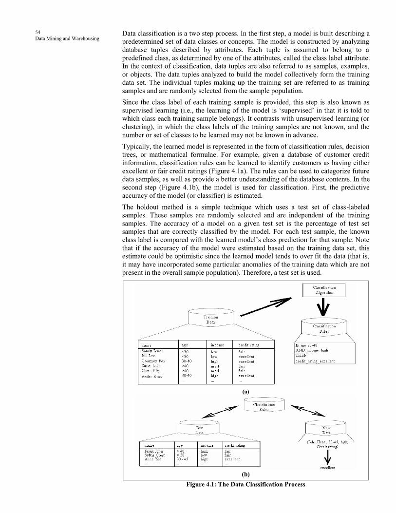
54


Data classification is a two step process. In the first step, a model is built describing a

predetermined set of data classes or concepts. The model is constructed by analyzing

database tuples described by attributes. Each tuple is assumed to belong to a

predefined class, as determined by one of the attributes, called the class label attribute.

In the context of classification, data tuples are also referred to as samples, examples,

or objects. The data tuples analyzed to build the model collectively form the training

data set. The individual tuples making up the training set are referred to as training

samples and are randomly selected from the sample population.

Since the class label of each training sample is provided, this step is also known as

supervised learning (i.e., the learning of the model is ‘supervised’ in that it is told to

which class each training sample belongs). It contrasts with unsupervised learning (or

clustering), in which the class labels of the training samples are not known, and the

number or set of classes to be learned may not be known in advance.

Typically, the learned model is represented in the form of classification rules, decision

trees, or mathematical formulae. For example, given a database of customer credit

information, classification rules can be learned to identify customers as having either

excellent or fair credit ratings (Figure 4.1a). The rules can be used to categorize future

data samples, as well as provide a better understanding of the database contents. In the

second step (Figure 4.1b), the model is used for classification. First, the predictive

accuracy of the model (or classifier) is estimated.

The holdout method is a simple technique which uses a test set of class-labeled

samples. These samples are randomly selected and are independent of the training

samples. The accuracy of a model on a given test set is the percentage of test set

samples that are correctly classified by the model. For each test sample, the known

class label is compared with the learned model’s class prediction for that sample. Note

that if the accuracy of the model were estimated based on the training data set, this

estimate could be optimistic since the learned model tends to over fit the data (that is,

it may have incorporated some particular anomalies of the training data which are not

present in the overall sample population). Therefore, a test set is used.

(a)

(b)

Figure 4.1: The Data Classification Process

55

Data Mining Classification (a) Learning: Training data are analyzed by a classification algorithm. Here, the class

label attribute is credit_rating, and the learned model or classifier is represented in

the form of classification rule.

(b) Classification: Test data are used to estimate the accuracy of the classification

rules. If the accuracy is considered acceptable, the rules can be applied to the

classification of new data tuples.

4.2 WHAT IS CLASSIFICATION AND PREDICTION?

4.2.1 Classification

Classification is a data mining technique used to predict group membership for data

instances. For example, you may wish to use classification to predict whether the

weather on a particular day will be “sunny”, “rainy” or “cloudy”. Popular

classification techniques include decision trees and neural networks.

In classification, there is a target categorical variable, such as income bracket, which,

for example, could be partitioned into three classes or categories: high income, middle

income, and low income. The data mining model examines a large set of records, each

record containing information on the target variable as well as a set of input

or predictor variables. For example, consider the excerpt from a data set shown in

Table 4.1.

Table 4.1: Excerpt from Data Set for Classifying Income

Suppose that the researcher would like to be able to classify the income brackets of

persons not currently in the database, based on other characteristics associated with

that person, such as age, gender, and occupation. This task is a classification task, very

nicely suited to data mining methods and techniques. The algorithm would proceed

roughly as follows. First, examine the data set containing both the predictor variables

and the (already classified) target variable, income bracket. In this way, the algorithm

(software) “learns about” which combinations of variables are associated with which

income brackets. For example, older females may be associated with the high-income

bracket. This data set is called the training set. Then the algorithm would look at new

records, for which no information about income bracket is available. Based on the

classifications in the training set, the algorithm would assign classifications to the new

records. For example, a 63-year-old female professor might be classified in the high-

income bracket.

Examples of classification tasks in business and research include:

Determining whether a particular credit card transaction is fraudulent

Placing a new student into a particular track with regard to special needs

Assessing whether a mortgage application is a good or bad credit risk

Diagnosing whether a particular disease is present

Determining whether a will was written by the actual deceased, or fraudulently by

someone else

Identifying whether or not certain financial or personal behavior indicates a

possible terrorist threat.

56


Supervised Learning and Unsupervised Learning

The learning of the model is 'supervised' if it is told to which class each training

sample belongs. In contrasts with unsupervised learning (or clustering), in which the

class labels of the training samples are not known, and the number or set of classes to

be learned may not be known in advance.

Typically, the learned model is represented in the form of classification rules, decision

trees, or mathematical formulae.

4.2.2 Prediction

Prediction is similar to classification, except that for prediction, the results lie in the

future. Examples of prediction tasks in business and research include:

Predicting the price of a stock three months into the future

Predicting the percentage increase in traffic deaths next year if the speed limit is

increased

Predicting the winner of this fall’s baseball World Series, based on a comparison

of team statistics

Predicting whether a particular molecule in drug discovery will lead to a

profitable new drug for a pharmaceutical company.

Any of the methods and techniques used for classification may also be used, under

appropriate circumstances, for prediction. These include the traditional statistical

methods of point estimation and confidence interval estimations, simple linear

regression and correlation, and multiple regression.

4.3 ISSUES REGARDING CLASSIFICATION

AND PREDICTION

To prepare the data for classification and prediction, following preprocessing steps

may be applied to the data in order to help improve the accuracy, efficiency, and

scalability of the classification or prediction process.

Data cleaning: This refers to the preprocessing of data in order to remove or

reduce noise (by applying smoothing techniques, for example), and the treatment

of missing values (e.g., by replacing a missing value with the most commonly

occurring value for that attribute, or with the most probable value based on

statistics). Although most classification algorithms have some mechanisms for

handling noisy or missing data, this step can help reduce confusion during

learning.

Relevance analysis: Many of the attributes in the data may be irrelevant to the

classification or prediction task. For example, data recording the day of the week

on which a bank loan application was filled is unlikely to be relevant to the

success of the application. Furthermore, other attributes may be redundant. Hence,

relevance analysis may be performed on the data with the aim of removing any

irrelevant or redundant attributes from the learning process. In machine learning,

this step is known as feature selection. Including such attributes may otherwise

slow down, and possibly mislead, the learning step. Ideally, the time spent on

relevance analysis, when added to the time spent on learning from the resulting

“reduced” feature subset, should be less than the time that would have been spent

on learning from the original set of features. Hence, such analysis can help

improve classification efficiency and scalability.

Data transformation: The data can be generalized to higher-level concepts.

Concept hierarchies may be used for this purpose. This is particularly useful for

57

Data Mining Classification continuous-valued attributes. For example, numeric values for the attribute

income may be generalized to discrete ranges such as low, medium, and high.

Similarly, nominal-valued attributes, like street, can be generalized to higher-level

concepts, like city. Since generalization compresses the original training data,

fewer input/output operations may be involved during learning. The data may also

be normalized, particularly when neural networks or methods involving distance

measurements are used in the learning step. Normalization involves scaling all

values for a given attribute so that they fall within a small specified range, such as

-1.0 to 1.0, or 0 to 1.0. In methods which use distance measurements, for example,

this would prevent attributes with initially large ranges (like, say income) from

outweighing attributes with initially smaller ranges (such as binary attributes).


Define the following:

1. Speed

…………………………………….………………………………………..

…………………………………….………………………………………..

2. Scalability

…………………………………….………………………………………..

…………………………………….………………………………………..

3. Interpretability

…………………………………….………………………………………..

…………………………………….………………………………………..

4.4 STATISTICAL BASED ALGORITHMS

Bayesian classifiers are statistical classifiers. They can predict class membership

probabilities, such as the probability that a given sample belongs to a particular class.

Bayesian classification is based on Bayes theorem. Bayesian classifiers exhibited high

accuracy and speed when applied to large databases.

Studies comparing classification algorithms have found a simple Bayesian classifier

known as the Naive Bayesian classifier to be comparable in performance with

decision tree and neural network classifiers. Naive Bayesian classifiers assume that

the effect of an attribute value on a given class is independent of the values of the

other attributes. This assumption is called class conditional independence. It is made

to simplify the computations involved, and in this sense, is considered "naive".

Bayesian belief networks are graphical models, which unlike naive Bayesian

classifiers, allow the representation of dependencies among subsets of attributes.

Apply Bayes Rule: c is the class, v observed attribute values:

( | ) ( )( | )

( )

P v c P cP c v

P v=

If we assume k possible disjoint diagnoses, c1, …, cK

( ( | )( | )

( )

k k

k

P c P v cP c v

P v=

P(v) may not be known, but total probability of diagnoses is 1

58


P(v) (the evidence): ( ( | )

1( )

k k

k

P c P v c

P v=

P(v) = k P(ck) P(v|ck)

Need to know P(ck), P(v|ck) for all k

Bayes Rules: likelihood × prior

posterior = evidence

MAP vs ML

Rather than computing full posterior, can simplify computation if interested in

classification:

1. ML (Maximum Likelihood) Hypothesis

assume all hypotheses equiprobable a priori – simply maximize data likelihood:

MLc C

c = arg max P(v|c)Î

2. MAP (Maximum A Posteriori) Class Hypothesis

MAPc C

c = arg max P(c|v)Î

c c

P(vc/P(c))arg max

P(v)Î

can ignore denominator because same for all c

Bayes Theorem:

Bayes' theorem relates the conditional and marginal probabilities of events A and B,

where B has a non-vanishing probability:

P(B|A)P(A)P(A|B) = .

P(B)

Each term in Bayes' theorem has a conventional name:

P(A) is the prior probability or marginal probability of A. It is "prior" in the sense

that it does not take into account any information about B.

P(A|B) is the conditional probability of A, given B. It is also called the posterior

probability because it is derived from or depends upon the specified value of B.

P(B|A) is the conditional probability of B given A.

P(B) is the prior or marginal probability of B, and acts as a normalizing constant.

Intuitively, Bayes' theorem in this form describes the way in which one's beliefs about

observing ‘A’ are updated by having observed ‘B’.

Bayes Theorem: Example: Use training examples to estimate class-conditional

probability density functions for white-blood cell count (W)

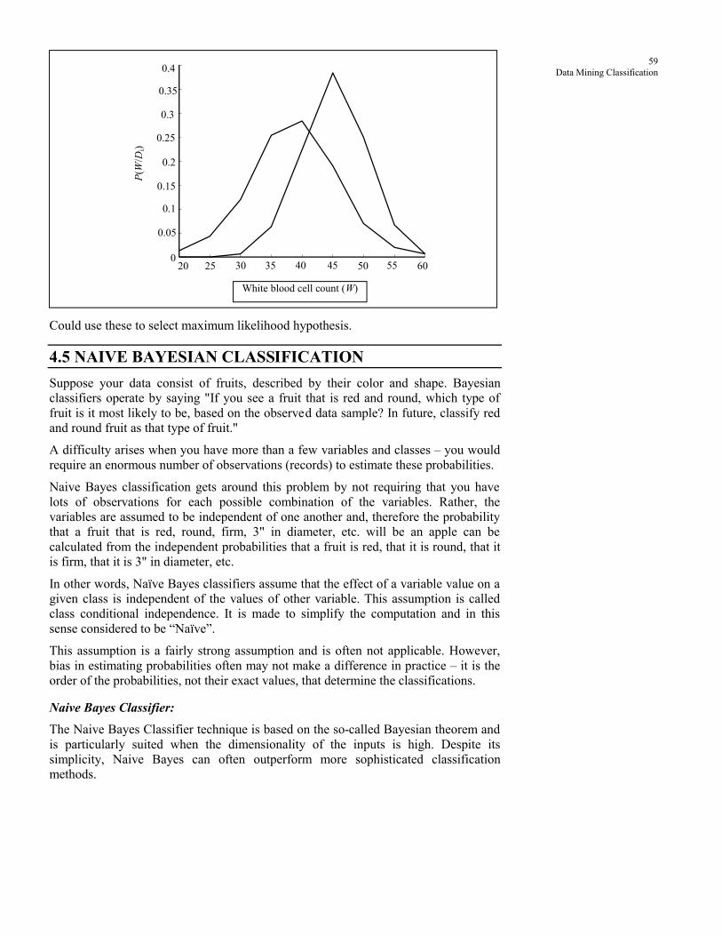
59


Could use these to select maximum likelihood hypothesis.

4.5 NAIVE BAYESIAN CLASSIFICATION

Suppose your data consist of fruits, described by their color and shape. Bayesian

classifiers operate by saying "If you see a fruit that is red and round, which type of

fruit is it most likely to be, based on the observed data sample? In future, classify red

and round fruit as that type of fruit."

A difficulty arises when you have more than a few variables and classes – you would

require an enormous number of observations (records) to estimate these probabilities.

Naive Bayes classification gets around this problem by not requiring that you have

lots of observations for each possible combination of the variables. Rather, the

variables are assumed to be independent of one another and, therefore the probability

that a fruit that is red, round, firm, 3" in diameter, etc. will be an apple can be

calculated from the independent probabilities that a fruit is red, that it is round, that it

is firm, that it is 3" in diameter, etc.

In other words, Naïve Bayes classifiers assume that the effect of a variable value on a

given class is independent of the values of other variable. This assumption is called

class conditional independence. It is made to simplify the computation and in this

sense considered to be “Naïve”.

This assumption is a fairly strong assumption and is often not applicable. However,

bias in estimating probabilities often may not make a difference in practice – it is the

order of the probabilities, not their exact values, that determine the classifications.

Naive Bayes Classifier:

The Naive Bayes Classifier technique is based on the so-called Bayesian theorem and

is particularly suited when the dimensionality of the inputs is high. Despite its

simplicity, Naive Bayes can often outperform more sophisticated classification

methods.

0.4

0.35

0.3

0.25

0.2

0.15

0.1

0.05

0 20 25 30 35 40 45 50 55 60

P(W

/Di)

White blood cell count (W)

60


To demonstrate the concept of Naïve Bayes Classification, consider the example

displayed in the illustration above. As indicated, the objects can be classified as either

GREY or BLACK. Our task is to classify new cases as they arrive, i.e., decide to

which class label they belong, based on the currently exiting objects.

Since there are twice as many GREY objects as BLACK, it is reasonable to believe

that a new case (which hasn't been observed yet) is twice as likely to have

membership GREY rather than BLACK. In the Bayesian analysis, this belief is known

as the prior probability. Prior probabilities are based on previous experience, in this

case the percentage of GREY and BLACK objects, and often used to predict

outcomes before they actually happen.

Thus, we can write:

Number of Grey objectsPrior probability for Grey

Total number of objectsµ

Number of Black objectsPrior probability for Black

Total number of objectsµ

Since there is a total of 60 objects, 40 of which are GREY and 20 BLACK, our prior

probabilities for class membership are:

Prior probability for Grey µ 40

60

Prior probability for Black µ 20

60

Having formulated our prior probability, we are now ready to classify a new object

(WHITE circle). Since the objects are well clustered, it is reasonable to assume that

the more GREY (or BLACK) objects in the vicinity of X, the more likely that the new

cases belong to that particular color. To measure this likelihood, we draw a circle

around X which encompasses a number (to be chosen a priori) of points irrespective

of their class labels. Then we calculate the number of points in the circle belonging to

each class label. From this we calculate the likelihood:

Number of Grey in the vicinity of XLikelihood of X given Grey

Total number of Grey casesµ

Number of Black in the vicinity of XLikelihood of X given Black

Total number of Black casesµ

61

Data Mining Classification From the illustration above, it is clear that Likelihood of X given GREY is smaller

than Likelihood of X given BLACK, since the circle encompasses 1 GREY object and

3 BLACK ones. Thus:

Probability of X given Grey µ 1

40

Probability of X given Black µ 3

20

Although the prior probabilities indicate that X may belong to GREY (given that there

are twice as many GREY compared to BLACK) the likelihood indicates otherwise;

that the class membership of X is BLACK (given that there are more BLACK objects

in the vicinity of X than GREY). In the Bayesian analysis, the final classification is

produced by combining both sources of information, i.e., the prior and the likelihood,

to form a posterior probability using the so-called Bayes' rule (named after Rev.

Thomas Bayes 1702-1761).

Posterior probability of X being Grey µ

Prior probability of Grey × Likelihood of X given Grey

4 1 1

6 40 60= ´ =

Posterior probability of X being Black µ

Prior probability of Black × Likelihood of X given Black

2 3 1

6 20 20= ´ =

Finally, we classify X as BLACK since its class membership achieves the largest

posterior probability.

How Effective are Bayesian Classifiers?

In theory, Bayesian classifiers have the minimum error rate in comparison to all other

classifiers. However, in practice this is not always the case owing to inaccuracies in

the assumptions made for its use, such as class conditional independence, and the lack

of available probability data. However, various empirical studies of this classifier in

comparison to decision tree and neural network classifiers have found it to be

comparable in some domains.

Bayesian classifiers are also useful in that they provide a theoretical justification for

other classifiers which do not explicitly use Bayes theorem. For example, under

certain assumptions, it can be shown that many neural network and curve fitting

algorithms output the maximum posteriori hypothesis, as does the naive Bayesian

classifier.


Fill in the blanks:

1. Bayesian classifiers are ……………….. classifiers.

2. Bayesian classification is based on ……………….. theorem.

3. ……………….. classifiers assume that the effect of an attribute value on

a given class is independent of the values of the other attributes.

4. Bayesian belief networks are ……………….. models.

5. In theory, ……………….. classifiers have the minimum error rate in

comparison to all other classifiers.

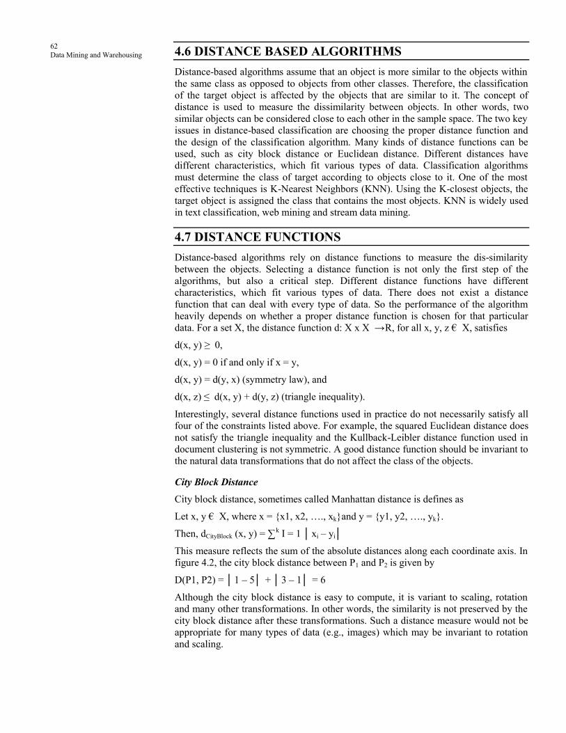
62


4.6 DISTANCE BASED ALGORITHMS

Distance-based algorithms assume that an object is more similar to the objects within

the same class as opposed to objects from other classes. Therefore, the classification

of the target object is affected by the objects that are similar to it. The concept of

distance is used to measure the dissimilarity between objects. In other words, two

similar objects can be considered close to each other in the sample space. The two key

issues in distance-based classification are choosing the proper distance function and

the design of the classification algorithm. Many kinds of distance functions can be

used, such as city block distance or Euclidean distance. Different distances have

different characteristics, which fit various types of data. Classification algorithms

must determine the class of target according to objects close to it. One of the most

effective techniques is K-Nearest Neighbors (KNN). Using the K-closest objects, the

target object is assigned the class that contains the most objects. KNN is widely used

in text classification, web mining and stream data mining.

4.7 DISTANCE FUNCTIONS

Distance-based algorithms rely on distance functions to measure the dis-similarity

between the objects. Selecting a distance function is not only the first step of the

algorithms, but also a critical step. Different distance functions have different

characteristics, which fit various types of data. There does not exist a distance

function that can deal with every type of data. So the performance of the algorithm

heavily depends on whether a proper distance function is chosen for that particular

data. For a set X, the distance function d: X x X → R, for all x, y, z € X, satisfies

d(x, y) ≥ 0,

d(x, y) = 0 if and only if x = y,

d(x, y) = d(y, x) (symmetry law), and

d(x, z) ≤ d(x, y) + d(y, z) (triangle inequality).

Interestingly, several distance functions used in practice do not necessarily satisfy all

four of the constraints listed above. For example, the squared Euclidean distance does

not satisfy the triangle inequality and the Kullback-Leibler distance function used in

document clustering is not symmetric. A good distance function should be invariant to

the natural data transformations that do not affect the class of the objects.

City Block Distance

City block distance, sometimes called Manhattan distance is defines as

Let x, y € X, where x = x1, x2, …., xkand y = y1, y2, …., yk.

Then, dCityBlock (x, y) = ∑k I = 1 xi – yi

This measure reflects the sum of the absolute distances along each coordinate axis. In

figure 4.2, the city block distance between P1 and P2 is given by

D(P1, P2) = 1 – 5 + 3 – 1 = 6

Although the city block distance is easy to compute, it is variant to scaling, rotation

and many other transformations. In other words, the similarity is not preserved by the

city block distance after these transformations. Such a distance measure would not be

appropriate for many types of data (e.g., images) which may be invariant to rotation

and scaling.

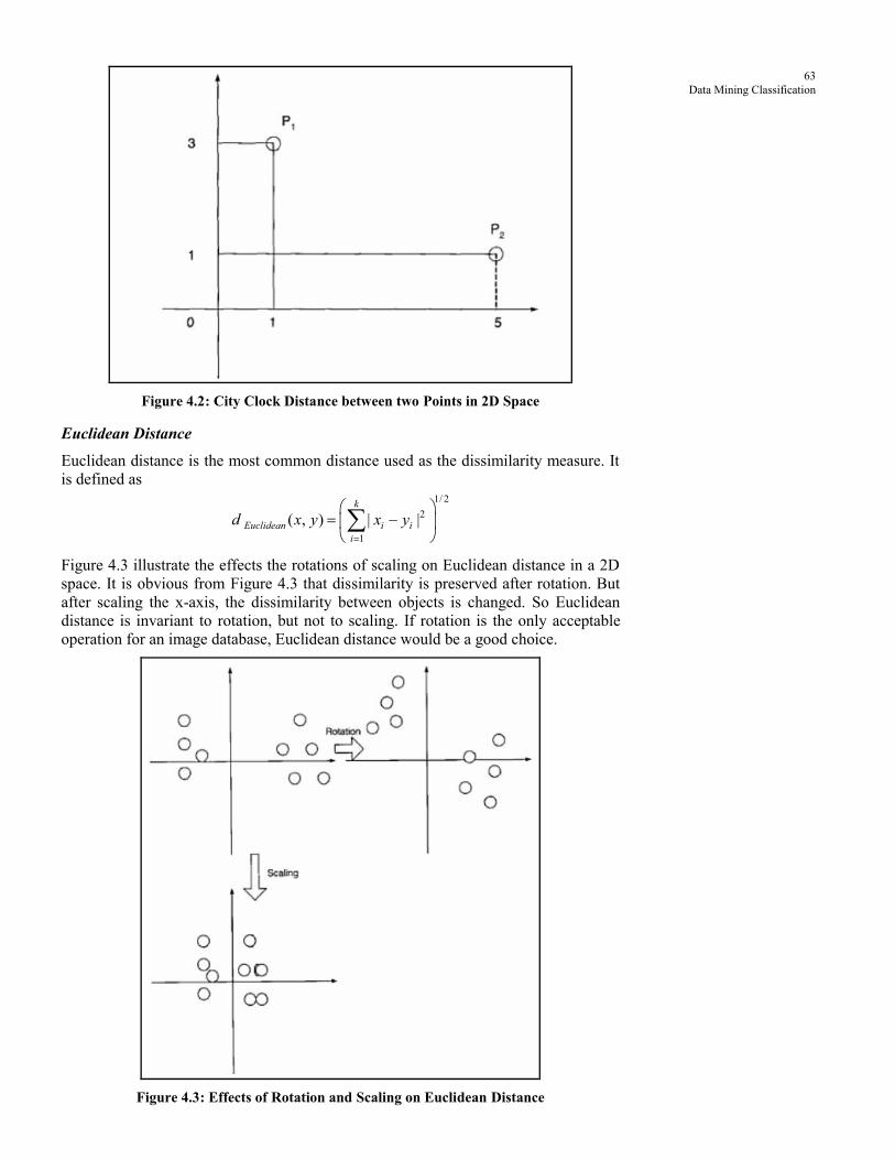
63


Figure 4.2: City Clock Distance between two Points in 2D Space

Euclidean Distance

Euclidean distance is the most common distance used as the dissimilarity measure. It

is defined as 1/ 2

2

1

( , ) | – |k

Euclidean i i

i

d x y x y=

=

Figure 4.3 illustrate the effects the rotations of scaling on Euclidean distance in a 2D

space. It is obvious from Figure 4.3 that dissimilarity is preserved after rotation. But

after scaling the x-axis, the dissimilarity between objects is changed. So Euclidean

distance is invariant to rotation, but not to scaling. If rotation is the only acceptable

operation for an image database, Euclidean distance would be a good choice.

Figure 4.3: Effects of Rotation and Scaling on Euclidean Distance

64


Other Distances

There are also many other distances that can be used for different data. Edit distance

fits sequence and text data. The Tanimoto distance is suitable for data with binary-

valued features.

Actually, data normalization is one way to overcome the limitation of the distance

functions. Functions. For example, normalizing the data to the same scale can

overcome the scaling problem of Euclidean distance, however, normalization may

lead to information loss and lower classification accuracy.

4.8 CLASSIFICATION BY DECISION TREE

A decision tree is a flow-chart-like tree structure, where each internal node denotes a

test on an attribute, each branch represents an outcome of the test, and leaf nodes

represent classes or class distributions. The topmost node in a tree is the root node.

For example, to decide whether play golf or not, let us consider the following decision

tree (see Figure 4.4)

Figure 4.4: Decision Tree for the Golf Example

In order to determine the decision (classification) for a given set of weather conditions

from the decision tree, first look at the value of Outlook. There are three possibilities.

If the value of Outlook is sunny, next consider the value of Humidity. If the value

is less than or equal to 75 the decision is play. Otherwise the decision is don’t

play.

If the value of Outlook is overcast, the decision is play.

If the value of Outlook is rain, next consider the value of Windy. If the value is

true the decision is don’t play, otherwise the decision is play.

Decision Trees are useful for predicting exact outcomes. Applying the decision trees

algorithm to a training dataset results in the formation of a tree that allows the user to

map a path to a successful outcome. At every node along the tree, the user answers a

question (or makes a “decision”), such as “play” or “don’t play”.

The decision trees algorithm would be useful for a bank that wants to ascertain the

characteristics of good customers. In this case, the predicted outcome is whether or

not the applicant represents a bad credit risk. The outcome of a decision tree may be a

Yes/No result (applicant is/is not a bad credit risk) or a list of numeric values, with

each value assigned a probability.

The training dataset consists of the historical data collected from past loans. Attributes

that affect credit risk might include the customer's educational level, the number of

kids the customer has, or the total household income. Each split on the tree represents

a decision that influences the final predicted variable. For example, a customer who

graduated from high school may be more likely to pay back the loan. The variable

used in the first split is considered the most significant factor. So if educational level

is in the first split, it is the factor that most influences credit risk.

65

Data Mining Classification Decision trees have been used in many application areas ranging from medicine to

game theory and business. Decision trees are the basis of several commercial rule

induction systems.

Basic Algorithm for Learning Decision Trees

Algorithm: Generate a decision tree from the given training data.

Input: The training samples, samples, represented by discrete-valued attributes; the

set of candidate attributes, attribute-list.

Output: A decision tree.

Method

create a node N;

if samples are all of the same class, C then

return N as a leaf node labeled with the class C

if attribute-list is empty then

return N as a leaf node labeled with the most common class in samples; //

majority voting

select test-attribute, the attribute among attribute-list with the highest information

gain

label node N with test-attribute

for each known value ai of test-attribute // partition the samples

grow a branch from node N for the condition test-attribute = ai

let si be the set of samples in samples for which test-attribute = ai; // a partition

if si is empty then

attach a leaf labeled with the most common class in samples

else attach the node returned by Generate decision tree (si, attribute-list-test-

attribute).

Decision Tree Induction

The automatic generation of decision rules from examples is known as rule induction

or automatic rule induction.

Generating decision rules in the implicit form of a decision tree are also often called

rule induction, but the terms tree induction or decision tree inductions are sometimes

preferred.

The basic algorithm for decision tree induction is a greedy algorithm, which

constructs decision trees in a top-down recursive divide-and-conquer manner. The

Basic algorithm for learning decision trees, is a version of ID3, a well-known decision

tree induction algorithm.

The basic strategy is as follows:

The tree starts as a single node representing the training samples (step 1).

If the samples are all of the same class, then the node becomes a leaf and is

labeled with that class (steps 2 and 3).

Otherwise, the algorithm uses an entropy-based measure known as information

gain as a heuristic for selecting the attribute that will best separate the samples

into individual classes (step 6). This attribute becomes the "test" or "decision"

66


attribute at the node (step 7). In this version of the algorithm, all attributes are

categorical, i.e., discrete-valued. Continuous-valued attributes must be discretized.

A branch is created for each known value of the test attribute, and the samples are

partitioned accordingly (steps 8-10).

The algorithm uses the same process recursively to form a decision tree for the

samples at each partition. Once an attribute has occurred at a node, it need not be

considered in any of the node's descendents (step 13).

The recursive partitioning stops only when any one of the following conditions is

true:

All samples for a given node belong to the same class (steps 2 and 3), or

There are no remaining attributes on which the samples may be further

partitioned (step 4). In this case, majority voting is employed (step 5). This

involves converting the given node into a leaf and labeling it with the class in

majority among samples. Alternatively, the class distribution of the node

samples may be stored; or

There are no samples for the branch test-attribute = at (step 11). In this case, a

leaf is created with the majority class in samples (step 12).

Decision tree induction algorithms have been used for classification in a wide range of

application domains. Such systems do not use domain knowledge. The learning and

classification steps of decision tree induction are generally fast. Classification

accuracy is typically high for data where the mapping of classes consists of long and

thin regions in concept space.

Attribute Selection Measure

The information gain measure is used to select the test attribute at each node in the

tree. Such a measure is also referred to as an attribute selection measure. The attribute

with the highest information gain is chosen as the test attribute for the current node.

This attribute minimizes the information needed to classify the samples in the

resulting partitions and reflects the least randomness or "impurity" in these partitions.

Such an information-theoretic approach minimizes the expected number of tests

needed to classify an object and guarantees that a simple (but not necessarily the

simplest) tree is found.

Let S be a set consisting of s data samples. Suppose the class label attribute has m

distinct values defining m distinct classes, d (for i = 1,..., m). Let s, be the number of

samples of S in class d. The expected information needed to classify a given sample is

given by:

I(s1, s2 …, sm) = 2

1

– log ( )m

i i

i

p p=

where p, is the probability than an arbitrary sample belongs to class d and is estimated

by Si/s. Note that a log function to the base 2 is used since the information is encoded

in bits.

Attribute A can be used to partition S into v subsets, S1, S2, ….. , SV, where Sj

contains those samples in S that have value aj of A. If A were selected as the test

attribute (i.e., best attribute for splitting), then these subsets would correspond to the

branches grown from the node containing the set S. Let sj be the number of samples of

class d in a subset Sj. The entropy, or expected information based on the partitioning

into subsets by A is given by:

1

1

1

...( ) ( ... ).

vj mj

j mj

i

s sE A I s s

s=

=

67

Data Mining Classification The term 1

1

...v j mj

i

s s

s=

acts as the weight of the j

th subset and is the number of

samples in the subset (i.e., having value aj of A) divided by the total number of

samples in S. The smaller the entropy value is, the greater the purity of the subset

partitions. The encoding information that would be gained by branching on A is

Gain(A) = I(8l, s2, . . . , sm) - E(A).

In other words, Gain(A) is the expected reduction in entropy caused by knowing the

value of attribute A.

The algorithm computes the information gain of each attribute. The attribute with the

highest information gain is chosen as the test attribute for the given set S. A node is

created and labeled with the attribute, branches are created for each value of the

attribute, and the samples are partitioned accordingly.

Tree Pruning

After building a decision tree a tree pruning step can be performed to reduce the size

of the decision tree. Decision trees that are too large are susceptible to a phenomenon

called as overfitting. Pruning helps by trimming the branches that reflects anomalies

in the training data due to noise or outliers and helps the initial tree in a way that

improves the generalization capability of the tree. Such methods typically use

statistical measures to remove the least reliable branches, generally resulting in faster

classification and an improvement in the ability of the tree to correctly classify

independent test data.

There are two common approaches to tree pruning.

(a) Pre-pruning Approach: In the pre-pruning approach, a tree is "pruned" by halting

its construction early (e.g., by deciding not to further split or partition the subset

of training samples at a given node). Upon halting, the node becomes a leaf. The

leaf may hold the most frequent class among the subset samples, or the probability

distribution of those samples.

When constructing a tree, measures such as statistical significance, x2,

information gain, etc., can be used to assess the goodness of a split. If partitioning

the samples at a node would result in a split that falls below a pre-specified

threshold, then further partitioning of the given subset is halted. There are

difficulties, however, in choosing an appropriate threshold. High thresholds could

result in oversimplified trees, while low thresholds could result in very little

simplification.

(b) Post-pruning Approach: The post-pruning approach removes branches from a

"fully grown" tree. A tree node is pruned by removing its branches.

The cost complexity pruning algorithm is an example of the post-pruning

approach. The pruned node becomes a leaf and is labeled by the most frequent

class among its former branches. For each non-leaf node in the tree, the algorithm

calculates the expected error rate that would occur if the subtree at that node were

pruned. Next, the expected error rate occurring if the node were not pruned is

calculated using the error rates for each branch, combined by weighting according

to the proportion of observations along each branch. If pruning the node leads to a

greater expected error rate, then the subtree is kept. Otherwise, it is pruned. After

generating a set of progressively pruned trees, an independent test set is used to

estimate the accuracy of each tree. The decision tree that minimizes the expected

error rate is preferred.

Example

A company is trying to decide whether to bid for a certain contract or not. They

estimate that merely preparing the bid will cost £10,000. If their company bid then

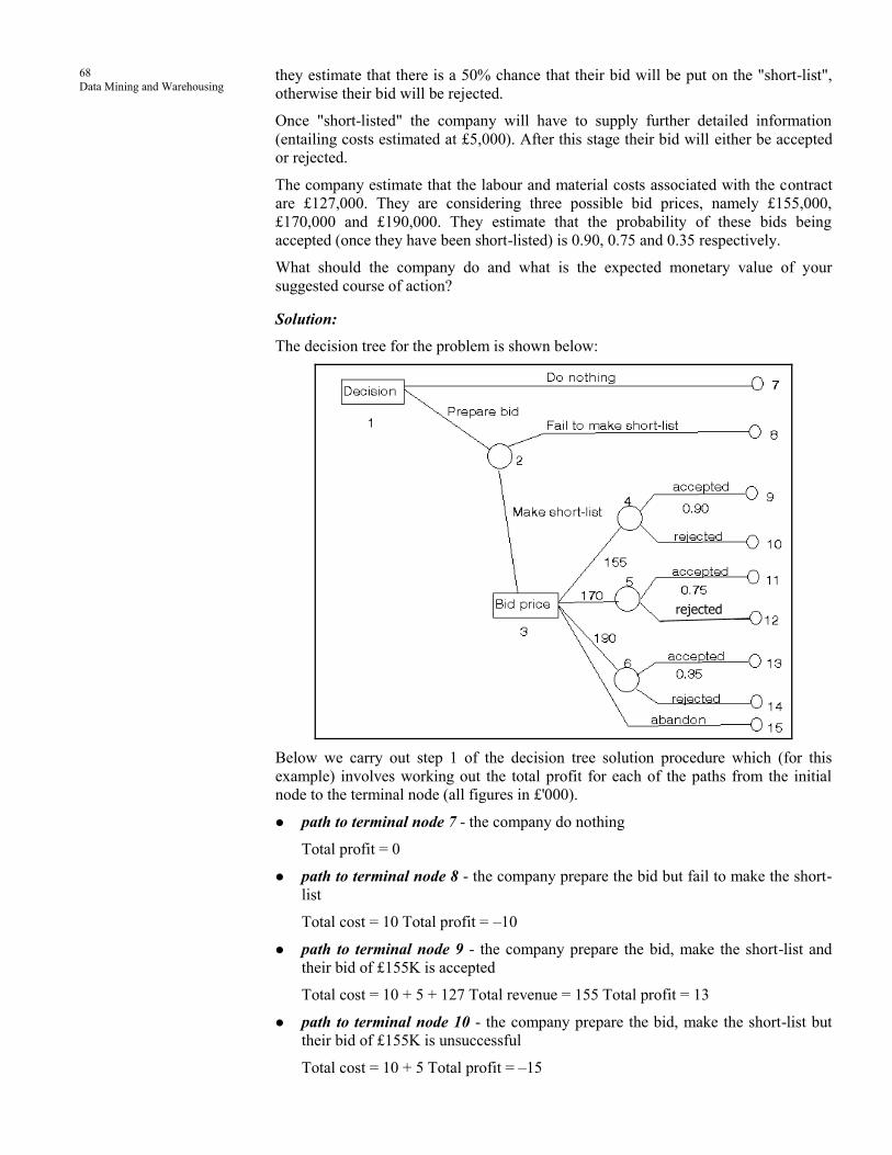
68


they estimate that there is a 50% chance that their bid will be put on the "short-list",

otherwise their bid will be rejected.

Once "short-listed" the company will have to supply further detailed information

(entailing costs estimated at £5,000). After this stage their bid will either be accepted

or rejected.

The company estimate that the labour and material costs associated with the contract

are £127,000. They are considering three possible bid prices, namely £155,000,

£170,000 and £190,000. They estimate that the probability of these bids being

accepted (once they have been short-listed) is 0.90, 0.75 and 0.35 respectively.

What should the company do and what is the expected monetary value of your

suggested course of action?

Solution:

The decision tree for the problem is shown below:

Below we carry out step 1 of the decision tree solution procedure which (for this

example) involves working out the total profit for each of the paths from the initial

node to the terminal node (all figures in £'000).

path to terminal node 7 - the company do nothing

Total profit = 0

path to terminal node 8 - the company prepare the bid but fail to make the short-

list

Total cost = 10 Total profit = –10

path to terminal node 9 - the company prepare the bid, make the short-list and

their bid of £155K is accepted

Total cost = 10 + 5 + 127 Total revenue = 155 Total profit = 13

path to terminal node 10 - the company prepare the bid, make the short-list but

their bid of £155K is unsuccessful

Total cost = 10 + 5 Total profit = –15

rejected

69

Data Mining Classification path to terminal node 11 - the company prepare the bid, make the short-list and






path to terminal node 13 - the company prepare the bid, make the short-list and






path to terminal node 15 - the company prepare the bid and make the short-list

and then decide to abandon bidding (an implicit option available to the company)


Hence we can arrive at the table below indicating for each branch the total profit

involved in that branch from the initial node to the terminal node.

Terminal node Total profit £

7 0

8 –10

9 13

10 –15

11 28

12 –15

13 48

14 –15

15 –15

We can now carry out the second step of the decision tree solution procedure where

we work from the right-hand side of the diagram back to the left-hand side.


Fill in the blanks:

1. …………………… is a data mining technique used to predict group

membership for data instances.

2. The learning of the model is …………………… if it is told to which

class each training sample belongs.

3. …………………… refers to the ability of the model to correctly predict

the class label of new or previously unseen data.

4. A …………………… is a flow-chart-like tree structure.

5. The …………………… measure is used to select the test attribute at each

node in the tree.

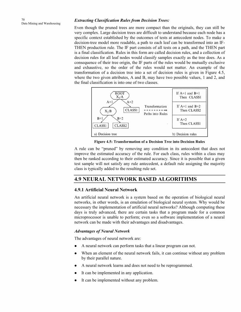
70


Extracting Classification Rules from Decision Trees:

Even though the pruned trees are more compact than the originals, they can still be

very complex. Large decision trees are difficult to understand because each node has a

specific context established by the outcomes of tests at antecedent nodes. To make a

decision-tree model more readable, a path to each leaf can be transformed into an IF-

THEN production rule. The IF part consists of all tests on a path, and the THEN part

is a final classification. Rules in this form are called decision rules, and a collection of

decision rules for all leaf nodes would classify samples exactly as the tree does. As a

consequence of their tree origin, the IF parts of the rules would be mutually exclusive

and exhaustive, so the order of the rules would not matter. An example of the

transformation of a decision tree into a set of decision rules is given in Figure 4.5,

where the two given attributes, A and B, may have two possible values, 1 and 2, and

the final classification is into one of two classes.

Figure 4.5: Transformation of a Decision Tree into Decision Rules

A rule can be “pruned” by removing any condition in its antecedent that does not

improve the estimated accuracy of the rule. For each class, rules within a class may

then be ranked according to their estimated accuracy. Since it is possible that a given

test sample will not satisfy any rule antecedent, a default rule assigning the majority

class is typically added to the resulting rule set.

4.9 NEURAL NETWORK BASED ALGORITHMS

4.9.1 Artificial Neural Network

An artificial neural network is a system based on the operation of biological neural

networks, in other words, is an emulation of biological neural system. Why would be

necessary the implementation of artificial neural networks? Although computing these

days is truly advanced, there are certain tasks that a program made for a common

microprocessor is unable to perform; even so a software implementation of a neural

network can be made with their advantages and disadvantages.

Advantages of Neural Network

The advantages of neural network are:

A neural network can perform tasks that a linear program can not.

When an element of the neural network fails, it can continue without any problem

by their parallel nature.

A neural network learns and does not need to be reprogrammed.

It can be implemented in any application.

It can be implemented without any problem.

71

Data Mining Classification Disadvantages of Neural Network

The disadvantages of neural network are:

The neural network needs training to operate.

The architecture of a neural network is different from the architecture of

microprocessors therefore needs to be emulated.

Requires high processing time for large neural networks.

Another aspect of the artificial neural networks is that there are different architectures,

which consequently requires different types of algorithms, but despite to be an

apparently complex system, a neural network is relatively simple.

Artificial Neural Networks (ANN) are among the newest signal-processing

technologies in the engineer's toolbox. The field is highly interdisciplinary, but our

approach will restrict the view to the engineering perspective. In engineering, neural

networks serve two important functions: as pattern classifiers and as non-linear

adaptive filters. We will provide a brief overview of the theory, learning rules, and

applications of the most important neural network models. Definitions and style of

computation an Artificial Neural Network is an adaptive, most often nonlinear system

that learns to perform a function (an input/output map) from data. Adaptive means

that the system parameters are changed during operation, normally called the training

phase. After the training phase the Artificial Neural Network parameters are fixed and

the system is deployed to solve the problem at hand (the testing phase). The Artificial

Neural Network is built with a systematic step-by-step procedure to optimize a

performance criterion or to follow some implicit internal constraint, which is

commonly referred to as the learning rule. The input/output training data are

fundamental in neural network technology, because they convey the necessary

information to "discover" the optimal operating point. The nonlinear nature of the

neural network processing elements (PEs) provides the system with lots of flexibility

to achieve practically any desired input/output map, i.e., some Artificial Neural

Networks are universal mappers. There is a style in neural computation that is worth

describing.

Figure 4.6: The Style of Neutral Computation

An input is presented to the neural network and a corresponding desired or target

response set at the output (when this is the case the training is called supervised). An

error is composed from the difference between the desired response and the system

output. This error information is fed back to the system and adjusts the system

parameters in a systematic fashion (the learning rule). The process is repeated until the

performance is acceptable. It is clear from this description that the performance hinges

heavily on the data. If one does not have data that cover a significant portion of the

operating conditions or if they are noisy, then neural network technology is probably

not the right solution. On the other hand, if there is plenty of data and the problem is

poorly understood to derive an approximate model, then neural network technology is

a good choice. This operating procedure should be contrasted with the traditional

72


engineering design, made of exhaustive subsystem specifications and

intercommunication protocols. In artificial neural networks, the designer chooses the

network topology, the performance function, the learning rule, and the criterion to

stop the training phase, but the system automatically adjusts the parameters. So, it is

difficult to bring a priori information into the design, and when the system does not

work properly it is also hard to incrementally refine the solution. But ANN-based

solutions are extremely efficient in terms of development time and resources, and in

many difficult problems artificial neural networks provide performance that is

difficult to match with other technologies. Denker 10 years ago said that "artificial

neural networks are the second best way to implement a solution" motivated by the

simplicity of their design and because of their universality, only shadowed by the

traditional design obtained by studying the physics of the problem. At present,

artificial neural networks are emerging as the technology of choice for many

applications, such as pattern recognition, prediction, system identification, and

control.

4.9.2 Biological Model

Artificial neural networks emerged after the introduction of simplified neurons by

McCulloch and Pitts in 1943 (McCulloch & Pitts, 1943). These neurons were

presented as models of biological neurons and as conceptual components for circuits

that could perform computational tasks. The basic model of the neuron is founded

upon the functionality of a biological neuron. "Neurons are the basic signaling units of

the nervous system" and "each neuron is a discrete cell whose several processes arise

from its cell body".

Figure 4.7

The neuron has four main regions to its structure. The cell body, or soma, has two

offshoots from it, the dendrites, and the axon, which end in presynaptic terminals. The

cell body is the heart of the cell, containing the nucleus and maintaining protein

synthesis. A neuron may have many dendrites, which branch out in a treelike

structure, and receive signals from other neurons. A neuron usually only has one axon

which grows out from a part of the cell body called the axon hillock. The axon

conducts electric signals generated at the axon hillock down its length. These electric

signals are called action potentials. The other end of the axon may split into several

branches, which end in a presynaptic terminal. Action potentials are the electric

signals that neurons use to convey information to the brain. All these signals are

identical. Therefore, the brain determines what type of information is being received

based on the path that the signal took. The brain analyzes the patterns of signals being

sent and from that information it can interpret the type of information being received.

Myelin is the fatty tissue that surrounds and insulates the axon. Often short axons do

not need this insulation. There are uninsulated parts of the axon. These areas are

called Nodes of Ranvier. At these nodes, the signal traveling down the axon is

regenerated. This ensures that the signal traveling down the axon travels fast and

remains constant (i.e. very short propagation delay and no weakening of the signal).

The synapse is the area of contact between two neurons. The neurons do not actually

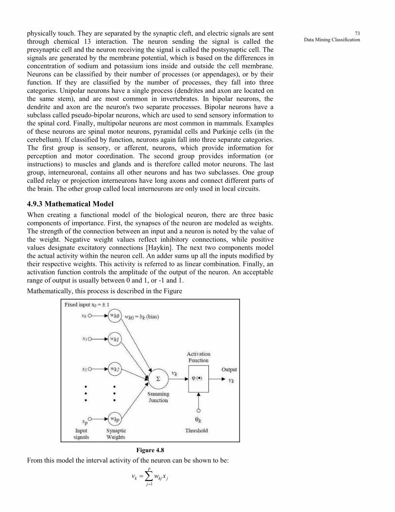
73

Data Mining Classification physically touch. They are separated by the synaptic cleft, and electric signals are sent

through chemical 13 interaction. The neuron sending the signal is called the

presynaptic cell and the neuron receiving the signal is called the postsynaptic cell. The

signals are generated by the membrane potential, which is based on the differences in

concentration of sodium and potassium ions inside and outside the cell membrane.

Neurons can be classified by their number of processes (or appendages), or by their

function. If they are classified by the number of processes, they fall into three

categories. Unipolar neurons have a single process (dendrites and axon are located on

the same stem), and are most common in invertebrates. In bipolar neurons, the

dendrite and axon are the neuron's two separate processes. Bipolar neurons have a

subclass called pseudo-bipolar neurons, which are used to send sensory information to

the spinal cord. Finally, multipolar neurons are most common in mammals. Examples

of these neurons are spinal motor neurons, pyramidal cells and Purkinje cells (in the

cerebellum). If classified by function, neurons again fall into three separate categories.

The first group is sensory, or afferent, neurons, which provide information for

perception and motor coordination. The second group provides information (or

instructions) to muscles and glands and is therefore called motor neurons. The last

group, interneuronal, contains all other neurons and has two subclasses. One group

called relay or projection interneurons have long axons and connect different parts of

the brain. The other group called local interneurons are only used in local circuits.

4.9.3 Mathematical Model

When creating a functional model of the biological neuron, there are three basic

components of importance. First, the synapses of the neuron are modeled as weights.

The strength of the connection between an input and a neuron is noted by the value of

the weight. Negative weight values reflect inhibitory connections, while positive

values designate excitatory connections [Haykin]. The next two components model

the actual activity within the neuron cell. An adder sums up all the inputs modified by

their respective weights. This activity is referred to as linear combination. Finally, an

activation function controls the amplitude of the output of the neuron. An acceptable

range of output is usually between 0 and 1, or -1 and 1.

Mathematically, this process is described in the Figure

Figure 4.8

From this model the interval activity of the neuron can be shown to be:

1

p

k kj j

j

v w x=

=

74


The output of the neuron, yk, would therefore be the outcome of some activation

function on the value of vk.

Activation functions

As mentioned previously, the activation function acts as a squashing function, such

that the output of a neuron in a neural network is between certain values (usually 0

and 1, or -1 and 1). In general, there are three types of activation functions, denoted by

Φ(.). First, there is the Threshold Function which takes on a value of 0 if the summed

input is less than a certain threshold value (v), and the value 1 if the summed input is

greater than or equal to the threshold value.

1 if 0( )

0 if 0

vv

v

=

Secondly, there is the Piecewise-Linear function. This function again can take on the

values of 0 or 1, but can also take on values between that depending on the

amplification factor in a certain region of linear operation.

11

2

1 1( ) –

2 2

10 –

2

v

v v v

v

=

Thirdly, there is the sigmoid function. This function can range between 0 and 1, but it

is also sometimes useful to use the -1 to 1 range. An example of the sigmoid function

is the hyperbolic tangent function.

1 – exp.(– )( ) tanth

2 1 exp.(–v)

v vv

= =

Figure 4.9: Common Non-linear functions used for Synaptic Inhibition.

Soft non-linearity: (a) Sigmoid and (b) tanh; Hard non-linearity: (c) Signum and (d) Step

75

Data Mining Classification The artificial neural networks which we describe are all variations on the parallel

distributed processing (PDP) idea. The architecture of each neural network is based on

very similar building blocks which perform the processing. In this lesson we discuss

these processing units and discuss different neural network topologies. Learning

strategies as a basis for an adaptive system.

4.10 RULE BASED ALGORITHMS

One of the most well-studied methods for producing sets of classification rules from

examples is rule algorithms. They attempt to cover all instances of each class while

excluding instances not in the class. The main point is that covering algorithms (rule-

based) work on a specific class at a time, ignoring the rest of the classes. For instance,

if a rule is desired to classify the weather as warm, then the covering algorithm

attempts to x in the statement.

If x, then class = warm,

With the condition that produces the best probability for the weather to be warm.

Covering algorithms follows these three steps:

Generate rule R on training data S

Remove the training data covered by rule R

Repeat the process

This method can be visualized in the 2D space of instances illustrated in Figure 4.10.

First, a rule is constructed to cover a’s by splitting the space vertically at x = 1.2 and

then further splitting it horizontally at y = 2.6, leading to the rule.

Figure 4.10: Covering Algorithm Demonstration

If x > 1.2 AND y > 2.6, then class = a

Second, the following procedure is used to construct rules to cover b’s:

If x ≤ 1.2, then class = b

If x > 1.2 AND y ≤ 2.6, then class = b

Note that one a is incorrectly covered by these rules, and more tests can be added to

exclude that a from b’s cover and include it in the a’s cover.

1R Algorithm

One of the simple approaches used to find classification rules is called 1R, as it

generated a one level decision tree. This algorithm examines the “rule that classify an

object on the basis of a single attribute”.

The basic idea is that rules are constructed to test a single attribute and branch for

every value of that attribute. For each branch, the class with the best classification is

the one occurring most often in the training data. The error rate of the rules is then

76


determined by counting the number of instances that do not have the majority class in

the training data. Finally, the error rate for each attribute’s rule set is evaluated, and

the rule set with the minimum error rate is chosen.

A comprehensive comparative evaluation of the performance of 1R and other methods

on 16 datasets (many of which were most commonly used in machine learning

research) was performed. Despite it simplicity, 1R produced surprisingly accurate

rules, just a few percentage points lower in accuracy than the decision produced by the

state of the art algorithm (C4). The decision tree produced by C4 were in most cases

considerably larger than 1R’s rules, and the rules generated by 1R were much easier to

interpret. 1R therefore provides a baseline performance using a rudimentary technique

to be used before progressing to more sophisticated algorithms.

Other Algorithms

Basic covering algorithms construct rules that classify training data perfectly, that is,

they tend to overfit the training set causing insufficient generalization and difficulty

for processing new data. However, for applications in real world domains, methods

for handling noisy data, mechanisms for avoiding overfitting even on training data,

and relaxation requirements of the constraints are needed. Pruning is one of the ways

of dealing with these problems, and it approaches the problem of overfitting by

learning a general concept from the training set “to improve the prediction of unseen

instance”. The concept of Reduced Error Pruning (REP) was developed by, where

some of the training examples were withheld as a test set and performance of the rule

was measured on them. Also, Incremental Reduced Error Pruning (IREP) has proven

to be efficient in handling over-fitting, and it form the basis of RIPPER. SLIPPER

(Simple Learner with Iterative Pruning to Produce Error Reduction) uses “confidence-

rated boosting to learn an ensemble of rules.”

4.11 APPLICATIONS OF RULE BASED ALGORITHMS

Rule based algorithms are widely used for deriving classification rules applied in

medical sciences for diagnosing illnesses, business planning, banking government and

different disciplines of science. Particularly, covering algorithms have deep roots in

machine learning. Within data mining, covering algorithms including SWAP-1,

RIPPER, and DAIRY are used in text classification, adapted in gene expression

programming for discovering classification rules.

4.12 COMBINING TECHNIQUES

Data mining is an application-driven field where research questions tend to be

motivated by real-world data sets. In this context, a broad spectrum of formalisms and

techniques has been proposed by researchers in a large number of applications.

Organizing them in inherently rather difficult; that is why we highlight the central role

played by the various types of data motivating the current research.

We begin with what us perhaps the best-known data type in traditional data analysis,

namely, d-dimensional vectors x of measurements on N objects or individual, or N

objects where for each of which we have d measurements or attributes. Such data is

often referred to as multivariate data and can be thought of as an N x d data matrix.

Classical problems in data analysis involving multivariate data include classification

(learning a functional mapping from a vector x to y where y is a categorical, or scalar,

target variable of interest), regression (same as classification, except y, which takes

real values), clustering (learning a function that maps x into a set of categories, where

the categories are unknown a priori), and density estimation (estimating the

probability density function, or PDF, for x, p (x)).

The dimensionality d of the vectors x plays a significant role in multivariate modeling.

In problems like text classification and clustering of gene expression data, d can be as

77

Data Mining Classification large 103 and 104 dimensions. Density estimation theory shows that the amount of

data needed to reliably to estimate a density function scales exponentially in d (the so-

called “curse of dimensionality”). Fortunately, many predictive problems including

classification and regression do not need a full d dimensional estimate of the PDF

p(x), relying instead on the simpler problem of determining of a conditional

probability density function p(y/x), where y is the variable whose value the data minor

wants to predict.

Recent research has shown that combining different models can be effective in

reducing the instability that results form predictions using a single model fit to a

single set of data. A variety of model-combining techniques (with exotic names like

bagging, boosting, and stacking) combine massive computational search methods with

variance-reduction ideas from statistics; the result is relatively powerful automated

schemes for building multivariate predictive models. As the data minor’s multivariate

toolbox expands, a significant part of the data mining is the practical intuition of the

tools themselves.

4.13 LET US SUM UP

Bayesian classifiers are statistical classifiers. They can predict class membership

probabilities, such as the probability that a given sample belongs to a particular class.

Bayesian classification is based on Bayes theorem. Bayesian classifiers exhibited high

accuracy and speed when applied to large databases. Bayesian belief networks are

graphical models, which unlike naive Bayesian classifiers, allow the representation of

dependencies among subsets of attributes. Bayes' theorem relates the conditional and

marginal probabilities of events A and B, where B has a non-vanishing probability.

Naïve Bayes classifiers assume that the effect of a variable value on a given class is

independent of the values of other variable. This assumption is called class conditional

independence. It is made to simplify the computation and in this sense considered to

be “Naïve”. In theory, Bayesian classifiers have the minimum error rate in comparison

to all other classifiers. Classification and prediction are two forms of data analysis,

which can be used to extract models describing important data classes or to predict

future data trends. Classification predicts categorical labels (or discrete values) where

as, prediction models continuous-valued functions.

The learning of the model is ‘supervised’ if it is told to which class each training

sample belongs. In contrasts with unsupervised learning (or clustering), in which the

class labels of the training samples are not known, and the number or set of classes to

be learned may not be known in advance. Prediction is similar to classification, except

that for prediction, the results lie in the future. Any of the methods and techniques

used for classification may also be used, under appropriate circumstances, for

prediction. Data cleaning, relevance analysis and data transformation are the

preprocessing steps that may be applied to the data in order to help improve the

accuracy, efficiency, and scalability of the classification or prediction process.

Classification and prediction methods can be compared and evaluated according to the

criteria of Predictive accuracy, Speed, Robustness, Scalability and Interpretability. A

decision tree is a flow-chart-like tree structure, where each internal node denotes a test

on an attribute, each branch represents an outcome of the test, and leaf nodes represent

classes or class distributions. The topmost node in a tree is the root node.


Discuss tree pruning. Why we use this technique? Also discuss the approaches of tree

pruning.

78


4.15 KEYWORDS

Bayesian classification: Bayesian classifiers are statistical classifiers.

Bayes theorem: Bayesian classification is based on Bayes theorem.

Naive bayesian classifiers: They assume that the effect of an attribute value on a

given class is independent of the values of the other attributes.

Bayesian belief networks: These are graphical models, which unlike naive Bayesian

classifiers, allow the representation of dependencies among subsets of attributes

Classification: Classification is a data mining technique used to predict group

membership for data instances.

Supervised learning: The learning of the model is 'supervised' if it is told to which

class each training sample belongs.

Unsupervised learning: In unsupervised learning, the class labels of the training

samples are not known, and the number or set of classes to be learned may not be

known in advance.

Prediction: Prediction is similar to classification, except that for prediction, the results

lie in the future.

Data cleaning: Data cleaning refers to the preprocessing of data in order to remove or

reduce noise (by applying smoothing techniques, for example), and the treatment of

missing values (e.g., by replacing a missing value with the most commonly occurring

value for that attribute, or with the most probable value based on statistics).

Predictive accuracy: This refers to the ability of the model to correctly predict the

class label of new or previously unseen data.

Scalability: This refers to the ability of the learned model to perform efficiently on

large amounts of data.

Interpretability: This refers is the level of understanding and insight that is provided

by the learned model.

Decision tree: A decision tree is a flow-chart-like tree structure, where each internal

node denotes a test on an attribute, each branch represents an outcome of the test, and

leaf nodes represent classes or class distributions. The topmost node in a tree is the

root node.

Decision tree induction: The automatic generation of decision rules from examples is

known as rule induction or automatic rule induction.

Tree pruning: After building a decision tree a tree pruning step can be performed to

reduce the size of the decision tree.

Overfitting: Decision trees that are too large are susceptible to a phenomenon called

as overfitting.


1. How effective are Bayesian classifiers?

2. Write short notes on the followings:

(a) Bayesian classification

(b) Bayes theorem

(c) Naive Bayesian classification

3. What do you mean by classification in data mining? Write down the applications

of classification in business.

79

Data Mining Classification 4. What do you mean by prediction? Write down the applications of classification in

business.

5. What is the difference between the classification and predicate?

6. Discuss the issues regarding the classification and predicate.

7. Differentiate between the supervised and unsupervised learning.

8. What do you mean by data cleaning?

9. Write down the criteria to compare and evaluate the classification and prediction

methods.

10. What is a decision tree? Explain with the help of a suitable example.

11. Write down the basic algorithm for decision learning trees.


CYP 1

1. Speed refers to the computation costs involved in generating and using

the model.

2. Scalability refers to the ability of the learned model to perform efficiently

on large amounts of data.

3. Interpretability refers to the level of understanding and insight that is

provided by the learned model.

CYP 2

1. Statistical

2. Bayes

3. Naïve Bayesian

4. Graphical

5. Bayesian

CYP 3

1. Classification

2. Supervised

3. Predictive accuracy

4. Decision tree

5. Information gain





1993.





80









Edition, 2004.


Publications, 2004.




Edition, 2000.

81

Cluster Analysis

UNIT III

82


83

Cluster Analysis LESSON

5 CLUSTER ANALYSIS

CONTENTS


5.1 Introduction

5.2 Cluster Analysis

5.3 Application of Clustering

5.4 A Categorization of Major Clustering Methods

5.4.1 Partitioning Methods

5.4.2 Hierarchical Methods

5.4.3 Density based Methods

5.4.4 Grid based Methods

5.4.5 Model based Methods

5.5 Measuring Distance between two Records

5.6 Outlier Analysis

5.7 OLAP Data Cube Technique

5.8 Hierarchical Methods

5.9 Partitional Algorithms

5.10 Let us Sum up


5.12 Keywords





The concept of data mining clustering

Basic knowledge of various clustering techniques

The concept of partitional algorithms

5.1 INTRODUCTION

The process of grouping a set of physical or abstract objects into classes of similar

objects is called clustering. A cluster is a collection of data objects that are similar to

one another within the same cluster and are dissimilar to the objects in other clusters.

A cluster of data objects can be treated collectively as one group in many applications.

Cluster analysis is an important human activity. Early in childhood, one learns how to

distinguish between cats and dogs, or between animals and plants, by continuously

improving subconscious classification schemes. Cluster analysis has been widely used

84


in numerous applications, including pattern recognition, data analysis, image

processing, and market research. By clustering, one can identify crowded and sparse

regions, and therefore, discover overall distribution patterns and interesting

correlations among data attributes.

5.2 CLUSTER ANALYSIS

Cluster analysis is used to form groups or clusters of similar records based on several

measures made on these records. The key idea is to characterize the clusters in ways

that would be useful for the aims of the analysis. This data has been applied in many

areas, including astronomy, archaeology, medicine, chemistry, education, psychology,

linguistics and sociology. Biologists, for example, have made extensive use of classes

and subclasses to organize species. A spectacular success of the clustering idea in

chemistry was Mendeleeyev’s periodic table of the elements.

One popular use of cluster analysis in marketing is for market segmentation:

customers are segmented based on demographic and transaction history information,

and a marketing strategy is tailored for each segment. Another use is for market

structure analysis identifying groups of similar products according to competitive

measures of similarity. In marketing and political forecasting, clustering of

neighborhoods using U.S. postal zip codes has been used successfully to group

neighborhoods by lifestyles. Claritas, a company that pioneered this approach,

grouped neighborhoods into 40 clusters using various measures of consumer

expenditure and demographics. Examining the clusters enabled Claritas to come up

with evocative names, such as “Bhoemian Mix,” “Fur and Station Wagons,” and

“Money and Brains,” for the group that captured the dominant lifestyles. Knowledge

of lifestyles can be used to estimate the potential demand for products (such as sports

utility vehicles) services (such as pleasure cruises).

In finance, cluster analysis can be used for creating balanced portfolios: Given data on

a variety of investment opportunities (e.g., stocks), one may find clusters based on

financial performance variables such as return (daily, weekly, or monthly), volatility,

beta, and other characteristics, such as industry and market capitalization. Selecting

securities from different clusters can help create a balanced portfolio. Another

application of cluster analysis in finance is for industry analysis: For a given industry,

we are interested in finding groups of similar firms based on measures such as growth

rate, profitability, market size, product range, and presence in various international

markets. These groups can then be analyzed in order to understand industry structure

and to determine, for instance, who is a competitor.

Cluster analysis can be applied to huge amounts of data. For instance, Internet search

engines use clustering techniques to cluster queries that user submit. These can then

be used for improving search algorithms.

Typically, the basic data used to clusters are a table of measurements on several

variables, where each column represents a variable and a row represents a record. Our

goal is to form groups of records so that similar records are in the same group. The

number of clusters may be pre-specified or determined from the data.

5.3 APPLICATION OF CLUSTERING

In business, clustering may help marketers discover distinct groups in their customer

bases and characterize customer groups based on purchasing patterns. In biology, it

can be used to derive plant and animal taxonomies, categorize genes with similar

functionality, and gain insight into structures inherent in populations. Clustering may

also help in the identification of areas of similar land use in an earth observation

database, and in the identification of groups of motor insurance policy holders with a

high average claim cost, as well as the identification of groups of houses in a city

85

Cluster Analysis according to house type, value, and geographical location. It may also help classify

documents on the WWW for information discovery. As a data mining function,

cluster analysis can be used as a stand-alone tool to gain insight into the distribution of

data, to observe the characteristics of each cluster, and to focus on a particular set of

clusters for further analysis. Alternatively, it may serve as a preprocessing step for

other algorithms, such as classification and characterization, operating on the detected

clusters.

Data clustering is under vigorous development. Contributing areas of research include

data mining, statistics, machine learning, spatial database technology, biology, and

marketing. Owing to the huge amounts of data collected in databases, cluster analysis

has recently become a highly active topic in data mining research. As a branch of

statistics, cluster analysis has been studied extensively for many years, focusing

mainly on distance-based cluster analysis. Cluster analysis tools based on k-means, k-

medoids, and several other methods have also been built into many statistical analysis

software packages or systems, such as S-Plus, SPSS, and SAS.

In machine learning, clustering is an example of unsupervised learning. Unlike

classification, clustering and unsupervised learning do not rely on predefined classes

and class-labeled training examples. For this reason, clustering is a form of learning

by observation, rather than learning by examples. In conceptual clustering, a group of

objects forms a class only if it is describable by a concept. This differs from

conventional clustering which measures similarity based on geometric distance.

Conceptual clustering consists of two components:

It discovers the appropriate classes, and

It forms descriptions for each class, as in classification.

The guideline of striving for high intraclass similarity and low interclass similarity

still applies. In data mining, efforts have focused on finding methods for efficient and

effective cluster analysis in large databases. Active themes of research focus on the

scalability of clustering methods, the effectiveness of methods for clustering complex

shapes and types of data, high-dimensional clustering techniques, and methods for

clustering mixed numerical and categorical data in large databases.

Clustering is a challenging field of research where its potential applications pose their

own special requirements. The following are typical requirements of clustering in data

mining.

1. Scalability: Many clustering algorithms work well in small data sets containing

less than 200 data objects; however, a large database may contain millions of

objects. Clustering on a sample of a given large data set may lead to biased

results. Highly scalable clustering algorithms are needed.

2. Ability to deal with different types of attributes: Many algorithms are designed to

cluster interval-based (numerical) data. However, applications may require

clustering other types of data, such as binary, categorical (nominal), and ordinal

data, or mixtures of these data types.

3. Discovery of clusters with arbitrary shape: Many clustering algorithms determine

clusters based on Euclidean or Manhattan distance measures. Algorithms based on

such distance measures tend to find spherical clusters with similar size and

density. However, a cluster could be of any shape. It is important to develop

algorithms which can detect clusters of arbitrary shape.

4. Minimal requirements for domain knowledge to determine input parameters: Many clustering algorithms require users to input certain parameters in cluster

analysis (such as the number of desired clusters). The clustering results are often

quite sensitive to input parameters. Parameters are often hard to determine,

86


especially for data sets containing high-dimensional objects. This not only

burdens users, but also makes the quality of clustering difficult to control.

5. Ability to deal with noisy data: Most real-world databases contain outliers or

missing, unknown, or erroneous data. Some clustering algorithms are sensitive to

such data and may lead to clusters of poor quality.

6. Insensitivity to the order of input records: Some clustering algorithms are

sensitive to the order of input data, e.g., the same set of data, when presented with

different orderings to such an algorithm, may generate dramatically different

clusters. It is important to develop algorithms which are insensitive to the order of

input.

7. High dimensionality: A database or a data warehouse may contain several

dimensions or attributes. Many clustering algorithms are good at handling low-

dimensional data, involving only two to three dimensions. Human eyes are good

at judging the quality of clustering for up to three dimensions. It is challenging to

cluster data objects in high-dimensional space, especially considering that data in

high-dimensional space can be very sparse and highly skewed.

8. Constraint-based clustering: Real-world applications may need to perform

clustering under various kinds of constraints. Suppose that your job is to choose

the locations for a given number of new automatic cash stations (ATMs) in a city.

To decide upon this, you may cluster households while considering constraints

such as the city’s rivers and highway networks, and customer requirements per

region. A challenging task is to find groups of data with good clustering behavior

that satisfy specified constraints.

9. Interpretability and usability: Users expect clustering results to be interpretable,

comprehensible, and usable. That is, clustering may need to be tied up with

specific semantic interpretations and applications. It is important to study how an

application goal may influence the selection of clustering methods.

With these requirements in mind, our study of cluster analysis proceeds as follows.

First, we study different types of data and how they can influence clustering methods.

Second, we present a general categorization of clustering methods. We then study

each clustering method in detail, including partitioning methods, hierarchical

methods, density-based methods, grid-based methods, and model-based methods. We

also examine clustering in high-dimensional space and outlier analysis.

5.4 A CATEGORIZATION OF MAJOR CLUSTERING

METHODS

There exist a large number of clustering algorithms in the literature. The choice of

clustering algorithm depends both on the type of data available and on the particular

purpose and application. If cluster analysis is used as a descriptive or exploratory tool,

it is possible to try several algorithms on the same data to see what the data may

disclose.

In general, major clustering methods can be classified into the following categories.

5.4.1 Partitioning Methods

Given a database of n objects or data tuples, a partitioning method constructs k

partitions of the data, where each partition represents a cluster, and k< n. That is, it

classifies the data into k groups, which together satisfy the following requirements:

Each group must contain at least one object, and

Each object must belong to exactly one group. Notice that the second requirement

can be relaxed in some fuzzy partitioning techniques.

87

Cluster Analysis Given k, the number of partitions to construct, a partitioning method creates an initial

partitioning. It then uses an iterative relocation technique which attempts to improve

the partitioning by moving objects from one group to another. The general criterion of

a good partitioning is that objects in the same cluster are “close” or related to each

other, whereas objects of different clusters are “far apart” or very different. There are

various kinds of other criteria for judging the quality of partitions.

To achieve global optimality in partitioning-based clustering would require the

exhaustive enumeration of all of the possible partitions. Instead, most applications

adopt one of two popular heuristic methods:

The k-means algorithm, where each cluster is represented by the mean value of

the objects in the cluster; and

The k-medoids algorithm, where each cluster is represented by one of the objects

located near the center of the cluster.

These heuristic clustering methods work well for finding spherical-shaped clusters in

small to medium sized databases. For finding clusters with complex shapes and for

clustering very large data sets, partitioning-based methods need to be extended.

5.4.2 Hierarchical Methods

A hierarchical method creates a hierarchical decomposition of the given set of data

objects. A hierarchical method can be classified as being either agglomerative or

divisive, based on how the hierarchical decomposition is formed. The agglomerative

approach, also called the “bottom-up” approach, starts with each object forming a

separate group. It successively merges the objects or groups close to one another, until

all of the groups are merged into one (the topmost level of the hierarchy), or until a

termination condition holds. The divisive approach, also called the “top-down”

approach, starts with all the objects in the same cluster. In each successive iteration, a

cluster is split up into smaller clusters, until eventually each object is in one cluster, or

until a termination condition holds.

Hierarchical methods suffer from the fact that once a step (merge or split) is done, it

can never be undone. This rigidity is useful in that it leads to smaller computation

costs by not worrying about a combinatorial number of different choices. However, a

major problem of such techniques is that they cannot correct erroneous decisions.

It can be advantageous to combine iterative relocation and hierarchical agglomeration

by first using a hierarchical agglomerative algorithm and then refining the result using

iterative relocation. Some scalable clustering algorithms, such as BIRCH and CURE,

have been developed based on such an integrated approach.

5.4.3 Density based Methods

Most partitioning methods cluster objects based on the distance between objects. Such

methods can find only spherical-shaped clusters and encounter difficulty at

discovering clusters of arbitrary shapes. Other clustering methods have been

developed based on the notion of density. Their general idea is to continue growing

the given cluster as long as the density (number of objects or data points) in the

“neighborhood” exceeds some threshold, i.e., for each data point within a given

cluster, the neighborhood of a given radius has to contain at least a minimum number

of points. Such a method can be used to filter out noise (outliers), and discover

clusters of arbitrary shape.

DBSCAN is a typical density-based method which grows clusters according to a

density threshold. OPTICS is a density-based method which computes an augmented

clustering ordering for automatic and interactive cluster analysis.

88


5.4.4 Grid based Methods

Grid based methods quantize the object space into a finite number of cells which form

a grid structure. All of the clustering operations are performed on the grid structure

(i.e., on the quantized space). The main advantage of this approach is its fast

processing time which is typically independent of the number of data objects, and

dependent only on the number of cells in each dimension in the quantized space.

STING is a typical example of a grid-based method. CLIQUE and Wave-Cluster are

two clustering algorithms which are both grid-based and density-based.

5.4.5 Model based Methods

Model-based methods hypothesize a model for each of the clusters, and find the best

fit of the data to the given model. A model-based algorithm may locate clusters by

constructing a density function that reflects the spatial distribution of the data points.

It also leads to a way of automatically determining the number of clusters based on

standard statistics, taking “noise” or outliers into account and thus yielding robust

clustering methods.


Mention any four categorization of clustering methods.

………………………………………………………………………………….

………………………………………………………………………………….

5.5 MEASURING DISTANCE BETWEEN TWO RECORDS

We denote by dij a distance metric, or dissimilarity measure, between records i and j.

For Record i we have the vector of p measurements (xi1, xi2, …., xip), while for record

j we have the vector of measurements (xj1, xj2, …., xjp). For example, we can write the

measurement vector for Arizona Public Service as [1.06, 9.2, 151, 54.4, 1.6, 9077, 0,

0.628].

Distances can be defined in multiple ways, but in general, the following properties are

required:

Nonnegative: dij > 0

Self-Proximity: dii = 0 (the distance from a record to itself is zero)

Symmetry: dij = dji

Triangle inequality: dij < dik + dkj (the distance between any pair cannot exceed the

sum of distances between the other two pairs)

Euclidean Distance:

The most distance measure is the Euclidean distance, dij, which between two cases, i

and j, is defined by

2 2 21 1 2 2( – ) ( – ) . . . . ( – )ij i j i j ip jpd x x x x x x

Normalizing Numerical Measurements

The measure computed above is highly influenced by the scale of each variable, so

that variables with larger scales (e.g., Sales) have a much greater influence over the

total distance. It is therefore customary to normalize (or standardize) continuous

measurements before computing the Education distance. The converts all

measurements to the same scale. Normalizing a measurement means subtracting the

average and dividing by the standard deviation (normalized values are also called z-

scores). For instance, the figure for average sale across the 22 utilities in 8914.045 and

89

Cluster Analysis the standard deviation is 3549.984 the normalized sales for Arizona Public Service is

therefore (9077 – 8914.045)/3549.984) = 0.046.

Other Distance for Numerical Data

It is important to note that choice of the distance measure plays a major role in cluster

analysis. The main guideline is domain dependent. What exactly is being measured?

How are the different measurements related? What scale should it be treated as

(numerical, ordinal, or nominal)? Are three outliers? Finally, depending on the goal of

the analysis, should the clusters be distinguished mostly by a small set of

measurements, or should they be separated by multiple measurements that weight

moderately?

Although Euclidean distance is the most widely used distance, it has three main

features that need to be kept in mind. First, as mentioned above, it is highly scale

dependent. Changing the units of one variable (e.g., from cents to dollars) can have a

huge influence on the results. Standardizing is therefore a common solution. but

unequal weighting should be considered if we want the clusters to depend more on

certain measurements and less on others. The second feature of Euclidean distance is

that it completely ignores the relationship between the measurements. Thus, if the

measurements are in fact strongly correlated, a different distance (such as the

statistical distance, described below) is likely to be better choice. Third, Euclidean

distance is sensitive to outliers. If the data are believed to contain outliers and careful

removal is not a choice, the use of more robust distances is preferred.

5.6 OUTLIER ANALYSIS

Very often, there exist data objects that do not comply with the general behavior or

model of the data. Such data objects, which are grossly different from or inconsistent

with the remaining set of data, are called outliers. Outliers can be caused by

measurement or execution error. For example, the display of a person’s age as – 999

could be caused by a program default setting of an unrecorded age. Alternatively,

outliers may be the result of inherent data variability. The salary of the chief executive

officer of a company, for instance, could naturally stand out as an outlier among the

salaries of the other employees in the firm. Many data mining algorithms try to

minimize the influence of outliers, or eliminate them all together. This, however,

could result in the loss of important hidden information since “one person’s noise

could be another person’s signal”. In other words, the outliers themselves may be of

particular interest, such as in the case of fraud detection, where outliers may indicate

fraudulent activity. Thus, outlier detection and analysis is an interesting data mining

task, referred to as outlier mining.

Outlier mining has wide applications. As mentioned above, it can be used in fraud

detection, e.g., by detecting unusual usage of credit cards or telecommunication

services. In addition, it is useful in customized marketing for identifying the spending

behavior of customers with extremely low or extremely high incomes, or in medical

analysis for finding unusual responses to various medical treatments.

Outlier mining can be described as follows: Given a set of n data points or objects,

and k, the expected number of outliers, find the top k objects which are considerably

dissimilar, exceptional, or inconsistent with respect to the remaining data. The outlier

mining problem can be viewed as two subproblems:

Define what data can be considered as inconsistent in a given data set;

Find an efficient method to mine the outliers so defined.

The problem of defining outliers is nontrivial. If a regression model is used for data

modeling, analysis of the residuals can give a good estimation for data “extremeness”.

The task becomes tricky, however, when finding outliers in time series data as they

90


may be hidden in trend, seasonal, or other cyclic changes. When multidimensional

data are analyzed, not any particular one, but rather, a combination of dimension

values may be extreme. For non-numeric (i.e., categorical data), the definition of

outliers requires special consideration.

“What about using data visualization methods for outlier detection?”, you may

wonder. This may seem to be an obvious choice, since human eyes are very fast and

effective at noticing data inconsistencies.

However, this does not apply to data containing cyclic plots, where apparently

outlying values could be perfectly valid values in reality. Data visualization methods

are weak in detecting outliers in data with may categorical attributes, or in data of

high-dimensionality since human eyes are good at visualizing numeric data of only

two to three dimensions.

In this section, we instead examine computer-based methods for outlier detection.

These can be categorized into three approaches: the statistical approach, the distance-

based approach, and the deviation-based approach, each of which are studied here.

Notice that while clustering algorithms discard outliers as noise, they can be modified

to include outlier detection as a byproduct of their execution. In general, users must

check that each outlier discovered by these approaches is indeed a “real” outlier.

Statistical-based Outlier Detection

The statistical approach to outlier detection assumes a distribution or probability

model for the given data set (e.g., a normal distribution) and then identifies outliers

with respect to the model using a discordancy test. Application of the test requires

knowledge of the data set parameters (such as the assumed data distribution),

knowledge of distribution parameters (such as the mean and variance), and the

expected number of outliers.

“How does the discordancy testing work?” A statistical discordancy test examines two

hypotheses; a working hypothesis and an alternative hypothesis. A working

hypothesis, H, is a statement that the entire data set of n objects comes from a initial

distribution model, F, i.e.,

H: oi Î F, where i = 1, 2, ..., n.

The hypothesis is retained if there is no statistically significant evidence supporting its

rejection. A discordancy test verifies whether an object oi is significantly large (or

small) in relation to the distribution F. Different test statistics have been proposed for

use as a discordancy test, depending on the available knowledge of the data.

Assuming that some statistic T has been chosen for discordancy testing, and the value

of the statistic for object oi is vi, then the distribution of T is constructed. Significance

probability SP(vi) = Prob(T > vi) is evaluated. If some SP(vi) is sufficiently small, then

oi is discordant and the working hypothesis is rejected. An alternative hypothesis,

which states that oi comes from another distribution model, G, is adopted. The result

is very much dependent on which F model is chosen since oi may be an outlier under

one model, and a perfectly valid value under another.

The alternative distribution is very important in determining the power of the test, i.e.

the probability that the working hypothesis is rejected when oi is really an outlier.

There are different kinds of alternative distributions.

Inherent alternative distribution: In this case, the working hypothesis that all of

the objects come from distribution F is rejected in favor of the alternative

hypothesis that all of the objects arise from another distribution, G:

H: oi Î G, where i = 1, 2, ..., n

F and G may be different distributions, or differ only in parameters of the same

distribution. There are constraints on the form of the G distribution in that it must

91

Cluster Analysis have potential to produce outliers. For example, it may have a different mean or

dispersion, or a longer tail.

Mixture alternative distribution: The mixture alternative states that discrodant

values are not outliers in the F populations, but contaminates from some other

population. In this case, the alternative hypothesis is:

H: oi Î (1 – l)F + lG, where i = 1, 2, ..., n

Slippage alternative distribution: This alternative states that all of the objects

(apart from some prescribed small number) arise independently from the initial

model F with parameters m and s2, while the remaining objects are independent

observations from a modified version of F in which the parameters have been

shifted.

There are two basic types of procedures for detecting outliers:

Block procedures: In this case, either all of the suspect objects are treated as

outliers, or all of them are accepted as consistent.

Consecutive (or sequential) procedures: An example of such a procedure is the

inside-out procedure. Its main idea is that the object that is least “likely” to be an

outlier is tested first. If it is found to be an outlier, then all of the more extreme

values are also considered outliers; otherwise, the next most extreme object is

tested, and so on. This procedure tends to be more effective than block

procedures.

“How effective is the statistical approach at outlier detection?” A major drawback is

that most test are for single attributes, yet many data mining problems require finding

outliers in multidimensional space. Moreover, the statistical approach requires

knowledge about parameters of the data set, such as the data distribution. However, in

many cases, the data distribution may not be known. Statistical methods do not

guarantee that all outliers will be found for the cases where no specific test was

developed, or the observed distribution cannot be adequately modeled with any

standard distribution.

Distance-based Outlier Detection:

The notion of distance-based outliers was introduced to counter the main limitations

imposed by statistical methods.

“What is a distance-based outlier?”

An object o in a data set S is a distance-based (DB) outlier with parameters p and d,

i.e., DB(p, d), if at least a fraction p of the objects in S lie at a distance greater than d

from o. In other words, rather than relying on statistical tests, we can think of

distance-based outliers as those objects who do not have ‘enough” neighbors. Where

neighbors are defined based on distance from the given object. In comparison with

statistical-based methods, distance-based outlier detection generalizes or unifies the

ideas behind discordancy testing for standard distributions. Therefore, a distance-

based outlier is also called a unified outlier, or UO-outlier. Distance-based outlier

detection avoids the excessive computation that can be associated with fitting the

observed distribution into some standard distribution and in selecting discordancy

tests.

For many Discordancy tests, it can be shown that if an object o is an outlier according

to the given test, then o is also a DB(p, d) outlier for some suitably defined p and d.

For example, if objects that lie 3 or more standard deviations from the mean are

considered to be outliers, assuming a normal distribution, then this definition can be

“unified” by a DB(0.9988, 0.13s)-outlier.

92


Several efficient algorithms for mining distance-based outliers have been developed.

These are outlined as follows:

Index-based algorithm: Given a data set, the index-based algorithm uses

multidimensional indexing structures, such a R-trees or k-d trees, to search for

neighbors of each object o within radius d around that object. Let M be the

maximum number of objects within the d-neighborhood of an outlier. Therefore,

once M + 1 neighbors of object o are found, it is clear that o is not an outlier. This

algorithm has a worst case complexity of O(k * n2), where k is the

dimensionality, and n is the number of objects in the data set. The index-based

algorithm scales well as k increases. However, this complexity evaluation takes

only the search time into account even though the task of building an index, in

itself, can be computationally intensive.

Nested-loop algorithm: The nested-loop algorithm has the same computational

complexity as the index-based algorithm but avoids index structure construction

and tries to minimize the number of I/O’s. It divides the memory buffer space into

two halves, and the data set into several logical blocks. By carefully choosing the

order in which blocks are loaded into each half, I/O efficiency can be achieved.

Cell-based algorithm: To avoid O(n2) computational complexity, a cell-based

algorithm was developed for memory-resident data sets. Its complexity is

O(ek + n), where c is a constant depending on the number of cells, and k is the

dimensionality. In this method, the data space is partitioned into cells with a side

length equal to .2

d

k Each cell has two layers surrounding it. The first layer is

one cell thick, while the second is 2√ k cells thick, rounded up to the closest

integer. The algorithm counts outliers on a cell-by-cell rather than object-by-

object basis. For a given cell, it accumulates three counts — the number of objects

in the cell, in the cell and the first layer together, and in the cell and both layers

together. Let’s refer to these counts as cell_count, cell_+_1_layer_count, and

cell_+_2_layers_count, respectively.

“How are outliers determined in this method?” Let M be the maximum number of

outliers that can exist in the d-neighborhood of an outlier.

An object o in the current cell is considered an outlier only if

cell_+_1_layer_count is less or equal to M. If this condition does not hold, then

all of the objects in the cell can be removed from further investigation as they

cannot be outliers.

If cell_+_2_layers_count is less than or equal to M, then all of the objects in the

cell are considered outliers. Otherwise, If this number is more than M, then it is

possible that some of the objects in the cell may be outliers. To detect these

outliers, object-by-object processing is used where, for each object o in the cell,

objects in the second layer of o are examined. For objects in the cell, only those

objects having less than M d-neighbors in both their first and second layers are

considered to be outliers.

A variation to the algorithm is linear with respect to n and guarantees that no more

than three passes over the data set are required. It can be used for large, disk-resident

data sets, yet does not scale well for high dimensions.

Distance-based outlier detection requires the user to set both the p and d parameters.

Finding suitable settings for these parameters can involve much trial and error.

Deviation-based Outlier Detection

Deviation-based outlier detection does not use statistical tests or distance-based

measures to identify exceptional objects. Instead, it identifies outliers by examining

93

Cluster Analysis the main characteristics of objects in a group. Objects that “deviate” from this

description are considered outliers. Hence, in this approach the term “deviations” is

typically used to refer to outliers. In this section, we study two techniques for

deviation-based outlier detection. The first sequentially compares objects in a set,

while the second employs an OLAP data cube approach.

Sequential Exception Technique:

The sequential exception technique simulates the way in which humans can

distinguish unusual objects from among a series of supposedly-like objects. It uses

implicit redundancy of the data. Given a set S of n objects, it builds a sequence of

subsets, (S1, S2, ..., Sm), of these objects with 2 £ m £ n such that

Sj – 1 Sj, where Sj S

Dissimilarities are assessed between subsets in the sequence. The technique introduces

the following key terms.

Exception set: This is the set of deviations or outliers. It is defined as the smallest

subset of objects whose removal results in the greatest reduction of dissimilarity

in the residual set.

Cardinality function: This is typically the count of the number of objects in a

given set.

Smoothing factor: This is a function that is computed for each subset in the

sequence. It assess how much the dissimilarity can be reduced by removing the

subset from the original set of objects. This value is scaled by the cardinality of

the set. The subset whose smoothing factor value is the largest is the exception

set.

The general task of finding an exception set can be NP-hard (i.e., intractable. A

sequential approach is computationally feasible and can be implemented using a linear

algorithm.

“How does this technique work?” Instead of assessing the dissimilarity of the current

subset with respect to its complementary set, the algorithm selects a sequence of

subsets from the set for analysis. For every subset, it determines the dissimilarity

difference of the subset with respect to the preceding subset in the sequence.

“Can’t the order of the subsets in the sequence affect the results?” To help alleviate

any possible influence of the input order on the results, the above process can be

repeated several items, each with a different random ordering of the subsets. The

subset with the largest smoothing factor value, among all of the iterations, becomes

the exception set.

“How effective is this method?” The above method has been shown to be dependent

on the dissimilarity function used. The task of defining this function is complicated by

the fact that the nature of the exceptions is not known in advance. The option of

looking for a universal dissimilarity function was rejected based on experiments with

real life databases. The algorithm has linear complexity of O(n), where n is the

number of objects in the input, provided that the number of iterations is not very big.

This complexity is also based on the notion that the computation of the dissimilarity

function is incremental. That is, the dissimilarity of a given subset in a sequence can

be computed from that of the previous subset.

5.7 OLAP DATA CUBE TECHNIQUE

An OLAP approach to deviation detection uses data cubes to identify regions of

anomalies in large multidimensional data. For added efficiency, the deviation

detection process is overlapped with cube computation. The approach is a form of

94


discovery-driven exploration where precomputed measures indicating data exceptions

are used to guide the user in data analysis, at all levels of aggregation. A cell value in

the cube is considered an exception if it is significantly different from the expected

value, based on a statistical model. The expected value of a cell is considered to be a

function of all of the aggregated computed using the cell value. If the cell involves

dimensions for which concept hierarchies have been defined, then the expected value

of the cell also depends on its ancestors in the hierarchies. The method uses visual

cues such as background color to reflect the degree of exception of each cell. The user

can choose to drill-down on cells that are flagged as exceptions. The measure value of

a cell may reflect exceptions occurring at more detailed or lower levels of the cube,

where these exceptions are not visible from the current level.

The model considers variations and patterns in the measure value across all of the

dimensions to which a cell belongs. For example, suppose that you have a data cube

for sales data, and are viewing the sales summarized per month. with the help of the

visual cues, you notice an increase in sales in December in comparison to all other

months. this may seem like an exception in the time dimension. However, by drilling-

down on the month of December to reveal the sales per item in that month, you note

that there is a similar increase in sales for other items during December. Therefore, an

increase in total sales in December is not an exception if the item dimension is

considered. The model considers exceptions hidden at all aggregated group-by’s of a

data cube. Manual detection of such exceptions is difficult since the search space is

typically very large, particularly when there are many dimensions involving concept

hierarchies with several levels.

5.8 HIERARCHICAL METHODS

A hierarchical clustering method works by grouping data objects into a tree of

clusters. Hierarchical clustering algorithms are either top-down or bottom-up. The

quality of a pure hierarchical clustering method suffers from its inability to perform

adjustment once a merge or split decision is done.

Merging of clusters is often based on the distance between clusters. The widely used

measures for distance between clusters are as follows, where mi is the mean for

cluster Ci, ni is the number of points in Ci, and |p – p’| is the distance between two

points p and p'.

dmin(Ci, Cj) = minpCi,pCj|p – p|

dmean(Ci, Cj) = |mi – mj|

davg(Ci, Cj) = 1/(ninj)pCipCj|p – p|

dmaz(Ci, Cj) = maxpCi,pCj|p – p|

Agglomerative and Divisive Hierarchical Clustering:

In general, there are two types of hierarchical clustering methods:

Agglomerative Hierarchical Clustering (AHC): AHC is a bottom-up clustering

method where clusters have sub-clusters, which in turn have sub-clusters, etc. It starts

by placing each object in its own cluster and then merges these atomic clusters into

larger and larger clusters until all the objects are in a single cluster or until it satisfies

certain termination condition. Most hierarchical clustering methods belong to this

category. They differ only in their definition of between-cluster similarity.

For example, a method called AGNES (Agglomerative Nesting), uses the single-link

method and works as follows. Suppose there are set of objects located in a rectangle

as shown in Figure 5.1. Initially, every object is placed into a cluster of its own. Then

the clusters are merged step-by-step according to some principle such as merging the

clusters with the minimum Euclidean distance between the closest objects in the

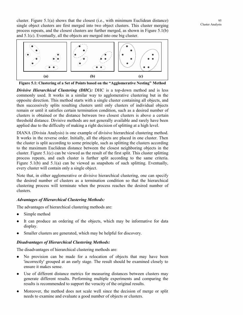
95

Cluster Analysis cluster. Figure 5.1(a) shows that the closest (i.e., with minimum Euclidean distance)

single object clusters are first merged into two object clusters. This cluster merging

process repeats, and the closest clusters are further merged, as shown in Figure 5.1(b)

and 5.1(c). Eventually, all the objects are merged into one big cluster.

(a) (b) (c)

Figure 5.1: Clustering of a Set of Points based on the “Agglomerative Nesting” Method

Divisive Hierarchical Clustering (DHC): DHC is a top-down method and is less

commonly used. It works in a similar way to agglomerative clustering but in the

opposite direction. This method starts with a single cluster containing all objects, and

then successively splits resulting clusters until only clusters of individual objects

remain or until it satisfies certain termination condition, such as a desired number of

clusters is obtained or the distance between two closest clusters is above a certain

threshold distance. Divisive methods are not generally available and rarely have been

applied due to the difficulty of making a right decision of splitting at a high level.

DIANA (Divisia Analysis) is one example of divisive hierarchical clustering method.

It works in the reverse order. Initially, all the objects are placed in one cluster. Then

the cluster is split according to some principle, such as splitting the clusters according

to the maximum Euclidean distance between the closest neighboring objects in the

cluster. Figure 5.1(c) can be viewed as the result of the first split. This cluster splitting

process repeats, and each cluster is further split according to the same criteria.

Figure 5.1(b) and 5.1(a) can be viewed as snapshots of such splitting. Eventually,

every cluster will contain only a single object.

Note that, in either agglomerative or divisive hierarchical clustering, one can specify

the desired number of clusters as a termination condition so that the hierarchical

clustering process will terminate when the process reaches the desired number of

clusters.

Advantages of Hierarchical Clustering Methods:

The advantages of hierarchical clustering methods are:

Simple method

It can produce an ordering of the objects, which may be informative for data

display.

Smaller clusters are generated, which may be helpful for discovery.

Disadvantages of Hierarchical Clustering Methods:

The disadvantages of hierarchical clustering methods are:

No provision can be made for a relocation of objects that may have been

'incorrectly' grouped at an early stage. The result should be examined closely to

ensure it makes sense.

Use of different distance metrics for measuring distances between clusters may

generate different results. Performing multiple experiments and comparing the

results is recommended to support the veracity of the original results.

Moreover, the method does not scale well since the decision of merge or split

needs to examine and evaluate a good number of objects or clusters.

96


The clustering quality of hierarchical method can be improved by integrating

hierarchical clustering with other clustering techniques for multiple phase clustering.

A few such methods are as follows:

BIRCH: It first partitions objects hierarchically using tree structures and then

applies other clustering algorithms to form refined clusters.

CURE: It represents each cluster by a certain fixed number of representative

points and then shrinks them toward the center of the cluster by a specified

fraction.

CHAMELEON: It explores dynamic modeling in hierarchical clustering.

BIRCH: Balanced Iterative Reducing and Clustering Using Hierarchies:

BIRCH was developed by Zhang, Ramakrishnan and Livny in 1996. It introduces two

concepts, clustering feature and CF tree (Clustering Feature tree). CF tree is used to as

a summarize cluster representation to achieve good speed and clustering scalability in

large databases. BIRCH is also good for incremental and dynamical clustering of

incoming data points.

A clustering feature (CF) is a triplet summarizing information about subclusters of

points. If there are N d-dimensional points Xi in a subcluster, CF is defined as:

CF = (n, LS, ss), where

LS =1

i

i n

X

å is the linear sum and ss

= 2

1

i

i n

X

å the square sum of the points.

Clustering feature is essentially summary statistics for the cluster: the zero-th, first,

and second moments of the subcluster from statistical point of view. It registers

crucial measurements for computing clusters and utilizes storage efficiently since it

summarizes the information about the subclusters of points instead of storing all

points.

CURE: Clustering Using Representatives:

Most clustering algorithms either favors clusters with spherical shape and similar

sizes, or are fragile in the presence of outliers. But the CURE (Clustering Using

Representatives) method integrates hierarchical and partitioning algorithms and

overcomes the problem of favoring clusters with spherical shape and similar sizes.

CURE employs a novel hierarchical clustering algorithm that adopts a middle ground

between the centroid-based and the all-point extremes. CURE measures the similarity

of two clusters based on the similarity of the closest pair of the representative points

belonging to different clusters, without considering the internal closeness (density or

homogeneity) of the two clusters involved. In CURE, a constant number c of well-

scattered points in a cluster are first chosen. The scattered points capture the shape and

extent of the cluster. The chosen scattered points are next shrunk towards the centroid

of the cluster by a fraction α . These scattered points after shrinking are used as

representatives of the cluster. The clusters with the closest pair of representative

points are the clusters that are merged at each step of CURE’s hierarchical clustering

algorithm.

The scattered points approach employed by CURE alleviates the shortcomings of both

the all-points as well as the centroid-based approaches. CURE is less sensitive to

outliers since shrinking the scattered points toward the mean dampens the adverse

effects due to outliers. Outliers are typically further away from the mean and are

thus shifted a larger distance due to the shrinking. Multiple scattered points also

enable CURE to discover non-spherical clusters like the elongated clusters. For the

97

Cluster Analysis centroid-based algorithm, the space that constitutes the vicinity of the single centroid

for a cluster is spherical. With multiple scattered points as representatives of a cluster,

the space that form the vicinity of the cluster can be non-spherical.

The kinds of cluster identify by CURE can be tuned by varying α from 0 to 1. If =

0 then CURE reduces to the centroid based algorithm. If = 1 then CURE becomes

similar to the all-points approach.

CURE produces high quality clusters in the existence of outliers, complex shapes of

clusters with different size. It scales well for large databases without sacrificing

clustering quality. CURE needs a few user-specified parameters, such as the size of

the random sample, the number of desired clusters, and the shrinking fraction a. One

question is the sensitivity of these parameters to the results of clustering. A sensitivity

analysis has been provided on the effect of changing parameters. It shows although

some parameters can be varied without impacting the quality of clustering, the

parameter setting in general does have a significant influence on the results.

CHAMELEON: A Hierarchical Clustering Algorithm Using Dynamic Modeling:

CHAMELEON (Clustering Using Dynamic Model) is a hierarchical clustering

algorithms which, measures the similarity of two clusters based on a dynamic model.

In the clustering process, two clusters are merged only if the inter-connectivity and

closeness (proximity) between two clusters are high relative to the internal inter-

connectivity of the clusters and closeness of items within clusters. The merging

process used by CHAMELEON using the dynamic model and facilitates discovery of

natural homogenous clusters.

CHAMELEON operates on a sparse graph in which nodes represents data items, and

weighted edges represent similarities among the data items. This sparse graph

representation of the data set allows CHAMELEON to scale large data sets and to

operate successfully on the data sets that are available only in similarity space. It finds

the clusters in the data set by using a two-phase algorithm. During the first phases, it

uses a graph-partitioning algorithm to cluster the data items into a large number of

relatively small sub-clusters.

It initially starts with all the points belonging to the same cluster. It then repeatedly

selects the largest sub-cluster among the current set of sub-clusters. This process

terminates when the larger sub-cluster contains less than a specified number of

vertices that is named minsize. The minsize parameter essentially controls the

granularity of the initial clustering solution. Minsize should be set to a value that is

smaller than the size of most of the sub-clusters expected to find in the dataset.

Minsize is used to be in the 1% and 5% range.

During the second phase, it uses an agglomerative hierarchical clustering algorithm to

find the genuine clusters by repeatedly combining together these sub-clusters.

CHAMELEON agglomerative hierarchical clustering algorithm determines the pair of

most similar sub-clusters by taking into accounts both the inter-connectivity as well as

the closeness of the clusters. The relative inter-connectivity between a pair of clusters

Ci and Cj is defined as the absolute inter-connectivity between Ci and Cj normalized

with respect to the internal inter-connectivity. The absolute interconnectivity between

a pair of clusters Ci and Cj is defined to be the sum of the weight of the edges that

connect vertices in Ci to vertices in Cj. The relative closeness between pair of clusters

Ci and Cj is defined as the absolute closeness between Ci and Cj normalized with

respect to the internal closeness of the two clusters Ci and Cj.

Chameleon measures the closeness of two clusters by computing the average

similarity between the points in Ci that are connected to points in Cj.

98



Fill in the blanks:

1. Hierarchical algorithms create a hierarchical decomposition of the

objects. They are either ………………………. or………………………. .

2. The main focus of ………………………. clustering algorithms is spatial

data, i.e., data that model the geometric structure of objects in space, their

relationships, properties and operations

3. ………………………. clustering algorithms are specifically developed

for data where Euclidean, or other numerical-oriented, distance measures

cannot be applied.

4. ………………………. variables are continuous measurements of a

roughly linear scale.

5. ……………… and CLARANS are based on the clustering criterion of

PAM.

5.9 PARTITIONAL ALGORITHMS

Given a database of n objects, and k, the number of clusters to form, a partitioning

algorithm organizes the objects into k partitions (k < n), where each partition

represents a cluster. The clusters are formed to optimize an objective-partitioning

criterion, often called a similarity function, such as distance, so that the objects within

a cluster are "similar", whereas the objects of different clusters are "dissimilar" in

terms of the database attributes.

Classical Partitioning Methods: k-means and k-medoids:

The most well-known and commonly used partitioning methods are k-means proposed

by (MacQueen 1967), and k-medoids proposed by (Kaufman and Rousseeuw 1987),

and their variations.

Centroid-based Technique: The k-means Method:

The goal in k-means is to produce k clusters from a set of n objects, so that the

squared-error objective function:

2

1

| – |i

k

p C i

i

E p m

å

In the above expression, Ci are the clusters, p is a point in a cluster Ci and the mean of

mi cluster Ci.

The mean of a cluster is given by a vector, which contains, for each attribute, the

mean values of the data objects in this cluster. Input parameter is the number of

clusters, k, and as an output the algorithm returns the centers or means, of every

cluster Ci most of the times excluding the cluster identities of individual points. The

distance measure usually employed is the Euclidean distance. Both for the

optimization criterion and the proximity index, there are no restrictions, and they can

be specified according to the application or the user’s preference. The k-mean

procedure is summarized in Figure 5.2 and the algorithm is as follows:

Select k _ objects as initial centers;

Assign each data object to the closest center;

Recalculate the centers of each cluster;

Repeat steps 2 and 3 until centers do not change;

99

Cluster Analysis The algorithm is relatively scalable, since its complexity is, i, O(1mn)

1, i, O(1kn)

1

where I denotes the number of iterations, and usually k << n.

(a)

(b)

(c)

Figure 5.2 (a), (b) and (c): Clustering a Set of Points based on the k-means Method

The algorithm attempts to determine k partitions that minimize the squared-error

function. It works well when the clusters are compact clouds that are rather well

separated from one another.

Example for k-mean method: Suppose there is a set of objects located in a rectangle

as shown in Figure 5.2, let k = 3. Now according to Algorithm k-mean, we arbitrarily

choose 3 objects (marked by "+") as the initial three cluster centers. Then each object

is distributed to the chosen cluster domains based on which cluster center is the

nearest. Such a distribution forms a silhouette encircled by dotted curve, as shown in

Figure 5.2(a).

This kind of grouping will update the cluster centers. That is, the mean value of each

cluster is recalculated based on the objects in the cluster. Relative to these new

centers, objects are re-distributed to the chosen cluster domains based on which

100


cluster center is the nearest. Such a re-distribution forms a new silhouette encircled by

dashed curve, as shown in Figure 5.2(b).

This process repeats, which leads to Figure 5.2(c). Eventually, no re-distribution of

the objects in any cluster happens and the process terminates. The final clusters are the

result of the clustering process.

There are quite a few variants of the k-means method, which differ in the selection of

initial k-means, the calculation of dissimilarity, and the strategies to calculate cluster

means. An interesting strategy, which often yields good results, is to first apply a

hierarchical agglomeration algorithm to determine the number of clusters and to find

an initial classification, and then use iterative relocation to improve the classification.

k-medoid algorithm: It is used for partitioning based on the central objects.

Input: The number of clusters k, and a database containing n objects.

Output: A set of k clusters which minimizes the sum of the dissimilarities of all the

objects to their nearest medoid.

The k-medoids algorithm is implemented as follows:

Arbitrarily choose k objects as the initial medoids

Repeat

Assign each object to the cluster corresponding to the nearest medoid;

Calculate the objective function, which is the sum of dissimilarities of all the

objects to their nearest medoid

Swap the medoid x by an object y if such a swap reduces the objective function

until no change.

The k-means algorithm is sensitive to outliers since an object with some extremely

large value may substantially distort the distribution of data. Instead of taking the

mean value of the objects in a cluster as a reference point, one may take a

representative object in a cluster, called a medoid, which is the most centrally located

point in a cluster. Thus the partitioning method can still be performed based on the

principle of minimizing the sum of the dissimilarities between each object and with its

corresponding reference point, which forms the basis of the k-medoids method.

Example for k-medoid method: Suppose there is a set of objects located in a rectangle

as shown in Figure. Let k = 3. Now according to Algorithm k-medoid, we arbitrarily

choose 3 objects (marked by "+") as the initial three cluster centers. Then each object

is distributed to the chosen cluster domains based on which cluster center is the

nearest. Such a distribution forms a silhouette encircled by dotted curve, as shown in

Figure 5.3(a).

This kind of grouping will update the cluster centers. That is, the medoid of each

cluster is recalculated based on the objects in the cluster. Regarding to these new

centers, objects are re-distributed to the chosen cluster domains based on which

cluster center is the nearest. Such a re-distribution forms a new silhouette encircled by

dashed curve, as shown in Figure 5.3(b).

This process repeats, which leads to Figure 5.3(c). Eventually, no re-distribution of

the objects in any cluster happens and the process terminates. The final clusters are the

result of the clustering process.

101

Cluster Analysis

(a)

(b)

(c)

Figure 5.3: Clustering a Set of Points based on the k-means Method

The k-medoids method is more robust than k-means in the presence of noise and

outliers because a medoid is less influenced by outliers or other extreme values than

mean. However, its processing is more costly than the k-means method. Moreover, it

also needs user to specify k, the number of clusters.

PAM (partition around medoids)

PAM is an extension to k-means, intended to handle outliers efficiently. Instead of

cluster centers, it chooses to represent each cluster by its medoid. A medoid is the

most centrally located object inside a cluster. As a consequence, medoids are less

influenced by extreme values; the mean of a number of objects would have to

“follow” these values while a medoid would not. The algorithm chooses _ medoids

initially and tries to place other objects in clusters whose medoid is closer to them,

while it swaps medoids with non-medoids as long as the quality of the result is

improved. Quality is also measured using the squared-error between the objects in a

cluster and its medoid. The computational complexity of PAM is, O(Ik(n–k)2), with l

being the number of iterations, making it very costly for large n and k values. Where, I

is the number of iterations.

102


Partitioning Methods in Large Databases: From k-medoids to CLARANS

A typical k-medoids partition algorithm like PAM works effectively for small data

sets, but it does not scale well for large data sets. More over, PAM is very costly for

large n and k values. To deal with larger data sets, a sampling-based method, called

CLARA (clustering large applications) was developed by (Kaufman and Rousseeuw

1990).

In case of CLARA, instead of taking the whole set of data into consideration, only a

small portion of the real data is chosen as a representative of the data, and medoids are

chosen from this sample using PAM. If the sample is selected in a fairly random

manner, it correctly represents the whole data set, and the representative objects

(medoids) chosen will therefore be similar to those chosen from the whole data set.

CLARA draws multiple samples of the data set, applies PAM on each sample, and

gives the best clustering as the output. As expected, CLARA can deal with larger data

sets than PAM. The complexity of each iteration now becomes O(kS2 + k(n — k)),

where S is the size of the sample, k is the number of clusters, and n is the total number

of points. It has been shown that CLARA works well with 5 samples of 40 + k size.

Note that there is a quality issue when using sampling techniques in clustering: the

result may not represent the initial data set, but rather a locally optimal solution. In

CLARA for example, if "true" medoids of the initial data are not contained in the

sample, then the result is guaranteed not to be the best.

To improve the quality and scalability of CLARA, another clustering algorithm called

CLARANS (Clustering Large Applications based upon Randomized Search) was

proposed by (Ng and Han 1994). It is also a k-medoids type algorithm and combines

the sampling technique with PAM. However, unlike CLARA, CLARANS does not

confine itself to any sample at any given time. While CLARA has a fixed sample at

every stage of the search, CLARANS draws a sample with some randomness in each

step of the search.

The clustering process can be presented as searching a graph where every node is a

potential solution, i.e., a set of k medoids. Two nodes are neighboring if they differ by

one medoid. The CLARANS approach works as follows:

Randomly choose k medoids;

Randomly consider one of the medoids to be swapped with a non-medoid;

If the cost of the new configuration is lower, repeat step 2 with new solution;

If the cost is higher, repeat step 2 with different non-medoid object, unless a limit

has been reached (the maximum value between 250 and k(n — k;

Compare the solutions so far, and keep the best;

Return to step 1, unless a limit has been reached (set to the value of 2).

CLARANS compares an object with every other, in the worst case and for every of

the k medoids. Thus, its computational complexity is, O(kn2), which does not make it

suitable for large data sets.

Figure 5.4: Three Applications of the k-means Algorithm

(a) Well separated Clusters (b) Clusters of different sizes (c) Arbitrary-Shaped clusters

103

Cluster Analysis Figure 5.4 presents the application of k-means on three kinds of data sets. The

algorithm performs well on appropriately distributed (separated) and spherical-shaped

groups of data (Figure 5.4 (a)). In case the two groups are close to each other, some of

the objects on one might end up in different clusters, especially if one of the initial

cluster representatives is close to the cluster boundaries (Figure 5.4 (b)). Finally, k-

means does not perform well on non-convex-shaped clusters (Figure 5.4 (c)) due to

the usage of Euclidean distance. As already mentioned, PAM appears to handle

outliers better, since medoids are less influenced by extreme values than means,

something that k-means fails to perform in an acceptable way.

CLARA and CLARANS are based on the clustering criterion of PAM, i.e., distance

from the medoid, working on samples of the data sets they are applied on, and making

them more scalable. However, their efficiency and effectiveness highly depend on the

sample size and its bias. A bias is present in a sample when the data objects in it have

not been drawn with equal probabilities.

Finally, their application is restricted to numerical data of lower dimensionality, with

inherent well separated clusters of high density.


What do you understand by the partition around medoids?

………………………………………….………………………………………

………………………………………….………………………………………

5.10 LET US SUM UP

A cluster is a collection of data objects that are similar to one another within the same

cluster and are dissimilar to the objects in other clusters. The process of grouping a set

of physical or abstract objects into classes of similar objects is called clustering.

Cluster analysis has wide applications including market or customer segmentation,

pattern recognition, biological studies, spatial data analysis, Web document

classification, and many others. Cluster analysis can be used as a stand-alone data

mining tool to gain insight into the data distribution, or serve as a preprocessing step

for other data mining algorithms operating on the detected clusters. The quality of

clustering can be assessed based on a measure of dissimilarity of objects, which can

be computed for various types of data, including interval-scaled, variables, binary

variables, nominal, ordinal, and ratio-scaled variables, or combinations of these

variable types. Clustering is a dynamic field of research in data mining, with a large

number of clustering algorithms developed.

These algorithms can be categorized into partitioning methods, hierarchical methods,

density-based methods, grid-based methods, and model-based methods. A partitioning

method first creates an initial k partition, where k is the number of partitions to

construct, then it uses an iterative relocation technique which attempts to improve the

partitioning by moving objects from one group to another. Typical partition methods

include k-means, k-medoids, CLARANS, and their improvements. A hierarchical

method creates a hierarchical decomposition of the given set of data objects. The

method can be classified as being either agglomerative (bottom-up) or divisive (top-

down), based on how the hierarchical decomposition is formed. To compensate the

rigidity of merge or split, hierarchical agglomeration often integrates other clustering

techniques, such as iterative relocation. Typical such methods include BIRCH, CURE,

and Chameleon.

A density-based method cluster objects based on the notion of density. It either grows

clusters according to density of neighborhood objects (such as in DBSCAN) or

according to some density function (such as in DENCLUE). Typical density-based

method include DBSCAN, OPTICS, and DENCLUE.

104


A grid-based method first quantizes the object space into a finite number of cells

which form a grid structure, and then performs clustering on the grid structure. STING

is a typical example of a grid-based method based on statistical information stored in

grid cells. CLIQUE and Wave-Cluster are two clustering algorithms which are both

grid-based and density-based.

A model-based method hypothesizes a model for each of the clusters and finds the

best fit of the data to that model. Typical model-based methods include statistical

approach, such as AutoClass, COBWEB and CLASSIT, and neural network approach,

such as SOM. One person’s noise could be another person’s signal. Outlier detection

and analysis is very useful for fraud detection, customized marketing, medical

analysis, and many other tasks. Computer-based outlier analysis methods typically

follow either a statistical approach, a distance-based approach, or a deviation-based

approach PAM (partition around medoids) is an extension to k-means, intended to

handle outliers efficiently.

A typical k-medoids partition algorithm like PAM works effectively for small data

sets, but it does not scale well for large data sets. More over, PAM is very costly for

large n and k values. To deal with larger data sets, a sampling-based method, called

CLARA (clustering large applications) was developed by (Kaufman and Rousseeuw

1990). A hierarchical clustering method works by grouping data objects into a tree of

clusters. Hierarchical clustering algorithms are either top-down or bottom-up. In

general, there are two types of hierarchical clustering methods. AHC is a bottom-up

clustering method where clusters have sub-clusters, which in turn have sub-clusters,

etc. It starts by placing each object in its own cluster and then merges these atomic

clusters into larger and larger clusters until all the objects are in a single cluster or

until it satisfies certain termination condition. Most hierarchical clustering methods

belong to this category. They differ only in their definition of between-cluster

similarity. DHC is a top-down method and is less commonly used. It works in a

similar way to agglomerative clustering but in the opposite direction.

DIANA (Divisia Analysis) is one example of divisive hierarchical clustering method.

The clustering quality of hierarchical method can be improved by integrating

hierarchical clustering with other clustering techniques for multiple phase clustering.

A few such methods are BIRCH, CURE and CHAMELEON.


Discuss hierarchical method of cluster analysis.

5.12 KEYWORDS

Clustering: The technique of grouping records together based on their locality and

connectivity within the n-dimensional space. This is an unsupervised learning

technique.

Collinearity: The property of two predictors showing significant correlation without a

causal relationship between them.

Nearest Neighbor: A data mining technique that performs prediction by finding the

prediction value of records (near neighbors) similar to the record to be predicted.

Partitioning Methods: Given a database of n objects or data tuples, a partitioning

method constructs k partitions of the data, where each partition represents a cluster,

and k < n.

The k-means Algorithm, where each cluster is represented by the mean value of the

objects in the cluster.

The k-medoids Algorithm, where each cluster is represented by one of the objects

located near the center of the cluster.

105

Cluster Analysis Hierarchical Method creates a hierarchical decomposition of the given set of data

objects.

Grid-based Methods quantize the object space into a finite number of cells which

form a grid structure.

Partitioning Methods: A partitioning clustering algorithm constructs partitions of the

data, where each cluster optimizes a clustering criterion, such as the minimization of

the sum of squared distance from the mean within each cluster.

Hierarchical Methods: Hierarchical algorithms create a hierarchical decomposition of

the objects.

Density-based Clustering Algorithms: These algorithms group objects according to

specific density objective functions.

Grid-based Clustering: The main focus of these algorithms is spatial data, i.e., data

that model the geometric structure of objects in space, their relationships, properties

and operations.

Model-based Clustering: These algorithms find good approximations of model

parameters that best fit the data.

Categorical Data Clustering: These algorithms are specifically developed for data

where Euclidean, or other numerical-oriented, distance measures cannot be applied.

PAM (Partition Around Medoids): PAM is an extension to k-means, intended to

handle outliers efficiently. Instead of cluster centers, it chooses to represent each

cluster by its medoid.

CLARANS: A typical k-medoids partition algorithm like PAM works effectively for

small data sets, but it does not scale well for large data sets.

Agglomerative Hierarchical Clustering (AHC): AHC is a bottom-up clustering

method where clusters have sub-clusters, which in turn have sub-clusters, etc.

Divisive Hierarchical Clustering (DHC): DHC is a top-down method and is less

commonly used.

DIANA (Divisia Analysis): DIANA is one example of divisive hierarchical clustering

method.

BIRCH: It first partitions objects hierarchically using tree structures and then applies

other clustering algorithms to form refined clusters.

CURE: It represents each cluster by a certain fixed number of representative points

and then shrinks them toward the center of the cluster by a specified fraction.

CHAMELEON: It explores dynamic modeling in hierarchical clustering.

Clustering Feature (CF): It is a triplet summarizing information about subclusters of

points.


1. Explain the basic idea of clustering with suitable example.

2. What is clustering? How is it different from classification?

3. Briefly outline how to compute the dissimilarity between objects described by the

following types of variables:

(a) Asymmetric binary variables

(b) Nominal variables

(c) Ratio-scaled variables

(d) Numerical (interval-scaled) variables

106


4. Briefly describe the following approaches to clustering methods: partitioning

methods, hierarchical methods, density-based methods, grid-based methods, and

model-based methods. Give examples in each case.

5. Data cubes and multidimensional databases contain categorical, ordinal, and

numerical data in hierarchical or aggregate forms. Based on what you have

learned about the clustering methods, design a clustering method which finds

clusters in large data cubes effectively and efficiently.

6. What do you mean by Outlier Analysis? Explain with the help of suitable

example.

7. Write short notes on the following:

(a) Categorization of major clustering methods

(b) Density-based Clustering

(c) Grid-based Clustering

(d) Model-based Clustering

(e) Categorical Data Clustering

(f) Centroid-based technique: The k-means method

(g) k-medoid algorithm

(h) PAM (Partition Around Medoids)

(i) CLARA

(j) Agglomerative Hierarchical Clustering (AHC)

(k) Divisive Hierarchical Clustering (DHC)


CYP 1

Major clustering methods can be classified into the following categories:

(a) Partitioning Methods

(b) Hierarchical Methods

(c) Density-based Clustering

(d) Grid-based Methods

CYP 2

1. Agglomerative, Divisive

2. Grid based

3. Categorical data

4. Interval-scaled

5. CLARA

CYP 3

PAM is an extension to k-means, intended to handle outliers efficiently.

Instead of cluster centers, it chooses to represent each cluster by its medoid. A

medoid is the most centrally located object inside a cluster.





1993.

107

Cluster Analysis









108


LESSON

6 ASSOCIATION RULES

CONTENTS


6.1 Introduction

6.2 Large Item Set Basic Algorithms

6.3 Parallel & Distributed Algorithms

6.4 Discussion of Parallel Algorithms

6.5 Comparing Approaches

6.6 Incremental Rules

6.7 Advance Association Rule Techniques

6.8 Measuring the Quality of Association Rules

6.9 Let us Sum up


6.11 Keywords





The concept of association rule of data mining

Basic knowledge of parallel & distributed algorithms

Various types of association rules

6.1 INTRODUCTION

One of the reasons behind maintaining any database is to enable the user to find

interesting patterns and trends in the data. For example, in a supermarket, the user can

figure out which items are being sold most frequently. But this is not the only type of

‘trend’ which one can possibly think of. The goal of database mining is to automate

this process of finding interesting patterns and trends. Once this information is

available, we can perhaps get rid of the original database. The output of the data-

mining process should be a “summary” of the database. This goal is difficult to

achieve due to the vagueness associated with the term ‘interesting’. The solution is to

define various types of trends and to look for only those trends in the database. One

such type constitutes the association rule.

In the rest of the discussion, we shall assume the supermarket example, where each

record or tuple consists of the items of a single purchase. However the concepts are

applicable in a large number of situations.

109

Association Rules In the present context, an association rule tells us about the association between two or

more items. For example, in 80% of the cases when people buy bread, they also buy

milk. This tells us of the association between bread and milk. We represent it as:

bread milk | 80%

This should be read as - “Bread means or implies milk, 80% of the time.” Here 80% is

the “confidence factor” of the rule.

6.2 LARGE ITEM SET BASIC ALGORITHMS

We assume data is too large to fit in main memory. Either it is stored in a RDB, say as

a relation Baskets (BID; item) or as a flat file of records of the form (BID; item1;

item2; : : : ; itemn). When evaluating the running time of algorithms we:

Count the number of passes through the data. Since the principal is often the time

it takes to read data from disk, the number of times we need to read each datum I

soften the best measure of running of the algorithm.

There is a key principle called monotonicity or the a-priori trick that helps us find

frequent itemsets:

Is a set of items S is frequent (i.e. appears in at least fraction s of the baskets),

then every subset of S is also frequent.

To find frequent itemsets, we can:

Proceed levelwise, finding first the frequent items (sets of size 1), then the

frequent pairs the frequent triples, etc. we concentrate on finding frequent pairs

because:

Often, pairs are enough

In many data sets, the hardest part is finding the pairs: proceeding to higher

levels takes less time than finding frequent pairs.

Find all maximal frequent itemsets (e.g., sets S such that no proper subset fo S in

frequent) in one pass or a passes.

6.3 PARALLEL & DISTRIBUTED ALGORITHMS

Parallel and distributed algorithms for mining association rules can be classified in

terms of three main components:

Distributed versus shared memory system.

Data versus task parallelism

Static versus dynamic load balancing

In a distributed (shared-nothing) memory architecture each processor has a private

memory and a message passing mechanism needs to be employed for exchanging data

between processors. In a shared memory architecture, in contrast, all processors can

access a common memory. In a distributed memory system, communication between

the processors is crucial to accomplish tasks. Parallel algorithms geared toward these

systems are often concerned with portioning the candidate sets to processor memories,

reducing communication, and pruning candidate sets. In a shared memory system,

however, communication cost is no longer an issue, since processors communicate

through shared variables. Instead, performance is determined by I/O and computation

costs. Unfortunately, I/O can become a bottleneck due to the access of different

processes via the same I/O channel. Also I/O contention may result due to a

synchronized access of processors. On the other hand, with its large aggregated

memory, a shared memory processor is good for mining association rules that need

large storage for storing intermediate values.

110


Data and task parallelism split according to the distribution of candidate sets across

the processors. While each processor counts the same set of candidates in a data

parallel algorithm, each processor in a task parallel algorithm counts a different set of

distributed candidates. With data parallelism the database is portioned among the

processors and with task parallelism, each processor has or needs access to the entire

database.

Parallel algorithms can further be classified as having a static or dynamic load

balancing. Static load balancing refers to the initial and final portioning of the

database among processors according to some heuristic cost function. In contrast,

dynamic load balancing refers to the environment where data is continuously moved

from heavily loaded processors to less busy ones. Current association rule mining

algorithms all employ static load balancing, since they partition the database among

processors and assume a homogeneous environment. The taxonomy of different

parallel and distributed algorithms according to these three components is given in

Figure 6.1.

Figure 6.1: Taxonomy of Parallel Association Rule Mining Algorithms

Data Parallel Algorithms on Distributed Memory Systems:

The algorithms that adopt the data parallelism paradigm on a distributed memory

architecture include Count Distribution (CD) proposed by Parallel Data Mining

(PDM), and Distributed Mining of Association Rules (DMA).

Data Parallel Algorithms on Shared Memory Systems:

Shared memory multiprocessors are useful for association rule mining, since they

have large aggregate memory. The algorithms developed for machines with this type

of architecture are not concerned with communication cost due to the communication

of processors via shared variables. Hence, the main objectives of algorithms targeting

this architecture are to reduce computation and I/O contention caused by

synchronization. One of the first data parallel algorithms for shared memory

multiprocessors is the Common Candidate Partitioned Database (CCPD).

Task Parallel Algorithms on Shared Memory Systems:

Task parallel algorithms designed for shared memory systems include Partitioned

Candidate Common Database (PCCD), and Asynchronous Parallel Mining (APM).

111

Association Rules 6.4 DISCUSSION OF PARALLEL ALGORITHMS

The main challenges parallel and distributed algorithms face today include

communication overhead minimization, synchronization, workload balancing, data

decomposition, efficient memory usage and disk I/O minimization. Various

algorithms have been proposed that explore trade-offs between these issues.

6.5 COMAPRING APPROACHES

There are three main approaches to data mining.

"I suspect that...":

Sometimes called verification or exploratory data mining.

An analyst has a hypothesis, and uses data to verify it, or partially verify it.

This leads to a revised hypothesis, which begins the process again.

Response time is important so that trains of thought can be followed. The

approach is mostly based on OLAP technology.

"I know who, now tell me why, OR now predict who else...":

This is based on existing practices which are reasonably well understood. Such

techniques are called supervised, because the algorithms train on customers who

are known to have some property X.

The transparent approach: these are my customers with property X, now tell me

what else they have in common.

The opaque approach: give me a black box that identifies (new) customers with

property X.

Examples: churn reduction (contract renewal), automated judgement (mortgage

approval, medical billing), targeting (bulk mailing, retail marketing).

Transparent approaches may be more useful, but require more sophistication to

exploit.

"Tell me something interesting...":

Here the algorithm is to find hypotheses that are likely given the available data,

and also interesting, i.e. unlikely to have occurred by chance. Such techniques are

called unsupervised.

Typical outcomes are of the form "there is a cluster of customers with the

following characteristics".

Examples: market segmentation, unsuspected correlations.

This approach seems to have the greatest potential since it provides information

that is not accessible in any other way.

Data mining algorithms can be regarded abstractly as either:

Mappings from data to concepts (i.e. predicates) in transparent approaches;

Mappings from data to parameters of a model in opaque approaches.

There are also important pre- and post processing issues:

Data preparation, e.g what to do about missing values;

Winnowing, e.g. some techniques produce more concepts than the input.

These issues are the same for both sequential and parallel data mining, so we

won't address them explicitly.

112


6.6 INCREMENTAL RULES

In many data mining tasks the underlying data cannot be assumed to be static,

although most data mining algorithms, such as Apriori, are designed for static data set

and updates to the data are handled by running the algorithm again. This is not

acceptable for large data sets, or when the runtime is slow. Algorithms are needed that

can handle incremental updates to the data is a graceful manner.

Fast Update (FUP) is one approach to association rules that handles incremental

updates to the data. The method tries to determine the promising itemsets in the

incremental update to reduce the size of the candidate set to be searched in the original

large database.

Given the initial large database DB with known itemsets L, an incremental update db

is to be added to it. Some previously large k-itemsets may become small in DB + db,

whereas some previously small ones may become large. An itemset will be large if it

is large in both DB and db, and it will be small if it is small in both. The itemsets that

are large in DB, but small in db just need to have the counts updated using the counts

from db. Moreover, the itemsets that are large only in db need to be checked for

sufficient support, requiring a scan of the large DB to get the count. Using these

updated counts, the support and confidence for the itemsets can then be computed.

6.7 ADVANCE ASSOCIATION RULE TECHNIQUES

Association rules use a concept hierarchy, i.e., building rules at different levels of the

hierarchy. One possible motivation would be when there is insufficient support for a

rule involving the actual items, there might be sufficient support for the ancestors of

the item.

In Figure 6.2, a simple hierarchy is shown, and a set of transactions based on the items

is presented in Table 6.1. In Table 6.2, each transaction has been extended to include

the hierarchy. Standard algorithms such as Apriori can be applied to the extended

transactions to generate the association rules. Note that support for an ancestor is not

simply the sum of the support for the children because several of the children could be

presented in a single transaction.

Figure 6.2: Hierarchy for Cloths and Footwear

Table 6.1: The Original Transactions

Transaction Items Bought

100 Shirt

200 Jacket, Hiking Boots

300 Ski Pants, Hiking Boots

400 Shoes

500 Shoes

600 Jacket

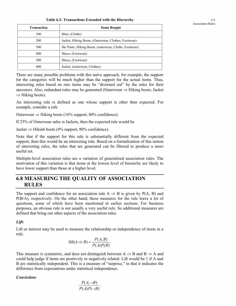
113

Association Rules

Table 6.2: Transactions Extended with the Hierarchy

Transaction Items Bought

100 Shirt, (Cloths)

200 Jacket, Hiking Boots, (Outerwear, Clothes, Footwear)

300 Ski Pants, Hiking Boots, (outerwear, Cloths, Footwear)

400 Shoes, (Footwear)

500 Shoes, (Footwear)

600 Jacket, (outerwear, Clothes)

There are many possible problems with this naïve approach, for example, the support

for the categories will be much higher than the support for the actual items. Thus,

interesting rules based on rare items may be “drowned out” by the rules for their

ancestors. Also, redundant rules may be generated (Outerwear Hiking boots; Jacket

Hiking boots).

An interesting rule is defined as one whose support is other than expected. For

example, consider a rule

Outerwear Hiking boots (16% support, 80% confidence).

If 25% of Outerwear sales is Jackets, then the expected rule would be

Jacket Hikinh boots (4% support, 80% confidence).

Note that if the support for this rule is substantially different from the expected

support, then this would be an interesting rule. Based on a formalization of this notion

of interesting rules, the rules that are generated can be filtered to produce a more

useful set.

Multiple-level association rules are a variation of generalized association rules. The

motivation of this variation is that items at the lowest level of hierarchy are likely to

have lower support than those at a higher level.

6.8 MEASURING THE QUALITY OF ASSOCIATION

RULES

The support and confidence for an association rule A B is given by P(A, B) and

P(B/A), respectively. On the other hand, these measures for the rule leave a lot of

questions, some of which have been mentioned in earlier sections. For business

purposes, an obvious rule is not usually a very useful rule. So additional measures are

defined that bring out other aspects of the association rules.

Lift:

Lift or interest may be used to measure the relationship or independence of items in a

rule.

( , )lift( ) .

( ) ( )

P A BA B

P A P B

This measure is symmetric, and does not distinguish between A B and B A and

could help judge if items are positively or negatively related. Lift would be 1 if A and

B are statistically independent. This is a measure of “surprise,” in that it indicates the

difference from expectations under statistical independence.

Conviction:

( , ).

( ) ( )

P A B

P A P B

114


From symbolic logic, it is known that A → B ≡ ~(A ^ ~ B). So,

Would measure the negation of A → B. To account for negation, the fraction is

inverted to measure conviction.

( , )conviction( ) .

( ) ( )

P A BA B

P A P B

When A and B are not related, all the events are independent, and conviction will have

the value of 1. Rule that are always true approach ∞. Therefore, conviction measures

how strongly a rule holds.

Check Your Progress

Fill in the blanks:

1. ………………… is the discovery of association relationships or

correlations among a set of items.

2. Association rule mining finds interesting association or correlation

relationships among a ………………… set of data items.

3. A typical example of association rule mining is ………………… .

4. ………………… and ………………… are used to measure the quality of

a given rule, in terms of its usefulness (strength) and certainty.

5. An association rule is an implication of the form …………………, where

A I, B I and A B = .

6.9 LET US SUM UP

Discovery of association rules is an important task in data mining, since computing

large itemsets sequentially is costly in terms of I/O and CPU resources, there is a

practical need for scalable parallel algorithms especially when database are enormous

and distributed. Various parallel and distributed methods have been developed that

attempt to minimize communication, employ efficient computation, and

synchronization techniques, and make a better usage of memory on both distributed

and shared memory systems. Nevertheless there is still room for plenty of

improvement for solving issues including high dimensionality, large database sizes,

data location, data skew, and dynamic load balancing.


Discuss lift method of measuring the quality of association rules.

6.11 KEYWORDS

Association: Association is the discovery of association relationships or correlations

among a set of items. They are often expressed in the rule form showing attribute-

value conditions that occur frequently together in a given set of data. An association

rule in the form of X Y is interpreted as ‘database tuples that satisfy X are likely to

satisfy Y’.

Association rule mining: Association rule mining finds interesting association or

correlation relationships among a large set of data items.

Market basket analysis: A typical example of association rule mining is market

basket analysis. This process analyzes customer’s buying habits by finding

associations between the different items that customers place in their “shopping

baskets”.

115

Association Rules Support and confidence: These terms are used ed to measure the quality of a given

rule, in terms of its usefulness (strength) and certainty.


1. What is association? What do you understand by association analysis?

2. Why association rule mining is used in data mining?

3. What is market basket analysis? Give one example.

4. Define the terms “support” and “confidence”.

5. List out the various kinds of association rules and explain each with the help of

example.


1. Association

2. Large

3. Market basket analysis

4. Support, confidence

5. A B





1993.












Edition, 2004.


Publications, 2004.




Edition, 2000.

118


117

Data Warehouse

UNIT IV

118


119

Data Warehouse LESSON

7 DATA WAREHOUSE

CONTENTS


7.1 Introduction

7.2 Characteristics of Data Warehouse

7.3 Data Marts and Other Aspects of Data Mart

7.4 OLTP: Online Transaction Processing

7.4.1 OLTP System

7.4.2 OLTP and Data Warehousing

7.5 OLAP: Online Analytical Processing

7.5.1 Characteristics of OLAP

7.5.2 OLAP Data Modelling

7.6 Star Schema for Multidimensional View

7.7 Data Modelling – Multifact Star Schema or Snow Flake Schema

7.8 Categories of OLAP Tools

7.8.1 MOLAP

7.8.2 ROLAP

7.8.3 Managed Query Environment (MQE)

7.9 State of the Market

7.9.1 Cognos PowerPlay

7.9.2 IBI Focus Fusion

7.9.3 Pilot Software

7.9.4 Arbor Essbase Web

7.9.5 Information Advantage Web OLAP

7.9.6 Microstrategy DSS Web

7.9.7 Brio Technology

7.10 OLAP Tools and the Internet

7.11 Let us Sum up


7.13 Keywords





The concept of data warehouse

Characteristics of data warehousing

120


Basic knowledge of data marts

The concept of OLAP and OLTP

7.1 INTRODUCTION

Data mining potential can be enhanced if the appropriate data has been collected and

stored in a data warehouse. A data warehouse is a relational database management

system (RDBMS) designed specifically to meet the needs of transaction processing

systems. It can be loosely defined as any centralized data repository which can be

queried for business benefits but this will be more clearly defined later. Data

warehousing is a new powerful technique making it possible to extract archived

operational data and overcome inconsistencies between different legacy data formats.

As well as integrating data throughout an enterprise, regardless of location, format, or

communication requirements it is possible to incorporate additional or expert

information. It is,

The logical link between what the managers see in their decision support EIS

applications and the company’s operational activities.

– John McIntyre of SAS Institute Inc.

In other words the data warehouse provides data that is already transformed and

summarized, therefore making it an appropriate environment for more efficient DSS

and EIS applications.

7.2 CHARACTERISTICS OF DATA WAREHOUSE

According to Bill Inmon, author of Building the data Warehouse and the guru who is

widely considered to be the originator of the data warehousing concept, there are

generally four characteristics that describe a data warehouse:

Subject oriented: Data are organized according to subject instead of application

e.g. an insurance company using a data warehouse would organize their data by

customer, premium, and claim, instead of by different products (auto, life, etc.).

The data organized by subject contain only the information necessary for decision

support processing.

Integrated: When data resides in many separate applications in the operational

environment, encoding of data is often inconsistent. For instance, in one

application, gender might be coded as “m” and “f” in another by 0 and 1. When

data are moved from the operational environment into the data warehouse,

they assume a consistent coding convention e.g. gender data is transformed to “m”

and “f”.

Time variant: The data warehouse contains a place for storing data that are five to

ten years old, or older, to be used for comparisons, trends, and forecasting. These

data are not updated.

Non-volatile: Data are not updated or changed in any way once they enter the data

warehouse, but are only loaded and accessed.

7.3 DATA MARTS AND OTHER ASPECTS OF DATA MART

A data mart is a collection of subject areas organized for decision support based on the

needs of a given department. Finance has their data mart, marketing has theirs, sales

has theirs and so on. And the data mart for marketing only faintly resembles anyone

else’s data mart.

121

Data Warehouse Perhaps most importantly the individual departments OWN the hardware, software,

data and programs that constitute the data mart. The rights of ownership allows the

departments to bypass any means of control or discipline that might coordinate the

data found in the different departments.

Each department has its own interpretation of what a data mart should look like and

each department’s data mart is peculiar to and specific to its own needs. Typically, the

database design for a data mart is built around a star-join structure that is optimal for

the needs of the users found in the department. In order to shape the star join, the

requirements of the users for the department must be gathered. The data mart contains

only a modicum of historical information and is granular only to the point that it suits

the needs of the department. The data mart is typically housed in multidimensional

technology which is great for flexibility of analysis but is not optimal for large

amounts of data. Data found in data marts is highly indexed.

There are two kinds of data marts-dependent and independent. A dependent data mart

is one whose source is a data warehouse. An independent data mart is one whose

source is the legacy applications environment. All dependent data marts are fed by the

same source the data warehouse. Each independent data mart is fed uniquely and

separately by the legacy applications environment. Dependent data marts are

architecturally and structurally sound. Independent data marts are unstable and

architecturally unsound, at least for the long haul. The problem with independent data

marts is that their deficiencies do not make themselves manifest until the organization

has built multiple independent data marts.


1. What is a data warehouse?

…………………………………..………………………………………….

…………………………………..………………………………………….

2. Define Data mart.

…………………………………..………………………………………….

…………………………………..………………………………………….

7.4 OLTP: ONLINE TRANSACTION PROCESSING

Databases must often allow the real-time processing of SQL transactions to support e-

commerce and other time-critical applications. This type of processing is known as

online transaction processing (OLTP).

Queries used for OLTP and for DSS (decision support system) have different

performance requirements. OLTP queries are relatively less complex and the desired

response time is anywhere from split seconds to a few minutes. DSS queries, on the

other hand, are more complex and their response time can be from a few minutes to

many hours. Because of their difference in usage and the performance requirements,

OLTP and DSS used to be handled on different systems. Today, the increasing

complexity of business requirements and the pressure to lower the total cost of

ownership are requiring the data servers to move toward a mixed workload

environment where the OLTP system also performs the duties of decision support

system. These mixed workload environments are also called operational decision

support systems.

122


7.4.1 OLTP System

OLTP systems designed to maximise transaction capacity but they:

cannot be repositories of facts and historical data for business analysis

cannot quickly answer ad hoc queries

rapid retrieval is almost impossible

data is inconsistent and changing, duplicate entries exist, entries can be

missing

OLTP offers large amounts of raw data which is not easily understood

Typical OLTP query is a simple aggregation e.g.

what is the current account balance for this customer?

7.4.2 OLTP and Data Warehousing

Comparison between OLTP and Data Warehousing are:

Characteristics OLTP Data Warehousing

Purpose Run day-to-day operation Information retrieval and analysis

Structure RDBMS RDBMS

Data Model Normalized Multi-dimensional

Access SQL SQL Pluse data analysis extension

Type of Data Data that runs the business Data that analyses the business

Condition of Data Changing incomplete Historical, descriptive

7.5 OLAP: ONLINE ANALYTICAL PROCESSING

OLAP is a category of technology that enables users to gain insight into their data in a

fast, interactive, easy-to-use manner, rather than think of the data in terms of flat files

or spreadsheets, an OLAP application allows you to look at the data in terms of the

many dimensions. A flat file is a collection of text data stored line by line and always

read from start to finish. A dimensions is some way to locate the value of a

performance measure. This ability to organize the data in the way users think about it

is known as multidimensionality. This is what distinguishes OLAP capability from a

traditional system. For example, you could classify a sale by the purchase occurred

and the price of the product. Each one of these items could be thought of as a

dimension within the database. In this example, you have four dimensions:

Time

Product

Geography

Price

The key to the OLAP database is its dimensions. When you plug in the various

dimensions, the intersection of multiple dimensions produces a location called a cell.

That cell contains the intersecting values within all the dimensions. A cell is a single

data point that occurs at the intersection defined by selecting one value from each

dimension in a multidimensional array. In our example, we have time, product,

geography and price as dimensions. This means the dimensional members May 1996

(time), Maruti (product), and Mumbai (geography) specify a precise intersection along

all the dimensions that uniquely identify a single cell. In this example, the cell

contains the value of all Maruti sales in Mumbai for May 1996.

123

Data Warehouse Locating the value of sales Mumbai is easy. Think of it in terms of its position in the

database, as opposed to thinking about which columns you might have to join.

Each intersection of all the dimensions creates a cell; it is possible the cell is empty.

When the cell is empty, this is known as sparsity. In fact, it’s possible given a large

number cells, the greater the impact on performance. To get around this issue, the

vendors have implemented many ingenious techniques. This issue is one of the major

data sets. Knowing the position up front will get you to the answer much quicker. Yes,

you can make these types of relationships work in a traditional relational database, but

SQL is not a natural way of addressing these types of structures.

7.5.1 Characteristics of OLAP

The FASMI Test

We wanted to define the characteristics of an OLAP application in a specific way,

without dictating how it should be implemented.

Fast: Means that the system is targeted to deliver most responses to users within

about five seconds, with the simplest analysis taking no more than one second and

very few taking more than 20 seconds. Independent research in the Netherlands has

shown that end-users assume that a process has failed if results are not received with

30 seconds, and they are apt to hit ‘ALT+Ctrl+Delete’ unless the system wants them

that the report will take longer. Even if they have been wanted that it will take

significantly longer, users are likely to get distracted and t=lose their chain of thought,

so the quality of analysis suffers. This speed is not easy to achieve with large amounts

of data, particularly if on-the-fly and ad hoc calculations are required. Vendors resort

to a wide variety of techniques to achieve this goal, including specialized forms of

data storage, extensive pre-calculations and specific hardware expect this to be an area

of developing technology. In particular, the full pre-calculation approach fails with

very large, sparse applications as the database simply get too large (data base

explosion problem), whereas doing as the database simply is much too slow with large

database, even if exotic hardware is used. Even though minutes, users soon get bored

waiting and the project will be much less, successful than if it had delivered a near

instantaneous response, even at the cost of less detailed analysis.

Analysis: Means that the system can cope with any business logic and statistical

analysis that it relevant for the application and the user, the keep it easy enough for the

target user. Although some pre-programming may be needed, we do not think it

acceptable if all application definitions have to be done using a professional 4GL. It is

certainly necessary to allow the user to define new ad hoc calculations as part of the

analysis and to report on the data in any desired way, without having to program, so

we exclude products (like Oracle Discoverer) that do not allow the user to define new

ad hoc calculations as part of the analysis and to report on the data in any desired way,

without having to program, so we exclude products (like Oracle Discoverer) that do

not allow adequate end-user oriented calculation flexibility. We do not mind whether

this analysis is done in the vendor’s own tools or in a linked external product such as a

spreadsheet, simply that all the required analysis functionality be provided in an

intuitive manner for the target users. This could include specific features like time

series analysis, cost allocations, currency translation, goal seeking, ad hoc

multidimensional structural changes, non-procedural modeling, exception altering,

data mining and other application dependent features. These capabilities differ widely

between products, depending on their target markets.

Shared: Means that the system implements all the security requirements for

confidentiality (possibly down to cell level) and, multiple write access is needed,

concurrent update location at an appropriate level. Not all applications need users to

write data back, but for the growing number that do, the system should be able to

handle multiple updates in a timely, secure manner. This is a major area of weakness

124


in many OLAP products, which tend to assume that all OLAP applications will be

read-only, with simplistic security controls. Even products with multi-user read-write

often have crude security models; and example is Microsoft OLAP Services.

Multidimensional: Is our key requirement. If we have to pick a one-word definition

of OLAP this is it. The system must provide a multidimensional conceptual view of

the data, including full support for support for hierarchies and multiple hierarchies.

We are not setting up a specific minimum number of dimensions that must be handled

as it is too application dependent and most products seem to have enough for their

target markets. Again, we do not specify what underlying database technology should

be used providing that the user gets a truly multidimensional conceptual view.

Information: Is all of the data and derived information needed, whether it is and

however much is relevant for the application. We are measuring the capacity of

various products in terms of how much input data can handle, not how many

Gigabytes they take to store it. The capacities of the products differ greatly – the

largest OLAP products can hold at least a thousand times as much data as the

smallest. There are many considerations here, including data duplication, RAM

required, disk space utilization, performance, integration with data warehouses and the

like.

FASMI test is a reasonable and understandable definition of the goals OLAP is meant

to achieve. We encourage users and vendors to adopt this definition, which we hope

will avoid controversies of previous attempts.

The techniques used to achieve it include many flavors of client/server architecture,

time series analysis, object-orientation, optimized proprietary data storage,

multithreading and various patented ideas that vendors are so proud of. We have

views on these as well, but we would not want any such technologies to become part

of the definition of OLAP. Vendors who are covered in this report had every chance

to tell us about their technologies, but it is their ability to achieve OLAP goals for

their chosen application areas that impressed us most.

7.5.2 OLAP Data Modelling

In order to perform data modeling for OLAP, let us first examine some significant

characteristics of data in such a system. Review the following list highlighting

differences between OLAP and warehouse data:

An OLAP system stores and uses much less data compared with a data

warehouse.

Data in an OLAP system is summarized. The lowest level of detail as in the data

warehouse is very infrequent.

Every instance of the OLAP system is customized for the purpose that instance

serves. In other words, OLAP tends to be more departmentalized, whereas data in

the data warehouse serves corporate-wide needs.

Implementation Considerations: Before we specially focus on modeling for OLAP,

let us go over a few implementation issues. An overriding principle is that OLAP data

is generally customized. When you build an OLAP system with system interfaces

serving different user groups, this is an important point. For example, one instance or

specific set of summarizations would be meant to the preparation of OLAP data for a

specific group of users, say the marketing department.

125

Data Warehouse The following techniques apply to the preparation of OLAP data for a specific group

of users or a particular department such as marketing.

Define Subset: Select the subset of detailed data the marketing department is

interested in.

Summarize: Summarize and prepare aggregate data structures in the way the

marketing department needs for combining. For example, summarize products

along product categories as defined by marketing. Sometimes, marketing and

accounting departments may categorize products in different ways.

Denormalize: Combine relational tables in exactly the same way the marketing

department needs denormalized data.

Calculate and Derive: If some calculations and derivations of the metrics are

department-specific, use the ones for marketing.

OLAP Data Types and Levels: The OLAP data structure contains levels of

summarization and a few kinds of detailed data. You need to model these levels of

summarization and details.

The types and levels shown in Figure must be taken into consideration while

performing data modeling for OLAP systems. Pay attention to the different types of

data in an OLAP system. When you model the data structure for your OLAP system,

you need to provide fro these types of data.

Data Modeling for MOLAP: As a prerequisite to creation and storage of hypercubes

in proprietary MDDBs, data must be in the form of multidimensional representations.

You need to consider special requirements of the selected MDDBMS for data input

for creation.

7.6 STAR SCHEMA FOR MULTIDIMENSIOANL VIEW

The dominating conceptual data model for data warehouses is the multidimensional

view, based on two factors: a set of mostly numeric measures that define the objects

associated with the subject areas (e.g., sales-total, customer-id, order-no) and a set of

dimensions (represented by entities) that provide the context for the measures (e.g.

products, orders, regions, customers). A collection of dimensions uniquely defines

each measure, and each dimension is described by either a set of flat attributes or a

hierarchy of attributes. The multidimensional data model grew out of the spreadsheet

structure and programs popular in PCs and used by business analysts. It can be

implemented with specialized multidimensional database or mapped into existing

relational database. If we choose to use existing relational technology, we can

implement the multidimensional view using the star schema. This is the choice of the

majority of DW vendors today that base the technology on the relational database

model.

The star schema consists of a single fact table and a set of dimension tables. The fact

table contains the numeric or non-numeric measure described in the preceding and is

the basic transaction-level data for the business. The fact table is usually extremely

large; it has numerous rows due to the many possible combinations of dimension

values and a number of columns equal to the number of dimensions it represents

simultaneously. The combination of rows and columns results in an extremely large

volume of data.

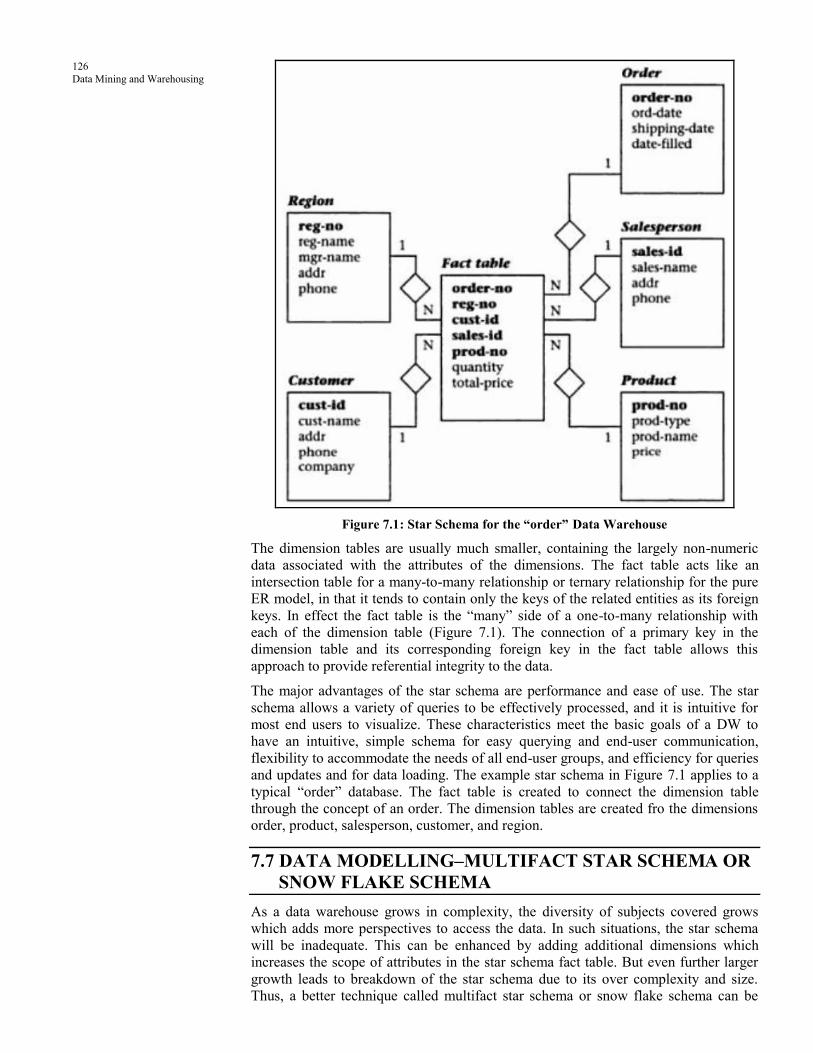
126


Figure 7.1: Star Schema for the “order” Data Warehouse

The dimension tables are usually much smaller, containing the largely non-numeric

data associated with the attributes of the dimensions. The fact table acts like an

intersection table for a many-to-many relationship or ternary relationship for the pure

ER model, in that it tends to contain only the keys of the related entities as its foreign

keys. In effect the fact table is the “many” side of a one-to-many relationship with

each of the dimension table (Figure 7.1). The connection of a primary key in the

dimension table and its corresponding foreign key in the fact table allows this

approach to provide referential integrity to the data.

The major advantages of the star schema are performance and ease of use. The star

schema allows a variety of queries to be effectively processed, and it is intuitive for

most end users to visualize. These characteristics meet the basic goals of a DW to

have an intuitive, simple schema for easy querying and end-user communication,

flexibility to accommodate the needs of all end-user groups, and efficiency for queries

and updates and for data loading. The example star schema in Figure 7.1 applies to a

typical “order” database. The fact table is created to connect the dimension table

through the concept of an order. The dimension tables are created fro the dimensions

order, product, salesperson, customer, and region.

7.7 DATA MODELLING–MULTIFACT STAR SCHEMA OR

SNOW FLAKE SCHEMA

As a data warehouse grows in complexity, the diversity of subjects covered grows

which adds more perspectives to access the data. In such situations, the star schema

will be inadequate. This can be enhanced by adding additional dimensions which

increases the scope of attributes in the star schema fact table. But even further larger

growth leads to breakdown of the star schema due to its over complexity and size.

Thus, a better technique called multifact star schema or snow flake schema can be

127

Data Warehouse utilized. The goal of this schema is to provide aggregation at different levels of

hierarchies in a given dimension. This goal is achieved by normalizing those

hierarchical dimensions into more detailed data sets to facilitate the aggregation of

fact data. It is possible to model the data warehouse into separate groups, where each

group addresses specific performance and trend analysis objective of a specific user.

Each group of fact data can be modeled using a separate star schema.

7.8 CATEGORIES OF OLAP TOOLS

OLAP tools can be broadly classified into two categories: MOLAP tools and ROLAP

tools. MOLAP tools presuppose the data to be present in a multidimensional database

(MDDB). In other words, data which has basically multidimensional nature, if loaded

into a multidimensional database, can be utilized by MOLAP tools for analysis. On

other hand, a typical relational database application (without MDDB) can be

processed by ROLAP (or relational OLAP) tools. However, there also exit hybrid

approaches which integrate both MOLAP and ROLAP techniques and they are

usually called multi-relational database systems. All these tools basically implement

‘star schema’ or ‘snowflake schema’, already discussed.

Applications of OLAP are being wide in range—both in business and government. In

business, the typical applications range from sales analysis, marketing campaigning,

sales forecasting and capacity planning. Similarly, in the government applications, we

can cite examples as commodity price monitoring, analysis and forecasting, plan

formulation, analysis and forecasting, agricultural production analysis and forecasting,

based on rainfall analysis, etc. The scope of application of these tools both in

government and business is almost unlimited, the spread of market between MOLAP

and ROLAP is as shown in Figure 7.2.

Figure 7.2: OLAP Comparison (The Area of Circles indicate the Data Size)

7.8.1 MOLAP

MOLAP-based products organize, navigate and analyze data typically in an

aggregated form. They require tight coupling with the applications and they depend

upon a multidimensional database (MDDB) system. Efficient implementations store

the data in a way similar to the form in which it is utilized by using improved storage

techniques so as to minimize storage. Many efficient techniques are used as spare data

storage management on disk so as to improve the response time. Some OLAP tools, as

Pilot products (Software Analysis Server) introduce ‘time’ also as an additional

dimension for analysis, thereby enabling time ‘series’ analysis. Some products as

Oracle Express Server introduce strong analytical capabilities into the database itself.

Applications requiring iterative and comprehensive time series analysis of trends are

well suited for MOLAP technology (e.g. financial analysis and budgeting). Examples

128


include Arbor Software’s Essbase. Oracle’s Express Server, Pilot Software’s

Lightship Server, Sinper’s TM/1. Planning Science’s Gentium and Kenan

Technology’s Multiway.

Some of the problems faced by users are related to maintaining support to multiple

subject areas in an RDBMS. As shown in Figure 7.3. these problems can be solved by

the some vendors by maintaining access from MOLAP tools to detailed data in and

RDBMS.

This can be very useful for organizations with performance-sensitive

multidimensional analysis requirements and that have built or are in the process of

building a data warehouse architecture that contains multiple subject areas. An

example would be the creation of sales data measured by several dimensions (e.g.

product and sales region) to be stored and maintained in a persistent structure. This

structure would be provided to reduce the application overhead of performing

calculations and building aggregation during initialization. These structures can be

automatically refreshed at predetermined intervals established by an administrator.

Figure 7.3: MOLAP Architecture

7.8.2 ROLAP

Relational OLAP (or ROLAP) is the latest and fastest growing OLAP technology

segment in the market. Many vendors have entered the fray in this direction (e.g.

Sagent Technology and Micro-strategy). By supporting a dictionary layer of metadata,

the RDBMS products have bypassed any requirement for creating a static,

multidimensional data structure as shown in Figure 7.4.

Figure 7.4: ROLAP Architecture

This approach enables multiple multidimensional views of two-dimensional relational

tables to be created, avoiding structuring data around the desired view. Some products

in this segment have supported strong SQL engines to support the complexity of

multidimensional analysis. This includes creating multiple SQL statements to handle

user requests, being ‘RDBMS’ aware’ and also being capable of generating the SQL

129

Data Warehouse statements based in the optimizer of the DBMS engine. While flexibility is the

attractive feature of ROLAP, there exist products which require the use of

denormalized database design. However, of late there is a noticeable change or

realignment in ROLAP technology. Firstly, there is a shift towards pure middle-ware

technology so as to simplify the development of multidimensional applications.

Secondly, the sharp delineation between ROLAP and other tools and RDBMS

products are now eager to provide multidimensional persistent structures with

facilities to assist in the administrations of these structures. Notable among vendors of

such products are micro-strategy (DSS Agent/DSS server), Platinium/Perodea

Software (Beacon), Information Advantage (AxSys), Informix/Stanford Technology

Group (Metacube) and SyBASE (HighGate Project).

7.8.3 Managed Query Environment (MQE)

Recent trend of OLPA is to enable capability for users to perform limited analysis

directly against RDBMS products or by bringing in an intermediate limited MOLAP

server.

Figure 7.5: Hybrid/MQE Architecture

Some vendor’s products have been able to provide ad hoc query as ‘data cube’ and

‘slice and dice’ analysis capabilities. This is achieved by first developing a query to

select data from the DBMS, which then delivers the requested data to the desktop

system where it is placed into a data cube. This data cube can be locally stored in the

desktop an also manipulated there so as to reduce the overhead required to create the

structure each time the query is executed. Once the data is placed in the data cube the

user can locally perform multidimensional analysis and also slice, dice and pivot

operations on it. In another approach, these tools can work with MOLAP servers, the

data from RDBMS can first go to MOLAP server and then to the desktop.

The ease of operation, administration and installation of such products makes them

particularly attractive to users who are familiar with simple RDBMS usage and

environment. This approach provides sophisticated analysis capabilities to such users

without significant costs involved in other more complex products in the market.

With all the ease of installation and administration that accompanies the desktop

OLAP products, most of these require the data cube to be built and maintained on the

desktop or a separate server along with metadata definitions that assist users in

retrieving the correct set of data that makes up the data cube. This method causes data

redundancy and strain to most network infrastructures that user to build a customize

data cube, the lack of data consistency among users, and the relatively small amount

of data that can be efficiently maintained are significant challenges facing all

administrators of these tools.

130



Write the full form of:

1. MOLAP …………………………………………………..

2. ROLAP …………………………………………………..

3. MQE …………………………………………………..

4. HOLAP …………………………………………………..

7.9 STATE OF THE MARKET

Overview of the state of the International Market:

Basically OLAP tools provide a more intuitive and analytical way to view corporate

or organizational data. These tools aggregate data along common subjects of business

or dimensions and then let users navigate through the hierarchies and dimensions with

the click of a mouse, users can drill down, across, or up across levels in each

dimension or pivot and swap out dimensions to change their view of the data. All this

can be achieved by various OLAP tools in the international market. Such free

manipulation of data provides insight into data, usually not possible by any other

means.

Some tools, such as Arbor Software Corp.’s Essbase and Oracle’s Ecpress, pre-

aggregate data into special multidimensional databases. Other tools work directly

against relational data and aggregate data on the fly, such as Micro-strategy Inc. DSS

Agent or Information Advantage Inc. Decision Suite. Some tools process OLAP data

on the desktop instead of a server. Desktopm OLAP tools include Cognos PowerPlay,

Brio Technology Inc. Brioquery, Planning Sciences Inc. Gentium and Andyne’s

Pablo. Many of the differences between OLAP tools are fading. Vendors are re-

architecting their products to give users greater control over the trade-off between

flexibility and performance that is inherent in OLAP tools. Many vendors have

rewritten their products in Java.

Eventually conventional database vendors may become the largest OLAP providers.

The leading database vendors incorporated OLAP functionality in their database

kernels. Oracle, Informix and also Microsoft have taken steps toward this end by

acquiring OLAP vendors (IRI Software, Standford Technology Group and Panorama,

respectively). As a result, the OLAP capabilities of their Group and DBMS products

are varying in their scope. Subsequently, IBM acquiring Informix along with all its

products.

Red Brick System’s Red Brick Ware tool’s for multidimensional analysis of corporate

data. PowerPlay, can be characterized as an MQE tool that can leverage corporate

investment in the relational database technology to provide multidimensional access

to enterprise data. PowerPlay also provides robustness, scalability and administrative

control.

7.9.1 Cognos PowerPlay

Cognos PowerPlay is an open OLAP solution that cam interface and interoperate with

a wise variety of third-party software tools, database and applications. The analytical

data used by PowerPlay is stored in multidimensional data sets called PowerCubes.

Cognos client/server architecture allows for the PowerCubes to be stored on the

Cognos universal client or on a server. PowerPlay offers a single universal client for

OLAP servers that support PowerCubes locally situated on the LAN or (optionally)

inside popular relational database. In addition to the fast installation and deployment

capabilities, PowerPlay provides a high level of usability with a familiar Windows

131

Data Warehouse interface, high performance, scalability, and relatively low cost of ownership.

Specifically, starting with version 5, Cognos PowerPlay client offers:

Support for enterprise-size data sets (PowerCubes) of 20+ million records,

100,000 categories and 100 measures.

A drill-through capability for queries from Cognos Impromptu Powerful 3-D

charting capabilities with background and rotation control for advanced users.

Scatter charts that let users show data across two measures, allowing easy

comparison of budget to actual values.

Linked displays that give users multiple views of the same data in report

Full support for OLE2 Automation, as both a client and a server

Formatting features for financial reports: brackets for negative numbers, single

and double underlining, and reverse sign for expenses.

Faster and easier ranking of data.

A ‘home’ button that automatically rests the dimension line to the top level.

Unlimited undo levels and customizable toolbars.

An enhanced PowerPlay portfolio that lets build graphical, interactive, EIS-type

briefing books from PowerPlay reports; Impromptu reports; word processing,

spreadsheet, or presentation documents; or any other documents or reports.

A 32-bit architecture for Windows NT, Windows 95/98

Access to third-party OLAP tools including direct native access to Arbor’s

Essbase and Oracle’s Express multidimensional databases.

PowerCube creation and access within existing relationship databases such as

Oracle, SyBASE, or Microsoft SQL server right inside the data warehouse.

PowerCube creation scheduled for off-peak processing, or sequential to other

processes.

Advanced security control by dimension, category and measure on the client, the

server or both.

Remote analysis where users pull subsets of information from the server down to

the client.

Complete integration with relational database security and data management

features.

An open API through OLE automation, allowing both server and client-based

PowerCubes to be accessed by Visual Basic applications, spreadsheets, and other

third-party tools and applications.

As mentioned earlier, PowerPlay’s capabilities include drill-to-detail using

Impromptu. Also, cubes can be built using data from multiple sources. For the

administrators who are responsible for creating multidimensional cubes, new

capabilities allow them to populate these PowerCubes inside popular relational

databases, and to do the processing off the desktop and on UNIX servers. To provide a

robust administration capabilities, Cognos offers a companion tool PowerPlay

administrator, which is available in database and server editions.

In PowerPlay administrator database edition, the administrator would continue to

model the cube and run the population of the cube process on the client platform. The

advantage is that data from multiple sources can now be used to generate a

PointerCube for the client and the actual PowerCube can be inside a relational

database. This means that existing database management tools and the database

132


administrator can be used to manage the business data, and a single delivery

mechanism can be employed for both application and OLAP processing. A

sophisticated security model is provided which in effect creates a ‘master’ cube to

service a variety of users. This is defines and controlled through an authenticator, also

included with PowerPlay.

The administrator server of PowerPlay lets users process the population of the cube on

a UNIX platform. An administrator uses client transformer to create a model, and

moves it to the UNIX server using the supplied software component called Powergrid.

The server transformer, once triggered, will create the PowerCube, and the only

prerequisite is that all data sources be accessible. Once completed, the resulting

PowerCube is copied or transferred to the client platform for subsequent PowerPlay

analysis by the user. The authenticator can be used to establish user database

passwords and locations can be known to the authenticator.

PowerPlay can be used effectively for generation of reports on any multidimensional

cube generated by other tools as Oracle Express, Plato, Visual DW of DB2.

PowerPlay supports clients on Windows 3.1, 95, 98 and NT. Administrator database

and server editions execute on HP/UX, IBM AIX,a dn Sun Solaris, and support

PowerCubes in Oracle, Sybase SQL server, and Microsoft SQL server.

Latest Cognos PowerPlay release version 6 has Web-enabled features so as to present

the reports on the Web in 3-tier undirected use.

7.9.2 IBI Focus Fusion

Focus Fusion from Information Builders Inc (IBI) is a multidimensional database

technology for OLAP and data warehousing. It is designed to address business

applications that require multidimensional analysis of detail product data. Focus

Fusion complements Cactus and EDA/SQL middleware software to provide a

multifaceted data warehouse solution.

Focus Fusion combines a parallel-enabled, high-performance, multi-dimensional

database engine with the administrative, copy management and access tools,

necessary for a data warehouse solution designed specifically for deployment of

business intelligence applications in data warehouse environments, Fusion provides:

Fast query and reporting. Fusion’s advances indexing, parallel query, and roll-up

facilities provide high performance for reports, queries and analysis, with the

scalability users need to complete data warehouse solutions.

Comprehensive, graphics-based administration facilities that make Fusion

database applications easy to build and deploy.

Integrated copy management facilities, which schedule automatic data refresh

from any source into Fusion.

A complete portfolio of tightly integrated business intelligence applications that

span reporting, query decision support and EIS needs.

Open access via industry-standard protocols like ANSI SQL, ODBC and HTTP

via EDA/SQL, so that Fusion works with a wide variety of desktop tools,

including World Wide Web browsers.

Three-tiered reporting architecture for high performance

Scalability of OLAP applications form the department to the enterprise.

Access to precalculated summaries (roll-up)combined with dynamic detail data

manipulation capabilities.

Capability to perform intelligent application portioning without disrupting users.

133

Data Warehouse Interoperability with the leading EIS, DSS and OLAP tools.

Support for parallel computing environment.

Seamless integration with more than 60 different database engines on more than

35 platforms, including Oracle, Sybase, SAP, Hogon, Microsoft SQL server,

DB2. IMS and VSAM.

Focus Fusion’s proprietary OverLAP technology allows Fusion to serve as an OLAP

front-end or shared cache for relational and legacy databases, effectively providing a

virtual warehousing environment for the analysis of corporate data. This can simplify

warehouse management and lower overall costs by potentially reducing the need to

copy infrequently accessed detail data to the warehouse for a possible drill-down.

Focus Fusion is a modular tool that supports flexible configurations for diverse needs,

and includes the following components:

Fusion/DBserver: High-performance, client/server, parallel-enabled, scalable

multidimensional DBMS. Fucion/Dbserver runs on both UNIX and NT and

connects transparently to all enterprise data that EDA/SQL can access.

Fusion/Dbserver also provides stored procedure and remote procedure call (RPC)

facilities.

Fusion/Administrator: Comprehensive GUI-based (Windows) administration

utility that provides visual schema definition and bulk load of Fusion databases,

multidimensional index definition and build, and rollup definition and creation.

Additionally, Fusion/Administrator automates migration of FOCUS databases to

Fusion.

Fusion/PDQ: Parallel data query for Fusion/Dbserver exploits symmetric

multiprocessor (SMP) hardware for fast query execution and parallel loads.

EDA.Link: Fusion’s client component supports standard API’s, including ODBC

and ANSI SQL, EDA/Link provides access to Fusion from any desktop (Windows

95/NT, UNIX, Macintosh, OS/2) or host system (UNIX, MVS, AS400, VMS,

etc.) over TCP/IP and many other network topologies (via EDA Hub servers) to

integrate Fusion’s products into enterprise processes.

EDA/WebLink: Fusion’s open browser client that supports Netscape, Mosaic

Internet Explorer, and all other standard HTML browsers. It works with

Information Builders HTML generator to facilitate Web-based warehouse

publishing applications.

Enterprise Copy Manger for Fusion: Fully automated assembly, transformation,

summarization, and load of enterprise data from any source into Fusion on

schedule basis. It consists of Enterprise Copy Server, Enterprise Copy Client (the

graphical Windows-based interface), and Enterprise Source Server (the remote

gateway access to source data).

EDA Gateways: Remote data access gateways that provide transparent, live drill

through capabilities from Fusion/DBserver to production databases.

7.9.3 Pilot Software

Pilot Software offers the Pilot Decision Support of tools from a high speed

multidimensional database (MOLAP), data warehouse integration (ROLAP), data

mining, and a diverse set of customizable business applications targeted after sales

and marketing professionals. The following products are at the core of Pilot

Software’s offering:

Pilot Analysis Server: A full-function multidimensional database with high-speed

consolidation, graphical user interface (Pilot Model Builder), and expert-level

interface. The latest version includes relational integration of the

134


multidimensional model with relational data stores, thus allowing the user the

choice between high-speed access of a multidimensional database of on-the-fly

(ROLAP) access of detail data stored directly in the warehouse or data mart.

Pilot Link: A database connectivity tool that includes ODBC connectivity and

high-speed connectivity via specialized drivers to the most popular relational

database platforms. A graphical user interface allows the user seamless and easy

access to a wide variety of distributed databases.

Pilot Designer: An application design environment specifically created to enable

rapid development of OLAP applications.

Pilot Desktop: A collection of applications that allows the end-user easy

navigation and visualization of the multidimensional database.

Pilot Sales and Marketing Analysis Library: A collection of sophisticated

applications designed for the sales and marketing business end-user. The

applications can be modified and tailored to meet individual needs for particular

customers.

Pilot Discovery Server: A predictive data mining tool that embeds directly into

the relational database and does not require the user to copy or transform the data.

The data mining result are stored with metadata into the data warehouse as a

predictive segmentation and are embedded into the graphical user interface called

Pilot Discovery Launch, which helps building data mining models.

Pilot Internet Publisher: A tool that easily allows users to access their Pilot

multidimensional database via browser on the Internet or Intranets.

Some of the distinguishing features of Pilot’s product offering include the overall

complete solution from powerful OLAP engine and data mining engine to that

customizable business applications. Within their OLAP offering, some of the key

features of Pilot’s products are as under:

Time intelligence: The Pilot Analysis Server has a number of features to support

time as a special dimension. Among these are the ability to process data on the fly

to convert the native periodicity (e.g. the data collected weekly) to the periodicity

preferred by the customer viewing the data (e.g. view the data monthly). This

feature is accomplished via special optimized structures within the

multidimensional database.

Embedded data mining: The Pilot Analysis Server is the first product to integrate

predictive data mining with the multidimensional (as it is des model). This allows

the user to benefit not only from the predictive power of data mining but also

from the descriptive and analytical power of multidimensional navigation.

Multidimensional database compression: In addition to the compression of

sparsity, Pilot Analysis Server also has special code for compressing data values

over time. A new feature called a ‘dynamic dimension’ allows some dimensions

to be calculated on the fly when they are attributes of an existing dimension. This

allows the (as it is des to be much smaller and still provide fast access. Dynamic

variables which are also calculated on the fly are also available to further decrease

the total size of the database and thus decrease the time for consolidation of the

database.

Relational integration: Pilot allows for a seamless integration of both MOLAP

and ROLAP to provide the user with either the speed of MOLAP or the more

space-efficient ROLAP. The users interface with the system, by defining the

multidimensional model or view that prefer, and the system self-optimizes the

queries.

135

Data Warehouse 7.9.4 Arbor Essbase Web

Essbase is one of the most ambitious of the early Web products. It includes not only

OLAP manipulations, such as drill up down and across, pivot, slice and dice; and

fixed dynamic reporting but also data entry, including full multi-user concurrent write

capabilities—a feature that differentiates it from the others.

Arbor sells Essbase only as a server, it does not have a client package. The Web

product does not replace administrative and development modules; only user can

access it for query and update.

7.9.5 Information Advantage Web OLAP

Information Advantage uses a server-centric message architecture, which is composes

of a powerful analytical engine that generate SQL. It also pulls data from relational

databases, manipulates the results and transfers the results to a client.

Since all the intelligence of the product is in the server implementing Web OLAP to

provide a Web-based client is straightforward, the architecture of Information

Advantage’s Web product is similar to that of Essbase with a Web gateway between

the Web server and the analytical engine. Although in this case, data store and an

analytical engine are separate, Essbase is both data store and analytical engine.

7.9.6 Microstrategy DSS Web

Microstrategy’s DSS Agent originally a Windows-only tool, but now it is also OLAP

tools to have a Web-access product. DSS along with DSS server relational OLAP

server—DSS architect data modeling tools, and DSS executive design tool for

building Executive Information Systems—generates SQL dynamically and relies on

the relational database server to perform complex analysis, rather than creating a

‘cube’ like most of the other tools. By inserting a Web gateway between the Web

server and the DSS server engine, Microstrategy was able to replace the interactive

DSS agent front-end with a Web browser, which passes requests to the DSS server’s

API.

7.9.7 Brio Technology

Brio offers a suite of products called Brio.web.warehouse. This suite implements

several of the approaches listed above for deploying decision support OLAP

applications on the web. The key to Brio’s strategy are new server components called

Brio.quickview and Brio.insight which can off load processing from the clients and

thus enable users to access Brio reports via Web browsers. On the client side, Brio

uses plug-ins to give users viewing and manipulation capabilities.

For these and other reasons the web is a perfect medium for decision support. The

general features of the Web-enabled data access are as under:

The first-generation Web sites used a static distribution model, in which clients

access static HTML pages via Web browsers. In this model, the decision support

reports are stored as HTML documents and are delivered to users on request.

Clearly, this model has some serious deficiencies, including inability to provide

Web clients with dynamic updates and interactive analytical capabilities such as

drill-down.

The second-generation Web sites support interactive and dynamic database by

utilizing a multi-tiered architecture in which a Web client submits a query in the

form of HTML-encoded request to a Web server, which in turn transforms the

request for structured data into a Common Gateway Interface (CGI) script, or a

script written to a proprietary Web-server API. The gateway submits SQL queries

to the database, receives the result, translates them into HTML and sends the

pages to the requester. Requests for the unstructured data (e.g. images, other

136


HTML documents, etc.) can be sent directly to the unstructured data store, pre-

calculated MOLAP storage or directly in the relational data store depending on

the usage pattern and the time/space trade-off preferences of the end-user.

7.10 OLAP TOOLS AND THE INTERNET

The Web technologies indeed are the natural choice for adaptation for data

warehousing. The internet is virtually a free resource which provides a universal

connectivity within and between companies and also individuals.

Some of the web facilities are as under:

The Web eases complex administrative tasks of managing distributed

environments.

The Web allows companies to store and manage both data and applications on

servers that can be centrally managed and updated, thus eliminating problems

with software and data accuracy.

The emerging third-generation Web sites replace HTML gateways with Web

based application servers. These servers can download Java applets or ActiveX

applications that execute on clients, or interact with corresponding applets running

on servers-servlets. The third-generation Web servers provide users with all the

capabilities of existing decision-support applications without requiring them to

load any client software except a Web browser.

Not surprisingly, vendors of decision support applications, especially query, reporting

and OLAP tools, are rapidly converting their tools to work on the Web. Vendor

approaches for deploying tools on the Web include the following:

HTML publishing: This approach involves transforming an output of a query into

the HTML page that can be downloaded into browser. This approach does not

support interactive access to data or reports.

Helper applications: In this approach a tool is configured as a helper application

that resides within a browser. This is the case of a ‘fat’ client, in which, once the

data is downloaded, users can take advantage of all capabilities of the tool to

analyse data. However, maintaining these helper applications becomes another

task for system administrator.

Plug-ins: A variation on the previous approach, plug-ins are helper applications

that are downloaded from the server prior to their initial use. Since the plug-ins

are downloaded from the server, their normal administration and installation tasks

are significantly reduced. However, typically, plug-ins are browser-specific and

may not run on all platforms or with all browsers. Also, as browsers get updated,

these plug-ins may have to be upgraded as well, creating additional administration

workload.

Server-centric components: In this approach, the vendor rebuilds a desktop tool

as a server component, or creates a new server component that can be integrated

with the Web via a Web gateway (e.g. CGI or NSAPI scripts).

Java and ActiveX applications: This approach is for a vendor to redevelop all or

portions of its tool in Java or ActiveX. The result is a true ‘thin’ client model.

Despite some disadvantages, this approach appears to be one of the most

promising and flexible.

137

Data Warehouse The following are some of the Web-based tools:

Arbor Essbase Web: This tool offers features as drilling up, down, across; slice

and dice and dynamic reporting, all for OLAP. It also offers data entry, including

full multi-user concurrent write capabilities.

Arbor Essbase is only a server product, no client package exists, thus protecting

its own desktop client version market. The Web product does not replace

administrative and development modules but it replaces only user access for query

and update.

Information Advantage Web OLAP: This product uses a server centric

messaging architecture, composed of a powerful analytic engine which generate

SQL for the retrieval from relational database, manipulate the results and transfer

the results into a client.

Since it is all server-centric capability, implementing Web OLAP to provide web-

based client is easy and simple. This architecture is similar to the one of Essbase

with a Web gateway between Web server and analytic engine, even though the

data store and the engine are separate.

Microstrategy DSS Web: The flagship product DSS Agent from Microstrategy,

originally a Window tool, is now available on all platforms and also on the Web.

DSS Agent, along with the complement product—DSS server relational OLAP

server, DSS Architect data-modelling tools, the DSS Executive design tool for

building executive information system (EIS), generate SQL automatically and

dynamically. It depends on the RDBMS server for performing complex analysis,

instead of creating a multidimensional ‘Cube’. Then it is offering ROLAP and not

MOLAP. By inserting a Web Gateway between the Web server and DSS server

engine, Microstrategy is replacing the interactive DSS Agent front-end with a web

browser which passes through it in terms of request to DSS server API.

Brio technology: Brio released ;brio.web.warehouse; suits of products in the end

of 1998. most of the Web OLAP approaches described earlier are available in this

suite. A new server component called ‘brio.query.server’ works in tandem with

Brio Enterprise Web-clients ‘brio-quickview’ and ‘brio.insight’ and enable Web

access by browsers.

7.11 LET US SUM UP

All OLAP vendors position their products to be fully Web compliant. The scope of

functionality and a particular style of implementation will become a market

differentiator for these tools.

Server-centric tools, such as Information Advantage abd Prodea Beacon from

Platinum Technology and the multidimensional OLAP tools—Arbor’s Essbase Orable

Express, Planning Science Gentia, Kenan Technologies Acumate Es, Holistic Systems

Holos, and Pilot Software’s Pilot Server—appear to be in an excellent position to take

advantage of their architecture to provide easy access from a Web browser. Similarly,

client-centric tools such as Business Objects, Software Ags Esperant, Cognos

PowerPlay or Brio Technologies, Brio suit of products, are making available robust

and full-featured Web-enabled versions of their products. The tasks become easier as

both Java and ActiveX are available for the Web deployment.


Discuss the characteristics of data warehousing.

138


7.13 KEYWORDS

A data warehouse: It is a relational database that is designed for query and analysis

rather than for transaction processing.

A data warehouse architecture: It is a description of the elements and services of the

warehouse, with details showing how the components will fit together and how the

system will grow over time.

Job control: This includes job definition, job scheduling (time and event), monitoring,

logging, exception handling, error handling, and notification.


1. How a date warehouse is different from data base? Explain with the help of

suitable example.

2. Highlights the main differences between OLTP and Data warehouse.

3. Explain the architecture of Data Warehouse in details.

4. Describe the criteria for a Data Warehouse DBMS Selection.

5. What could be the strategy to design a data warehouse architecture? Discuss.


CYP 1

1. The logical link between what the managers see in their decision support

EIS applications and the company’s operational activities.

2. A data mart is a collection of subject areas organized for decision support

based on the needs of a given department. Finance has their data mart,

marketing has theirs, sales has theirs and so on. And the data mart for

marketing only faintly resembles anyone else’s data mart.

CYP 2

1. Multidimensional Online Analytical Processing

2. Relational Online Analytical Online Analytical Process

3. Managed Query Environment

4. Hybrid Online Analytical Processing


Usama Fayyad, “Mining Databases: Towards Algorithms for Knowledge Discovery”, Bulletin

of the IEEE Computer Society Technical Committee on Data Engineering, vol. 21, no. 1,

March 1998.

Christopher Matheus, Philip Chan, and Gregory Piatetsky-Shapiro, “Systems for Knowledge

Discovery in Databases”, IEEE Transactions on Knowledge and Data Engineering, 5(6):903-

913, December 1993.

Rakesh Agrawal and Tomasz Imielinski, “Database Mining: A Performance Perspective”,

IEEE Transactions on Knowledge and Data Engineering, 5(6):914-925, December 1993.

Usama Fayyad, David Haussler, and Paul Stolorz, “Mining Scientific Data”, Communications

of the ACM, vol. 39, no. 11, pp. 51-57, November 1996.

David J. Hand, “Data Mining: Statistics and more?”, The American Statistician, vol. 52, no. 2,

pp 112-118, May 1998.

139

Data Warehouse

Tom M. Mitchell, “Does machine learning really work?”, AI Magazine, vol. 18, no. 3, pp. 11-

20, Fall 1997.

Clark Glymour, David Madigan, Daryl Pregibon, and Padhraic Smyth, “Statistical Inference

and Data Mining”, Communications of the ACM, vol. 39, no. 11, pp. 35-41, November 1996.

Hillol Kargupta, Ilker Hamzaoglu, and Brian Stafford, “Scalable, Distributed Data Mining

using An Agent Based Architecture”, Proceedings of the Third International Conference on

Knowledge Discovery and Data Mining (KDD-97), August 1997, Newport Beach, California,

USA.

M-S. Chen, Jiawei Han, and Philip S. Yu, “Data Mining: An Overview from a Database

Perspective”, IEEE Transactions on Knowledge and Data Engineering, 8(6): 866-883, 1996.

Surajit Chaudhuri, “Data Mining and Database Systems: Where is the Intersection?”, Bulletin

of the IEEE Computer Society Technical Committee on Data Engineering, vol. 21, no. 1,

March 1998.

140


LESSON

8 DATA WAREHOUSE AND OLAP TECHNOLOGY

CONTENTS


8.1 Introduction

8.2 What is a Data Warehouse?

8.2.1 Use of Data Warehouses in Organisations

8.2.2 Differences between Operational Database Systems and Data Warehouses

8.2.3 Need to Build a Data Warehouse

8.3 A Multi-Dimensional Data Model

8.3.1 Relational Implementation of the Model

8.3.2 OLAP Operations in the Multi-dimensional Data Model

8.4 Data Warehouse Architecture

8.4.1 Process of Data Warehouse Design

8.4.2 Data Warehouse Models

8.4.3 OLAP Server Architectures

8.5 Further Development of Data Cube Technology

8.6 Let us Sum up


8.8 Keywords





The concept of data warehouse

Basic knowledge of OLAP Technology

8.1 INTRODUCTION

This lesson is an introduction to data warehouses and OLAP (On-Line Analytical

Processing). Topics include the concept of data warehouses and multi-dimensional

databases, the construction of data cubes, the implementation of on-line analytical

processing, and the relationship between data warehousing and data mining.

8.2 WHAT IS A DATA WAREHOUSE?

Data warehouse provides architectures and tools for business executives to

systematically organise, understand, and use their data to make strategic decisions.

141

Data Warehouse and

OLAP Technology

In the last several years, many firms have spent millions of dollars in building

enterprise-wide data warehouses as it is assumed a way to keep customers by learning

more about their needs.

In simple terms, a data warehouse refers to a database that is maintained separately

from an organisation's operational databases. Data warehouse systems allow for the

integration of a variety of application systems. They support information processing

by providing a solid platform of consolidated, historical data for analysis.

According to W.H. Inman, a leading architect in the construction of data warehouse

systems, "a data warehouse is a subject-oriented, integrated, time-variant, and

nonvolatile collection of data in support of management's decision making process."

The four keywords, subject-oriented, integrated, time-variant, and non-volatile,

distinguish data warehouses from other data repository systems, such as relational

database systems, transaction processing systems, and file systems. Let us understand

the four keywords in more detail as follows:

Subject-oriented: A data warehouse focuses on the modeling and analysis of data

for decision makers. Therefore, data warehouses typically provide a simple and

concise view around particular subject issues by excluding data that are not useful

in the decision support process. For example, a typical data warehouse is

organised around major subjects, such as customer, vendor, product, and sales

rather than concentrating on the day-to-day operations and transaction processing

of an organisation.

Integrated: As the data warehouse is usually constructed by integrating multiple

heterogeneous sources, such as relational databases, flat files, and on-line

transaction records, the data cleaning and data integration techniques need to be

applied to ensure consistency in naming conventions, encoding structures,

attribute measures, and so on.

Time-variant: Data are stored to provide information from a historical perspective

(e.g., the past 5-10 years). Every key structure in the data warehouse contains,

either implicitly or explicitly, an element of time.

Non-volatile: A data warehouse is always a physically separate store of data

transformed from the application data found in the operational environment. Due

to this separation, a data warehouse does not require transaction processing,

recovery, and concurrency control mechanisms. It usually requires only two

operations in data accessing: initial loading of data and access of data.

8.2.1 Use of Data Warehouses in Organisations

Many organisations are creating data warehouse to support business decision-making

activities for the following reasons:

To increasing customer focus, which includes the analysis of customer buying

patterns (such as buying preference, buying time, budget cycles, and appetites for

spending),

To reposition products and managing product portfolios by comparing the

performance of sales by quarter, by year, and by geographic regions, in order to

fine-tune production strategies,

To analysing operations and looking for sources of profit, and

To managing the customer relationships, making environmental corrections, and

managing the cost of corporate assets,

Data warehousing is also very useful from the point of view of heterogeneous

database integration. Many organisations typically collect diverse kinds of data

and maintain large databases from multiple, heterogeneous, autonomous, and

distributed information sources.

142


Query Driven Approach versus Update Driven Approach for Heterogeneous

Database Integration

For heterogeneous database integration, the traditional database implements query-

driven approach, which requires complex information filtering and integration

processes, and competes for resources with processing at local sources. It is inefficient

and potentially expensive for frequent queries, especially for queries requiring

aggregations.

In query-driven approach, data warehousing employs an update-driven approach in

which information from multiple, heterogeneous sources is integrated in advance and

stored in a warehouse for direct querying and analysis. In this approach, a data

warehouse brings high performance to the integrated heterogeneous database system

since data are copied, preprocessed, integrated, annotated, summarised, and

restructured into one semantic data store. Furthermore, query processing in data

warehouses does not interfere with the processing at local sources. Moreover, data

warehouses can store and integrate historical information and support complex

multidimensional queries. As a result, data warehousing has become very popular in

industry.

8.2.2 Differences between Operational Database Systems and Data

Warehouses

The first major stepping stone in understanding Data Warehousing is to grasp the

concepts and differences between the two overall database categories. The type most

of us are used to dealing with is the On Line Transactional Processing (OLTP)

category. The other major category is On Line Analytical Processing (OLAP).

OLTP is what we characterise as the ongoing day-to-day functional copy of the

database. It is where data is added and updated but never overwritten or deleted. The

main needs of the OLTP operational database being easily controlled insertion and

updating of data with efficient access to data manipulation and viewing mechanisms.

Typically only single record or small record-sets should be manipulated in a single

operation in an OLTP designed database. The main thrust here is to avoid having the

same data in different tables. This basic tenet of Relational Database modeling is

known as “normalising” data.

OLAP is a broad term that also encompasses data warehousing. In this model data is

stored in a format, which enables the efficient creation of data mining/reports. OLAP

design should accommodate reporting on very large record sets with little degradation

in operational efficiency. The overall term used to describe taking data structures in an

OLTP format and holding the same data in an OLAP format is “Dimensional

Modeling”. It is the primary building block of Data Warehousing.

The major distinguishing features between OLTP and OLAP are summarised as

follows:

Feature OLTP System OLAP System

Characteristic Operational Processing Informational Processing

Users Clerks, clients, and information

technology professionals.

Knowledge workers, including

managers, executives, and analysts.

System orientation Customer oriented and used for

transaction and query processing Day to day operations

Market-oriented and used for data

analysis long-term informational requirements, decision support.

Data contents Manages current data that typically,

are too detailed to be easily used for

decision making.

Manages large amounts of

historical data, provides facilities

for summarisation and aggregation,

and stores and manages information at different levels of granularity.

Contd….

143

Data Warehouse and

OLAP Technology

Database design Adopts an entity-relationship (ER)

data model and an application- oriented database design

Adopts either a star or snowflake

model and a subject-oriented database design.

View Focuses mainly on the current data

within an enterprise or department,

without referring to historical data or data in different organisations.

In contrast, an OLAP system often

spans multiple versions of a

database schema, due to the

evolutionary process of an

organisation. OLAP systems also

deal with information that

originates from different

organisations, integrating

information from many data

stores.

Volume of data Not very large Because of their huge volume,

OLAP data are stored on multiple storage media.

Access patterns Consists mainly of short, atomic

transactions. Such a system requires

concurrency control and recovery mechanisms.

Accesses to OLAP systems are

mostly read-only operations (since

most data warehouses store

historical rather than up-to-date

information), although many could be complex queries.

Access mode Read/write Mostly write

Focus Data in Information out

Operations Index/hash on primary key Lots of scans

Number of records

accessed

Tens Millions

Number of users Thousands Hundreds

DB size 100 MB to GB 100 GB to TB

Priority High performance, high availability High flexibility, end-user

autonomy

Metric Transaction throughput Query response time

8.2.3 Need to Build a Data Warehouse

You know that data warehouse queries are often complex. They involve the

computation of large groups of data at summarised levels and may require the use of

special data organisation, access, and implementation methods based on

multidimensional views. Processing OLAP queries in operational databases would

substantially degrade the performance of operational tasks. Moreover, an operational

database supports the concurrent processing of several transactions as well recovery

mechanism such as locking and logging to ensure the consistency and robustness of

transactions. An OLAP query often needs read-only access of data records for

summarisation and aggregation. Concurrency control and recovery mechanisms, if

applied for such OLAP operations, may jeopardise the execution of concurrent

transactions and thus substantially reduce the throughput of an OLTP system.



…………………………………..………………………………………….

…………………………………..………………………………………….

2. Why are many organisations creating data warehouses to support business

activities?

…………………………………..………………………………………….

…………………………………..………………………………………….

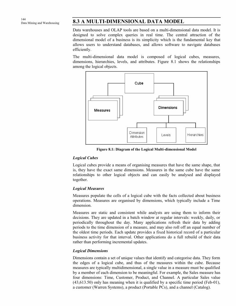
144


8.3 A MULTI-DIMENSIONAL DATA MODEL

Data warehouses and OLAP tools are based on a multi-dimensional data model. It is

designed to solve complex queries in real time. The central attraction of the

dimensional model of a business is its simplicity which is the fundamental key that

allows users to understand databases, and allows software to navigate databases

efficiently.

The multi-dimensional data model is composed of logical cubes, measures,

dimensions, hierarchies, levels, and attributes. Figure 8.1 shows the relationships

among the logical objects.

Figure 8.1: Diagram of the Logical Multi-dimensional Model

Logical Cubes

Logical cubes provide a means of organising measures that have the same shape, that

is, they have the exact same dimensions. Measures in the same cube have the same

relationships to other logical objects and can easily be analysed and displayed

together.

Logical Measures

Measures populate the cells of a logical cube with the facts collected about business

operations. Measures are organised by dimensions, which typically include a Time

dimension.

Measures are static and consistent while analysts are using them to inform their

decisions. They are updated in a batch window at regular intervals: weekly, daily, or

periodically throughout the day. Many applications refresh their data by adding

periods to the time dimension of a measure, and may also roll off an equal number of

the oldest time periods. Each update provides a fixed historical record of a particular

business activity for that interval. Other applications do a full rebuild of their data

rather than performing incremental updates.

Logical Dimensions

Dimensions contain a set of unique values that identify and categorise data. They form

the edges of a logical cube, and thus of the measures within the cube. Because

measures are typically multidimensional, a single value in a measure must be qualified

by a member of each dimension to be meaningful. For example, the Sales measure has

four dimensions: Time, Customer, Product, and Channel. A particular Sales value

(43,613.50) only has meaning when it is qualified by a specific time period (Feb-01),

a customer (Warren Systems), a product (Portable PCs), and a channel (Catalog).

145

Data Warehouse and

OLAP Technology

Logical Hierarchies and Levels

A hierarchy is a way to organise data at different levels of aggregation. In viewing

data, analysts use dimension hierarchies to recognise trends at one level, drill down to

lower levels to identify reasons for these trends, and roll up to higher levels to see

what affect these trends have on a larger sector of the business.

Each level represents a position in the hierarchy. Each level above the base (or most

detailed) level contains aggregate values for the levels below it. The members at

different levels have a one-to-many parent-child relation. For example, Q1-2002 and

Q2-2002 are the children of 2002, thus 2002 is the parent of Q1-2002 and Q2-2002.

Suppose a data warehouse contains snapshots of data taken three times a day, that is,

every 8 hours. Analysts might normally prefer to view the data that has been

aggregated into days, weeks, quarters, or years. Thus, the Time dimension needs a

hierarchy with at least five levels.

Similarly, a sales manager with a particular target for the upcoming year might want

to allocate that target amount among the sales representatives in his territory; the

allocation requires a dimension hierarchy in which individual sales representatives are

the child values of a particular territory.

Hierarchies and levels have a many-to-many relationship. A hierarchy typically

contains several levels, and a single level can be included in more than one hierarchy

Logical Attributes

An attribute provides additional information about the data. Some attributes are used

for display. For example, you might have a product dimension that uses Stock

Keeping Units (SKUs) for dimension members. The SKUs are an excellent way of

uniquely identifying thousands of products, but are meaningless to most people if they

are used to label the data in a report or graph. You would define attributes for the

descriptive labels.

Multi-dimensional Data Storage in Analytic Workspaces:

In the logical multidimensional model, a cube represents all measures with the same

shape, that is, the exact same dimensions. In a cube shape, each edge represents a

dimension. The dimension members are aligned on the edges and divide the cube

shape into cells in which data values are stored.

In an analytic workspace, the cube shape also represents the physical storage of

multidimensional measures, in contrast with two-dimensional relational tables. An

advantage of the cube shape is that it can be rotated: there is no one right way to

manipulate or view the data. This is an important part of multidimensional data

storage, calculation, and display, because different analysts need to view the data in

different ways. For example, if you are the Sales Manager, then you need to look at

the data differently from a product manager or a financial analyst.

Assume that a company collects data on sales. The company maintains records

that quantify how many of each product was sold in a particular sales region during

a specific time period. You can visualise the sales measure as the cube shown in

Figure 8.2.

146


Figure 8.2: Comparison of Product Sales by City

Figure 8.2 compares the sales of various products in different cities for January 2001

(shown) and February 2001 (not shown). This view of the data might be used to

identify products that are performing poorly in certain markets. Figure 8.3 shows sales

of various products during a four-month period in Rome (shown) and Tokyo (not

shown). This view of the data is the basis for trend analysis.

Figure 8.3: Comparison of Product Sales by Month

A cube shape is three dimensional. Of course, measures can have many more than

three dimensions, but three dimensions are the maximum number that can be

represented pictorially. Additional dimensions are pictured with additional cube

shapes.

8.3.1 Relational Implementation of the Model

The relational implementation of the multi-dimensional data model is typically a star

schema, as shown in Figure 8.4, a snowflake schema or a fact constellation schema.

Star Schema: A star schema is a convention for organising the data into dimension

tables, fact tables, and materialised views. Ultimately, all of the data is stored in

columns, and metadata is required to identify the columns that function as

multidimensional objects.

147

Data Warehouse and

OLAP Technology

Figure 8.4: Diagram of a Star Schema

(a) Dimension Tables: A star schema stores all of the information about a dimension

in a single table. Each level of a hierarchy is represented by a column or column

set in the dimension table. A dimension object can be used to define the

hierarchical relationship between two columns (or column sets) that represent two

levels of a hierarchy; without a dimension object, the hierarchical relationships are

defined only in metadata. Attributes are stored in columns of the dimension tables.

A snowflake schema normalises the dimension members by storing each level in a

separate table.

(b) Fact Tables: Measures are stored in fact tables. Fact tables contain a composite

primary key, which is composed of several foreign keys (one for each dimension

table) and a column for each measure that uses these dimensions.

(c) Materialised Views: Aggregate data is calculated on the basis of the hierarchical

relationships defined in the dimension tables. These aggregates are stored in

separate tables, called summary tables or materialised views. Oracle provides

extensive support for materialised views, including automatic refresh and query

rewrite.

Queries can be written either against a fact table or against a materialised view. If a

query is written against the fact table that requires aggregate data for its result set, the

query is either redirected by query rewrite to an existing materialised view, or the data

is aggregated on the fly.

Each materialised view is specific to a particular combination of levels; in Figure 8.5,

only two materialised views are shown of a possible 27 (3 dimensions with 3 levels

have 3**3 possible level combinations).

148


Example:

Let, an organisation sells products throughtout the world. The main four major

dimensions are product, location, time and organisation.

Figure 8.5: Example of Star Schema

In the example Figure 8.5, sales fact table is connected to dimensions location,

product, time and organisation. It shows that data can be sliced across all dimensions

and again it is possible for the data to be aggregated across multiple dimensions.

"Sales Dollar" in sales fact table can be calculated across all dimensions

independently or in a combined manner, which is explained below:

Sales Dollar value for a particular product

Sales Dollar value for a product in a location

Sales Dollar value for a product in a year within a location

Sales Dollar value for a product in a year within a location sold or serviced by an

employee

Snowflake Schema: The snowflake schema is a variant of the star schema model,

where some dimension tables are normalised, thereby further splitting the data into

additional tables. The resulting schema graph forms a shape similar to a snowflake.

The major difference between the snowflake and star schema models is that the

dimension tables of the snowflake model may be kept in normalised form. Such a

table is easy to maintain and also saves storage space because a large dimension table

can be extremely large when the dimensional structure is included as columns. Since

much of this space is redundant data, creating a normalised structure will reduce the

overall space requirement. However, the snowflake structure can reduce the

effectiveness of browsing since more joins will be needed to execute a query.

Consequently, the system performance may be adversely impacted. Performance

benchmarking can be used to determine what is best for your design.

Example:

In Snowflake schema, the example diagram shown in Figure 8.6 has 4 dimension

tables, 4 lookup tables and 1 fact table. The reason is that hierarchies (category,

branch, state, and month) are being broken out of the dimension tables (PRODUCT,

ORGANISATION, LOCATION, and TIME) respectively and shown separately. In

OLAP, this Snowflake schema approach increases the number of joins and poor

performance in retrieval of data.

149

Data Warehouse and

OLAP Technology

Figure 8.6: Example of Snowflake Schema

A compromise between the star schema and the snowflake schema is to adopt a mixed

schema where only the very large dimension tables are normalised. Normalising large

dimension tables saves storage space, while keeping small dimension tables

unnormalised may reduce the cost and performance degradation due to joins on

multiple dimension tables. Doing both may lead to an overall performance gain.

However, careful performance tuning could be required to determine which dimension

tables should be normalised and split into multiple tables.

Fact Constellation: Sophisticated applications may require multiple fact tables to

share dimension tables. This kind of schema can be viewed as a collection of stars,

and hence is called a galaxy schema or a fact constellation. For example, A fact

constellation schema of a data warehouse for sales and shipping is shown in the

following Figure 8.7.

Figure 8.7: Fact Constellation Schema of a Data Warehouse for Sales and Shipping

150


Difference between a Data Warehouse and a Data Mart

In data warehousing, there is a distinction between a data warehouse and a data mart.

A data warehouse collects information about subjects that span the entire organisation,

such as customers, items, sales, assets, and personnel, and thus its scope is enterprise-

wide. For data warehouses, the fact constellation schema is commonly used since it

can model multiple, interrelated subjects. A data mart, on the other hand, is a

department subset of the data warehouse that focuses on selected subjects, and thus its

scope is department-wide. For data marts, the star or snowflake schema are popular

since each are geared towards modeling single subjects

Introducing Concept Hierarchies

A concept hierarchy defines a sequence of mappings from a set of low level concepts

to higher level, more general concepts. Consider a concept hierarchy for the

dimension location. City values for location include Lucknow, Mumbai, New York,

and Chicago. Each city, however, can be mapped to the province or state to which it

belongs. For example, Lucknow can be mapped to Uttar Pradesh, and Chicago to

Illinois. The provinces and states can in turn be mapped to the country to which they

belong, such as India or the USA. These mappings form a concept hierarchy for the

dimension location, mapping a set of low level concepts (i.e., cities) to higher level,

more general concepts (i.e., countries). The concept hierarchy described above is

illustrated in Figure 8.8.

Figure 8.8: Example of Concept Hierarchy

Many concept hierarchies are implicit within the database schema. For example,

suppose that the dimension location is described by the attributes number, street, city,

province-or_state, zipcode, and country. These attributes are related by a total order,

forming a concept hierarchy such as "street < city < province.or.state < country". This

hierarchy is shown in Figure 8.9(a).

(a) a hierarchy for location (b) a lattice for time

Figure 8.9: Hierarchical and Lattice Structures of Attributes in Warehouse Dimensions

151

Data Warehouse and

OLAP Technology

Alternatively, the attributes of a dimension may be organised in a partial order,

forming a lattice. An example of a partial order for the time dimension based on the

attributes day, week, month, quarter, and year is "day < month <quarter; week <

year". This lattice structure is shown in Figure 8.9(b).

A concept hierarchy that is a total or partial order among attributes in a database

schema is called a schema hierarchy. Concept hierarchies that are common to many

applications may be predefined in the data mining system, such as the concept

hierarchy for time. Data mining systems should provide users with the flexibility to

tailor predefined hierarchies according to their particular needs. For example, one may

like to define a fiscal year starting on April 1, or an academic year starting on

September 1.


Explain the difference between a data warehouse and a data mart.

……………………………………..…………………………………………...

……………………………………..…………………………………………...

8.3.2 OLAP Operations in the Multi-dimensional Data Model

Data Warehouses use On-line Analytical Processing (OLAP) to formulate and execute

user queries. OLAP is an SLQ-based methodology that provides aggregate data

(measurements) along a set of dimensions, in which each dimension table includes a

set of attributes each measure depends on a set of dimensions that provide context for

the measure, e.g. for the reseller company, the measure is the number of sold units,

which are described by the corresponding location, time, and item type all dimensions

are assumed to uniquely determine the measure, e.g., for the reseller company, the

location, time, producer, and item type provide all necessary information to determine

context of a particular number of sold units.

There are five basic OLAP commands that are used to perform data retrieval from a

Data warehouse.

1. ROLL UP, which is used to navigate to lower levels of details for a given data

cube. This command takes the current data cube (object) and performs a GROUP

BY on one of the dimensions, e.g., given the total number of sold units by month,

it can provide sales summarised by quarter.

2. DRILL DOWN, which is used to navigate to higher levels of detail. This

command is the opposite of ROLL UP, e.g., given the total number of units sold

for an entire continent, it can provide sales in the U.S.A.

3. SLICE, which provides a cut through a given data cube. This command enables

users to focus on some specific slice of data inside the cube, e.g., the user may

want to look at the data concerning unit sales only in Mumbai.

4. DICE, which provides just one cell from the cube (the smallest slice), e.g. it can

provide data concerning the number of sold Canon printers in May 2002 in

Lucknow.

5. PIVOT, which rotates the cube to change the perspective, e.g., the “time item”

perspective may be changed into “time location.”

These commands, in terms of their specification and execution, are usually carried out

using a point-and-click interface, and therefore we do not describe their syntax.

Instead, we give examples for each of the above OLAP commands.

ROLL UP Command

The ROLL UP allows the user to summarise data into a more general level in

hierarchy. For instance, if the user currently analyses the number of sold CPU units

152


for each month in the first half of 2002, this command will allows him/her to

aggregate this information into the first two quarters. Using ROLL UP, the view

Figure 8.10: Example ROLL UP Command

is transformed into

From the perspective of a three-dimensional cuboid, the time _y_ axis is transformed

from months to quarters; see the shaded cells in Figure 8.10.

DRILL DOWN Command

The DRILL DOWN command provides a more detailed breakdown of information

from lower in the hierarchy. For instance, if the user currently analyses the number of

sold CPU and Printer units in Europe and U.S.A., it will allows him/her to find details

of sales in specific cities in the U.S.A., i.e., the view.

is transformed into

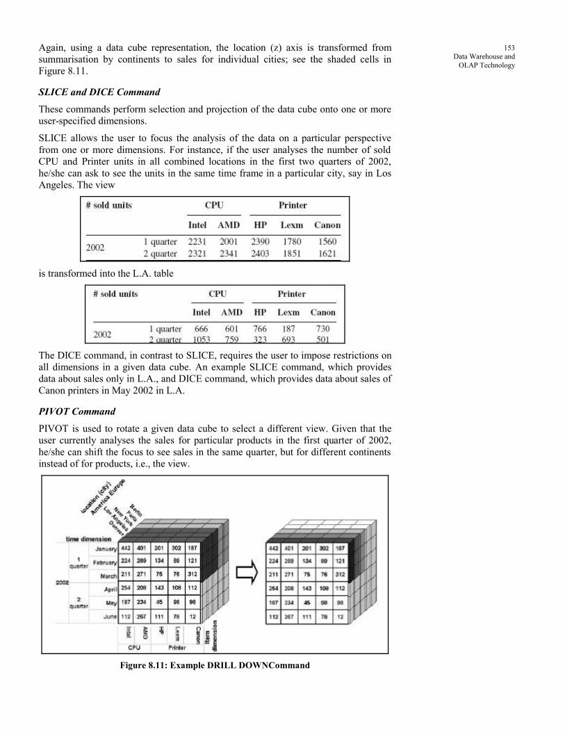
153

Data Warehouse and

OLAP Technology

Again, using a data cube representation, the location (z) axis is transformed from

summarisation by continents to sales for individual cities; see the shaded cells in

Figure 8.11.

SLICE and DICE Command

These commands perform selection and projection of the data cube onto one or more

user-specified dimensions.

SLICE allows the user to focus the analysis of the data on a particular perspective

from one or more dimensions. For instance, if the user analyses the number of sold

CPU and Printer units in all combined locations in the first two quarters of 2002,

he/she can ask to see the units in the same time frame in a particular city, say in Los

Angeles. The view

is transformed into the L.A. table

The DICE command, in contrast to SLICE, requires the user to impose restrictions on

all dimensions in a given data cube. An example SLICE command, which provides

data about sales only in L.A., and DICE command, which provides data about sales of

Canon printers in May 2002 in L.A.

PIVOT Command

PIVOT is used to rotate a given data cube to select a different view. Given that the

user currently analyses the sales for particular products in the first quarter of 2002,

he/she can shift the focus to see sales in the same quarter, but for different continents

instead of for products, i.e., the view.

Figure 8.11: Example DRILL DOWNCommand

154


is transformed into

8.4 DATA WAREHOUSE ARCHITECTURE

Why do Business Analysts Need Data Warehouse?

A data warehouse is a repository of an organisation's electronically stored data. Data

warehouses are designed to facilitate reporting and analysis. It provides many

advantages to business analysts as follows:

A data warehouse may provide a competitive advantage by presenting relevant

information from which to measure performance and make critical adjustments in

order to help win over competitors.

A data warehouse can enhance business productivity since it is able to quickly and

efficiently gather information, which accurately describes the organisation.

A data warehouse facilitates customer relationship marketing since it provides a

consistent view of customers and items across all lines of business, all

departments, and all markets.

A data warehouse may bring about cost reduction by tracking trends, patterns, and

exceptions over long periods of time in a consistent and reliable manner.

A data warehouse provides a common data model for all data of interest,

regardless of the data's source. This makes it easier to report and analyse

information than it would be if multiple data models from disparate sources were

used to retrieve information such as sales invoices, order receipts, general ledger

charges, etc.

Because they are separate from operational systems, data warehouses provide

retrieval of data without slowing down operational systems.

8.4.1 Process of Data Warehouse Design

A data warehouse can be built using three approaches:

A top-down approach

A bottom-up approach

A combination of both approaches

The top-down approach starts with the overall design and planning. It is useful in

cases where the technology is mature and well-known, and where the business

problems that must be solved are clear and well-understood.

The bottom-up approach starts with experiments and prototypes. This is useful in the

early stage of business modeling and technology development. It allows an

organisation to move forward at considerably less expense and to evaluate the benefits

of the technology before making significant commitments.

In the combined approach, an organisation can exploit the planned and strategic nature

of the top-down approach while retaining the rapid implementation and opportunistic

application of the bottom-up approach.

155

Data Warehouse and

OLAP Technology

In general, the warehouse design process consists of the following steps:

Choose a business process to model, e.g., orders, invoices, shipments, inventory,

account administration, sales, and the general ledger. If the business process is

organisational and involves multiple, complex object collections, a data

warehouse model should be followed. However, if the process is departmental and

focuses on the analysis of one kind of business process, a data mart model should

be chosen.

Choose the grain of the business process. The grain is the fundamental, atomic

level of data to be represented in the fact table for this process, e.g., individual

transactions, individual daily snapshots, etc.

Choose the dimensions that will apply to each fact table record. Typical

dimensions are time, item, customer, supplier, warehouse, transaction type, and

status.

Choose the measures that will populate each fact table record. Typical measures

are numeric additive quantities like dollars-sold and units-sold.

Once a data warehouse is designed and constructed, the initial deployment of the

warehouse includes initial installation, rollout planning, training and orientation.

Platform upgrades and maintenance must also be considered. Data warehouse

administration will include data refreshment, data source synchronisation, planning

for disaster recovery, managing access control and security, managing data growth,

managing database performance, and data warehouse enhancement and extension.

Figure 8.12: A Three-tier Data Warehousing Architecture

156


A Three-tier Data Warehouse Architecture:

Data Warehouses generally have a three-level (tier) architecture that includes:

A bottom tier that consists of the Data Warehouse server, which is almost always

a RDBMS. It may include several specialised data marts and a metadata

repository,

A middle tier that consists of an OLAP server for fast querying of the data

warehouse. The OLAP server is typically implemented using either (1) a

Relational OLAP (ROLAP) model, i.e., an extended relational DBMS that maps

operations on multidimensional data to standard relational operations; or (2) a

Multidimensional OLAP (MOLAP) model, i.e., a special purpose server that

directly implements multidimensional data and operations.

A top tier that includes front-end tools for displaying results provided by OLAP,

as well as additional tools for data mining of the OLAP-generated data.

The overall DW architecture is shown in Figure 8.12.

8.4.2 Data Warehouse Models

From the architecture point of view, there are three data warehouse models: the virtual

warehouse, the data mart, and the enterprise warehouse.

Virtual Warehouse: A virtual warehouse is created based on a set of views defined

for an operational RDBMS. This warehouse type is relatively easy to build but

requires excess computational capacity of the underlying operational database system.

The users directly access operational data via middleware tools. This architecture is

feasible only if queries are posed infrequently, and usually is used as a temporary

solution until a permanent data warehouse is developed.

Data Mart: The data mart contains a subset of the organisation-wide data that is of

value to a small group of users, e.g., marketing or customer service. This is usually a

precursor (and/or a successor) of the actual data warehouse, which differs with respect

to the scope that is confined to a specific group of users.

Depending on the source of data, data marts can be categorised into the following two

classes:

Independent data marts are sourced from data captured from one or more

operational systems or external information providers, or from data generated

locally within a particular department or geographic area.

Dependent data marts are sourced directly from enterprise data warehouses.

Enterprise warehouse: This warehouse type holds all information about subjects

spanning the entire organisation. For a medium- to a large-size company, usually

several years are needed to design and build the enterprise warehouse.

The differences between the virtual and the enterprise DWs are shown in Figure 8.13.

Data marts can also be created as successors of an enterprise data warehouse. In this

case, the DW consists of an enterprise warehouse and (several) data marts.

157

Data Warehouse and

OLAP Technology

Figure 8.13: A Virtual Data Warehouse and an Enterprise Data Warehouse

8.4.3 OLAP Server Architectures

We describe here the physical implementation of an OLAP server in a Data

Warehouse. There are three different possible designs:

Relational OLAP (ROLAP)

Multidimensional OLAP (MOLAP)

Hybrid OLAP (HOLAP)

ROLAP

ROLAP stores the data based on the already familiar relational DBMS technology. In

this case, data and the related aggregations are stored in RDBMS, and OLAP

middleware is used to implement handling and exploration of data cubes. This

architecture focuses on the optimisation of the RDBMS back end and provides

additional tools and services such as data cube navigation logic. Due to the use of the

RDBMS back end, the main advantage of ROLAP is scalability in handling large data

volumes. Example ROLAP engines include the commercial IBM Informix Metacube

(www.ibm.com) and the Micro-strategy DSS server (www.microstrategy.com), as

well as the open-source product Mondrian (mondrian.sourceforge.net).

MOLAP

In contrast to ROLAP, which uses tuples as the data storage unit, the MOLAP uses a

dedicated n-dimensional array storage engine and OLAP middleware to manage data.

Therefore, OLAP queries are realised through a direct addressing to the related

multidimensional views (data cubes). Additionally, this architecture focuses on pre-

calculation of the transactional data into the aggregations, which results in fast query

158


execution performance. More specifically, MOLAP precalculates and stores

aggregated measures at every hierarchy level at load time, and stores and indexes

these values for immediate retrieval. The full precalculation requires a substantial

amount of overhead, both in processing time and in storage space. For sparse data,

MOLAP uses sparse matrix compression algorithms to improve storage utilisation,

and thus in general is characterised by smaller on-disk size of data in comparison with

data stored in RDBMS. Example MOLAP products are the commercial Hyperion

Ebasse (www.hyperion.com) and the Applix TM1 (www.applix.com), as well as Palo

(www.opensourceolap.org), which is an open-source product.

HOLAP

To achieve a tradeoff between ROLAP’s scalability and MOLAP’s query

performance, many commercial OLAP servers are based on the HOLAP approach. In

this case, the user decides which portion of the data to store in the MOLAP and which

in the ROLAP. For instance, often the low-level data are stored using a relational

database, while higher-level data, such as aggregations, are stored in a separate

MOLAP. An example product that supports all three architectures is Microsoft’s

OLAP Services (www.microsoft.com/), which is part of the company’s SQL Server.


What are the approaches of data warehouse design?

……………………………………..…………………………………………...

……………………………………..…………………………………………...

8.5 FURTHER DEVELOPMENT OF DATA CUBE

TECHNOLOGY

On-Line Analytical Processing (OLAP) characterises the operations of summarising,

consolidating, viewing, applying formulae to, and synthesising data along multiple

dimensions. OLAP software helps analysts and managers gain insight into the

performance of an enterprise through a wide variety of views of data organised to

reflect the multi-dimensional nature of enterprise data. An increasingly popular data

model for OLAP applications is the multi-dimensional database, also known as the

data cube.

Hypothesis-driven Exploration

A user or analyst can search for interesting patterns in the cube by specifying a

number of OLAP operations, such as drill-down, roll-up, slice, and dice. While these

tools are available to help the user explore the data, the discovery process is not

automated. It is the user who, following her own intuition or hypotheses, tries to

recognise exceptions or anomalies in the data. This hypothesis-driven exploration has

a number of disadvantages. The search space can be very large, making manual

inspection of the data a daunting and overwhelming task. High-level aggregations

may give no indication of anomalies at lower levels, making it easy to overlook

interesting patterns. Even when looking at a subset of the cube, such as a slice, the

user is typically faced with many data values to examine. The sheer volume of data

values alone makes it easy for users to miss exceptions in the data if using hypothesis-

driven exploration.

Discovery-driven Exploration of Data Cubes

A new discovery-driven method of data exploration overcomes the anomalies of

hypothesis-driven exploration. In this method, analyst's search for anomalies is guided

by precomputed indicators of exceptions at various levels of detail in the cube. This

increases the chances of user noticing abnormal patterns in the data at any level of

aggregation.

159

Data Warehouse and

OLAP Technology

Intuitively, an exception is a data cube cell value that is significantly different from

the value anticipated, based on a statistical model. The model considers variations and

patterns in the measure value across all of the dimensions to which a cell belongs. For

example, if the analysis of item-sales data reveals an increase in sales in December in

comparison to all other months, this may seem like an exception in the time

dimension. However, it is not an exception if the item dimension is considered, since

there is a similar increase in sales for other items during December. The model

considers exceptions hidden at all aggregated group-by's of a data cube. Visual cues

such as background color are used to reflect the degree of exception of each cell,

based on the precomputed exception indicators. The computation of exception

indicators can be overlapped with cube construction, so that the overall construction

of data cubes for discovery-driven exploration is efficient.

Three measures are used as exception indicators to help identify data anomalies.

These measures indicate the degree of surprise that the quantity in a cell holds, with

respect to its expected value. The measures are computed and associated with every

cell, for all levels of aggregation. They are:

SelfExp: This indicates the degree of surprise of the cell value, relative to other

cells at the same level of aggregation.

InExp: This indicates the degree of surprise somewhere beneath the cell, if we

were to drill down from it.

PathExp: This indicates the degree of surprise for each drill-down path from the

cell.

The use of these measures for discovery-driven exploration of data cubes is illustrated

in the following example.

Example:

Consider a user looking at the monthly sales as a percentage difference from the

previous month. Suppose the user starts by viewing the data aggregated over all

products and markets for different months of the year as shown in Figure.

To find out what parts of the cube may be worthy of exploring further in terms of

exceptions, the user invokes a “highlight exceptions" button that colors the

background of each cell based on its SelfExp value. In addition, each cell is

surrounded with a different colored box based on the InExp value. In both cases, the

intensity of the color is varied with the degree of exception. In Figure 2.14, the

months with a thick box around them have a high InExp value and thus need to be

drilled down further for exceptions underneath them. Darker boxes (e.g., around

“Aug”, “Sep” and “Oct”) indicate higher values of InExp than the lighter boxes (e.g.,

around “Feb” and “Nov”).

There are two paths the user may drill down along from here: Product and Region. To

evaluate which of these paths has more exceptions, the user selects a cell of interest

and invokes a “path exception" module that colors each aggregated dimension based

on the surprise value along that path. These are based on the PathExp values of the

cell. In Figure 8.14 (top-left part) the path along dimension Product has more surprise

than along Region indicated by darker color.

Drilling-down along Product yields 143 different sales values corresponding to

different Product-Time combinations as shown in Figure 8.14.

160


Figure 8.14: Change in Sales Over Time for each Product

Instead of trying to find the exceptions by manual inspection, the user can click on the

“highlight exception" button to quickly identify the exceptional values. In this figure

there are a few cells with high SelfExp values and these appear as cells with a

different background shade than the normal ones (darker shades indicate higher

surprise). For instance, sales of “Birch-B(eer)" shows an exceptional difference of

42% in the month of “Oct". In addition, three other cells are also indicated to have

large SelfExp values although the sales values themselves ( 6% for <Jolt-C, Sep>,

-12% for <Birch-B, Jul> and -10% for <Birch-B, Dec>) are not exceptionally large

when compared with all the other cells.

Figure 8.14 also shows some cells with large InExp values as indicated by the thick

boxes around them. The highest InExp values are for Product “Diet-Soda” in the

months of “Aug” and “Oct”. The user may therefore choose to explore further details

for “Diet-Soda” by drilling down along Region. Figure 8.15 shows the sales figures

for “Diet-Soda” in different Regions. By highlighting exceptions in this plane, the

user notices that in Region “E" (for Eastern), the sales of “Diet-Soda” has decreased

by an exceptionally high value of 40% and 33% in the months of “Aug” and “Oct”

respectively. Notice that the sales of “Diet-Soda” in the Product-Time plane

aggregated over different Regions (Figure 8.15) gives little indication of these high

exceptions in the Region-Product-Time space. This shows how the InExp value at

higher level cells may be valuable in reaching at exceptions in lower level cells.

Figure 8.15: Change in Sales of Product “Diet-Soda” Over Time in each Region

There are no other cells with high InExp in Figure 8.15. Therefore, the user may stop

drilling down and go back to the Product-Time plane of Figure 8.14 to explore other

cells with high InExp. Suppose, he chooses to drill-down along Product “Cola” in

“Aug”. Figure 8.16 shows the exceptions for “Cola" after drilling down along Region.

The “Central” Region has a large InExp and may be drilled down further, revealing

the SelfExp values in the Market-time plane for “Cola”.

161

Data Warehouse and

OLAP Technology

Figure 8.16: Change in Sales Over Time for Product “Cola" in different Region

Defining Exceptions

The SelfExp, InExp, and PathExp measures are based on a statistical method for table

analysis. They take into account all of the group-by (aggregations) in which a given

cell value participates. A cell value is considered an exception based on how much it

differs from its expected value, where its expected value is determined with a

statistical model described below. The difference between a given cell value and its

expected value is called a residual. Intuitively, the larger the residual, the more the

given cell value is an exception. The comparison of residual values requires us to

scale the values based on the expected standard deviation associated with the

residuals. A cell value is therefore considered an exception if its scaled residual value

exceeds a pre-specified threshold. The SelfExp, InExp, and PathExp measures are

based on this scaled residual.

Complex Aggregation at Multiple Granularities: Multifeature Cubes

Data cubes facilitate the answering of data mining queries as they allow the

computation of aggregate data at multiple levels of granularity. Multifeature cubes

compute complex queries involving multiple dependent aggregates at multiple

granularities. These cubes are very useful in practice. Many complex data mining

queries can be answered by multifeature cubes without any significant increase in

computational cost, in comparison to cube computation for simple queries with

standard data cubes.


Fill in the blanks:

1. In query-driven approach, data warehousing employs an ………………..

approach in which information from multiple, heterogeneous sources is

integrated in advance and stored in a warehouse for direct querying and

analysis.

2. Data warehouses and ……………….. tools are based on a

multidimensional data model.

3. Logical cubes provide a means of organising measures that have the same

shape, that is, they have the exact same ……………….. .

4. A ……………….. schema stores all of the information about a dimension

in a single table.

5. The ……………….. schema is a variant of the star schema model, where

some dimension tables are normalised, thereby further splitting the data

into additional tables.

8.6 LET US SUM UP

A data warehouse is a subject-oriented, integrated, time-variant, and nonvolatile

collection of data organised in support of management decision making. Several

factors distinguish data warehouses from operational databases. Since the two systems

162


provide quite different functionalities and require different kinds of data, it is

necessary to maintain data warehouses separately from operational databases.

A multidimensional data model is typically used for the design of corporate data

warehouses and departmental data marts. Such a model can adopt either a star schema,

snowflake schema, or fact constellation schema. The core of the multidimensional

model is the data cube, which consists of a large set of facts (or measures) and a

number of dimensions. Dimensions are the entities or perspectives with respect to

which an organisation wants to keep records, and are hierarchical in nature. Concept

hierarchies organise the values of attributes or dimensions into gradual levels of

abstraction. They are useful in mining at multiple levels of abstraction. On-Line

Analytical Processing (OLAP) can be performed in data warehouses/ marts using the

multidimensional data model. Typical OLAP operations include roll-up, drill-(down,

cross, through), slice-and-dice, pivot (rotate), as well as statistical operations such as

ranking, computing moving averages and growth rates, etc. OLAP operations can be

implemented efficiently using the data cube structure. Data warehouses often adopt a

three-tier architecture. The bottom tier is a warehouse database server, which is

typically a relational database system. The middle tier is an OLAP server, and the top

tier is a client, containing query and reporting tools.

OLAP servers may use Relational OLAP (ROLAP), or Multidimensional OLAP

(MOLAP), or Hybrid OLAP (HOLAP). A ROLAP server uses an extended relational

DBMS that maps OLAP operations on multi-dimensional data to standard relational

operations. A MOLAP server maps multi-dimensional data views directly to array

structures. A HOLAP server combines ROLAP and MOLAP. For example, it may use

ROLAP for historical data while maintaining frequently accessed data in a separate

MOLAP store.


Discuss difference between OLTP system and OLAP system. Also discuss the

concept of snowflake schema.

8.8 KEYWORDS

Data warehouse: A data warehouse is a subject-oriented, integrated, time-variant, and

nonvolatile collection of data in support of management’s decision making process.

OLTP: On Line Transactional Processing.

OLAP: On Line Analytical Processing.

Logical Cubes: Logical cubes provide a means of organising measures that have the

same shape, that is, they have the exact same dimensions.

Logical Measures: Measures populate the cells of a logical cube with the facts

collected about business operations. Measures are organised by dimensions, which

typically include a Time dimension.

Logical Dimensions: Dimensions contain a set of unique values that identify and

categorise data. They form the edges of a logical cube, and thus of the measures

within the cube.

Logical Hierarchies: A hierarchy is a way to organise data at different levels of

aggregation.

Star Schema: A star schema is a convention for organising the data into dimension

tables, fact tables, and materialised views.

Snowflake Schema: The snowflake schema is a variant of the star schema model,

where some dimension tables are normalised, thereby further splitting the data into

additional tables.

163

Data Warehouse and

OLAP Technology

Concept Hierarchy: A concept hierarchy defines a sequence of mappings from a set

of low level concepts to higher level, more general concepts.

ROLL UP: It is used to navigate to lower levels of details for a given data cube.

DRILL DOWN: It is used to navigate to higher levels of detail.

SLICE: It provides a cut through a given data cube.

DICE: It provides just one cell from the cube.

PIVOT: It rotates the cube to change the perspective, e.g., the “time item” perspective

may be changed into “time location.”

Relational OLAP (ROLAP) model: It is an extended relational DBMS that maps

operations on multidimensional data to standard relational operations.

Multidimensional OLAP (MOLAP) model: It is a special purpose server that directly

implements multidimensional data and operations.

Virtual warehouse: A virtual warehouse is created based on a set of views defined for

an operational RDBMS.


1. Explain the concept of concept hierarchy.

2. Explain five basic OLAP commands that are used to perform data retrieval from a

Data warehouse.

3. What is the process of designing a data warehouse?

4. Draw the figure of 3-tier data warehouse.

5. Explain the difference between a data mart and a data warehouse.

6. Differentiate between the ROLAP, MOLAP and HOLAP.

7. Write a short note on “Further development of data cube technology.”


CYP 1

1. A data warehouse refers to a database that is maintained separately from

an organisation’s operational databases.

2. Many organisations are creating data warehouse to support business

decision-making activities for the following reasons:

To increasing customer focus, which includes the analysis of

customer buying patterns (such as buying preference, buying time,

budget cycles, and appetites for spending),

To reposition products and managing product portfolios by

comparing the performance of sales by quarter, by year, and by

geographic regions, in order to fine-tune production strategies,

To analysing operations and looking for sources of profit, and

To managing the customer relationships, making environmental

corrections, and managing the cost of corporate assets.

Contd….

164


CYP 2

In data warehousing, there is a distinction between a data warehouse and a

data mart. A data warehouse collects information about subjects that span the

entire organisation, such as customers, items, sales, assets, and personnel, and

thus its scope is enterprise-wide. For data warehouses, the fact constellation

schema is commonly used since it can model multiple, interrelated subjects. A

data mart, on the other hand, is a department subset of the data warehouse that

focuses on selected subjects, and thus its scope is department-wide. For data

marts, the star or snowflake schema are popular since each are geared towards

modeling single subjects.

CYP 3

A data warehouse can be built using three approaches:

1. a top-down approach

2. a bottom-up approach

3. a combination of both approaches

CYP 4

1. Update-driven

2. OLAP

3. Dimensions

4. Star

5. Snowflake





1993.












Edition, 2004.


Publications, 2004.




Edition, 2000.

165

Developing Data

Warehouse

UNIT V

166


167

Developing Data

Warehouse

LESSON

9 DEVELOPING DATA WAREHOUSE

CONTENTS


9.1 Introduction

9.2 Why and How to Build a Data Warehouse

9.3 Date Warehouse Architectural Strategies and Organisational Issues

9.4 Design Considerations

9.5 Data Content

9.6 Metadata

9.7 Comparison of Data Warehouse and Operational Data

9.8 Distribution of Data

9.9 Tools for Data Warehousing

9.10 Performance Considerations

9.11 Crucial Decision in Designing a Data Warehouse

9.12 Let us Sum up


9.14 Keywords





The concept of warehouse development

Basic knowledge of warehouse architectural strategies

Organizational issues-design consideration

Data contents

9.1 INTRODUCTION

A fundamental concept of a data warehouse is the distinction between data and

information. Data is composed of observable and recordable facts that are often found

in operational or transactional systems. At Rutgers, these systems include the

registrar’s data on students (widely known as the SRDB), human resource and payroll

databases, course scheduling data, and data on financial aid. In a data warehouse

environment, data only comes to have value to end-users when it is organized and

presented as information. Information is an integrated collection of facts and is used

as the basis for decision-making. For example, an academic unit needs to have

diachronic information about its extent of instructional output of its different faculty

members to gauge if it is becoming more or less reliant on part-time faculty.

168


9.2 WHY AND HOW TO BUILD A DATA WAREHOUSE

Changes are taking place in the world continuously in all forms of activity. From a

business perspective, the quest for survival in a globally competitive environment has

become extremely demanding for all.

Business strategy requires answers to questions in business policy and future strategy.

This means that the decisions are required to be taken quickly and correctly using all

the available data. As the data size increases continuously, doubling every 18 months,

the speed requirements for processing this data so as to comprehend the meaning of

this data are also required to be increased significantly. Competition also adds

pressure on this situation and herein business intelligence becomes the foundation for

successful business strategy.

Here the need for data warehousing technology arises, in terms of ability to organize,

maintain large data and also be able to analyze in a few seconds in the manner and

depth as required.

Why did the conventional information systems not succeed in meeting these

requirements? Actually the conventional information systems and data warehousing

tackle two different activity domains—OLTP and OLAP. These domains are not at all

competitive with each other, they deal with two different problem domain

requirements. Further, as the technology upgrades, the CPU time and disk space are

growing larger and are becoming cheaper with time. Similarly, network bandwidths

are increasing and becoming cheaper day-by-day. Need for more and more

heterogeneity and interoperability is increasingly being felt. In this scenario, data

warehousing emerges as a promising technology.

In the following sections, we shall survey all the major issues involved in building a

data warehouse such as approach architectural strategy design considerations, data

content related issues, meta-data, distribution of data, tools and performance

considerations.

9.3 DATE WAREHOUSE ARCHITECTURAL STRATEGIES

AND ORGANISATIONAL ISSUES

A data warehouse can be built either on a top-down or on a bottom-up approach. In

other words, one can be define a global data warehouse for an entire organization and

split it up into individual data marts or sub data warehouses dedicated for individual

departments. Alternatively individual data marts can be built for each department and

then they all get finally integrated into a central data warehouse.

The bottom-up approach is more realistic but the integration of individual data marts

should be made easier with advanced planning and preparation.

All organizations active in information systems area are fully conversant with the

issues relating to information system implementation. But the issues pertaining to data

warehousing activity are quite different and divergent from these ones. In building a

data warehouse, the organization has to make arrangements for information flow from

various internal information systems and databases as well as from internal sources of

information. This requires close involvement of the users in identifying the

information requirements and identifying the sources of the same from both internal

and external data sources and information system in time.

9.4 DESIGN CONSIDERATIONS

The first and foremost design consideration is to be exhaustive and so to say holistic,

i.e. to exhaustively cover all possible data sources for exhaustively designing a data

warehouse with all possible components as part of a single complex system so as to

169

Developing Data

Warehouse

effectively meet all possible user requirements. Any failure in this regard may lead to

a data warehouse design that is skewed towards a particular requirement (missing

other requirements) or a particular data source, missing some other data sources or

oriented towards a particular access tool, thereby limiting its usage and accessibility.

Web enablement may subsequently enhance the data accessibility and its usage.

There are three major issues that will be faced in data warehouse development:

heterogeneity of data sources requiring substantial efforts in data conversion and also

in maintaining timeliness and high-quality levels of data integrity, reliability and

authenticity. Further, the data may be quite old and historical. While old data of past is

essential for a data warehouse, it should be ensured that it will be relevant and useful

in the data warehouse form. If any data is too old to be relevant any more it may not

be worthwhile to enter into the data warehouse. Another issue is the tendency of the

data warehouse to grow very large. Discrete decisions should be made by the designer

of the data warehouse in limiting the size of the warehouse by discretely dropping old

data and selecting appropriate data to be included into the warehouse.

The data warehouse design is distinctly different from regular OLTP based

information system design in many ways. Data warehouse design is business driven,

i.e. it is based on specific business goals to be achieved by the OLPA on the data

warehouse. In the case of OLTP systems, the design is driven by the existing

information system concerned. Since data warehouse design is business driven, it may

never be fully completed as the user’s business requirements and also data sources

keep changing. Keeping them in view the designer may be cautions in data warehouse

design so as to avoid the possible pitfalls.

9.5 DATA CONTENT

In what way does the data content in the warehouse differ from OLTP system? It is

normally misunderstood that data warehouse contains lesser level of detailed data

when compared on an OLTP system which may be its source. This is incorrect. The

level of detail of data in the data warehouse is normally the same as that of the source

OLTP system; only it may be in a different format. Typically, a data source contains

detail level data. But the data is cleaned and transferred to fit in the data warehouse

model.

The cleaning up process removes the deficiencies and loopholes in the data. In

addition, all the aspects related to transaction processing also will be filtered off

before putting into the warehouse, as they are not relevant in OLAP applications of

the warehouse.

The data model used in the data warehouse reflects the nature, content and structure of

the data in the warehouse. The data model represents the framework of the

organization and structure of the data in the data warehouse. The data model also

identifies how the information is stored in the data warehouse. It identifies major

subjects and relationship of the model, including keys, attributes and attribute

groupings.

In addition to the data model, the designer should also be able to identify the querying

process on the warehouse. Due to their broad scope and powerful nature, queries can

also determine the data model. The data model should be optimized so as to meet high

level query performance in terms of broad scope and analytical intensity. In addition,

data would also have a bearing on the data storage requirements and the data loading

performance.

As already discussed, the data model for the data warehouse may be quite different

from the data model for a data mart depending on the requirements of design of the

data marts vis-a-vis the data warehouse. The start schema and snowflake schema are

the most commonly used data models in data warehousing.

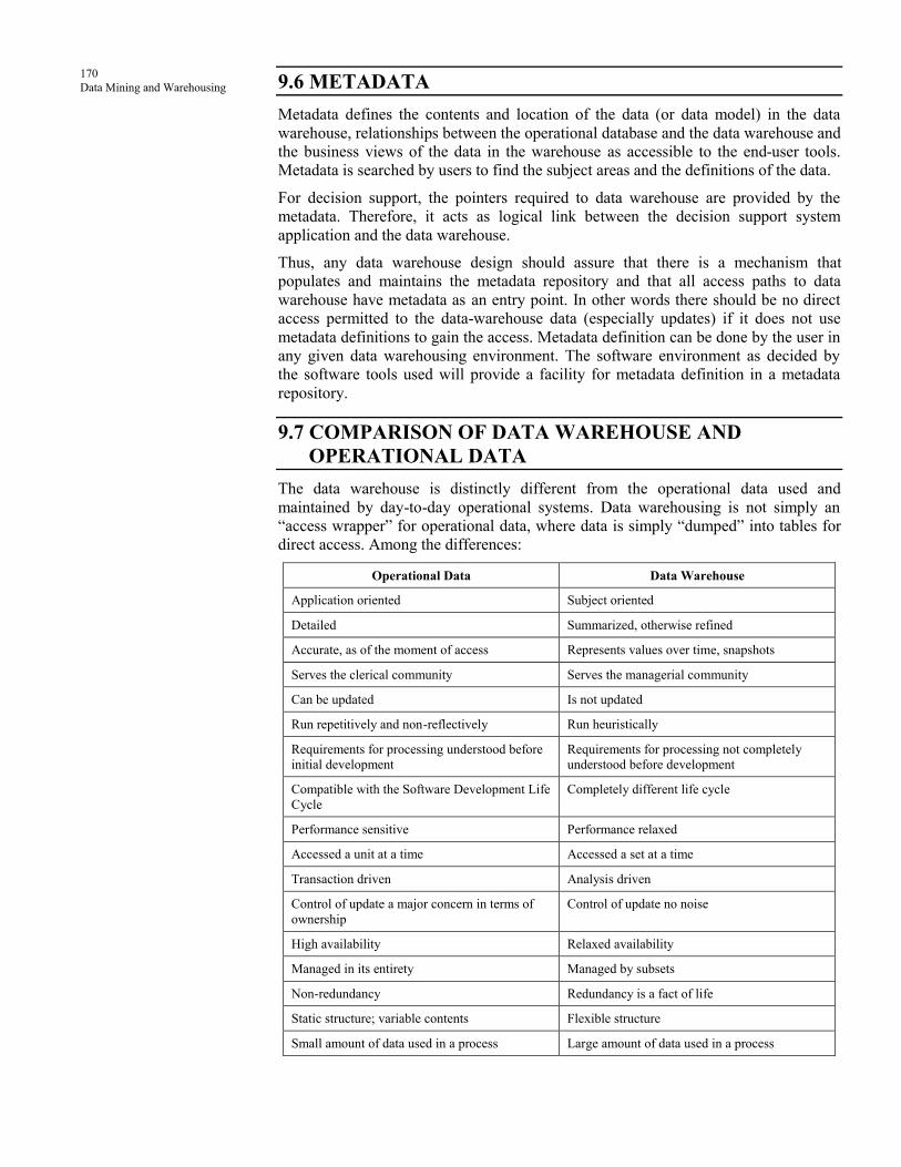
170


9.6 METADATA

Metadata defines the contents and location of the data (or data model) in the data

warehouse, relationships between the operational database and the data warehouse and

the business views of the data in the warehouse as accessible to the end-user tools.

Metadata is searched by users to find the subject areas and the definitions of the data.

For decision support, the pointers required to data warehouse are provided by the

metadata. Therefore, it acts as logical link between the decision support system

application and the data warehouse.

Thus, any data warehouse design should assure that there is a mechanism that

populates and maintains the metadata repository and that all access paths to data

warehouse have metadata as an entry point. In other words there should be no direct

access permitted to the data-warehouse data (especially updates) if it does not use

metadata definitions to gain the access. Metadata definition can be done by the user in

any given data warehousing environment. The software environment as decided by

the software tools used will provide a facility for metadata definition in a metadata

repository.

9.7 COMPARISON OF DATA WAREHOUSE AND

OPERATIONAL DATA

The data warehouse is distinctly different from the operational data used and

maintained by day-to-day operational systems. Data warehousing is not simply an

“access wrapper” for operational data, where data is simply “dumped” into tables for

direct access. Among the differences:

Operational Data Data Warehouse

Application oriented Subject oriented

Detailed Summarized, otherwise refined

Accurate, as of the moment of access Represents values over time, snapshots

Serves the clerical community Serves the managerial community

Can be updated Is not updated

Run repetitively and non-reflectively Run heuristically

Requirements for processing understood before

initial development

Requirements for processing not completely

understood before development

Compatible with the Software Development Life

Cycle

Completely different life cycle

Performance sensitive Performance relaxed

Accessed a unit at a time Accessed a set at a time

Transaction driven Analysis driven

Control of update a major concern in terms of

ownership

Control of update no noise

High availability Relaxed availability

Managed in its entirety Managed by subsets

Non-redundancy Redundancy is a fact of life

Static structure; variable contents Flexible structure

Small amount of data used in a process Large amount of data used in a process

171

Developing Data

Warehouse

9.8 DISTRIBUTION OF DATA

As the data warehouse grows in size, it becomes important to decide which data is to

be located where, in which server in the network, etc. Data distribution can be planned

so as to be based on subject area, location (or region) or time (e.g. monthly, yearly). In

other words, the data can be distributed location-wise, time-wise or subject-wise. The

distribution of data should be optimal for the data itself and also for querying

purposes. The performance of queries depends upon the location and distribution of

the data as the retrieval time is also dependent on the easy and fast accessibility.

9.9 TOOLS FOR DATA WAREHOUSING

For various stages or steps involved in the development of the data warehouse, a

number of tools are available from different vendors in the market. Some tools are

single vendor-based for several stages or quite often multiple vendor sources will be

required for different tools in different stages. These tools provide facilities for

defining the transformation and clean-up, data movement from operational data

sources into the warehouse, end-user querying, reporting and finally for data analysis

and data mining. Each tools takes a slightly different approach to data warehousing

and often maintains its own version of metadata repository. It is important that the

designer of the data warehouse may not sacrifice or dedicate the entire design process

so as to fit a specific tools. In the process, loss of semantics many happen if the tool is

weak. Therefore, it is better to go for a very comprehensive tool. It is also very

important to ensure that all the related tools are compatible with one another and also

with the overall design.

All the tools should also the compatible with the given data warehousing environment

and also with one another. This means that all the selected tools are compatible with

each other and there can be a common metadata repository. Alternatively, the tools

should be able to source the metadata from the warehouse data dictionary or from a

CASE tool used to design the database in the data warehouse. Another option is to use

metadata gateways that translate one tool’s metadata to another tool’s format.

If the above guidelines are not meticulously followed then the resulting data

warehouse environment will rapidly become unmanageable since every modification

to the warehouse data model may involve some significant and labour-intensive

changes to the metadata definitions for every tool in the environment. These changes

will also be required to be verified for consistency and integrity.

9.10 PERFORMANCE CONSIDERATIONS

Even though OLAP applications on a data warehouse are not calling for every

stringent, real-time responses as in the case of OLTP systems in a database, the

interactions of the user with data warehouse should be online and interactive with

good enough speed. Rapid query processing is desirable.

The actual performance levels may vary from application to application with different

requirements, as the case may be. The requirements of query response time, as defined

by a particular business application, are required to be met fully by the data warehouse

and its tools. However, it is not possible to predict in advance the performance levels

of a data warehouse. As the usage patterns of the data warehousing vary from

application and are unpredictable, the traditional database design and tuning

techniques do not always work in data warehouse environment.

It is essential therefore to understand and know the specific user requirements in terms

of the information and querying before the data warehouse is designed and

implemented. Query optimization also can be done if frequently asked queries are

well understood. For example, to answer aggregate level queries the warehouse can be

172


populated with specified denormalized view containing specific, summarized, derived

and aggregated data.

If made correctly available, many end-user requirements and many frequently asked

queries can be answered directly and efficiently so that the overall performance levels

can be maintained high.

9.11 CRUCIAL DECISION IN DESIGNING A DATA

WAREHOUSE

The job of designing and implementing a data warehouse is very challenging and

difficult one, even though at the same time, there is a lot of focus and importance

attached to it. The designer of a data warehouse may be asked by the top management:

“The all enterprise data and build a data warehouse such that the management can get

answers to all their questions”. This is a daunting task with responsibility being visible

and exciting. But how to get started? Where to start? Which data should be put first?

Where is that data available? Which queries should be answered? How would bring

down the scope of the project to something smaller and manageable, yet be scalable to

gradually upgrade to build a comprehensive data warehouse environment finally?

The recent trend is to build data marts before a real large data warehouse is built.

People want something smaller, so as to get manageable results before proceeding to a

real data warehouse.

Ralph Kimball identified a nine-step method as follows:

Step 1: Choose the subject matter (one at a time)

Step 2: Decide what the fact table represents

Step 3: Identify and conform the dimensions

Step 4: Choose the facts

Step 5: Store pre-calculations in the fact table

Step 6: Define the dimensions and tables

Step 7: Decide the duration of the database and periodicity of updation

Step 8: Track slowly the changing dimensions

Step 9: Decide the query priorities and the query modes.

All the above steps are required before the data warehouse is implemented. The final

step or step 10 is to implement a simple data warehouse or a data mart. The approach

should be ‘from simpler to complex’.

First, only a few data marts are identifies, designed and implemented. A data

warehouse then will emerge gradually.

Let us discuss the above mentioned steps in detail. Interaction with the users is

essential for obtaining answers to many of the above questions. The users to be

interviewed include top management, middle management, executives as also

operational users, in addition to salesforce and marketing teams. A clear picture

emerges from the entire project on data warehousing as to what are their problems and

how they can possibly be solved with the help of the data warehousing.

The priorities of the business issues can also be found. Similarly, interviewing the

DBAs in the organization will also give a clear picture as what are the data sources

with clean data, valid data and consistent data with assured flow for several years.

173

Developing Data

Warehouse

Check Your Progress


…………………………………..………………………………………….

…………………………………..………………………………………….

2. Define Data Content

…………………………………..………………………………………….

…………………………………..………………………………………….

9.12 LET US SUM UP

In this lesson, you learnt, the process of data warehouse development, what are the

strategies of organization behind the establishment of data warehouse. You understand

the data content and metadata consideration of data tools. You also learnt in this unit,

warehousing performance consideration, and crucial decision on designing a data

warehouse.


Discuss crucial decision in designing data warehouse.

9.14 KEYWORDS

Metadata: Metadata defines the contents and location of the data (or data model) in

the data warehouse, relationships between the operational database and the data

warehouse and the business views of the data in the warehouse as accessible to the

end-user tools.

Data warehouse: A data warehouse is a subject-oriented, integrated, time-variant, and

nonvolatile collection of data in support of management’s decision making process.

OLAP: Online analytical processing


1. What do you mean by Data contents?

2. Why and how to build a data warehouse architectural strategies?

3. Differentiate data warehouse and operational data.

4. What do you mean by distribution of data?


1. A data warehouse is a subject-oriented, integrated, time-variant, and non-

volatile collection of data in support of management’s decision making

process.

2. It is normally misunderstood that data warehouse contains lesser level of

detailed data when compared on an OLTP system which may be its

source. This is incorrect. The level of detail of data in the data warehouse

is normally the same as that of the source OLTP system; only it may be in

a different format. Typically, a data source contains detail level data. But

the data is cleaned and transferred to fit in the data warehouse model.

174






1993.












Edition, 2004.


Publications, 2004.




Edition, 2000.

175

Application of Data Warehousing

and Mining in Government LESSON

10 APPLICATION OF DATA WAREHOUSING AND MINING

IN GOVERNMENT

CONTENTS


10.1 Introduction

10.2 National Data Warehouses

10.2.1 Census Data

10.2.2 Prices of Essential Commodities

10.3 Other Areas for Data Warehousing and Data Mining

10.4 Let us Sum up


10.6 Keywords





The concept of national data warehouse

Basic knowledge of other areas for data warehousing and data mining

10.1 INTRODUCTION

Data warehousing and data mining are the important means of preparing the

government to face the challenges of the new millennium.

Data warehousing and data mining technologies have extensive potential applications

in the government—in various Central Government sectors such as Agriculture, Rural

Development, Health and Energy and also in State Government activities. These

technologies can and should therefore be implemented.

In this lesson, we shall examine their potential applications in the State and Central

Government.

10.2 NATIONAL DATA WAREHOUSES

A large number of national data warehouse can be identifies from the existing data

resources within the Central Government Ministries. Let us examine these potential

subject areas on which data warehouses may be developed at present and also in

future.

176


10.2.1 Census Data

The registrar General of Census Commissioner of India decennially compiles

information of all individuals, villages, population groups, etc. This information is

wide ranging households, of which a database of 5% sample is maintained for

analysis. A data warehouse can be built from this database upon which OLAP

techniques can be applied. Data mining also can be performed for analysis and

knowledge discovery.

A village-level database was originally developed by National Informatics Centre at

Hyderabad under General Information Services Terminal of National Informatics

Centre (GISTNIC) for the 1991 Census. This consists of two parts: primary census

abstract and village amenities. Subsequently, a data warehouse was also developed for

village amenities for Tamil Nadu. This enables multidimensional analysis of the

village level data in such sectors as Education, Health and Infrastructure. The fact data

pertains to the individual village data compiled under 1991 Census.

As the census compilation is performed once in ten years, the data is quasi-static and,

therefore, no refreshing of the warehouse needs to be done on a periodic basis. Only

the new data needs to be either appended to the data warehouse or alternatively a new

data warehouse can be built.

There exist many other subject areas (e.g. migration tables) within the census preview

which may be amenable and appropriate for data warehouse development, OLAP and

data mining applications on which work can be taken up in future.

10.2.2 Prices of Essential Commodities

The ministry of food and Civil Supplies, Government of India, compiles daily data for

about 300 observation centers in the entire country on the prices of essential

commodities such as rice, edible oils, etc. this data is compiled at the district level by

the respective State Government agencies and transmitted online to Delhi for

aggregation and storage. A data warehouse can be built for this data, and OLAP

Techniques can be applied for its analysis. A data mining and forecasting technique

can be applied for advance forecasting of the actual prices of these essential

commodities. The forecasting model can be strengthened for more accurate

forecasting by taking into account the external factors such as rainfall, growth rate of

population and inflation.

A limited exercise in this direction was already executed at a State level.

10.3 OTHER AREAS FOR DATA WAREHOUSING AND

DATA MINING

Other possible areas for data warehousing and data mining in Central Government

sectors are discussed in detail as under.

Agriculture

The Agriculture Census performed by the ministry of Agriculture, Government of

India, compiles a large number of agriculture parameters at the national level. District-

wise agriculture production, area and yield of crops is compiled; this can be built a

data warehouse for analysis, mining and forecasting. Statistics on consumption of

fertilizers also can be turned into a data mart.

Data on agriculture inputs such as seeds and fertilizers can also be effectively

analyzed in a date warehouse. Data form livestock census can be turned into a data

warehouse. Land-use pattern statistics can also be analyzed in a warehousing

environment. Other data such as watershed details and also agricultural credit data can

be effectively used for analysis by applying the technologies of OLAP and data

mining.

177


and Mining in Government

Thus there is substantial scope for application of data warehousing and data mining

techniques in Agriculture sector.

Rural Development

Data on individuals below poverty line (BPL survey) can be built into a data

warehouse. Drinking water census data can be effectively utilized by OLAP and data

mining technologies. Monitoring and analysis of progress made on implementation of

rural development programmers can also be made using OLAP and data mining

techniques.

Health

Community needs assessment data, immunization data, data from national

programmes on controlling blindness, leprosy, malaria can all be used for data

warehousing implementation, OLAP and data mining applications.

Planning

At the planning Commission, data warehouses can be built for state plan data on all

sectors: labour, energy, education, trade and industry, five year plan, etc.

Education

The sixth All India Educational Survey data has been converted into a data warehouse

(with about 3 GB of data). Various types of analytical queries and reports can be

answered.

Commerce and Trade

Data bank on trade can be analyzed and converted into a data warehouse. World price

monitoring system can be made to perform better by using data warehousing and data

mining technologies. Provisional estimates of import and export also be made more

accurate using forecasting techniques.

Other Sectors

In addition to the above mentioned important applications, there exist a number of

other potential application areas for data warehousing and data mining, as follows:

Tourism: Tourism arrival behaviour and preferences; tourism products data;

foreign exchange earning data; and Hotels, Travel and Transportation data.

Programme Implementation: Central projects data (for monitoring).

Revenue: Customs data, central excise data, and commercial taxes data (state

government).

Economic affairs: Budget and expenditure data; and annual economic survey.

Audit and accounts: Government accounts data.

All government departments or organizations are deeply involved in generating and

processing a large amount of data. Conventionally, the government departments have

largely been satisfied with developing single management information system (MIS),

or in limited cases, a few databases which were used online for limited reporting

purpose. Much of the analysis work was done manually by the Department of

Statistics in the Central Government or in any State Government. The techniques used

for analysis were conventional statistical techniques on largely batch-mode

processing. Prior to the advent of data warehousing and data mining technologies

nobody was aware of any better techniques for this activity. In fact, data warehousing

and data mining technologies could lead to the most significant advancements in the

government functioning, if properly applied and used in the government activities.

178


With their advent and prominence, there is a paradigm shift which may finally result

in improved governance and better planning by better utilization of data. Instead of

the officials wasting their time in processing data, they can rely on data warehousing

and data mining technologies for their day-to-day decision making and concentrate

more on the practical implementation of the decision so taken for better performance

of developmental activities.

Further, even though various departments in the government (State or Central) are

functionally interlinked, the data is presently generated, maintained and used

independently in each department. This leads to poor decision making and isolated

planning. Here in lies the importance of data warehousing technology. Different data

marts for separate departments, if built, can be integrated into one data warehouse for

the government. This is true for State Government and Central Government. Thus

data warehouses can be built at Central level, State level and also at District level.

Check Your Progress

What do you mean by rural development?

…………………………………..……………………………………………...

…………………………………..……………………………………………...

10.4 LET US SUM UP

In the government, the individual data marts required to be maintained by the

individual departments and a central data warehouse is required to be maintained by

the ministry concerned for the concerned sector. A generic inter-sectoral data

warehouse is required to be maintained by a central body. Similarity, at the State

level, a generic inter-departmental data warehouse can be built and maintained by a

nodal agency, and detailed data warehouses can also be built and maintained at the

district level by an appropriate agency. National Informatics Centre may possible play

the role of the nodal agency at Central, State and District levels for developing and

maintaining data warehouses in various sectors.


Discuss other areas of data warehouse and data mining.

10.6 KEYWORDS

Revenue: Customs data, central excise data, and commercial taxes data (state

government).

Economic affairs: Budget and expenditure data; and annual economic survey.


1. What do you mean by National Data Warehouse?

2. Explain the various areas of data warehousing and data mining.


Data on individuals below poverty line (BPL Survey) can be built into a data

warehouse. Drinking water census data can be effectively utilized by OLAP

and data mining technologies. Monitoring and analysis of progress made on

implementation of rural development programmes can also be made using

OLAP and data mining techniques.

179


and Mining in Government





1993.












Edition, 2004.


Publications, 2004.




Edition, 2000.

118


181

Model Question Paper MODEL QUESTION PAPER

MCA

Third Year

Sub: Data Mining and Warehousing

Time: 3 hours Total Marks: 100

Direction: There are total eight questions, each carrying 20 marks. You have to

attempt any five questions.

1. Why data mining is crucial to the success of a business?

2. Briefly discuss the issues of data mining.

3. What do you mean by data cleaning?

4. Write short notes on:

(a) Model based clustering

(b) K-medoid algorithm

(c) Market basket analysis

(d) Data warehouse DBMS selection

5. How a data warehouse is different from data base? Explain with the help of

suitable example.

6. What is the process of designing a data warehouse?

7. What do you mean by Data contents?

8. Explain the various areas of data warehousing and data mining.

data mining and warehousing - ace

Documents