data mining: concepts and techniques€¦ · · 2012-01-06data mining: concepts and techniques...
TRANSCRIPT

Data Mining: Concepts andTechniques
3rd Edition
Solution Manual
Jiawei Han, Micheline Kamber, Jian Pei
The University of Illinois at Urbana-Champaign
Simon Fraser University
Version January 2, 2012
c⃝Morgan Kaufmann, 2011
For Instructors’ references only.
Do not copy! Do not distribute!

ii

Preface
For a rapidly evolving field like data mining, it is difficult to compose “typical” exercises and even moredifficult to work out “standard” answers. Some of the exercises in Data Mining: Concepts and Techniquesare themselves good research topics that may lead to future Master or Ph.D. theses. Therefore, our solutionmanual is intended to be used as a guide in answering the exercises of the textbook. You are welcome toenrich this manual by suggesting additional interesting exercises and/or providing more thorough, or betteralternative solutions.
While we have done our best to ensure the correctness of the solutions, it is possible that some typos orerrors may exist. If you should notice any, please feel free to point them out by sending your suggestions [email protected]. We appreciate your suggestions.
To assist the teachers of this book to work out additional homework or exam questions, we have addedone additional section “Supplementary Exercises” to each chapter of this manual. This section includesadditional exercise questions and their suggested answers and thus may substantially enrich the value of thissolution manual. Additional questions and answers will be incrementally added to this section, extractedfrom the assignments and exam questions of our own teaching. To this extent, our solution manual will beincrementally enriched and subsequently released in the future months and years.
Notes to the current release of the solution manual.
Due to the limited time, this release of the solution manual is a preliminary version. Many of the newlyadded exercises in the third edition have not provided the solutions yet. We apologize for the inconvenience.We will incrementally add answers to those questions in the next several months and release the new versionsof updated solution manual in the subsequent months.
Acknowledgements
For each edition of this book, the solutions to the exercises were worked out by different groups of teachassistants and students. We sincerely express our thanks to all the teaching assistants and participatingstudents who have worked with us to make and improve the solutions to the questions. In particular, for thefirst edition of the book, we would like to thanks Denis M. C. Chai, Meloney H.-Y. Chang, James W. Herdy,Jason W. Ma, Jiuhong Xu, Chunyan Yu, and Ying Zhou who took the class of CMPT-459: Data Mining andData Warehousing at Simon Fraser University in the Fall semester of 2000 and contributed substantially tothe solution manual of the first edition of this book. For those questions that also appear in the first edition,the answers in this current solution manual are largely based on those worked out in the preparation of thefirst edition.
For the solution manual of the second edition of the book, we would like to thank Ph.D. students andteaching assistants, Deng Cai and Hector Gonzalez, for the course CS412: Introduction to Data Mining andData Warehousing, offered in the Fall semester of 2005 in the Department of Computer Science at theUniversity of Illinois at Urbana-Champaign. They have helped prepare and compile the answers for the newexercises of the first seven chapters in our second edition. Moreover, our thanks go to several students fromthe CS412 class in the Fall semester of 2005 and the CS512: Data Mining: Principles and Algorithms classes
iii

iv
in the Spring semester of 2006. Their answers to the class assignments have contributed to the advancementof this solution manual.
For the solution manual of the third edition of the book, we would like to thank Ph.D. students, Jialu Liu,Brandon Norick and Jingjing Wang, in the course CS412: Introduction to Data Mining and Data Warehousing,offered in the Fall semester of 2011 in the Department of Computer Science at the University of Illinoisat Urbana-Champaign. They have helped checked the answers of the previous editions and did manymodifications, and also prepared and compiled the answers for the new exercises in this edition. Moreover,our thanks go to teaching assistants, Xiao Yu, Lu An Tang, Xin Jin and Peixiang Zhao, from the CS412 classand the CS512: Data Mining: Principles and Algorithms classes in the years of 2008–2011. Their answersto the class assignments have contributed to the advancement of this solution manual.

Contents
1 Introduction 3
1.1 Exercises . . . . . . . . . . . . . . . . . . . . . . . . . . . . . . . . . . . . . . . . . . . . . . . 3
1.2 Supplementary Exercises . . . . . . . . . . . . . . . . . . . . . . . . . . . . . . . . . . . . . . . 7
2 Getting to Know Your Data 11
2.1 Exercises . . . . . . . . . . . . . . . . . . . . . . . . . . . . . . . . . . . . . . . . . . . . . . . 11
2.2 Supplementary Exercises . . . . . . . . . . . . . . . . . . . . . . . . . . . . . . . . . . . . . . . 18
3 Data Preprocessing 19
3.1 Exercises . . . . . . . . . . . . . . . . . . . . . . . . . . . . . . . . . . . . . . . . . . . . . . . 19
3.2 Supplementary Exercises . . . . . . . . . . . . . . . . . . . . . . . . . . . . . . . . . . . . . . . 31
4 Data Warehousing and Online Analytical Processing 33
4.1 Exercises . . . . . . . . . . . . . . . . . . . . . . . . . . . . . . . . . . . . . . . . . . . . . . . 33
4.2 Supplementary Exercises . . . . . . . . . . . . . . . . . . . . . . . . . . . . . . . . . . . . . . . 47
5 Data Cube Technology 49
5.1 Exercises . . . . . . . . . . . . . . . . . . . . . . . . . . . . . . . . . . . . . . . . . . . . . . . 49
5.2 Supplementary Exercises . . . . . . . . . . . . . . . . . . . . . . . . . . . . . . . . . . . . . . . 67
6 Mining Frequent Patterns, Associations, and Correlations: Basic Concepts and Methods 69
6.1 Exercises . . . . . . . . . . . . . . . . . . . . . . . . . . . . . . . . . . . . . . . . . . . . . . . 69
6.2 Supplementary Exercises . . . . . . . . . . . . . . . . . . . . . . . . . . . . . . . . . . . . . . . 78
7 Advanced Pattern Mining 79
7.1 Exercises . . . . . . . . . . . . . . . . . . . . . . . . . . . . . . . . . . . . . . . . . . . . . . . 79
7.2 Supplementary Exercises . . . . . . . . . . . . . . . . . . . . . . . . . . . . . . . . . . . . . . . 88
8 Classification: Basic Concepts 91
8.1 Exercises . . . . . . . . . . . . . . . . . . . . . . . . . . . . . . . . . . . . . . . . . . . . . . . 91
8.2 Supplementary Exercises . . . . . . . . . . . . . . . . . . . . . . . . . . . . . . . . . . . . . . . 99
9 Classification: Advanced Methods 101
9.1 Exercises . . . . . . . . . . . . . . . . . . . . . . . . . . . . . . . . . . . . . . . . . . . . . . . 101
9.2 Supplementary Exercises . . . . . . . . . . . . . . . . . . . . . . . . . . . . . . . . . . . . . . . 105
10 Cluster Analysis: Basic Concepts and Methods 107
10.1 Exercises . . . . . . . . . . . . . . . . . . . . . . . . . . . . . . . . . . . . . . . . . . . . . . . 107
10.2 Supplementary Exercises . . . . . . . . . . . . . . . . . . . . . . . . . . . . . . . . . . . . . . . 115
v

CONTENTS 1
11 Advanced Cluster Analysis 12311.1 Exercises . . . . . . . . . . . . . . . . . . . . . . . . . . . . . . . . . . . . . . . . . . . . . . . 123
12 Outlier Detection 12712.1 Exercises . . . . . . . . . . . . . . . . . . . . . . . . . . . . . . . . . . . . . . . . . . . . . . . 127
13 Trends and Research Frontiers in Data Mining 13113.1 Exercises . . . . . . . . . . . . . . . . . . . . . . . . . . . . . . . . . . . . . . . . . . . . . . . 13113.2 Supplementary Exercises . . . . . . . . . . . . . . . . . . . . . . . . . . . . . . . . . . . . . . . 139

2 CONTENTS

Chapter 1
Introduction
1.1 Exercises
1. What is data mining? In your answer, address the following:
(a) Is it another hype?
(b) Is it a simple transformation or application of technology developed from databases, statistics,machine learning, and pattern recognition?
(c) We have presented a view that data mining is the result of the evolution of database technology.Do you think that data mining is also the result of the evolution of machine learning research?Can you present such views based on the historical progress of this discipline? Do the same forthe fields of statistics and pattern recognition.
(d) Describe the steps involved in data mining when viewed as a process of knowledge discovery.
Answer:
Data mining refers to the process or method that extracts or “mines” interesting knowledge orpatterns from large amounts of data.
(a) Is it another hype?
Data mining is not another hype. Instead, the need for data mining has arisen due to the wideavailability of huge amounts of data and the imminent need for turning such data into usefulinformation and knowledge. Thus, data mining can be viewed as the result of the natural evolutionof information technology.
(b) Is it a simple transformation of technology developed from databases, statistics, and machinelearning?
No. Data mining is more than a simple transformation of technology developed from databases,statistics, and machine learning. Instead, data mining involves an integration, rather than asimple transformation, of techniques from multiple disciplines such as database technology, statis-tics, machine learning, high-performance computing, pattern recognition, neural networks, datavisualization, information retrieval, image and signal processing, and spatial data analysis.
(c) Explain how the evolution of database technology led to data mining.
Database technology began with the development of data collection and database creation mech-anisms that led to the development of effective mechanisms for data management including datastorage and retrieval, and query and transaction processing. The large number of database sys-tems offering query and transaction processing eventually and naturally led to the need for dataanalysis and understanding. Hence, data mining began its development out of this necessity.
3

4 CHAPTER 1. INTRODUCTION
(d) Describe the steps involved in data mining when viewed as a process of knowledge discovery.
The steps involved in data mining when viewed as a process of knowledge discovery are as follows:
• Data cleaning, a process that removes or transforms noise and inconsistent data
• Data integration, where multiple data sources may be combined
• Data selection, where data relevant to the analysis task are retrieved from the database
• Data transformation, where data are transformed or consolidated into forms appropriatefor mining
• Data mining, an essential process where intelligent and efficient methods are applied inorder to extract patterns
• Pattern evaluation, a process that identifies the truly interesting patterns representingknowledge based on some interestingness measures
• Knowledge presentation, where visualization and knowledge representation techniques areused to present the mined knowledge to the user
2. How is a data warehouse different from a database? How are they similar?
Answer:
Differences between a data warehouse and a database: A data warehouse is a repository of informa-tion collected from multiple sources, over a history of time, stored under a unified schema, and usedfor data analysis and decision support; whereas a database, is a collection of interrelated data thatrepresents the current status of the stored data. There could be multiple heterogeneous databaseswhere the schema of one database may not agree with the schema of another. A database systemsupports ad-hoc query and on-line transaction processing. For more details, please refer to the section“Differences between operational database systems and data warehouses.”
Similarities between a data warehouse and a database: Both are repositories of information, storinghuge amounts of persistent data.
3. Define each of the following data mining functionalities: characterization, discrimination, associationand correlation analysis, classification, regression, clustering, and outlier analysis. Give examples ofeach data mining functionality, using a real-life database that you are familiar with.
Answer:
Characterization is a summarization of the general characteristics or features of a target class ofdata. For example, the characteristics of students can be produced, generating a profile of all theUniversity first year computing science students, which may include such information as a high GPAand large number of courses taken.
Discrimination is a comparison of the general features of target class data objects with the generalfeatures of objects from one or a set of contrasting classes. For example, the general features of studentswith high GPA’s may be compared with the general features of students with low GPA’s. The resultingdescription could be a general comparative profile of the students such as 75% of the students withhigh GPA’s are fourth-year computing science students while 65% of the students with low GPA’s arenot.
Association is the discovery of association rules showing attribute-value conditions that occur fre-quently together in a given set of data. For example, a data mining system may find association ruleslike
major(X, “computing science””)⇒ owns(X, “personal computer”)
[support = 12%, confidence = 98%]

1.1. EXERCISES 5
where X is a variable representing a student. The rule indicates that of the students under study,12% (support) major in computing science and own a personal computer. There is a 98% probability(confidence, or certainty) that a student in this group owns a personal computer. Typically, associa-tion rules are discarded as uninteresting if they do not satisfy both a minimum support thresholdand a minimum confidence threshold. Additional analysis can be performed to uncover interestingstatistical correlations between associated attribute-value pairs.
Classification is the process of finding a model (or function) that describes and distinguishes dataclasses or concepts, for the purpose of being able to use the model to predict the class of objects whoseclass label is unknown. It predicts categorical (discrete, unordered) labels.
Regression, unlike classification, is a process to model continuous-valued functions. It is used topredict missing or unavailable numerical data values rather than (discrete) class labels.
Clustering analyzes data objects without consulting a known class label. The objects are clusteredor grouped based on the principle of maximizing the intraclass similarity and minimizing the interclasssimilarity. Each cluster that is formed can be viewed as a class of objects. Clustering can also facilitatetaxonomy formation, that is, the organization of observations into a hierarchy of classes that groupsimilar events together.
Outlier analysis is the analysis of outliers, which are objects that do not comply with the generalbehavior or model of the data. Examples include fraud detection based on a large dataset of creditcard transactions.
4. Present an example where data mining is crucial to the success of a business. What data miningfunctionalities does this business need (e.g., think of the kinds of patterns that could be mined)? Cansuch patterns be generated alternatively by data query processing or simple statistical analysis?
Answer:
A department store, for example, can use data mining to assist with its target marketing mail campaign.Using data mining functions such as association, the store can use the mined strong association rules todetermine which products bought by one group of customers are likely to lead to the buying of certainother products. With this information, the store can then mail marketing materials only to those kindsof customers who exhibit a high likelihood of purchasing additional products. Data query processingis used for data or information retrieval and does not have the means for finding association rules.Similarly, simple statistical analysis cannot handle large amounts of data such as those of customerrecords in a department store.
5. What is the difference between discrimination and classification? Between characterization and clus-tering? Between classification and regression? For each of these pairs of tasks, how are they similar?
Answer:
Discrimination differs from classification in that the former refers to a comparison of the generalfeatures of target class data objects with the general features of objects from one or a set of contrastingclasses, while the latter is the process of finding a set of models (or functions) that describe anddistinguish data classes or concepts for the purpose of being able to use the model to predict the classof objects whose class label is unknown. Discrimination and classification are similar in that they bothdeal with the analysis of class data objects.
Characterization differs from clustering in that the former refers to a summarization of the generalcharacteristics or features of a target class of data while the latter deals with the analysis of dataobjects without consulting a known class label. This pair of tasks is similar in that they both dealwith grouping together objects or data that are related or have high similarity in comparison to oneanother.

6 CHAPTER 1. INTRODUCTION
Classification differs from regression in that the former predicts categorical (discrete, unordered)labels while the latter predicts missing or unavailable, and often numerical, data values. This pair oftasks is similar in that they both are tools for prediction.
6. Based on your observation, describe another possible kind of knowledge that needs to be discovered bydata mining methods but has not been listed in this chapter. Does it require a mining methodologythat is quite different from those outlined in this chapter?
Answer:
There is no standard answer for this question and one can judge the quality of an answer based on thefreshness and quality of the proposal. For example, one may propose partial periodicity as a new kindof knowledge, where a pattern is partial periodic if only some offsets of a certain time period in a timeseries demonstrate some repeating behavior.
7. Outliers are often discarded as noise. However, one person’s garbage could be another’s treasure. Forexample, exceptions in credit card transactions can help us detect the fraudulent use of credit cards.Using fraudulence detection as an example, propose two methods that can be used to detect outliersand discuss which one is more reliable.
Answer:
There are many outlier detection methods. More details can be found in Chapter 12. Here we proposetwo methods for fraudulence detection:
a) Statistical methods (also known as model-based methods): Assume that the normal trans-action data follow some statistical (stochastic) model, then data not following the model areoutliers.
b) Clustering-based methods: Assume that the normal data objects belong to large and denseclusters, whereas outliers belong to small or sparse clusters, or do not belong to any clusters.
It is hard to say which one is more reliable. The effectiveness of statistical methods highly dependson whether the assumptions made for the statistical model hold true for the given data. And theeffectiveness of clustering methods highly depends on which clustering method we choose.
8. Describe three challenges to data mining regarding data mining methodology and user interactionissues.
Answer:
Challenges to data mining regarding data mining methodology and user interaction issues include thefollowing: mining different kinds of knowledge in databases, interactive mining of knowledge at multiplelevels of abstraction, incorporation of background knowledge, data mining query languages and ad hocdata mining, presentation and visualization of data mining results, handling noisy or incomplete data,and pattern evaluation. Below are the descriptions of the first three challenges mentioned:
Mining different kinds of knowledge in databases: Different users are interested in differentkinds of knowledge and will require a wide range of data analysis and knowledge discovery tasks suchas data characterization, discrimination, association, classification, clustering, trend and deviationanalysis, and similarity analysis. Each of these tasks will use the same database in different ways andwill require different data mining techniques.
Interactive mining of knowledge at multiple levels of abstraction: Interactive mining, withthe use of OLAP operations on a data cube, allows users to focus the search for patterns, providingand refining data mining requests based on returned results. The user can then interactively view thedata and discover patterns at multiple granularities and from different angles.
Incorporation of background knowledge: Background knowledge, or information regarding thedomain under study such as integrity constraints and deduction rules, may be used to guide the

1.2. SUPPLEMENTARY EXERCISES 7
discovery process and allow discovered patterns to be expressed in concise terms and at different levelsof abstraction. This helps to focus and speed up a data mining process or judge the interestingness ofdiscovered patterns.
9. What are the major challenges of mining a huge amount of data (such as billions of tuples) in comparisonwith mining a small amount of data (such as a few hundred tuple data set)?
Answer:
One challenge to data mining regarding performance issues is the efficiency and scalability of datamining algorithms. Data mining algorithms must be efficient and scalable in order to effectively extractinformation from large amounts of data in databases within predictable and acceptable running times.Another challenge is the parallel, distributed, and incremental processing of data mining algorithms.The need for parallel and distributed data mining algorithms has been brought about by the huge size ofmany databases, the wide distribution of data, and the computational complexity of some data miningmethods. Due to the high cost of some data mining processes, incremental data mining algorithmsincorporate database updates without the need to mine the entire data again from scratch.
10. Outline the major research challenges of data mining in one specific application domain, such asstream/sensor data analysis, spatiotemporal data analysis, or bioinformatics.
Answer:
Let’s take spatiotemporal data analysis for example. With the ever increasing amount of availabledata from sensor networks, web-based map services, location sensing devices etc., the rate at whichsuch kind of data are being generated far exceeds our ability to extract useful knowledge from them tofacilitate decision making and to better understand the changing environment. It is a great challengehow to utilize existing data mining techniques and create novel techniques as well to effectively exploitthe rich spatiotemporal relationships/patterns embedded in the datasets because both the temporaland spatial dimensions could add substantial complexity to data mining tasks. First, the spatial andtemporal relationships are information bearing and therefore need to be considered in data mining.Some spatial and temporal relationships are implicitly defined, and must be extracted from the data.Such extraction introduces some degree of fuzziness and/or uncertainty that may have an impact on theresults of the data mining process. Second, working at the level of stored data is often undesirable, andthus complex transformations are required to describe the units of analysis at higher conceptual levels.Third, interesting patterns are more likely to be discovered at the lowest resolution/granularity level,but large support is more likely to exist at higher levels. Finally, how to express domain independentknowledge and how to integrate spatiotemporal reasoning mechanisms in data mining systems are stillopen problems [1].
[1] J. Han and J. Gao, Research Challenges for Data Mining in Science and Engineering, in H. Kargupta,et al., (eds.), Next Generation of Data Mining, Chapman & Hall, 2009.
1.2 Supplementary Exercises
1. Suppose your task as a software engineer at Big-University is to design a data mining system toexamine their university course database, which contains the following information: the name, address,and status (e.g., undergraduate or graduate) of each student, the courses taken, and their cumulativegrade point average (GPA).
Describe the architecture you would choose. What is the purpose of each component of this architec-ture?
Answer:

8 CHAPTER 1. INTRODUCTION
A data mining architecture that can be used for this application would consist of the following majorcomponents:
• A database, data warehouse, or other information repository, which consists of the setof databases, data warehouses, spreadsheets, or other kinds of information repositories containingthe student and course information.
• A database or data warehouse server which fetches the relevant data based on users’ datamining requests.
• A knowledge base that contains the domain knowledge used to guide the search or to evaluatethe interestingness of resulting patterns. For example, the knowledge base may contain metadatawhich describes data from multiple heterogeneous sources.
• A data mining engine, which consists of a set of functional modules for tasks such as classifi-cation, association, classification, cluster analysis, and evolution and deviation analysis.
• A pattern evaluation module that works in tandem with the data mining modules by employ-ing interestingness measures to help focus the search towards interestingness patterns.
• A graphical user interface that allows the user an interactive approach to the data miningsystem.
2. Briefly describe the following advanced database systems and applications: object-relational databases,spatial databases, text databases, multimedia databases, the World Wide Web.
Answer:
An objected-oriented database is designed based on the object-oriented programming paradigmwhere data are a large number of objects organized into classes and class hierarchies. Each entity inthe database is considered as an object. The object contains a set of variables that describe the object,a set of messages that the object can use to communicate with other objects or with the rest of thedatabase system, and a set of methods where each method holds the code to implement a message.
A spatial database contains spatial-related data, which may be represented in the form of rasteror vector data. Raster data consists of n-dimensional bit maps or pixel maps, and vector data arerepresented by lines, points, polygons or other kinds of processed primitives, Some examples of spatialdatabases include geographical (map) databases, VLSI chip designs, and medical and satellite imagesdatabases.
A text database is a database that contains text documents or other word descriptions in the form oflong sentences or paragraphs, such as product specifications, error or bug reports, warning messages,summary reports, notes, or other documents.
A multimedia database stores images, audio, and video data, and is used in applications such aspicture content-based retrieval, voice-mail systems, video-on-demand systems, the World Wide Web,and speech-based user interfaces.
The World-Wide Web provides rich, world-wide, on-line information services, where data objectsare linked together to facilitate interactive access. Some examples of distributed information servicesassociated with the World-Wide Web include America Online, Yahoo!, AltaVista, and Prodigy.
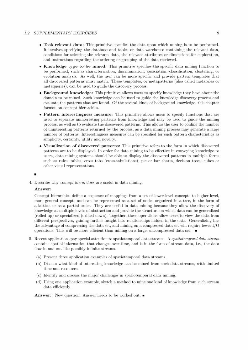
3. List and describe the five primitives for specifying a data mining task.
Answer:
The five primitives for specifying a data-mining task are:
1.2. SUPPLEMENTARY EXERCISES 9
• Task-relevant data: This primitive specifies the data upon which mining is to be performed.It involves specifying the database and tables or data warehouse containing the relevant data,conditions for selecting the relevant data, the relevant attributes or dimensions for exploration,and instructions regarding the ordering or grouping of the data retrieved.
• Knowledge type to be mined: This primitive specifies the specific data mining function tobe performed, such as characterization, discrimination, association, classification, clustering, orevolution analysis. As well, the user can be more specific and provide pattern templates thatall discovered patterns must match. These templates, or metapatterns (also called metarules ormetaqueries), can be used to guide the discovery process.
• Background knowledge: This primitive allows users to specify knowledge they have about thedomain to be mined. Such knowledge can be used to guide the knowledge discovery process andevaluate the patterns that are found. Of the several kinds of background knowledge, this chapterfocuses on concept hierarchies.
• Pattern interestingness measure: This primitive allows users to specify functions that areused to separate uninteresting patterns from knowledge and may be used to guide the miningprocess, as well as to evaluate the discovered patterns. This allows the user to confine the numberof uninteresting patterns returned by the process, as a data mining process may generate a largenumber of patterns. Interestingness measures can be specified for such pattern characteristics assimplicity, certainty, utility and novelty.
• Visualization of discovered patterns: This primitive refers to the form in which discoveredpatterns are to be displayed. In order for data mining to be effective in conveying knowledge tousers, data mining systems should be able to display the discovered patterns in multiple formssuch as rules, tables, cross tabs (cross-tabulations), pie or bar charts, decision trees, cubes orother visual representations.
4. Describe why concept hierarchies are useful in data mining.
Answer:
Concept hierarchies define a sequence of mappings from a set of lower-level concepts to higher-level,more general concepts and can be represented as a set of nodes organized in a tree, in the form ofa lattice, or as a partial order. They are useful in data mining because they allow the discovery ofknowledge at multiple levels of abstraction and provide the structure on which data can be generalized(rolled-up) or specialized (drilled-down). Together, these operations allow users to view the data fromdifferent perspectives, gaining further insight into relationships hidden in the data. Generalizing hasthe advantage of compressing the data set, and mining on a compressed data set will require fewer I/Ooperations. This will be more efficient than mining on a large, uncompressed data set.
5. Recent applications pay special attention to spatiotemporal data streams. A spatiotemporal data streamcontains spatial information that changes over time, and is in the form of stream data, i.e., the dataflow in-and-out like possibly infinite streams.
(a) Present three application examples of spatiotemporal data streams.
(b) Discuss what kind of interesting knowledge can be mined from such data streams, with limitedtime and resources.
(c) Identify and discuss the major challenges in spatiotemporal data mining.
(d) Using one application example, sketch a method to mine one kind of knowledge from such streamdata efficiently.
Answer: New question. Answer needs to be worked out.

10 CHAPTER 1. INTRODUCTION
6. Describe the differences between the following approaches for the integration of a data mining systemwith a database or data warehouse system: no coupling, loose coupling, semitight coupling, and tightcoupling. State which approach you think is the most popular, and why.
Answer: The differences between the following architectures for the integration of a data miningsystem with a database or data warehouse system are as follows.
• No coupling: The data mining system uses sources such as flat files to obtain the initial dataset to be mined since no database system or data warehouse system functions are implementedas part of the process. Thus, this architecture represents a poor design choice.
• Loose coupling: The data mining system is not integrated with the database or data warehousesystem beyond their use as the source of the initial data set to be mined, and possible use instorage of the results. Thus, this architecture can take advantage of the flexibility, efficiency andfeatures such as indexing that the database and data warehousing systems may provide. However,it is difficult for loose coupling to achieve high scalability and good performance with large datasets as many such systems are memory-based.
• Semitight coupling: Some of the data mining primitives such as aggregation, sorting or pre-computation of statistical functions are efficiently implemented in the database or data warehousesystem, for use by the data mining system during mining-query processing. Also, some frequentlyused intermediate mining results can be precomputed and stored in the database or data ware-house system, thereby enhancing the performance of the data mining system.
• Tight coupling: The database or data warehouse system is fully integrated as part of the datamining system and thereby provides optimized data mining query processing. Thus, the datamining subsystem is treated as one functional component of an information system. This is ahighly desirable architecture as it facilitates efficient implementations of data mining functions,high system performance, and an integrated information processing environment.
From the descriptions of the architectures provided above, it can be seen that tight coupling is the bestalternative without respect to technical or implementation issues. However, as much of the technicalinfrastructure needed in a tightly coupled system is still evolving, implementation of such a system isnon-trivial. Therefore, the most popular architecture is currently semitight coupling as it provides acompromise between loose and tight coupling.

Chapter 2
Getting to Know Your Data
2.1 Exercises
1. Give three additional commonly used statistical measures (i.e., not illustrated in this chapter) for thecharacterization of data dispersion, and discuss how they can be computed efficiently in large databases.
Answer:
Data dispersion, also known as variance analysis, is the degree to which numeric data tend to spreadand can be characterized by such statistical measures as mean deviation, measures of skewness andthe coefficient of variation.
The mean deviation is defined as the arithmetic mean of the absolute deviations from the meansand is calculated as:
mean deviation =
∑ni=1 |x− x|
n(2.1)
where, x is the arithmetic mean of the values and n is the total number of values. This value will begreater for distributions with a larger spread.
A common measure of skewness is:
x−mode
s(2.2)
which indicates how far (in standard deviations, s) the mean (x) is from the mode and whether it isgreater or less than the mode.
The coefficient of variation is the standard deviation expressed as a percentage of the arithmeticmean and is calculated as:
coefficient of variation =s
x× 100 (2.3)
The variability in groups of observations with widely differing means can be compared using thismeasure.
Note that all of the input values used to calculate these three statistical measures are algebraic measures(Chapter 4). Thus, the value for the entire database can be efficiently calculated by partitioning thedatabase, computing the values for each of the separate partitions, and then merging theses values intoan algebraic equation that can be used to calculate the value for the entire database.
11

12 CHAPTER 2. GETTING TO KNOW YOUR DATA
The measures of dispersion described here were obtained from: Statistical Methods in Research andProduction, fourth ed., Edited by Owen L. Davies and Peter L. Goldsmith, Hafner Publishing Company,NY:NY, 1972.
2. Suppose that the data for analysis includes the attribute age. The age values for the data tuples are(in increasing order) 13, 15, 16, 16, 19, 20, 20, 21, 22, 22, 25, 25, 25, 25, 30, 33, 33, 35, 35, 35, 35, 36,40, 45, 46, 52, 70.
(a) What is the mean of the data? What is the median?
(b) What is the mode of the data? Comment on the data’s modality (i.e., bimodal, trimodal, etc.).
(c) What is the midrange of the data?
(d) Can you find (roughly) the first quartile (Q1) and the third quartile (Q3) of the data?
(e) Give the five-number summary of the data.
(f) Show a boxplot of the data.
(g) How is a quantile-quantile plot different from a quantile plot?
Answer:
(a) What is the mean of the data? What is the median?
The (arithmetic) mean of the data is: x = 1n
∑ni=1 xi = 809/27 = 30. The median (middle value
of the ordered set, as the number of values in the set is odd) of the data is: 25.
(b) What is the mode of the data? Comment on the data’s modality (i.e., bimodal, trimodal, etc.).
This data set has two values that occur with the same highest frequency and is, therefore, bimodal.The modes (values occurring with the greatest frequency) of the data are 25 and 35.
(c) What is the midrange of the data?
The midrange (average of the largest and smallest values in the data set) of the data is: (70 +13)/2 = 41.5
(d) Can you find (roughly) the first quartile (Q1) and the third quartile (Q3) of the data?
The first quartile (corresponding to the 25th percentile) of the data is: 20. The third quartile(corresponding to the 75th percentile) of the data is: 35.
(e) Give the five-number summary of the data.
The five number summary of a distribution consists of the minimum value, first quartile, medianvalue, third quartile, and maximum value. It provides a good summary of the shape of thedistribution and for this data is: 13, 20, 25, 35, 70.
(f) Show a boxplot of the data.
See Figure 2.1.
(g) How is a quantile-quantile plot different from a quantile plot?
A quantile plot is a graphical method used to show the approximate percentage of values belowor equal to the independent variable in a univariate distribution. Thus, it displays quantileinformation for all the data, where the values measured for the independent variable are plottedagainst their corresponding quantile.
A quantile-quantile plot however, graphs the quantiles of one univariate distribution against thecorresponding quantiles of another univariate distribution. Both axes display the range of valuesmeasured for their corresponding distribution, and points are plotted that correspond to thequantile values of the two distributions. A line (y = x) can be added to the graph along withpoints representing where the first, second and third quantiles lie, in order to increase the graph’sinformational value. Points that lie above such a line indicate a correspondingly higher value forthe distribution plotted on the y-axis, than for the distribution plotted on the x-axis at the samequantile. The opposite effect is true for points lying below this line.

2.1. EXERCISES 13
age
2030
4050
6070
Val
ues
Figure 2.1: A boxplot of the data in Exercise 2.2.
3. Suppose that the values for a given set of data are grouped into intervals. The intervals and corre-sponding frequencies are as follows.
age frequency1–5 2006–15 45016–20 30021–50 150051–80 70081–110 44
Compute an approximate median value for the data.
Answer:
L1 = 20, n= 3194, (∑
f )l = 950, freq median = 1500, width = 30, median = 30.94 years.
4. Suppose a hospital tested the age and body fat data for 18 randomly selected adults with the followingresult
age 23 23 27 27 39 41 47 49 50%fat 9.5 26.5 7.8 17.8 31.4 25.9 27.4 27.2 31.2
age 52 54 54 56 57 58 58 60 61%fat 34.6 42.5 28.8 33.4 30.2 34.1 32.9 41.2 35.7
(a) Calculate the mean, median and standard deviation of age and %fat.
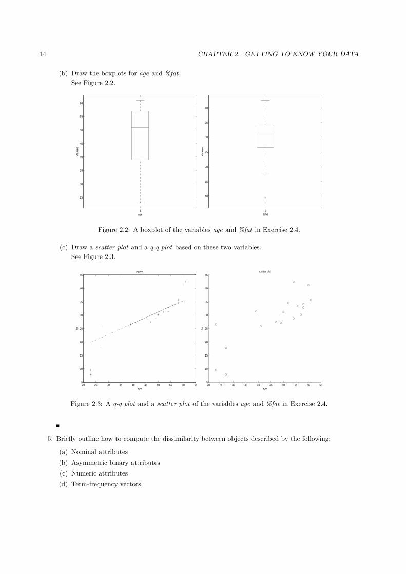
(b) Draw the boxplots for age and %fat.
(c) Draw a scatter plot and a q-q plot based on these two variables.
Answer:
(a) Calculate the mean, median and standard deviation of age and %fat.
For the variable age the mean is 46.44, the median is 51, and the standard deviation is 12.85. Forthe variable %fat the mean is 28.78, the median is 30.7, and the standard deviation is 8.99.
14 CHAPTER 2. GETTING TO KNOW YOUR DATA
(b) Draw the boxplots for age and %fat.
See Figure 2.2.
1
25
30
35
40
45
50
55
60
Valu
es
age1
10
15
20
25
30
35
40
Valu
es
%fat
Figure 2.2: A boxplot of the variables age and %fat in Exercise 2.4.
(c) Draw a scatter plot and a q-q plot based on these two variables.
See Figure 2.3.
20 25 30 35 40 45 50 55 60 655
10
15
20
25
30
35
40
45
age
fat
qq plot
20 25 30 35 40 45 50 55 60 655
10
15
20
25
30
35
40
45scatter plot
age
fat
Figure 2.3: A q-q plot and a scatter plot of the variables age and %fat in Exercise 2.4.
5. Briefly outline how to compute the dissimilarity between objects described by the following:
(a) Nominal attributes
(b) Asymmetric binary attributes
(c) Numeric attributes
(d) Term-frequency vectors

2.1. EXERCISES 15
Answer:
(a) Nominal attributes
A categorical variable is a generalization of the binary variable in that it can take on more thantwo states.
The dissimilarity between two objects i and j can be computed based on the ratio of mismatches:
d(i, j) =p−m
p, (2.4)
where m is the number of matches (i.e., the number of variables for which i and j are in the samestate), and p is the total number of variables.
Alternatively, we can use a large number of binary variables by creating a new binary variablefor each of the M nominal states. For an object with a given state value, the binary variablerepresenting that state is set to 1, while the remaining binary variables are set to 0.
(b) Asymmetric binary attributes
If all binary variables have the same weight, we have the contingency Table 2.1.
object j1 0 sum
1 q r q + robject i 0 s t s+ t
sum q + s r + t p
Table 2.1: A contingency table for binary variables.
In computing the dissimilarity between asymmetric binary variables, the number of negativematches, t, is considered unimportant and thus is ignored in the computation, that is,
d(i, j) =r + s
q + r + s. (2.5)
(c) Numeric attributes
Use Euclidean distance, Manhattan distance, or supremum distance. Euclidean distanceis defined as
d(i, j) =√(xi1 − xj1)2 + (xi2 − xj2)2 + · · ·+ (xin − xjn)2. (2.6)
where i = (xi1, xi2, . . . , xin), and j = (xj1, xj2, . . . , xjn), are two n-dimensional data objects.
The Manhattan (or city block) distance, is defined as
d(i, j) = |xi1 − xj1|+ |xi2 − xj2|+ · · ·+ |xin − xjn|. (2.7)
The supremum distance is
d(i, j) = limh→∞
p∑f=1
|xif − xjf |h 1
h
=p
maxf|xif − xjf |. (2.8)
(d) Term-frequency vectors
To measure the distance between complex objects represented by vectors, it is often easier toabandon traditional metric distance computation and introduce a nonmetric similarity function.

16 CHAPTER 2. GETTING TO KNOW YOUR DATA
For example, the similarity between two vectors, x and y, can be defined as a cosine measure, asfollows:
s(x, y) =xt · y
||x||||y||(2.9)
where xt is a transposition of vector x, ||x|| is the Euclidean norm of vector x,1 ||y|| is theEuclidean norm of vector y, and s is essentially the cosine of the angle between vectors x and y.
6. Given two objects represented by the tuples (22, 1, 42, 10) and (20, 0, 36, 8):
(a) Compute the Euclidean distance between the two objects.
(b) Compute the Manhattan distance between the two objects.
(c) Compute the Minkowski distance between the two objects, using h = 3.
(d) Compute the supremum distance between the two objects.
Answer:
(a) Compute the Euclidean distance between the two objects.
The Euclidean distance is computed using Equation (2.6).
Therefore, we have√
(22− 20)2 + (1− 0)2 + (42− 36)2 + (10− 8)2 =√45 = 6.7082.
(b) Compute the Manhattan distance between the two objects.
The Manhattan distance is computed using Equation (2.7). Therefore, we have |22 − 20| + |1 −0|+ |42− 36|+ |10− 8| = 11.
(c) Compute the Minkowski distance between the two objects, using h = 3.
The Minkowski disance is
d(i, j) = h
√|xi1 − xj1|h + |xi2 − xj2|h + ·+ |xip − xjp|h (2.10)
where h is a real number such that h ≥ 1.
Therefore, with h = 3, we have 3√|22− 20|3 + |1− 0|3 + |42− 36|3 + |10− 8|3 = 3
√233 = 6.1534.
(d) Compute the supremum distance between the two objects.
The supremum distance is computed using Equation (2.8). Therefore, we have a supremumdistance of 6.
7. The median is one of the most important holistic measures in data analysis. Propose several methodsfor median approximation. Analyze their respective complexity under different parameter settings anddecide to what extent the real value can be approximated. Moreover, suggest a heuristic strategy tobalance between accuracy and complexity and then apply it to all methods you have given.
Answer:
This question can be dealt with either theoretically or empirically, but doing some experiments to getthe result is perhaps more interesting.
We can give students some data sets sampled from different distributions, e.g., uniform, Gaussian (bothtwo are symmetric) and exponential, gamma (both two are skewed). For example, if we use Equation
1The Euclidean normal of vector x = (x1, x2, . . . , xn) is defined as√
x21 + x2
2 + . . .+ x2n. Conceptually, it is the length of
the vector.
2.1. EXERCISES 17
(2.11) to do approximation as proposed in the chapter, the most straightforward way is to divide alldata into k equal length intervals.
median = L1 + (N/2− (
∑freq)l
freqmedian)width, (2.11)
where L1 is the lower boundary of the median interval, N is the number of values in the entire data set,(∑
freq)l is the sum of the frequencies of all of the intervals that are lower than the median interval,freqmedian is the frequency of the median interval, and width is the width of the median interval.
Obviously, the error incurred will be decreased as k becomes larger and larger; however, the time usedin the whole procedure will also increase. Let’s analyze this kind of relationship more formally. Itseems the product of error made and time used is a good optimality measure. From this point, we cando many tests for each type of distributions (so that the result won’t be dominated by randomness)and find the k giving the best trade-off. In practice, this parameter value can be chosen to improvesystem performance.
There are also some other approaches to approximate the median, students can propose them, analyzethe best trade-off point, and compare the results among different approaches. A possible way is asfollowing: Hierarchically divide the whole data set into intervals: at first, divide it into k regions,find the region in which the median resides; then secondly, divide this particular region into k sub-regions, find the sub-region in which the median resides; . . . . We will iteratively doing this, until thewidth of the sub-region reaches a predefined threshold, and then the median approximation formula asabove stated is applied. By doing this, we can confine the median to a smaller area without globallypartitioning all data into shorter intervals, which is expensive (the cost is proportional to the numberof intervals).
8. It is important to define or select similarity measures in data analysis. However, there is no commonly-accepted subjective similarity measure. Results can vary depending on the similarity measures used.Nonetheless, seemingly different similarity measures may be equivalent after some transformation.
Suppose we have the following two-dimensional data set:
A1 A2
x1 1.5 1.7x2 2 1.9x3 1.6 1.8x4 1.2 1.5x5 1.5 1.0
(a) Consider the data as two-dimensional data points. Given a new data point, x = (1.4, 1.6) as aquery, rank the database points based on similarity with the query using Euclidean distance,Manhattan distance, supremum distance, and cosine similarity.
(b) Normalize the data set to make the norm of each data point equal to 1. Use Euclidean distanceon the transformed data to rank the data points.
Answer:
(a) Use Equation (2.6) to compute the Euclidean distance, Equation (2.7) to compute the Manhattandistance, Equation (2.8) to compute the supremum distance, and Equation (2.9) to compute thecosine similarity between the input data point and each of the data points in the data set. Doingso yields the following table

18 CHAPTER 2. GETTING TO KNOW YOUR DATA
Euclidean dist. Manhattan dist. supremum dist. cosine sim.x1 0.1414 0.2 0.1 0.99999x2 0.6708 0.9 0.6 0.99575x3 0.2828 0.4 0.2 0.99997x4 0.2236 0.3 0.2 0.99903x5 0.6083 0.7 0.6 0.96536
These values produce the following rankings of the data points based on similarity:
Euclidean distance: x1, x4, x3, x5, x2
Manhattan distance: x1, x4, x3, x5, x2
Supremum distance: x1, x4, x3, x5, x2
Cosine similarity: x1, x3, x4, x2, x5
(b) The normalized query is (0.65850, 0.75258). The normalized data set is given by the followingtable
A1 A2
x1 0.66162 0.74984x2 0.72500 0.68875x3 0.66436 0.74741x4 0.62470 0.78087x5 0.83205 0.55470
Recomputing the Euclidean distances as before yields
Euclidean dist.x1 0.00415x2 0.09217x3 0.00781x4 0.04409x5 0.26320
which results in the final ranking of the transformed data points: x1, x3, x4, x2, x5
2.2 Supplementary Exercises
1. Briefly outline how to compute the dissimilarity between objects described by ratio-scaled variables.
Answer:
Three methods include:
• Treat ratio-scaled variables as interval-scaled variables, so that the Minkowski, Manhattan, orEuclidean distance can be used to compute the dissimilarity.
• Apply a logarithmic transformation to a ratio-scaled variable f having value xif for object i byusing the formula yif = log(xif ). The yif values can be treated as interval-valued,
• Treat xif as continuous ordinal data, and treat their ranks as interval-scaled variables.

Chapter 3
Data Preprocessing
3.1 Exercises
1. Data quality can be assessed in terms of several issues, including accuracy, completeness, and consis-tency. For each of the above three issues, discuss how the assessment of data quality can depend onthe intended use of the data, giving examples. Propose two other dimensions of data quality.
Answer:
There can be various examples illustrating that the assessment of data quality can depend on theintended use of the data. Here we just give a few.
• For accuracy, first consider a recommendation system for online purchase of clothes. When itcomes to birth date, the system may only care about in which year the user was born, so that itcan provide the right choices. However, an app in facebook which makes birthday calenders forfriends must acquire the exact day on which a user was born to make a credible calendar.
• For completeness, a product manager may not care much if customers’ address information ismissing while a marketing analyst considers address information essential for analysis.
• For consistency, consider a database manager who is merging two big movie information databasesinto one. When he decides whether two entries refer to the same movie, he may check the entry’stitle and release date. Here in either database, the release date must be consistent with the titleor there will be annoying problems. But when a user is searching for a movie’s information justfor entertainment using either database, whether the release date is consistent with the title isnot so important. A user usually cares more about the movie’s content.
Two other dimensions that can be used to assess the quality of data can be taken from the following:timeliness, believability, value added, interpretability and accessability. These can be used to assessquality with regard to the following factors:
• Timeliness: Data must be available within a time frame that allows it to be useful for decisionmaking.
• Believability: Data values must be within the range of possible results in order to be useful fordecision making.
• Value added: Data must provide additional value in terms of information that offsets the costof collecting and accessing it.
• Interpretability: Data must not be so complex that the effort to understand the information itprovides exceeds the benefit of its analysis.
19

20 CHAPTER 3. DATA PREPROCESSING
• Accessability: Data must be accessible so that the effort to collect it does not exceed the benefitfrom its use.
2. In real-world data, tuples with missing values for some attributes are a common occurrence. Describevarious methods for handling this problem.
Answer:
The various methods for handling the problem of missing values in data tuples include:
(a) Ignoring the tuple: This is usually done when the class label is missing (assuming the miningtask involves classification or description). This method is not very effective unless the tuplecontains several attributes with missing values. It is especially poor when the percentage ofmissing values per attribute varies considerably.
(b) Manually filling in the missing value: In general, this approach is time-consuming and maynot be a reasonable task for large data sets with many missing values, especially when the valueto be filled in is not easily determined.
(c) Using a global constant to fill in the missing value: Replace all missing attribute valuesby the same constant, such as a label like “Unknown,” or −∞. If missing values are replaced by,say, “Unknown,” then the mining program may mistakenly think that they form an interestingconcept, since they all have a value in common — that of “Unknown.” Hence, although thismethod is simple, it is not recommended.
(d) Using a measure of central tendency for the attribute, such as the mean (for sym-metric numeric data), the median (for asymmetric numeric data), or the mode (fornominal data): For example, suppose that the average income of AllElectronics customers is$28,000 and that the data are symmetric. Use this value to replace any missing values for income.
(e) Using the attribute mean for numeric (quantitative) values or attribute mode fornominal values, for all samples belonging to the same class as the given tuple: Forexample, if classifying customers according to credit risk, replace the missing value with theaverage income value for customers in the same credit risk category as that of the given tuple. Ifthe data are numeric and skewed, use the median value.
(f) Using the most probable value to fill in the missing value: This may be determinedwith regression, inference-based tools using Bayesian formalism, or decision tree induction. Forexample, using the other customer attributes in your data set, you may construct a decision treeto predict the missing values for income.
3. Exercise 2.2 gave the following data (in increasing order) for the attribute age: 13, 15, 16, 16, 19, 20,20, 21, 22, 22, 25, 25, 25, 25, 30, 33, 33, 35, 35, 35, 35, 36, 40, 45, 46, 52, 70.
(a) Use smoothing by bin means to smooth the above data, using a bin depth of 3. Illustrate yoursteps. Comment on the effect of this technique for the given data.
(b) How might you determine outliers in the data?
(c) What other methods are there for data smoothing?
Answer:
(a) Use smoothing by bin means to smooth the above data, using a bin depth of 3. Illustrate yoursteps. Comment on the effect of this technique for the given data.
The following steps are required to smooth the above data using smoothing by bin means with abin depth of 3.

3.1. EXERCISES 21
• Step 1: Sort the data. (This step is not required here as the data are already sorted.)
• Step 2: Partition the data into equidepth bins of depth 3.
Bin 1: 13, 15, 16 Bin 2: 16, 19, 20 Bin 3: 20, 21, 22Bin 4: 22, 25, 25 Bin 5: 25, 25, 30 Bin 6: 33, 33, 35Bin 7: 35, 35, 35 Bin 8: 36, 40, 45 Bin 9: 46, 52, 70
• Step 3: Calculate the arithmetic mean of each bin.
• Step 4: Replace each of the values in each bin by the arithmetic mean calculated for the bin.
Bin 1: 142/3, 142/3, 142/3 Bin 2: 181/3, 181/3, 181/3 Bin 3: 21, 21, 21Bin 4: 24, 24, 24 Bin 5: 262/3, 262/3, 262/3 Bin 6: 332/3, 332/3, 332/3Bin 7: 35, 35, 35 Bin 8: 401/3, 401/3, 401/3 Bin 9: 56, 56, 56
This method smooths a sorted data value by consulting to its ”neighborhood”. It performs localsmoothing.
(b) How might you determine outliers in the data?
Outliers in the data may be detected by clustering, where similar values are organized into groups,or ‘clusters’. Values that fall outside of the set of clusters may be considered outliers. Alterna-tively, a combination of computer and human inspection can be used where a predetermined datadistribution is implemented to allow the computer to identify possible outliers. These possibleoutliers can then be verified by human inspection with much less effort than would be requiredto verify the entire initial data set.
(c) What other methods are there for data smoothing?
Other methods that can be used for data smoothing include alternate forms of binning such assmoothing by bin medians or smoothing by bin boundaries. Alternatively, equiwidth bins can beused to implement any of the forms of binning, where the interval range of values in each bin isconstant. Methods other than binning include using regression techniques to smooth the data byfitting it to a function such as through linear or multiple regression. Also, classification techniquescan be used to implement concept hierarchies that can smooth the data by rolling-up lower levelconcepts to higher-level concepts.
4. Discuss issues to consider during data integration.
Answer:
Data integration involves combining data from multiple sources into a coherent data store. Issues thatmust be considered during such integration include:
• Schema integration: The metadata from the different data sources must be integrated in orderto match up equivalent real-world entities. This is referred to as the entity identification problem.
• Handling redundant data: Derived attributes may be redundant, and inconsistent attributenaming may also lead to redundancies in the resulting data set. Also, duplications at the tuplelevel may occur and thus need to be detected and resolved.
• Detection and resolution of data value conflicts: Differences in representation, scaling orencoding may cause the same real-world entity attribute values to differ in the data sources beingintegrated.
5. What are the value ranges of the following normalization methods?
(a) min-max normalization
22 CHAPTER 3. DATA PREPROCESSING
(b) z-score normalization
(c) z-score normalization using the mean absolute deviation instead of standard deviation
(d) normalization by decimal scaling
Answer:
(a) min-max normalization can define any value range and linearly map the original data to thisrange.
(b) z-score normalization normalize the values for an attribute A based on the mean and standard
deviation. The value range for z-score normalization is [minA−AσA
, maxA−AσA
].
(c) z-score normalization using the mean absolute deviation is a variation of z-score normalization byreplacing the standard deviation with the mean absolute deviation of A, denoted by sA, which is
sA =1
n(|v1 − A|+ |v2 − A|+ ...+ |vn − A|).
The value range is [minA−AsA
, maxA−AsA
].
(d) normalization by decimal scaling normalizes by moving the decimal point of values of attributeA. The value range is
[minA
10j,maxA
10j],
where j is the smallest integer such that Max(| vi
10j |) < 1.
6. Use the methods below to normalize the following group of data:
200, 300, 400, 600, 1000
(a) min-max normalization by setting min = 0 and max = 1
(b) z-score normalization
(c) z-score normalization using the mean absolute deviation instead of standard deviation
(d) normalization by decimal scaling
Answer:
(a) min-max normalization by setting min = 0 and max = 1 get the new value by computing
v′i =vi − 200
1000− 200(1− 0) + 0.
The normalized data are:0, 0.125, 0.25, 0.5, 1
(b) In z-score normalization, a value vi of A is normalized to v′i by computing
v′i =vi − A
σA,
where
A =1
5(200 + 300 + 400 + 600 + 1000) = 500,
σA =
√1
5(2002 + 3002 + ...+ 10002)− A2 = 282.8.
The normalized data are:−1.06,−0.707,−0.354, 0.354, 1.77

3.1. EXERCISES 23
(c) z-score normalization using the mean absolute deviation instead of standard deviation replacesσA with sA, where
sA =1
5(|200− 500|+ |300− 500|+ ...+ |1000− 500|) = 240
The normalized data are:−1.25,−0.833,−0.417, 0.417, 2.08
(d) The smallest integer j such that Max(| vi
10j |) < 1 is 3. After normalization by decimal scaling, thedata become:
0.2, 0.3, 0.4, 0.6, 1.0
7. Using the data for age given in Exercise 3.3, answer the following:
(a) Use min-max normalization to transform the value 35 for age onto the range [0.0, 1.0].
(b) Use z-score normalization to transform the value 35 for age, where the standard deviation of ageis 12.94 years.
(c) Use normalization by decimal scaling to transform the value 35 for age.
(d) Comment on which method you would prefer to use for the given data, giving reasons as to why.
Answer:
(a) Use min-max normalization to transform the value 35 for age onto the range [0.0, 1.0].
Using the corresponding equation withminA = 13, maxA = 70, new minA = 0, new maxA = 1.0,then v = 35 is transformed to v′ = 0.39.
(b) Use z-score normalization to transform the value 35 for age, where the standard deviation of ageis 12.94 years.
Using the corresponding equation where A = 809/27 = 29.96 and σA = 12.94, then v = 35 istransformed to v′ = 0.39.
(c) Use normalization by decimal scaling to transform the value 35 for age.
Using the corresponding equation where j = 2, v = 35 is transformed to v′ = 0.35.
(d) Comment on which method you would prefer to use for the given data, giving reasons as to why.
Given the data, one may prefer decimal scaling for normalization as such a transformation wouldmaintain the data distribution and be intuitive to interpret, while still allowing mining on spe-cific age groups. Min-max normalization has the undesired effect of not permitting any futurevalues to fall outside the current minimum and maximum values without encountering an “outof bounds error”. As it is probable that such values may be present in future data, this methodis less appropriate. Also, z-score normalization transforms values into measures that representtheir distance from the mean, in terms of standard deviations. It is probable that this type oftransformation would not increase the information value of the attribute in terms of intuitivenessto users or in usefulness of mining results.
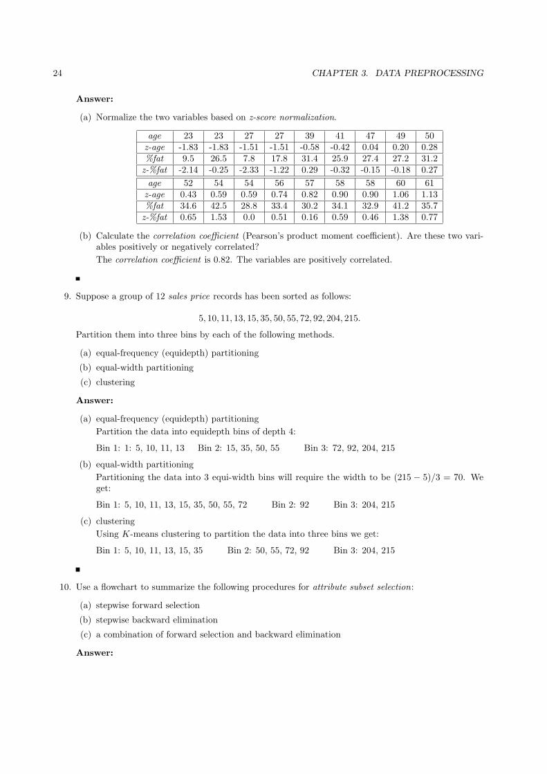
8. Using the data for age and body fat given in Exercise 2.4, answer the following:
(a) Normalize the two attributes based on z-score normalization.
(b) Calculate the correlation coefficient (Pearson’s product moment coefficient). Are these two at-tributes positively or negatively correlated? Compute their covariance.
24 CHAPTER 3. DATA PREPROCESSING
Answer:
(a) Normalize the two variables based on z-score normalization.
age 23 23 27 27 39 41 47 49 50z-age -1.83 -1.83 -1.51 -1.51 -0.58 -0.42 0.04 0.20 0.28%fat 9.5 26.5 7.8 17.8 31.4 25.9 27.4 27.2 31.2z-%fat -2.14 -0.25 -2.33 -1.22 0.29 -0.32 -0.15 -0.18 0.27
age 52 54 54 56 57 58 58 60 61z-age 0.43 0.59 0.59 0.74 0.82 0.90 0.90 1.06 1.13%fat 34.6 42.5 28.8 33.4 30.2 34.1 32.9 41.2 35.7z-%fat 0.65 1.53 0.0 0.51 0.16 0.59 0.46 1.38 0.77
(b) Calculate the correlation coefficient (Pearson’s product moment coefficient). Are these two vari-ables positively or negatively correlated?
The correlation coefficient is 0.82. The variables are positively correlated.
9. Suppose a group of 12 sales price records has been sorted as follows:
5, 10, 11, 13, 15, 35, 50, 55, 72, 92, 204, 215.
Partition them into three bins by each of the following methods.
(a) equal-frequency (equidepth) partitioning
(b) equal-width partitioning
(c) clustering
Answer:
(a) equal-frequency (equidepth) partitioning
Partition the data into equidepth bins of depth 4:
Bin 1: 1: 5, 10, 11, 13 Bin 2: 15, 35, 50, 55 Bin 3: 72, 92, 204, 215
(b) equal-width partitioning
Partitioning the data into 3 equi-width bins will require the width to be (215 − 5)/3 = 70. Weget:
Bin 1: 5, 10, 11, 13, 15, 35, 50, 55, 72 Bin 2: 92 Bin 3: 204, 215
(c) clustering
Using K-means clustering to partition the data into three bins we get:
Bin 1: 5, 10, 11, 13, 15, 35 Bin 2: 50, 55, 72, 92 Bin 3: 204, 215
10. Use a flowchart to summarize the following procedures for attribute subset selection:
(a) stepwise forward selection
(b) stepwise backward elimination
(c) a combination of forward selection and backward elimination
Answer:

3.1. EXERCISES 25
Figure 3.1: Stepwise forward selection.
(a) Stepwise forward selection
See Figure 3.1.
(b) Stepwise backward elimination
See Figure 3.2.
(c) A combination of forward selection and backward elimination
See Figure 3.3.
11. Using the data for age given in Exercise 3.3,
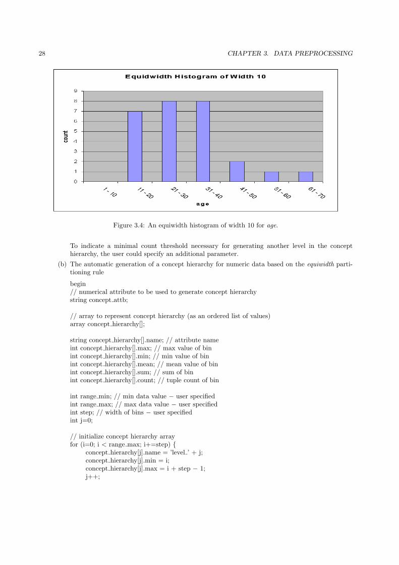
(a) Plot an equal-width histogram of width 10.
(b) Sketch examples of each of the following sampling techniques: SRSWOR, SRSWR, cluster sam-pling, stratified sampling. Use samples of size 5 and the strata “youth”, “middle-aged”, and“senior”.
Answer:
(a) Plot an equiwidth histogram of width 10.
See Figure 3.4.
(b) Sketch examples of each of the following sampling techniques: SRSWOR, SRSWR, cluster sam-pling, stratified sampling. Use samples of size 5 and the strata “young”, “middle-aged”, and“senior”.
See Figure 3.5.
12. ChiMerge [Ker92] is a supervised, bottom-up (i.e., merge-based) data discretization method. It relieson χ2 analysis: adjacent intervals with the least χ2 values are merged together till the chosen stoppingcriterion satisfies.

26 CHAPTER 3. DATA PREPROCESSING
Figure 3.2: Stepwise backward elimination.
(a) Briefly describe how ChiMerge works.
(b) Take the IRIS data set, obtained from the UC-Irvine Machine Learning Data Repository(http://www.ics.uci.edu/∼mlearn/MLRepository.html), as a data set to be discretized. Performdata discretization for each of the four numerical attributes using the ChiMerge method. (Let thestopping criteria be: max-interval = 6). You need to write a small program to do this to avoidclumsy numerical computation. Submit your simple analysis and your test results: split points,final intervals, and your documented source program.
Answer:
(a) The ChiMerge algorithm consists of an initialization step and a bottom-up merging process, whereintervals are continuously merged until a termination condition is met. Chimerge is initialized byfirst sorting the training examples according to their value for the attribute being discretized andthen constructing the initial discretization, in which each example is put into its own interval (i.e.,place an interval boundary before and after each example). The interval merging process containstwo steps, repeated continuously: (1) compute the χ2 value for each pair of adjacent intervals, (2)merge (combine) the pair of adjacent intervals with the lowest χ2 value. Merging continues untila predefined stopping criterion is met.
(b) According to the description in (a), the ChiMerge algorithm can be easily implemented. Detailedempirical results and discussions can be found in this paper: Kerber, R. (1992). ChiMerge :Discretization of numeric attributes, In Proceedings of the Tenth National Conference on ArtificialIntelligence, 123-128.
13. Propose an algorithm, in pseudocode or in your favorite programming language, for the following:
(a) The automatic generation of a concept hierarchy for categorical data based on the number ofdistinct values of attributes in the given schema
(b) The automatic generation of a concept hierarchy for numerical data based on the equal-widthpartitioning rule

3.1. EXERCISES 27
Figure 3.3: A combination of forward selection and backward elimination.
(c) The automatic generation of a concept hierarchy for numerical data based on the equal-frequencypartitioning rule
Answer:
(a) The automatic generation of a concept hierarchy for categorical data based on the number ofdistinct values of attributes in the given schema
Pseudocode for the automatic generation of a concept hierarchy for categorical data based on thenumber of distinct values of attributes in the given schema:
begin// array to hold name and distinct value count of attributes// used to generate concept hierarchyarray count ary[]; string count ary[].name; // attribute nameint count ary[].count; // distinct value count
// array to represent concept hierarchy (as an ordered list of values)array concept hierarchy[];
for each attribute ’A’ in schema {distinct count = count distinct ’A’;insert (’A’, ’distinct count’) into count ary[];
}
sort count ary[] ascending by count;
for (i = 0; i < count ary[].length; i++) {// generate concept hierarchy nodes
concept hierarchy[i] = count ary[i].name;} end
28 CHAPTER 3. DATA PREPROCESSING
Figure 3.4: An equiwidth histogram of width 10 for age.
To indicate a minimal count threshold necessary for generating another level in the concepthierarchy, the user could specify an additional parameter.
(b) The automatic generation of a concept hierarchy for numeric data based on the equiwidth parti-tioning rule
begin// numerical attribute to be used to generate concept hierarchystring concept attb;
// array to represent concept hierarchy (as an ordered list of values)array concept hierarchy[];
string concept hierarchy[].name; // attribute nameint concept hierarchy[].max; // max value of binint concept hierarchy[].min; // min value of binint concept hierarchy[].mean; // mean value of binint concept hierarchy[].sum; // sum of binint concept hierarchy[].count; // tuple count of bin
int range min; // min data value − user specifiedint range max; // max data value − user specifiedint step; // width of bins − user specifiedint j=0;
// initialize concept hierarchy arrayfor (i=0; i < range max; i+=step) {
concept hierarchy[j].name = ’level ’ + j;concept hierarchy[j].min = i;concept hierarchy[j].max = i + step − 1;j++;

3.1. EXERCISES 29
}
// initialize final max value if necessaryif (i ≥ range max) {
concept hierarchy[j].max = i + step − 1;}
// assign each value to a bin by incrementing the appropriate sum and count valuesfor each tuple T in task relevant data set {
int k=0;while (T.concept attb > concept hierarchy[k].max) { k++; }concept hierarchy[k].sum += T.concept attb;concept hierarchy[k].count++;
}
// calculate the bin metric used to represent the value of each level// in the concept hierarchyfor i=0; i < concept hierarchy[].length; i++) {
concept hierarchy[i].mean = concept hierarchy[i].sum / concept hierarchy[i].count;} endThe user can specify more meaningful names for the concept hierarchy levels generated by review-ing the maximum and minimum values of the bins, with respect to background knowledge aboutthe data (i.e., assigning the labels young, middle-aged and old to a three level hierarchy generatedfor age.) Also, an alternative binning method could be implemented, such as smoothing by binmodes.
(c) The automatic generation of a concept hierarchy for numeric data based on the equidepth parti-tioning rule
Pseudocode for the automatic generation of a concept hierarchy for numeric data based on theequidepth partitioning rule:
begin// numerical attribute to be used to generate concept hierarchystring concept attb;
// array to represent concept hierarchy (as an ordered list of values)array concept hierarchy[];string concept hierarchy[].name; // attribute nameint concept hierarchy[].max; // max value of binint concept hierarchy[].min; // min value of binint concept hierarchy[].mean; // mean value of binint concept hierarchy[].sum; // sum of binint concept hierarchy[].count; // tuple count of bin
int bin depth; // depth of bins to be used − user specifiedint range min; // min data value − user specifiedint range max; // max data value − user specified
// initialize concept hierarchy arrayfor (i=0; i < (range max/bin depth(; i++) {
concept hierarchy[i].name = ’level ’ + i;concept hierarchy[i].min = 0;

30 CHAPTER 3. DATA PREPROCESSING
concept hierarchy[i].max = 0;}
// sort the task-relevant data set sort data set ascending by concept attb;
int j=1; int k=0;
// assign each value to a bin by incrementing the appropriate sum,// min and max values as necessaryfor each tuple T in task relevant data set {
concept hierarchy[k].sum += T.concept attb;concept hierarchy[k].count++;if (T.concept attb <= concept hierarchy[k].min) {
concept hierarchy[k].min = T.concept attb;}if (T.concept attb >= concept hierarchy[k].max) {
concept hierarchy[k].max = T.concept attb;};j++;if (j > bin depth) {
k++; j=1;}
}
// calculate the bin metric used to represent the value of each level// in the concept hierarchyfor i=0; i < concept hierarchy[].length; i++) {
concept hierarchy[i].mean = concept hierarchy[i].sum / concept hierarchy[i].count;}end
This algorithm does not attempt to distribute data values across multiple bins in order to smoothout any difference between the actual depth of the final bin and the desired depth to be imple-mented. Also, the user can again specify more meaningful names for the concept hierarchy levelsgenerated by reviewing the maximum and minimum values of the bins, with respect to backgroundknowledge about the data.
14. Robust data loading poses a challenge in database systems because the input data are often dirty.In many cases, an input record may miss multiple values, some records could be contaminated, withsome data values out of range or of a different data type than expected. Work out an automated datacleaning and loading algorithm so that the erroneous data will be marked, and contaminated data willnot be mistakenly inserted into the database during data loading.
Answer:
We can tackle this automated data cleaning and loading problem from the following perspectives:
• Use metadata (e.g., domain, range, dependency, distribution).
• Check unique rule, consecutive rule and null rule.
• Check field overloading.
• Spell-checking.

3.2. SUPPLEMENTARY EXERCISES 31
• Detect different attribute names which actually have the same meaning.
• Use domain knowledge to detect errors and make corrections.
3.2 Supplementary Exercises
1. The following table contains the attributes name, gender, trait-1, trait-2, trait-3, and trait-4, wherename is an object identifier, gender is a symmetric attribute, and the remaining trait attributes areasymmetric, describing personal traits of individuals who desire a penpal. Suppose that a service existsthat attempts to find pairs of compatible penpals.
name gender trait-1 trait-2 trait-3 trait-4
Kevin M N P P NCaroline F N P P NErik M P N N P...
......
......
...
2MKJiawei, can we please discuss this exercise? There are many ambiguities.
For asymmetric attribute values, let the value P be set to 1 and the value N be set to 0. Suppose thatthe distance between objects (potential penpals) is computed based only on the asymmetric variables.
(a) Show the contingency matrix for each pair given Kevin, Caroline, and Erik (based on trait-1 totrait-4 ).
(b) 2MKBased on our discussion, we no longer refer to simple matching coefficient or Jaccard co-efficient in Section 7.2.2. Compute the invariant dissimilarity of each pair using Equation (??).2MKAmbiguity: Why does part (b) use the equation for symmetric binary variables when weinstruct the reader to use only the four asymmetric variables? Note that the answers we get forparts (b) and (c) are even identical, so I see no point in asking this confusing question??
(c) Compute the noninvariant dissimilarity of each pair using Equation (??).
(d) Who do you suggest would make the best pair of penpals? Which pair of individuals would bethe least compatible?
(e) Suppose that we are to include the symmetric variable gender in our analysis. Based on Equa-tion (??), who would be the most compatible pair, and why?
2MKAmbiguity: Why are we asking the reader to use the Equation for assymetric variables whenincluding the symmetric variable gender? (and if so, we would need to specify whether M or Fshould be coded as 1)? Shouldn’t they be using the technique for variables of mixed types? Ilooked at my copy of the answer book and, based on the calculations, it does appear that theequation for variables of mixed type is used (which contradicts our question). However, I obtaindifferent answers than in the answer book (although my copy may be outdated.) I obtained d(K,C)= 1/1 = 1 (disagrees with answer book); d(K,E) = 4/5 (agrees with answer book); d(C,E) = 5/5= 1 (different derivation than answer book). Let’s discuss! Thanks.

32 CHAPTER 3. DATA PREPROCESSING
TuplesT1 13T2 15T3 16T4 16T5 19T6 20T7 20T8 21T9 22
T10 22T11 25T12 25T13 25T14 25T15 30T16 33T17 33T18 33
T19 33T20 35T21 35T22 36T23 40T24 45T25 46T26 52T27 70
SRSWOR vs. SRSWR
SRSWOR (n = 5)
T4 16T6 20T10 22T11 25T26 32
SRSWR (n = 5)
T7 20T7 20T20 35T21 35T25 46
Clustering sampling: Initial clustersT1 13T2 15T3 16T4 16T5 19
T6 20T7 20T8 21T9 22T10 22
T11 25T12 25T13 25T14 25T15 30
T16 33T17 33T18 33T19 33T20 35
T21 35T22 36T23 40T24 45T25 46
T26 52T27 70
Cluster sampling (m = 2)
T6 20T7 20T8 21T9 22T10 22
T21 35T22 36T23 40T24 45T25 46
Stratified SamplingT1 13 youngT2 15 youngT3 16 youngT4 16 youngT5 19 youngT6 20 youngT7 20 youngT8 21 youngT9 22 young
T10 22 youngT11 25 youngT12 25 youngT13 25 youngT14 25 youngT15 30 middle ageT16 33 middle ageT17 33 middle ageT18 33 middle age
T19 33 middle ageT20 35 middle ageT21 35 middle ageT22 36 middle ageT23 40 middle ageT24 45 middle ageT25 46 middle ageT26 52 middle ageT27 70 senior
Stratified Sampling (according to age)
T4 16 youngT12 25 youngT17 33 middle ageT25 46 middle ageT27 70 senior
Figure 3.5: Examples of sampling: SRSWOR, SRSWR, cluster sampling, stratified sampling.

Chapter 4
Data Warehousing and OnlineAnalytical Processing
4.1 Exercises
1. State why, for the integration of multiple heterogeneous information sources, many companies in in-dustry prefer the update-driven approach (which constructs and uses data warehouses), rather thanthe query-driven approach (which applies wrappers and integrators). Describe situations where thequery-driven approach is preferable over the update-driven approach.
Answer:
For decision-making queries and frequently-asked queries, the update-driven approach is more prefer-able. This is because expensive data integration and aggregate computation are done before queryprocessing time. In order for the data collected in multiple heterogeneous databases to be used indecision-making processes, data must be integrated and summarized with the semantic heterogeneityproblems among multiple databases analyzed and solved. If the query-driven approach is employed,these queries will be translated into multiple (often complex) queries for each individual database. Thetranslated queries will compete for resources with the activities at the local sites, thus degrading theirperformance. In addition, these queries will generate a complex answer set, which will require furtherfiltering and integration. Thus, the query-driven approach is, in general, inefficient and expensive.The update-driven approach employed in data warehousing is faster and more efficient since a lot ofprecomputation could be done off-line.
For queries that are used rarely, reference the most current data, and/or do not require aggregations,the query-driven approach would be preferable over the update-driven approach. In this case, it maynot be justifiable for an organization to pay heavy expenses for building and maintaining a datawarehouse, if only a small number and/or relatively small size databases are used; or if the queries relyon the current data, since the data warehouses do not contain the most current information.
2. Briefly compare the following concepts. You may use an example to explain your point(s).
(a) Snowflake schema, fact constellation, starnet query model
(b) Data cleaning, data transformation, refresh
(c) Discovery-driven cube, multifeature cube, virtual warehouse
Answer:
33

34 CHAPTER 4. DATA WAREHOUSING AND ONLINE ANALYTICAL PROCESSING
(a) Snowflake schema, fact constellation, starnet query model
The snowflake schema and fact constellation are both variants of the star schema model, whichconsists of a fact table and a set of dimension tables; the snowflake schema contains somenormalized dimension tables, whereas the fact constellation contains a set of fact tables thatshare some common dimension tables. A starnet query model is a query model (not a schemamodel), which consists of a set of radial lines emanating from a central point, where each radialline represents one dimension and each point (called a “footprint”) along the line represents alevel of the dimension, and these “footprints” represent the granularity available for use by OLAPoperations such as drill-down and roll-up. The starnet query model, as suggested by its name, isused for querying and provides users with a global view of OLAP operations.
(b) Data cleaning, data transformation, refresh
Data cleaning is the process of detecting errors in the data and rectifying them when possible.Data transformation is the process of converting the data from heterogeneous sources to aunified data warehouse format or semantics. Refresh is the function propagating the updatesfrom the data sources to the warehouse.
(c) Discovery-driven cube, multi-feature cube, virtual warehouse
A discovery-driven cube uses precomputed measures and visual cues to indicate data exceptionsat all levels of aggregation, guiding the user in the data analysis process. A multi-feature cubecomputes complex queries involving multiple dependent aggregates at multiple granularities (e.g.,to find the total sales for every item having a maximum price, we need to apply the aggregatefunction SUM to the tuple set output by the aggregate function MAX). A virtual warehouse is aset of views (containing data warehouse schema, dimension, and aggregate measure definitions)over operational databases.
3. Suppose that a data warehouse consists of the three dimensions time, doctor, and patient, and the twomeasures count and charge, where charge is the fee that a doctor charges a patient for a visit.
(a) Enumerate three classes of schemas that are popularly used for modeling data warehouses.
(b) Draw a schema diagram for the above data warehouse using one of the schema classes listed in (a).
(c) Starting with the base cuboid [day, doctor, patient], what specific OLAP operations should beperformed in order to list the total fee collected by each doctor in 2004?
(d) To obtain the same list, write an SQL query assuming the data is stored in a relational databasewith the schema fee (day, month, year, doctor, hospital, patient, count, charge).
Answer:
(a) Enumerate three classes of schemas that are popularly used for modeling data warehouses.
Three classes of schemas popularly used for modeling data warehouses are the star schema, thesnowflake schema, and the fact constellation schema.
(b) Draw a schema diagram for the above data warehouse using one of the schema classes listed in(a).
A star schema is shown in Figure 4.1.
(c) Starting with the base cuboid [day, doctor, patient], what specific OLAP operations should beperformed in order to list the total fee collected by each doctor in 2010?
The operations to be performed are:
• Roll-up on time from day to year.
• Slice for time = 2010.
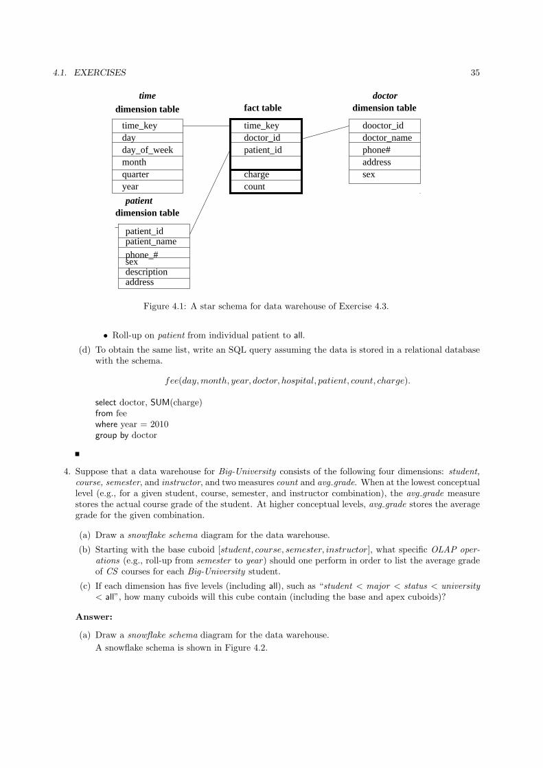
4.1. EXERCISES 35
time_keydayday_of_weekmonthquarteryear
dimension tabletime
dimension tablepatient
sexdescriptionaddress
phone_#
patient_namepatient_id
time_key
patient_id
chargecount
doctor_id
fact table dimension tabledoctor
dooctor_iddoctor_namephone#addresssex
Figure 4.1: A star schema for data warehouse of Exercise 4.3.
• Roll-up on patient from individual patient to all.
(d) To obtain the same list, write an SQL query assuming the data is stored in a relational databasewith the schema.
fee(day,month, year, doctor, hospital, patient, count, charge).
select doctor, SUM(charge)from feewhere year = 2010group by doctor
4. Suppose that a data warehouse for Big-University consists of the following four dimensions: student,course, semester, and instructor, and two measures count and avg grade. When at the lowest conceptuallevel (e.g., for a given student, course, semester, and instructor combination), the avg grade measurestores the actual course grade of the student. At higher conceptual levels, avg grade stores the averagegrade for the given combination.
(a) Draw a snowflake schema diagram for the data warehouse.
(b) Starting with the base cuboid [student, course, semester, instructor], what specific OLAP oper-ations (e.g., roll-up from semester to year) should one perform in order to list the average gradeof CS courses for each Big-University student.
(c) If each dimension has five levels (including all), such as “student < major < status < university< all”, how many cuboids will this cube contain (including the base and apex cuboids)?
Answer:
(a) Draw a snowflake schema diagram for the data warehouse.
A snowflake schema is shown in Figure 4.2.

36 CHAPTER 4. DATA WAREHOUSING AND ONLINE ANALYTICAL PROCESSING
semester_id
year
dimension tablesemester
semesterinstructor
deptrank
dimension table
instructor_id
student_idcourse_id
instructor_idcountavg_grade
student_idstudent_name
status
dimension table
course_idcourse_name
fact tableuniv
dimension tablestudent
semester_id
coursedimension table
area
cityprovincecountry
area_id
majorarea_id
university
department
Figure 4.2: A snowflake schema for data warehouse of Exercise 4.4.
(b) Starting with the base cuboid [student, course, semester, instructor], what specific OLAP opera-tions (e.g., roll-up from semester to year) should one perform in order to list the average grade ofCS courses for each Big-University student.
The specific OLAP operations to be performed are:
• Roll-up on course from course id to department.
• Roll-up on semester from semester id to all.
• Slice for course=“CS” .
(c) If each dimension has five levels (including all), such as student < major < status < university <all, how many cuboids will this cube contain (including the base and apex cuboids)?
This cube will contain 54 = 625 cuboids.
5. Suppose that a data warehouse consists of the four dimensions, date, spectator, location, and game,and the two measures, count and charge, where charge is the fare that a spectator pays when watchinga game on a given date. Spectators may be students, adults, or seniors, with each category having itsown charge rate.
(a) Draw a star schema diagram for the data warehouse.
(b) Starting with the base cuboid [date, spectator, location, game], what specific OLAP operationsshould one perform in order to list the total charge paid by student spectators at GM Place in2010?
(c) Bitmap indexing is useful in data warehousing. Taking this cube as an example, briefly discussadvantages and problems of using a bitmap index structure.
Answer:
(a) Draw a star schema diagram for the data warehouse.
A star schema is shown in Figure 4.3.

4.1. EXERCISES 37
dimension tabledate
date_iddaymonth
quarter
year
fact tablesales
dimension table
date_idspectator_idgame_idlocation_idcountcharge
dimension tablegame
game_idgame_namedescriptionproducer
spectator
spectator_id
spectator_namestatus
phone
address
locationdimension table
location_idlocation_namephone#streetcity
provincecountry
Figure 4.3: A star schema for data warehouse of Exercise 4.5.
(b) Starting with the base cuboid [date, spectator, location, game], what specific OLAP operationsshould one perform in order to list the total charge paid by student spectators at GM Place in2010?
The specific OLAP operations to be performed are:
• Roll-up on date from date id to year.
• Roll-up on game from game id to all.
• Roll-up on location from location id to location name.
• Roll-up on spectator from spectator id to status.
• Dice with status=“students”, location name=“GM Place”, and year = 2010.
(c) Bitmap indexing is useful in data warehousing. Taking this cube as an example, briefly discussadvantages and problems of using a bitmap index structure.
Bitmap indexing is advantageous for low-cardinality domains. For example, in this cube, if di-mension location is bitmap indexed, comparison, join, and aggregation operations over locationare then reduced to bit arithmetic, which substantially reduces the processing time. Further-more, strings of long location names can be represented by a single bit, which leads to significantreduction in space and I/O. For dimensions with high-cardinality, such as date in this example,the vector to present the bitmap index could be very long. For example, a 10-year collection ofdata could result in 3650 data records, meaning that every tuple in the fact table would require3650 bits, or approximately 456 bytes, to hold the bitmap index. However, using bit-vectorcompression techniques can overcome this difficulty to a certain degree.
6. A data warehouse can be modeled by either a star schema or a snowflake schema. Briefly describe thesimilarities and the differences of the two models, and then analyze their advantages and disadvantageswith regard to one another. Give your opinion of which might be more empirically useful and statethe reasons behind your answer.
Answer:

38 CHAPTER 4. DATA WAREHOUSING AND ONLINE ANALYTICAL PROCESSING
They are similar in the sense that they all have a fact table, as well as some dimensional tables.The major difference is that some dimension tables in the snowflake schema are normalized, therebyfurther splitting the data into additional tables. The advantage for star schema is its simplicity, whichwill enable efficiency, but it requires more space. For snowflake schema, it reduces some redundancyby sharing common tables: The tables are easy to maintain and save some space. However, it is lessefficient, and the saving of space is negligible in comparison with the typical magnitude of the fact table.Therefore, empirically, star schema is more popular because nowadays, efficiency has higher priorityover space, if it is not too huge. Sometimes in industry, to speed up processing, people “denormalizedata from a snowflake schema into a star schema” [1]. Another option here is that “some practitionersuse a snowflake schema to maintain dimensions, and then present users with the same data collapsedinto a star” [2].
Some references for the answer to this question: Oracle Tip: Understand the difference between starand snowflake schemas in OLAP.
[1] http://builder.com.com/5100-6388-5221690.html Star vs. Snowflake Schemas.
[2] http://blogs.msdn.com/bi systems/articles/164525.aspx
7. Design a data warehouse for a regional weather bureau. The weather bureau has about 1,000 probes,which are scattered throughout various land and ocean locations in the region to collect basic weatherdata, including air pressure, temperature, and precipitation at each hour. All data are sent to thecentral station, which has collected such data for over 10 years. Your design should facilitate efficientquerying and online analytical processing, and derive general weather patterns in multidimensionalspace.
Answer:
Since the weather bureau has about 1000 probes scattered throughout various land and ocean locations,we need to construct a spatial data warehouse so that a user can view weather patterns on a map bymonth, by region, and by different combinations of temperature and precipitation, and can dynamicallydrill down or roll up along any dimension to explore desired patterns.
The star schema of this weather spatial data warehouse can be constructed as shown in Figure 4.4.
To construct this spatial data warehouse, we may need to integrate spatial data from heterogeneoussources and systems. Fast and flexible online analytical processing in spatial data warehouse is animportant factor. There are three types of dimensions in a spatial data cube: nonspatial dimensions,spatial-to-nonspatial dimensions, and spatial-to-spatial dimensions. We distinguish two types of mea-sures in a spatial data cube: numerical measures and spatial measures. A nonspatial data cube containsonly nonspatial dimensions and numerical measures. If a spatial data cube contains spatial dimensionsbut no spatial measures, then its OLAP operations (such as drilling or pivoting) can be implemented ina manner similar to that of nonspatial data cubes. If a user needs to use spatial measures in a spatialdata cube, we can selectively precompute some spatial measures in the spatial data cube. Which por-tion of the cube should be selected for materialization depends on the utility (such as access frequencyor access priority), sharability of merged regions, and the balanced overall cost of space and onlinecomputation.
8. A popular data warehouse implementation is to construct a multidimensional database, known as adata cube. Unfortunately, this may often generate a huge, yet very sparse multidimensional matrix.
(a) Present an example illustrating such a huge and sparse data cube.
(b) Design an implementation method that can elegantly overcome this sparse matrix problem. Notethat you need to explain your data structures in detail and discuss the space needed, as well ashow to retrieve data from your structures.

4.1. EXERCISES 39
temperaturetemp_rangetemp_description
temperaturedimension table
daymonth
quarter
year
time
dimension tableprecipitation
prec_description
prec_range
fact table dimension tabledimension tabledate weather
timeregiontemperatureprecipitationregion_maparea
region
location_idprobe_location
county
city
region_name
province
district
precipitation
Figure 4.4: A star schema for a weather spatial data warehouse of Exercise 4.7.
(c) Modify your design in (b) to handle incremental data updates. Give the reasoning behind yournew design.
Answer:
(a) Present an example illustrating such a huge and sparse data cube.
An example of a huge and sparse data cube can be one that is generated from a telephonecompany billing database that keeps records on each customer’s billing information, such ascontact information, payment methods, date of payment, and detailed call records. For thetelephone company, it would be very expensive to keep detailed call records for every customerfor longer than three months. Therefore, it would be beneficial to remove that information fromthe database, keeping only the total number of calls made, the total minutes billed, and theamount billed, for example. The resulting computed data cube for the billing database wouldhave large amounts of missing or removed data, resulting in a huge and sparse data cube.
(b) Design an implementation method that can elegantly overcome this sparse matrix problem. Notethat you need to explain your data structures in detail and discuss the space needed, as well ashow to retrieve data from your structures.
A way to overcome the sparse matrix problem is to use multiway array aggregation. (Note:this answer is based on the paper, Y. Zhao, P. M. Deshpande, and J. F. Naughton, “An array-based algorithm for simultaneous multidimensional aggregates”, in Proc. 1997 ACM-SIGMODInt. Conf. Management of Data, pages 159–170, Tucson, Arizona, May 1997).
The first step consists of partitioning the array-based cube into chunks, or subcubes that aresmall enough to fit into the available memory for cube computation. Each of these chunks isfirst compressed to remove cells that do not contain any valid data, and is then stored as anobject on disk. For storage and retrieval purposes, the “chunkID + offset” can be used as thecell address. The second step involves computing the aggregates by visiting cube cells in an orderthat minimizes the number of times that each cell must be revisited, thereby reducing memoryaccess and storage costs. By first sorting and computing the planes of the data cube accordingto their size in ascending order, a smaller plane can be kept in main memory while fetching andcomputing only one chunk at a time for a larger plane.

40 CHAPTER 4. DATA WAREHOUSING AND ONLINE ANALYTICAL PROCESSING
(c) Modify your design in (b) to handle incremental data updates. Give the reasoning behind yournew design.
In order to handle incremental data updates, the data cube is first computed as described in (b).Then only the chunk that contains the cells with the new data is recomputed without needingto recompute the entire cube. This is because, with incremental updates, only one chunk at atime can be affected. Then the recomputed value needs to be propagated to its correspondinghigher-level cuboids. Thus, incremental data updates can be performed efficiently.
9. Regarding the computation of measures in a data cube:
(a) Enumerate three categories of measures, based on the kind of aggregate functions used in com-puting a data cube.
(b) For a data cube with the three dimensions time, location, and item, which category does thefunction variance belong to? Describe how to compute it if the cube is partitioned into manychunks.
Hint: The formula for computing variance is 1N
∑Ni=1(xi − xi)
2, where xi is the average of xis.
(c) Suppose the function is “top 10 sales.” Discuss how to efficiently compute this measure in a datacube.
Answer:
(a) Enumerate three categories of measures, based on the kind of aggregate functions used in com-puting a data cube.
The three categories of measures are distributive, algebraic, and holistic.
(b) For a data cube with three dimensions: time, location, and product, which category does thefunction variance belong to? Describe how to compute it if the cube is partitioned into manychunks.
Hint: The formula for computing variance is 1n
∑ni=1(xi)
2 − xi2, where xi is the average of xi’s.
The function variance is algebraic. If the cube is partitioned into many chunks, the variance canbe computed as follows: Read in the chunks one by one, keeping track of the accumulated (1)number of tuples, (2) sum of (xi)
2, and (3) sum of xi. After reading all the chunks, compute theaverage of xi’s as the sum of xi divided by the total number of tuples. Use the formula as shownin the hint to get the variance.
(c) Suppose the function is “top 10 sales.” Discuss how to efficiently compute this measure in a datacube.
For each cuboid, use 10 units to register the top 10 sales found so far. Read the data in eachcubiod once. If the sales amount in a tuple is greater than an existing one in the top-10 list,insert the new sales amount from the new tuple into the list, and discard the smallest one in thelist. The computation of a higher level cuboid can be performed similarly by propagation of thetop-10 cells of its corresponding lower level cuboids.
10. Suppose a company would like to design a data warehouse to facilitate the analysis of moving vehiclesin an online analytical processing manner. The company registers huge amounts of auto movementdata in the format of (Auto ID, location, speed, time). Each Auto ID represents a vehicle associatedwith information, such as vehicle category, driver category, etc., and each location may be associatedwith a street in a city. Assume that a street map is available for the city.

4.1. EXERCISES 41
(a) Design such a data warehouse to facilitate effective online analytical processing in multidimen-sional space.
(b) The movement data may contain noise. Discuss how you would develop a method to automaticallydiscover data records that were likely erroneously registered in the data repository.
(c) The movement data may be sparse. Discuss how you would develop a method that constructs areliable data warehouse despite the sparsity of data.
(d) If one wants to drive from A to B starting at a particular time, discuss how a system may use thedata in this warehouse to work out a fast route for the driver.
Answer:
(a) Design such a data warehouse to facilitate effective online analytical processing in multidimen-sional space.
To design a data warehouse for the analysis of moving vehicles, we can consider vehicle as afact table that points to four dimensions: auto, time, location and speed. The measures canvary depending on the desired target and the power required. Here, measures considered arevehicle sold and vehicle mileage.
A star schema is shown in Figure 4.5.
Figure 4.5: A star schema for data warehouse of Exercise 4.10.
(b) The movement data may contain noise. Discuss how you would develop a method to automaticallydiscover data records that were likely erroneously registered in the data repository.
To handle the noise in data, we first need to do data cleaning. Missing values may be filledor dropped entirely, depending on the tolerance of the system. Then we can use some datasmoothing techniques to remove noisy data points, for example, regression and outlier analysis.Finally, we can also set up some rules to detect inconsistent data and remove them based ondomain knowledge.
(c) The movement data may be sparse. Discuss how you would develop a method that constructs areliable data warehouse despite the sparsity of data.

42 CHAPTER 4. DATA WAREHOUSING AND ONLINE ANALYTICAL PROCESSING
It may be possible to get a data in the data warehouse that may be sparse. Analyzing a sparsedata is not reliable as a single outlier may completely shift the results. Hence there are fewefficient values to deal with it. We have to evaluate the confidence interval in such case whereconfidence interval is a measure that defines the reliability of the data. Smaller the confidenceinterval, better it is. If the confidence interval is too large this indicates larger ambiguity in thedata. Hence, for our vehicle database we can compute confidence interval. Confidence intervalcan be large in an example like when data size was large enough, but the queried data cell hadonly few or no values. In such a case, we have 2 ways to resolve this issue:
Intra-cuboid query: Expand the sample size by including the nearby cells in the same cuboid asthe queried cellthat reduces the confidence interval.
Inter-cuboid query: It is the extreme case of intra-cuboid. In this remove the dimension bygeneralizing it. Also, sparsity can be considered as a missing value. We may use the existingdata to find that missing value. This technique is most commonly used in machine learning. E.g.if speed is missing, then we can view speed as per a function of location or time. Hence, speedrecorded previously on that particular street and that particular time may be considered insteadof that missing value. Provided the semantics of the query is not change, we can even reducethe dimensionality of the data cube. Hence, if some cell was sparse at a query execution for aparticular hour, we may generalize it to a day. This may now give some values in that cell.
(d) If one wants to drive from A to B starting at a particular time, discuss how a system may use thedata in this warehouse to work out a fast route for the driver.
Using this warehouse, we can look up the information for those vehicles of the same vehiclecategory and driver category. Then using OLAP operation (drill, dice,..) we look up for the speedof a location at a specific time (atlevel of hour) and will use that as the weight for the streeton the city graph. We need to find the weight for allthe possible paths from the start locationto end location. Using this weighted graph we can work out the fastest route for the driver byany famous algorithm such as A* and Dijktra. We might need to update the weights everyhour.Using this algorithm, we don’t care about the direction of the street. We can also integrated thatinformation and create a directed graph. Based on the graph, we can calculate the fastest route.
11. RFID (Radio-frequency identification) is commonly used to trace object movement and perform in-ventory control. An RFID reader can successfully read an RFID tag from a limited distance at anyscheduled time. Suppose a company would like to design a data warehouse to facilitate the analysis ofobjects with RFID tags in an online analytical processing manner. The company registers huge amountsof RFID data in the format of (RFID, at location, time), and also has some information about theobjects carrying the RFID tag, e.g., (RFID, product name, product category, producer, date produced,price).
(a) Design a data warehouse to facilitate effective registration and online analytical processing of suchdata.
(b) The RFID data may contain lots of redundant information. Discuss a method that maximallyreduces redundancy during data registration in the RFID data warehouse.
(c) The RFID data may contain lots of noise, such as missing registration and misreading of IDs.Discuss a method that effectively cleans up the noisy data in the RFID data warehouse.
(d) One may like to perform online analytical processing to determine how many TV sets were shippedfrom the LA seaport to BestBuy in Champaign, Illinois by month, by brand, and by price range.Outline how this can be done efficiently if you were to store such RFID data in the warehouse.
(e) If a customer returns a jug of milk and complains that is has spoiled before its expiration data,discuss how you could investigate such a case in the warehouse to find out what could be theproblem, either in shipping or in storage.

4.1. EXERCISES 43
Answer:
(a) Design a data warehouse to facilitate effective registration and online analytical processing of suchdata.
A RFID warehouse need to contains a fact table, stay, composed of cleansed RFID records; aninformation table, info, that stores path-independent information for each item; and a map tablethat links together different records in the fact table that form a path. The main differencebetween the RFID warehouse and a traditional warehouse is the presence of the map table linkingrecords from the fact table (stay) in order to preserve the original structure of the data.
A star schema is shown in Figure 4.6.
Figure 4.6: A star schema for data warehouse of Exercise 4.11.
(b) The RFID data may contain lots of redundant information. Discuss a method that maximallyreduces redundancy during data registration in the RFID data warehouse.
Each reader provides tuples of the form (RFID; location; time) at xed time intervals. When anitem stays at the same location, for a period of time, multiple tuples will be generated. We cangroup these tuples into a single one of the form (RFID; location; time in; time out). For example,if a supermarket has readers on each shelf that scan the items every minute, and items stay onthe shelf on average for 1 day, we get a 1,440 to 1 reduction in size without loss of information.
(c) The RFID data may contain lots of noise, such as missing registration and misreading of IDs.Discuss a method that effectively cleans up the noisy data in the RFID data warehouse.
One can use the assumption that many RFID objects stay or move together, especially at theearly stage of distribution, or use the historically most likely path for a given item, to infer orinterpolate the miss and error reading.
(d) One may like to perform online analytical processing to determine how many TV sets were shippedfrom the LA seaport to BestBuy in Champaign, Illinois by month, by brand, and by price range.Outline how this can be done efficiently if you were to store such RFID data in the warehouse.
Compute an aggregate measure on the tags that travel through a set of locations and that matcha selection criteria on path independent dimensions

44 CHAPTER 4. DATA WAREHOUSING AND ONLINE ANALYTICAL PROCESSING
(e) If a customer returns a jug of milk and complains that is has spoiled before its expiration data,discuss how you could investigate such a case in the warehouse to find out what could be theproblem, either in shipping or in storage.
For this case, after we obtain the RFID of the milk, we can directly use traditional OLAP opera-tions to get the shipping and storage time efficiently.
Some references for the answer to this question:
[1] Hector Gonzalez, Jiawei Han, and Xiaolei Li, ”FlowCube: Constructuing RFID FlowCubes forMulti-Dimensional Analysis of Commodity Flows”, in Proc. 2006 Int. Conf. on Very Large DataBases (VLDB’06), Seoul, Korea, Sept. 2006.
[2] Hector Gonzalez, Jiawei Han, Xiaolei Li, and Diego Klabjan, ”Warehousing and Analysis of MassiveRFID Data Sets”, in Proc. 2006 Int. Conf. on Data Engineering (ICDE’06), Atlanta, Georgia, April2006.
[3] Jiawei Han, Hector Gonzalez, Xiaolei Li and Diego Klabjan, ”Warehousing and Mining MassiveRFID Data Sets”, (Keynote Speech), 2006 Int. Conf. on Advance Data Mining and Its Applications(ADMA’06), Xi’An, China, Aug. 2006.
12. In many applications, new data sets are incrementally added to the existing large data sets. Thus animportant consideration is whether a measure can be computed efficiently in incremental manner. Usecount, standard deviation, and median as examples to show that a distributive or algebraic measurefacilitates efficient incremental computation, whereas a holistic measure does not.
Answer: appeared in Chapter 2
13. Suppose that we need to record three measures in a data cube: min, average, and median. Designan efficient computation and storage method for each measure given that the cube allows data to bedeleted incrementally (i.e., in small portions at a time) from the cube.
Answer:
For min, keep the ⟨min val, count⟩ pair for each cuboid to register the smallest value and its count.For each deleted tuple, if its value is greater than min val, do nothing. Otherwise, decrement the countof the corresponding node. If a count goes down to zero, recalculate the structure.
For average, keep a pair ⟨sum, count⟩ for each cuboid. For each deleted node N , decrement the countand subtract value N from the sum, and average = sum/count.
For median, keep a small number p of centered values, (e.g. p = 10), plus two counts: up count anddown count. Each removal may change the count or remove a centered value. If the median no longerfalls among these centered values, recalculate the set. Otherwise, the median can be easily calculatedfrom the above set.
14. In data warehouse technology, a multiple dimensional view can be implemented by a relational databasetechnique (ROLAP), or by a multidimensional database technique (MOLAP), or by a hybrid databasetechnique (HOLAP).
(a) Briefly describe each implementation technique.
(b) For each technique, explain how each of the following functions may be implemented:
i. The generation of a data warehouse (including aggregation)
ii. Roll-up
iii. Drill-down

4.1. EXERCISES 45
iv. Incremental updating
Which implementation techniques do you prefer, and why?
Answer:
(a) Briefly describe each implementation technique.
A ROLAP technique for implementing a multiple dimensional view consists of intermediateservers that stand in between a relational back-end server and client front-end tools, thereby us-ing a relational or extended-relational DBMS to store and manage warehouse data, and OLAPmiddleware to support missing pieces. A MOLAP implementation technique consists of servers,which support multidimensional views of data through array-based multidimensional storage en-gines that map multidimensional views directly to data cube array structures. A HOLAP imple-mentation approach combines ROLAP and MOLAP technology, which means that large volumesof detailed data and some very low level aggregations can be stored in a relational database, whilesome high level aggregations are kept in a separate MOLAP store.
(b) For each technique, explain how each of the following functions may be implemented:
i. The generation of a data warehouse (including aggregation)ROLAP: Using a ROLAP server, the generation of a data warehouse can be implementedby a relational or extended-relational DBMS using summary fact tables. The fact tables canstore aggregated data and the data at the abstraction levels indicated by the join keys in theschema for the given data cube.MOLAP: In generating a data warehouse, the MOLAP technique uses multidimensional arraystructures to store data and multiway array aggregation to compute the data cubes.HOLAP: The HOLAP technique typically uses a relational database to store the data andsome low level aggregations, and then uses a MOLAP to store higher-level aggregations.
ii. Roll-upROLAP: To roll-up on a dimension using the summary fact table, we look for the record inthe table that contains a generalization on the desired dimension. For example, to roll-upthe date dimension from day to month, select the record for which the day field contains thespecial value all. The value of the measure field, dollars sold, for example, given in this recordwill contain the subtotal for the desired roll-up.MOLAP: To perform a roll-up in a data cube, simply climb up the concept hierarchy for thedesired dimension. For example, one could roll-up on the location dimension from city tocountry, which is more general.HOLAP: The roll-up using the HOLAP technique will be similar to either ROLAP or MOLAP,depending on the techniques used in the implementation of the corresponding dimensions.
iii. Drill-downROLAP: To drill-down on a dimension using the summary fact table, we look for the record inthe table that contains a generalization on the desired dimension. For example, to drill-downon the location dimension from country to province or state, select the record for which onlythe next lowest field in the concept hierarchy for location contains the special value all. In thiscase, the city field should contain the value all. The value of the measure field, dollars sold,for example, given in this record will contain the subtotal for the desired drill-down.MOLAP: To perform a drill-down in a data cube, simply step down the concept hierarchy forthe desired dimension. For example, one could drill-down on the date dimension from monthto day in order to group the data by day rather than by month.HOLAP: The drill-down using the HOLAP technique is similar either to ROLAP or MOLAPdepending on the techniques used in the implementation of the corresponding dimensions.
iv. Incremental updating

46 CHAPTER 4. DATA WAREHOUSING AND ONLINE ANALYTICAL PROCESSING
OLAP: To perform incremental updating, check whether the corresponding tuple is in thesummary fact table. If not, insert it into the summary table and propagate the result up.Otherwise, update the value and propagate the result up.MOLAP: To perform incremental updating, check whether the corresponding cell is in theMOLAP cuboid. If not, insert it into the cuboid and propagate the result up. Otherwise,update the value and propagate the result up.HOLAP: similar either to ROLAP or MOLAP depending on the techniques used in theimplementation of the corresponding dimensions.
(c) Which implementation techniques do you prefer, and why?
HOLAP is often preferred since it integrates the strength of both ROLAP and MOLAP methodsand avoids their shortcomings—if the cube is quite dense, MOLAP is often preferred. Also, if thedata are sparse and the dimensionality is high, there will be too many cells (due to exponentialgrowth) and, in this case, it is often desirable to compute iceberg cubes instead of materializingthe complete cubes.
15. Suppose that a data warehouse contains 20 dimensions, each with about five levels of granularity.
(a) Users are mainly interested in four particular dimensions, each having three frequently accessedlevels for rolling up and drilling down. How would you design a data cube structure to supportthis preference efficiently?
(b) At times, a user may want to drill through the cube, down to the raw data for one or two particulardimensions. How would you support this feature?
Answer:
(a) Users are mainly interested in four particular dimensions, each having three frequently accessedlevels for rolling up and drilling down. How would you design a data cube structure to supportthis preference efficiently?
An efficient data cube structure to support this preference would be to use partial materialization,or selected computation of cuboids. By computing only the proper subset of the whole set ofpossible cuboids, the total amount of storage space required would be minimized while maintaininga fast response time and avoiding redundant computation.
(b) At times, a user may want to drill through the cube, down to the raw data for one or two particulardimensions. How would you support this feature?
Since the user may want to drill through the cube for only one or two dimensions, this feature couldbe supported by computing the required cuboids on the fly. Since the user may only need thisfeature infrequently, the time required for computing aggregates on those one or two dimensionson the fly should be acceptable.
16. A data cube, C, has n dimensions, and each dimension has exactly p distinct values in the base cuboid.Assume that there are no concept hierarchies associated with the dimensions.
(a) What is the maximum number of cells possible in the base cuboid?
(b) What is the minimum number of cells possible in the base cuboid?
(c) What is the maximum number of cells possible (including both base cells and aggregate cells) inthe data cube, C?
(d) What is the minimum number of cells possible in the data cube, C?

4.2. SUPPLEMENTARY EXERCISES 47
Answer:
(a) What is the maximum number of cells possible in the base cuboid?
pn.
(b) What is the minimum number of cells possible in the base cuboid?
p.
(c) What is the maximum number of cells possible (including both base cells and aggregate cells) inthe data cube, C?
(p+ 1)n.
(d) What is the minimum number of cells possible in the data cube, C?
(2n − 1)× p+ 1.
17. What are the differences between the three main types of data warehouse usage: information processing,analytical processing, and data mining? Discuss the motivation behind OLAP mining (OLAM).
Answer:
Information processing supports querying, basic statistical analysis and reporting using crosstabs,tables, charts, or graphs. Analytical processing uses basic OLAP operations such as slice-and-dice,drill-down, roll-up, and pivoting on historical data in order to provide multidimensional analysis of datawarehouse data. Data mining uses knowledge discovery to find hidden patterns and associations,constructing analytical models, performing classification and prediction, and presenting the miningresults using visualization tools.
The motivations behind OLAP mining are the following: The high quality of data (i.e., integrated,consistent, and cleaned data) in data warehouses serves as a valuable source for OLAP as well as fordata mining.
The available information processing infrastructure surrounding data warehouses means that compre-hensive information processing and data analysis infrastructures will not need to be constructed fromscratch.
OLAP-based exploratory data analysis can be realized by coupling online analytical mining withdata/knowledge visualization tools to allow users to traverse through a database, select portions ofrelevant data, analyze them at different granularities, and present knowledge/results in different forms.
online selection of data mining functions allows users who may not know what kinds of knowledge theywould like to mine the flexibility to select desired data mining functions and dynamically swap datamining tasks.
4.2 Supplementary Exercises
1. MK: moved up to be the first question on data cube?
A popular data warehouse implementation is to construct a multidimensional database, known as adata cube. Unfortunately, this may often generate a huge, yet very sparse multidimensional matrix.
(a) Present an example illustrating such a huge and sparse data cube.
(b) Design an implementation method that can elegantly overcome this sparse matrix problem. Notethat you need to explain your data structures in detail and discuss the space needed, as well ashow to retrieve data from your structures.
(c) Modify your design in (b) to handle incremental data updates. Give the reasoning behind yournew design.

48 CHAPTER 4. DATA WAREHOUSING AND ONLINE ANALYTICAL PROCESSING

Chapter 5
Data Cube Technology
5.1 Exercises
1. Assume a base cuboid of 10 dimensions contains only three base cells: (1) (a1, d2, d3, d4, . . . , d9, d10),(2) (d1, b2, d3, d4, . . . , d9, d10), and (3) (d1, d2, c3, d4, . . . , d9, d10), where a1 = d1, b2 = d2, and c3 = d3.The measure of the cube is count.
(a) How many nonempty cuboids will a full data cube contain?
(b) How many nonempty aggregate (i.e., nonbase) cells will a full cube contain?
(c) How many nonempty aggregate cells will an iceberg cube contain if the condition of the icebergcube is “count ≥ 2”?
(d) A cell, c, is a closed cell if there exists no cell, d , such that d is a specialization of cell c (i.e., d isobtained by replacing a ∗ in c by a non-∗ value) and d has the same measure value as c. A closedcube is a data cube consisting of only closed cells. How many closed cells are in the full cube?
Answer:
(a) How many nonempty cuboids will a complete data cube contain?
210.
(b) How many nonempty aggregated (i.e., nonbase) cells a complete cube will contain?
(1) Each cell generates 210−1 nonempty aggregated cells, thus in total we should have 3×210−3cells with overlaps removed.
(2) We have 3 × 27 cells overlapped once (thus count 2) and 1 × 27 (which is (∗, ∗, ∗, d4, ..., d10))overlapped twice (thus count 3). Thus we should remove in total 1× 3× 27 + 2× 1× 27 = 5× 27
overlapped cells.
(3) Thus we have: 3× 8× 27 − 5× 27 − 3 = 19× 27 − 3.
(c) How many nonempty aggregated cells will an iceberg cube contain if the condition of the icebergcube is “count ≥ 2”?
Analysis: (1) (∗, ∗, d3, d4, . . . , d9, d10) has count 2 since it is generated by both cell 1 and cell 2; sim-ilarly, we have (2) (∗, d2, ∗, d4, . . . , d9, d10):2, (3) (∗, ∗, d3, d4, . . . , d9, d10):2; and (4) (∗, ∗, ∗, d4, . . . , d9, d10):3.Therefore we have, 4× 27 = 29.
(d) A cell, c, is a closed cell if there exists no cell, d, such that d is a specialization of cell c (i.e., d isobtained by replacing a ∗ in c by a non-∗ value) and d has the same measure value as c. A closedcube is a data cube consisting of only closed cells. How many closed cells are in the full cube?
There are seven cells, as follows
(1) (a1, d2, d3, d4, . . . , d9, d10) : 1,
(2) (d1, b2, d3, d4, . . . , d9, d10) : 1,
49

50 CHAPTER 5. DATA CUBE TECHNOLOGY
(3) (d1, d2, c3, d4, . . . , d9, d10) : 1,
(4) (∗, ∗, d3, d4, . . . , d9, d10) : 2,(5) (∗, d2, ∗, d4, . . . , d9, d10) : 2,(6) (d1, ∗, ∗, d4, . . . , d9, d10) : 2, and(7) (∗, ∗, ∗, d4, . . . , d9, d10) : 3.
2. There are several typical cube computation methods, such as Multiway array computation (MultiWay)[ZDN97],BUC (bottom-up computation) [BR99], and Star-Cubing [XHLW03].
Briefly describe these three methods (i.e., use one or two lines to outline the key points), and comparetheir feasibility and performance under the following conditions:
(a) Computing a dense full cube of low dimensionality (e.g., less than 8 dimensions)
(b) Computing an iceberg cube of around 10 dimensions with a highly skewed data distribution
(c) Computing a sparse iceberg cube of high dimensionality (e.g., over 100 dimensions)
Answer:
Note that the textbook adopts the application worldview of a data cube as a lattice of cuboids, wherea drill-down moves from the apex (all) cuboid, downward in the lattice.
Multiway: bottom-up, simultaneous array aggregation, sharing precomputed results, and minimizingmemory requirement. It cannot take advantages of Apriori pruning and is hard to be applied to highdimensional case.
BUC: top-down (see above note), recursive partition and conquer, shared sorting. It is sensitive to theordering of the dimensions and to skew in the data.
Star-Cubing: top-down and bottom-up integration using star-tree, enables simultaneous computationwhile allows Apriori pruning. It is sensitive to the ordering of dimensions.
(a) Computing dense full cube of low dimensionality (e.g., less than 8 dimensions)
Both MultiWay and Star-Cubing work fine and better than BUC.
(b) Computing an iceberg cube of around 10 dimensions with a highly skewed data distribution
MultiWay does work for iceberg cubes. Star-Cubing works better than BUC for highly skeweddata sets.
(c) Computing a sparse iceberg cube of high dimensionality (e.g., over 100 dimensions)
MultiWay does work for iceberg cubes. Neither BUC nor Star-Cubing work efficiently for high-dimensional data. The closed-cube and shell-fragment approaches should be explored.
3. Suppose a data cube, C, has D dimensions, and the base cuboid contains k distinct tuples.
(a) Present a formula to calculate the minimum number of cells that the cube, C, may contain.
(b) Present a formula to calculate the maximum number of cells that C may contain.
(c) Answer parts (a) and (b) above as if the count in each cube cell must be no less than a threshold,v.
(d) Answer parts (a) and (b) above as if only closed cells are considered (with the minimum countthreshold, v).

5.1. EXERCISES 51
Answer:
(a) Present a formula to calculate the minimum number of cells that the cube, C, may contain.
To achieve the minimum case, we need to “merge” k distinct tuples as soon as possible so that,on higher levels, there will be fewer cells (there are always k cells in the base cuboid). Here, wehave two cases, which represent two possible extremes,
1. If we drop one specific dimension, say A, then k tuples are immediately “merged” into one.The k tuples are organized like the following: t1 = (a1, t
′), t2 = (a2, t′), · · · , tk = (ak, t
′),where t′ is a (D − 1)-dimensional tuple. However, this scheme is not effective if we keepdimension A and instead drop B, because obviously there would still be k tuples remaining,which is not desirable.
2. Case 1 describes an extreme, where the specified “quantity reduction” only occurs when oneparticular dimension, A, is rolled-up to all. We can imagine another situation in which the“reduction” occurs in an distributive and “average” manner. Let’s look at an example thatillustrates these two processes.
Suppose that we have an 8(A)×8(B)×8(C) three-dimensional cube, and k = 8. If we follow case1, then there will be 8 base cells, 1(roll up to all on A)+8+8=17 2-D cells, 1+1+8(roll up to allon two dimensions other than A)=10 1-D cells, and 1 0-D cell. However, if we try case 2, that isbuilding a 2× 2× 2 3-dimensional subcube on one “corner” of the full cube and then fill it with 8tuples, we will get 8 base cells, 4+4+4=12 2-D cells (a roll up in either dimension results in 4 cells),2+2+2 = 6 1-D cells (likewise), and 1 0-D cell. Since 36 = 8+ 17+ 10+ 1 > 8 + 12+ 6+ 1 = 27,case 2 is better than case 1.
It seems that case 2 is always better. Say k = 4, then for case 1 we have 4 base cells, 1+4+4=92-D cells, 1+1+4=6 1-D cells, and 1 0-D cell, that is, 4+9+6+1=20 cells in total. For case 2,22 = 4, then we can only build a 2(B)× 2(C) 2-dimensional subcube: 4 base cells, 2+2+4(roll upto all on A)=8 2-D cells, 1(roll up to all on B and C)+2+2=5 1-D cells, and 1 0-D cell, that is,4+8+5+1=18 cells in total.
A heuristic way to think this over is as follows: we want to put k distinct tuples in an a × b × csubcube. Case 1 does this in a 1 × 1 × k manner, whereas that of case 2 is 3
√k × 3√k × 3√k.
Obviously, a + b + c is the number of 1-D cells, and we all know how a + b + c can reach itsminimum given the condition that abc = k.
To summarize, in order to have the minimum case occur, we shall put all k tuples in an x1×x2×· · · × xD subcube satisfying x1x2 · · ·xD = k (if the equality is not possible, we can change it to≥ and make the objective that of minimizing x1x2 · · ·xD, which means that the subcube shouldbe as small as possible). We choose the vector (x1, x2 · · · , xD) such that the xis are as “close”as possible, which is also the condition that makes x1 + x2 + · · · + xD (see above paragraph) assmall as possible.
The total number of cells is 1 +∑D
d=1(∏
total # of xjs is d xj).
(b) Present a formula to calculate the maximum number of cells that C may contain.
The maximum circumstance occurs when k tuples are placed in a completely “irrelevant” or “ran-dom” way, where any two tuples, (t11, t12, · · · , t1D) and (t21, t22, · · · , t2D), cannot be “merged”into one unless all D dimensions are rolled-up to all, i.e. t1i = t2i, i = 1, 2, · · · , D.
Obviously, this can generate the most number of cells: no matter how we choose those dimensionsto be dropped, after we do so, there are still k distinct tuples, unless allD dimensions are discarded.This will result in k(CD
D + CD−1D + · · ·+ C1
D) + C0D = k(2D − 1) + 1 cells.
We assume that we can always do placement as proposed, disregarding the fact that dimensionalityD and the cardinality ci of each dimension i may place some constraints. (The same assumptionis kept throughout for this question). Suppose that there is an 8 × 8 2-dimensional cube. Wecan place at most 8 tuples in the “irrelevant” manner mentioned above. If we fail to do so (e.g.k = 20), cases will be much more complex and thus are beyond consideration here.

52 CHAPTER 5. DATA CUBE TECHNOLOGY
The question does not mention how cardinalities of dimensions are set. It can be assumed thatwe can always increase the cardinalities so that k tuples can be placed in an “irrelevant” style.
(c) Answer parts (a) and (b) above as if the count in each cube cell must be no less than a threshold,v.
To answer this question, we have a core observation: if all base cells contain at least v tuples,then all aggregate cells will also satisfy the condition.
1. Minimum case: The distinct condition no longer holds here, since v tuples have to be in oneidentical base cell now. Thus, we can put all k tuples in one base cell, which results in 2D
cells in all.
2. Maximum case: We will replace k with ⌊kv ⌋ and follow the procedure in part (b), since wecan get at most that many base cells in all.
(d) Answer parts (a) and (b) above as if only closed cells are considered (with the minimum countthreshold, v).
From the analysis in part (c), we will not consider the threshold, v, as long as k can be replaced bya new value.
1. Minimum case: We still don’t have the distinct condition here. Considering the number ofclosed cells, 1 is the minimum if we put all k tuples together in one base cell.
2. Maximum case: Given a fixed tuple composition, say p tuples, {t1, t2, · · · , tp}, we can obvi-ously have at most one closed cell. In this way we can get an upper bound of C1
k +C2k + · · ·+
Ckk = 2k − 1 closed cells.
How can we reach this bound? Make a 2× 2× · · ·× 2 k-dimensional cube, where k tuples aredistributed according to the following coordinates: t1 = (1, 0, · · · , 0), t2 = (0, 1, · · · , 0), tk =(0, 0, · · · , 1). Taking (∗1, ∗2, · · · , ∗p, 0, · · · , 0) as an instance for t1, t2, · · · , tp will make theminto one closed cuboid cell, because changing any * to 0 or 1 results in a smaller count, p− 1or 1. This finishes our construction, because all 2k − 1 closed cells can be formed likewise.The above statements, however, require k ≤ D. We assume that this is the case. We alsoassume that cardinalities cannot be increased (as in part (b)) to satisfy the condition.
4. Suppose that a base cuboid has three dimensions, A, B, C, with the following number of cells: |A| =1, 000, 000, |B| = 100, and |C| = 1000. Suppose that each dimension is evenly partitioned into 10portions for chunking.
(a) Assuming each dimension has only one level, draw the complete lattice of the cube.
(b) If each cube cell stores one measure with 4 bytes, what is the total size of the computed cube if thecube is dense?
(c) State the order for computing the chunks in the cube that requires the least amount of space, andcompute the total amount of main memory space required for computing the 2-D planes.
Answer:
(a) Assuming each dimension has only one level, draw the complete lattice of the cube.
The complete lattice is shown in Figure 5.1.
(b) If each cube cell stores one measure with 4 bytes, what is the total size of the computed cube ifthe cube is dense?
The total size of the computed cube is as follows.
• all: 1
• A: 1,000,000; B: 100; C: 1, 000; subtotal: 1,001,100

5.1. EXERCISES 53�
�
�
Figure 5.1: A complete lattice for the cube of Exercise 5.4.
• AB: 100,000,000; BC: 100,000; AC: 1,000,000,000; subtotal: 1,100,100,000
• ABC:100,000,000,000
• Total: 101,101,101,101 cells × 4 bytes = 404,404,404,404 bytes
(c) State the order for computing the chunks in the cube that requires the least amount of space, andcompute the total amount of main memory space required for computing the 2-D planes.
The order of computation that requires the least amount of space is B-C-A. as show in Figure 5.2.��
�
�Figure 5.2: The order of computation in Exercise 5.4 that requires the least amount of space.
The total amount of main memory space required for computing the 2-D planes is: Total space= (100 × 1,000) (for the whole BC plane) + (1,000,000 × 10) (for one column of the AB plane)+ (100 × 100,000) (for one chunk of the AC plane) = 20,100,000 cells = 80,400,000 bytes.
5. Often, the aggregate count value of many cells in a large data cuboid is zero, resulting in a huge, yetsparse, multidimensional matrix.
(a) Design an implementation method that can elegantly overcome this sparse matrix problem. Notethat you need to explain your data structures in detail and discuss the space needed, as well ashow to retrieve data from your structures.
(b) Modify your design in (a) to handle incremental data updates. Give the reasoning behind yournew design.
Answer:
(a) Design an implementation method that can elegantly overcome this sparse matrix problem. Notethat you need to explain your data structures in detail and discuss the space needed, as well ashow to retrieve data from your structures.

54 CHAPTER 5. DATA CUBE TECHNOLOGY
A way to overcome the sparse matrix problem is to use multiway array aggregation. (Note:this answer is based on the paper by Zhao, Deshpande, and Naughton entitled “An array-basedalgorithm for simultaneous multidimensional aggregates” in Proc. 1997 ACM-SIGMOD Int. Conf.Management of Data, pages 159–170, Tucson, Arizona, May 1997 [ZDN97]).
The first step consists of partitioning the array-based cube into chunks or subcubes that aresmall enough to fit into the memory available for cube computation. Each of these chunks isfirst compressed to remove cells that do not contain any valid data, and is then stored as anobject on disk. For storage and retrieval purposes, the “chunkID + offset” can be used as thecell address. The second step involves computing the aggregates by visiting cube cells in an orderthat minimizes the number of times that each cell must be revisited, thereby reducing memoryaccess and storage costs. By first sorting and computing the planes of the data cube accordingto their size in ascending order, a smaller plane can be kept in main memory while fetching andcomputing only one chunk at a time for a larger plane.
(b) Modify your design in (a) to handle incremental data updates. Give the reasoning behind yournew design.
In order to handle incremental data updates, the data cube is first computed as described in (a).Subsequently, only the chunk that contains the cells with the new data is recomputed, withoutneeding to recompute the entire cube. This is because, with incremental updates, only one chunkat a time can be affected. The recomputed value needs to be propagated to its correspondinghigher-level cuboids. Thus, incremental data updates can be performed efficiently.
6. When computing a cube of high dimensionality, we encounter the inherent curse of dimensionalityproblem: there exists a huge number of subsets of combinations of dimensions.
(a) Suppose that there are only two base cells, {(a1, a2, a3, . . . , a100), (a1, a2, b3, . . . , b100)}, in a 100-dimensional base cuboid. Compute the number of nonempty aggregate cells. Comment on thestorage space and time required to compute these cells.
(b) Suppose we are to compute an iceberg cube from the above. If the minimum support count in theiceberg condition is two, how many aggregate cells will there be in the iceberg cube? Show the cells.
(c) Introducing iceberg cubes will lessen the burden of computing trivial aggregate cells in a datacube. However, even with iceberg cubes, we could still end up having to compute a large numberof trivial uninteresting cells (i.e., with small counts). Suppose that a database has 20 tuples thatmap to (or cover) the two following base cells in a 100-dimensional base cuboid, each with a cellcount of 10: {(a1, a2, a3, . . . , a100) : 10, (a1, a2, b3, . . . , b100) : 10}.i. Let the minimum support be 10. How many distinct aggregate cells will there be like
the following: {(a1, a2, a3, a4, . . . , a99, ∗) : 10, . . . , (a1, a2, ∗ , a4, . . . , a99, a100) : 10, . . . ,(a1, a2, a3, ∗ , . . . , ∗ , ∗) : 10}?
ii. If we ignore all the aggregate cells that can be obtained by replacing some constants with ∗’swhile keeping the same measure value, how many distinct cells are left? What are the cells?
Answer:
(a) Suppose that there are only two base cells, {(a1, a2, a3, . . . , a100), (a1, a2, b3, . . . , b100)}, in a 100-dimensional base cuboid. Compute the number of nonempty aggregate cells. Comment on thestorage space and time required to compute these cells.
Each base cell generates 2100−1 aggregate cells. (We subtract 1 because, for example, (a1, a2, a3, . . . , a100)is not an aggregate cell.) Thus, the two base cells generate 2×(2100−1) = 2101−2 aggregate cells,however, four of these cells are counted twice. These four cells are: (a1, a2, ∗, . . . , ∗), (a1, ∗, . . . , ∗), (∗, a2, ∗, . . . , ∗),and (∗, ∗, . . . , ∗). Therefore, the total number of cells generated is 2101 − 6.
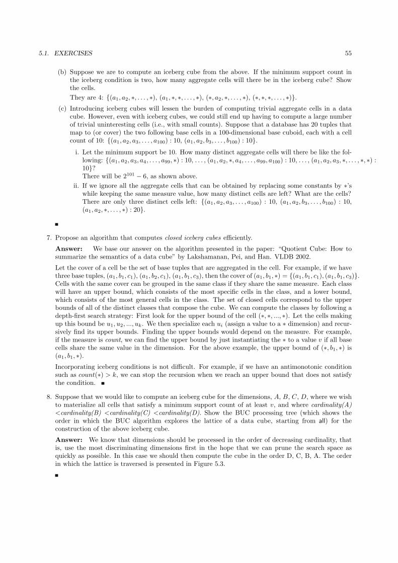
5.1. EXERCISES 55
(b) Suppose we are to compute an iceberg cube from the above. If the minimum support count inthe iceberg condition is two, how many aggregate cells will there be in the iceberg cube? Showthe cells.
They are 4: {(a1, a2, ∗, . . . , ∗), (a1, ∗, ∗, . . . , ∗), (∗, a2, ∗, . . . , ∗), (∗, ∗, ∗, . . . , ∗)}.(c) Introducing iceberg cubes will lessen the burden of computing trivial aggregate cells in a data
cube. However, even with iceberg cubes, we could still end up having to compute a large numberof trivial uninteresting cells (i.e., with small counts). Suppose that a database has 20 tuples thatmap to (or cover) the two following base cells in a 100-dimensional base cuboid, each with a cellcount of 10: {(a1, a2, a3, . . . , a100) : 10, (a1, a2, b3, . . . , b100) : 10}.
i. Let the minimum support be 10. How many distinct aggregate cells will there be like the fol-lowing: {(a1, a2, a3, a4, . . . , a99, ∗) : 10, . . . , (a1, a2, ∗, a4, . . . , a99, a100) : 10, . . . , (a1, a2, a3, ∗, . . . , ∗, ∗) :10}?There will be 2101 − 6, as shown above.
ii. If we ignore all the aggregate cells that can be obtained by replacing some constants by ∗’swhile keeping the same measure value, how many distinct cells are left? What are the cells?There are only three distinct cells left: {(a1, a2, a3, . . . , a100) : 10, (a1, a2, b3, . . . , b100) : 10,(a1, a2, ∗, . . . , ∗) : 20}.
7. Propose an algorithm that computes closed iceberg cubes efficiently.
Answer: We base our answer on the algorithm presented in the paper: “Quotient Cube: How tosummarize the semantics of a data cube” by Lakshamanan, Pei, and Han. VLDB 2002.
Let the cover of a cell be the set of base tuples that are aggregated in the cell. For example, if we havethree base tuples, (a1, b1, c1), (a1, b2, c1), (a1, b1, c3), then the cover of (a1, b1, ∗) = {(a1, b1, c1), (a1, b1, c3)}.Cells with the same cover can be grouped in the same class if they share the same measure. Each classwill have an upper bound, which consists of the most specific cells in the class, and a lower bound,which consists of the most general cells in the class. The set of closed cells correspond to the upperbounds of all of the distinct classes that compose the cube. We can compute the classes by following adepth-first search strategy: First look for the upper bound of the cell (∗, ∗, ..., ∗). Let the cells makingup this bound be u1, u2, ..., uk. We then specialize each ui (assign a value to a ∗ dimension) and recur-sively find its upper bounds. Finding the upper bounds would depend on the measure. For example,if the measure is count, we can find the upper bound by just instantiating the ∗ to a value v if all basecells share the same value in the dimension. For the above example, the upper bound of (∗, b1, ∗) is(a1, b1, ∗).Incorporating iceberg conditions is not difficult. For example, if we have an antimonotonic conditionsuch as count(∗) > k, we can stop the recursion when we reach an upper bound that does not satisfythe condition.
8. Suppose that we would like to compute an iceberg cube for the dimensions, A, B, C, D, where we wishto materialize all cells that satisfy a minimum support count of at least v, and where cardinality(A)<cardinality(B) <cardinality(C) <cardinality(D). Show the BUC processing tree (which shows theorder in which the BUC algorithm explores the lattice of a data cube, starting from all) for theconstruction of the above iceberg cube.
Answer: We know that dimensions should be processed in the order of decreasing cardinality, thatis, use the most discriminating dimensions first in the hope that we can prune the search space asquickly as possible. In this case we should then compute the cube in the order D, C, B, A. The orderin which the lattice is traversed is presented in Figure 5.3.

56 CHAPTER 5. DATA CUBE TECHNOLOGY
2 D
1 all
10 C 14 B 16 A
3 DC
4 DCB
5 DCBA
7 DB
6 DCA
9 DA 11 CB 13 CA 15 BA
8 DBA 12 CBA
Figure 5.3: BUC processing order for Exercise 5.8.
9. Discuss how you might extend the Star-Cubing algorithm to compute iceberg cubes where the icebergcondition tests for an avg that is no bigger than some value, v.
Answer:
Instead of using average we can use the bottom-k average of each cell, which is antimonotonic. If thebottom-k average of a cell is larger than v, we can be sure than no descendant cell (a cell with less *dimensions) can have a bottom-k average smaller than v.
To reduce the amount of space required to check the bottom-k average condition, we can store a fewstatistics such as count and sum for the base tuples that fall between a certain range of v (e.g., lessthan v, [1.0-1.2) times v, [1.2-1.4) times v, etc.) and use these few values for pruning.
10. A flight data warehouse for a travel agent consists of six dimensions: traveler, departure (city), de-parture time, arrival, arrival time, and flight; and two measures: count, and avg fare, where avg farestores the concrete fare at the lowest level but average fare at other levels.
(a) Suppose the cube is fully materialized. Starting with the base cuboid [traveler, departure, de-parture time, arrival, arrival time, flight ], what specific OLAP operations (e.g., roll-up flight toairline) should one perform in order to list the average fare per month for each business travelerwho flies American Airlines (AA) from L.A. in the year 2009?
(b) Suppose we want to compute a data cube where the condition is that the minimum number ofrecords is 10 and the average fare is over $500. Outline an efficient cube computation method(based on common sense about flight data distribution).
Answer:
(a) Suppose the cube is fully materialized. Starting with the base cuboid [traveller, departure,departure time, arrival, arrival time, flight], what specific OLAP operations (e.g., roll-upflight to airline) should one perform in order to list the average fare per month for each businesstraveler who flies American Airlines (AA) from L.A. in the year 2009?
The OLAP operations are:
i. roll-up on traveler to the level of category and dice on “business”
ii. roll-up on departure to the level of city and dice on “L.A.”

5.1. EXERCISES 57
iii. roll-up on departure time to the level of year and dice on “2009”
iv. roll-up on arrival to the level of “ANY” (∗)v. roll-up on arrival time to the level of “ANY” (∗)vi. roll-up on flight to the level of company and dice on “AA”
vii. drill-down on traveler to the level of individual
viii. drill-down on departure time to the level of month.
(b) Suppose we want to compute a data cube where the condition is that the minimum number ofrecords is 10 and the average fare is over $500. Outline an efficient cube computation method(based on common sense about flight data distribution).
There are two constraints: min sup = 10 and avg fare > 500. Use an iceberg cubing algorithm,such as BUC. Since avg fare > 500 is not antimonotonic, it should be converted into a top-k-avg,i.e., avg10(fare) > 500. Use binning plus min sup to prune the computation of the cube.
11. (Implementation project) There are four typical data cube computation methods: MultiWay[ZDN97], BUC [BR99], H-cubing [HPDW01], and Star-cubing [XHLW03].
(a) Implement any one of these cube computation algorithms and describe your implementation,experimentation, and performance. Find another student who has implemented a different algo-rithm on the same platform (e.g., C++ on Linux) and compare your algorithm performance withhis/hers.
Input:
i. An n-dimensional base cuboid table (for n < 20), which is essentially a relational table withn attributes
ii. An iceberg condition: count (C) ≥ k where k is a positive integer as a parameter
Output:
i. The set of computed cuboids that satisfy the iceberg condition, in the order of your outputgeneration
ii. Summary of the set of cuboids in the form of “cuboid ID : the number of nonempty cells”,sorted in alphabetical order of cuboids, e.g., A:155, AB : 120, ABC : 22, ABCD : 4, ABCE : 6,ABD : 36, where the number after “:” represents the number of nonempty cells. (This is usedto quickly check the correctness of your results.)
(b) Based on your implementation, discuss the following:
i. What challenging computation problems are encountered as the number of dimensions growslarge?
ii. How can iceberg cubing solve the problems of part (a) for some data sets (and characterizesuch data sets)?
iii. Give one simple example to show that sometimes iceberg cubes cannot provide a good solution.
(c) Instead of computing a data cube of high dimensionality, we may choose to materialize the cuboidsthat have only a small number of dimension combinations. For example, for a 30-dimensionaldata cube, we may only compute the 5-dimensional cuboids for every possible 5-dimensionalcombination. The resulting cuboids form a shell cube. Discuss how easy or hard it is to modifyyour cube computation algorithm to facilitate such computation.
Answer:
(a) There is no standard answer for an implementation project. This is to be evaluated on an indi-vidual basis.
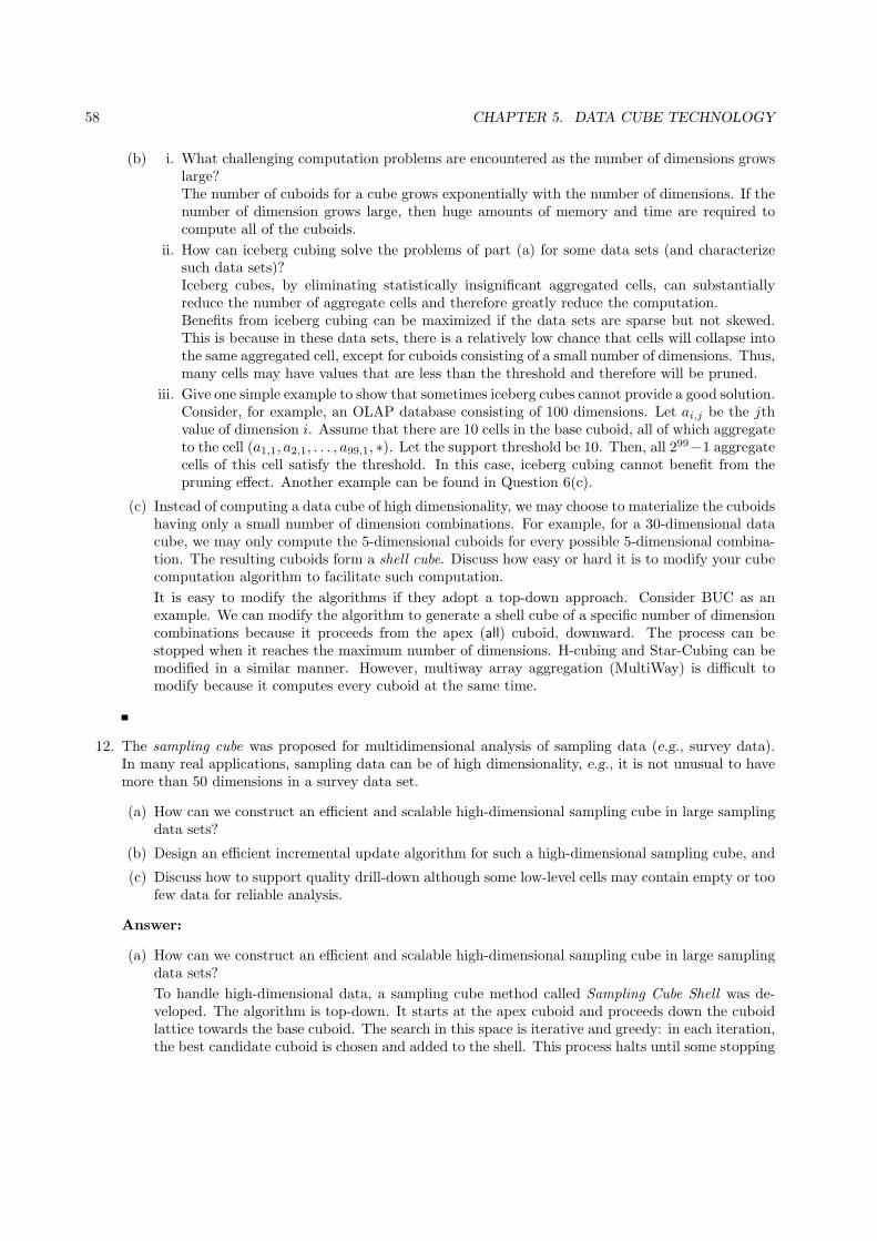
58 CHAPTER 5. DATA CUBE TECHNOLOGY
(b) i. What challenging computation problems are encountered as the number of dimensions growslarge?The number of cuboids for a cube grows exponentially with the number of dimensions. If thenumber of dimension grows large, then huge amounts of memory and time are required tocompute all of the cuboids.
ii. How can iceberg cubing solve the problems of part (a) for some data sets (and characterizesuch data sets)?Iceberg cubes, by eliminating statistically insignificant aggregated cells, can substantiallyreduce the number of aggregate cells and therefore greatly reduce the computation.Benefits from iceberg cubing can be maximized if the data sets are sparse but not skewed.This is because in these data sets, there is a relatively low chance that cells will collapse intothe same aggregated cell, except for cuboids consisting of a small number of dimensions. Thus,many cells may have values that are less than the threshold and therefore will be pruned.
iii. Give one simple example to show that sometimes iceberg cubes cannot provide a good solution.Consider, for example, an OLAP database consisting of 100 dimensions. Let ai,j be the jthvalue of dimension i. Assume that there are 10 cells in the base cuboid, all of which aggregateto the cell (a1,1, a2,1, . . . , a99,1, ∗). Let the support threshold be 10. Then, all 299−1 aggregatecells of this cell satisfy the threshold. In this case, iceberg cubing cannot benefit from thepruning effect. Another example can be found in Question 6(c).
(c) Instead of computing a data cube of high dimensionality, we may choose to materialize the cuboidshaving only a small number of dimension combinations. For example, for a 30-dimensional datacube, we may only compute the 5-dimensional cuboids for every possible 5-dimensional combina-tion. The resulting cuboids form a shell cube. Discuss how easy or hard it is to modify your cubecomputation algorithm to facilitate such computation.
It is easy to modify the algorithms if they adopt a top-down approach. Consider BUC as anexample. We can modify the algorithm to generate a shell cube of a specific number of dimensioncombinations because it proceeds from the apex (all) cuboid, downward. The process can bestopped when it reaches the maximum number of dimensions. H-cubing and Star-Cubing can bemodified in a similar manner. However, multiway array aggregation (MultiWay) is difficult tomodify because it computes every cuboid at the same time.
12. The sampling cube was proposed for multidimensional analysis of sampling data (e.g., survey data).In many real applications, sampling data can be of high dimensionality, e.g., it is not unusual to havemore than 50 dimensions in a survey data set.
(a) How can we construct an efficient and scalable high-dimensional sampling cube in large samplingdata sets?
(b) Design an efficient incremental update algorithm for such a high-dimensional sampling cube, and
(c) Discuss how to support quality drill-down although some low-level cells may contain empty or toofew data for reliable analysis.
Answer:
(a) How can we construct an efficient and scalable high-dimensional sampling cube in large samplingdata sets?
To handle high-dimensional data, a sampling cube method called Sampling Cube Shell was de-veloped. The algorithm is top-down. It starts at the apex cuboid and proceeds down the cuboidlattice towards the base cuboid. The search in this space is iterative and greedy: in each iteration,the best candidate cuboid is chosen and added to the shell. This process halts until some stopping

5.1. EXERCISES 59
condition is met. The condition could be a space constraint, e.g., the number of cuboids builtcannot exceed some value. Or it could be an information constraint, e.g., the gain in building anew cuboid must exceed some minimum.
Specifically speaking, initially, only the all or apex cuboid exists. By definition, it contains exactlyone cell and the standard deviation of it is the standard deviation of all the samples put together.The child cuboids of the apex cuboid are then added into a candidate set. The best cuboid iscomputed. In the paper, the measure is the reduction in the amount of variance with respect tothe cube value in its cells from one of the cuboid’s parents. Then this candidate cuboid is chosenand added to the shell. Its children in the cuboid lattice are added to the candidate set. Thisprocess iterates until a stopping criterion is met. Note that the final data structure is not strictlya tree since a node could have multiple parents. It is just a portion (i.e., shell) of the completedata cube lattice.
(b) Design an efficient incremental update algorithm for such a high-dimensional sampling cube.
In order to handle incremental data updates for such a high-dimensional sampling cube, theSampling Cube Shell is first recomputed as described in (a). Then we simply compute newcuboids in the shell fragments and update the existing shell fragments. The ID table should beupdated accordingly. The update is efficient since all the mean and confidence interval measuresof the data cube are algebraic. Note that our cube is build top-down, so the cells in the high-levelcuboids often contain quite many samples.
(c) Discuss how to support quality drill-down although some low-level cells may contain empty or toofew data for reliable analysis.
The best way to solve this small sample size problem is to simply get more data. There are twopossible methods to expand the query and get more data to boost the confidence. They bothexpand the original query in the data cube, just in different directions.
The first one is Intra-Cuboid Query Expansion. In the intra-cuboid case, the expansion occurs bylooking at nearby cells in the same cuboid as the queried cell. Dimensions which are uncorrelatedor weakly correlated with the measure value (i.e., the value to be predicted) are the best candidatesfor expansion. Next we should select semantically similar values within those dimension(s) tominimize the risk of altering the final result.
The second is Inter-Cuboid Query Expansion. Here the expansion occurs by looking to a moregeneral cell. And the strategy is similar: correlated dimensions are not allowed in inter-cuboidexpansions.
Some references for the answer to this question:
[1] Xiaolei Li, Jiawei Han, Zhijun Yin, Jae-Gil Lee, and Yizhou Sun, ”Sampling Cube: A Frameworkfor Statistical OLAP over Sampling Data”, Proc. 2008 ACM SIGMOD Int. Conf. on Management ofData (SIGMOD’08), Vancouver, BC, Canada, June 2008.
13. The ranking cube was proposed for efficient computation of top-k (ranking) queries in relationaldatabases. Recently, researchers have proposed another kind of queries, called skyline queries. Askyline query returns all the objects pi such that pi is not dominated by any other object pj , wheredominance is defined as follows. Let the value of pi on dimension d be v(pi, d). We say pi is dominatedby pj if and only if for each preference dimension d, v(pj , d) ≤ v(pi, d), and there is at least one dwhere the equality does not hold.
(a) Design a ranking cube so that skyline queries can be processed efficiently.
(b) Skyline queries are sometimes too strict to be desirable to some users. One may generalize theconcept of skyline into generalized skyline as below: Given a d-dimensional database and a queryq, the generalized skyline is the set of the following objects: (1) the skyline objects, and (2) thenon-skyline objects that are ϵ-neighbors of a skyline object, where r is an ϵ-neighbor of an object

60 CHAPTER 5. DATA CUBE TECHNOLOGY
p if the distance between p and r is no more than ϵ. Design a ranking cube to process generalizedskyline queries efficiently.
Answer:
(a) Design a ranking cube so that skyline queries can be processed efficiently.
In order to design a ranking cube so that skyline queries can be processed efficiently, one datapartition P over the preference dimensions (e.g., price and mileage) need to be created. Using Pas the template, one can summarize the data distribution over P for each cell by indicating whichregions in the partition contain data belonging to the cell. For instance, P may partition datainto n regions r1, r2, ..., rn. A cell (e.g., type = sedan) corresponds to a subset of data, which mayonly appear in m ≤ n regions r′1, · · · , r′m. A data summarization remembers those m regions.Comparing with a completely new data partition, the data summarization is much cheaper inboth computational and storage cost. The data summarization is a bridge to join the booleanselection condition and preference search during online query processing. More specifically, thequery algorithm progressively visits (in P ) a sequence of regions that are promising for userpreference (e.g., rq1, · · · , r
qj ), but skips those regions rqi which do not satisfy boolean selections
rqi /∈ {r′1, · · · , r′m}). By doing this, the query processing pushes both boolean and preferencepruning deep into the search.
The prune procedure has two main tasks: domination pruning and boolean pruning. The dom-ination pruning for skylines are straightforward: simply comparing the value in each dimensionbetween the submitted entry e (i.e., data objects or regions mentioned above) and the previouslydiscovered skylines. If e is dominated by any of them, e can be pruned. The boolean pruningis accomplished by signatures (the data summarization mentioned above), checking whether theentry e submitted to the prune procedure should be skipped or not.
Specifically, every region n is associated with a value d(n) used for comparison, where d(n) =
minx∈n(∑j
i=1 N′i(x)) is the lower bound value over the region covered by n, and N ′
i(x) is thevalue of object x on preference dimension N ′
i . Clearly, a data object t cannot be dominated by
any data objects contained by region n if∑j
i=1 N′i(t) ≤ d(n). On the other hand, if a region n is
dominated by some data object t, all child regions of n are dominated by t. By the way, everyentry e comes from a heap with minimal d(e).
The signature-based query processing is listed in the Figure 5.4.
One can easily verify the correctness of the algorithm for skyline queries. The results are generatedon Line 8, and all data objects e on Line 8 are valid skylines. This is true because: (1) e passesthe boolean pruning, and thus e satisfies the boolean predicate; and (2) e passes the preferencepruning, and thus e is not dominated by previous skylines.
(b) Skyline queries are sometimes too strict to be desirable to some users. One may generalize theconcept of skyline into generalized skyline as below: Given a d-dimensional database and a queryq, the generalized skyline is the set of the following objects: (1) the skyline objects, and (2) thenon-skyline objects that are ϵ-neighbors of a skyline object, where r is an ϵ-neighbor of an objectp if the distance between p and r is no more than ϵ. Design a ranking cube to process generalizedskyline queries efficiently.
The cube which processes generalized skyline queries is similar to the one described in the question(a). We first adopt algorithm in question (a) to obtain the top-k skyline queries. To get thoseϵ-neighbors, the domination pruning part for skylines in the algorithm should be modified for thepurpose of pruning for ϵ-neighbors. That is, we run the algorithm again but compare the value ineach dimension between the submitted entry e and the previously obtained top-k skyline queriesinstead.
Some references for the answer to this question: [1] Dong Xin and Jiawei Han, “P-Cube: AnsweringPreference Queries in multiDimensional Space”, Proc. 2008 Int. Conf. on Data Engineering (ICDE’08),

5.1. EXERCISES 61
Figure 5.4: signature-based query processing of Exercise 5.13.
Cancun, Mexico, April 2008.
14. The ranking cube was designed to support top-k (ranking) queries in relational database systems.However, ranking queries are also posed to data warehouses, where ranking is on multidimensionalaggregates instead of on measures of base facts. For example, consider a product manager who isanalyzing a sales database that stores the nationwide sales history, organized by location and time. Inorder to make investment decisions, the manager may pose the following queries: “What are the top-10(state, year) cells having the largest total product sales?” and he may further drill-down and ask, “Whatare the top-10 (city, month) cells?” Suppose the system can perform such partial materialization toderive two types of materialized cuboids: a guiding cuboid and a supporting cuboid, where the formercontains a number of guiding cells that provide concise, high-level data statistics to guide the rankingquery processing, whereas the latter provides inverted indices for efficient online aggregation.
(a) Derive an efficient method for computing such aggregate ranking cubes.
(b) Extend your framework to handle more advanced measures. One such example could be as follows.Consider an organization donation database, where donors are grouped by “age”, “income”, andother attributes. Interesting questions include: “Which age and income groups have made thetop-k average amount of donation (per-donor)?” and “Which income group of donors has thelargest standard deviation in the donation amount?”
Answer:
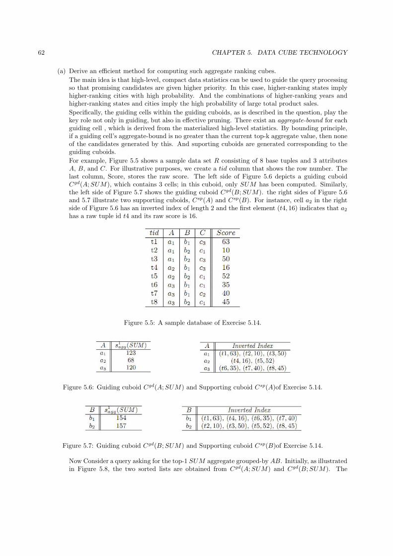
62 CHAPTER 5. DATA CUBE TECHNOLOGY
(a) Derive an efficient method for computing such aggregate ranking cubes.
The main idea is that high-level, compact data statistics can be used to guide the query processingso that promising candidates are given higher priority. In this case, higher-ranking states implyhigher-ranking cities with high probability. And the combinations of higher-ranking years andhigher-ranking states and cities imply the high probability of large total product sales.
Specifically, the guiding cells within the guiding cuboids, as is described in the question, play thekey role not only in guiding, but also in effective pruning. There exist an aggregate-bound for eachguiding cell , which is derived from the materialized high-level statistics. By bounding principle,if a guiding cell’s aggregate-bound is no greater than the current top-k aggregate value, then noneof the candidates generated by this. And suporting cuboids are generated corresponding to theguiding cuboids.
For example, Figure 5.5 shows a sample data set R consisting of 8 base tuples and 3 attributesA, B, and C. For illustrative purposes, we create a tid column that shows the row number. Thelast column, Score, stores the raw score. The left side of Figure 5.6 depicts a guiding cuboidCgd(A;SUM), which contains 3 cells; in this cuboid, only SUM has been computed. Similarly,the left side of Figure 5.7 shows the guiding cuboid Cgd(B;SUM). the right sides of Figure 5.6and 5.7 illustrate two supporting cuboids, Csp(A) and Csp(B). For instance, cell a2 in the rightside of Figure 5.6 has an inverted index of length 2 and the first element (t4, 16) indicates that a2has a raw tuple id t4 and its raw score is 16.
Figure 5.5: A sample database of Exercise 5.14.
Figure 5.6: Guiding cuboid Cgd(A;SUM) and Supporting cuboid Csp(A)of Exercise 5.14.
Figure 5.7: Guiding cuboid Cgd(B;SUM) and Supporting cuboid Csp(B)of Exercise 5.14.
Now Consider a query asking for the top-1 SUM aggregate grouped-by AB. Initially, as illustratedin Figure 5.8, the two sorted lists are obtained from Cgd(A;SUM) and Cgd(B;SUM). The

5.1. EXERCISES 63
aggregate-bound of each guiding cell is initialized to be the materialized SUM and the guidingcells in each list are sorted descendingly according to the aggregate-bound. Next, we pull outthe top guiding cell from each list and combine them to generate the first candidate cell, (a1, b2).The intuition is straightforward as a1 and b2 have larger SUM than any other cell does. It is,however, not possible to terminate early until we verify its true aggregate value and make sureany unseen candidate cell has no greater aggregate. To verify the true aggregate, we turn to theinverted indices of a1 and b2 in Csp(A) and Csp(B), respectively. We retrieve their indices andintersect the two tid-lists, which results in {t2, t3}, and then compute the SUM of the raw scoresover the intersecting tid-list, which results in FQ
agg(a1, b2) = 10 + 50 = 60.
Having known that SUM(a1, b2) = 60, we can infer that∑
j =2 SUM(a1, bj) = SUM(a1) −SUM(a1, b2) = 123 − 60 = 63. This means that any unseen cell (a1, bj)(j = 2) must satisfySUM(a1, bj) ≤ 63. Thus, we update the aggregate-bound F agg(a1) from 123 to 63 (Figure 5.9).For the same reason, F agg(b2) can be updated from 157 to 97, implying that SUM(ai, b2) ≤97(i = 1) .
Here, The aggregate-bound of a guiding cell g, F agg(g), is the maximum possible aggregate (FQagg)
of any unseen candidate cell that could be combined by g.
After the first candidate verification, as shown in Figure 5.9, the order of the guiding cells in thetwo sorted lists has changed due to the update. The top-1 cell from the two lists are now a3 andb1, respectively. We generate the sec ond candidate (a3, b1) in the same fashion. To verify it, weintersect the tid’s of a3 and b1, which results in {t6, t7} and SUM(a3, b1) = 35 + 40 = 75. Then,we update F agg(a3) to 120− 75 = 45 and F agg(b1) to 154− 75 = 79 and adjust the sorted lists,as shown in Figure 5.10. At the time, the maximum aggregate-bound in the sorted list for ai,F agg(a2) = 68, is no greater than the current top-1 aggregate value, 75. Although both F agg(b1)are F agg(b2) are still greater than 75, it is impossible to find any ai such that FQ
agg(ai, bj) couldbe greater than 75. Therefore, we can terminate the query process and output (a3, b1) : 75 as thefinal top-1.
Figure 5.8: Initial sorted lists of Exercise 5.14.
Figure 5.9: Sorted lists after the first candidate verification of Exercise 5.14.
Similarly, the strategy described above can be easily extended to the top-k situation. And thisquery execution algorithm for the top-k cells QueryExec() is give in Figure 5.11 .
(b) Extend your framework to handle more advanced measures. One such example could be as follows.Consider an organization donation database, where donors are grouped by “age”, “income”, andother attributes. Interesting questions include: “Which age and income groups have made the

64 CHAPTER 5. DATA CUBE TECHNOLOGY
Figure 5.10: Sorted lists after the second candidate verification of Exercise 5.14.
top-k average amount of donation (per-donor)?” and “Which income group of donors has thelargest standard deviation in the donation amount?”
To handle more general types of query measures, we extend QueryExec(). While the candidategeneration and verification framework remains unchanged, their key difference lies in the com-putation of the aggregate-bound F agg(g) for any guiding cell g. By bounding principle, F agg(g)should represent the maximum possible aggregate value of any candidate c generated by g, i.e.,F agg(g) ≥ FQ
agg(c) must always hold for the query measure FQagg. Therefore, the aggregate-bound
for SUM cannot work for other query measures. We address the problem of aggregate-boundcomputation for different measures in two aspects: (1) the initialization F agg(g) for all guidingcells; and (2) how to update F agg(g).
Figure 5.12 lists the guiding measures and the initial aggregate- bound for different query mea-sures. To initialize the aggregate-bound of guiding cells for a particular query measure F agg, itscorresponding guiding measuresM should be already materialized. The initialization process issimilar to QueryExec() in that N sorted lists are created, each containing all the guiding cells inthe corresponding guiding cuboid. For each guiding cell, its materialized guiding measure valuesare retrieved, and its aggregate-bound is computed using Γ on the materialized measure values.
Updating the aggregate-bound is equally important as the initialization because the aggregate-bound is monotonically decreasing, providing an increasingly tighter bound to prune more guidingcells. Starting from the measures in Figure 5.12, we can see that any FQ
agg in the table can bederived from one or two of the four guiding measures, SUM , COUNT , MAX, and MIN . ForSUM , as we have discussed, the updating procedure is F agg(g) ← F agg(g) − FQ
agg(c), where ga guiding cell and c is a candidate generated by g. This procedure applies to COUNT as well.For MAX and MIN , the updating procedure is as follows. We maintain the set of g’s rawscores, denoted as Sg, during the fetching process. After the intersection of the inverted indicesof all guiding cells, we can also know the set of c’s raw scores, denoted as Sc(⊆ Sg). Thus, theupdated MAX(g) would be max(Sg−Sc), whereas the updated MIN(g) would be min(Sg−Sc).Finally, after all the updated guiding measure values are obtained, Γ can be applied to calculatethe updated aggregate-bound F agg(g), which must be monotonically decreasing.
Some references for the answer to this question:
[1] Tianyi Wu, Dong Xin, and Jiawei Han, “ARCube: Supporting Ranking Aggregate Queries inPartially Materialized Data Cubes”, Proc. 2008 ACM SIGMOD Int. Conf. on Management of Data(SIGMOD’08), Vancouver, BC, Canada, June 2008.
15. The prediction cube is a good example of multidimensional data mining in cube space.
(a) Propose an efficient algorithm that computes prediction cubes in a given multidimensional database;and
(b) For what kind of classification models can your algorithm be applied. Explain.
Answer:

5.1. EXERCISES 65
Figure 5.11: Query execution algorithm for SUM of Exercise 5.14.
(a) Propose an efficient algorithm that computes prediction cubes in a given multidimensional database.
A naıve way to fully materialize a prediction cube is to exhaustively build models and evaluatethem for each cell and for each granularity. This method is very expensive if the base data setis large. An ensemble method called Probability-Based Ensemble (PBE) was developedas a more feasible alternative. It requires model construction for only the finest-grained cells.OLAP-style bottom-up aggregation is then used to generate the values of the coarser-grainedcells.
Let the finest-grained subsets (i.e., finest-grained cells) be called the base subsets, denoted bybi(D), for i = 1, . . . , B, where B is the product of the sizes of the least general domains. Then everycube subset can be represented as the union of some base subsets of D, i.e., σS(D) = ∪i∈Sbi(D),where S ⊆ {1, . . . , B} denotes a cube subset.
The prediction of a predictive model can be seen as finding a class label that maximizes a scoringfunction. Formally, consider a predictive model h(X;σS(D)) trained on subset σS(D) usingfeatures X to predict the class label. The prediction of h(X;σS(D)) on input tuple x can bemodeled as maximizing a scoring function Score(y|x;σS(D)); i.e.,
h(x|σS(D)) = argmaxyScore(y|x, σSD).
The prediction of a predictive model can be seen as finding a class label that maximizes a scoringfunction. PBE was developed to approximately make the scoring function of any predictive modeldistributively decomposable.

66 CHAPTER 5. DATA CUBE TECHNOLOGY
Figure 5.12: Aggregate measures and their corresponding guiding measures and aggregate-bound of Exercise5.14.
(b) For what kind of classification models can your algorithm be applied. Explain.
If the scoring function used is distributively or algebraically decomposable, prediction cubes canalso be computed with efficiency. Previous studies have shown that the naıve Bayes classifier hasan algebraically decomposable scoring function, and the kernel density-based classifier has a dis-tributively decomposable scoring function. Therefore, either of these could be used to implementprediction cubes efficiently. The PBE method presents a novel approach to multidimensional datamining in cube space.
16. Multifeature cubes allow us to construct interesting data cubes based on rather sophisticated queryconditions. Can you construct the following multifeature cube by translating the following user requestsinto queries using the form introduced in this textbook?
(a) Construct smart shopper cube where a shopper is smart if at least 10% of the goods she buys ineach shopping are on sale; and
(b) Construct a datacube for best-deal products where best-deal products are those products whoseprice is the lowest for this product in the given month.
Answer: There exist problems in this question.
The “such that” phrase in the multifeature cube is not able to filter not smart shoppers, and is onlyable to find the cells satisfying some conditions. On the other hand, the “where” phrase is designedto be able to do the filtering. In order to build the cubes with smart shoppers, I think we first needto remove those not smart shoppers. But if we use “where” to filter shoppers, the motivation of usingmultifeature cube is not clear.
In the example of the textbook, the multifeature cube does operations around the measure “price”,which is easier to deal with since it is not like what we need to do in the question 16 where a shopper issmart or not. In other words, the feature “is smart” is more correlated with “shopper” which cannotbe aggregated easily, while “price” can be efficiently aggregated according to different dimensions likeregion or time (i.e. in cuboid region time, the “is smart” measure does not make sense).
The “best-deal product” is similar to certain extent.
17. Discovery-driven cube exploration is a desirable way to mark interesting points among a large number ofcells in a data cube. Individual users may have different views on whether a point should be consideredinteresting enough to be marked. Suppose one would like to mark those objects whose absolute valueof Z score is over 2 in every row and column in a d-dimensional plane.
(a) Derive an efficient computation method to identify such points during the data cube computation.
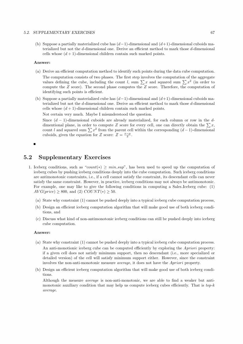
5.2. SUPPLEMENTARY EXERCISES 67
(b) Suppose a partially materialized cube has (d−1)-dimensional and (d+1)-dimensional cuboids ma-terialized but not the d-dimensional one. Derive an efficient method to mark those d-dimensionalcells whose (d+ 1)-dimensional children contain such marked points.
Answer:
(a) Derive an efficient computation method to identify such points during the data cube computation.
The computation consists of two phases. The first step involves the computation of the aggregatevalues defining the cube, including the count l, sum
∑x and squared sum
∑x2 (in order to
compute the Z score). The second phase computes the Z score. Therefore, the computation ofidentifying such points is efficient.
(b) Suppose a partially materialized cube has (d−1)-dimensional and (d+1)-dimensional cuboids ma-terialized but not the d-dimensional one. Derive an efficient method to mark those d-dimensionalcells whose (d+ 1)-dimensional children contain such marked points.
Not certain very much. Maybe I misunderstood the question.
Since (d − 1)-dimensional cuboids are already materialized, for each column or row in the d-dimentional plane, in order to compute Z score for every cell, one can directly obtain the
∑x,
count l and squared sum∑
x2 from the parent cell within the corresponding (d− 1)-dimensionalcuboids, given the equation for Z score: Z = x−µ
δ .
5.2 Supplementary Exercises
1. Iceberg conditions, such as “count(∗) ≥ min sup”, has been used to speed up the computation oficeberg cubes by pushing iceberg conditions deeply into the cube computation. Such iceberg conditionsare antimonotonic constraints, i.e., if a cell cannot satisfy the constraint, its descendant cells can neversatisfy the same constraint. However, in practice, iceberg conditions may not always be antimonotonic.For example, one may like to give the following conditions in computing a Sales Iceberg cube: (1)AV G(price) ≥ 800, and (2) COUNT (∗) ≥ 50.
(a) State why constraint (1) cannot be pushed deeply into a typical iceberg cube computation process,
(b) Design an efficient iceberg computation algorithm that will make good use of both iceberg condi-tions, and
(c) Discuss what kind of non-antimonotonic iceberg conditions can still be pushed deeply into icebergcube computation.
Answer:
(a) State why constraint (1) cannot be pushed deeply into a typical iceberg cube computation process.
An anti-monotionic iceberg cube can be computed efficiently by exploring the Apriori property:if a given cell does not satisfy minimum support, then no descendant (i.e., more specialized ordetailed version) of the cell will satisfy minimum support either. However, since the constraintinvolves the non-anti-monotonic measure average, it does not have the Apriori property.
(b) Design an efficient iceberg computation algorithm that will make good use of both iceberg condi-tions.
Although the measure average is non-anti-monotonic, we are able to find a weaker but anti-monotonic auxiliary condition that may help us compute iceberg cubes efficiently. That is top-kaverage.

68 CHAPTER 5. DATA CUBE TECHNOLOGY
A cell c is said to have n base cells if it covers n nonempty descendant base cells. The top-kaverage of c, denoted as avgk(c), is the average value of the top-k base cells of c (i.e., the first kcells when all the base cells in c are sorted in value-descending order) if k ≤ n; or −∞ if k > n.
Then we have the Top-k Apriori : Let c be a cell which fails to satisfy avgk(c) ≥ v in cube B(AvgI).If a cell c′ is a descendant of c, then c′ cannot satisfy avgk(c′) ≥ v in cube B(Sales Iceberg).Here v is the value in the constraint (800 in this quesition) and B(Sales Iceberg) is called thebackground cube which is the cube without the iceberg condition.
Even we get the above top-k apriori property, to keep tracking of top k values for each cell in anm-dimensional space seems to be a nontrivial cost. Therefore, a binning technique is proposedwhich can be used to reduce the cost of storage and computation of top-k average.
For example, suppose v ≥ 0, one can set up the range of five bins as follows: range(bin[1]) =[v,∞), range(bin[2]) = [0.95v, v), range(bin[3]) = [0.85v, 0.95v), range(bin[4]) = [0.70v, 0.85v),and range(bin[5]) = [0.50v, 0.70v). Notice since we have count and sum of all the cells, that forthe remaining range [−∞, 0.50v) can be derived easily.
The set of bins for a cell c can be used to judge wheter avgk(c) ≥ v is false as follows. Let mbe the smallest number such that the sum of counts of the upper m bins is no less than k, i.e.,countm =
∑mi=1 count(bini) ≥ k. We approximate avgk(c) using:
avg′k(c) = (m−1∑i=1
sum(bini) +max(binm)× nk)/k
where nk = k −∑m−1
i=1 count(bini).
Note that avgk(c) ≤ avg′k(c). Consequenty, if avg′k(c) < v, then do descendant of c can satisfythe constraint in Sales iceberg.
Based on the above discussion, one can easily extend the BUC iceberg cube computation algorithmto compute iceberg cubes with average.
(c) Discuss what kind of non-antimonotonic iceberg conditions can still be pushed deeply into icebergcube computation.
• Compute iceberg cube whose AVG is no bigger than a value.
• Compute iceberg cubes with AVG constraint only.
• Compute iceberg cubes whose measure is SUM of positive and negative values.
• Compute iceberg cubes with measures like max, min, count, and p sum, where p sum meansthe sum of all nonnegative base cell values in a cube.
• Compute iceberg cubes having conjunctions of multiple conditions with different measures.
Some references for the answer to this question:
[1] J. Han, J. Pei, G. Dong, K. Wang. Efficient Computation of Iceberg Cubes With Complex Measures.SIGMOD01

Chapter 6
Mining Frequent Patterns,Associations, and Correlations: BasicConcepts and Methods
6.1 Exercises
1. Suppose you have the set C of all frequent closed itemsets on a data set D, as well as the supportcount for each frequent closed itemset. Describe an algorithm to determine whether a given itemset Xis frequent or not, and the support of X if it is frequent.
Answer:
Algorithm: Itemset Freq Tester. Determine if an itemset is frequent.
Input: C, set of all frequent closed itemsets along with their support counts; test itemset, X.
Output: Support of X if it is frequent, otherwise -1.
Method:
(1) s = ∅;(2) for each itemset, l ∈ C(3) if X ⊂ l and (length(l) < length(s) or s = ∅) then {(4) s = l;(5) }(6) if s = ∅ then {(7) return support(s);(8) }(9) return -1;
2. An itemset X is called a generator on a data set D if there does not exist a proper sub-itemset Y ⊂ Xsuch that support(X) = support(Y ). A generator X is a frequent generator if support(X) passes theminimum support threshold. Let G be the set of all frequent generators on a data set D.
(a) Can you determine whether an itemset A is frequent and the support of A, if it is frequent,using only G and the support counts of all frequent generators? If yes, present your algorithm.
69

70CHAPTER 6. MINING FREQUENT PATTERNS, ASSOCIATIONS, AND CORRELATIONS: BASIC CONCEPTS ANDMETHODS
Otherwise, what other information is needed? Can you give an algorithm assuming the informationneeded is available?
(b) What is the relationship between closed itemsets and generators?
Answer:
(a) Can you determine whether an itemset A is frequent and the support of A, if it is frequent,using only G and the support counts of all frequent generators? If yes, present your algorithm.Otherwise, what other information is needed? Can you give an algorithm assuming the informationneeded is available?
No, the frequent generators alone do not provide enough information to represent the complete setof frequent itemsets. We need information such as the ”positive border” of the frequent generators,that is, all itemsets l such that l is frequent, l is not a frequent generator, and all proper subsetsof l are frequent generators. With this information we may use the following algorithm:
Algorithm: InferSupport. Determine if an itemset is frequent.
Input:
• l is an itemset;
• FG is the set of frequent generators;
• PBd(FG) is the positive border of FG;
Output: Support of l if it is frequent, otherwise -1.
Method:
(1) if l ∈ FG or l ∈ PBd(FG) then {(2) return support(l);(3) } else {(4) for all l′ ⊂ l and l′ ∈ PBd(FG)(5) Let a be the item such that l′′ = l′ − {a} and l′′ ∈ FG
and support(l′′) = support(l′);(6) l = l − {a};(7) if l ∈ FG or l ∈ PBd(FG) then {(8) return support(l);(9) } else {(10) return -1;(11) }(12) }
Reference: LIU, G., LI, J., and WONG, L. 2008. A new concise representation of frequent itemsetsusing generators and a positive border. Knowledge and Information Systems 17, 35-56.
(b) Very generally, they can be considered as opposites. This is because a closed itemset has no propersuper-itemset with the same support, while a generator has no proper sub-itemset with the samesupport.
3. The Apriori algorithm makes use of prior knowledge of subset support properties.
(a) Prove that all nonempty subsets of a frequent itemset must also be frequent.
(b) Prove that the support of any nonempty subset s′ of itemset s must be at least as great as thesupport of s.
(c) Given frequent itemset l and subset s of l, prove that the confidence of the rule “s′ ⇒ (l − s′)”cannot be more than the confidence of “s⇒ (l − s)”, where s′ is a subset of s.

6.1. EXERCISES 71
(d) A partitioning variation of Apriori subdivides the transactions of a database D into n nonover-lapping partitions. Prove that any itemset that is frequent in D must be frequent in at least onepartition of D.
Answer:
(a) Prove that all nonempty subsets of a frequent itemset must also be frequent.
Let s be a frequent itemset. Let min sup be the minimum support. Let D be the task-relevantdata, a set of database transactions. Let |D| be the number of transactions in D. Since s is afrequent itemset support count(s) = min sup× |D|.Let s′ be any nonempty subset of s. Then any transaction containing itemset s will also containitemset s′. Therefore, support count(s’) ≥ support count(s) = min sup × |D|. Thus, s′ is also afrequent itemset.
(b) Prove that the support of any nonempty subset s′ of itemset s must be as great as the support ofs.
Let D be the task-relevant data, a set of database transactions. Let |D| be the number oftransactions in D. By definition,
support(s) =support count(s)
|D| .
Let s′ be any nonempty subset of s. By definition, support(s’) =support count(s’)
|D| .
From part (a) we know that support(s′) ≥ support(s). This proves that the support of anynonempty subset s′ of itemset s must be as great as the support of s.
(c) Given frequent itemset l and subset s of l, prove that the confidence of the rule “s′ ⇒ (l − s′)”cannot be more than the confidence of “s⇒ (l − s)”, where s′ is a subset of s.
Let s be a subset of l. Then confidence(s⇒(l − s)) = support(l)support(s) .
Let s′ be any nonempty subset of s. Then confidence(s′⇒(l − s′)) = support(l)support(s′) .
From Part (b) we know that support(s′) ≥ support(s), therefore, confidence(s′⇒(l − s′)) ≤confidence(s⇒(l − s)). That is, the confidence of the rule “s′⇒(l − s′)” cannot be more thanthe confidence of the rule “s⇒(l − s)”.
(d) A partitioning variation of Apriori subdivides the transactions of a database D into n nonover-lapping partitions. Prove that any itemset that is frequent in D must be frequent in at least onepartition of D.
Any itemset that is frequent in D must be frequent in at least one partition of D.
Proof by Contradiction: Assume that the itemset is not frequent in any of the partitions of D.
Let F be any frequent itemset. Let D be the task-relevant data, a set of database transactions.Let C be the total number of transactions in D. Let A be the total number of transactions in Dcontaining the itemset F . Let min sup be the minimum support.
F is a frequent itemset which means that A = C ×min sup. Let us partition D into n nonover-lapping partitions, d1, d2, d3, . . . , dn. Then D = d1d2d3 . . . dn.
Let c1, c2, c3, . . . , cn be the total number of transactions in partitions d1, d2, d3, . . . , dn, respectively.Then C = c1 + c2 + c3 + . . .+ cn.
Let a1, a2, a3, . . . , an be the total number of transactions in partitions d1, d2, d3, . . . , dn containingthe itemset F, respectively. Then A = a1 + a2 + a3 + . . .+ an.
We can rewrite A = C×min sup as (a1+a2+a3+ ...+an) = (c1+ c2+ c3+ . . .+ cn)×min sup.
Because of the assumption at the start of the proof, we know that F is not frequent in any of thepartitions d1, d2, d3, . . . , dn of D. This means that a1 < c1×min sup; a2 < c2×min sup; a3 < c3×min sup; . . . ; an < cn×min sup. Adding up all of these inequalities we get (a1+a2+a3+. . .+an) <

72CHAPTER 6. MINING FREQUENT PATTERNS, ASSOCIATIONS, AND CORRELATIONS: BASIC CONCEPTS ANDMETHODS
(c1+ c2+ c3+ . . .+ cn)× s or simply A < C×min sup, meaning that F is not a frequent itemset.But this is a contradiction since F was defined as a frequent itemset at the beginning of the proof.
This proves that any itemset that is frequent in D must be frequent in at least one partition ofD.
4. Let c be a candidate itemset in Ck generated by the Apriori algorithm. How many length-(k − 1)subsets do we need to check in the prune step? According to your answer to the above question, canyou give an improved version of procedure has infrequent subset in Figure 6.4?
Answer:
Because c was generated from two length-(k− 1) frequent itemsets, we do not need to check these twosubsets. That is, even though there are k length-(k − 1) subsets of c, we only need to check k − 2 ofthem. One way to push this into has infrequent subset would be to additionally pass l1 and l2, andprevent searching Lk−1 for these because we already know they are frequent.
5. Section 6.2.2 describes a method for generating association rules from frequent itemsets. Propose amore efficient method. Explain why it is more efficient than the one proposed there. (Hint: Considerincorporating the properties of Exercise 6.3(b) and 6.3(c) into your design.)
Answer:
An algorithm is given in the following algorithm: An algorithm for generating strong rules from frequentitemsets.
Algorithm 1 (Rule Generator) Given a set of frequent itemsets, this algorithm outputs all itsstrong rules.
Input: l, set of frequent itemsets; minimum confidence, min conf.
Output: Strong rules of itemsets in l.
Method:
1) for each frequent itemset, l2) rule generator helper(l, l, min conf);procedure rules generator helper(s: current subset of l; l: original frequent itemset; min conf)1) k = length(s);2) if (k > 1) then {4) Generate all the (k − 1)-subsets of s;5) for each (k − 1)-subset x of s6) if (support count(l) / support count(x) = min conf) then {7) output the rule “x⇒(l − x)”;8) rule generator helper(x, l, min conf);8) }9) // else do nothing since each of x’s subsets will have at least as much
// support as x, and hence never have greater confidence than x10) }
This method is more efficient than the method proposed in Section 6.2.2 because it generates and testsonly necessary subsets. If a subset x of length k does not meet the minimum confidence, then there is nopoint in generating any of its nonempty subsets since their respective confidences will never be greaterthan the confidence of x (see Exercise 6.1 (b) and (c)). However, if x meets the minimum confidencethen we generate and test its (k − 1)-subsets. Using this criteria, we start with the (n− 1)-subsets of

6.1. EXERCISES 73
an n-itemset and progressively work our way down to the 1-subsets. The method in Section 6.2.2, onthe other hand, is a brute-force method that generates all the nonempty subsets of a frequent itemsetl and then tests all of them for potential rules. This is inefficient because it may generate and testmany unnecessary subsets (i.e., subsets whose superset did not meet the minimum confidence).
Consider the following worst-case scenario: We have a k-itemset (let’s call it b) where k is very large(e.g., k = 1000). Imagine that none of b’s (k − 1)-subsets meet the minimum confidence. The methodof Section 6.2.2 would still unnecessarily generate all of b’s nonempty subsets and then test all of themfor potential rules. The new method, on the other hand, would only generate b’s (k−1)-subsets. Upondetermining that none of the rules from b’s (k − 1)-subsets meet the minimum confidence, it wouldavoid generating and testing any more subsets, thereby saving a great deal of unnecessary computation.
6. A database has 5 transactions. Let min sup = 60% and min conf = 80%.
TID items bought
T100 {M, O, N, K, E, Y}T200 {D, O, N, K, E, Y }T300 {M, A, K, E}T400 {M, U, C, K, Y}T500 {C, O, O, K, I ,E}
(a) Find all frequent itemsets using Apriori and FP-growth, respectively. Compare the efficiency ofthe two mining processes.
(b) List all of the strong association rules (with support s and confidence c) matching the followingmetarule, where X is a variable representing customers, and itemi denotes variables representingitems (e.g., “A”, “B”, etc.):
∀x ∈ transaction, buys(X, item1) ∧ buys(X, item2)⇒ buys(X, item3) [s, c]
Answer:
(a) Find all frequent itemsets using Apriori and FP-growth, respectively. Compare the efficiency ofthe two mining processes.
i. For Apriori, one finds the following frequent itemsets, and candidate itemsets (after deletionas a result of has infrequent subset):L1 = {E, K, M, O, Y}
C2 = {EK, EM, EO, EY, KM, KO, KY, MO, MY, OY}L2 = {EK, EO, KM, KO, KY}
C3 = {EKO}L3 = {EKO}
C4 = ∅L4 = ∅
Finally resulting in the complete set of frequent itemsets:{E, K, M, O, Y, EK, EO, KM, KO, KY, EKO}
ii. For FP-growth, one finds the following:Note: CPB(item) denotes the Conditional Pattern Base of that item, and CFPT(item) de-notes the Conditional FP-Tree of that item.
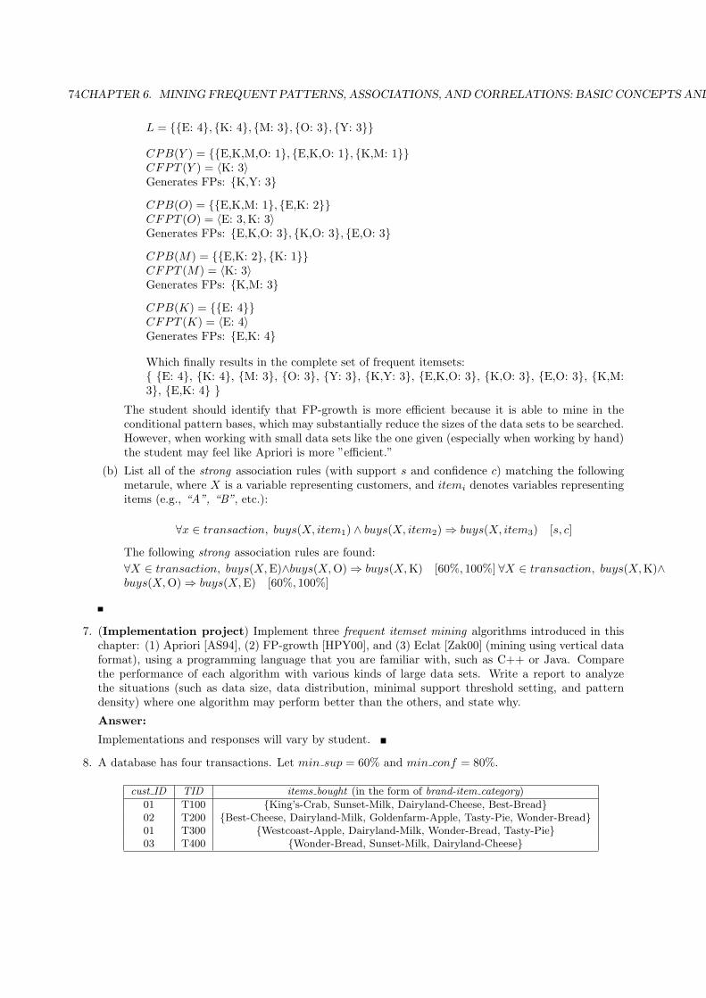
74CHAPTER 6. MINING FREQUENT PATTERNS, ASSOCIATIONS, AND CORRELATIONS: BASIC CONCEPTS ANDMETHODS
L = {{E: 4}, {K: 4}, {M: 3}, {O: 3}, {Y: 3}}
CPB(Y ) = {{E,K,M,O: 1}, {E,K,O: 1}, {K,M: 1}}CFPT (Y ) = ⟨K: 3⟩Generates FPs: {K,Y: 3}
CPB(O) = {{E,K,M: 1}, {E,K: 2}}CFPT (O) = ⟨E: 3,K: 3⟩Generates FPs: {E,K,O: 3}, {K,O: 3}, {E,O: 3}
CPB(M) = {{E,K: 2}, {K: 1}}CFPT (M) = ⟨K: 3⟩Generates FPs: {K,M: 3}
CPB(K) = {{E: 4}}CFPT (K) = ⟨E: 4⟩Generates FPs: {E,K: 4}
Which finally results in the complete set of frequent itemsets:{ {E: 4}, {K: 4}, {M: 3}, {O: 3}, {Y: 3}, {K,Y: 3}, {E,K,O: 3}, {K,O: 3}, {E,O: 3}, {K,M:3}, {E,K: 4} }
The student should identify that FP-growth is more efficient because it is able to mine in theconditional pattern bases, which may substantially reduce the sizes of the data sets to be searched.However, when working with small data sets like the one given (especially when working by hand)the student may feel like Apriori is more ”efficient.”
(b) List all of the strong association rules (with support s and confidence c) matching the followingmetarule, where X is a variable representing customers, and itemi denotes variables representingitems (e.g., “A”, “B”, etc.):
∀x ∈ transaction, buys(X, item1) ∧ buys(X, item2)⇒ buys(X, item3) [s, c]
The following strong association rules are found:
∀X ∈ transaction, buys(X,E)∧buys(X,O)⇒ buys(X,K) [60%, 100%] ∀X ∈ transaction, buys(X,K)∧buys(X,O)⇒ buys(X,E) [60%, 100%]
7. (Implementation project) Implement three frequent itemset mining algorithms introduced in thischapter: (1) Apriori [AS94], (2) FP-growth [HPY00], and (3) Eclat [Zak00] (mining using vertical dataformat), using a programming language that you are familiar with, such as C++ or Java. Comparethe performance of each algorithm with various kinds of large data sets. Write a report to analyzethe situations (such as data size, data distribution, minimal support threshold setting, and patterndensity) where one algorithm may perform better than the others, and state why.
Answer:
Implementations and responses will vary by student.
8. A database has four transactions. Let min sup = 60% and min conf = 80%.
cust ID TID items bought (in the form of brand-item category)
01 T100 {King’s-Crab, Sunset-Milk, Dairyland-Cheese, Best-Bread}02 T200 {Best-Cheese, Dairyland-Milk, Goldenfarm-Apple, Tasty-Pie, Wonder-Bread}01 T300 {Westcoast-Apple, Dairyland-Milk, Wonder-Bread, Tasty-Pie}03 T400 {Wonder-Bread, Sunset-Milk, Dairyland-Cheese}

6.1. EXERCISES 75
(a) At the granularity of item category (e.g., itemi could be “Milk”), for the following rule template,
∀X ∈ transaction, buys(X, item1) ∧ buys(X, item2)⇒ buys(X, item3) [s, c]
list the frequent k-itemset for the largest k, and all of the strong association rules (with theirsupport s and confidence c) containing the frequent k-itemset for the largest k.
(b) At the granularity of brand-item category (e.g., itemi could be “Sunset-Milk”), for the followingrule template,
∀X ∈ customer, buys(X, item1) ∧ buys(X, item2)⇒ buys(X, item3)
list the frequent k-itemset for the largest k (but do not print any rules).
Answer:
(a) At the granularity of item category (e.g., itemi could be “Milk”), for the following rule template,
∀X ∈ transaction, buys(X, item1) ∧ buys(X, item2)⇒buys(X, item3) [s, c]
list the frequent k-itemset for the largest k and all of the strong association rules (with theirsupport s and confidence c) containing the frequent k-itemset for the largest k.
k = 3 and the frequent 3-itemset is {Bread, Milk, Cheese}. The rules are
Bread ∧ Cheese⇒Milk, [75%, 100%]Chees ∧Milk ⇒ Bread, [75%, 100%]Chees⇒Milk ∧Bread, [75%, 100%]
(b) At the granularity of brand-item category (e.g., itemi could be “Sunset-Milk”), for the followingrule template,
∀X ∈ customer, buys(X, item1) ∧ buys(X, item2)⇒buys(X, item3)
list the frequent k-itemset for the largest k. Note: do not print any rules.
k = 3 and the frequent 3-itemset is {(Wheat-Bread, Dairyland-Milk, Tasty-Pie), (Wheat-Bread,Sunset-Milk, Dairyland-Cheese)}.
9. Suppose that a large store has a transactional database that is distributed among four locations.Transactions in each component database have the same format, namely Tj : {i1, . . . , im}, where Tj isa transaction identifier, and ik (1 ≤ k ≤ m) is the identifier of an item purchased in the transaction.Propose an efficient algorithm to mine global association rules. You may present your algorithm in theform of an outline. Your algorithm should not require shipping all of the data to one site and shouldnot cause excessive network communication overhead.
Answer:
An algorithm to mine global association rules is as follows:
• Find the local frequent itemsets in each store. Let CF be the union of all of the local frequentitemsets in the four stores.
• In each store, find the local (absolute) support for each itemset in CF .

76CHAPTER 6. MINING FREQUENT PATTERNS, ASSOCIATIONS, AND CORRELATIONS: BASIC CONCEPTS ANDMETHODS
• Now we must determine the global (absolute) support for each itemset in CF . This can be doneby summing up, for each itemset, the local support of that itemset in the four stores. Doing thisfor each itemset in CF will give us their global supports. Itemsets whose global supports passthe support threshold are global frequent itemsets.
• Derive strong association rules from the global frequent itemsets.
10. Suppose that frequent itemsets are saved for a large transactional database, DB. Discuss how toefficiently mine the (global) association rules under the same minimum support threshold, if a set ofnew transactions, denoted as ∆DB, is (incrementally) added in?
Answer:
We can treat ∆DB and DB as two partitions.
• For itemsets that are frequent in DB, scan ∆DB once and add their counts to see if they are stillfrequent in the updated database.
• For itemsets that are frequent in ∆DB but not in DB, scan DB once to add their counts to seeif they are frequent in the updated DB.
11. Most frequent pattern mining algorithms consider only distinct items in a transaction. However,multiple occurrences of an item in the same shopping basket, such as four cakes and three jugs ofmilk, can be important in transactional data analysis. How can one mine frequent itemsets efficientlyconsidering multiple occurrences of items? Propose modifications to the well-known algorithms, suchas Apriori and FP-growth, to adapt to such a situation.
Answer:
When extending the Apriori algorithm to mine frequent itemsets considering multiple occurrences ofitems, we need to take the count value into consideration when generating frequent items and itemsets.That is, we need to treat each item with different count value as different items (e.g., A:1 and A:2,that is, A with single count or 2 counts, as different items), and check if the minimal support is met.Then we can construct frequent 2-itemsets, 3-itemsets, etc., the same way as we do in Apriori. Weneed to take the count into consideration when checking the generated itemsets to decide if they areindeed frequent or not.
When extending the FPgrowth algorithm, we also need to take the count values into considerationwhen generating frequent items and itemsets. That is, when we do projected DBs, we will need toproject on the itemsets where each item can be associated with different counts. Further optimizationis possible in a similar way as mining closed itemsets.
12. (Implementation project) Many techniques have been proposed to further improve the performanceof frequent-itemset mining algorithms. Taking FP-tree-based frequent pattern-growth algorithms (suchas FP-growth) as an example, implement one of the following optimization techniques. Compare theperformance of your new implementation with the unoptimized version.
(a) The frequent pattern mining method of Section 6.2.4 uses an FP-tree to generate conditionalpattern bases using a bottom-up projection technique, i.e., project onto the prefix path of an itemp. However, one can develop a top-down projection technique, that is, project onto the suffixpath of an item p in the generation of a conditional pattern-base. Design and implement sucha top-down FP-tree mining method. Compare its performance with the bottom-up projectionmethod.

6.1. EXERCISES 77
(b) Nodes and pointers are used uniformly in an FP-tree in the design of the FP-growth algorithm.However, such a structure may consume a lot of space when the data are sparse. One possiblealternative design is to explore array-and pointer- based hybrid implementation, where a node maystore multiple items when it contains no splitting point to multiple sub-branches. Develop suchan implementation and compare it with the original one.
(c) It is time- and space- consuming to generate numerous conditional pattern bases during pattern-growth mining. An interesting alternative is to push right the branches that have been minedfor a particular item p, that is, to push them to the remaining branch(es) of the FP-tree. Thisis done so that fewer conditional pattern bases have to be generated and additional sharing canbe explored when mining the remaining branches of the FP-tree. Design and implement such amethod and conduct a performance study on it.
Answer:
Implementations and responses will vary by student.
13. Give a short example to show that items in a strong association rule may actually be negativelycorrelated.
Answer:
Consider the following table:
A A Σrow
B 65 35 100
B 40 10 50Σcol 105 35 150
Let the minimum support be 40%. Let the minimum confidence be 60%. A⇒B is a strong rulebecause it satisfies minimum support and minimum confidence with a support of 65/150 = 43.3% anda confidence of 65/100 = 61.9%. However, the correlation between A and B is corrA,B = 0.433
0.700×0.667= 0.928, which is less than 1, meaning that the occurrence of A is negatively correlated with theoccurrence of B.
14. The following contingency table summarizes supermarket transaction data, where hot dogs refers to thetransactions containing hot dogs, hotdogs refers to the transactions that do not contain hot dogs, ham-burgers refers to the transactions containing hamburgers, and hamburgers refers to the transactionsthat do not contain hamburgers.
hot dogs hotdogs Σrow
hamburgers 2000 500 2500
hamburgers 1000 1500 2500Σcol 3000 2000 5000
(a) Suppose that the association rule “hot dogs ⇒ hamburgers” is mined. Given a minimum supportthreshold of 25% and a minimum confidence threshold of 50%, is this association rule strong?
(b) Based on the given data, is the purchase of hot dogs independent of the purchase of hamburgers?If not, what kind of correlation relationship exists between the two?
(c) Compare the use of the all confidence, max confidence, Kulczynski, and cosine measures with liftand correlation on the given data.

78CHAPTER 6. MINING FREQUENT PATTERNS, ASSOCIATIONS, AND CORRELATIONS: BASIC CONCEPTS ANDMETHODS
Answer:
(a) Suppose that the association rule “hotdogs ⇒ hamburgers” is mined. Given a minimum supportthreshold of 25% and a minimum confidence threshold of 50%, is this association rule strong?
For the rule, support = 2000/5000 = 40%, and confidence = 2000/3000 = 66.7%. Therefore, theassociation rule is strong.
(b) Based on the given data, is the purchase of hotdogs independent of the purchase of hamburgers?If not, what kind of correlation relationship exists between the two?
corr{hotdog,hamburger} = P({hot dog, hamburger})/(P({hot dog}) P({hamburger}))=0.4/(0.5 ×0.6) = 1.33 > 1. So, the purchase of hotdogs is NOT independent of the purchase of hamburgers.There exists a POSITIVE correlation between the two.
15. (Implementation project) The DBLP data set (http://www.informatik.uni-trier.de/∼ley/db/) con-sists of over one million entries of research papers published in computer science conferences andjournals. Among these entries, there are a good number of authors that have coauthor relationships.
(a) Propose a method to efficiently mine a set of coauthor relationships that are closely correlated(e.g., often coauthoring papers together).
(b) Based on the mining results and the pattern evaluation measures discussed in this chapter, discusswhich measure may convincingly uncover close collaboration patterns better than others.
(c) Based on the study above, develop a method that can roughly predict advisor and advisee rela-tionships and the approximate period for such advisory supervision.
Answer: Implementations and responses will vary by student.
6.2 Supplementary Exercises
1. No question is added yet

Chapter 7
Advanced Pattern Mining
7.1 Exercises
1. Propose and outline a level-shared mining approach to mining multilevel association rules in whicheach item is encoded by its level position. Design it so that an initial scan of the database collects thecount for each item at each concept level, identifying frequent and subfrequent items. Comment on theprocessing cost of mining multilevel associations with this method in comparison to mining single-levelassociations.
Answer:
A level-shared mining approach is presented here, using the taxonomy of Figure 7.1 for illustration.
milk bread
2% chocolate white wheat
Dairy_land Wonder Old Mills Wonder
food
Wonder Foremost Foremost Dairy_land
Figure 7.1: A taxonomy of data items.
• Step 1: Scan the original transaction database. During the scan, create a hierarchy-information-encoded transaction table T of the database by encoding each item by its level position.
For the above example, the item “2% Foremost Milk” would be encoded as ‘112’. The first digit,1’, represents “milk” at level-1, the second digit, ‘1’, represents “2%” at level-2, and the thirddigit, ‘2’, represents “Foremost” at level-3. The item “Wonder White Bread” would be encodedas ‘212’.
79

80 CHAPTER 7. ADVANCED PATTERN MINING
Also during the scan, accumulate the support counts of each item at each concept level by exam-ining the encoded representation of each item. By doing so, we will discover the frequent items(1-itemsets) at all levels. Note that each level has its own minimum support threshold. Thesefrequent itemsets are frequent with respect to their level’s minimum support.
• Step 2: The initial database scan in Step 1 finds the frequent 1-itemsets, L1, at all levels.Join these frequent 1-itemsets to generate the candidate 2-itemsets at all levels. Scan T once todetermine which of the candidate 2-itemsets are frequent. Join the frequent 2-itemsets to generatethe candidate 3-itemsets at all levels. Scan T once to determine which of the candidate 3-itemsetsare frequent. Continue in this manner until none of the levels generate any new candidate itemsets.As we can see, this is basically the Apriori algorithm.
• Step 3: Once we have found all of the frequent itemsets of all the levels, generate the correspond-ing strong multilevel association rules.
Let’s compare the processing cost of mining multilevel associations with this method vs. miningsingle-level associations. A similarity is that the cost of database scans for this method is equal tothe cost of database scans for single-level associations. This is because, with one scan of the encodedtransaction table T , we collect the support counts for the current iteration’s candidate itemsets, at alllevels. Therefore, to determine the largest frequent k-itemsets at all levels, we only need to scan theencoded transaction table k times. However, this method must generate all of the current iteration’scandidate itemsets, for all levels, in order to collect all of their support counts in one scan of T .This is inefficient because some of these itemsets probably do not need to be generated (i.e., when anitemset’s corresponding ancestor candidate itemset is not frequent or subfrequent). Mining single-levelassociations, on the other hand, only involves generating candidate sets for one level. Therefore, thecost of generating candidates for this method is much greater than the cost of generating candidatesfor single-level associations.
2. Suppose, as manager of a chain of stores, you would like to use sales transactional data to analyze theeffectiveness of your store’s advertisements. In particular, you would like to study how specific factorsinfluence the effectiveness of advertisements that announce a particular category of items on sale. Thefactors to study are: the region in which customers live, and the day-of-the-week, and time-of-the-dayof the ads. Discuss how to design an efficient method to mine the transaction data sets and explainhow multidimensional and multilevel mining methods can help you derive a good solution.
Answer:
For handling this complex problem, both multidimensional and multilevel mining are useful tools.Because you are interested in analyzing the effects of your advertisment campaigns with respect tomultiple factors, it is clear that you must utilize multidimensional frequent pattern mining. Whenmining, you can mine patterns not only using the actual items bought (i.e., the buys predicate), but alsowith the location and time of the purchases. Utilizing all of these dimensions allows you to actually findpatterns that are a result of the targeted advertisement campaign you utilized. Furthermore, multilevelmining will be valuable for this task, especially with regard to mining locations. The hierarcthy forthe location data contains specific locations at the lowest level, and the advertisement regions at ahigher level. When mining, if frequent patterns are not discovered at the region level as a result ofthe advertisements, perhaps they can be found at a lower level, indicating that the advertisements forparticular product groups are particularly effective in certain locations. This knowledge would allowyou to define new regions in order to more effectively target your advertisements for maximum profit.
In designing an efficient algorithm to solve the following observations should be taken into consideration:
(a) The predicates (dimensions) being utilized should be buys, location, time

7.1. EXERCISES 81
(b) Reduced support at lower levels of the location heirarchy should be utilized. Because each storein a region may not represent a large enough portion of the total regional sales for a k-predicateset to become frequent.
(c) In this case, we are only interested in interdimensional association rules, we do not need to worryabout repeated predicates.
With this in mind, a data cube-based algorithm which mines at each level of the multiple concepthierarchies previously described ought to be identified as an efficient solution.
3. Quantitative association rulesmay disclose exceptional behaviors within a data set, where“exceptional”can be defined based on statistical theory. For example, Section 7.2.3 shows the association rule:
sex = female⇒ meanwage = $7.90/hr (overallmeanwage = $9.02/hr),
which suggests an exceptional pattern. The rule states that the average wage for females is only $7.90per hour, which is a significantly lower wage than the overall average of $9.02 per hour. Discusshow such quantitative rules can be discovered systematically and efficiently in large data sets withquantitative attributes.
Answer:
The following general ideas will allow us to efficiently find quantitative mean-based rules, the moregeneral case may be found in the reference material.
First, find all frequent sets of categorical items only, using known algorithms such as Apriori or FP-growth.
For all quantitative attribute, calculate the mean for each frequent set, using the hash-tree data struc-ture presented by Agrawal and Srikant. One pass over the database is sufficient.
Finally, find all non-contained rules and sub-rules. For every frequent set X and quantitative attributee, it remains to check if X ⇒Meane(TX) is a rule satisfying the statistical significance and minimumdifference requirements. This may be done by traversing a lattice of the frequent sets.
References: R. Agrawal and R. Srikant. Fast algorithms for mining association rules in large databases.Proc. of the 20th Intl. Conference on VLDB, 1994.
Y. Aumann and Y. Lindell. A statistical theory for quantitative association rules. Proc. of the 5thIntl. Conference on KDD, 1999.
4. In multidimensional data analysis, it is interesting to extract pairs of similar cell characteristics as-sociated with substantial changes in measure in a data cube, where cells are considered similar ifthey are related by roll-up (i.e, ancestors), drill-down (i.e, descendants), or 1-dimensional mutation(i.e, siblings) operations. Such an analysis is called cube gradient analysis. Suppose the measureof the cube is average. A user poses a set of probe cells and would like to find their correspondingsets of gradient cells, each of which satisfies a certain gradient threshold. For example, find the set ofcorresponding gradient cells whose average sale price is greater than 20% of that of the given probecells. Develop an algorithm than mines the set of constrained gradient cells efficiently in a large datacube.
Answer:
The following rudimentary algorithm, while not efficient, solves the problem: First, compute the icebergcube I from D using a significance constraint to reduce the number of interesting cells. Then select theset of significant probe cells, P , from I (using some sort of probe constaint). Finally, for each probe

82 CHAPTER 7. ADVANCED PATTERN MINING
cell cp ∈ P compute the set of gradient cells, and return those which satisfy the gradient constraint.A more efficient algorithm is discussed in the reference material.
Reference: G. Dong, J. Han, J. M. W. Lam, J. Pei, and K. Wang. Mining Multi-Dimensional Con-strained Gradients in Data Cubes. Proc. of the 27th Intl. Conference on VLDB, 2001.
5. Section 7.2.4 presented various ways of defining negatively correlated patterns. Consider Definition 3:“Suppose that itemsets X and Y are both frequent, that is, sup(X) ≥ min sup and sup(Y ) ≥ min sup,where min sup is the minimum support threshold. If (P (X|Y )+P (Y |X))/2 < ϵ, where ϵ is a negativepattern threshold, then pattern X ∪ Y is a negatively correlated pattern.” Design an efficientpattern-growth algorithm for mining the set of negatively correlated patterns.
Answer:
First, for each frequent item, construct its conditional pattern-base, and then its conditional FP-tree.Repeat the process on each newly created conditional FP-tree until the resulting FP-tree is empty,or it consaints only one path. As in FP-growth, a single path will generate all the combinationsof its sub-paths, each of which is a frequent pattern. Differing from FP-growth, at this stage wewant to store information about both frequent and infrequent patterns at this stage. Finally, foreach frequent itemset X, we scan the infrequent item sets Z, which contain X. Let Y = Z \ X,that is, Y contains the elements of Z which are not in X. If Y is a frequent item set, then wecalculate (P (X|Y )+P (Y |X))/2 = (sup(Z)/sup(Y )+ sup(Z)/sup(X))/2 to determine whether X andY are negatively correlated. Note that the support values sup(X), sup(Y ), and sup(Z) are all storedpreviously in the algorithm.
6. Prove that each entry in the following table correctly characterizes its corresponding rule constraintfor frequent itemset mining.
Rule constraint Antimonotonic Monotonic Succinct
a) v ∈ S no yes yesb) S ⊆ V yes no yesc) min(S) ≤ v no yes yesd) range(S) ≤ v yes no noe) variance(S) ≤ v convertible convertible no
Answer:
(a) v ∈ S: not antimonotone, but monotone, succinct.
Answer:
• Antimonotone:Proof by a counter-example: Let v = 5 and S = {1, 2, 3}. Now v ∈ S is false. By adding 5 toS, v ∈ S is true. Thus v ∈ S is not an anti-monotone constraint.
• Monotone:Proof: Let v ∈ S. Let S′ be a superset of S, that is, every element of S must be an element inS′. Assume that v ∈ S′. Then S′ cannot be a superset of S because it does not contain everyelement of S. But S′ is a superset of S. This is a contradiction. Thus, v ∈ S′. Therefore,v ∈ S is a monotone constraint.
• Succinct:Proof: v ∈ S is a succinct constraint because we can explicitly and precisely generate all thesets of items satisfying the constraint. Specifically, such a set S must contain the element v.
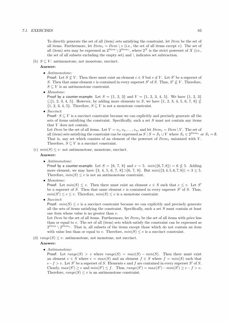
7.1. EXERCISES 83
To directly generate the set of all (item) sets satisfying the constraint, let Item be the set ofall items. Furthermore, let Item1 = Item \ v (i.e., the set of all items except v). The set ofall (item) sets may be expressed as 2Item \ 2Item1 , where 2X is the strict powerset of X (i.e.,the set of all subsets excluding the empty set) and \ indicates set subtraction.
(b) S ⊆ V : antimonotone, not monotone, succinct.
Answer:
• Antimonotone:Proof: Let S ⊆ V . Then there must exist an element e ∈ S but e ∈ V . Let S′ be a superset ofS. Then that same element e is contained in every superset S′ of S. Thus, S′ ⊆ V . Therefore,S ⊆ V is an antimonotone constraint.
• Monotone:Proof by a counter-example: Let S = {1, 2, 3} and V = {1, 2, 3, 4, 5}. We have {1, 2, 3}⊆{1, 2, 3, 4, 5}. However, by adding more elements to S, we have {1, 2, 3, 4, 5, 6, 7, 8} ⊆{1, 2, 3, 4, 5}. Therefore, S ⊆ V is not a monotone constraint.
• Succinct:Proof: S ⊆ V is a succinct constraint because we can explicitly and precisely generate all thesets of items satisfying the constraint. Specifically, such a set S must not contain any itemsthat V does not contain.Let Item be the set of all items. Let V = v1, v2, . . . , vn, and let Item1 = Item\V . The set ofall (item) sets satisfying the constraint can be expressed as S | S = S1 ∪ V where S1 ∈ 2Item1 or S1 = ∅.That is, any set which consists of an element of the powerset of Item1 unionized with V .Therefore, S ⊆ V is a succinct constraint.
(c) min(S) ≤ v: not antimonotone, monotone, succinct.
Answer:
• Antimonotone:Proof by a counter-example: Let S = {6, 7, 8} and v = 5. min({6, 7, 8}) = 6 � 5. Addingmore element, we may have {3, 4, 5, 6, 7, 8}⊃{6, 7, 8}. But min({3, 4, 5, 6, 7, 8}) = 3 ≤ 5.Therefore, min(S) ≤ v is not an antimonotone constraint.
• Monotone:Proof: Let min(S) ≤ v. Then there must exist an element e ∈ S such that e ≤ v. Let S′
be a superset of S. Then that same element e is contained in every superset S′ of S. Thus,min(S′) ≤ e ≤ v. Therefore, min(S) ≤ v is a monotone constraint.
• Succinct:Proof: min(S) ≤ v is a succinct constraint because we can explicitly and precisely generateall the sets of items satisfying the constraint. Specifically, such a set S must contain at leastone item whose value is no greater than v.Let Item be the set of all items. Furthermore, let Item1 be the set of all items with price lessthan or equal to v. The set of all (item) sets which satisfy the constraint can be expressed as2Item \ 2Item1 . That is, all subsets of the items except those which do not contain an itemwith value less than or equal to v. Therefore, min(S) ≤ v is a succinct constraint.
(d) range(S) ≤ v: antimonotone, not monotone, not succinct.
Answer:
• Antimonotone:Proof: Let range(S) > v where range(S) = max(S) − min(S). Then there must existan element e ∈ S where e = max(S) and an element f ∈ S where f = min(S) such thate−f > v. Let S′ be a superset of S. Elements e and f are contained in every superset S′ of S.Clearly, max(S′) ≥ e and min(S′) ≤ f . Thus, range(S′) = max(S′)−min(S′) ≥ e− f > v.Therefore, range(S) ≤ v is an antimonotone constraint.

84 CHAPTER 7. ADVANCED PATTERN MINING
• Monotone:Proof by a counter-example: Let S = {4, 5, 6} and v = 5. range({4, 5, 6}) = 6 − 4 =2 < 5. By adding some more elements, such as {1, 2, 3, 4, 5, 6, 7, 8} ⊃ {1, 2, 3}. However,range({1, 2, 3, 4, 5, 6, 7, 8}) = 8 − 1 = 7 � 5. Therefore, range(S) ≤ v is not a monotoneconstraint.
• Not Succinct:Proof by a counter-example: range(S) ≤ v is not a succinct constraint because we can-not explicitly and precisely generate all the sets of items satisfying the constraint. It de-pends on the maximum and the minimum of the set. For example: range(5, 6, 7) = 2 butrange(4, 5, 6, 7, 8) = 2. We cannot prune 4 or 8 from the original set of items because theymay satisfy the constraint too, e.g., range(4, 5, 6) = 2 and range(6, 7, 8) = 2. Thus, we mustuse the “generate-and-test” approach at each iteration. Therefore, range(S) ≤ v is not asuccinct constraint.
(e) avg(S) ≤ v: Convertible Antimonotone, Convertible Monotone, Not Succinct.
Answer:
• Convertible Antimonotone:Proof: Let R be the value-ascending order over the set of items I so that items in a transactionare added to an itemset in value-ascending order. Let avg(S) ≥ v. Let S′ be a superset of S.Then there must exist some S′′ such that (i) S′ = S ∪ S′′ and (ii) each item in S′′ is greaterthan every item in S. Clearly then, avg(S′) ≥ v because adding increasingly more expensiveitems will only make the average price increase. Therefore, avg(S) ≤ v is a convertibleantimonotone constraint.
• Convertible Monotone:Proof: Let R be the value-descending order over the set of items I so that items in a transac-tion are added to an itemset in value-descending order. Let avg(S) ≤ v. Let S′ be a supersetof S. Let S′ be a superset of S. Then there must exist some S′′ such that (i) S′ = S∪S′′ and(ii) each item in S′′ is less than every item in S. Clearly then, avg(S′) ≤ v because addingdecreasingly cheap items will only make the average price decrease. Therefore, avg(S) ≤ v isa convertible monotone constraint.
• Not Succinct:Proof by a counter-example: avg(S) ≤ v is not a succinct constraint because we cannotexplicitly and precisely generate all the sets of items satisfying the constraint. It depends onitems in the set. For example: avg(6, 50) = 28 � 10. We cannot prune 50 from the originalset of items because it may satisfy the constraint too, e.g., avg(1, 2, 3, 4, 5, 6, 7, 8, 9, 10, 50) =9.5 ≤ 10. Thus, we must use the “generate-and-test” approach at each iteration.
7. The price of each item in a store is nonnegative. The store manager is only interested in rules ofcertain forms, using the constraints given below. For each of the following cases, identify the kinds ofconstraint they represent and briefly discuss how to mine such association rules using constraint-based pattern mining.
(a) Containing at least one Blueray DVD movie
(b) Containing items whose sum of the prices is less than $150
(c) Containing one free item and other items whose sum of the prices is at least $200
(d) Where the average price of all the items is between $100 and $500
Answer:

7.1. EXERCISES 85
(a) Containing at least one Blueray DVD movie
The constraint is succinct and monotonic. This constraint can be mined efficiently using FP-growth as follows.
• All frequent Nintendo games are listed at the end of the list of frequent items L.
• Only those conditional pattern bases and FP-trees for frequent Blueray DVD movie need tobe derived from the global FP-tree and mined recursively.
(b) Containing items whose sum of the prices is less than $150
The constraint is antimonotonic. This constraint can be mined efficiently using Apriori as follows.Only candidates with sum of prices less than $150 need to be checked.
(c) Containing one free item and other items whose sum of the prices is at least $200 in total.
The constraint “containing one free item” is succinct, whereas the constraint “sum of the pricesis at least $200 in total” is monotonic and data antimonotonic. It can be mined efficiently usingFP-growth as follows.
• Put all frequent free items at the end of the list of frequent items L (i.e., they will be pushedin first in mining)
• Only conditional pattern bases and FP-trees for frequent free items need to be derived fromthe global FP-tree and mined recursively. Other free items should be excluded from theseconditional pattern bases and FP-trees.
• Once a pattern with sum of the price is at least $200, no further constraint checking for totalprice is needed in recursive mining.
• A pattern as well as its conditional pattern base can be pruned, if the sum of the price ofitems in the pattern and the frequent ones in the pattern base is less than $200 (based on theproperty of data anti-monotonicity).
(d) Where the average price of all the items is between $100 and $150.
The sub-constraints ”the average price is at least $100” and ”the average price is at most $500”are convertible. It can be mined efficiently using FP-growth as follows.
• All the frequent items are listed in price descending order; (if you use ascending order, youmust rewrite the following two steps.)
• A pattern as well as its conditional pattern base can be pruned, if the average price of itemsin the pattern and those frequent ones in pattern base with prices greater than $100 is lessthan $100.
• A pattern as well as its conditional pattern base can also be pruned, if the average price ofitems in the pattern is greater than $500.
8. Section 7.4.1 introduced a core-pattern-fusion method for mining high-dimensional data. Explainwhy a long pattern, if exists in the data set, is likely to be discovered by this method.
Answer:
The core Pattern-Fusion method utilizes the concept of core patterns to effectively discover colossalpatterns. Not only do colossal patterns have far more core descendants than small patterns, but theyhave far more core patterns that are close to one another than small patterns. Therefore, the Pattern-Fusion method of discovering close core patterns and fusing them together has a high probability todetect any colossal pattern which exists.
9. Section 7.5.1 defined a pattern distance measure between closed patterns P1 and P2 as
Pat Dist(P1, P2) = 1− |T (P1) ∩ T (P2)||T (P1) ∪ T (P2)|
,

86 CHAPTER 7. ADVANCED PATTERN MINING
where T (P1) and T (P2) are the supporting transaction sets of P1 and P2, respectively. Is this a validdistance metric? Show the derivation to support your answer.
Answer:
The distance measure Pat Dist is a valid distance metric. It has the following properties:
(a) Pat Dist(P1, P2) > 0, ∀P1 = P2
(b) Pat Dist(P1, P2) = 0, ∀P1 = P2
(c) Pat Dist(P1, P2) = Pat Dist(P2, P1)
(d) Pat Dist(P1, P2) + Pat Dist(P2, P3) ≥ Pat Dist(P1, P3), ∀P1, P2, P3
Since (T (P1) ∩ T (P2)) ∪ (T (P1) ∩ T (P3)) ⊆ T (P1), we have
|T (P1) ∩ T (P2)|+ |T (P1) ∩ T (P3)|−|T (P1) ∩ T (P2) ∩ T (P3)| ≤ |T (P1)|
=⇒ b1 + c1 − d1 ≤ a (7.1)
Plug in all the variables into the distance definition,
Pat Dist(P1, P2) + Pat Dist(P2, P3) ≥ Pat Dist(P1, P3)
⇐⇒ b1a+b2
+ c1a+c2
≤ 1 + d1+d2
b1+b2+c1+c2−d1−d2
Using Eq. (7.1), we have:
1 + d1+d2
b1+b2+c1+c2−d1−d2
≥ 1 + d1
b1+b2+c1+c2−d1(d2 ≥ 0)
≥ 1 + d1
a+b2+c2(Eq.??)
= a+d1+b2+c2a+b2+c2
≥ b1+c1+b2+c2a+b2+c2
(Eq.??)
= b1+c2a+b2+c2
+ c1+b2a+b2+c2
≥ b1a+b2
+ c1a+c2
(a+ b2 ≥ b1, c2 ≥ 0)
(a+ c2 ≥ c1, b2 ≥ 0)
Thus the fourth statement is true. This distance measure can be extended to general frequent patternsexcept that for non-closed patterns, we may have Pat Dist(P1, P2) = 0 for some P1 = P2. Thishappens when P1 and P2 share the same support transaction set.
10. Association rule mining often generates a large number of rules, many of which may be similar, thusnot containing much novel information. Design an efficient algorithm that compresses a large setof patterns into a small compact set. Discuss whether your mining method is robust under differentpattern similarity definitions.
Answer:
To compress a large set of patterns into a smaller set of representative patterns we can utilize aclustering based method. In order to do this we may use the concept of δ-clusters introduced inSection 7.5.1. One option is to implement a greedy algorithm to find the representatives which δ-coverthe most other patterns globally, but this method is not efficient and will fail when the number offrequent patterns increases. Another option is to use a locally greedy method which will have a worse

7.1. EXERCISES 87
result, but is more efficient. To achieve the best result, combining the globally greedy method withthe locally greedy method has shown to be efficient.
Reference: D. Xin, J. Han, X. Yan, and H. Cheng. On compressing frequent patterns. Data Knowl.Eng. 60, 1 (January 2007), 5-29.
11. Frequent pattern mining may generate many superfluous patterns. Therefore, it is important to developmethods that mine compressed patterns. Suppose a user would like to obtain only k patterns (where kis a small integer). Outline an efficient method that generates the k most representative patterns,where more distinct patterns are preferred over very similar patterns. Illustrate the effectiveness ofyour method using a small data set.
Answer:
In order to solve this problem efficiently we will use a redundancy graph G created based on the patternswhich have been mined. Within this weighted graph, each node represents a pattern and the weight ofeach node is the significance of the pattern represented. The weight of an edge between pi and pj is theredundancy, R(pi, pj). We are interested in evaluating subgraphs of G which contain k nodes based ontheir significance and redundancy. In general, it is very difficult to formulate the function returningredundancies among the patterns represented by a subgraph. In order to deal with this we must utilizea heuristic evaluation function. One such method would be to compute the maximum spanning tree,and use the sum of the weights in said tree to represent the redundancy. The problem now is to finda k-maximum spanning tree whose overall weights are minimized, but this problem has been shownto be NP-hard. However, we may use a greedy algorithm which incrementally selects patterns fromthe pattern set which have the maximum estimated gain among the remaining patterns. The resultset is initialized with the most significant pattern and the process repeats until k patterns have beenselected.
Reference: D. Xin, H. Cheng, X. Yan, and J. Han. Extracting redundancy-aware top-k patterns. Proc.of the 12th Intl. Conference on KDD, 2006.
12. It is interesting to generate semantic annotations for mined patterns. Section 7.6.1 presented apattern annotation method. Alternative methods are possible, such as by utilizing type information.In the DBLP data set, for example, authors, conferences, terms, and papers form multiple typeddata. Develop a method for automated semantic pattern annotation that makes good use of typedinformation.
Answer:
To incorporate type information into semantice annotation, we may use an extension of the methoddescribed in the chapter. By modifying the manner in which context units are chosen and allowingfor different weighting functions, user or expert specified information related to the types of objects inthe patterns being annotated can be incorporated. For example, when considering a subset of DBLPperhaps the user knows that the venues represented contain papers from many subfields and thereforechooses to enforce a reduction in the weight of any context unit containing a venue as they will containless semantic information. Alternatively, they may choose to not allow context units containing venues,accomplishing a similar goal. Because these extensions are covered well by the method described inthe chapter, no further development is necessary.
Reference: Q. Mei, D. Xin, H. Cheng, J. Han, and C. Zhai. Semantic annotation of frequent patterns.ACM Trans. Knowl. Discov. Data 1, 3, Article 11 (December 2007).

88 CHAPTER 7. ADVANCED PATTERN MINING
7.2 Supplementary Exercises
1. Suppose that a data relation describing students at Big-University has been generalized to the gener-alized relation R in Table 7.1.
Table 7.1: Generalized relation for Exercise 5.9.
major status age nationality gpa count
French M.A over 30 Canada 2.8 3.2 3cs junior 16...20 Europe 3.2 3.6 29
physics M.S 26...30 Latin America 3.2 3.6 18engineering Ph.D 26...30 Asia 3.6 4.0 78philosophy Ph.D 26...30 Europe 3.2 3.6 5French senior 16...20 Canada 3.2 3.6 40
chemistry junior 21...25 USA 3.6 4.0 25cs senior 16...20 Canada 3.2 3.6 70
philosophy M.S over 30 Canada 3.6 4.0 15French junior 16...20 USA 2.8 3.2 8
philosophy junior 26...30 Canada 2.8 3.2 9philosophy M.S 26...30 Asia 3.2 3.6 9French junior 16...20 Canada 3.2 3.6 52math senior 16...20 USA 3.6 4.0 32cs junior 16...20 Canada 3.2 3.6 76
philosophy Ph.D 26...30 Canada 3.6 4.0 14philosophy senior 26...30 Canada 2.8 3.2 19French Ph.D over 30 Canada 2.8 3.2 1
engineering junior 21...25 Europe 3.2 3.6 71math Ph.D 26...30 Latin America 3.2 3.6 7
chemistry junior 16...20 USA 3.6 4.0 46engineering junior 21...25 Canada 3.2 3.6 96
French M.S over 30 Latin America 3.2 3.6 4philosophy junior 21...25 USA 2.8 3.2 8
math junior 16...20 Canada 3.6 4.0 59
Let the concept hierarchies be as follows:
status : {freshman, sophomore, junior, senior} ∈ undergraduate.{M.Sc.,M.A., Ph.D.} ∈ graduate.
major : {physics, chemistry,math} ∈ science.{cs, engineering} ∈ appl. sciences.{French, philosophy} ∈ arts.
age : {16...20, 21...25} ∈ young.{26...30, over 30} ∈ old.
nationality : {Asia,Europe, Latin America} ∈ foreign.{U.S.A., Canada} ∈ North America.
Let the minimum support threshold be 20% and the minimum confidence threshold be 50% (at eachof the levels).

7.2. SUPPLEMENTARY EXERCISES 89
(a) Draw the concept hierarchies for status, major, age, and nationality.
(b) Write a program to find the set of strong multilevel association rules in R using uniform supportfor all levels, for the following rule template,
∀S ∈ R, P (S, x) ∧Q(S, y)⇒ gpa(S, z) [s, c]
where P,Q ∈ {status,major, age, nationality}.(c) Use the program to find the set of strong multilevel association rules in R using level-cross filtering
by single items. In this strategy, an item at the ith level is examined if and only if its parentnode at the (i− 1)th level in the concept hierarchy is frequent. That is, if a node is frequent, itschildren will be examined; otherwise, its descendants are pruned from the search. Use a reducedsupport of 10% for the lowest abstraction level, for the preceding rule template.
Answer:
(a) Draw the concept hierarchies for status, major, age, and nationality.
See Figure 7.2.
Figure 7.2: Concept hierarchies
(b) Find the set of strong multilevel association rules in R using uniform support for all levels.
status(X, “undergraduate”) ∧ major(X, “science”) ⇒ gpa(X, “3.6...4.0”) [20% 100%]status(X, “undergraduate”) ∧ major(X, “appl sciences”) ⇒ gpa(X, “3.2...3.6”) [43%, 100%]status(X, “undergraduate”) ∧ age(X, “young”) ⇒ gpa(X, “3.2...3.6”) [55%, 71%]status(X, “undergraduate”) ∧ nationality(X, “North America”) ⇒ gpa(X, “3.2...3.6”) [42%, 62%]major(X, “science”) ∧ nationality(X, “North America”) ⇒ gpa(X, “3.6...4.0”) [20%, 100%]major(X, “appl sciences”) ∧ nationality(X, “North America”) ⇒ gpa(X, “3.2...3.6”) [31%, 100%]major(X, “science”) ∧ age(X, “young”) ⇒ gpa(X, “3.6...4.0”) [20%, 100%]major(X, “appl sciences”) ∧ age(X, “young”) ⇒ gpa(X, “3.2...3.6”) [43%, 100%]age(X, “young”) ∧ nationality(X, “North America”) ⇒ gpa(X, “3.2...3.6”) [42%, 65%]status(X, “junior”) ⇒ major(X, “engineering”) ⇒ gpa(X, “3.2...3.6”) [21% 100%]status(X, “junior”) ∧ age(X, 21...25) ⇒ gpa(X, “3.2...3.6”) [21%, 83.5%]status(X, “junior”) ∧ nationality(X, “Canada”) ⇒ gpa(X, “3.2...3.6”) [28%, 77%]major(X, “engineering”) ∧ age(X, 21...25) ⇒ gpa(X, “3.2...3.6”) [21%, 100%]age(X, 16...20) ∧ nationality(X, “Canada”) ⇒ gpa(X, “3.2...3.6”) [30%, 80%]
(c) Find the set of strong multilevel association rules in R using level-cross filtering by single items,where a reduced support of 1% is used for the lowest abstraction level.
Note: The following set of rules is mined in addition to those mined above.
status(X, “junior”) ∧ age(X, “16...20”)⇒gpa(X, “3.2...3.6”) [20%, 58%]status(X, “senior”) ∧ age(X, “16...20”)⇒gpa(X, “3.6...4.0”) [14%, 77%]status(X, “PhD”)age(X, “26...30”) ∧⇒gpa(X, “3.6...4.0”) [12%, 100%]status(X, “junior”) ∧ nationality(X, “Europe”)⇒gpa(X, “3.2...3.6”) [13%, 100%]status(X, “senior”) ∧ nationality(X, “Canada”)⇒gpa(X, “3.2...3.6”) [14%, 85%]major(X, “math”) ∧ age(X, 16...20)⇒gpa(X, “3.6...4.0”) [11%, 100%]major(X, “French”) ∧ age(X, 16...20)⇒gpa(X, “3.2...3.6”) [12%, 92%]major(X, “cs”) ∧ nationality(X, “Canada”)⇒gpa(X, “3.2...3.6”) [18%, 100%]

90 CHAPTER 7. ADVANCED PATTERN MINING
major(X, “engineering”) ∧ nationality(X, “Canada”)⇒gpa(X, “3.2...3.6”) [12%, 100%]major(X, “French”) ∧ nationality(X, “Canada”)⇒gpa(X, “3.2...3.6”) [12%, 96%]age(X, 21...25) ∧ nationality(X, “Canada”)⇒gpa(X, “3.2...3.6”) [12%, 100%]
2. The price of each item in a store is nonnegative. The store manager is only interested in rules of theform: “one free item may trigger $200 total purchases in the same transaction”. State how to minesuch rules efficiently using constraint-based pattern mining.
Answer:
To efficiently mine rules of the form “one free item may trigger $200 total purchases in the sametransaction”, we need to:
• Find the set of frequent ”free” 1-itemsets. Let us call this set S1.
• Generate the set of frequent itemsets whose price is no less than $200, using FP-growth. Let uscall this set S2.
This is a monotone constraint so we do not have to use the “generate-and-test” approach at eachiteration, which will save us some unnecessary computation. If we have a frequent itemset whoseprice is at least $200, then we do not need to check the constraint for any superset of that itemset.This is because any additional items added to the itemset will only increase the price total, whichis already at least $200. All that needs to be checked is if that superset is frequent.
The reason that we use FP-growth and not Apriori is because Apriori discards frequent itemsetswhose price is less than $200, and therefore is not be able to discover supersets of these itemsetsthat satisfy the constraint. FP-growth does not suffer from this problem because it keeps all ofthe information about the database in a tree structure.
• Find the frequent itemsets from the set S1S2, where S1 is the set of frequent ”free” 1-itemsetsand where S2 is the set of frequent itemsets whose price is no less than $200.
• Generate rules of the form S1⇒S2 from the frequent itemsets found above that meet the minimumconfidence threshold.

Chapter 8
Classification: Basic Concepts
8.1 Exercises
1. Briefly outline the major steps of decision tree classification.
Answer: The major steps are as follows:
• The tree starts as a single root node containing all of the training tuples.
• If the tuples are all from the same class, then the node becomes a leaf, labeled with that class.
• Else, an attribute selection method is called to determine the splitting criterion. Such a methodmay using a heuristic or statistical measure (e.g., information gain, gain ratio or gini index) toselect the “best” way to separate the tuples into individual classes. The splitting criterion consistsof a splitting attribute and may also indicate either a split-point or a splitting subset, as describedbelow.
• Next, the node is labeled with the splitting criterion, which serves as a test at the node. Abranch is grown from the node to each of the outcomes of the splitting criterion and the tuplesare partitioned accordingly. There are three possible scenarios for such partitioning. (1) If thesplitting attribute is discrete-valued, then a branch is grown for each possible value of the attribute.(2) If the splitting attribute, A, is continuous-valued, then two branches are grown, correspondingto the conditions A ≤ split point and A > split point. (3) If the splitting attribute is discrete-valued and a binary tree must be produced (e.g., if the gini index was used as a selection measure),then the test at the node is “A ∈ SA?” where SA is the splitting subset for A. It is a subset ofthe known values of A. If a given tuple has value aj of A and if aj ∈ SA, then the test at thenode is satisfied.
• The algorithm recurses to create a decision tree for the tuples at each partition.
The stopping conditions are:
• If all tuples at a given node belong to the same class, then transform that node into a leaf, labeledwith that class.
• If there are no more attributes left to create more partitions, then majority voting can be used toconvert the given node into a leaf, labeled with the most common class among the tuples.
• If there are no tuples for a given branch, a leaf is created with the majority class from the parentnode.
91

92 CHAPTER 8. CLASSIFICATION: BASIC CONCEPTS
2. Why is tree pruning useful in decision tree induction? What is a drawback of using a separate set oftuples to evaluate pruning?
Answer:
The decision tree built may overfit the training data. There could be too many branches, some ofwhich may reflect anomalies in the training data due to noise or outliers. Tree pruning addresses thisissue of overfitting the data by removing the least reliable branches (using statistical measures). Thisgenerally results in a more compact and reliable decision tree that is faster and more accurate in itsclassification of data.
The drawback of using a separate set of tuples to evaluate pruning is that it may not be representative ofthe training tuples used to create the original decision tree. If the separate set of tuples are skewed, thenusing them to evaluate the pruned tree would not be a good indicator of the pruned tree’s classificationaccuracy. Furthermore, using a separate set of tuples to evaluate pruning means there are less tuplesto use for creation and testing of the tree. While this is considered a drawback in machine learning, itmay not be so in data mining due to the availability of larger data sets.
3. Given a decision tree, you have the option of (a) converting the decision tree to rules and then pruningthe resulting rules, or (b) pruning the decision tree and then converting the pruned tree to rules. Whatadvantage does (a) have over (b)?
Answer:
If pruning a subtree, we would remove the subtree completely with method (b). However, with method(a), if pruning a rule, we may remove any precondition of it. The latter is less restrictive.
4. It is important to calculate the worst-case computational complexity of the decision tree algorithm.Given data set D, the number of attributes n, and the number of training tuples |D|, show that thecomputational cost of growing a tree is at most n× |D| × log(|D|).Answer:
The worst-case scenario occurs when we have to use as many attributes as possible before being ableto classify each group of tuples. The maximum depth of the tree is log(|D|). At each level we willhave to compute the attribute selection measure O(n) times (one per attribute). The total number oftuples on each level is |D| (adding over all the partitions). Thus, the computation per level of the treeis O(n× |D|). Summing over all of the levels we obtain O(n× |D| × log(|D|)).
5. Given a 5 GB data set with 50 attributes (each containing 100 distinct values) and 512 MB of mainmemory in your laptop, outline an efficient method that constructs decision trees in such large datasets. Justify your answer by rough calculation of your main memory usage.
Answer:
We will use the RainForest algorithm for this problem. Assume there are C class labels. The mostmemory required will be for AVC-set for the root of the tree. To compute the AVC-set for the rootnode, we scan the database once and construct the AVC-list for each of the 50 attributes. The sizeof each AVC-list is 100 × C. The total size of the AVC-set is then 100 × C × 50, which will easily fitinto 512MB of memory for a reasonable C. The computation of other AVC-sets is done in a similarway but they will be smaller because there will be less attributes available. To reduce the number ofscans we can compute the AVC-set for nodes at the same level of the tree in parallel. With such smallAVC-sets per node, we can probably fit the level in memory.
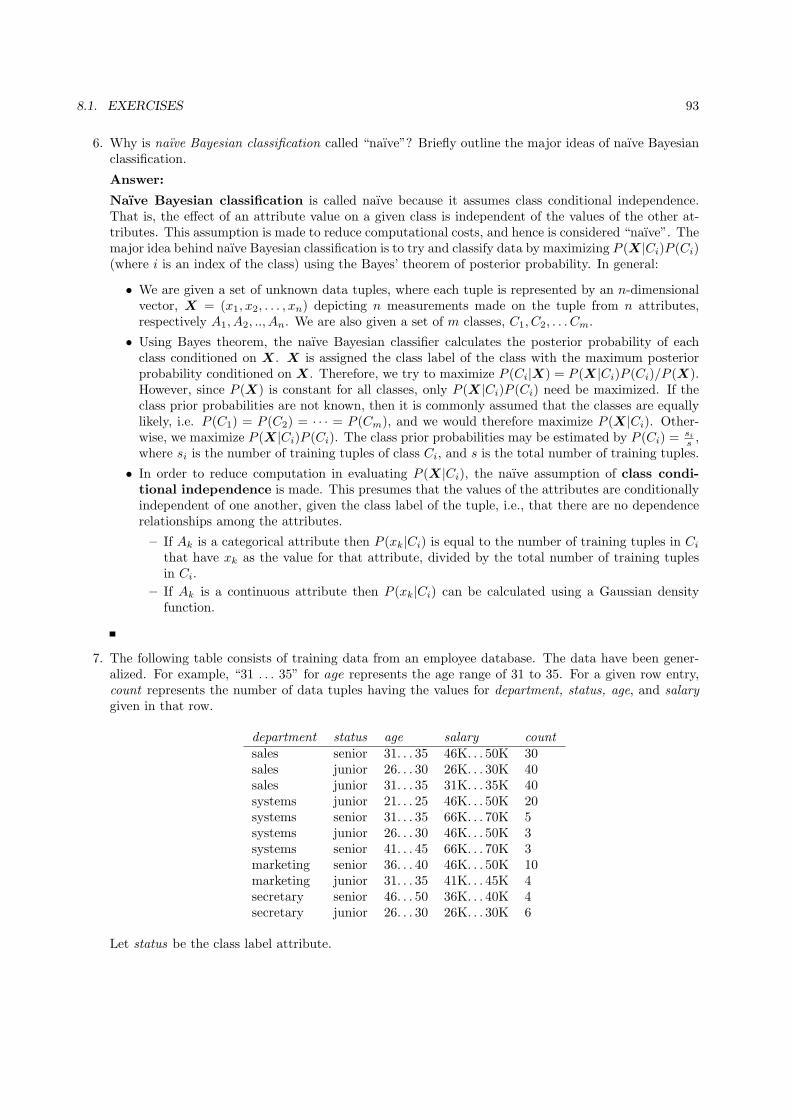
8.1. EXERCISES 93
6. Why is naıve Bayesian classification called “naıve”? Briefly outline the major ideas of naıve Bayesianclassification.
Answer:
Naıve Bayesian classification is called naıve because it assumes class conditional independence.That is, the effect of an attribute value on a given class is independent of the values of the other at-tributes. This assumption is made to reduce computational costs, and hence is considered “naıve”. Themajor idea behind naıve Bayesian classification is to try and classify data by maximizing P (X|Ci)P (Ci)(where i is an index of the class) using the Bayes’ theorem of posterior probability. In general:
• We are given a set of unknown data tuples, where each tuple is represented by an n-dimensionalvector, X = (x1, x2, . . . , xn) depicting n measurements made on the tuple from n attributes,respectively A1, A2, .., An. We are also given a set of m classes, C1, C2, . . . Cm.
• Using Bayes theorem, the naıve Bayesian classifier calculates the posterior probability of eachclass conditioned on X. X is assigned the class label of the class with the maximum posteriorprobability conditioned on X. Therefore, we try to maximize P (Ci|X) = P (X|Ci)P (Ci)/P (X).However, since P (X) is constant for all classes, only P (X|Ci)P (Ci) need be maximized. If theclass prior probabilities are not known, then it is commonly assumed that the classes are equallylikely, i.e. P (C1) = P (C2) = · · · = P (Cm), and we would therefore maximize P (X|Ci). Other-wise, we maximize P (X|Ci)P (Ci). The class prior probabilities may be estimated by P (Ci) =
sis ,
where si is the number of training tuples of class Ci, and s is the total number of training tuples.
• In order to reduce computation in evaluating P (X|Ci), the naıve assumption of class condi-tional independence is made. This presumes that the values of the attributes are conditionallyindependent of one another, given the class label of the tuple, i.e., that there are no dependencerelationships among the attributes.
– If Ak is a categorical attribute then P (xk|Ci) is equal to the number of training tuples in Ci
that have xk as the value for that attribute, divided by the total number of training tuplesin Ci.
– If Ak is a continuous attribute then P (xk|Ci) can be calculated using a Gaussian densityfunction.
7. The following table consists of training data from an employee database. The data have been gener-alized. For example, “31 . . . 35” for age represents the age range of 31 to 35. For a given row entry,count represents the number of data tuples having the values for department, status, age, and salarygiven in that row.
department status age salary countsales senior 31. . . 35 46K. . . 50K 30sales junior 26. . . 30 26K. . . 30K 40sales junior 31. . . 35 31K. . . 35K 40systems junior 21. . . 25 46K. . . 50K 20systems senior 31. . . 35 66K. . . 70K 5systems junior 26. . . 30 46K. . . 50K 3systems senior 41. . . 45 66K. . . 70K 3marketing senior 36. . . 40 46K. . . 50K 10marketing junior 31. . . 35 41K. . . 45K 4secretary senior 46. . . 50 36K. . . 40K 4secretary junior 26. . . 30 26K. . . 30K 6
Let status be the class label attribute.

94 CHAPTER 8. CLASSIFICATION: BASIC CONCEPTS
(a) How would you modify the basic decision tree algorithm to take into consideration the count ofeach generalized data tuple (i.e., of each row entry)?
(b) Use your algorithm to construct a decision tree from the given data.
(c) Given a data tuple having the values “systems”, “26. . . 30”, and “46–50K” for the attributesdepartment, age, and salary, respectively, what would a naıve Bayesian classification of the statusfor the tuple be?
Answer:
(a) How would you modify the basic decision tree algorithm to take into consideration the count ofeach generalized data tuple (i.e., of each row entry)?
The basic decision tree algorithm should be modified as follows to take into consideration thecount of each generalized data tuple.
• The count of each tuple must be integrated into the calculation of the attribute selectionmeasure (such as information gain).
• Take the count into consideration to determine the most common class among the tuples.
(b) Use your algorithm to construct a decision tree from the given data.
The resulting tree is:
(salary = 26K...30K:junior
= 31K...35K:junior
= 36K...40K:senior
= 41K...45K:junior
= 46K...50K (department = secretary:junior
= sales:senior
= systems:junior
= marketing:senior)
= 66K...70K:senior)
(c) Given a data tuple having the values “systems”, “26. . . 30”, and “46–50K” for the attributesdepartment, age, and salary, respectively, what would a naıve Bayesian classification of the statusfor the tuple be?
P (X|senior) = 0; P (X|junior) = 31113 ×
46113 ×
20113 = 0.018. Thus, a naıve Bayesian classification
predicts “junior”.
8. RainForest is a scalable algorithm for decision-tree induction. Develop a scalable naıve Bayesianclassification algorithm that requires just a single scan of the entire data set for most databases. Discusswhether such an algorithm can be refined to incorporate boosting to further enhance its classificationaccuracy.
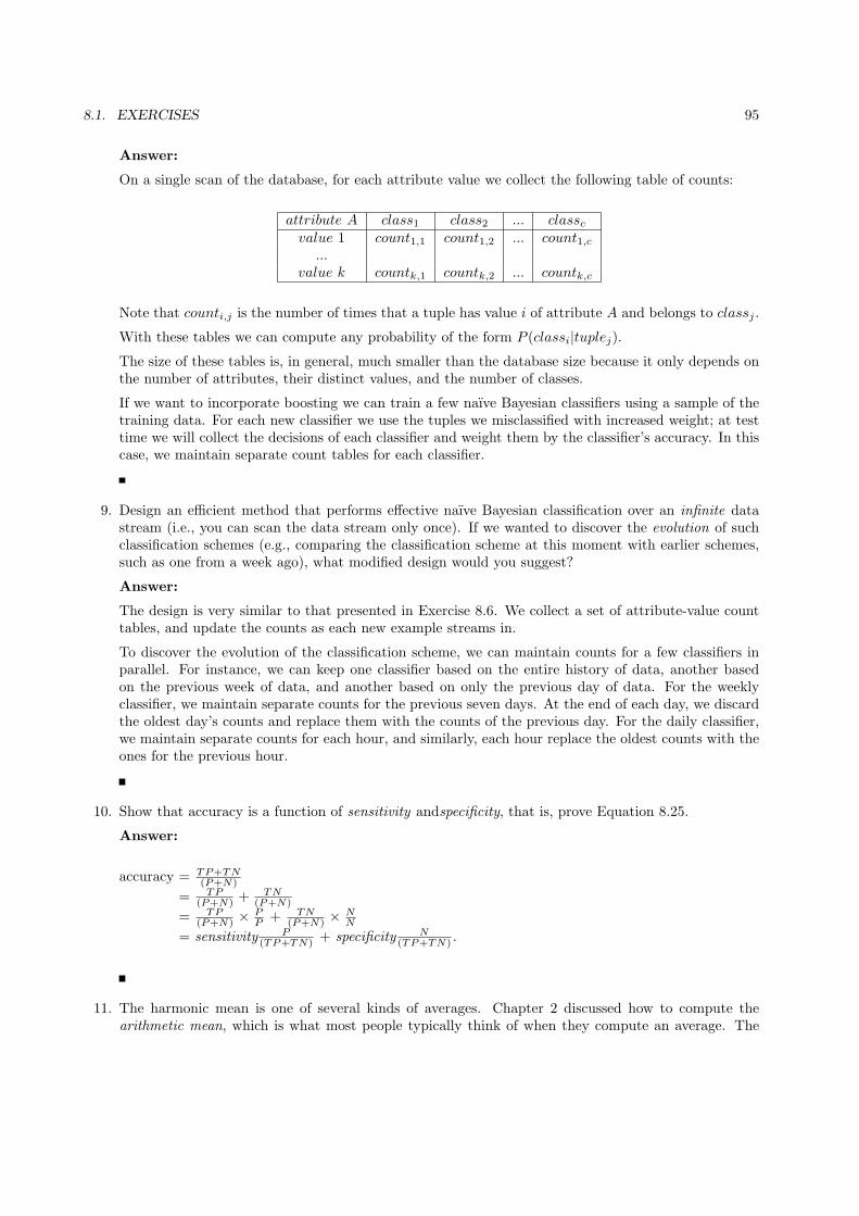
8.1. EXERCISES 95
Answer:
On a single scan of the database, for each attribute value we collect the following table of counts:
attribute A class1 class2 ... classcvalue 1 count1,1 count1,2 ... count1,c
...value k countk,1 countk,2 ... countk,c
Note that counti,j is the number of times that a tuple has value i of attribute A and belongs to classj .
With these tables we can compute any probability of the form P (classi|tuplej).The size of these tables is, in general, much smaller than the database size because it only depends onthe number of attributes, their distinct values, and the number of classes.
If we want to incorporate boosting we can train a few naıve Bayesian classifiers using a sample of thetraining data. For each new classifier we use the tuples we misclassified with increased weight; at testtime we will collect the decisions of each classifier and weight them by the classifier’s accuracy. In thiscase, we maintain separate count tables for each classifier.
9. Design an efficient method that performs effective naıve Bayesian classification over an infinite datastream (i.e., you can scan the data stream only once). If we wanted to discover the evolution of suchclassification schemes (e.g., comparing the classification scheme at this moment with earlier schemes,such as one from a week ago), what modified design would you suggest?
Answer:
The design is very similar to that presented in Exercise 8.6. We collect a set of attribute-value counttables, and update the counts as each new example streams in.
To discover the evolution of the classification scheme, we can maintain counts for a few classifiers inparallel. For instance, we can keep one classifier based on the entire history of data, another basedon the previous week of data, and another based on only the previous day of data. For the weeklyclassifier, we maintain separate counts for the previous seven days. At the end of each day, we discardthe oldest day’s counts and replace them with the counts of the previous day. For the daily classifier,we maintain separate counts for each hour, and similarly, each hour replace the oldest counts with theones for the previous hour.
10. Show that accuracy is a function of sensitivity andspecificity, that is, prove Equation 8.25.
Answer:
accuracy = TP+TN(P+N)
= TP(P+N) +
TN(P+N)
= TP(P+N) ×
PP + TN
(P+N) ×NN
= sensitivity P(TP+TN) + specificity N
(TP+TN) .
11. The harmonic mean is one of several kinds of averages. Chapter 2 discussed how to compute thearithmetic mean, which is what most people typically think of when they compute an average. The

96 CHAPTER 8. CLASSIFICATION: BASIC CONCEPTS
Tuple # Class Prob.
1 p 0.952 n 0.853 p 0.784 p 0.665 n 0.606 p 0.557 n 0.538 n 0.529 n 0.5110 p 0.4
Figure 8.1: Tuples sorted by decreasing score, where the score is the value returned by a probabilisticclassifier.
harmonic mean, H, of the positive real numbers, x1, x2, . . . , xn is defined as
H =n
1x1
+ 1x2
+ . . .+ 1xn
=n∑n
i=11xi
The F measure is the harmonic mean of precision and recall. Use this fact to derive Equation (8.28)for F . In addition, write Fβ as a function of true positives, false negatives, and false positives.
Answer:
F =2
1
precision+
1
recall
=2× precision× recall
precision+ recall
F beta =(1 + β2)× TP
(1 + β2)× TP + (β2 × FN) + FP
12. The data tuples of Figure 8.25 are sorted by decreasing probability value, as returned by a classifier.For each tuple, compute the values for the number of true positives (TP ), false positives (FP ), truenegatives (TN), and false negatives (FN). Compute the true positive rate (TPR) and false positiverate (FPR). Plot the ROC curve for the data.
Answer:
See Figure 8.2 and Figure 8.3
13. It is difficult to assess classification accuracy when individual data objects may belong to more thanone class at a time. In such cases, comment on what criteria you would use to compare differentclassifiers modeled after the same data.
Answer:

8.1. EXERCISES 97
Tuple # Class Prob. TP FP TN FN TPR FPR
1 p 0.95 1 0 5 4 0.2 02 n 0.85 1 1 4 4 0.2 0.23 p 0.78 2 1 4 3 0.4 0.24 p 0.66 3 1 4 2 0.6 0.25 n 0.60 3 2 3 2 0.6 0.46 p 0.55 4 2 3 1 0.8 0.47 n 0.53 4 3 2 1 0.8 0.68 n 0.52 4 4 1 1 0.8 0.89 n 0.51 4 5 0 1 0.8 110 p 0.4 5 5 0 0 1 0
Figure 8.2: TP, FP, TN, FN, TPR and FPR of the data of Excercise 8.12.
0 0.2 0.4 0.6 0.8 10
0.1
0.2
0.3
0.4
0.5
0.6
0.7
0.8
0.9
1
False positive rate (1−Specificity)
Tru
e po
sitiv
e ra
te (
Sen
sitiv
ity)
ROC curve
Figure 8.3: ROC curve of the data of Exercise 8.12.
A data object may belong to more than one class at a time. However, that data object will belongto some classes more often than other classes. Therefore, one criterion that can be used to assessclassification accuracy is to choose the classifier that predicts the class to which the data object usuallybelongs. Alternatively, a second-guess heuristic may be used, whereby a class prediction is judged ascorrect if it agrees with the first or second most probable class. Other criteria that may be used tocompare different classifiers modeled after the same data include speed, robustness, scalability, andinterpretability.
Generally, we prefer classifiers that minimize computational costs (e.g. training time, classificationtime), make accurate predictions even when given noisy data or incomplete data, work efficiently givenlarge amounts of data, and provide concise results that are easy to understand.
14. Suppose that we would like to select between two prediction models, M1 and M2. We have performed10 rounds of 10-fold cross validation on each model, where the same data partitioning in round i is

98 CHAPTER 8. CLASSIFICATION: BASIC CONCEPTS
used for both M1 and M2. The error rates obtained for M1 are 30.5, 32.2, 20.7, 20.6, 31.0, 41.0, 27.7,26.0, 21.5, 26.0. The error rates for M2 are 22.4, 14.5, 22.4, 19.6, 20.7, 20.4, 22.1, 19.4, 16.2, 35.0.Comment on whether one model is significantly better than the other considering a significance levelof 1%.
Answer:
We can do hypothesis testing to see if there is a significant difference in average error. Given that weused the same test data for each observation we can use the “paired observation” hypothesis test tocompare two means:
H0 : x1 − x2 = 0H1 : x1 − x2 = 0
Where x1 is the mean error of model M1, and x2 is the mean error of model M2.
We compute the test statistic t using the formula:
t =d
sd/√n
(8.1)
where d is the mean of the differences in error, sd is the standard deviation of the differences in error,and n is the number of observations. In this case d = 6.45, sd = 8.25, and n = 10. Replacing thisvalues in the equation we get t = 2.47. Using a t distribution table, we look tα/2 value for probability0.005 and 9 degrees of freedom, which is 3.25. Given that −3.25 < 2.47 < 3.25 we accept the nullhypothesis, i.e., the two models are not different at a significance level of 0.01.
15. What is boosting? State why it may improve the accuracy of decision tree induction.
Answer:
Boosting is a technique used to help improve classifier accuracy. We are given a set S of s tuples. Foriteration t, where t = 1, 2, . . . , T , a training set St is sampled with replacement from S. Assign weightsto the tuples within that training set. Create a classifier, Ct from St. After Ct is created, update theweights of the tuples so that the tuples causing classification error will have a a greater probability ofbeing selected for the next classifier constructed. The final boosting classifier combines the votes ofeach individual classifier, where the weight of each classifier’s vote is a function of its accuracy. Itcan be proved that with the number of weak classifiers increasing, the training error of combinationboosting classifier drops.
16. Outline methods for addressing the class imbalance problem. Suppose a bank would like to developa classifier that guards against fraudulent credit card transactions. Illustrate how you can induce aquality classifier based on a large set of non-fraudulent examples and a very small set of fraudulentcases.
Answer:
There are in total four general approaches for improving the classification accuracy of class-imbalanceddata like the fraudulent credit card transactions data.
The first one is oversampling, which works by resampling the positive tuples so that the resultingtraining set contains an equal number of positive and negative tuples. So for the data in the question,we can replicate tuples of the fraudulent cases to form a training set with size comparable to non-fraudulent examples.
The second one is undersampling, which works by decreasing the number of negative tuples. Itrandomly eliminates tuples from the majority (negative) class until there are an equal number of
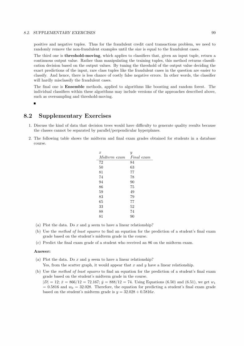
8.2. SUPPLEMENTARY EXERCISES 99
positive and negative tuples. Thus for the fraudulent credit card transactions problem, we need torandomly remove the non-fraudulent examples until the size is equal to the fraudulent cases.
The third one is threshold-moving, which applies to classifiers that, given an input tuple, return acontinuous output value. Rather than manipulating the training tuples, this method returns classifi-cation decision based on the output values. By tuning the threshold of the output value deciding theexact predictions of the input, rare class tuples like the fraudulent cases in the question are easier toclassify. And hence, there is less chance of costly false negative errors. In other words, the classifierwill hardly misclassify the fraudulent cases.
The final one is Ensemble methods, applied to algorithms like boosting and random forest. Theindividual classifiers within these algorithms may include versions of the approaches described above,such as oversampling and threshold-moving.
8.2 Supplementary Exercises
1. Discuss the kind of data that decision trees would have difficulty to generate quality results becausethe classes cannot be separated by parallel/perpendicular hyperplanes.
2. The following table shows the midterm and final exam grades obtained for students in a databasecourse.
x yMidterm exam Final exam72 8450 6381 7774 7894 9086 7559 4983 7965 7733 5288 7481 90
(a) Plot the data. Do x and y seem to have a linear relationship?
(b) Use the method of least squares to find an equation for the prediction of a student’s final examgrade based on the student’s midterm grade in the course.
(c) Predict the final exam grade of a student who received an 86 on the midterm exam.
Answer:
(a) Plot the data. Do x and y seem to have a linear relationship?
Yes, from the scatter graph, it would appear that x and y have a linear relationship.
(b) Use the method of least squares to find an equation for the prediction of a student’s final examgrade based on the student’s midterm grade in the course.
|D| = 12; x = 866/12 = 72.167; y = 888/12 = 74. Using Equations (6.50) and (6.51), we get w1
= 0.5816 and w0 = 32.028. Therefore, the equation for predicting a student’s final exam gradebased on the student’s midterm grade is y = 32.028 + 0.5816x.

100 CHAPTER 8. CLASSIFICATION: BASIC CONCEPTS
(c) Predict the final exam grade of a student who received an 86 on the midterm exam.
Using the formula from part (b), we get y = 32.028+ (0.5816)(86) = 82.045. Therefore, we wouldpredict that a student who received an 86 on the midterm would get 82 on the final exam.
3. Some nonlinear regression models can be converted to linear models by applying transformations tothe predictor variables. Show how the nonlinear regression equation y = αXβ can be converted to alinear regression equation solvable by the method of least squares.
Answer:
Apply the substitutions y′ = log(y), w′0 = log(w0), w
′1 = w1, x
′ = log(x), in order to obtain the linearmodel y′ = w′
0 + w′1x
′.

Chapter 9
Classification: Advanced Methods
9.1 Exercises
1. The following table consists of training data from an employee database. The data have been gener-alized. For example, “31 . . . 35” for age represents the age range of 31 to 35. For a given row entry,count represents the number of data tuples having the values for department, status, age, and salarygiven in that row.
department status age salary countsales senior 31. . . 35 46K. . . 50K 30sales junior 26. . . 30 26K. . . 30K 40sales junior 31. . . 35 31K. . . 35K 40systems junior 21. . . 25 46K. . . 50K 20systems senior 31. . . 35 66K. . . 70K 5systems junior 26. . . 30 46K. . . 50K 3systems senior 41. . . 45 66K. . . 70K 3marketing senior 36. . . 40 46K. . . 50K 10marketing junior 31. . . 35 41K. . . 45K 4secretary senior 46. . . 50 36K. . . 40K 4secretary junior 26. . . 30 26K. . . 30K 6
Let status be the class label attribute.
(a) Design a multilayer feed-forward neural network for the given data. Label the nodes in the inputand output layers.
(b) Using the multilayer feed-forward neural network obtained above, show the weight values after oneiteration of the backpropagation algorithm, given the training instance “(sales, senior, 31. . . 35,46K. . . 50K)”. Indicate your initial weight values and biases, and the learning rate used.
Answer:
(a) There is no standard answer. Every feasible solution is correct. As stated in the book, discrete-valued attributes may be encoded such that there is one input unit per domain value. For hiddenlayer units, the number should be smaller than that of input units, but larger than that of outputunits.
(b) There is no standard answer. Every feasible solution is correct.
101
102 CHAPTER 9. CLASSIFICATION: ADVANCED METHODS
2. The support vector machine (SVM) is a highly accurate classification method. However, SVM classifierssuffer from slow processing when training with a large set of data tuples. Discuss how to overcome thisdifficulty and develop a scalable SVM algorithm for efficient SVM classification in large datasets.
Answer:
We can use the micro-clustering technique in “Classifying large data sets using SVM with hierarchicalclusters” by Yu, Yang, and Han, in Proc. 2003 ACM SIGKDD Int. Conf. Knowledge Discovery andData Mining (KDD’03), pages 306-315, Aug. 2003 [YYH03]. A Cluster-Based SVM (CB-SVM)method is described as follows:
1. Construct the microclusters using a CF-Tree (Chapter 7).
2. Train an SVM on the centroids of the microclusters.
3. Decluster entries near the boundary.
4. Repeat the SVM training with the additional entries.
5. Repeat the above until convergence.
3. Compare and contrast associative classification and discriminative frequent pattern-based classification.Why is classification based on frequent patterns able to achieve higher classification accuracy in manycases than a classical decision-tree method?
Answer:
Association-based classification is a method where association rules are generated and analyzed foruse in classification. We first search for strong associations between frequent patterns (conjunctions ofattribute-value pairs) and class labels. Using such strong associations we classify new examples.
Discriminative frequent pattern-based classification first finds discriminative frequent patterns accord-ing to certain measures such as pattern length and pattern frequency and uses these patterns asfeatures. Then it trains classifiers based on these features.
Frequent pattern-based classification can achieve higher accuracy than a classical decision tree becauseit overcomes the constraint of decision trees, which consider only one attribute at a time. Some frequentpatterns could have very high discriminative power because they combine multiple attributes.
4. Compare the advantages and disadvantages of eager classification (e.g., decision tree, Bayesian, neuralnetwork) versus lazy classification (e.g., k-nearest neighbor, case-based reasoning).
Answer:
Eager classification is faster at classification than lazy classification because it constructs a general-ization model before receiving any new tuples to classify. Weights can be assigned to attributes, whichcan improve classification accuracy. Disadvantages of eager classification are that it must commit toa single hypothesis that covers the entire instance space, which can decrease classification, and moretime is needed for training.
Lazy classification uses a richer hypothesis space, which can improve classification accuracy. Itrequires less time for training than eager classification. A disadvantages of lazy classification is that alltraining tuples need to be stored, which leads to expensive storage costs and requires efficient indexingtechniques. Another disadvantage is that it is slower at classification because classifiers are not builtuntil new tuples need to be classified. Furthermore, attributes are all equally weighted, which candecrease classification accuracy. (Problems may arise due to irrelevant attributes in the data.)

9.1. EXERCISES 103
Algorithm: k-nearest neighbor. Build a k-nearest neighbor classifier.
Input:
• Let U be the unknown tuple whose class we want to assign.
• Let T be the training set containing training tuples, T1 = (t1,1, t1,2, . . . , t1,n), T2 = (t2,1, t2,2, . . . , t2,n), . . . , Tm =(tm,1, tm,2, . . . , tm,n).
• Let attribute ti,n be the class label of Ti.
• Let m be the number of training tuples.
• Let n be the number of attributes describing each tuple.
• Let k be the number of nearest neighbors we wish to find.
Output: Class label for U .
Method: The method is outlined as follows.
1) array a[m][2]; // m rows containing data regarding the m training tuples. The first column is theEuclidean distance between U and that row’s training tuple. The second column refers to thattraining tuple’s index. We need to save the index because when sorting the array (according toEuclidean distance), we need some way to determine to which training set the Euclidean distance refers.
2) for i = 1 to m do {3) a[i][1] = Euclidean distance(U, Ti);4) a[i][2] = i;} // save the index, because rows will be sorted later5) Sort the rows of a by their Euclidean distances saved in a[i][1] (in ascending order);6) array b[k][2]; // The first column holds the distinct class labels of the k-nearest neighbors, while the
second holds their respective counts. In the worst case, each k-nearest neighbor will have a differentclass label, which is why we need to allocate room for k class labels.
7) for i = 1 to k do {8) if class label ta[i][2],n already exists in array b then9) find that class label’s row in array b and increment its count;10) else add the class label into the next available row of array b and increment its count; }11) Sort array b in descending order (from class label with largest count down to that with smallest count);12) return(b[1]); //return most frequent class label of the k-nearest neighbors of U as the class prediction.
Figure 9.1: k-nearest neighbor algorithm.
5. Write an algorithm for k-nearest neighbor classification given k, the nearest number of neighbors, andn, the number of attributes describing each tuple.
Answer:
Figure 9.1 presents an algorithm for k-nearest neighbor classification.
6. Briefly describe the classification processes using i) genetic algorithms, ii) rough sets, and iii) fuzzysets.
Answer:
i) Genetic algorithms is based on an analogy to biological evolution.
• An initial population is created consisting of randomly generated rules. Each rule is repre-sented by a string of bits. If an attribute has k > 2 values, k bits can be used.
• Based on the notion of survival of the fittest, a new population is formed to consist of the fittestrules and their offspring. The fitness of a rule is represented by its classification accuracy ona set of training examples.
• Offspring are generated by crossover and mutation.
The process continues until a population P evolves when each rule in P satisfies a prespecifiedthreshold.
ii) Rough sets are used to approximately or roughly define equivalent classes. A rough set for a givenclass C is approximated by two sets: a lower approximation (certain to be in C) and an upperapproximation (cannot be described as not belonging to C).

104 CHAPTER 9. CLASSIFICATION: ADVANCED METHODS
iii) Fuzzy logic uses truth values between 0.0 and 1.0 to represent the degree of membership (such asin a fuzzy membership graph). Attribute values are converted to fuzzy values. Each applicablerule contributes a vote for membership in the categories. Typically, the truth values for eachpredicted category are summed, and these sums are combined.
7. Example 9.3 showed an example of the use of error-correcting codes for a multiclass classificationproblem having four classes.
(a) Suppose that, given an unknown tuple to label, the seven trained binary classifiers collectivelyoutput the codeword 0101110, which does not match a codeword for any of the four classes. Usingerror correction, what class label should be assigned to the tuple?
(b) Explain why using a 4-bit vector for the codewords is insufficient for error correction.
Answer:
(a) It should be assigned to C4, given it has the smallest Hamming distance 1.
(b) Since we want to do 4-class classification with error-correcting code, at least we should be able tocorrect 1-bit error. This requires the minimum hamming distance h between codewords to satisfy⌊h−1
2 ⌋ > 1, which means h > 3. Using 4-bit vector for a codeword, it is obvious that we cannotfind 4 4-bit vectors with minimum hamming distance 3 between any two of them. Therefore, it isinsufficient for error correction.
8. Semi-supervised classification, active learning and transfer learning are useful for situations in whichunlabeled data are abundant.
(a) Describe semi-supervised classification, active learning and transfer learning. Elaborate on appli-cations for which they are useful, as well as the challenges of these approaches to classification.
(b) Research and describe an approach to semi-supervised classification other than self-training andco-training.
(c) Research and describe an approach to active learning other than pool-based learning.
(d) Research and describe an alternative approach to instance-based transfer learning.
Answer:
(a) • Semi-supervised classification uses both labeled and unlabeled data to build a classifier.It is often used in the situation where unlabeled data are plentiful.Applications include intruder detection in a battlefield sensor network because it is costlyand error-prone to manually label the large sensor dataset. Semi-supervised leaarning isalso widely used in text classification.The main challenge for semi-supervised learning is how to find discriminative features toclassify the data.
• Active learning purposefully queries a user (e.g., a human oracle) for labels. And then ituses all the labelled data to train the classifier in a standard supervised way.Active learning is suitable for situations where data are abundant, yet the class labelsare scarce or expensive to obtain. It can be applied to the areas of text classification andimage retrieval and outperforms regular passive learning substantially.The main challenge for active learning is how to choose the data tuples to be queried.This can be computational expensive.

9.2. SUPPLEMENTARY EXERCISES 105
• Transfer Learning extracts knowledge from one or more source tasks and then apply theknowledge to a target task.Transfer learning is useful for applications where the data becomes outdated or the dis-tribution changes. Typical applications include web-document classification and emailspam filtering.The main challenge for transfer learning is negative transfer. This occurs when the newclassifier performs worse than if there had been no transfer at all.
(b) There are no standard answers to this question. An alternative approach is to model thejoint probability distribution of the features and the labels. For the unlabeled data the labelscan then be treated as ’missing data’. Techniques that handle missing data, such as Gibbssampling or the EM algorithm, can then be used to estimate the parameters of the model.
(c) There are no standard answers to this question. Alternative approaches could include mem-bership query synthesis and stream-based selective sampling.
• In the setting of membership query synthesis, the learner may request labels for anyunlabeled instance in the input space, including (and typically assuming) queries thatthe learner generates de novo, rather than those sampled from some underlying naturaldistribution. Efficient query synthesis is often tractable and efficient for finite problemdomains [1].
• In the setting of stream-based selective sampling, the key assumption is that obtainingan unlabeled instance is free (or inexpensive), so it can first be sampled from the actualdistribution, and then the learner can decide whether or not to request its label. Thisapproach is sometimes called stream-based or sequential active learning, as each unlabeledinstance is typically drawn one at a time from the data source, and the learner must decidewhether to query or discard it[1].
(d) There are no standard answers to this question. An alternative approach could be featurerepresentation-transfer. This approach aims at finding “good” feature representations tominimize domain divergence and classification or regression model error. Strategies to find“good” feature representations are different for different types of the source domain data. If alot of labeled data in the source domain are available, supervised learning methods can be usedto construct a feature representation. If no labeled data in the source domain are available,unsupervised learning methods are proposed to construct the feature representation[2].
[1] B. Settles. Active Learning Literature Survey. Computer Sciences Tech. Report 1648, Univ.of Wisconsin-Madison. 2009.
[2] S. J. Pan and Q. Yang, A Survey on Transfer Learning, IEEE Trans. on Knowledge and DataEngineering, 22(10):1345-1359, 2010.
9.2 Supplementary Exercises
1. To be added

106 CHAPTER 9. CLASSIFICATION: ADVANCED METHODS

Chapter 10
Cluster Analysis: Basic Concepts andMethods
10.1 Exercises
1. Briefly describe and give examples of each of the following approaches to clustering: partitioningmethods, hierarchical methods, density-based methods and grid-based methods.
Answer:
Clustering is the process of grouping data into classes, or clusters, so that objects within a clusterhave high similarity in comparison to one another, but are very dissimilar to objects in other clusters.There are several approaches to clustering methods.
Partitioning methods: Given a databases of n objects or data tuples, a partitioning methods con-structs k partitions of data, where each partition represents a cluster and k ≤ n. Given k, the numberof partitions to construct, it creates an initial partitioning. It then uses an iterative relocation tech-nique that attempts to improve the partitioning by moving objects from one group to another. Thegeneral criterion of a good partitioning is that objects in the same cluster are “close” or related to eachother, whereas objects of different clusters are “far apart”. For example, the k-means method is oneof the partitioning methods commonly used.
Hierarchical methods: A hierarchical method creates a hierarchical decomposition of the given setof data objects. It can be either agglomerative or divisive. The agglomerative (bottom-up) approachstarts with each object forming a separate group. It successively merges the objects close to one another,until all of the groups are merged into one, or until a termination condition holds. The divisive (top-down) approach starts with all objects in the same cluster. In each successive iteration, a cluster is splitup into smaller clusters, until eventually each object is in one cluster or until a termination conditionholds. BIRCH is an example of integration of hierarchical method with distance-based clustering.
Density-based methods: This method is based on density such as density-connected points. Themain idea is to continue growing a given cluster as long as the density in its “neighborhood” exceedssome threshold. That is, for each data point within a given cluster, the neighborhood of a given radiushas to contain at least a minimum number of points. This method can be used to filter out noise anddiscover clusters of arbitrary shape. DBSCAN is a typical example of density-based clustering method.
Grid-based methods: Such methods quantize the object space into a finite number of cells thatform a grid structure. All of the clustering operations are performed on the grid structure. The mainadvantage of this approach is its fast processing time, which is typically independent of the numberof data objects and dependent only on the number of cells in each dimension in the quantized space.STING is an example of a grid-based method.
107
108 CHAPTER 10. CLUSTER ANALYSIS: BASIC CONCEPTS AND METHODS
Model-based methods: This approach hypothesizes a model for each of the clusters and finds thebest fit of the data to the given model. It locates the clusters by constructing a density function thatreflects the spatial distribution of the data points. It also leads to a way of automatically determiningthe number of clusters based on standard statistics, taking “noise” or outliers into account and thusyielding robust clustering methods. COBWEB is an example of a statistical approach of a model-basedmethod.
2. Suppose that the data mining task is to cluster points (with (x, y) representing location) into threeclusters, where the points are
A1(2, 10), A2(2, 5), A3(8, 4), B1(5, 8), B2(7, 5), B3(6, 4), C1(1, 2), C2(4, 9).
The distance function is Euclidean distance. Suppose initially we assign A1, B1, and C1 as the centerof each cluster, respectively. Use the k-means algorithm to show only
(a) the three cluster centers after the first round of execution.
Answer:
After the first round, the three new clusters are: (1) {A1}, (2) {B1, A3, B2, B3, C2}, (3) {C1, A2},and their centers are (1) (2, 10), (2) (6, 6), (3) (1.5, 3.5).
(b) the final three clusters.
Answer:
The final three clusters are: (1) {A1, C2, B1}, (2) {A3, B2, B3}, (3) {C1, A2}.
3. Use an example to show why the k-means algorithm may not find the global optimum, that is, opti-mizing the within-cluster variation.
Answer:
Consider applying the k-means algorithm on the following points, and set k = 2. A(0, 1), B(0,−1),Ci(100, 50) (i = 1, . . . , 100), and Dj(100,−50) (j = 1, . . . , 100).
If we use A and C1 as the initial cluster centers, then the clustering process will converge to two centers,(0, 0) and (100, 0). The within-cluster variation is
E = 12 + 12 + 100× 502 + 100× 502 = 1 + 1 + 100× 2500 + 100× 2500 = 500002.
However, if we use (100, 50) and (100,−50) as the cluster centers, the within-cluster variation is
E = (1002 + 492) + (1002 + 492) + 100× 0 + 100× 0 = 24802,
which is much smaller. This example shows k-means may be trapped by a local optimal, and cannotjump out to find the global optimum.
4. For the k-means algorithm, it is interesting to note that by choosing the initial cluster centers carefully,we may be able to not only speed up the convergence of the algorithm, but also guarantee the qualityof the final clustering. The k-means++ algorithm is a variant of k-means, which chooses the initialcenters as follows. First, it selects one center uniformly at random from the objects in the data set.Iteratively, for each object p other than the chosen center, it chooses an object as the new center. Thisobject is chosen at random with probability proportional to dist(p)2, where dist(p)) is the distance

10.1. EXERCISES 109
from p) to the closest center that has already been chosen. The iteration continues until k centers areselected.
Explain why this method will not only speed up the convergence of the k-means algorithm, but alsoguarantee the quality of the final clustering results.
Answer:
Please refer to [AV07].
5. Provide the pseudo-code of the object re-assignment step of the PAM algorithm.
Answer:
Let o1, . . . , ok be the current medoids. Suppose we are considering to use object orandom to replacemedoid object oi (1 ≤ i ≤ k). Then, we need to reassign all the other objects in the data set. Thepseudo-code of the re-assignment step is as follows.
1: for each object o assigned to oj (1 ≤ j ≤ k, j = i) do2: if dist(o, oj) > dist(o, orandom) then3: assign o to orandom4: else5: still assign o to oj6: end if7: end for8: for each object o assigned to oi, including oi do9: j = argmin1≤l≤k,l =i{dist(o, ol)}
10: if dist(o, orandom) < dist(o, oj) then11: assign o to orandom12: else13: assign o to oj14: end if15: end for
6. Both k-means and k-medoids algorithms can perform effective clustering.
(a) Illustrate the strength and weakness of k-means in comparison with the k-medoids algorithm.
Answer:
k-means vs. k medoids: more efficient but quality deteriorates by noise and outliers.
(b) Illustrate the strength and weakness of these schemes in comparison with a hierarchical clusteringscheme (such as AGNES).
Answer:
Partition: can undo what was done (by moving objects around clusters)—quality is good ingeneral, require the number of clusters to be known; find only spherical shaped clusters.
Hierarchical: cannot undo what was done—quality could be poor, does not require the numberof clusters to be known; more efficient and parallel (divide and conquer), may find only arbitraryshaped clusters.
7. Prove that in DBSCAN, the density-connectedness is an equivalence relation.
Answer:
110 CHAPTER 10. CLUSTER ANALYSIS: BASIC CONCEPTS AND METHODS
Given a radius of neighborhood ϵ > 0 and a density threshold MinPts > 0, DBSCAN partitions a setof objects into density-based clusters. We show that the density-connectedness used in DBSCAN is anequivalence relation on the set of objects O, where for any object o ∈ O, o belongs to a cluster.
Reflexivity For any object o ∈ O, since o belongs to a cluster, there must be an o′ ∈ O such thato and o′ are density-connected. Applying the definition of density-connectedness, trivially o anditself are density-connected.
Symmetry Recall that two objects o1, o2 ∈ O are density-connected with respect to ϵ and MinPts,if there is an object o ∈ O such that both o1 and o2 are density-reachable from o with respect toϵ and MinPts. The symmetry follows with the definition immediately.
Transitivity According to DBSCAN, all core objects in a cluster are density-reachable from eachother. The set of objects inserted into N in the algorithm when a cluster is explored justifies thedensity-reachability of the core objects.
Suppose o1 and o2 are density-connected, and so are o2 and o3, determined by DBSCAN. Then,there are core objects o′ and o′′ such that o1 and o2 are density-reachable from o′ and o2 and o3 aredensity-reachable from o′′. Moreover, o′ and o′′ must be assigned to the same density-based clusterby DBSCAN. Otherwise, DBSCAN does not explore the density-connectedness between o1 ando2 and that between o2 and o3 at the same time. Therefore, both o1 and o3 are density-reachablefrom o′ (and o′′ as well). That is, o1 and o3 are density-connected.
Please note that, in general, the density-connectedness is NOT an equivalence relation. It is possiblethat an object o, which is not a core object, is directly density-reachable from two core objects o1 ando2 that belong to two different clusters. In such a case, DBSCAN arbitrarily assigns o to one cluster,say the cluster containing o1, and does not regard o is density-reachable from o2.
8. Prove that in DBSCAN, for a fixed MinPts value and two neighborhood thresholds ϵ1 < ϵ2, a clusterC with respect to ϵ1 and MinPts must be a subset of a cluster C ′ with respect to ϵ2 and MinPts.
Answer:
For any core object q and object p such that p is directly density-reachable from q with respect to ϵ1,q is also directly density-reachable from q with respect to ϵ2. Thus, if an object p is density-reachablefrom object q with respect to ϵ1, p is still density-reachable from q with respect to ϵ2. Therefore, ifobjects p and q are density-connected with respect to ϵ1, they are density-connected with respect toϵ2. Consequently, all objects in cluster C with respect to ϵ1 must be grouped into a cluster C ′ withrespect to ϵ2.
9. Provide the pseudo-code of the OPTICS algorithm.
Answer:
Please refer to Figures 5-8 in [ABKS99].
10. Why is it that BIRCH encounters difficulties in finding clusters of arbitrary shape but OPTICS doesnot? Can you propose some modifications to BIRCH to help it find clusters of arbitrary shape?
Answer:
BIRCH uses Euclidean distance and inter-cluster proximity as distance measure, which leads to spher-ical shaped clusters.
OPTICS uses density-based (connectivity) measure, which grows clusters based on the connected pointswithin a defined radius, and thus can find arbitrary shaped clusters.

10.1. EXERCISES 111
There could be several ways to modify BIRCH. One is to use density-based and connectivity-based dis-tance measure to cluster low-level B+-trees and build levels of CF-tree which will lead to connectivity-based (arbitrary-shaped) cluster.
11. Provide the pseudo-code of the step in CLIQUE finding dense cells in all subspaces.
Answer:
Please refer to Section 3.1.1 in [AGGR98].
12. Present conditions under which density-based clustering is more suitable than partitioning-based clus-tering and hierarchical clustering. Give application examples to support your argument.
Answer:
Density-based clustering is more suitable if no or very limited domain knowledge is available to de-termine the appropriate values of the parameters, the clusters are expect of arbitrary shape includingnon convex shapes, and the efficiency is essential on large data sets.
For example, consider the application of recognizing residential area on a map where buildings andtheir types are labeled. A user may not have the domain knowledge about how a residential area wouldlook like. Moreover, a residential area may be of arbitrary shape, and may not be in convex, such asthose built along a river. In a large city, there are hundreds of thousands of buildings. Efficiency onlarge data sets is important.
13. Give an example of how specific clustering methods can be integrated, for example, where one clusteringalgorithm is used as a preprocessing step for another. In addition, provide reasoning as to why theintegration of two methods may sometimes lead to improved clustering quality and efficiency.
Answer:
Consider building an ontology of queries for information retrieval and web search. A query is associatedwith a vector of web pages that are clicked when the query is asked. An effective approach is to firstconduct density-based clustering to form small clusters as micro-clusters. Each micro-cluster is treatedas a base unit, sometimes called a concept. Then, a hierarchical clustering method can be applied tobuild an ontology.
To use density-based clustering as a pre-processing step can quickly merge synonyms, such as “Uni-versity of Illinois at Urbana-Champaign” and “UIUC”, into one concept. This preprocessing step canreduce the data so that the ontology built later is more meaningful, and the ontology building processis faster.
14. Clustering is recognized as an important data mining task with broad applications. Give one applicationexample for each of the following cases:
(a) An application that takes clustering as a major data mining function
Answer:
For example, clustering is a major data mining function in community finding in social networks.
(b) An application that takes clustering as a preprocessing tool for data preparation for other datamining tasks.
Answer:

112 CHAPTER 10. CLUSTER ANALYSIS: BASIC CONCEPTS AND METHODS
Web search engines often provide query suggestion services. When a user inputs one or a series ofqueries, the search engine tries to suggest some queries that may capture the user’s informationneed. To overcome the data sparsity, that is, many queries are asked very few times, and manyweb pages are not clicked, clustering is often used as a preprocessing step to obtain micro-clustersof queries, which represent similar user intents, and web pages, which are about the same topics.
15. Data cubes and multidimensional databases contain categorical, ordinal, and numerical data in hier-archical or aggregate forms. Based on what you have learned about the clustering methods, design aclustering method that finds clusters in large data cubes effectively and efficiently.
Answer:
For example, CLIQUE can be extended to a data cube.
16. Describe each of the following clustering algorithms in terms of the following criteria: (1) shapes ofclusters that can be determined; (2) input parameters that must be specified; and (3) limitations.
(a) k-means
(b) k-medoids
(c) CLARA
(d) BIRCH
(e) CHAMELEON
(f) DBSCAN
Answer:
(a) k-means
1. Compact clouds (clusters of non-convex shape cannot be determined); 2. Number of clusters;3. Sensitive to noise and outliers, works good on small data sets only.
(b) k-medoids
1. Compact clouds (clusters of non-convex shape cannot be determined); 2. Number of clusters;3. Small data sets (not scalable).
(c) CLARA
1. Convex-shaped clusters; 2. Number of clusters; 3. Sensitive to the selection of initial samples.
(d) BIRCH
1. Spherical in shape clusters; 2. N d-dimensional data points; 3. Resulting clusters may be ofunnatural shape.
(e) CHAMELEON
1. Arbitrary shape; 2. N d-dimensional categorical points; 3. Quadratic time in the worst case.
(f) DBSCAN
1. Arbitrary shape; 2. Maximum possible distance for a point to be considered density reachableand minimum number of points in a cluster. 3. Quadratic time in the worst case.
17. Human eyes are fast and effective at judging the quality of clustering methods for 2-D data. Canyou design a data visualization method that may help humans visualize data clusters and judge theclustering quality for 3-D data? What about for even higher-dimensional data?

10.1. EXERCISES 113
Answer:
One method is as follows: We first use a clustering algorithm to obtain clusters from the three-dimensional data. We then paint the clusters found. These can be “projected” onto two-dimensionaldata to obtain the clusters in the 2-D space, making it easier for humans to visualize. To help gaingreater insight as to the quality of clusters for the 3-D data, we can then rotate the data space atdifferent angles. Later, we can project onto another set of 2-D data, to similarly rotate the data space.By comparing the different 2-D space clusters, we have a better idea of the clusters in the 3-D data.
For higher dimensional data we can use a method of coloring. First we transform the higher dimensionaldata into lower dimensional data and then use an arbitrary clustering algorithm to obtain the clustersat this lower level. We then paint the clusters into different colors, and continuously perform clusteringon the higher dimensional data. Ideally, we gain greater insight as to the quality of the clusters bycomparing the colors of the clusters.
18. Suppose that you are to allocate a number of automatic teller machines (ATMs) in a given region soas to satisfy a number of constraints. Households or places of work may be clustered so that typicallyone ATM is assigned per cluster. The clustering, however, may be constrained by two factors: (1)obstacle objects, i.e., there are bridges, rivers, and highways that can affect ATM accessibility, and (2)additional user-specified constraints, such as each ATM should serve at least 10,000 households. Howcan a clustering algorithm such as k-means be modified for quality clustering under both constraints?
Answer:
Constraint algorithms can be modified in the following aspects to allow for constraint-based clusteringas specified in the exercise. (We list only some examples):
• Micro-cluster. Objects are clustered locally into micro-clusters. In a micro-cluster, no obstaclecan appear between any two other objects in the micro-cluster.
• Distance measurement. Distance between two objects should be adjusted if obstacles occurbetween them. In such cases, reachable distance, instead of direct distance, should be used.Reachable distance gives the minimal (or estimated minimal) distance between two objects withconsideration of obstacles.
• Medoid-based. For every district, initialize k clusters, where k is between the minimum andmaximum number of ATMs allowed in the district. When a medoid is going to be moved acrossa district border, if after such a move the source district has fewer ATMs than required, or thedestination district has more ATMs than expected, then the center can only be moved within theborder to the point closest to the corresponding point in the other region.
19. For constraint-based clustering, aside from having the minimum number of customers in each cluster(for ATM allocation) as a constraint, there could be many other kinds of constraints. For example, aconstraint could be in the form of the maximum number of customers per cluster, average income ofcustomers per cluster, maximum distance between every two clusters, and so on. Categorize the kindsof constraints that can be imposed on the clusters produced and discuss how to perform clusteringefficiently under such kinds of constraints.
Answer:
Pleaser refer to [THH01].
114 CHAPTER 10. CLUSTER ANALYSIS: BASIC CONCEPTS AND METHODS
20. Design a privacy-preserving clustering method so that a data owner would be able to ask a third partyto mine the data for quality clustering without worrying about the potential inappropriate disclosureof certain private or sensitive information stored in the data.
Answer:
Please refer to, for example, [VC03, AY08].
21. Show that BCubed metrics satisfy the four essential requirements for extrinsic clustering evaluationmethods.
Answer:
Cluster homogeneity Consider clustering C1, wherein a cluster C ∈ C1 contains objects from twocategories L1, L2 in the ground truth. Moreover, consider clustering C2, which is identical to C1except that C is split into two clusters containing objects in L1 and L2, respectively. Let C1(o)and C2(o) be the cluster-id of o in C1 and C2, respectively.The BCubed precision of C1 is
Prec(C1) =∑
o ∈C
∑o′ =o,C1(o)=C1(o′)Correctness(o,o
′)
∥{o′ =o|C1(o)=C1(o′)}∥ +∑
o∈C
∑o′ =o,C1(o)=C1(o′)Correctness(o,o
′)
∥{o′ =o|C1(o)=C1(o′)}∥
total number of objects in the data set
The BCubed precision of C2 is
Prec(C2) =∑
o ∈C
∑o′ =o,C2(o)=C2(o′)Correctness(o,o
′)
∥{o′ =o|C2(o)=C2(o′)}∥ +∑
o∈C
∑o′ =o,C2(o)=C2(o′)Correctness(o,o
′)
∥{o′ =o|C2(o)=C2(o′)}∥
total number of objects in the data set
Since C1 and C2 are identical except for cluster C, we have
∑o∈C
∑o′ =o,C1(o)=C1(o′)
Correctness(o, o′)
∥{o′ = o|C1(o) = C1(o′)}∥=
∑o ∈C
∑o′ =o,C2(o)=C2(o′)
Correctness(o, o′)
∥{o′ = o|C2(o) = C2(o′)}∥
In C1, C is a mixture of the objects from two categories L1 and L2. In C2, C is divided into twoclusters containing the objects in the two categories respectively. Therefore,
∑o∈C
∑o′ =o,C1(o)=C1(o′)
Correctness(o, o′)
∥{o′ = o|C1(o) = C1(o′)}∥<
∑o∈C
∑o′ =o,C2(o)=C2(o′)
Correctness(o, o′)
∥{o′ = o|C2(o) = C2(o′)}∥
Thus, we have Prec(C1) < Prec(C2). Similarly, we can show Recall(C1) < Recall(C2).
Cluster completeness The proof of the cluster completeness is similar to that of the cluster homo-geneity.
Rag bag Consider a clustering C1 and a cluster C ∈ C1 such that all objects in C except for one,denoted by o, belong to the same category according to the ground truth. Consider a clusteringC2 identical to C1 except that o is assigned to a cluster C ′ = C in C2 such that C ′ contains objectsfrom various categories according to the ground truth. In other words, C ′ ∈ C2 is a rag bag. Weshow that the BCubed precision of C2 is greater than that of C1.In the BCubed precision calculation, Prec(C1) and Prec(C2) are the same except for those objectpairs involving o.

10.2. SUPPLEMENTARY EXERCISES 115
Prec(C2)− Prec(C1) = [(∥C ′∥ − 1)1
∥C ′∥ − 1+
number of objects in C ′ in the same category of o
∥C ′∥ − 1
−(∥C∥ − 1)1
∥C∥ − 1]/total number of objects in the data set
=number of objects in C ′ in the same category of o
(∥C ′∥ − 1)× total number of objects in the data set
≥ 0
In the worst case, there is no object in C ′ that is in the same category of o, Prec(C2)−Prec(C1) = 0.As long as there is at least one object in C ′ that is in the same category of o, Prec(C2)−Prec(C1) >0.
The BCubed recall can be analyzed in a similar way.
Small cluster preservation Suppose there are two categories, L1 and L2, in the ground truth suchthat ∥L1∥ > ∥L2∥. Consider a clustering C1 wherein the objects in L1 are divided into two clustersC11 and C12, and the objects in L2 are contained in a cluster C2. Consider a clustering C2 identicalto C1 except that C11 and C12 are merged into one cluster C1 and the objects in L2 are dividedinto two clusters C21 and C22. It is easy to verify that Rec(C2) > Rec(C1).
10.2 Supplementary Exercises
1. Briefly outline how to compute the dissimilarity between objects described by the following types ofvariables:
(a) Asymmetric binary variables
Answer: If all binary variables have the same weight, we have the contingency Table 10.1. Use
object j1 0 sum
1 q r q + robject i 0 s t s+ t
sum q + s r + t p
Table 10.1: A contingency table for binary variables.
the Jaccard coefficient, where the number of negative matches, t, is considered unimportant andthus is ignored in the computation, that is,
d(i, j) =r + s
q + r + s(10.1)
(b) Nominal variables
Answer: A nominal variable is a generalization of the binary variable in that it can take onmore than two states.
The dissimilarity between two objects i and j can be computed using the simple matchingapproach as in (10.2):
d(i, j) =p−m
p, (10.2)

116 CHAPTER 10. CLUSTER ANALYSIS: BASIC CONCEPTS AND METHODS
where m is the number of matches (i.e., the number of variables for which i and j are in the samestate), and p is the total number of variables.
Alternatively, we can use a large number of binary variables by creating a new binary variablefor each of the M nominal states. For an object with a given state value, the binary variablerepresenting that state is set to 1, while the remaining binary variables are set to 0.
(c) Ratio-scaled variables
Answer: Three methods include:
• Treat ratio-scaled variables as interval-scaled variables, so that the Minkowski, Manhattan,or Euclidean distance can be used to compute the dissimilarity.
• Apply a logarithmic transformation to a ratio-scaled variable f having value xif for object iby using the formula yif = log(xif ). The yif values can be treated as interval-valued,
• Treat xif as continuous ordinal data, and treat their ranks as interval-scaled variables.
(d) Numerical (interval-scaled) variables
Answer: Use Euclidean distance or Manhattan distance. Euclidean distance is defined as
d(i, j) =√|xi1 − xj1|2 + |xi2 − xj2|2 + · · ·+ |xip − xjp|2. (10.3)
where i = (xi1, xi2, . . . , xip), and j = (xj1, xj2, . . . , xjp), are two p-dimensional data objects.
The Manhattan (or city block) distance, is defined as
d(i, j) = |xi1 − xj1|+ |xi2 − xj2|+ · · ·+ |xip − xjp|. (10.4)
2. Given the following measurements for the variable age:
18, 22, 25, 42, 28, 43, 33, 35, 56, 28,
standardize the variable by the following:
(a) Compute the mean absolute deviation of age.
Answer: The mean absolute deviation of age is 8.8, which is derived as follows.
mf =1
n(x1f + · · ·+ xnf ) =
1
10(18 + 22 + 25 + 42 + 28 + 43 + 33 + 35 + 56 + 28) = 33
sf =1
n(|x1f −mf |+ · · ·+ |xnf −mf |)
=1
10(|18− 33|+ |22− 33|+ |25− 33|+ |42− 33|+ |28− 33|+ |43− 33|+ |33− 33|+ |35− 33|
+|56− 33|+ |28− 33|)= 8.8
(b) Compute the z-score for the first four measurements.
Answer: According to the z-score computation formula,
zif =xif −mif
sf. (10.5)
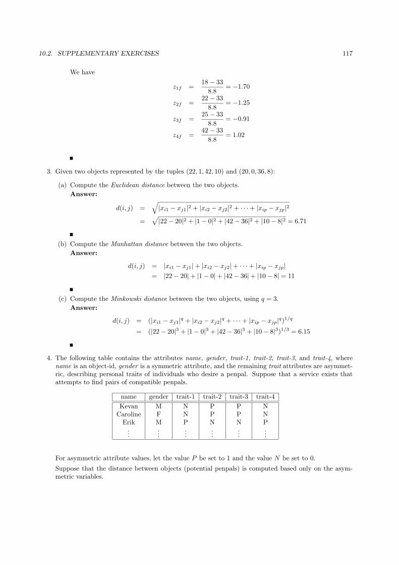
10.2. SUPPLEMENTARY EXERCISES 117
We have
z1f =18− 33
8.8= −1.70
z2f =22− 33
8.8= −1.25
z3f =25− 33
8.8= −0.91
z4f =42− 33
8.8= 1.02
3. Given two objects represented by the tuples (22, 1, 42, 10) and (20, 0, 36, 8):
(a) Compute the Euclidean distance between the two objects.
Answer:
d(i, j) =√|xi1 − xj1|2 + |xi2 − xj2|2 + · · ·+ |xip − xjp|2
=√|22− 20|2 + |1− 0|2 + |42− 36|2 + |10− 8|2 = 6.71
(b) Compute the Manhattan distance between the two objects.
Answer:
d(i, j) = |xi1 − xj1|+ |xi2 − xj2|+ · · ·+ |xip − xjp|= |22− 20|+ |1− 0|+ |42− 36|+ |10− 8| = 11
(c) Compute the Minkowski distance between the two objects, using q = 3.
Answer:
d(i, j) = (|xi1 − xj1|q + |xi2 − xj2|q + · · ·+ |xip − xjp|q)1/q
= (|22− 20|3 + |1− 0|3 + |42− 36|3 + |10− 8|3)1/3 = 6.15
4. The following table contains the attributes name, gender, trait-1, trait-2, trait-3, and trait-4, wherename is an object-id, gender is a symmetric attribute, and the remaining trait attributes are asymmet-ric, describing personal traits of individuals who desire a penpal. Suppose that a service exists thatattempts to find pairs of compatible penpals.
name gender trait-1 trait-2 trait-3 trait-4
Kevan M N P P NCaroline F N P P NErik M P N N P...
......
......
...
For asymmetric attribute values, let the value P be set to 1 and the value N be set to 0.
Suppose that the distance between objects (potential penpals) is computed based only on the asym-metric variables.
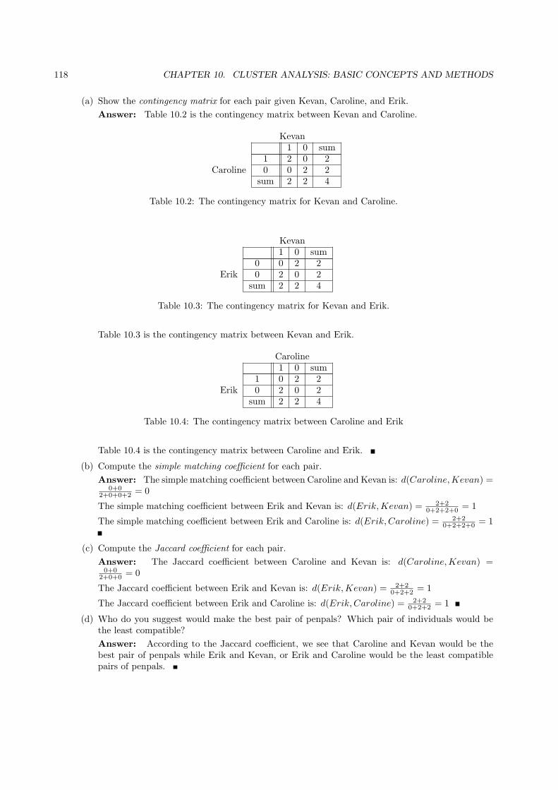
118 CHAPTER 10. CLUSTER ANALYSIS: BASIC CONCEPTS AND METHODS
(a) Show the contingency matrix for each pair given Kevan, Caroline, and Erik.
Answer: Table 10.2 is the contingency matrix between Kevan and Caroline.
Kevan1 0 sum
1 2 0 2Caroline 0 0 2 2
sum 2 2 4
Table 10.2: The contingency matrix for Kevan and Caroline.
Kevan1 0 sum
0 0 2 2Erik 0 2 0 2
sum 2 2 4
Table 10.3: The contingency matrix for Kevan and Erik.
Table 10.3 is the contingency matrix between Kevan and Erik.
Caroline1 0 sum
1 0 2 2Erik 0 2 0 2
sum 2 2 4
Table 10.4: The contingency matrix between Caroline and Erik
Table 10.4 is the contingency matrix between Caroline and Erik.
(b) Compute the simple matching coefficient for each pair.
Answer: The simple matching coefficient between Caroline and Kevan is: d(Caroline,Kevan) =0+0
2+0+0+2 = 0
The simple matching coefficient between Erik and Kevan is: d(Erik,Kevan) = 2+20+2+2+0 = 1
The simple matching coefficient between Erik and Caroline is: d(Erik, Caroline) = 2+20+2+2+0 = 1
(c) Compute the Jaccard coefficient for each pair.
Answer: The Jaccard coefficient between Caroline and Kevan is: d(Caroline,Kevan) =0+0
2+0+0 = 0
The Jaccard coefficient between Erik and Kevan is: d(Erik,Kevan) = 2+20+2+2 = 1
The Jaccard coefficient between Erik and Caroline is: d(Erik, Caroline) = 2+20+2+2 = 1
(d) Who do you suggest would make the best pair of penpals? Which pair of individuals would bethe least compatible?
Answer: According to the Jaccard coefficient, we see that Caroline and Kevan would be thebest pair of penpals while Erik and Kevan, or Erik and Caroline would be the least compatiblepairs of penpals.

10.2. SUPPLEMENTARY EXERCISES 119
(e) Suppose that we are to include the symmetric variable gender in our analysis. Based on theJaccard coefficient, who would be the most compatible pair, and why?
Answer: The Jaccard coefficient for each pair are calculated as follows:
d(Caroline,Kevan) = 11+1+1 = 1
3
d(Erik,Kevan) = 1+1+1+11+1+1+1+1 = 4
5
d(Erik, Caroline) = 1+1+1+11+1+1+1 = 1
Based on the above, Caroline and Kevan would still be the most compatible pair since the Jaccardcoefficient between them is the smallest.
5. Use a diagram to illustrate how, for a constant MinPts value, density-based clusters with respect to ahigher density (i.e., a lower value for ϵ, the neighborhood radius) are completely contained in density-connected sets obtained with respect to a lower density.
Answer: See the diagram of Figure 10.1. Note that C1 and C2 are density-based clusters withrespect to ϵ2 < ϵ1, and C is a density-based cluster with respect to ϵ1 which completely contains thesets C1 and C2. (MinPts = 3.)
C
C2C1
e1e2
Figure 10.1: A diagram illustrating concepts of density-based clusters.
6. Use an example to show why CLARA may not find good clustering even if the sample size is large andin an equal probability of selection design.
7. Jaccard coefficient has been used as a similarity measure for (asymmetric) binary and categorical data.However, we have shown that the link measure based on counting the number of common neighborsproposed in ROCK may lead to better clustering quality. Can you identify at what situations that theformer (Jaccard coefficient) may lead to better quality cluster than the latter, and vice versa?
8. Many clustering algorithms handle either only numerical data, such as BIRCH, or only categorical data,such as ROCK, but not both. Analyze why this is the case. Note, however, that the EM clusteringalgorithm can easily be extended to handle data with both numerical and categorical attributes. Brieflyexplain why it can do so and how.
Answer: EM clustering essentially uses an underlying mixture model to do clustering. It is dueto the probabilistic nature of such models that we can easily extend EM clustering to handle datawith both numerical attributes and categorical attributes. Under the assumption that each attributeis independent of each other, we

120 CHAPTER 10. CLUSTER ANALYSIS: BASIC CONCEPTS AND METHODS
we could model numerical attributes by using density functions such as Poission, Gaussian, etc, andmodel categorical attributes by associating discrete distribution over these attributes such as Multino-mial, Binomial, etc. The total component density can be decomposed as a product of density functionsover each attribute. By having such component density functions, we will be able to easily use EMclustering to cluster data with both numerical attributes and categorical attributes.
Reference: Paul S. Bradley Usama M. Fayyad Cory A, Scaling EM (Expectation-Maximization) Clus-tering to Large Databases, Technical Report, Microsoft Research Microsoft Corporation, October 1999.
9. Give an example of how specific clustering methods may be integrated, for example, where one clusteringalgorithm is used as a preprocessing step for another.
Answer: One example could be Birch, a method that integrates hierarchical clustering with otherclustering techniques for multiple phase clustering. It begins by partitioning objects hierarchicallyusing tree structures, and then applies other clustering algorithms to refine the clusters. BIRCHincrementally constructs a CF(Clustering Feature) tree, which is a height-balanced tree that stores theclustering features for a hierarchical clustering. This method consists of two phases. Phase 1 scans thedatabase to build an initial in-memory CF tree, which can be viewed as a multilevel compression of thedata that tries to preserve the inherent clustering structure of the data. Phase 2 applies an arbitraryclustering algorithm to cluster the leaf nodes of the CF-tree. It therefore uses the hierarchical clusteringtechnique as a preprocessing step.
10. Clustering has been popularly recognized as an important data mining task with broad applications.Give one application example for each of the following cases:
(a) An application that takes clustering as a major data mining function
Answer: An example that takes clustering as a major data mining function could be a systemthat identifies groups of houses in a city according to house type, value, and geographical location.More specifically, a clustering algorithm like CLARANS can be used to discover that, say, themost expensive housing units in Vancouver can be grouped into just a few clusters.
(b) An application that takes clustering as a preprocessing tool for data preparation for other datamining tasks
Answer: An example application that takes clustering as a preprocessing tool for other datamining is spatial data mining. Spatial data mining is the discovery of interesting relationships andcharacteristics that may exist implicitly in spatial databases. We can apply cluster analysis only tospatial attributes, where natural notions of similarity exist. Various clustering algorithms, such asPAM, CLARA, or CLARANS may be used. The clusters obtained from the clustering algorithmmay trigger the generation on non-spatial components in the next step if such a generation cangroup objects into interesting groups.
11. Data cubes and multidimensional databases contain categorical, ordinal, and numerical data in hier-archical or aggregate forms. Based on what you have learned about the clustering methods, design aclustering method that finds clusters in large data cubes effectively and efficiently.
Answer: We can use the idea of a grid-based clustering approach, such as the CLIQUE, to find thecluster in a large data cube since a data cube can be interpreted as a multiresolution grid data structure.We first need to preprocess and discretize existing data (such as ordinal, numerical data) in order toobtain a single dimensional discretization. We then can perform the multidimensional clustering intwo steps. The first step involves partitioning of the n-dimensional data space into non-overlappingrectangular units, identifying the dense units among these. This is done in 1-D for each dimension.We then can generate candidate dense units in k-dimensional space from the dense units found in(k− 1)-dimensional space. In the second step, a minimal description for each cluster is generated. Foreach cluster, this determines the maximal region that covers the cluster of connected dense units. It
10.2. SUPPLEMENTARY EXERCISES 121
then determines a minimal cover for each cluster. Using such a method, we can effectively find clustersfrom the data that are represented as a data cube.
12. Why is outlier mining important? Briefly describe the different approaches behind statistical-basedoutlier detection, distance-based outlier detection, and deviation-based outlier detection.
Answer: Data objects that are grossly different from, or inconsistent with, the remaining set of dataare called “outliers”. Outlier mining is useful for detecting fraudulent activity, (such as credit cardor telecom fraud), as well as customer segmentation and medical analysis. Computer-based outlieranalysis may be statistical-based, distance-based, or deviation-based.
The statistical-based approach assumes a distribution or probability model for the given data set andthen identifies outliers with respect to the model using a discordancy test. The discordancy test isbased on data distribution, distribution parameters (e.g., mean, variance), and the number of expectedoutliers. The drawbacks of this method are that most tests are for single attributes, and in many cases,the data distribution may not be known.
The distance-based approach was introduced to counter the limitations of the statistical-based ap-proach. A DB(p,D)-outlier is an object O in a data set T such that at least a fraction p of the objectsin T lies at a distance greater than D from O. In comparison with the statistical-based approach,the distance-based approach generalizes the idea behind discordancy testing for various standard dis-tributions. Moreover, the distance-based outlier detection avoids the excessive computation that canbe associated with fitting the observed distribution into some standard distribution and in selectingdiscordancy tests.
The deviation-based outlier detection does not use statistical tests or distance-based measures to iden-tify exceptional object. Instead, it identifies outliers by examining the main characteristics of objectsin a group. Objects that “deviate” from this description are considered outliers. Two techniques forthis method approach include a sequential exception technique and an OLAP data cube technique.

122 CHAPTER 10. CLUSTER ANALYSIS: BASIC CONCEPTS AND METHODS

Chapter 11
Advanced Cluster Analysis
11.1 Exercises
1. Traditional clustering methods are rigid in that they require each object to belong exclusively to onlyone cluster. Explain why this is a special case of fuzzy clustering. You may use k-means as an example.
Answer:
k-means can be regarded as a special case of fuzzy clustering. The corresponding partition matrix isthat, if object oi belongs to cluster Cj , then wij = 1 and the other entries on the i-th row are 0. Itis easy to verify that the partition matrix M defined as such satisfies all the three requirements for apartition matrix in fuzzy clustering.
2. AllElectronics carries 1, 000 products, P1, . . . , P1000. Consider customers Ada, Bob, and Cathy suchthat Ada and Bob purchase three products in common, P1, P2, and P3. For the other 997 products, Adaand Bob independently purchase seven of them randomly. Cathy purchases ten products, randomlyselected from the 1, 000 products. In Euclidean distance, what is the probability that dist(Ada,Bob) >dist(Ada,Cathy)? What if Jaccard similarity (Chapter 2) is used? What can you learn from thisexample?
Answer:
The probability that Ada and Bob choose i (3 ≤ i ≤ 10) common products is
Pr1(i) =
(9977
)(7
i− 3
)(990
10− i
)(9977
)2 =
(7
i− 3
)(990
10− i
)(9977
)Varying i from 3 to 10, we have the following table.
i 3 4 5 6
dist(Ada, Bob)√14 = 3.7
√12 = 3.5
√10 = 3.2
√8 = 2.8
J(Ada, Bob) 317 = 0.18 4
16 = 0.25 515 = 0.33 6
14 = 0.43Pr1(i) 0.95 6.8× 10⁻³ 4.1× 10⁻⁵ 2.1× 10⁻⁷
i 7 8 9 10
dist(Ada, Bob)√6 = 2.4
√4 = 2
√2 = 1.4
√0 = 0
J(Ada, Bob) 714 = 0.5 8
12 = 0.67 911 = 0.82 10
10 = 1Pr1(i) 8.5× 10⁻¹⁰ 2.6× 10⁻¹² 5.2× 10⁻¹⁵ 5.3× 10⁻¹⁸
123
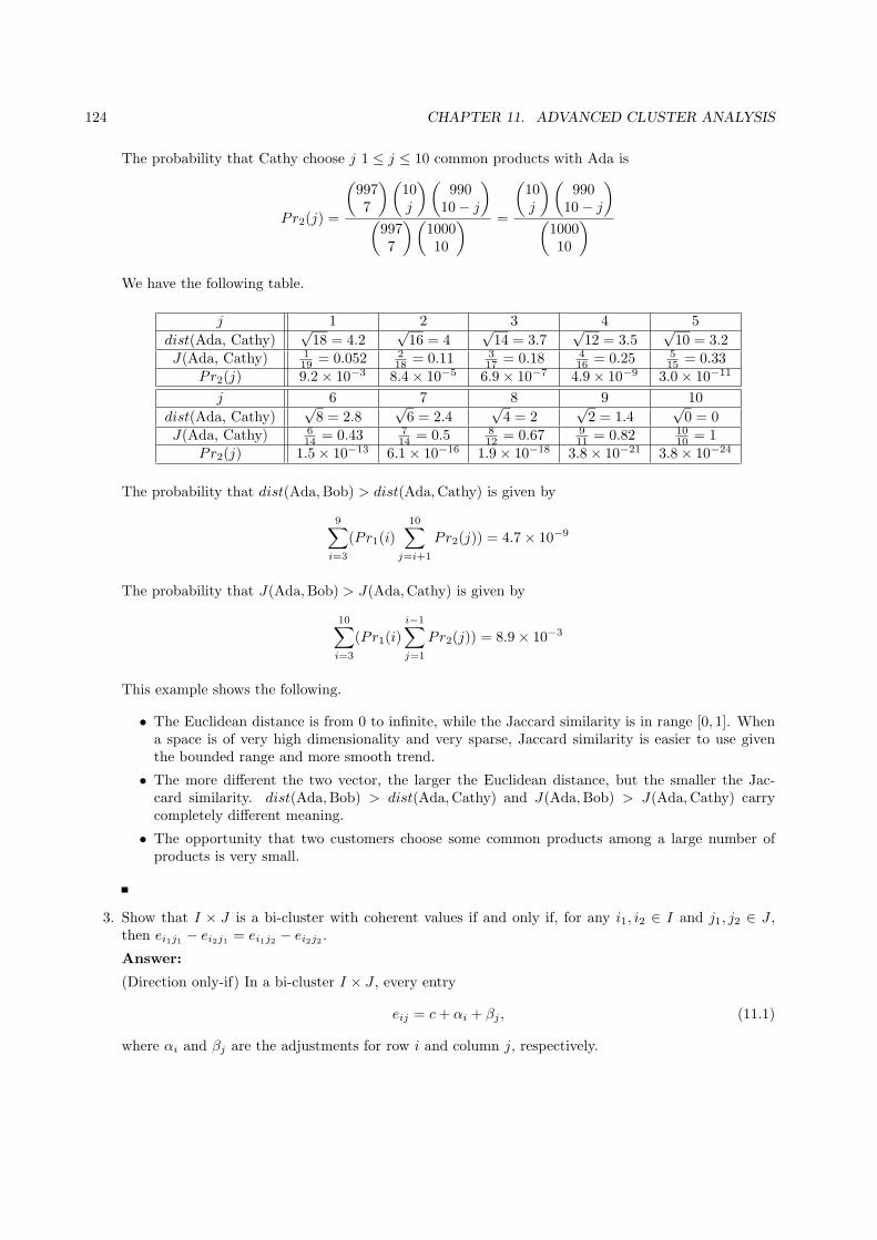
124 CHAPTER 11. ADVANCED CLUSTER ANALYSIS
The probability that Cathy choose j 1 ≤ j ≤ 10 common products with Ada is
Pr2(j) =
(9977
)(10j
)(990
10− j
)(9977
)(100010
) =
(10j
)(990
10− j
)(100010
)We have the following table.
j 1 2 3 4 5
dist(Ada, Cathy)√18 = 4.2
√16 = 4
√14 = 3.7
√12 = 3.5
√10 = 3.2
J(Ada, Cathy) 119 = 0.052 2
18 = 0.11 317 = 0.18 4
16 = 0.25 515 = 0.33
Pr2(j) 9.2× 10⁻³ 8.4× 10⁻⁵ 6.9× 10⁻⁷ 4.9× 10⁻⁹ 3.0× 10⁻¹¹
j 6 7 8 9 10
dist(Ada, Cathy)√8 = 2.8
√6 = 2.4
√4 = 2
√2 = 1.4
√0 = 0
J(Ada, Cathy) 614 = 0.43 7
14 = 0.5 812 = 0.67 9
11 = 0.82 1010 = 1
Pr2(j) 1.5× 10⁻¹³ 6.1× 10⁻¹⁶ 1.9× 10⁻¹⁸ 3.8× 10⁻²¹ 3.8× 10⁻²⁴
The probability that dist(Ada,Bob) > dist(Ada,Cathy) is given by
9∑i=3
(Pr1(i)10∑
j=i+1
Pr2(j)) = 4.7× 10⁻⁹
The probability that J(Ada,Bob) > J(Ada,Cathy) is given by
10∑i=3
(Pr1(i)
i−1∑j=1
Pr2(j)) = 8.9× 10⁻³
This example shows the following.
• The Euclidean distance is from 0 to infinite, while the Jaccard similarity is in range [0, 1]. Whena space is of very high dimensionality and very sparse, Jaccard similarity is easier to use giventhe bounded range and more smooth trend.
• The more different the two vector, the larger the Euclidean distance, but the smaller the Jac-card similarity. dist(Ada,Bob) > dist(Ada,Cathy) and J(Ada,Bob) > J(Ada,Cathy) carrycompletely different meaning.
• The opportunity that two customers choose some common products among a large number ofproducts is very small.
3. Show that I × J is a bi-cluster with coherent values if and only if, for any i1, i2 ∈ I and j1, j2 ∈ J ,then ei1j1 − ei2j1 = ei1j2 − ei2j2 .
Answer:
(Direction only-if) In a bi-cluster I × J , every entry
eij = c+ αi + βj , (11.1)
where αi and βj are the adjustments for row i and column j, respectively.

11.1. EXERCISES 125
Applying Equation 11.1, we have ei1j1 − ei2j1 = c + αi1 + βj1 − c − αi2 − βj1 = αi1 − αi2 . Similarly,ei1j2 − ei2j2 = αi1 − αi2 . Thus, ei1j1 − ei2j1 = ei1j2 − ei2j2 .
(Direction if) Let c = −e11, αi = ei1 and βj = e1j .
Since for any i1, i2 ∈ I and j1, j2 ∈ J , ei1j1 − ei2j1 = ei1j2 − ei2j2 , we have eij − e1j = ei1− e11. Thatis, eij = −e11 + ei1 + e1j = c+ αi + βj . I × J is a bi-cluster with coherent values.
4. Compare the MaPle algorithm (Section 11.2.3) with the frequent closed-itemset mining algorithm,CLOSET (Pei, Han, and Mao [PHM00]). What are the major similarities and differences?
Answer:
In frequent closed-itemset mining, we can start with frequent items. However, in maximal δ-pClustermining, a δ-pCluster has at least two rows and two columns. We need a step to find all δ-pClustersof at least 2 rows or 2 columns. Moreover, while the two methods carry similar ideas in pruning, thetechnical details are different.
5. SimRank is a similarity measure for clustering graph and network data.
(a) Prove limi→∞
si(u, v) = s(u, v) for SimRank computation.
(b) Show s(u, v) = p(u, v) for SimRank.
Answer:
Please refer to [JW02].
6. In a large sparse graph where on average each node has a low degree, is the similarity matrix usingSimRank still sparse? If so, in what sense? If not, why? Deliberate on your answer.
Answer:
Theoretically, even when the average degree is low, as long as the graph is connected, the similaritymatrix is not sparse at all, since every entry in the matrix has a non-zero value.
When an approximation is used wherein entries of very small values are set to 0, the similarity matrixusing SimRank may be sparse when the average degree is low. In fact, the sparsity of the matrix isrelated to the average size of the k-neighborhoods of nodes, since if two nodes are k steps or moreaway, the SimRank between them can be set to 0, where k is a small number, such as 2 or 3.
For the detailed discussion, please refer to [JW02].
7. Compare the SCAN algorithm (Section 11.3.3) with DBSCAN (Chapter 6). What are their similaritiesand differences?
Answer:
Similarities Both methods are density-based, and follow similar frameworks. Both use the mecha-nisms of ϵ-neighborhoods and core objects/vertices to grow clusters.
Differences The similarity between points in DBSCAN and that between vertices in SCAN are dif-ferent, due to the different types of data. SCAN identifies hubs and outliers. DBSCAN does notfind any hub points.

126 CHAPTER 11. ADVANCED CLUSTER ANALYSIS
8. Consider partitioning clustering and the following constraint on clusters: the number of objects in eachcluster must be between n
k (1 − δ) and nk (1 + δ), where n is the total number of objects in the data
set, k is the number of clusters desired, and δ in [0, 1) is a parameter. Can you extend the k-meansmethod to handle this constraint? Discuss situations where the constraint is hard and soft.
Answer:
There may exist other feasible answers different from the following.
If the constraint is hard, that is, cannot be violated, we can extend the k-means algorithm with thefollowing changes in the assignment step.
Suppose c1, . . . , ck are the current k centers (means).
(a) For each point p, calculate p.MinDist = minki=1{dist(p, ci)}, and p.CId = argminki=1{dist(p, ci)},that is, the distance to the closest center and the id of the closest center.
(b) Process all points in MinDist increasing order. For a point p, if p.CId has been assigned lessthan n
k (1 − δ) points, assign p to p.CId. Otherwise, update p.MinDist to the distance betweenp and the next closest center that has been assigned less than n
k (1− δ) points, and let p.CId bethat center.
After this step, every center is assigned nk (1− δ) points.
(c) For the remaining, unassigned points, calculate p.MinDist = minki=1{dist(p, ci)}, and p.CId =argminki=1{dist(p, ci)}, that is, the distance to the closest center and the id of the closest center.
Process all points in MinDist increasing order. For a point p, if p.CId has been assigned lessthan n
k (1 + δ) points, assign p to p.CId. Otherwise, update p.MinDist to the distance betweenp and the next closest center that has been assigned less than n
k (1 + δ) points, and let p.CId bethat center.
After this step, every center is assigned at most nk (1 + δ) points.
When the constraint is soft, we can use a penalty function that penalizes a clustering more if a centeris assigned much less than n
k (1− δ) points or much more than nk (1+ δ) points. Such a penalty function
can integrate the penalty with the within-cluster variation. For example, consider a clustering C whosewithin-cluster variation is E. Let c1, . . . , ck are the centers, and |Ci| (1 ≤ i ≤ k) are the number of
points assigned to ci. The penalty function can be E′ = E +∑k
i=1 di, where
di =
(nk (1− δ)− |Ci|) · avgdist if |Ci| < n
k (1− δ)
(|Ci| − nk (1 + δ)) · avgdist if |C1| > n
k (1 + δ)
0 otherwise
and avgdist is the average distance between two points in the data set. The revised k-means algorithmshould try to minimize E′.

Chapter 12
Outlier Detection
12.1 Exercises
1. Give an application example where global outliers, contextual outliers and collective outliers are allinteresting. What are the attributes, and what are the contextual and behavioral attributes? How isthe relationship among objects modeled in collective outlier detection?
Answer:
A credit card company often maintains a profile for each customer. Suppose a profile has the fol-lowing attributes: name, age, job, address, annual-income, annual-expense, average-balance,credit-limit. Global outliers, contextual outliers, and collective outliers are all interesting.
• A global outlier is interesting, since it may be a customer who are very different from the majorityof customers of the company. The significant difference may call for special service or monitoringby the company.
• Consider annual-income and annual-expense as the contextual attributes, and average-balanceas the behavior attribute. A contextual outlier is interesting, since its usage of the credit cardis dramatically different from the other customers in the same group. Such an outlier customer,for example, may either spend much less or much more than the others in the same contextualgroup. If the outlier customer spends much less, than the company can try to promote servicesto the customer. On the other hand, if the customer spends much more, than the company caneither introduce special service to encourage even more spending, or apply special monitoring toprevent from frauds or bad credit behaviors, depending on the nature of the spending.
Please note that a contextual outlier’s average balance may still within the normal range for allcustomers, and thus is not a global outlier.
• Suppose the credit card company finds a group of customers from a geographically proximate area(through the attribute address) have very low annual-income but very high annual-expense,which is substantially different from the other customers. This forms a group of collective outliers.This is interesting to the company, since this group of customers may need to be monitored closelyand their credit limits may need to be controlled firmly.
2. Give an application example of where the border between “normal objects” and outliers is often unclear,so that the degree to which an object is an outlier has to be well estimated.
Answer:
127

128 CHAPTER 12. OUTLIER DETECTION
A credit card company has to monitor credit card transactions. However, the border between “normaltransactions” and outliers, such as frauds, is often unclear, because the distinction between the twooften depends on many other factors not included in the transactions themselves. Therefore, a goodfraud detection system in a credit card company, which is essentially an outlier detection system, hasto estimate the degree to which a transaction is an outlier.
3. Adapt a simple semi-supervised method for outlier detection. Discuss the scenario where you have i)only some labeled examples of “normal objects”, and ii) only some labeled examples of outliers.
Answer:
When only some labeled examples are available, we can take use those examples to learn a modelfor the normal objects. For example, we may use a density-based approach to find dense areas thatcontain at least one normal objects. The objects falling into those areas can be regarded as normal.The objects that are far away from any normal objects are candidates of outliers.
When only some labeled examples of outliers are available, we may use those examples to extract thefeatures that can distinguish outliers. That is, we may extract a minimal set of features such that,according to those features, the labeled outlier examples are far away from most of the unlabeledobjects, and most of the unlabeled objects form clusters. Then, those unlabeled objects falling intoclusters can be regarded as normal, and the objects far away from those clusters are candidates ofoutliers.
4. Using an equi-depth histogram, design a way to assign an object an outlier score.
Answer:
We observe that in an equi-depth histogram, a narrower bucket contains points that are more similarto each other than a wider bucket. Based on this observation, a possible way to assign an object anoutlier score is as follows. For each bucket Bi, denote by li the width of the bucket. Then, for anobject falling into the bucket Bi, we assign the outlier score li. The larger the outlier score, the morelikely the object is an outlier.
5. Consider the nested loop approach to mining distance-based outliers (Figure ??). Suppose the objectsin a data set are arranged randomly, that is, each object has the same probability to appear in aposition. Show that when the number of outlier objects is small with respect to the total number ofobjects in the whole data set, the expected number of distance calculations is linear to the number ofobjects.
Answer:
Please refer to [BS03].
6. In the density-based outlier detection method of Section ??, the definition of local reachability densityhas a potential problem: lrdk(o) = ∞ may occur. Explain why this may occur and propose a fix tothe issue.
Answer:
For an object o, if there are another k objects located at the same position, then lrdk(o) =∞. To fixthis problem, we can use a parameter ϵ > 0 and set dist(o, o′) = max{d(o, o′), ϵ}, where d(o, o′) givesthe distance between o and o′.

12.1. EXERCISES 129
o
Figure 12.1: Outlier o cannot be detected by the angle-based method.
7. Because clusters may form a hierarchy, outliers may belong to different levels of granularity. Proposea clustering-based outlier detection method that can find outliers at different levels.
Answer:
A possible method is to use probabilistic hierarchical clustering to learn a hierarchy of clusters. At eachcluster in the hierarchy, we can calculate the probability of each sub-cluster and use this probabilityas the outlier score – the lower the probability, the more likely it is an outlier.
As another example, we may use density-based clustering method. At the global level, we can use alarge radius or a small neighborhood density threshold to form clusters. At a lower level, we can usea smaller radius or a larger neighborhood density threshold to find subclusters within a higher levelcluster. Once a hierarchy of clusters is formed, we can then apply the density-based outlier detectionmethod to find outliers within each cluster. The parameters should be set properly according to theparameter values used to find those clusters.
8. In outlier detection by semi-supervised learning, what is the advantage of using objects without labelsin the training data set?
Answer:
Since semi-supervised outlier detection methods assume that only some of the normal objects andoutliers are labeled, or in some cases even no outliers are labeled, they are more widely applicable thansupervised outlier detection methods. Semi-supervised outlier detection methods can make good useof the available unlabeled data, and build a more reliable model when the amount of labeled data issmall.
9. To understand why angle-based outlier detection is a heuristic method, give an example where it doesnot work well. Can you come up with a method to overcome this issue?
Answer:
Consider the situation as shown in Figure 12.1. The angle-based outlier factor of o is big, however, itis an outlier.

130 CHAPTER 12. OUTLIER DETECTION

Chapter 13
Trends and Research Frontiers inData Mining
13.1 Exercises
1. Sequence data are ubiquitous and have diverse applications. This chapter presented a general overviewof sequential pattern mining, sequence classification, sequence similarity search, trend analysis, biolog-ical sequence alignment and modeling. However, we have not covered sequence clustering. Present anoverview of methods for sequence clustering.
Answer:
Sequence clustering algorithms have been used widely in bioinformatics, attempting to group sequencesthat are somehow related. The sequences can be either of genomic, “transcriptomic” (ESTs) or proteinorigin. For proteins, homologous sequences are typically grouped into families. For EST data, clusteringis important to group sequences originating from the same gene before the ESTs are assembled toreconstruct the original mRNA.
Some clustering algorithms use single-linkage clustering, constructing a transitive closure of sequenceswith a similarity over a particular threshold. UCLUST and CD-HIT use a greedy algorithm thatidentifies a representative sequence for each cluster and assigns a new sequence to that cluster if it issufficiently similar to the representative; if a sequence is not matched then it becomes the representativesequence for a new cluster. The similarity score is often based on sequence alignment. Sequenceclustering is often used to make a non-redundant set of representative sequences. Sequence clusters areoften synonymous with (but not identical to) protein families. Determining a representative tertiarystructure for each sequence cluster is the aim of many structural genomics initiatives.
Here are some sequence clustering packages using in bioinformatics: (1) UCLUST: An exceptionallyfast sequence clustering program for nucleotide and protein sequences, (2) TribeMCL: a method forclustering proteins into related groups, (3) BAG: a graph theoretic sequence clustering algorithm,(4) CD-HIT: an ultra-fast method for clustering protein and nucleotide sequences, with many newapplications in next generation sequencing (NGS) data, (5) JESAM: Open source parallel scalableDNA alignment engine with optional clustering software component, (6) UICluster: Parallel Clusteringof EST (Gene) Sequences, (7) BLASTClust: single-linkage clustering with BLAST, (8) Clusterer:extendable java application for sequence grouping and cluster analyses, (9) PATDB: a program forrapidly identifying perfect substrings, (10) nrdb: a program for merging trivially redundant (identical)sequences, (11) CluSTr: A single-linkage protein sequence clustering database from Smith-Watermansequence similarities; covers over 7 mln sequences including UniProt and IPI, (12) ICAtools - original(ancient) DNA clustering package with many algorithms useful for artifact discovery or EST clustering,
131
132 CHAPTER 13. TRENDS AND RESEARCH FRONTIERS IN DATA MINING
(13) Virus Orthologous Clusters: A viral protein sequence clustering database; contains all predictedgenes from eleven virus families organized into ortholog groups by BLASTP similarity.
A method for sequence clustering for general categorical data sequences is as follows (for details, see J.Yang and W. Wang, “CLUSEQ: Efficient and effective sequence clustering”, ICDE’03). One difficultythat prevents clustering from being performed extensively on sequence data (in categorical domain)is the lack of an effective yet efficient similarity measure. CLUSEQ explores significant statisticalproperties possessed by the sequences. The conditional probability distribution (CPD) of the nextsymbol given a preceding segment is derived and used to characterize sequence behavior and to supportthe similarity measure. A variation of the suffix tree, namely probabilistic suffix tree, is employed toorganize (the significant portion of) the CPD in a concise way. The method efficiently discovers clusterswith high quality and is able to automatically adjust the number of clusters to its optimal range via aunique combination of successive new cluster generation and cluster consolidation.
A more comprehensive survey could be a good student course project.
2. This chapter presented an overview of sequence pattern mining and graph pattern mining methods.Mining tree patterns and partial order patterns are also studied in research. Summarize the methods formining structured patterns, including sequences, trees, graphs, and partial order relationships. Examinewhat kinds of structural pattern mining have not been covered in research. Propose applications thatcan be created for such new mining problems.
Answer:
For a summary of methods for mining structured patterns, including sequences, trees, graphs, andpartial order relationships, please see: Jiawei Han, Hong Cheng, Dong Xin, and Xifeng Yan, “FrequentPattern Mining: Current Status and Future Directions”, Data Mining and Knowledge Discovery, 15(1):55-86, 2007.
There are still aspects not covered in research on structural pattern mining. For example, how to minecolossal structured patterns in large data sets (e.g., finding rather large frequent subnetwork patternsin one or a set of large networks), how to semantically annotate structured patterns, similar to thosethat has been done for semantic annotation of frequent patterns (please see Q. Mei, D. Xin, H. Cheng,J. Han, and C. Zhai, “Semantic annotation of frequent patterns”, ACM Transactions on KnowledgeDiscovery from Data, 1(3), 11:1-28, 2007).
3. Many studies analyze homogeneous information networks, e.g., social networks consisting of friendslinked with friends. However, many other applications involve heterogeneous information networks,i.e., networks linking multiple types of object, such as research papers, conference, authors, and topics.What are the major differences between methodologies for mining heterogeneous information networksand methods for their homogeneous counterparts?
Answer:
In homogeneous information networks, nodes in a network are of the same type and the measuresand methods for studying the network behavior are similar to typical graph algorithms. However,in heterogeneous information networks, since the networks are formed by linking multiple types ofobject, such as research papers, conference, authors, and topics, the measure of similarity for nodesin the network, and methods for mining knowledge in a network are rather different from that ofmining homogeneous information networks. Multiple studies have been done on this topic. For a fewinteresting studies, please read the following papers:
(a) Yizhou Sun, Jiawei Han, Xifeng Yan, Philip S. Yu, and Tianyi Wu, “PathSim: Meta Path-BasedTop-K Similarity Search in Heterogeneous Information Networks”, Proc. of 2011 Int. Conf. on VeryLarge Data Bases (VLDB’11), Seattle, WA, Aug. 2011.

13.1. EXERCISES 133
(b) Ming Ji, Jiawei Han, and Marina Danilevsky, “Ranking-Based Classification of HeterogeneousInformation Networks”, Proc. of 2011 ACM SIGKDD Int. Conf. on Knowledge Discovery and DataMining (KDD’11), San Diego, Aug. 2011.
(c) Yizhou Sun, Yintao Yu, and Jiawei Han, “Ranking-Based Clustering of Heterogeneous InformationNetworks with Star Network Schema”, Proc. 2009 ACM SIGKDD Int. Conf. on Knowledge Discoveryand Data Mining (KDD’09), Paris, France, June 2009.
(d) Yizhou Sun, Rick Barber, Manish Gupta, Charu Aggarwal and Jiawei Han, “Co-Author Relation-ship Prediction in Heterogeneous Bibliographic Networks”, Proc. of 2011 Int. Conf. on Advances inSocial Network Analysis and Mining (ASONAM’11), Kaohsiung, Taiwan, July 2011.
(e) Yizhou Sun, Jiawei Han, Charu C. Aggarwal, and Nitesh Chawla, “When Will It Happen? —Relationship Prediction in Heterogeneous Information Networks”, Proc. 2012 ACM Int. Conf. onWeb Search and Data Mining (WSDM’12), Seattle, WA, Feb. 2012.
4. Research and describe an application of data mining that was not presented in this chapter. Discusshow different forms of data mining can be used in the application.
Answer:
There are many application areas that are not covered in this chapter. Thus you can answer anythingyou believe it is fresh and interesting.
For example, one can consider an Earth observation system that may watch the changes of Earthsurfaces and climates. Obviously, this belongs to the domain of very long-term spatiotemporal datamining, and many new techniques need to be developed to effectively mine such data sets.
5. Study an existing commercial data mining system. Outline the major features of such a system from amultidimensional point of view, including data types handled, architecture of the system, data sources,data mining functions, data mining methodologies, coupling with database or data warehouse systems,scalability, visualization tools, and graphical user interfaces. Can you propose one improvement tosuch a system and outline how to realize it?
Answer:
There are many systems one can study, such as Microsoft SQL Server, SAS EnterpriseMiner, IBM Intel-ligentMiner, SGI MineSet, and SPSS Clementine. Here is one short summary on Microsoft SQLServer,based on its 2005 version (newer versions are available and need to be summarized if one has time.)
SQLServer is an multi-function data mining system, developed for integrative mining of multiple kindsof knowledge in large relational databases and data warehouses. The major distinguishing feature ofthe SQLServer system is its tight integration of the data mining subsystem with the relational databaseand data warehouse subsystems in the same system, and its natural integration with multiple Microsofttools, such as Excel, Web publishing, etc. It provides multiple data mining functions, including as-sociation, classification, prediction, and clustering. This integration leads to a promising data miningmethodology that integrates multi-dimensional online processing and data mining, where the systemprovides a multidimensional view of its data and creates an interactive data mining environment. Thesystem facilitates query-based interactive mining of multidimensional databases by implementing aset of advanced data mining techniques. SQLServer integrates smoothly with relational database anddata warehouse systems to provide a user-friendly, interactive data mining environment with highperformance.

134 CHAPTER 13. TRENDS AND RESEARCH FRONTIERS IN DATA MINING
6. (Research project) Relational database query languages, like SQL, have played an essential rolein the development of relational database systems. Similarly, a data mining query language mayprovide great flexibility for users to interact with a data mining system and pose various kinds of datamining queries and constraints. It is expected that different data mining query languages may bedesigned for mining different types of data (such as relational, text, spatiotemporal, and multimediadata) and for different kinds of applications (such as financial data analysis, biological data analysis,and social network analysis). Select an application. Based on your application requirements and thetypes of data to be handled, design such a data mining language and study its implementation andoptimization issues.
Answer:
A good research topic with no definite answer, especially considering that the length of the answercould be as long as a thesis.
7. Why is the establishment of theoretical foundations important for data mining? Name and describethe main theoretical foundations that have been proposed for data mining. Comment on how theyeach satisfy (or fail to satisfy) the requirements of an ideal theoretical framework for data mining.
Answer:
In general, the establishment of theoretical foundation is important for data mining because it can helpprovide a coherent framework for the development, evaluation, and practice of data mining technology.The following are theories for the basis for data mining.
• Data reduction: The basis of data mining is to reduce the data representation. Data reductiontrades accuracy for speed in response to the need to obtain quick approximate answers to querieson very large databases.
• Data compression: According to this theory, the basis of data mining is to compress the givendata by encoding in terms of bits, association rules, decision trees, clusters, and so on. Encodingmay be based on the minimum description length principle.
• Pattern discovery: In this theory, the basis of data mining is to discover patterns occurring inthe database, such as association, classification models, sequential patterns, etc.
• Probability theory: This is based on statistical theory. The basis of data mining is to discoverjoint probability distributions of random variables.
• Microeconomic view: This theory considers data mining as the task of finding patterns thatare interesting only to the extent that they can be used in the decision-making process of someenterprise. Enterprises are considered as facing optimization problems where the object is tomaximize the utility or value of a decision. In this theory, data mining becomes a nonlinearoptimization problem.
• Inductive databases: According to this theory, a database schema consists of data and patternsthat are stored in the database. Data mining is the problem of performing induction on databases,where the task is to query the data and the theory of the database.
8. (Research project) Building a theory for data mining requires setting up a theoretical framework sothat the major data mining functions can be explained under this framework. Take one theory as anexample (e.g., data compression theory) and examine how the major data mining functions fit into thisframework. If some functions do not fit well into the current theoretical framework, can you proposea way to extend the framework to explain these functions?
Answer:

13.1. EXERCISES 135
This is a large research project. We do not have good answers. A good answer to such a questionshould be a research thesis.
9. There is a strong linkage between statistical data analysis and data mining. Some people think ofdata mining as automated and scalable methods for statistical data analysis. Do you agree or disagreewith this perception? Present one statistical analysis method that can be automated and/or scaled upnicely by integration with current data mining methodology.
Answer:
The perception of data mining as automated and scalable methods for statistical data analysis is aninteresting one and is true in many cases. For example, association mining is essentially the computationof conditional probability but it is done in an efficient and scalable way to handle very large data sets.Also, many clustering and classification algorithms can find some similar root in statistical analysisbut were re-examined in a scalable algorithmic way. However, there are methods developed in datamining that one may not find statistical counterpart. For example, many frequent pattern analysisproblems, such as sequential patterns, frequent substructures, etc. may not find their counterparts instatistical analysis. Also, there are also many sophisticated statistical analysis methods that have notbeen studied in data mining research.
10. What are the differences between visual data mining and data visualization? Data visualization maysuffer from the data abundance problem. For example, it is not easy to visually discover interestingproperties of network connections if a social network is huge, with complex and dense connections. Pro-pose a visualization method that may help people see through the network topology to the interestingfeatures of a social network.
Answer:
Data visualization is to present data in a visual way so that the data contents can be easily compre-hensible by human users. Pattern or knowledge visualization is to present patterns and knowledge ina visual way so that one can easily understand the regularities, patterns, outliers, and other formsof knowledge stored in or discovered from large data sets. Visual data mining is the process of datamining that presents data and patterns in a visually appealing and interactive way so that a user caneasily participate in the data mining process.
It is true that data visualization may suffer from the data abundance problem. Actually patterns cansuffer from the pattern abundance problems as well. In this case, one should be given primitives thatone can easily extract a portion of data or portions using constraints. This will be more focused andthe domain to be viewed is smaller. Another way is to provide multi-resolution capability so that atcertain level, only the data and patterns that are visible in the current resolution scala will be shown.The third way is to select only frequent or higher weighted nodes and labels in demonstration so thatcomplex connections can be simplified.
11. Propose a few implementation methods for audio data mining. Can we integrate audio and visualdata mining to bring fun and power to data mining? Is it possible to develop some video data miningmethods? State some scenarios and your solutions to make such integrated audiovisual mining effective.
Answer:
One approach for audio data mining is to transform data to sound or music. When we receive thepatterns, trends, structures and irregularity relationships from data mining, we need to transformthese data features into different pitches, rhythms, tunes, and melody in order to identify anythinginteresting or unusual. One technique is to establish mapping relations between color and music using

136 CHAPTER 13. TRENDS AND RESEARCH FRONTIERS IN DATA MINING
a universal music and color understanding and mapping method. It has been shown in recent researchthat some pieces of music can be mapped to universal color.
It is also possible to develop video data mining or other methods that integrates sound and image.The major task involved is the integration of audio and visual data mining in order to bring power todata mining. This requires combining visualization tools with the transformation of data patterns tosound, images, and videos, which also involves further development of methods for storing, accessingand demonstrating data efficiently in a multidimensional way. This is still a large and unexploredresearch domain.
12. General-purpose computers and domain-independent relational database systems have become a largemarket in the last several decades. However, many people feel that generic data mining systems willnot prevail in the data mining market. What do you think? For data mining, should we focus ourefforts on developing domain-independent data mining tools or on developing domain-specific datamining solutions? Present your reasoning.
Answer:
For data mining, there are general principles and algorithms that many data mining applications canuse. There are also specific algorithms that are aimed at solving particular practical problems, suchas searching biological sequence patterns. Even for general principles, more dedicated developmentsare often necessary due to different data characteristics to be mined on and different pattern to searchfor. Thus there should be two tracks in both research and development. One is to develop domain-independent data mining methods and systems, whereas the other is to develop domain-specific datamining solutions. It is expected both tracks may have good applications. Due to the diversity ofdata and mining requests, it is expected that many domain-dependent data mining systems will begenerated in the future. However, many functions of such systems may share some core principles andmethods.
13. What is a recommender system? In what ways does it differ from a customer or product-based clusteringsystem? How does it differ from a typical classification or predictive modeling system? Outline onemethod of collaborative filtering. Discuss why it works and what its limitations are in practice.
Answer:
A collaborative recommender system is a system that makes automatic predictions (recommendations,or filtering) about the interests of a user by collecting taste information from many users (collaborating),thus its method is popularly called as collaborative filtering (CF). Its underlying assumption is thatthose who agreed in the past tend to agree again in the future. For example, a collaborative filteringor recommendation system for music tastes could make predictions about which music a user shouldlike given a partial list of that user’s tastes (likes or dislikes). Note that these predictions are specificto the user, but use information gleaned from many users. This differs from the more simple approachof giving an average (non-specific) score for each item of interest, for example, based on its number ofvotes.
Collaborative filtering systems can be based on customers (users) or products (items). The item-item based system categorizes items and based on item-item correlation, whereas customer-item basedsystem performs prediction on items based on the similarity between customers.
Both methods may explore some data analysis and mining techniques, such as clustering, classifica-tion, and association. However, they are different from those techniques in the sense they use thosetechniques to solve the collaborative recommendation problems.
Here we outline a method that unifies user-based and item-based collaborative filtering approaches bysimilarity fusion [WdVR06] as follows.

13.1. EXERCISES 137
Memory-based methods for collaborative filtering predict new ratings by averaging (weighted) ratingsbetween, respectively, pairs of similar users or items. In practice, a large number of user or item ratingsare not available, due to the sparsity inherent to rating data. Consequently, prediction quality canbe poor. This method re-formulates the memory-based collaborative filtering problem in a generativeprobabilistic framework, treating individual user-item ratings as predictors of missing ratings. Thefinal rating is estimated by fusing predictions from three sources: predictions based on ratings of thesame item by other users, predictions based on different item ratings made by the same user, and, third,ratings predicted based on data from other but similar users rating other but similar items. Existinguser-based and item-based approaches correspond to the two simple cases of this new framework. Thecomplete model is however more robust to data sparsity, because the different types of ratings areused in concert, while additional ratings from similar users towards similar items are employed as abackground model to smooth the predictions. Experiments demonstrate that the proposed methodsare indeed more robust against data sparsity and give better recommendations.
14. Suppose that your local bank has a data mining system. The bank has been studying your debit cardusage patterns. Noticing that you make many transactions at home renovation stores, the bank decidesto contact you, offering information regarding their special loans for home improvements.
(a) Discuss how this may conflict with your right to privacy.
Answer:
This may conflict with one’s privacy to a certain extent. Suppose you had installed a new securitysystem in your house but do not want this to be known by others. If the bank were to contactyou regarding offers of special loans for the purchase of additional security systems, this couldbe seen as an infringement on personal privacy. Another example is if you had bought a safe tostore your own collection of treasures. This infringement from the bank may invoke danger if thisinformation falls into the hands of potential thieves.
(b) Describe another situation in which you feel that data mining can infringe on your privacy.
Answer:
Another example involves one’s Supermarket Club Card. Having access to your card, Supermar-ket has the potential, without your knowledge, to study your shopping patterns based on yourtransactions made with the Club Card. What kind of drugs you purchased during specific periodsof time is personal information that you may not wish to be used or sold.
(c) Describe a privacy-preserving data mining method that may allow the bank to perform customerpattern analysis without infringing on customers’ right to privacy.
Answer:
Since the primary task in data mining is to develop models about aggregated data, we can developaccurate models without access to precise information in individual data records. For example,for building a decision-tree classifier from training data in which the values of individual recordshave been perturbed. The resulting data records look very different from the original recordsand the distribution of data values is also very different from the original distribution. Whileit is not possible to accurately estimate original values in individual data records, Agrawal andSrikant [AS00] proposed a novel reconstruction procedure to accurately estimate the distributionof original data values. By using these reconstructed distributions, one can build classifiers thesame as or very similar to that built with the original data.

138 CHAPTER 13. TRENDS AND RESEARCH FRONTIERS IN DATA MINING
(d) What are some examples where data mining could be used to help society? Can you think ofways it could be used that may be detrimental to society?
Answer:
One example where data mining can help society is through the provision of useful knowledge inthe retail industry. It can help identify customer buying behaviors, discover customer shoppingpatterns and trends, improve the quality of customer service, achieve better customer retentionand satisfaction, design more effective goods transportation and distribution policies, and reducethe cost of business. Another example where people can use data mining knowledge is to predictgenetic diseases. Using correlation analysis, one can identify co-occurring gene sequences and helppredict various diseases.
Alternatively, the results of data mining may be used in ways that could be considered detrimentalto society. For example, suppose that the data mining of medical records found that most elderlypatients who receive hip replacement surgery do not survive for more than two years. Somemedical insurance companies may refuse to pay for such surgery, knowing that it may not besuccessful for most cases. This could be seen as discrimination towards those for whom theoperation may actually be successful, or even as discrimination towards the elderly. Similarly,insurance companies may use findings from data mining to determine who can have life-savingsurgery, instead of giving all candidates a fair chance.
15. What are the major challenges faced in bringing data mining research to market? Illustrate one datamining research issue that, in your view, may have a strong impact on the market and on society.Discuss how to approach such a research issue.
Answer:
Due to the high demand for transforming huge amounts of data found in databases and other infor-mation repositories into useful knowledge, it is likely that data mining will become a thriving market.There are, however, several bottlenecks remaining for data mining research and development. Theseinclude:
• The handling of increasingly complex data: Such data include unstructured data from hypertext,documents, spatial and multimedia data, as well as from legacy databases, active databases, andthe Internet.
• Visualization and data mining: The visualization of database contents would help users compre-hend mining results and redirect miners in the search for promising patterns. This requires thedevelopment of easy-to-use and “easy-to-see” tools.
• The integration of mined knowledge into a knowledge-base, an expert system, a decision supportsystem, or even a query optimizer.
• Market or domain-specific in-depth data mining with the goal to provide business-specific datamining solutions.
• Invisible data mining, where systems make implicit use of built-in data mining functions.
Many may believe that the current approach to data mining has not yet won a large share of the marketfor system application owing to the fact that the importance and usefulness of this kind of knowledgehas not completely been made aware to the public and the market. Currently, not every universityoffers undergraduate courses on this topic in computing science departments. Offering more courseson data mining may be a good start. Furthermore, success stories regarding the use of data miningcould be featured more prominently in the media.

13.2. SUPPLEMENTARY EXERCISES 139
16. Based on your view, what is the most challenging research problem in data mining? If you were givena number of years of time and a good number of researchers and implementors, what would your planbe to make good progress toward an effective solution to such a problem?
Answer:
Data mining for bioinformatics, mining text, Web and multimedia data, and mining spatiotemporaldatabases are several interesting data mining research frontiers. For example, bioinformatics posesmany interesting and challenging problems, including analysis of gene and protein sequences, analysisof biological networks, etc. Mining biological data needs to handle noise and inaccuracy in data andpatterns, moreover, the patterns found are usually large and complex. Mining such data sets may takeyears of research before one can achieve notable progress and claim valuable applications.
17. Based on your experience and knowledge, suggest a new frontier in data mining that was not mentionedin this chapter.
Answer:
There is no standard answer to this question. One frontier can be data mining in supply chain manage-ment(SCM). Supply chain management primitives comprise the management of materials, informationand finance in a network consisting of suppliers, manufacturers, distributors and customers [1]. Prac-tically, all these activities are intended to deliver the optimal result to the end-user via procurement ofraw materials, manufacturing, distribution, and customer services [2]. Nowadays, increasing competi-tion has emphasized the need for more flexible, robust and powerful supply chain management, whichrequires correct coordination of distributed and heterogeneous information[3]. So it is a great challengeto mine the the huge data generated in the supply chain network such as finding the bottlenecks inthe supply chain workflow, and thus help decision making on how to achieve the optimal resourceallocation.
[1] Stanfield, J., Agents in Supply Chain Management, AgentLink News 9, 2002, pp. 11-12.
[2] C.-S. Kim, J. Tannock, M. Byrne, R. Farr, B. Cao, and M. Er, State-of-the-art review: Techniques tomodel the supply chain in an extended enterprise (VIVACE WP2.5). Nottingham, England: Universityof Nottingham, Operations Management Division, 2004.
[3] Symeonidis L. A, Nikolaidou V, Mitkas A. P. Exploiting Data Mining Techniques for Improving theEfficiency of a Supply Chain Management Agent, IEEE/WIC/ACM International conference on WebIntelligence and Intelligent Agent Technology, 2006.
13.2 Supplementary Exercises
1. Suppose that you are in the market to purchase a data mining system.
(a) Regarding the coupling of a data mining system with a database and/or data warehouse sys-tem, what are the differences between no coupling, loose coupling, semi-tight coupling, and tightcoupling?
Answer:
Systems that do not work with database or data warehouse systems at all are no couplingsystems. They have difficulties at handling large data sets and utilizing the data stored in databasesystems. In loosely coupled systems, the data are retrieved into a buffer or main memory bydatabase or warehouse system operations, and mining functions can then be applied to analyzethe retrieved data. These systems tend to have poor scalability and inefficient when executingsome data mining queries since their database or data warehouse operations are not designed

140 CHAPTER 13. TRENDS AND RESEARCH FRONTIERS IN DATA MINING
for efficient data mining. Semi-tight coupling systems are those data mining systems thatprovide efficient implementation of only a few essential data mining primitives, which may improvethe performance of such operations but may not be efficient for other data mining operations.Moreover, they do not take mining queries as complex, optimizable queries and consider theopportunities of overall mining query optimization. Tightly coupling systems are those systemsfor which data mining and data retrieval processes are integrated by optimizing data miningqueries deep into the iterative mining and retrieval process.
(b) What is the difference between row scalability and column scalability?
Answer:
A data mining system is row scalable if, when the number of rows is enlarged 10 times, it takesno more than 10 times to execute the same data mining queries.
A data mining system is column scalable if the mining query execution time increases approx-imately linearly with the number of columns (i.e., attributes or dimensions).
(c) Which feature(s) from those listed above would you look for when selecting a data mining system?
Answer:
According to the above lists, one may prefer to select a tightly coupled data mining system thatis both row- and column- scalable. If a data mining system is tightly coupled with a databasesystem, the data mining and data retrieval processes will be better integrated in the sense thatit can optimize data mining queries deep into the iterative mining and retrieval processes. Also,data mining and OLAP operations can be integrated to provide OLAP-mining features. How-ever, as much of the technical infrastructure needed in a tightly coupled system is still evolving,implementation of such a system is non-trivial. Instead, semi-tight coupling systems are moreavailable and provide a compromise between loose and tight coupling. Furthermore, due to thecurse of dimensionality, it is much more challenging to make a system column scalable than rowscalable. An efficient data mining system should be scalable on both rows and columns.

Bibliography
[ABKS99] M. Ankerst, M. Breunig, H.-P. Kriegel, and J. Sander. OPTICS: Ordering points to identifythe clustering structure. In Proc. 1999 ACM-SIGMOD Int. Conf. Management of Data (SIG-MOD’99), pages 49–60, Philadelphia, PA, June 1999.
[AGGR98] R. Agrawal, J. Gehrke, D. Gunopulos, and P. Raghavan. Automatic subspace clustering ofhigh dimensional data for data mining applications. In Proc. 1998 ACM-SIGMOD Int. Conf.Management of Data (SIGMOD’98), pages 94–105, Seattle, WA, June 1998.
[AS94] R. Agrawal and R. Srikant. Fast algorithms for mining association rules. In Proc. 1994 Int.Conf. Very Large Data Bases (VLDB’94), pages 487–499, Santiago, Chile, Sept. 1994.
[AS00] R. Agrawal and R. Srikant. Privacy-preserving data mining. In Proc. 2000 ACM-SIGMOD Int.Conf. Management of Data (SIGMOD’00), pages 439–450, Dallas, TX, May 2000.
[AV07] D. Arthur and S. Vassilvitskii. K-means++: The advantages of careful seeding. In Proc. 2007ACM-SIAM Symp. Discrete Algorithms (SODA’07), pages 1027–1035, Tokyo, Japan, 2007.
[AY08] C. C. Aggarwal and P. S. Yu. Privacy-Preserving Data Mining: Models and Algorithms. Springer,2008.
[BR99] K. Beyer and R. Ramakrishnan. Bottom-up computation of sparse and iceberg cubes. In Proc.1999 ACM-SIGMOD Int. Conf. Management of Data (SIGMOD’99), pages 359–370, Philadel-phia, PA, June 1999.
[BS03] S. D. Bay and M. Schwabacher. Mining distance-based outliers in near linear time with random-ization and a simple pruning rule. In Proc. 2003 ACM SIGKDD Int. Conf. Knowledge Discoveryand Data Mining (KDD’03), pages 29–38, Washington, DC, Aug 2003.
[GRG98] J. Gehrke, R. Ramakrishnan, and V. Ganti. RainForest: A framework for fast decision treeconstruction of large datasets. In Proc. 1998 Int. Conf. Very Large Data Bases (VLDB’98),pages 416–427, New York, NY, Aug. 1998.
[HPDW01] J. Han, J. Pei, G. Dong, and K. Wang. Efficient computation of iceberg cubes with complexmeasures. In Proc. 2001 ACM-SIGMOD Int. Conf. Management of Data (SIGMOD’01), pages1–12, Santa Barbara, CA, May 2001.
[HPY00] J. Han, J. Pei, and Y. Yin. Mining frequent patterns without candidate generation. In Proc.2000 ACM-SIGMOD Int. Conf. Management of Data (SIGMOD’00), pages 1–12, Dallas, TX,May 2000.
[JW02] G. Jeh and J. Widom. SimRank: a measure of structural-context similarity. In Proc. 2002ACM SIGKDD Int. Conf. Knowledge Discovery and Data Mining (KDD’02), pages 538–543,Edmonton, Canada, July 2002.
141

142 BIBLIOGRAPHY
[Ker92] R. Kerber. Discretization of numeric attributes. In Proc. 1992 Nat. Conf. Artificial Intelligence(AAAI’92), pages 123–128, AAAI/MIT Press, 1992.
[PHM00] J. Pei, J. Han, and R. Mao. CLOSET: An efficient algorithm for mining frequent closed item-sets. In Proc. 2000 ACM-SIGMOD Int. Workshop on Data Mining and Knowledge Discovery(DMKD’00), pages 11–20, Dallas, TX, May 2000.
[THH01] A.K.H. Tung, J. Hou, and J. Han. Spatial clustering in the presence of obstacles. In Proc. 2001Int. Conf. Data Engineering (ICDE’01), pages 359–367, Heidelberg, Germany, April 2001.
[VC03] J. Vaidya and C. Clifton. Privacy-preserving k-means clustering over vertically partitioned data.In Proc. 2003 ACM SIGKDD Int. Conf. Knowledge Discovery and Data Mining (KDD’03),Washington, DC, Aug 2003.
[WdVR06] J. Wang, A. P. de Vries, and M. J. T. Reinders. Unifying user-based and item-based collaborativefiltering approaches by similarity fusion. In Proc. 2006 Int. ACM SIGIR Conf. Research andDevelopment in Information Retrieval (SIGIR’06), Seattle, WA, Aug. 2006.
[XHLW03] D. Xin, J. Han, X. Li, and B. W. Wah. Star-cubing: Computing iceberg cubes by top-downand bottom-up integration. In Proc. 2003 Int. Conf. Very Large Data Bases (VLDB’03), pages476–487, Berlin, Germany, Sept. 2003.
[YYH03] H. Yu, J. Yang, and J. Han. Classifying large data sets using SVM with hierarchical clusters. InProc. 2003 ACM SIGKDD Int. Conf. Knowledge Discovery and Data Mining (KDD’03), pages306–315, Washington, DC, Aug. 2003.
[Zak00] M. J. Zaki. Scalable algorithms for association mining. IEEE Trans. Knowledge and DataEngineering, 12:372–390, 2000.
[ZDN97] Y. Zhao, P. M. Deshpande, and J. F. Naughton. An array-based algorithm for simultaneousmultidimensional aggregates. In Proc. 1997 ACM-SIGMOD Int. Conf. Management of Data(SIGMOD’97), pages 159–170, Tucson, AZ, May 1997.