data mining - massey university 1 chapter 3 data mining concepts: data preparation, model evaluation...
TRANSCRIPT

Data Mining - Massey University 1
Chapter 3Data Mining Concepts:
Data Preparation, Model Evaluation
Credits:Padhraic Smyth notes
Cook and Swayne book

Data Mining - Massey University 2
Data Mining Tasks• EDA/Exploration
– visualization• Predictive Modelling
– goal is predict an answer– see how independent variables effect an outcome– predict that outcome for new cases– Inference
• will this drug fight that disease
• Descriptive Modelling– there is no specific outcome of interest– describe the data in qualitative ways– simple crosstabs of categorical data– clustering, density estimation, segmentation– includes pattern identification
• frequent itemsets - beer and diapers? • anomaly detection - network intrusion• sports rules - when X is in the game, Y scores 30% more.

Data Mining - Massey University 3
Data Mining Tasks cont
• Retreival by content– user supplies a pattern to a large
dataset, which retrieves the most relevant answer
– web search– image retrieval

Data Mining - Massey University 4
Data Preparation
• Data in the real world is dirty– incomplete: lacking attribute values, lacking certain
attributes of interest, or containing only aggregate data
– noisy: containing errors or outliers– inconsistent: containing discrepancies in codes or
names
• No quality data, no quality mining results!– Quality decisions must be based on quality data– Data warehouse needs consistent integration of
quality data– Assessment of quality reflects on confidence in
results

Data Mining - Massey University 5
Preparing Data for Analysis• Think about your data
– how is it measured, what does it mean?– nominal or categorical
• jersey numbers, ids, colors, simple labels• sometimes recoded into integers - careful!
– ordinal• rank has meaning - numeric value not necessarily• educational attainment, military rank
– integer valued• distances between numeric values have meaning• temperature, time
– ratio • zero value has meaning - means that fractions and ratios are sensible• money, age, height,
• It might seem obvious what a given data value is, but not always– pain index, movie ratings, etc

Data Mining - Massey University 6
Investigate your data carefully!
• Example: lapsed donors to a charity: (KDD Cup 1998)– Made their last donation to PVA 13 to
24 months prior to June 1997 – 200,000 (training and test sets) – Who should get the current mailing? – What is the cost effective strategy?– “tcode” was an important variable…

Data Mining - Massey University 7
QuickTime™ and aTIFF (LZW) decompressor
are needed to see this picture.
QuickTime™ and aTIFF (LZW) decompressor
are needed to see this picture.

Data Mining - Massey University 8
QuickTime™ and aTIFF (LZW) decompressor
are needed to see this picture.

Data Mining - Massey University 9
QuickTime™ and aTIFF (LZW) decompressor
are needed to see this picture.

Data Mining - Massey University 10
QuickTime™ and aTIFF (LZW) decompressor
are needed to see this picture.
Data Mining - Massey University 11
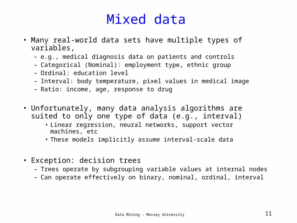
Mixed data• Many real-world data sets have multiple types of
variables, – e.g., medical diagnosis data on patients and controls– Categorical (Nominal): employment type, ethnic group– Ordinal: education level– Interval: body temperature, pixel values in medical image– Ratio: income, age, response to drug
• Unfortunately, many data analysis algorithms are suited to only one type of data (e.g., interval)
• Linear regression, neural networks, support vector machines, etc
• These models implicitly assume interval-scale data
• Exception: decision trees– Trees operate by subgrouping variable values at internal nodes– Can operate effectively on binary, nominal, ordinal, interval
Data Mining - Massey University 12
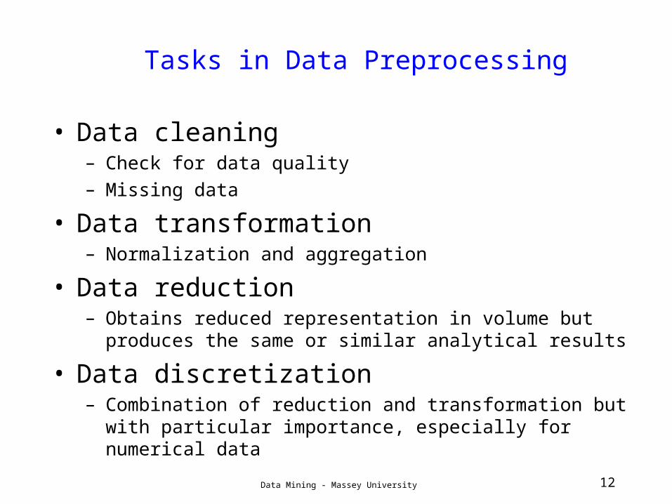
Tasks in Data Preprocessing
• Data cleaning– Check for data quality– Missing data
• Data transformation– Normalization and aggregation
• Data reduction– Obtains reduced representation in volume but
produces the same or similar analytical results
• Data discretization– Combination of reduction and transformation but with
particular importance, especially for numerical data

Data Mining - Massey University 13
Data Cleaning / Quality
• Individual measurements– Random noise in individual measurements
• Outliers• Random data entry errors• Noise in label assignment (e.g., class labels in medical data sets)• can be corrected or smoothed out
– Systematic errors• E.g., all ages > 99 recorded as 99• More individuals aged 20, 30, 40, etc than expected
– Missing information• Missing at random
– Questions on a questionnaire that people randomly forget to fill in• Missing systematically
– Questions that people don’t want to answer– Patients who are too ill for a certain test

Data Mining - Massey University 14
Missing Data
• Data is not always available– E.g., many records have no recorded value for several
attributes,
• survey respondents
• disparate sources of data
• Missing data may be due to – equipment malfunction
– inconsistent with other recorded data and thus deleted
– data not entered due to misunderstanding
– certain data may not be considered important at the time of entry
– not register history or changes of the data

Data Mining - Massey University 15
How to Handle Missing Data?
• Ignore the tuple: not effective when the percentage
of missing values per attribute varies considerably.
• Fill in the missing value manually: tedious +
infeasible?
• Use a global constant to fill in the missing value: e.g.,
“unknown”, a new class?!
• Use the attribute mean to fill in the missing value
• Use imputation
– nearest neighbor
– model based (regression or Bayesian MC based)
Data Mining - Massey University 16
Missing Data
• What do I choose for a given situation?
• What you do depends
– the data - how much is missing? are they
‘important’ values?
– the model - can it handle missing values?
– there is no right answer!
Data Mining - Massey University 17
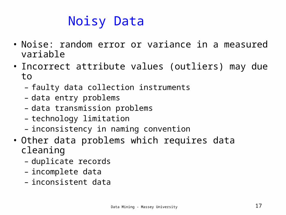
Noisy Data
• Noise: random error or variance in a measured variable
• Incorrect attribute values (outliers) may due to– faulty data collection instruments– data entry problems– data transmission problems– technology limitation– inconsistency in naming convention
• Other data problems which requires data cleaning– duplicate records– incomplete data– inconsistent data

Data Mining - Massey University 18
How to Handle Noisy Data?
• Is the suspected outlier from– human error? or– real data?
• err on the side of caution, if unsure, use methods that are robust to outliers

Data Mining - Massey University 19
Data Transformation
• Can help reduce influence of extreme values
• Putting data on the real line is often convenient
• Variance reduction:– log-transform often used for incomes and other highly
skewed variables.
• Normalization: scaled to fall within a small, specified range– min-max normalization
– z-score normalization
– normalization by decimal scaling
• Attribute/feature construction– New attributes constructed from the given ones

Data Mining - Massey University 20
Data Transformation: Standardization
We can standardize data by dividing by the sample standard deviation. This makes them all equally important.
( )2
1
1
21ˆ ⎟
⎠
⎞⎜⎝
⎛−= ∑
=
n
ikkk xx
nσ
The estimate for the standard deviation of xk :
where xk is the sample mean:
∑=
=n
ikk ix
nx
1
)(1
(When might standardization *not* be a such a good idea?)

Data Mining - Massey University 21
Dealing with massive data
• What if the data simply does not fit on my computer (or R crashes)?– Force the data into main memory
• be careful, you need some overhead for modelling!
– use scalable algorithms• keep up on the literature, this keeps changing!
– Use a database• Mysql is a good (and free) one
– Investigate data reduction strategies

Data Mining - Massey University 22
Data Reduction: Strategies
• Warehouse may store terabytes of data: Complex data analysis/mining may take a very long time to run on the complete data set
• Data reduction – Obtains a reduced representation of the data set
that is much smaller in volume but yet produces the same (or almost the same) analytical results
– Goal: reduce dimensionality of data from p to p’

Data Mining - Massey University 23
Data Reduction: Dimension Reduction
• In general, incurs loss of information about x
• If dimensionality p is very large (e.g., 1000’s), representing the data in a lower-dimensional space may make learning more reliable,– e.g., clustering example
• 100 dimensional data• if cluster structure is only present in 2 of the
dimensions, the others are just noise• if other 98 dimensions are just noise (relative to
cluster structure), then clusters will be much easier to discover if we just focus on the 2d space
• Dimension reduction can also provide interpretation/insight– e.g for 2d visualization purposes

Data Mining - Massey University 24
Data Reduction: Dimension Reduction
• Feature selection (i.e., attribute subset selection):– Select a minimum set of features such that the
minimal signal is lost
• Heuristic methods (exhaustive search implausible except for small p):– step-wise forward selection– step-wise backward elimination– combining forward selection and backward
elimination– decision-tree induction
• can work well, but often gets trapped in local minima
• often computationally expensive

Data Mining - Massey University 25
• One of several projection methods
• Given N data vectors from k-dimensions, find c <= k orthogonal vectors that can be best used to represent data – The original data set is reduced to one consisting of
N data vectors on c principal components (reduced dimensions)
• Each data vector is a linear combination of the c principal component vectors
• Works for numeric data only
• Used when the number of dimensions is large
Data Reduction: Principal Components

Data Mining - Massey University 26
PCA Example
Direction of 1st principal component vector (highest variance projection)
x1
x2

Data Mining - Massey University 27
PCA Example
Direction of 1st principal component vector (highest variance projection)
x1
x2
Direction of 2ndprincipal component vector

Data Mining - Massey University 28
Data Reduction: Multidimensional Scaling
• Say we have data in the form of an N x N matrix of dissimilarities– 0’s on the diagonal– Symmetric– Could either be given data in this form, or create such a
dissimilarity matrix from our data vectors
• Examples– Perceptual dissimilarity of N objects in cognitive science
experiments– String-edit distance between N protein sequences
• MDS:– Find k-dimensional coordinates for each of the N objects such that
Euclidean distances in “embedded” space matches set of dissimilarities as closely as possible

Data Mining - Massey University 29
Multidimensional Scaling (MDS)
• MDS score function (“stress”)
• Often used for visualization, e.g., k=2, 3
∑∑ −=jiji
jidjijidS,
2
,
2 ),(/)),(),(( δ
Originaldissimilarities
Euclidean distancein “embedded” k-dim space

Data Mining - Massey University 30
MDS: Example data

Data Mining - Massey University 31
MDS: 2d embedding of face images

Data Mining - Massey University 32
Data Reduction: Sampling
• Don’t forget about sampling!• Choose a representative subset of the data
– Simple random sampling may be ok but beware of skewed variables.
• Stratified sampling methods– Approximate the percentage of each
class (or subpopulation of interest) in the overall database
– Used in conjunction with skewed data– Propensity scores may be useful if
response is unbalanced.

Data Mining - Massey University 33
Data Discretization
• Discretization:
– divide the range of a continuous attribute into intervals
– Some classification algorithms only accept categorical attributes.
– Reduce data size by discretization– Prepare for further analysis
• Reduces information in the data, but sometimes surprisingly good!– Bagnall and Janacek - KDD 2004

Data Mining - Massey University 34
Model Evaluation

Data Mining - Massey University 35
Model Evaluation
• e.g. pick the “best” a and b in Y = aX + b
• how do you define “Best?”
• Big difference between Data Mining and Statistics is the focus on predictive performance over find best estimators.
• Most obvious criterion for predictive performance:
Data Mining - Massey University 36
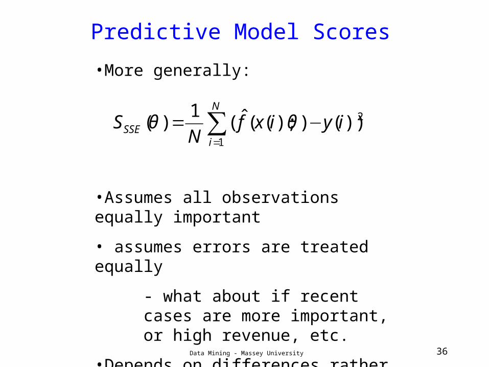
Predictive Model Scores
∑=
−=N
iSSE iyixf
NS
1
2))());((ˆ(1
)( θθ
•More generally:
•Assumes all observations equally important
• assumes errors are treated equally
- what about if recent cases are more important, or high revenue, etc.
•Depends on differences rather than values
- scale matters with squared error

Data Mining - Massey University 37
Descriptive Model Scores
∏=
=N
i
ixpL1
));((ˆ)( θθ
•If your model assigns probabilities to classes:
• likelihood based - “Pick the model that assigns highest probability to what actually happened”
• Many different scoring rules for non-probabilistic models

Data Mining - Massey University 38
Scoring Models with Different Complexities
score(model) = Goodness-of-fit - penalty for complexity
Classic bias/variance tradeoff
this is called “regularization” and is used to combat “overfitting”
complex models can fit data perfectly!!!!

Data Mining - Massey University 39
Using Hold-Out Data
• Instead of penalizing complexity, look at performance on hold-out data
• Using the same set of examples for training as well as for evaluation results in an overoptimistic evaluation of model performance.
Need to test performance on data not “seen” by the modeling algorithm. I.e., data that was no used for model building

Data Mining - Massey University 40
Data Partition
• Randomly partition data into training and test set• Training set – data used to train/build the model.
– Estimate parameters (e.g., for a linear regression), build decision tree, build artificial network, etc.
• Test set – a set of examples not used for model induction. The model’s performance is evaluated on unseen data. Also referred to as out-of-sample data.
• Generalization Error: Model’s error on the test data.
Set of training examplesSet of testexamples

Data Mining - Massey University 41
Training Data:Customer characteristics &cell phone usage behavior
Model
Model Inductionalgorithm
Set of training examples
Set of testingexamples
Use model to predict outcome on test set
The model is used to infer whether a customer would leave
ConsumerI
ModelPredictionwhether
customer I willterminatecontract

Data Mining - Massey University 4242
Holding out data
• The holdout method reserves a certain amount for testing and uses the remainder for training– Usually: one third for testing, the rest for
training
• For “unbalanced” datasets, random samples might not be representative– Few or none instances of some classes
• Stratified sample: – Make sure that each class is represented with
approximately equal proportions in both subsets

Data Mining - Massey University 4343
Evaluation on “small” data
• What if we have a small data set?• The chosen 2/3 for training may
not be representative.• The chosen 1/3 for testing may not
be representative.

Data Mining - Massey University 4444
Repeated holdout method
• Holdout estimate can be made more reliable by repeating the process with different subsamples– In each iteration, a certain proportion is
randomly selected for training (possibly with stratification)
– The error rates on the different iterations are averaged to yield an overall error rate
• This is called the repeated holdout method

Data Mining - Massey University 4545
Cross-validation
• Most popular and effective type of repeated holdout is cross-validation
• Cross-validation avoids overlapping test sets– First step: data is split into k subsets of equal
size– Second step: each subset in turn is used for
testing and the remainder for training
• This is called k-fold cross-validation• Often the subsets are stratified before the
cross-validation is performed• The error estimates are averaged to yield
an overall error estimate

Data Mining - Massey University 4646 46
Cross-validation example:
— Break up data into groups of the same size —
—
— Hold aside one group for testing and use the rest to build model
—
— Repeat
Test

Data Mining - Massey University 4747
More on cross-validation
• Standard method for evaluation: stratified ten-fold cross-validation
• Why ten? Extensive experiments have shown that this is the best choice to get an accurate estimate
• Stratification reduces the estimate’s variance
• Even better: repeated stratified cross-validation– E.g. ten-fold cross-validation is repeated ten
times and results are averaged (reduces the variance)

Data Mining - Massey University 4848
Leave-One-Out cross-validation
• Leave-One-Out:a particular form of cross-validation:– Set number of folds to number of training
instances– I.e., for n training instances, build classifier n
times
• Makes best use of the data• Involves no random subsampling • Computationally expensive, but good
performance

Data Mining - Massey University 4949
Leave-One-Out-CV and stratification
• Disadvantage of Leave-One-Out-CV: stratification is not possible– It guarantees a non-stratified sample because
there is only one instance in the test set!
• Extreme example: random dataset split equally into two classes– Best model predicts majority class– 50% accuracy on fresh data – Leave-One-Out-CV estimate is 100% error!

Data Mining - Massey University 50
Model’s Performance Evaluation
Classification models predict what class an observation belongs to.E.g., good vs. bad credit risk (Credit), Response
vs. no response to a direct marketing campaign, etc.
Classification Accuracy RateProportion of accurate classifications of examples in test set. E.g., the model predicts the correct class for 70% of test examples.

Data Mining - Massey University 51
Classification Accuracy Rate
Classification Accuracy Rate: S/N = Proportion examples accurately classified by the model
S – number of examples accurately classified by modelN – Total number of examples
Inputs Output Model’s prediction
Correct/incorrect prediction
Single No of cards
Age Income>50K Good/Bad risk
Good/Bad risk
0 1 28 1 1 1 :)
1 2 56 0 0 0 :)
0 5 61 1 0 1 :(
0 1 28 1 1 1 :)
… … … … … … …

Data Mining - Massey University 52
Consider the following…
• Response rate for a mailing campaign is 1%• We build a classification model to predict
whether or not a customer would respond.• The model classification accuracy rate is
99%• Is the model good?
99% do not respond1%
respond

Data Mining - Massey University 53
Respond Do not respond
Respond 0 0
Do not Respond
10 990
Diagonal left to right: predicted class=actual class. 990/1000 (99%) accurate predictions.
Model’s performance over test set:
Predicted Class
Actual Class
Confusion Matrix for Classification

Data Mining - Massey University 54
Evaluation for a Continuous Response
• In a logistic regression example, we predict probabilites that the response = 1.
• Classification accuracy depends on the threshold

Data Mining - Massey University 55
Test Data
predicted probabilities
8 3
0 9
1
0
01
actual outcome
predictedoutcome
Suppose we use a cutoff of 0.5…

Data Mining - Massey University 56
a b
c d
1
0
01
actual outcome
predictedoutcome
More generally…
misclassification rate: b + c
a+b+c+d
recall or sensitivity (how many of those that are really positive did you predict?):
a
a+c
specificity: d
b+d
precision (how many of those predicted positive really are?)
a
a+b

Data Mining - Massey University 57
8 3
0 9
1
0
01
actual outcome
predictedoutcome
Suppose we use a cutoff of 0.5…
sensitivity: = 100% 8
8+0
specificity: = 75% 9
9+3
we want both of these to be high

Data Mining - Massey University 58
6 2
2 10
1
0
01
actual outcome
predictedoutcome
Suppose we use a cutoff of 0.8…
sensitivity: = 75% 6
6+2
specificity: = 83% 10
10+2

Data Mining - Massey University 59
• Note there are 20 possible thresholds
• ROC computes sensitivity and specificity for all possible thresholds and plots them
• Note if threshold = minimum
c=d=0 so sens=1; spec=0
• If threshold = maximum
a=b=0 so sens=0; spec=1
a b
c d
1
0
01
actual outcome

Data Mining - Massey University 60
“Area under the curve” (AUC) is a common measure of predictive performance

Data Mining - Massey University 61
Another Look at ROC Curves
Test Result
Pts Pts with with diseasdiseasee
Pts Pts without without the the diseasedisease

Data Mining - Massey University 62
Test Result
Call these patients “negative”
Call these patients “positive”
Threshold

Data Mining - Massey University 63
Test Result
Call these patients “negative”
Call these patients “positive”
without the diseasewith the disease
True Positives
Some definitions ...

Data Mining - Massey University 64
Test Result
Call these patients “negative”
Call these patients “positive”
without the diseasewith the disease
False Positives

Data Mining - Massey University 65
Test Result
Call these patients “negative”
Call these patients “positive”
without the diseasewith the disease
True negatives
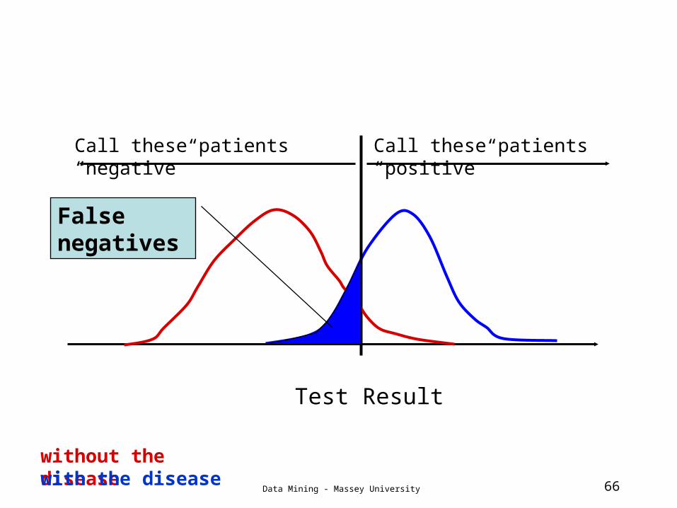
Data Mining - Massey University 66
Test Result
Call these patients “negative”
Call these patients “positive”
without the diseasewith the disease
False negatives

Data Mining - Massey University 67
Test Result
without the diseasewith the disease
‘‘‘‘-’-’’’
‘‘‘‘+’+’’’
Moving the Threshold: right

Data Mining - Massey University 68
Test Result
without the diseasewith the disease
‘‘‘‘-’-’’’
‘‘‘‘+’+’’’
Moving the Threshold: left

Data Mining - Massey University 69
Tru
e P
osi
tive R
ate
(s
en
siti
vit
y)
0%
100%
False Positive Rate (1-specificity)
0%
100%
ROC curve

Data Mining - Massey University 70
Tru
e P
osi
tive
Rate
0%
100%
False Positive Rate
0%
100%
Tru
e P
osi
tive
Rate
0%
100%
False Positive Rate
0%
100%
A good test: A poor test:
ROC curve comparison
Data Mining - Massey University 71
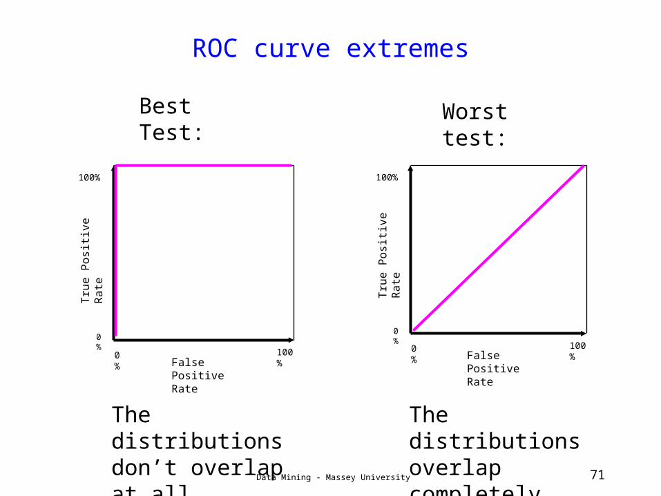
Best Test: Worst test:T
rue P
osi
tive
R
ate
0%
100%
False Positive Rate
0%
100%
Tru
e P
osi
tive
R
ate
0%
100%
False Positive Rate
0%
100%
The distributions don’t overlap at all
The distributions overlap completely
ROC curve extremes

Data Mining - Massey University 72
ROC Curve
Ideal ROC curve (AUC=1)
100%
100%
0 AUC 1
Actual R
OC
Random ROC
(AUC=0.5)
0
For a given threshold on f(x), you get a point on the ROC curve.
Positive class success rate
(hit rate, sensitivity)
1 - negative class success rate (false alarm rate, 1-specificity)

Data Mining - Massey University 73
Tru
e P
osi
tive
R
ate
0%
100%
False Positive Rate
0%
100%
Tru
e P
osi
tive
R
ate
0%
100%
False Positive Rate
0%
100%
Tru
e P
osi
tive
R
ate
0%
100%
False Positive Rate
0%
100%
AUC = 50%
AUC = 90% AUC =
65%
AUC = 100%
Tru
e P
osi
tive
R
ate
0%
100%
False Positive Rate
0%
100%
AUC for ROC curves

Data Mining - Massey University 74
Interpretation of AUC
• AUC can be interpreted as the probability that the test result from a randomly chosen diseased individual is more indicative of disease than that from a randomly chosen nondiseased individual: P(Xi Xj | Di = 1, Dj = 0)
• So can think of this as a nonparametric distance between disease/nondisease test results
• equivalent to Mann-Whitney U-statistic (nonparametric test of difference in location between two populations)

Data Mining - Massey University 75
Lab #3
• Missing Data: using visualization to see if the data is missing at random through “missing in the margins”
• Multi-dimensional scaling