data modeling · disadvantages of mpp columnar stores 8 ... teradata aster data, paraccel analytic...

1A SApient CASe Study © SApient CorporAtion 2014

DATA MODELINGApplying Relevant Data Modeling Techniques to MPP Columnar Stores - A Point of View

Author: Sudershan Srinivasan

FINANCE 1

FINANCE 2

FINANCE 3

FINANCE 4

FINANCE 1

FINANCE 2

FINANCE 3

FINANCE 4

http://www.sapient.com/en-us/global-markets.html

2Applying RelevAnt DAtA MoDeling techniques to Mpp coluMnAR stoRes: A Point of View

Contents

Introduction 3

Executive Summary 3

MPP Columnar Database Architecture 4

Columnar Storage 5

Key Advantages of MPP Columnar Stores 7

Disadvantages of MPP Columnar Stores 8

Use Cases for MPP Columnar Stores 8

Applying Relevant Data Modeling Techniques to MPP Columnar Stores 9

1. Defining the Grain 9

2. Data Distribution and Co-Location – Key Concepts 10

2a. Data Co-Location with Single and Multiple Columns 12

3. Flattening the Data Model/Minimizing Joins 14 Between Extremely Heavy Tables

4. Managing Facts 16

5. Managing Dimensions 17

6. Handling DMLs (Insert, Update, Delete Operations) 21

7. Handling DMLs (Insert, Update, Delete Operations) 22

MPP Columnar Stores and Big Data Architecture 24

Conclusions 26

References & Acknowledgements 27

Appendix 28

Data Accessibility 28

Quick Primer on Slowly Changing Dimensions 29

Quick Primer on Facts and Fact Types 32


Today, every organization wants to do detailed analysis of data, to do it faster and to analyze ever-increasing amounts of data.

Traditional row-based data warehouse systems are unable to scale and cater to this growing demand to accommodate more data without compromising performance.

In terms of total cost of ownership, return on investment (ROI), time to market, performance and scalability, Massively Parallel Processing (MPP) columnar stores have significant advantages# over both traditional row-based data warehouse systems and data warehouse appliances. As a result, MPP columnar stores are gaining faster adoption and acceptance.*

Popular MPP columnar stores include HP Vertica, EMC Greenplum, Teradata Aster Data, ParAccel Analytic DB and Calpont, to name a few.

Industry experts today acknowledge that map-reduce/Hadoop solutions will coexist with high-performing data warehouse solutions—enabling better, more holistic insight by filtering information from unstructured data and joining it with various dimensions in the corporate data warehouse.

In this way, MPP columnar stores are also bridging the worlds of structured and unstructured data.

This point-of-view document brings into focus MPP columnar stores, covers the architecture of MPP and columnar store databases, enlists key advantages (and a few disadvantages), outlines relevant data modeling techniques and shows how they fit in the world of Big Data.

The document explores the question: With MPP columnar stores, would traditional data models (dimensional models/star schema), typically used for analytics, still be relevant? Or are there more optimal, less rigid data models that MPP columnar stores enable?

The following assumptions are relevant to this document:

• Not all MPP products are columnar, but in this document we are considering products that are both MPP and columnar.

• New modeling techniques have not been defined in this document. The document merely shows which techniques are more suited or need to be modified in the context of MPP columnar stores.

IntRoDUCtIon

eXeCUtIVe sUMMARY

# Click here to see › Comparison of MPP solutions with Data Warehouse Appliance * Click here to see › Gartner’s Magic Quadrant for Data Warehouse.

http://wikibon.org/wiki/v/Financial_Comparison_of_Big_Data_MPP_Solution_and_Data_Warehouse_Appliance

http://www.odbms.org/2014/03/2014-gartner-magic-quadrant-data-warehouse-database-management-systems/


MPP architecture employs massively parallel processing to allow data ingestion/loading and data processing/querying on multiple machines simultaneously. Although this architecture has been around for a long time, it has recently returned to the limelight thanks to the need to analyze huge data sets.

Systems based on MPP architecture typically consist of a master node, a group of compute nodes and a network fabric (pvt. n/w) for intercommunication between the nodes. Aside from those characteristics, MPP systems typically have specialized algorithms to completely parse all queries, divide the workload between the available compute nodes and work in parallel on distributed data (which may run into petabytes).

Unlike data warehouse appliances (which have “Shared Everything” architecture), MPP systems are typically “Shared Nothing” architecture (see Figure 1 for the MPP architecture that can be generalized to many MPP offerings).

The master node:

• Interacts with the clients

• Distributes workload among the compute nodes

• Parses the queries and generates the execution plan

• Keeps track of data distribution

• Aggregates intermediate results from the nodes and stitches them together before sending to the client

The compute nodes store and compute data locally. The compute nodes cannot be accessed directly; all client interactions are handled by the Master node.

Network, or interconnect, fabric is a private network between all the compute nodes and the master node. This is an optimized network with high bandwidth and high redundancy.

MPP ColUMnAR DAtAbAse ARChIteCtURe

Figure 1. MPP architecture depicting the master node, network fabric and compute nodes.

Interconnect Fabric

Master node

Compute node

5A sAPIent CAse stUDY © sAPIent CoRPoRAtIon 2013

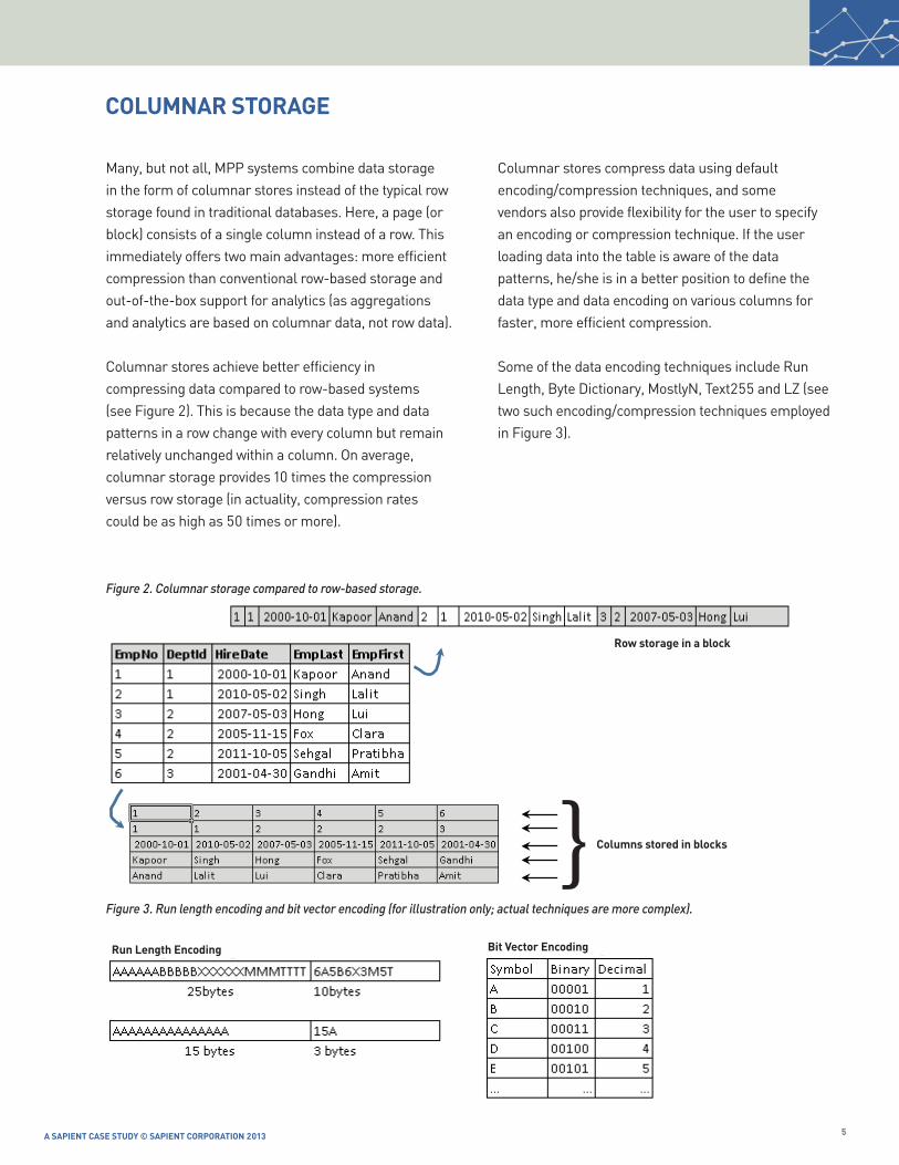
Many, but not all, MPP systems combine data storage in the form of columnar stores instead of the typical row storage found in traditional databases. Here, a page (or block) consists of a single column instead of a row. This immediately offers two main advantages: more efficient compression than conventional row-based storage and out-of-the-box support for analytics (as aggregations and analytics are based on columnar data, not row data).

Columnar stores achieve better efficiency in compressing data compared to row-based systems (see Figure 2). This is because the data type and data patterns in a row change with every column but remain relatively unchanged within a column. On average, columnar storage provides 10 times the compression versus row storage (in actuality, compression rates could be as high as 50 times or more).

Columnar stores compress data using default encoding/compression techniques, and some vendors also provide flexibility for the user to specify an encoding or compression technique. If the user loading data into the table is aware of the data patterns, he/she is in a better position to define the data type and data encoding on various columns for faster, more efficient compression.

Some of the data encoding techniques include Run Length, Byte Dictionary, MostlyN, Text255 and LZ (see two such encoding/compression techniques employed in Figure 3).

ColUMnAR stoRAge

Figure 2. Columnar storage compared to row-based storage.

Figure 3. Run length encoding and bit vector encoding (for illustration only; actual techniques are more complex).

Row storage in a block

Columns stored in blocks

bit Vector encodingRun length encoding

}


Traditional row-oriented databases employ indexes or materialized views to quickly access the underlying table data. This is not needed in columnar databases since each column itself acts as a bit map index. Thus, columnar databases do not have a need for indexes, materialized views or index-organized tables—greatly reducing the operational effort to create and maintain these performance-tuning objects.

These advanced data compression and encoding techniques, as well as data de-duplication methods, yield astonishing query response speed in columnar stores. Consequently, columnar stores do not need structures, such as indexes or materialized views, which are difficult to maintain and occupy further storage space.

In traditional row storage databases, the size of the rows in a table directly affects the performance of any SQL request targeting that table. This is because in a row-oriented database, each time the RDBMS needs to access a specific column, the full row gets accessed, as the level of I/O operation is the entire record. By contrast, with columnar storage the level of I/O operation is the column and not the row. In data warehouse applications, columns (not rows) are important. With an analytical query—whether computations like AVG, SUM or MAX—drilling across multiple columns, there is never a need to access the entire row. Only the specific columns are required, drastically reducing I/O. Column stores thus aid analytical queries by extracting only the required columns.

ColUMnAR stoRAge (Continued)

Figure 4. Performance of analytical queries in row-oriented databases versus columnar stores.

SELECT EmpLast, EmpFirst from Employee_Dim -- oldest employee in Org.

WHERE HireDate IN (Select MIN(HireDate) from Employee_Dim);

Index Access + table Row Access

+X

only Column Access


also support on-the-fly transformations and aggregations thanks to their high processing capabilities and efficient interconnect algorithms.

• Ability to simply load and analyze. One can not only query but also load data into MPP columnar stores with great speed and efficiency. Terabytes of data in flat files can be loaded in minutes and with minimal effort. After the data is loaded, one does not need to create any other database objects (such as views, indexes or stats update) to access and analyze this data. Data can be queried immediately.

• support for commodity hardware. Not all MPP columnar stores are built on proprietary hardware. Use of commodity hardware helps reduce overall costs without compromising performance or scalability. The only advantage that some of the proprietary hardware MPP solutions provide is tight coupling of the hardware to some of the algorithms for storing, processing and querying data.

• Cloud support. MPP columnar stores can be deployed in the cloud, further reducing infrastructure maintenance costs and easing on-the-fly scalability.

• In-memory support. MPP columnar stores also have in-memory capabilities and implementations.

• Integration with other big Data processing technologies. MPP columnar stores today have efficient adaptors that integrate with other Big Data processing technologies, such as Hadoop/NoSQL, which have proven their ability to quickly process unstructured data. This integration capability is helping organizations to realize the full potential of MPP columnar stores.

• Reduced time to value or market. Due to their relatively low cost of ownership, lower administration/maintenance and high performance, MPP columnar stores help accelerate overall time to value or time to market.

MPP columnar stores offer these key advantages:

• Massive processing. MPP systems bring in massive processing power to work with petabytes of data while returning results in a fraction of the time required in a typical RDBMS. It does this through parallel processing (that is, workload distributed across compute nodes and then aggregated at the master node).

• no single point of failure. MPP columnar stores have “shared nothing” architecture, which ensures there is no single point of failure. Each node operates independently of the others, so if one machine fails, the others keep running. Even the roles of the master node can fail over or be promoted to a compute node. The results: redundancy and high availability.

• scalability. Again, thanks to the “shared nothing” approach, MPP columnar stores provide linear scalability with the addition of more hardware (that is, compute nodes). Due to system bus limitations in traditional systems, increasing the hardware resource does not lead to linear scalability.

• Petabyte scale support. Thanks to compression, encoding and distribution of data across nodes, MPP columnar systems support data volumes to petabytes and even exabytes of data.

• Divide and conquer method. MPP systems use the “divide and conquer” method to manage data volumes. Data is distributed across all the nodes, with each node processing its own (local) data when a query is fired. This dramatically improves query performance—sometimes to the tune of 100 times versus traditional RDBMS.

• Advanced compression. MPP columnar stores bring in advanced and highly efficient compression methods as compared to traditional row-based database systems. Data encoding, a technique related to compression, allows both efficient storage and retrieval of data with fewer hardware resources.

• native analytics. MPP columnar stores support native analytics, which ease aggregation and analytical capabilities. Some MPP columnar stores

KeY ADVAntAges oF MPP ColUMnAR stoRes


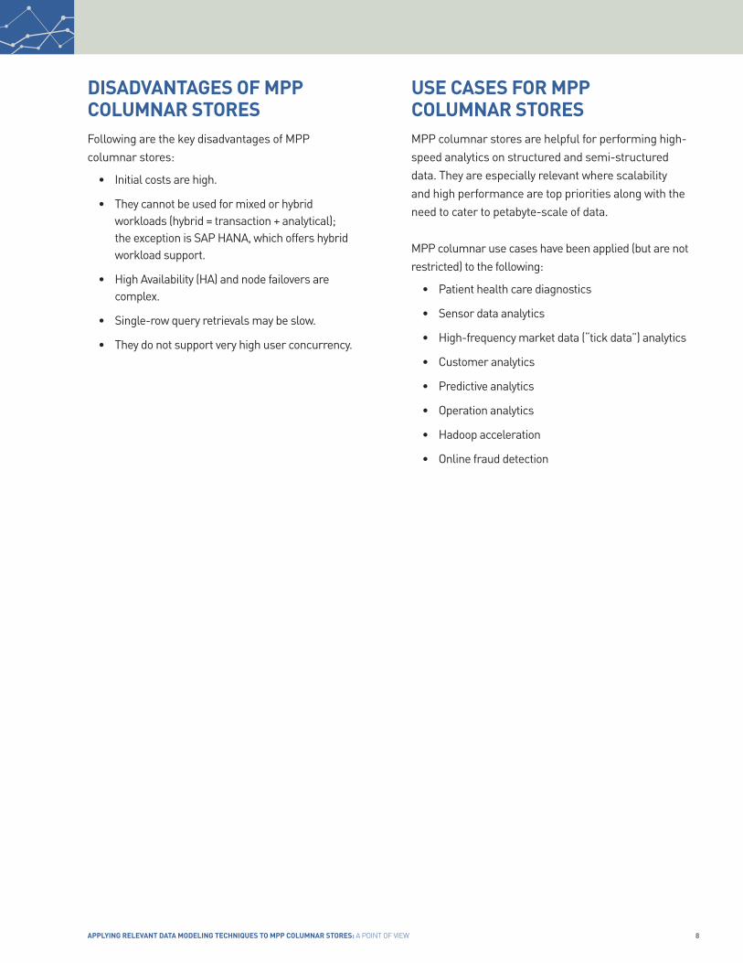
MPP columnar stores are helpful for performing high-speed analytics on structured and semi-structured data. They are especially relevant where scalability and high performance are top priorities along with the need to cater to petabyte-scale of data.

MPP columnar use cases have been applied (but are not restricted) to the following:

• Patient health care diagnostics

• Sensor data analytics

• High-frequency market data (“tick data”) analytics

• Customer analytics

• Predictive analytics

• Operation analytics

• Hadoop acceleration

• Online fraud detection

Following are the key disadvantages of MPP columnar stores:

• Initial costs are high.

• They cannot be used for mixed or hybrid workloads (hybrid = transaction + analytical); the exception is SAP HANA, which offers hybrid workload support.

• High Availability (HA) and node failovers are complex.

• Single-row query retrievals may be slow.

• They do not support very high user concurrency.

DIsADVAntAges oF MPP ColUMnAR stoRes

Use CAses FoR MPP ColUMnAR stoRes


Because MPP columnar stores cater to analytics, most of the data warehousing modeling techniques also apply.

OLTP databases have their own space for transactional applications and MPP columnar stores do not replace transactional OLTP systems.

1. DeFInIng the gRAInA coarse grain declaration – “Sum of Sales for a state”versusA detailed grain declaration – “Sales detail of retail stores across all cities of a state for a month”

Clearly, the grain:

• Directly affects the volume of data that the data warehouse stores

• Affects the types of queries that can be posed and answered

Pros1. Coarse granularity (aggregation) helps in

drastically reducing data content—saving on storage and improving overall performance for processing, query retrieval and backups/archival.

2. Fine granularity helps address future ad-hoc/unknown queries and requirements and supports deeper analysis.

Cons1. With coarse graining, some business questions

cannot be answered as the data for the same is not available in the warehouse.

2. Fine graining obviously increases storage costs and affects performance.

In MPP columnar stores, it is advisable to have fine-grained facts as one need not worry about the enormity of data or performance.

APPlYIng ReleVAnt DAtA MoDelIng teChnIqUes to MPP ColUMnAR stoRes

Figure 5. An example illustrating the concept of granularity in data modeling.

Coarse grained

Sum of Sales for a State

1 Row

x 25 business days

x 68 bytes = 1.6 Kb in a month

✔ Which date had the highest sales for the month? ✔ Which date had the highest sales for the month?

✔ List out Retail Stores having the maximum sales - by city?

100,000 Rows

x 25 business days

x 142 bytes = 338.5 Mb in a month

Fine grained

Sales details of Retail Stores across all cities of a State

Column name type bytes

Sales_Date date 10

State varchar(50) 50

Sum_Sales_Qty float 16

Column name type bytes

Sales_Date date 10

Sales_Time timestamp 8

Retail_Store_Id int 8

City varchar(50) 50

State varchar(50) 50

Sales_Qty Float 16


Figure 6 depicts that the data of the “Products” table has been distributed on the ProductId. We execute the following queries:

Query A – SELECT * FROM products p WHERE p.productId = 5;

Query B – SELECT * FROM products p WHERE p.productId in (1, 3);

For query A, the master node will parse and generate the query plan and will then issue the query to node 2 as it is aware of the data distribution of the table. Now the query needs to scan only three rows in node 2 as compared to nine rows if the table were not distributed in a typical RDBMS.

For query b, the query is submitted to node 1 and node 3 in parallel. Each parallel process will scan only three rows and return the datasets back to the master node. The master node will then stitch the results together and return the result to the end user.

2. DAtA DIstRIbUtIon AnD Co-loCAtIon – KeY ConCePts

Data distribution is a physical modeling concept, but a discussion of the same is relevant. The design of the tables and the choice of the distribution key are data modeling decisions that directly impact the physical distribution of data in the MPP cluster. This can have significant impact on the performance of the system.

In MPP columnar stores, one may specify how data is distributed to the compute nodes or allow the MPP columnar database to handle distribution. Hashing techniques or “Round Robin” methods are used for distribution (see Figure 6).

APPlYIng ReleVAnt DAtA MoDelIng teChnIqUes to MPP ColUMnAR stoRes (Continued)

Figure 6. data distribution in an MPP columnar store.

query A:

SELECT * FROM products p

WHERE p.productId = 5;

query b:

SELECT * FROM products p

WHERE p.productId IN (1,3);

Client Master/Leader Node

Compute Node1

Compute Node2

Compute Node3

1 samsung galaxy s4

4 Apple iPhone 5s

7 htC one

2 sony Xperia Z1

5 lg g2

8 nokia lumia 1525

3 blackberry Z10

6 Motorolla Moto X

9 lenovo Vibe Z


best Practices for choosing the distribution key:

• Unique (primary) keys are preferred.

• Explicitly define a column as the DistKey. Otherwise, the first column may be used for distribution by default.

• For frequently joined tables, use the same column as the DistKey. This would promote co-location that greatly improves performance.

• When data is co-located during a join operation, data from the compute nodes are processed locally without the need for data to travel, or broadcast, to other nodes. In other words, data co-location is a good thing.

• Try a distribution key such that query processing workload can be distributed across nodes as much as possible with minimal data transfer across the nodes. Columns “most generally” used for filtering (for example, the date column) are not good distribution key candidates. Those columns will localize query processing instead of utilizing all the compute nodes.

• Dictionary tables are available to see how the distribution has taken place. They help in analyzing skew-ness, taking corrective actions on data distribution and improving performance.

Despite all the points above, not all queries can be distributed or co-located. Even then, however, MPP columnar stores help.

Pros1. Data distribution helps distribute query processing

across the compute nodes, resulting in faster response as long as data movement across the nodes is minimal during join operations.

2. Distribution also helps in retrieving data by skipping nodes and scanning fewer rows to obtain the final result set—thereby improving performance.

Cons1. Changing a data distribution key is not simple; it

means the entire table must be recreated (requiring backing up the table, creating a new table with a new distribution key, copying/loading data to the new table, reorganizing data as per new DistKey and dropping the older table).

2. Most MPP columnar stores allow distribution only on a single column (not a group of columns) with the sole exception being Teradata. A workaround could be the creation of a custom column having concatenated values from multiple columns (see Figure 8).

3. Improper choice of DistKey could lead to process and data skews, resulting in poor performance. For example, using the gender column (male/female) as a distribution key could potentially cause half of the nodes to remain idle. Improper DistKeys could also cause excessive data transfers across the nodes, resulting in suboptimal performance.

4. It is not always easy or feasible to declare the same column as the distribution key in two tables and also gain the advantage of co-location:

• Various columns can be used as join keys, but only one can be used as a distribution key.

• The join key and distribution key could be different.

• Join keys change from query to query.

• A workaround is to use custom columns having concatenated values as the DistKey (see Figure 8).



The situation worsens when DistKey is different on two tables and join happens on neither of the DistKeys. DistKey can be created only during table creation, and one cannot alter it as per query requirements. With the sole exception of Teradata (Aster Database), most MPP columnar stores allow only one column to be used as DistKey. That means that one may not always be able to benefit from data co-location because different queries have different join conditions. The workaround is to create a custom DistKey with concatenated values from the join columns, as illustrated in the following example:

• If the MPP columnar product does not support distribution on more than one column, there is a workaround.

• This prompts the need to create a new column with concatenated values from the required (join) columns.

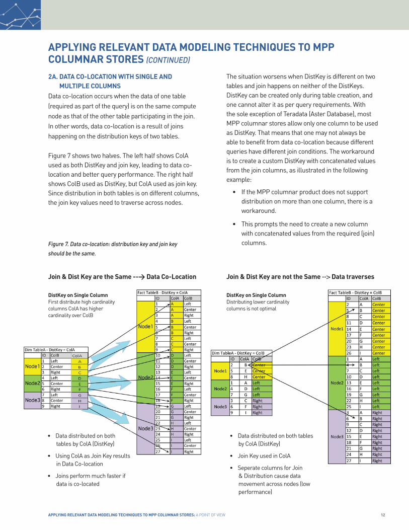
2A. DAtA Co-loCAtIon wIth sIngle AnD MUltIPle ColUMns

Data co-location occurs when the data of one table (required as part of the query) is on the same compute node as that of the other table participating in the join. In other words, data co-location is a result of joins happening on the distribution keys of two tables.

Figure 7 shows two halves. The left half shows ColA used as both DistKey and join key, leading to data co-location and better query performance. The right half shows ColB used as DistKey, but ColA used as join key. Since distribution in both tables is on different columns, the join key values need to traverse across nodes.

Figure 7. data co-location: distribution key and join key

should be the same.


DistKey on single ColumnFirst distribute high cardinality columns ColA has higher cardinality over ColB

DistKey on single ColumnDistributing lower cardinality columns is not optimal

• Data distributed on both tables by ColA (DistKey)

• Using ColA as Join Key results in Data Co-location

• Joins perform much faster if data is co-located

• Data distributed on both tables by ColA (DistKey)

• Join Key used in ColA

• Seperate columns for Join & Distribution cause data movement across nodes (low performance)

Join & Dist Key are the same --> Data Co-location Join & Dist Key are not the same --> Data traverses


• If most queries use ColA and ColB (TableA) to join with ColC & ColD (of TableB), then concatenate them.

• It does not matter how the two columns are concatenated; what is critical is ensuring that both tables are concatenated in the same way (that is, you can merge ColA and ColB --> Col_AB or ColB with ColA --> Col_BA).

• Create DistKey on the new custom column (Col_AB on TableA and Col_CD on TableB).

Pros1. Creating a distribution key on a column having

concatenated values from different join columns provides a way of gaining the advantages of co-location. These advantages can prove significant.

2. This method is particularly useful when join happens on more than one set of columns.

Cons1. It is difficult to maintain a concatenated column.

The complexity increases when more columns are merged to form a newer column.

2. Skewed distribution may happen due to newer values generated in the concatenated column. This may be counterproductive.

Key takeaway:• Before finalizing the distribution key (be it on a single

column or multiple columns), always perform tests to evaluate the ground realities.

• Unique columns (higher cardinality) are better candidates for distribution.

• At times, it may be better to have no distribution and leave the MPP columnar store to use its default means to distribute data.

• This is just a workaround; having single columns as DistKeys is simpler and preferred.

Figure 8. distribution on Col_AB and Col_Cd (or vice versa)

having concatenated values from the respective columns.

Combining values of 2 columns into a single column is one way of using multiple columns as DistKey

ColC + ColD = Col_CD

Join & Dist Key are not the same --> Data traverses

ColA + ColB = Col_AB


On the left side of Figure 9, the Fact_Table is distributed on colJ, and the Dimension table is distributed on colA.There are four nodes in the cluster. A query with a join on the two tables on colA causes data to traverse via the interconnect.

In the middle, the Fact_Table is distributed on colA, and the Dimension table is also distributed on colA. There are four nodes in the cluster. A query with a join on the two tables on column colA causes co-location; only three values traverse via interconnect for the join, which is much cleaner and faster. This is better than the previous case.

Extending the same example, if we denormalize the fact table, include colB in Fact_Table and compress colB, there would be no need for joins. This is the best case.

3. FlAttenIng the DAtA MoDel/MInIMIZIng JoIns between eXtReMelY heAVY tAbles

Analytical and data warehouse databases usually have denormalized tables. By contrast, MPP columnar stores prefer the simpler approach of flat tables. Traditional data warehouses model data in terms of facts and dimension and use the star join effectively. MPP columnar stores are schema agnostic and do not have special considerations for a star schema.

Even though MPP columnar databases support petabyte scale of data by distributing it across its compute nodes, queries with complex and heavy join operations may not return quickly. This is especially true when a join happens between two very large tables having different distribution keys. Thus, the focus in MPP columnar stores is to have flattened tables (by having dimensional data and facts together) unless the dimension is an SCD.

Let’s visualize this with an example.


Figure 9. Progressing from better to best with data co-location followed by flat structure (no joins needed).


Avoid heavy joins (that is, joins between extremely heavy tables) at all costs. Heavy joins choke the interconnect bandwidth and further affect performance for other concurrent sessions, jobs or queries.

Employ other techniques—such as redefining the grain, compressing data or improving data relevancy based on accessibility—to reduce the number of tables or the amount of data being captured into facts and dimensions.

Pros of flattening tables:1. MPP columnar stores support innumerable columns in

tables.2. Compression of columns having repeating values is a

must to save disk space and I/O.3. Flattening helps reduce efforts in designing complex

facts and dimensions. 4. Flattening helps reduce efforts in designing/developing

associated ETL jobs.5. Flattening helps reduce time to market when enterprise

design/modeling is not complete.

Cons of flattening tables:1. Flattening works in some but not all scenarios. 2. Flattening may not be scalable; one cannot continually

add more columns to a single flat table as business needs change.

normalizing Data as opposed to Flattening or De-normalizingMany MPP columnar database products are known to be “schema agnostic”—meaning that the performance of the system will be more or less the same regardless of how the tables in the schema have been modeled. There are many MPP columnar databases that support hundreds of join operations. Normalizing data increases join operations on one hand but reduces data redundancy on the other. It also provides flexibility to implement business changes without affecting the whole system.

› One needs to evaluate the tradeoffs between normalizing (number of joins) versus flattening (flexibility). Often this leads to many modelers implementing a hybrid model (taking advantage of both).

Figure 10. de-normalizing the table.


• Use compression for fact tables. Because MPP columnar stores use advanced compression techniques, these should be put to use on fine-grained facts.

• Consolidate facts. Facts should be consolidated from all available source systems. Facts should not be created as per the source type.

• Avoid centipede facts. A centipede schema is a special case of star schema in which a central fact is surrounded by several small dimensions. The resulting structure has multiple “legs” resembling a centipede (see Figure 11). Avoid centipede facts in MPP columnar stores. Centipede facts should be flattened by including the attributes of the smaller dimension in the fact table itself. This removes the need for the foreign key and the resulting join. MPP columnar stores support innumerable columns—freely expanding them to include dimensional columns.

See the Appendix for a quick primer on facts and various fact types.

4. MAnAgIng FACts

Facts are a set of measures—for example, sales revenues for a product in a quarter. Fact tables form the center of a star schema and are surrounded by dimensions associated with them as foreign keys.

Fact tables typically have millions of rows. With fewer columns but a huge number of records, they are long and skinny tables. The number of rows in a fact is directly associated to the grain that is defined. For MPP columnar stores, the traditional dimensional modeling rules can be modified.

here are a few techniques for modeling facts relevant for MPP columnar stores:

• Create the finest grains possible. With the lowest grain, aggregations are always possible, but the reverse is not. Since business users’ needs and queries change and evolve with time, modeling the lowest grain is the best. In MPP columnar stores, I/O and data size is not an issue, aiding the purpose of building out finer grains. Avoid representing facts solely as aggregates as they reduce flexibility (aggregates cannot be sliced/diced across all dimensions).

• Be consistent with the grain. Ensure that all the measures and dimensions stay consistent to the defined grain. Numeric measurements that violate the grain should not be included. In a PeriodicSnapshot, if the grain is “Month,” then one cannot include a Daily_Debit/Daily_Credit column whose grain is a “Day.” These should be computed by the business intelligence tools. Similarly, non-additive facts—such as product price in a grocery store example—should not be included in the fact itself. Price should be included in the product dimension and can serve as a slow-changing dimension.


Figure 11. A centipede fact table surrounded by several

small dimension tables.

CentiPede FactDim01(FK) Dim1

Dim2 Dim02(FK)Dim03(FK) Dim3









Dim20 Dim20(FK)Fact1Fact2Fact…


5. MAnAgIng DIMensIons

Dimensions categorize and describe data warehouse facts and measures in ways that support meaningful answers to business questions. Dimensions describe the “who,” “what,” “where,” “when,” “how” and “why” associated with the event. Facts and measures are sliced, diced and drilled down across dimensions. For example, “Product” is a dimension table. It has the Product_Id as the Primary Key and Product_UnitPrice as one of several columns to describe the product.

Dimensions have a large number of columns (having hundreds of columns, in some cases), but they have relatively fewer rows compared to the fact tables. Thus, dimensions are short and wide.

While most dimensional modeling techniques apply to typical row-based data warehouses, the rules can be altered to tap into the advantages of MPP columnar stores.

Degenerate Dimensions A degenerate dimension is a table with a single column: its primary key. For example, invoice number, order number, control number etc. are all dimensions (not measures) but do not have any specific fields to describe them.

• De-normalize degenerate dimensions in MPP columnar stores. Degenerate dimensions should be placed in the fact table itself since they help in grouping and tying facts together (that is, tie facts to an invoice number).

hierarchical DimensionsMany dimensions contain more than one natural hierarchy. Location-intensive dimensions may have multiple geographic hierarchies. Examples include sales region hierarchy, product categories and inventory types.

• De-normalize hierarchies in MPP columnar stores. Hierarchies should be included in the same dimension table even if this causes redundancy. By de-normalizing hierarchical dimensions, one avoids the risk of snow flaking, as well as the need for foreign keys and joins. It also makes it easier to drill down across the levels in a flat structure and to achieve better performance.

• Compress hierarchical dimensions. Take advantage of columnar storage and compression to counter redundancy and extra space requirements.

Figure 12. A visual representation of various dimension types.

DegenerateDimensions

HierarchicalDimensions

JunkDimensions

Slowly Changing

Dimensions

DimensionTypes

Mini/ShrunkenDimensions

SnowflakeDimensions

OutriggerDimensions

ConformedDimensions


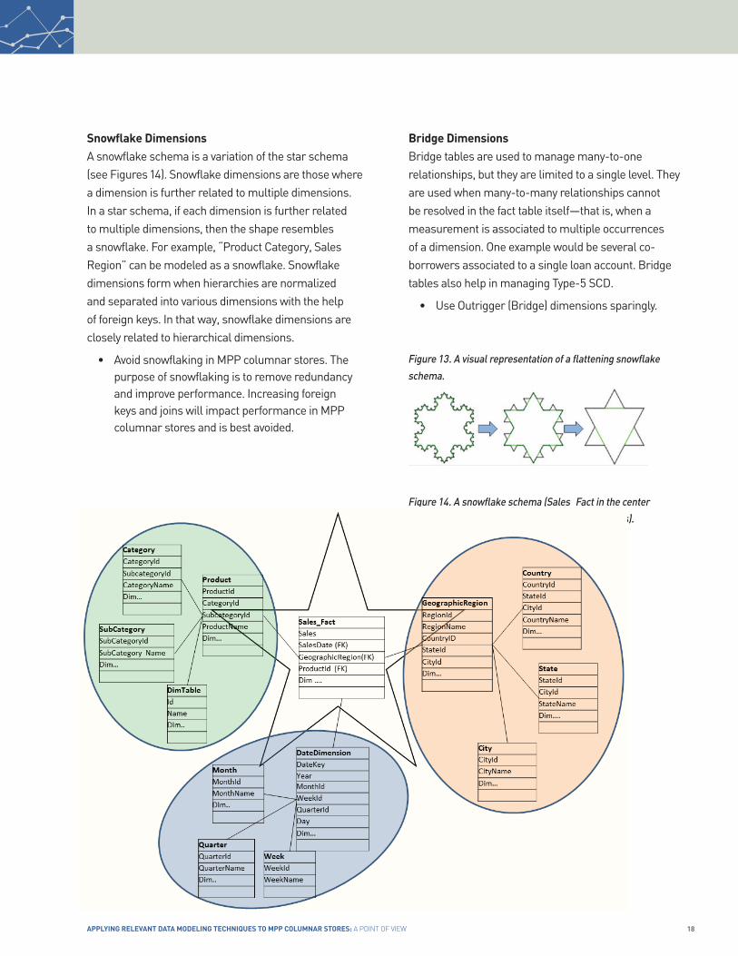
snowflake DimensionsA snowflake schema is a variation of the star schema (see Figures 14). Snowflake dimensions are those where a dimension is further related to multiple dimensions. In a star schema, if each dimension is further related to multiple dimensions, then the shape resembles a snowflake. For example, “Product Category, Sales Region” can be modeled as a snowflake. Snowflake dimensions form when hierarchies are normalized and separated into various dimensions with the help of foreign keys. In that way, snowflake dimensions are closely related to hierarchical dimensions.

• Avoid snowflaking in MPP columnar stores. The purpose of snowflaking is to remove redundancy and improve performance. Increasing foreign keys and joins will impact performance in MPP columnar stores and is best avoided.

bridge Dimensions Bridge tables are used to manage many-to-one relationships, but they are limited to a single level. They are used when many-to-many relationships cannot be resolved in the fact table itself—that is, when a measurement is associated to multiple occurrences of a dimension. One example would be several co-borrowers associated to a single loan account. Bridge tables also help in managing Type-5 SCD.

• Use Outrigger (Bridge) dimensions sparingly.

Figure 13. A visual representation of a flattening snowflake

schema.

Figure 14. A snowflake schema (Sales_Fact in the center

surrounded by dimensions, each having hierarchies).


Figure 15. Shrunken dimensions using conformed attributes.

Figure 16. Junk dimensions being created out of the fact.

Reverse this for MPP columnar stores.

shrunken DimensionsShrunken dimensions are used for aggregating fine-grained data. A shrunken dimension is a subset of another dimension. For example, a month dimension would be a shrunken dimension of the date dimension. The month dimension could be connected to a fact table whose grain is at the monthly level. In a traditional data warehouse, shrunken dimensions should be created using conformed attributes (for example, DateDim › MonthDim (Shrunk)).

• In MPP columnar databases, the need for a shrunken dimension is low because MPPs can have fine granularity.

• Even so, shrunken dimensions cannot be completely ruled out for MPP columnar stores. Use them sparingly after trying out alternative approaches to improve performance.

Mini DimensionsMini dimensions are similar to shrunken dimensions but used in the context of managing a rapidly changing dimension (see Type 4 SCD). Mini dimensions are aggregated out of the original dimensions. Having a range of values, they are specifically created to manage the frequently changing nature of the dimension.

• Avoid mini dimensions in MPP columnar stores (de-normalize them into facts). Newer rows can be inserted and differentiated with the use of latest date and timestamp values.

Conformed DimensionsConformed dimensions remain consistent (that is, they have the same meaning) across all facts in the enterprise data warehouse. Dimensions conform when attributes across tables have the same names and domain contents. For example, the date dimension connected to the sales fact should be the same that is connected to the inventory fact.

• Conformed dimensional attributes are highly recommended for MPP columnar stores, too.

• Conformed dimensions keep the schema simple—eliminating the need to create multiple dimensions having similar columns/data that may confuse end users.

Junk DimensionsJunk dimensions are structures that provide a convenient place to store “junk”—unimportant attributes, such as low cardinality flags and/or text attributes. In MPP columnar stores, junk dimensions are not needed.

• Compress junk dimensions and store them in fact tables to reduce the number of joins.

• This, in turn, avoids creating centipede facts, simplifies ETL and eases maintenance.

DateDimensionDateKey (PK)Date MonthDimensionFullDateDescription MonthKey(PK)MonthName MonthNameMonthNumber MonthNumberMonthFormatYYYY-‐MM MonthFormatYYYY-‐MMYear Year

FiscalMonth QuarterDimensionDayOfWeek QuarterIdQuarter QuarterQuarterName QuarterNameQuarterYearFormatQnYYYY QuarterYearFormatQnYYYY….

JunkDimJunkIdTxn_CodeCoupon_IndicatorPrepayment_Indicator

StoreIdJunkIdTxn_Amount

Txn_Amount

FactTableCustomerIdProductIdTxnId

Prepayment_IndicatorCoupon_IndicatorTxn_CodeStoreIdTxnIdProductIdCustomerIdFactTable

JunkDimJunkIdTxn_CodeCoupon_IndicatorPrepayment_Indicator

StoreIdJunkIdTxn_Amount

Txn_Amount

FactTableCustomerIdProductIdTxnId

Prepayment_IndicatorCoupon_IndicatorTxn_CodeStoreIdTxnIdProductIdCustomerIdFactTable


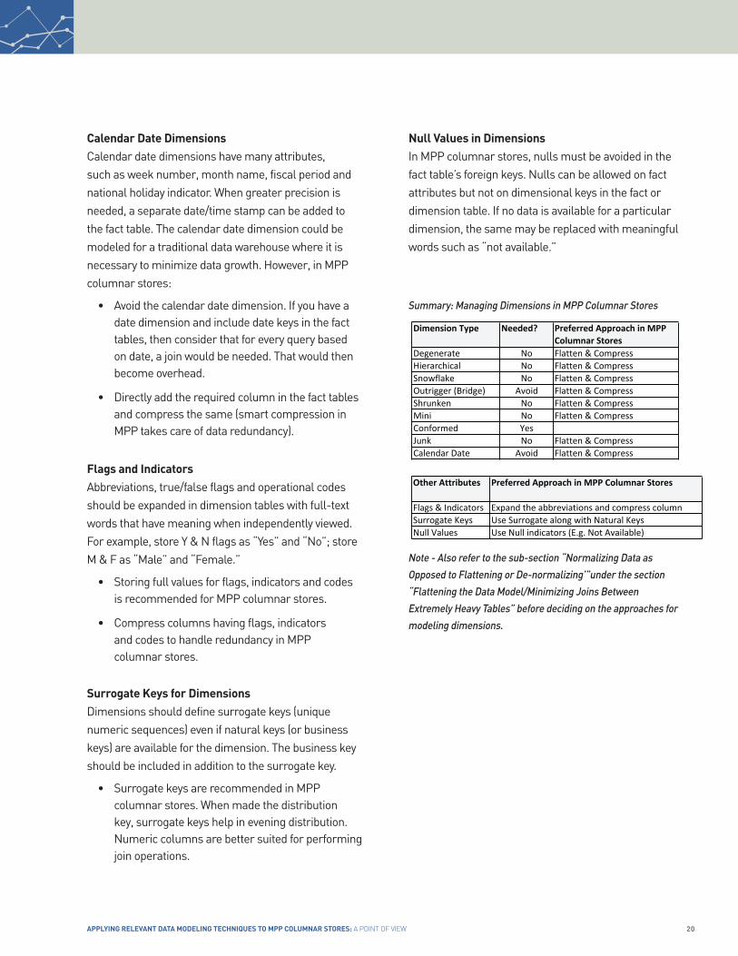
Calendar Date DimensionsCalendar date dimensions have many attributes, such as week number, month name, fiscal period and national holiday indicator. When greater precision is needed, a separate date/time stamp can be added to the fact table. The calendar date dimension could be modeled for a traditional data warehouse where it is necessary to minimize data growth. However, in MPP columnar stores:

• Avoid the calendar date dimension. If you have a date dimension and include date keys in the fact tables, then consider that for every query based on date, a join would be needed. That would then become overhead.

• Directly add the required column in the fact tables and compress the same (smart compression in MPP takes care of data redundancy).

Flags and IndicatorsAbbreviations, true/false flags and operational codes should be expanded in dimension tables with full-text words that have meaning when independently viewed. For example, store Y & N flags as “Yes” and “No”; store M & F as “Male” and “Female.”

• Storing full values for flags, indicators and codes is recommended for MPP columnar stores.

• Compress columns having flags, indicators and codes to handle redundancy in MPP columnar stores.

surrogate Keys for DimensionsDimensions should define surrogate keys (unique numeric sequences) even if natural keys (or business keys) are available for the dimension. The business key should be included in addition to the surrogate key.

• Surrogate keys are recommended in MPP columnar stores. When made the distribution key, surrogate keys help in evening distribution. Numeric columns are better suited for performing join operations.

null Values in DimensionsIn MPP columnar stores, nulls must be avoided in the fact table’s foreign keys. Nulls can be allowed on fact attributes but not on dimensional keys in the fact or dimension table. If no data is available for a particular dimension, the same may be replaced with meaningful words such as “not available.”

Summary: Managing dimensions in MPP Columnar Stores

note - Also refer to the sub-section “normalizing data as

opposed to Flattening or de-normalizing’”under the section

“Flattening the data Model/Minimizing Joins Between

extremely Heavy tables” before deciding on the approaches for

modeling dimensions.

Dimension Type Needed? Preferred Approach in MPP Columnar Stores

Other Attributes

Degenerate No Flatten & Compress Flags & IndicatorsHierarchical No Flatten & Compress Surrogate KeysSnowflake No Flatten & Compress Null ValuesOutrigger (Bridge) Avoid Flatten & CompressShrunken No Flatten & CompressMini No Flatten & CompressConformed YesJunk No Flatten & CompressCalendar Date Avoid Flatten & Compress

Expand the abbreviations and compress columnUse Surrogate along with Natural KeysUse Null indicators (E.g. Not Available)

Preferred Approach in MPP Columnar Stores

Dimension Type Needed? Preferred Approach in MPP Columnar Stores

Other Attributes

Degenerate No Flatten & Compress Flags & IndicatorsHierarchical No Flatten & Compress Surrogate KeysSnowflake No Flatten & Compress Null ValuesOutrigger (Bridge) Avoid Flatten & CompressShrunken No Flatten & CompressMini No Flatten & CompressConformed YesJunk No Flatten & CompressCalendar Date Avoid Flatten & Compress

Expand the abbreviations and compress columnUse Surrogate along with Natural KeysUse Null indicators (E.g. Not Available)

Preferred Approach in MPP Columnar Stores


Figure 17. table showing a summary of techniques for handling slowly changing dimensions.

6. MAnAgIng slowlY ChAngIng DIMensIons

Over time, some dimensions change. Examples include address fields for customers and status of a loan. When the value of a dimension gets updated, there comes the question of how to maintain the earlier value. There are many ways to deal with such slowly changing dimensions.

The table (Figure 17) below summarizes techniques for handling slowly changing dimensions in traditional data warehouse systems.

Many of these approaches for managing slowly changing dimensions have been pioneered by Ralph Kimball. While Kimball has defined a few more techniques (types 5, 6 and 7), they are a combination of the above and are rarely used.

Here are some things to consider when choosing the right method for addressing slowly changing dimensions in MPP columnar stores:

• Dealing with slowly changing dimensions is driven first by business needs and then by underlying data warehousing technology.

• Try to keep things simple. In many cases, type-3 (“Add column”) can be suitable for MPP columnar stores.

• Types 4, 5 and 7 are used for managing the grain of the fact to acceptable levels, managing volatile dimensional changes and for analyzing demographics. If none of these are needed, type 2 or 3 may be used.

• Perform tests and try different types before finalizing an approach. Also consider efforts involved at the ETL layer for managing data before finalizing the approach.

Refer to the Appendix for a quick primer on slowly changing dimensions.

SCD Type 0

1

2

3

4

5

Action taken on dimension tableFacts will continue to be associated with the original value and not the newer value

History data is lost and facts are mapped only to current dimensional value.

An indicator column identifies the current value of the dimension. All other values are older values.

Add new column to retain current and prior dimension values

Associated Impact

Facts can be mapped to both old and current values. The newer column can be named indicating that it has the current value.Dimensional data is present in both original table and the newly created mini table. Mini table stores historical data while current data exits in the base table.

With the mini dimension key being over-‐written in the base table, the facts will only be associated with the latest rapidly changing values

Add mini-‐dimension table to manage rapidly changing dimensions. Add type 4 mini-‐dimension to store current changes. Maintain a foreign key on the base dimension table pointing to this mini table and over-‐write this

Make no change.

Overwrite older value with newer value

Add a new row with the latest value retaining both old and new values.


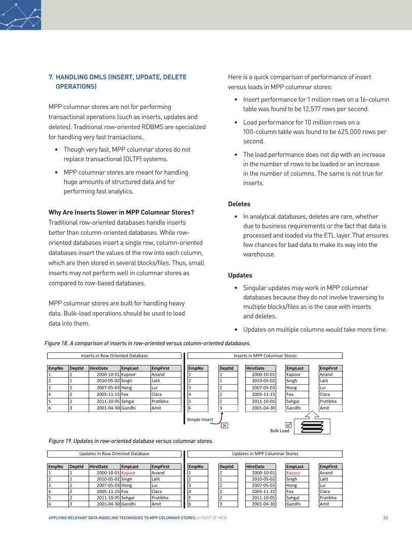
7. hAnDlIng DMls (InseRt, UPDAte, Delete oPeRAtIons)

MPP columnar stores are not for performing transactional operations (such as inserts, updates and deletes). Traditional row-oriented RDBMS are specialized for handling very fast transactions.

• Though very fast, MPP columnar stores do not replace transactional (OLTP) systems.

• MPP columnar stores are meant for handling huge amounts of structured data and for performing fast analytics.

why Are Inserts slower in MPP Columnar stores?Traditional row-oriented databases handle inserts better than column-oriented databases. While row-oriented databases insert a single row, column-oriented databases insert the values of the row into each column, which are then stored in several blocks/files. Thus, small inserts may not perform well in columnar stores as compared to row-based databases.

MPP columnar stores are built for handling heavy data. Bulk-load operations should be used to load data into them.

Here is a quick comparison of performance of insert versus loads in MPP columnar stores:

• Insert performance for 1 million rows on a 16-column table was found to be 12,577 rows per second.

• Load performance for 10 million rows on a 100-column table was found to be 625,000 rows per second.

• The load performance does not dip with an increase in the number of rows to be loaded or an increase in the number of columns. The same is not true for inserts.

Deletes

• In analytical databases, deletes are rare, whether due to business requirements or the fact that data is processed and loaded via the ETL layer. That ensures few chances for bad data to make its way into the warehouse.

Updates

• Singular updates may work in MPP columnar databases because they do not involve traversing to multiple blocks/files as is the case with inserts and deletes.

• Updates on multiple columns would take more time.

Figure 18. A comparison of inserts in row-oriented versus column-oriented databases.

Figure 19. updates in row-oriented database versus columnar stores.

EmpNo DeptId HireDate EmpLast EmpFirst EmpNo DeptId HireDate EmpLast EmpFirst1 1 2000-‐10-‐01 Kapoor Anand 1 1 2000-‐10-‐01 Kapoor Anand2 1 2010-‐05-‐02 Singh Lalit 2 1 2010-‐05-‐02 Singh Lalit3 2 2007-‐05-‐03 Hong Lui 3 2 2007-‐05-‐03 Hong Lui4 2 2005-‐11-‐15 Fox Clara 4 2 2005-‐11-‐15 Fox Clara5 2 2011-‐10-‐05 Sehgal Pratibha 5 2 2011-‐10-‐05 Sehgal Pratibha6 3 2001-‐04-‐30 Gandhi Amit 6 3 2001-‐04-‐30 Gandhi Amit

Updates in Row Oriented Database Updates in MPP Columnar Stores

EmpNo DeptId HireDate EmpLast EmpFirst EmpNo DeptId HireDate EmpLast EmpFirst1 1 2000-‐10-‐01 Kapoor Anand 1 1 2000-‐10-‐01 Kapoor Anand2 1 2010-‐05-‐02 Singh Lalit 2 1 2010-‐05-‐02 Singh Lalit3 2 2007-‐05-‐03 Hong Lui 3 2 2007-‐05-‐03 Hong Lui4 2 2005-‐11-‐15 Fox Clara 4 2 2005-‐11-‐15 Fox Clara5 2 2011-‐10-‐05 Sehgal Pratibha 5 2 2011-‐10-‐05 Sehgal Pratibha6 3 2001-‐04-‐30 Gandhi Amit 6 3 2001-‐04-‐30 Gandhi Amit

Inserts in Row Oriented Database Inserts in MPP Columnar Stores

x þ Bulk Load

Simple Insert


best Practices for DMls in MPP Columnar Databases

Inserts 1. Use bulk loading in MPP columnar databases to

populate the table. Avoid normal insert statements. (This applies for initial as well as periodic data loads.)

2. For inserts that increase the database size by 30 to 40 percent, evaluate truncating/dropping the table and using bulk load options.

3. Where possible, try to use: a. Create Table As Select (CTAS) to quickly load data or b. Use INSERT INTO TABLE (SELECT * FROM

<Table>).

Deletes1. For significant deletes (more than 40 percent of table

size), bulk load data into a new table. Drop the older table and rename the new table back to the older table.

2. Consolidate deletes (within a table and across multiple tables) and perform them together—preferably during off-peak hours or over the weekend.

3. Perform deletes when absolutely needed. If there are very few deletes to be done on a multi-million-row table, consider handling them in the BI layer instead of deleting in the table. Allow for consolidation of deletes as explained in step 2.

4. Many MPP columnar stores do not enforce referential constraints. Therefore, ensure that the values get deleted in all related tables manually.

UpdatesConsider two important aspects for updates in MPP:1. For dimensional tables, follow rules for managing

slowly changing dimensions.2. When updating the DistKey column, watch out for a

resulting data skew.

Following are the best practices for making updates in MPP columnar databases:1. Follow the rules of SCD when updating dimensional

data.2. Many MPP columnar stores do not enforce referential

constraints. Ensure that the values get updated in all related tables.

3. For significant updates (more than 40 percent of table size), consider truncating or dropping the table and loading the values afresh.

4. Consolidate all the updates within the table and across all tables and perform them together during off-peak hours or over the weekend.

5. After updating a significant portion of a multi-million-row table, ensure that the data is redistributed and measures are taken to update statistics on the table. This will remove any skewing that may have been caused by the update.


The Big Data world is complex and is still evolving. While traditional technologies, such as ETL, data warehouse and BI tools, still work in the structured data realm, there is a whole new stack of technologies that have come up to acquire, process and integrate unstructured data sources. Adapters and connectors help to bridge both worlds—especially between the data warehouse, MPP columnar store and the Hadoop-Big Data platform world.

MPP columnar databases have started figuring in the overall Big Data landscape but remain focused on the structured data layer. That is because pure data warehouse systems and appliances cannot deal effectively or scale when it comes to managing voluminous data (that is, more than a few terabytes), and data volumes continue to grow.

Here are a few terms pertaining to the Big Data platform:

• hadoop is a framework for processing, storing and analyzing large volumes of unstructured data (Big Data) applications on a large commodity cluster. Key components include Map Reduce and HDFS.

• Map Reduce is a computational technique that divides applications into many small fragments of work. Divided in two, the “Map” function divides a query into multiple parts and processes data at the node level. The “Reduce” function aggregates the results of the “Map” function to determine the “answer” to the query.

• hDFs is the storage layer of Hadoop. It is distributed and scalable, with a Java-based file system adept in storing large volumes of unstructured data.

wheRe/how Do MPP ColUMnAR stoRes FIt In the bIg DAtA ARChIteCtURe?

Figure 20. Big data architectural components.


• hive, originally developed by Facebook, is a Hadoop-based framework for doing data warehousing-like jobs. It allows users to query in SQL-like language (HiveQL). Queries are then converted to Map Reduce, allowing programmers with no experience in Map Reduce to use the underlying (Big Data) store for analytics and integrate with BI and visualization tools.

• Pig, or Pig Latin, is a Hadoop-based language developed by Yahoo. Easy to work with, it is adept in very deep, very long data pipelines.

• hbase is a non-relational database that allows low-latency, quick lookups in Hadoop. It adds transactional capabilities (inserts, updates and deletes) to Hadoop.

• Cassandra is an open source distributed database management system designed to handle large amounts of data across many commodity servers. As such, it provides high availability with no single point of failure. Cassandra offers robust support for clusters spanning multiple data centers, with asynchronous master-less replication allowing low latency operations for all clients.

• Flume is a distributed, reliable and available service for efficiently collecting, aggregating and moving large amounts of log data. It has a simple and flexible architecture based on streaming data flows.

• oozie is a workflow processing system that lets users define a series of jobs written in multiple languages—such as Map Reduce, Pig and Hive—and then intelligently link them to one another. Oozie allows users to specify that a particular query is only to be initiated after specified previous jobs on which it relies for data are completed.

• Mahout is a data mining library. It takes the most popular data mining algorithms for performing clustering, regression testing and statistical modeling and implements them using the Map Reduce model.

• sqoop is a connectivity tool for moving data from non-Hadoop data stores, such as relational databases and data warehouses, into Hadoop. It allows users to specify the target location inside of Hadoop and instruct Sqoop to move data from Oracle, Teradata or other relational databases to the target.

• hcatalog is a centralized metadata management and sharing service for Apache Hadoop. It allows for a unified view of all data in Hadoop clusters. It also allows diverse tools, including Pig and Hive, to process any data elements without needing to know where in the cluster the data is physically stored.

wheRe/how Do MPP ColUMnAR stoRes FIt In the bIg DAtA ARChIteCtURe?


MPP columnar databases bring a compelling set of advantages and are quickly becoming an integral part of all Big Data solution architectures. MPP columnar databases process and help analyze enormous volumes of structured data. They also aid in analyzing structured data out of the unstructured “Big Data” sources.

Traditional row-based data warehouses have struggled to deliver the needed scalability, ROI, time to market, speed, flexibility and responsiveness. MPP columnar databases deliver against these needs.

Given that MPP columnar databases are designed to support analytics from the core, most dimensional modeling approaches work for them. Even so, rules can be modified to make them simpler and more relevant thanks to the underlying architecture and inherent advantages of MPP columnar databases.

This point of view has brought together the various approaches, techniques and best practices for data modeling using MPP columnar stores. Key takeaways include:

• The value of a simpler approach versus designing intricate, normalized schema

• Denormalizing and flattening tables where possible

• Recognizing data distribution and data co-location as key factors

• The need for consistent use of compression, which helps efficiently manage data volumes and redundancy

• The need to consider ETL processes in conjunction with overall schema design in MPP columnar stores

• The value of testing various approaches (distribution, insert versus bulk load, flattening versus dimensional) before finalizing one

Finally, this point of view asserts that no single approach is perfect. Everything comes with tradeoffs—necessitating a hybrid approach.

Do try these approaches and techniques when dealing with MPP columnar products, and kindly share your experiences and feedback with me at [email protected].

ConClUsIon

mailto:susrinivasan%40sapient.com?subject=MMP%20columnar%20products


I would like to thank and acknowledge the Sapient Global Markets Technology Capability team and the DSST team in reviewing this document and providing valuable suggestions and feedback.

The Internet has been a huge resource and reference by way of articles, white papers, e-books and e-publications. Some of the important books and white papers referenced include:

The Data Warehouse Toolkit, 3rd Edition – by Ralph Kimball & Margy Ross

Data Warehousing in the Age of Big Data – by Krish Krishnan

Building the Data Warehouse, 4th Edition – by WH Inmon

Amazon RedShift & ParAccel Analytical Database documentation

Articles on Big Data & Hadoop from wikibon.org BI & DW Articles from kimballgroup.com

ConClUsIon ReFeRenCes & ACKnowleDgeMents


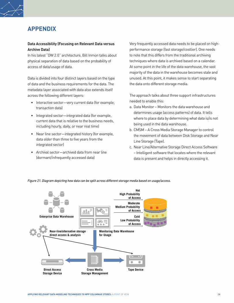
Data Accessibility (Focusing on Relevant Data versus Archive Data)In his latest “DW 2.0” architecture, Bill Inmon talks about physical separation of data based on the probability of access of data/usage of data.

Data is divided into four distinct layers based on the type of data and the business requirements for the data. The metadata layer associated with data also extends itself across the following different layers:

• Interactive sector—very current data (for example, transaction data)

• Integrated sector—integrated data (for example, current data that is relative to the business needs, including hourly, daily, or near real time)

• Near line sector—integrated history (for example, data older than three to five years from the integrated sector)

• Archival sector—archived data from near line (dormant/infrequently accessed data)

Very frequently accessed data needs to be placed on high-performance storage (fast storage/costlier). One needs to note that this differs from the traditional archiving techniques where data is archived based on a calendar. At some point in the life of the data warehouse, the vast majority of the data in the warehouse becomes stale and unused. At this point, it makes sense to start separating the data onto different storage media.

The approach talks about three support infrastructures needed to enable this:a. Data Monitor – Monitors the data warehouse and

determines usage (access patterns) of data. It tells where to place data by determining what data is/is not being used in the data warehouse.

b. CMSM – A Cross Media Storage Manager to control the movement of data between Disk Storage and Near Line Storage (Tape).

c. Near Line/Alternative Storage Direct Access Software – Intelligent software that locates where the relevant data is present and helps in directly accessing it.

APPenDIX

Figure 21. diagram depicting how data can be split across different storage media based on usage/access.

Enterprise Data Warehouse

Near-line/alternative storage direct access & analysis

Monitoring Data Warehousefor Usage

Hot High Probability

of Access

Moderate Medium Probability

of Access

Cold Low Probability

of Access

Direct AccessStorage Device

Cross MediaStorage Management

Tape Device


Pros1. This brings in a radically new approach to managing

data volumes. Storage costs associated with fast storage are optimized, thereby boosting the performance of the data warehouse.

2. Data is online but is kept in fat volume stores, which can store heavy data and cost less as compared to fast storage.

3. With overflow storage, the designer is free to create as low a level of granularity as desired.

Cons1. In MPP columnar stores, data is distributed among the

compute nodes, rendering this approach irrelevant.2. Ad-hoc queries, which are rare, may lead to the data

monitor triggering dormant/stale data to be loaded to direct access storage device.

3. The access/usage patterns of data may vary significantly, thereby rendering useless all the effort of splitting data.

quick Primer on slowly Changing Dimensions(the examples and other details in this section have been referenced from the data Warehouse toolkit, 3rd edition by Ralph Kimball & Margy Ross.)

type 0 (Retain original)Here, the original facts value of the dimension is kept unchanged. For any attribute named “Original” (such as the customer’s original credit score, audit columns such as created by and created date, or many of the date dimensions) are always grouped by the original value. This has no impact in MPP columnar databases.

type 1 (overwrite)Here, you overwrite the old attribute value in the dimension row, replacing it with the current value. The attribute always reflects the most recent assignment. The fact table is untouched.

Pros

• Easy to implement

• Does not increase storage cost as the original value is overwritten

Cons

• The problem with a type 1 response is the loss of all history of attribute changes

• A type 1 response is appropriate if the attribute change is an insignificant correction

• It also may be appropriate if there is no value in keeping the old description

• BI/Reporting results may vary following the change

• Any preexisting aggregations based on the department value need to be rebuilt

• Even OLAP cubes need to be reprocessed if the updated dimension was part of the cube

APPenDIX

Figure 22. Managing slowly changing dimensions via the type 1 method.

ProductId NaturalKey ProductName DollarUnitprice ProductDescription ProductDepartment121 PRD-‐123-‐2 ProdABC 160 Prod ABC description Education Sw update/over-‐write

Project Management Sw

ProductId NaturalKey ProductName DollarUnitprice ProductDescription ProductDepartment121 PRD-‐123-‐2 ProdABC 160 Prod ABC description Project Management Sw

Type-‐1 SCD OverWrite


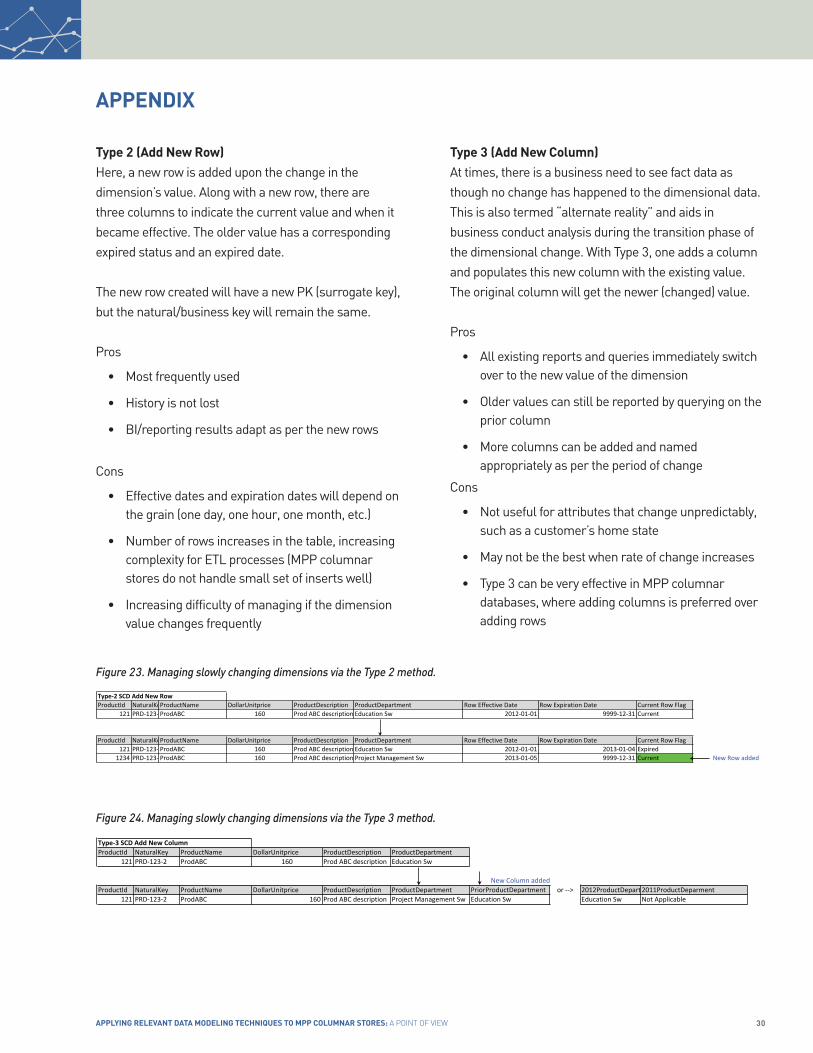
type 2 (Add new Row)Here, a new row is added upon the change in the dimension’s value. Along with a new row, there are three columns to indicate the current value and when it became effective. The older value has a corresponding expired status and an expired date.

The new row created will have a new PK (surrogate key), but the natural/business key will remain the same.

Pros

• Most frequently used

• History is not lost

• BI/reporting results adapt as per the new rows

Cons

• Effective dates and expiration dates will depend on the grain (one day, one hour, one month, etc.)

• Number of rows increases in the table, increasing complexity for ETL processes (MPP columnar stores do not handle small set of inserts well)

• Increasing difficulty of managing if the dimension value changes frequently

type 3 (Add new Column)At times, there is a business need to see fact data as though no change has happened to the dimensional data.This is also termed “alternate reality” and aids in business conduct analysis during the transition phase of the dimensional change. With Type 3, one adds a column and populates this new column with the existing value. The original column will get the newer (changed) value.

Pros

• All existing reports and queries immediately switch over to the new value of the dimension

• Older values can still be reported by querying on the prior column

• More columns can be added and named appropriately as per the period of change

Cons

• Not useful for attributes that change unpredictably, such as a customer’s home state

• May not be the best when rate of change increases

• Type 3 can be very effective in MPP columnar databases, where adding columns is preferred over adding rows

APPenDIX



ProductId NaturalKeyProductName DollarUnitprice ProductDescription ProductDepartment Row Effective Date Row Expiration Date Current Row Flag121 PRD-‐123-‐2ProdABC 160 Prod ABC description Education Sw 2012-‐01-‐01 9999-‐12-‐31 Current

ProductId NaturalKeyProductName DollarUnitprice ProductDescription ProductDepartment Row Effective Date Row Expiration Date Current Row Flag121 PRD-‐123-‐2ProdABC 160 Prod ABC description Education Sw 2012-‐01-‐01 2013-‐01-‐04 Expired1234 PRD-‐123-‐2ProdABC 160 Prod ABC description Project Management Sw 2013-‐01-‐05 9999-‐12-‐31 Current New Row added

Type-‐2 SCD Add New Row

ProductId NaturalKey ProductName DollarUnitprice ProductDescription ProductDepartment121 PRD-‐123-‐2 ProdABC 160 Prod ABC description Education Sw

New Column addedProductId NaturalKey ProductName DollarUnitprice ProductDescription ProductDepartment PriorProductDepartment or -‐-‐> 2012ProductDepartment2011ProductDeparment

121 PRD-‐123-‐2 ProdABC 160 Prod ABC description Project Management Sw Education Sw Education Sw Not Applicable

Type-‐3 SCD Add New Column


type 4 (Add new table)Here, a new but smaller table is created to store the frequent change in the value of the dimension. Customer demographics that change frequently—such as age, purchase frequency and income level—can be stored in such a table. There would be one row in the mini dimension for each unique combination of age, purchase frequency score, and income level encountered in the data, rather than one row per customer.

When creating the mini dimension, continuously variable attributes are converted to banded ranges. This is used to keep the number of rows to a much smaller level. The mini dimension key participates as a foreign key in the fact table; thus, the fact table captures the demographic profile changes.

Pros

• Demographic values can be captured in the fact

• Helps in keeping the fact table size to a manageable level

Cons

• Frequent use of mini dimensions for a specific fact can help form centipede facts, which are best avoided

Type 5, 6 and 7 have been kept out of scope of this document and may be referenced on Kimball’s data warehousing website:http://www.kimballgroup.com/2013/02/05/design-tip-152-slowly-changing-dimension-types-0-4-5-6-7/

APPenDIX


Customer Dim FactTable Demographics Dim DemographicsKey AgeBand PurchaseFrequency IncomeBandCustKey (PK) CustKey(FK) DemographicsKey(PK) 1 21-‐25 Low <$40,000CustId (NK) DateKey(FK) AgeBand 2 21-‐25 Medium <$40,000CustName DemographicKey(FK) PurchaseFrequencyScore 3 21-‐25 High <$40,000CustAddress Facts. . . . Income Band 4 21-‐25 Low $40,000 -‐ 50,000CustCity 5 21-‐25 Medium $40,000 -‐ 50,000CustState 6 26-‐30 High $40,000 -‐ 50,000CustZipCode … … … …CustDOB 7 26-‐30 Low <$40,000

8 26-‐30 Medium <$40,000

Type-‐4 SCD Mini Dimension

Customer Dim FactTable Demographics Dim DemographicsKey AgeBand PurchaseFrequency IncomeBandCustKey (PK) CustKey(FK) DemographicsKey(PK) 1 21-‐25 Low <$40,000CustId (NK) DateKey(FK) AgeBand 2 21-‐25 Medium <$40,000CustName DemographicKey(FK) PurchaseFrequencyScore 3 21-‐25 High <$40,000CustAddress Facts. . . . Income Band 4 21-‐25 Low $40,000 -‐ 50,000CustCity 5 21-‐25 Medium $40,000 -‐ 50,000CustState 6 26-‐30 High $40,000 -‐ 50,000CustZipCode … … … …CustDOB 7 26-‐30 Low <$40,000

8 26-‐30 Medium <$40,000

Type-‐4 SCD Mini Dimension

http://www.kimballgroup.com/2013/02/05/design-tip-152-slowly-changing-dimension-types-0-4-5-6-7/

http://www.kimballgroup.com/2013/02/05/design-tip-152-slowly-changing-dimension-types-0-4-5-6-7/


quick Primer on Facts and Fact types(the examples and other details in this section have been referenced from the data Warehouse toolkit, 3rd edition by Ralph Kimball & Margy Ross.)

In the world of data warehousing, facts are measurements that result from a business process event and are almost always numeric. In a sales transaction, for instance, the numeric measurements may include the quantity of a product sold and its extended price.

There are various types of facts, which are described briefly.

Fully Additive Facts These are measures that can be summed across all the dimensions of the fact table. Examples include sales quantity, discount provided, cost dollar amount and gross profit, which can be calculated across stores, dates or products. As such, they are fully additive.

semi Additive Facts These are not additive across all dimensions—especially time. For example, inventory levels are non-additive across dates as they represent snapshots at a particular time. Similarly, financial account balances are also semi-additive.

non Additive Facts Some measures, such as ratios, are not additive. For non-additive facts, where possible, store the fully additive components of the non-additive measure and sum these components into the final answer set before calculating the final non-additive fact.

In an inventory schema, one may also store QuantityBeginningBalance, InventoryChange or Delta and QuantityEndingBalance. The balance amounts are semi-additive but the deltas are fully additive facts. For example, all measures that record a static level (inventory levels, financial account balances and measures of intensity, such as room temperatures) are inherently non-additive across the date dimension and possibly other dimensions. In these cases, the measure can be aggregated across dates by averaging over the number of time periods.

APPenDIX

Figure 26. A visual representation of various fact types.

DegenerateDimensions

HierarchicalDimensions

JunkDimensions

Slowly Changing

Dimensions

DimensionTypes

Mini/ShrunkenDimensions

SnowFlakeDimensions

OutriggerDimensions

ConformedDimensions

FactTypes

Additivefull, semi, non

Facts

TransactionFacts

ConsolidatedFacts

AggregateFacts

FactlessFact

Accum,Snapshot

Facts

PeriodicSnapshot

Facts

ConformedFacts


transaction Facts This fact type stores data corresponding to a measurement event at a point in time. They are the most common fact type. These fact tables always contain a foreign key for each associated dimension, thereby enabling the maximum slicing and dicing of transaction data. OrderTransaction is an example.

Conformed Facts These are measurements (columns) that appear in different fact tables. If the separate fact definitions are consistent, the conformed facts should be identically named. However, if they are incompatible, they should be differently named. For instance, revenue, profit, standard prices and costs, measures of quality and customer satisfaction, and other key performance indicators (KPIs) are facts that must conform.

Periodic snapshot Facts The periodic snapshot fact table summarizes many measurement events occurring over a standard period, such as a day, week or month. The grain is the period, not the individual transaction. An example is inventory quantity in hand.

APPenDIX

Figure 27. An example of a transaction fact.

Figure 28. An example of a periodic snapshot fact.

DateDimDateKey (PK)

CustomerDimSalesRepDim CustomerKey (PK)SalesRepKey (PK)

ProductDimProductKey (PK)

OrderTransaction_FactOrderDateKey (FK)CustomerKey (FK)ProductKey (FK)SalesRepKey (FK)OrderNumberOrderLineNumberOrderQuantityFacts…

DateDimDateKey (PK)

StoreDim ProductDimStoreKey (PK) ProductKey (PK)Facts…

DateKey (FK)Store Inventory Snapshot Fact

StoreKey (FK)ProductKey (FK)

QuantityOnHand


Accumulating snapshot Facts This type of fact table describes what has happened over a period of time—including pipeline or workflow processes, such as order fulfillment or claim processing. Therefore, this fact table summarizes the measurement events occurring at predictable steps between the beginning and end of a process. As progress occurs, the accumulating fact table row is revisited and updated. This consistent updating of accumulating snapshot fact rows is unique among the three types of fact tables. Order tracking is an example of an accumulating snapshot.

Consolidated Facts Provided that they can be expressed in the same grain, these are a combination of facts from multiple sources. For example, sales forecast and sales actuals can be combined in a single table for simpler comparisons and analysis.

Aggregate Fact (olAP Cubes) Aggregate fact tables are simple numeric rollups of atomic fact table data built solely to accelerate query performance. An aggregate fact is often built from a fine-grained fact as seen in the example below. The grain of the fine grained table (left) is a day (date of order) while the grain for the aggregated table (right) is that of sum of unit sales for a month.

Figure 29. An example of an accumulating snapshot fact.

OrderTrackingOrderNumberOrderDate (FK)ShipDate (FK)DeliveryDate(FK)PaymentDate (FK)QAPassDate (FK)ReturnDate (FK)PortScanDate (FK)PortId (FK)StoreID (FK)CustomerID (FK)OrderStatus (FK)QuantityOrderedExtendedListPriceDiscountsExtendedNetPrice

Date as per progression of the order

Facts pertaining to order (will remain same)

Airport or City border item check

Current order status (gets updated at regular intervals)


Factless FactThese are facts that have only associated dimensions and do not have numeric measures. For example, an event such as a student attending a class does not have a numeric fact, but the fact row has foreign keys for date, student, teacher and class. Factless facts can also be used to analyze what did not happen. Absenteeism is an example.

Figure 30. An example of an aggregate fact being created out of fine grained fact table.

Figure 31. example of a factless fact.

CustID Item No Order Date Unit Sales Profit CustID Item No Order date Unit Sales Profit191 143 4/5/98 1 1.52 191 150 Jan-‐98 11 11.52191 150 4/5/98 3 3.9 191 150 Feb-‐98 3 3.9191 8 10/6/98 1 2.48 191 150 Mar-‐98 2 2.48191 77 10/6/98 1 1.37 191 150 Apr-‐98 1 1.37191 92 10/6/98 1 1.33 191 150 May-‐98 1 1.33191 95 10/6/98 1 2.87 191 150 Jun-‐98 2 2.87191 18 28/07/1998 1 2.3191 37 28/07/1998 1 1.03191 61 28/07/1998 1 2.01191 83 28/07/1998 1 2.37191 120 28/07/1998 1 2.24191 8 13/08/1998 1 2.48191 58 13/08/1998 1 2.79191 100 16/12/1998 1 2.18191 122 16/12/1998 1 2.47191 83 12/5/99 1 2.37191 148 12/5/99 1 2.17191 37 29/11/1999 1 1.03191 116 29/11/1999 1 2.03211 46 7/4/98 1 2.24211 110 7/4/98 1 2.84211 49 6/5/98 1 2.2211 60 6/5/98 1 1.91211 26 22/05/1998 1 1.69

CustID Item No Order Date Unit Sales Profit CustID Item No Order date Unit Sales Profit191 143 4/5/98 1 1.52 191 150 Jan-‐98 11 11.52191 150 4/5/98 3 3.9 191 150 Feb-‐98 3 3.9191 8 10/6/98 1 2.48 191 150 Mar-‐98 2 2.48191 77 10/6/98 1 1.37 191 150 Apr-‐98 1 1.37191 92 10/6/98 1 1.33 191 150 May-‐98 1 1.33191 95 10/6/98 1 2.87 191 150 Jun-‐98 2 2.87191 18 28/07/1998 1 2.3191 37 28/07/1998 1 1.03191 61 28/07/1998 1 2.01191 83 28/07/1998 1 2.37191 120 28/07/1998 1 2.24191 8 13/08/1998 1 2.48191 58 13/08/1998 1 2.79191 100 16/12/1998 1 2.18191 122 16/12/1998 1 2.47191 83 12/5/99 1 2.37191 148 12/5/99 1 2.17191 37 29/11/1999 1 1.03191 116 29/11/1999 1 2.03211 46 7/4/98 1 2.24211 110 7/4/98 1 2.84211 49 6/5/98 1 2.2211 60 6/5/98 1 1.91211 26 22/05/1998 1 1.69

Fact_AttendanceStudent_id (FK)Teacher_Id (FK)DateKey (FK)ClassId (FK)

Student Dim

Teacher Dim

Date Dim


globAl oFFICesGenevaSuccursale Genèvec/o Florence Thiébaud, avocaterue du Cendrier 151201 GenevaSwitzerlandTel: +41 (0) 58 206 06 00

HoustonHeritage Plaza1111 Bagby Street Suite 1950Houston, TX 77002Tel: +1 (713) 493 6880

LondonEden House8 Spital SquareLondon, E1 6DUUnited KingdomTel: + 44 (0) 207 786 4500

Los Angeles1601 Cloverfield Blvd.Suite 400 SouthSanta Monica, CA 90404Tel: +1 (310) 264 6900

MilanSapient Italy S.r.lViale Bianca Maria 2320122 MilanItalyTel: +39-02-36269529

MumbaiSapient Consulting Pvt. LtdR-Tech Park, Goregaon(E)13th Floor, Building 2,Off Western Express HighwayMumbai, Maharashtra - 400063IndiaTel: +91-22-44764567

Munich Arnulfstrasse 6080335 MünchenGermanyTel: +49 (0) 89 552 987 0

Noida(NCR of Delhi)“Oxygen”, Tower C,Ground - 3rd floorPlot No. 7,Sector 144 ExpresswayNoida 201304Uttar PradeshIndiaTel: +91 (120) 479 5000

New York40 Fulton Street22nd FloorNew York, NY 10038Tel: +1 (212) 206 1005

Singapore158 Cecil Street, #03-01Singapore 069545Tel: +65 6671 4933

Toronto129 Spadina Avenue Suite 500Toronto, Ontario M5V 2L3CanadaTel: +1 (416) 645 1500

Washington DC1515 North Courthouse Road4th FloorArlington, VA 22201-2909Tel: +1 (703) 908 2400

ZürichSeefeldstrasse 358008 ZürichSwitzerlandTel: +41 (58) 206 06 00

headquartersBoston131 Dartmouth Street3rd FloorBoston, MA 02116Tel: +1 (617) 621 0200

BangaloreSalarpuria GR Tech Park6th Floor, “VAYU” Block#137, Bengaluru 560066KarnatakaIndiaTel: +91 (080) 410 47 000

Calgary888 3rd Street SWSuite 1000Calgary, Alberta T2P 5C5CanadaTel: +1 (403) 444 5574

Chicago30 West Monroe,12th FloorChicago, IL 60603Tel: +1 (312) 458 1800

DelhiUnitech InfospaceGround Floor, Tower ABuilding 2, Sector 21Old Delhi - Gurgaon RoadDundahera, Gurgaon 122016HaryanaIndiaTel: +91 (124) 499 6000

DüsseldorfSpeditionstrasse 2140221 DüsseldorfGermanyTel: +49 (0) 211 540 34 0

FrankfurtSkyper Villa Taunusanlage 1 60329 Frankfurt Germany Tel: +49 (0)69 505060594

http://www.sapient.com/en-us/global-markets.html

data modeling · disadvantages of mpp columnar stores 8 ... teradata aster data, paraccel analytic...

Documents