data profiling - hasso-plattner-institut · data profiling a sigmod 2017 tutorial ziawasch abedjan...
TRANSCRIPT

Data Profilinga SIGMOD 2017 Tutorial
Ziawasch Abedjan (TU Berlin)Lukasz Golab (University of Waterloo)
Felix Naumann (HPI)

If we just have a bunch of data sets in a repository, it is unlikely anyone will ever be able to find, let alone reuse, any of this data. With adequate metadata, there is some hope,
but even so, challenges will remain..
Data Profiling | SIGMOD 2017 | Chicago Chart 2
[D. Agrawal, P. Bernstein, E. Bertino, S. Davidson, U. Dayal, M. Franklin, J. Gehrke, L. Haas, A. Halevy, J. Han, H. V. Jagadish, A. Labrinidis, S. Madden, Y. Papakonstantinou, J. M. Patel, R. Ramakrishnan, K. Ross, C. Shahabi, D. Suciu, S. Vaithyanathan, and J. Widom. Challenges and opportunities with Big Data. Technical report, Computing Community Consortium, http://cra.org/ccc/docs/ init/bigdatawhitepaper.pdf, 2012.]

Data Profiling | SIGMOD 2017 | Chicago 3

Tutorial Overview• Motivation
• Task classification• Use cases
• Tools• Research and industry• Shortcomings
• Single and Multiple Column Analysis• Cardinalities and datatypes• Co-occurrences and summaries
• Dependencies• UCCs, FDs, ODs, INDs• and their discovery algorithms
• Outlook• Functionality• Semantics
Data Profiling | SIGMOD 2017 | Chicago 4

Data Profiling | SIGMOD 2017 | Chicago 5

Profiling in Spreadsheets
Data Profiling | SIGMOD 2017 | Chicago 6

Data Profiling | SIGMOD 2017 | Chicago 7

Data Profiling | SIGMOD 2017 | Chicago 8

Data Profiling | SIGMOD 2017 | Chicago 9

Many interesting questions remain• What are possible keys and foreign keys?
• Phone• firstname, lastname, street
• Are there any functional dependencies?• zip -> city• race -> voting behavior
• Which columns correlate?• Date-of-Birth and first name• State and last name
• What are frequent patterns in a column?• ddddd• dd aaaa St
Data Profiling | SIGMOD 2017 | Chicago 10

Classification of Traditional Profiling Tasks
Data Profiling | SIGMOD 2017 | Chicago 12
Data
pro
filin
g
Single column
Cardinalities
Patterns and data types
Value distributions
Multiple columns
Uniqueness
Key discovery
Conditional
Partial
Inclusion dependencies
Foreign key discovery
Conditional
Partial
Functional dependencies
Conditional
Partial

Data Profiling vs. Data Mining
• Data profiling gathers technical metadata to support data management• Data mining and data analytics discovers non-obvious results to support
business management
• Data profiling results: information about columns and column sets• Data mining results: information about rows or row sets
• clustering, summarization, association rules, …
• Rahm and Do on data cleaning• Profiling: Individual attributes• Mining: Multiple attributes
[Rahm and Do, Data Cleaning: Problems and Current Approaches, IEEE DE Bulletin, 2000]
Data Profiling | SIGMOD 2017 | Chicago 13

Challenges of (Big) Data Profiling
• Large search space• Number of rows AND number of columns (and column combinations)• “Small” table with 100 columns:
2100 – 1 = 1,267,650,600,228,229,401,496,703,205,375 = 1.3 nonillion column combinations
• Large solution space: Exponential number of dependencies
• New data types and new data models• New requirements: User-oriented, interactive, streaming
• Solutions: Scale up, scale out, scale in• Better: Intelligent enumeration and aggressive pruning
Data Profiling | SIGMOD 2017 | Chicago 14

Use Cases for Profiling
• Query optimization• Counts and histograms
• Data cleansing• Patterns and violations
• Data integration• Cross-DB inclusion dependencies
• Scientific data management• Handle new datasets
• Data analytics• Profiling as preparation and for initial insights• Borderline to data mining
• Database reverse engineering
Data Profiling | SIGMOD 2017 | Chicago 15

Basic Statistics
Data Profiling | SIGMOD 2017 | Chicago 16

Cardinalities, Distributions, and Patterns
Data Profiling | SIGMOD 2017 | Chicago 17
Category Task DescriptionCardinalities num-rows Number of rows
value length Measurements of value lengths (min, max, median, and average)null values Number or percentage of null valuesdistinct Number of distinct values; aka “cardinality”uniqueness Number of distinct values divided by number of rows
Value distributions histogram Frequency histograms (equi-width, equi-depth, etc.)constancy Frequency of most frequent value divided by number of rows
quartiles Three points that divide the (numeric) values into four equal groupssoundex Distribution of soundex codesfirst digit Distribution of first digit in numeric values; to check Benford's law
Patterns, data types, and domains basic type Generic data type: numeric, alphabetic, date, time
data type Concrete DBMS-specific data type: varchar, timestamp, etc.decimals Maximum number of decimal places in numeric valuesprecision Maximum number of digits in numeric valuespatterns Histogram of value patterns (Aa9…)
data classSemantic, generic data type: code, indicator, text, date/time, quantity, identifier, etc.
domain Classification of semantic domain: credit card, first name, city, phenotype, etc.

An Aside: Benford Law Frequency (“first digit law”)• Statement about the distribution of first digits d in (many) naturally
occurring numbers:• 𝑃𝑃 𝑑𝑑 = 𝑙𝑙𝑙𝑙𝑙𝑙10 𝑑𝑑 + 1 − 𝑙𝑙𝑙𝑙𝑙𝑙10 𝑑𝑑 = 𝑙𝑙𝑙𝑙𝑙𝑙10 1 + ⁄1 𝑑𝑑
• Holds if log(x) is uniformly distributed
Data Profiling | SIGMOD 2017 | Chicago 18
0
20
40
1 2 3 4 5 6 7 8 9
[Benford: The law of anomalous numbers". Proc. Am. Philos. Soc. 78 (4): 551–572, 1938]

Examples for Benford‘s Law• Surface areas of 335 rivers• Sizes of 3259 US populations• 104 physical constants• 1800 molecular weights• 308 numbers contained in an issue of Reader's Digest• Street addresses of the first 342 persons listed in American Men of Science
Data Profiling | SIGMOD 2017 | Chicago 19
Heights of the 60 tallest structures
http://en.wikipedia.org/wiki/List_of_tallest_buildings_and_structures_in_the_world#Tallest_structure_by_category
Frauddetection
0,0
5,0
10,0
15,0
20,0
25,0
30,0
35,0
40,0
1 2 3 4 5 6 7 8 9
% 1st digit of the 335 NIST physical constants % expected by Benford's law

Occurrences of leading digits in WikiTablenumbers
Data Profiling | SIGMOD 2017 | Chicago 20

Unique Column Combinations
Data Profiling | SIGMOD 2017 | Chicago 22

Unique Column Combinations
• Unique column• Only unique values
• Unique column combination• Only unique value combinations• Minimality: No subset is unique
• (Primary) key candidate• No null values• Uniqueness and non-null in one instance does not imply key: Only human can
specify keys (and foreign keys)
• Meaning of NULL values?
Data Profiling | SIGMOD 2017 | Chicago 23

Uses for UCCs
• Learn characteristics of a new data set
• Database management• Find a primary key• Find unique constraints
• Query optimization• Cardinality estimations for joins
• Find duplicates / data quality issues• If expected unique column combinations are not unique• Or with partial uniques
Data Profiling | SIGMOD 2017 | Chicago 24

Inclusion Dependencies
Data Profiling | SIGMOD 2017 | Chicago 25

Inclusion Dependencies
• A ⊆ B: All values in A are also present in B• A1,…,Ai ⊆ B1,…,Bi:
All value combinations in A1,…,Ai are also present in B1,…,Bi
• Prerequisite for foreign key• Used across relations• Use across databases• But again: Discovery on a given instance, only user can specify for
schema
Data Profiling | SIGMOD 2017 | Chicago 26

Motivation for IND Discovery
• General insight into data• Detect unknown foreign keys• Example: PDB – Protein Data Bank
• OpenMMS provides relational schema• 175 tables, 2705 attributes• Not a single foreign key constraint!
• Example: Ensembl – genome database• Shipped as MySQL dump files• More than 200 tables• Not a single foreign key constraint!
• Web tables: No schema, no constraints, but many connections
Data Profiling | SIGMOD 2017 | Chicago 27

Functional and otherdependencies
Data Profiling | SIGMOD 2017 | Chicago 28

Functional and Other Dependencies
• Functional dependency• „X → A“: whenever two records have the same X values, they also have the same A
values.
• Multi-valued dependencies• Join dependencies
• Order dependencies• SELECT emp_nameFROM employees ORDER BY rank, salary
• SELECT emp_nameFROM employees ORDER BY rank
Data Profiling | SIGMOD 2017 | Chicago 29
emp_name rank salary
Smith 1 40k
Johnson 1 40k
Williams 1 45k
Brown 2 60k
Davis 2 60k
Miller 3 70k
Wilson 4 100k
Remove rank
Replace withsalary (if indexonly on salary)
salaryorders rank

Uses for FDs
• Schema design• Normalization• Keys
• Data cleansing• Schema design and
normalization• Key discovery
• Data cleansing (especially partial/conditional FDs)
• Anomaly detection• Data integrity constraints• Data curation rules
• Query optimization: Independence of column attributes
• Index selection
Data Profiling | SIGMOD 2017 | Chicago 30
… and genealogy research!

Functional Dependencies
Data Profiling | SIGMOD 2017 | Chicago 31
Game of Dependencies

Functional Dependencies
Data Profiling | SIGMOD 2017 | Chicago 32
HairLineagePerson Religion
New gods
New Gods
New gods
Old gods
Some Functional Dependencies:
1. Person Lineage2. Person Hair3. Person Religion4. Lineage Hair5. Religion, Hair Lineage6. …
Ned Stark: „#4 looks like a reasonable quality constraint“
Old gods
Ned Stark: „I believe Joffreyviolates my database constraint.“
next slide deck

Tutorial Overview• Motivation
• Task classification• Use cases
• Tools• Research and industry• Shortcomings
• Single and Multiple Column Analysis• Cardinalities and datatypes• Co-occurrences and summaries
• Dependencies• UCCs, FDs, ODs, INDs• and their discovery algorithms
• Outlook• Functionality• Semantics
Data Profiling | SIGMOD 2017 | Chicago 2

Tools in Industry
Data Profiling | SIGMOD 2017 | Chicago 3

Trifacta
Data Profiling | SIGMOD 2017 | Chicago 4

Open Refine
Data Profiling | SIGMOD 2017 | Chicago 5

IBM Information Analyzer
Data Profiling | SIGMOD 2017 | Chicago 6

IBM Information Analyzer
Data Profiling | SIGMOD 2017 | Chicago 7

Data Profiling | SIGMOD 2017 | Chicago
Uses Cases Covered By Industrial Tools
Tool
Stat
istic
s
Patt
erns
Dat
a ty
pes
Uni
ques
Colu
mn
depe
nden
cy
Dat
ade
pend
ency
Attacama, DQ Analyzer
IBM, InfoSphere Information Analyzer
Microsoft SQL Server Data Profiling Task
Oracle Enterprise Data Quality
Paxata Adaptive Preparation
SAP Information Steward
Splunk Enterprise/Hunk
Talend Data Profiler
Trifacta
Tamr
OpenRefine 8
✔✔
✔
✔
✔
✔
✔✔
Restricted data types
Restricted number of columns
✔✔
✔✔
✔
✔
✔✔
✔✔
✔✔
✔✔
✔✔
✔✔
✔
✔
✔
✔

Tools in Research
Data Profiling | SIGMOD 2017 | Chicago 9

RuleMiner
Data Profiling | SIGMOD 2017 | Chicago 10

ProLOD++
Data Profiling | SIGMOD 2017 | Chicago 11

Metanome Data Profiling Tool
Data Profiling | SIGMOD 2017 | Chicago 12
Algorithm execution Result & resource
management
Algorithm configuration Result & resource
presentation
Configuration
Resource LinksSPIDER
jar
txt tsv
xmlcsv
DB2DB2
MySQLResults ORDER
jar
HyFDjar
BINDERjar
DUCCjar
Open source framework, tool plus many algorithmswww.metanome.de

Tools in Research
Data Profiling | SIGMOD 2017 | Chicago 13
Tool Main purpose
Stat
istic
s
Patt
erns
Dat
a ty
pes
Uni
ques
Dep
ende
ncie
s
Dat
a M
inin
g
Bellmann Data quality browser
Potter’s Wheel ETL tool
Data Auditor Rule discovery
RuleMiner Dependency discovery
MADLib Machine learning
Metanome Data profiling
ProLOD++ Profiling and Mining ✔
✔
✔
✔
✔
✔
✔
✔
✔
✔
✔
✔
✔ ✔
✔

Typical Shortcomings
• Usability• Tools focus on “easy” problems:
• Statistics• Single column or “few” column dependencies• „Checking“ vs. „discovery“
• Many industry tools use SQL instead of optimized algorithms• Many queries / no early abort
• No tool covers all types of meta-data• Management of large meta-data results
• Summarizing meta-data• Ranking meta-data based on relevance
Data Profiling | SIGMOD 2017 | Chicago 14next slide deck

Tutorial Overview• Motivation
• Task classification• Use cases
• Tools• Research and industry• Shortcomings
• Single and Multiple Column Analysis• Cardinalities and datatypes• Co-occurrences and summaries
• Dependencies• UCCs, FDs, ODs, INDs• and their discovery algorithms
• Outlook• Functionality• Semantics
Data Profiling | SIGMOD 2017 | Chicago 2

Single Column Analysis
Data Profiling | SIGMOD 2017 | Chicago 3

Cardinalities and distributions
• Number of non-NULL values• Number of distinct values
• MIN and MAX values
• Histograms• Probability distribution for numeric values• Detect whether data follows some distribution
• And count the number of outliers
Data Profiling | SIGMOD 2017 | Chicago 4
Count(*)count(distinct X)
For (value in column)If (value>max)
max=value
Bottleneck is sorting the data

Count distinct in sublinear time and space?
• Linear Counting • [Whang, Vander-Zanden, Taylor: A linear-time probabilistic counting algorithm for database
applications. TODS, 1990]
• Stochastic Averaging• [Flajolet, Martin: Probabilistic counting algorithms for data base applications. JCSS, 1985]
• Loglog Algorithm• [Durand, Flajolet: Loglog counting of large cardinalities. Algorithms-ESA, 2003]
• SuperLogLog Algorithm• [Durand, Flajolet: Loglog counting of large cardinalities. Algorithms-ESA, 2003]
• HyperLogLog Algorithm• [Flajolet, Fusy, Gandouet, Meunier: Hyperloglog: the analysis of a near-optimal cardinality estimation
algorithm. DMTCS, 2008]
Data Profiling | SIGMOD 2017 | Chicago 5
Decreasing
accuracy
Decreasing
runtime

Data types and value patterns
• String vs. number• String vs. number vs. date• Categorical vs. continuous
• Days of the week vs. measurements• SQL data types
• CHAR, INT, DECIMAL, TIMESTAMP, BIT, CLOB, …• Domains
• VARCHAR(12) vs. VARCHAR (13)• XML data types
• More fine grained• Regular expressions (\d{3})-(\d{3})-(\d{4})-(\d+)• Semantic domains
• Address, phone, email, first name• Example of ambiguity: phone vs fax
Data Profiling | SIGMOD 2017 | Chicago 6
IncreasingD
ifficulty

Multi Column Analysis
Data Profiling | SIGMOD 2017 | Chicago 7

Pairwise Correlation/Similarity
• Correlations between numeric columns
• Similarity between discrete columns• Jaccard similarity of two sets = the size of their intersection divided by the size
of their union• Careful with strings: phone numbers 123 456 7890 vs. (123) 456-7890
• May want to use n-grams
Data Profiling | SIGMOD 2017 | Chicago 8

Sketches and Summaries
• Assess column similarity in big (tall and wide) data• Want to avoid N2 pairwise comparisons and multiple big table scans
• Techniques:• Sampling• Hashing:
• Minhash [Broder: Compression and Complexity of Sequences, 1997]
• LSH [Gionis, Indyk, Motwani: Similarity search in high Dimensions via hashing, VLDB’99]
• Sketches [Cormode, Garofalakis, Haas, Jermaine: Synopses for Massive Data:Samples, Histograms, Wavelets, Sketches, FTD’12]
Data Profiling | SIGMOD 2017 | Chicago 9

Column Similarity: Jaccard(C1,C2) = intersect(C1,C2)/Union(C1,C2) • Reduce dimension through Minhash:
• Find a hash function h(·) such that:• If sim(C1,C2) is high, then with high prob. h(C1) = h(C2)• If sim(C1,C2) is low, then with high prob. h(C1) ≠ h(C2)• Estimate similarity by applying k different hi(·)
• Transform table into a Boolean matrix
Data Profiling | SIGMOD 2017 | Chicago 10
Residence (A) Country (B) Birthplace (C)
Chicago USA New York
New York Germany Toronto
Berlin Canada Chicago
Values A B C
Chicago 1 0 1
New York 1 0 1
Berlin 1 0 0
USA 0 1 0
Germany 0 1 0
Canada 0 1 0
Toronto 0 0 1

Minhash Example
Data Profiling | SIGMOD 2017 | Chicago 11
Values A B C
Chicago 1 0 1
New York 1 0 1
Berlin 1 0 0
USA 0 1 0
Germany 0 1 0
Canada 0 1 0
Toronto 0 0 1
1
2
3
4
5
6
7
h1 h2
7
4
1
5
3
6
2
Hash A B C
h1 1 4 1
h2 1 3 2
h3 5 2 1
h3
5
6
7
2
3
4
1
• Simulate hash through permutation of row numbers • Pick smallest row number where matrix value equals 1
sim(A,B)= 0sim(A,C)= 0.33sim(B,C)= 0

Single & Multi-Column Analysis
• Cardinalities• Data types• Patterns• Column similarity• Sketches, summaries• ….• Overlap with data mining• Most techniques:
• Not very complex but approximations needed for big data/streaming data
Data Profiling | SIGMOD 2017 | Chicago 12next slide deck

Tutorial Overview• Motivation
• Task classification• Use cases
• Tools• Research and industry• Shortcomings
• Single and Multiple Column Analysis• Cardinalities and datatypes• Co-occurrences and summaries
• Dependencies• UCCs, FDs, ODs, INDs• and their discovery algorithms
• Outlook• Functionality• Semantics
Data Profiling | SIGMOD 2017 | Chicago 2

Data Profiling | SIGMOD 2017 | Chicago 3

Applications
• Learn characteristics of a new data set
• Database management• Find candidate keys
• Query optimization• Cardinality estimations for joins
• Find duplicates / data quality issues• If expected unique column combinations are not unique
Data Profiling | SIGMOD 2017 | Chicago 4

Search Space: Attribute Lattice
Data Profiling | SIGMOD 2017 | Chicago 5
155
=
545
=
245
35 ⋅
=
32345
25
⋅⋅⋅
=
4322345
15
⋅⋅⋅⋅⋅
=
A B C D E
AB AC AD AE BC BD BE CD CE DE
ABC ABDABE ACD ACEADE BCD BCE BDE CDE
ABCDABCE ABDE ACDE BCDE
ABCDE

Complexity
• For a lattice over n columns• combinations of size k
• All combinations: 2n-1 (let’s ignore the -1 from now on)
• Largest solution set: minimal uniques of size
• Adding a column doubles the search space
Data Profiling | SIGMOD 2017 | Chicago 6
2n
2nn
kn
Output
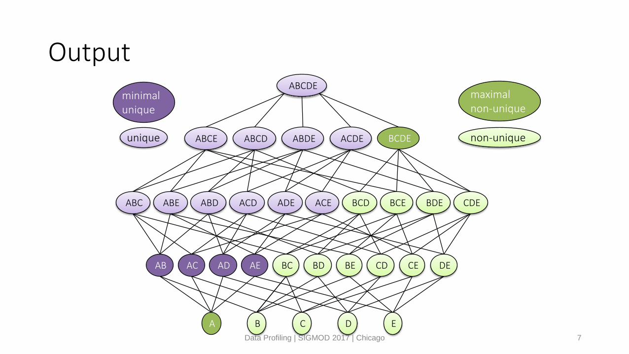
Data Profiling | SIGMOD 2017 | Chicago 7
A B C D E
AB AC AD AE BC BD BE CD CE DE
ABC ABDABE ACD ACEADE BCD BCE BDE CDE
ABCDABCE ABDE ACDE BCDE
ABCDEminimal unique
unique
maximalnon-unique
non-unique

TPCH line item
Data Profiling | SIGMOD 2017 | Chicago 8
unique non-unique
8 columns
9 columns
10 columns

Pruning
• Pruning: • If X is unique, its supersets must be unique• If Y is non-unique, its subsets must be non-unique
• Finding a unique column prunes half the lattice• Remove column from initial data set and restart
Data Profiling | SIGMOD 2017 | Chicago 9

Pruning effect of attribute pair
Data Profiling | SIGMOD 2017 | Chicago 10
A B C D E
AB AC AD AE BC BD BE CD CE DE
ABC ABDABE ACD ACEADE BCD BCE BDE CDE
ABCDABCE ABDE ACDE BCDE
ABCDEminimal unique
unique

Pruning both ways
Data Profiling | SIGMOD 2017 | Chicago 11A B C D E
AB AC AD AE BC BD BE CD CE DE
ABC ABDABE ACD ACEADE BCD BCE BDE CDE
ABCDABCE ABDE ACDE BCDE
ABCDEminimal unique
unique
maximalnon-unique
non-unique

Discovery Algorithms
Data Profiling | SIGMOD 2017 | Chicago 12
Row-basedColumn-based
Bottom up HybridTop down
GordianAprioriHCA DUCC
Unique column combination discovery
SWAN

Column-based algorithms
• Traverse through lattice• Check for uniqueness
• Can use database backend• SELECT COUNT(DISTINCT A, B, C) FROM R• Compare with row-count
• Prune lattice accordingly
Data Profiling | SIGMOD 2017 | Chicago 13

Apriori-based[Giannella, Wyss: Finding minimal keys in a relation instance. (1999)]
• Basic idea: • Using the state of combinations of size k• We need to visit only unpruned combinations of size k+1• Add non-unique columns to combination of size k
• Start with individual columns• Check pairs of non-unique columns• Check triples of non-unique pairs …• Terminate if no new combinations can be enumerated
Data Profiling | SIGMOD 2017 | Chicago 14

Apriori visualized
Data Profiling | SIGMOD 2017 | Chicago 15
A B C D E
AB AC AD AE BC BD BE CD CE DE
ABC ABDABE ACD ACEADE BCD BCE BDE CDE
ABCDABCE ABDE ACDE BCDE
ABCDEminimal unique
unique
maximalnon-unique
non-unique
A B C D E
AB AC AD AE BC BD BE CD CE DE
ABC ABDABE ACD ACEADE BCD BCE BDE CDE
ABCDABCE ABDE ACDE BCDE
ABCDE

Characteristics of Apriori
• Works well for small uniques• Bottom-up checks single columns first
• Best case: all columns are unique• n checks
• Worst case: no uniques = one duplicate row• 2n checks
• Apriori is exponential in n
Data Profiling | SIGMOD 2017 | Chicago 16

Extensions
• Top-down• Start from top (all columns)• Works well if solution set is high up
• Hybrid[Giannella, Wyss: Finding minimal keys in a relation instance. (1999)]
• Interleaved bottom-up and top-down• Works well if solution set has many small and large combinations• Worst case: solution set in the middle
• Statistics-based extensions [Abedjan, Naumann: Advancing the discovery of unique column combinations, CIKM’11]
• Uses histograms for pruning• Random walk [Heise, Quiané-Ruiz, Abedjan, Jentzsch, Naumann: Scalable Discovery of Unique Column Combinations, PVLDB’14]
• Pick random superset if current column set is non-unique, random subset otherwise
Data Profiling | SIGMOD 2017 | Chicago 17

A B C D E
AB AC AD AE BC BD BE CD CE DE
ABC ABD ABE ACD ACE ADE BCD BCE BDE CDE
ABCD ABCE ABDE ACDE BCDE
ABCDE
ABCD
ABC
ABCE
ABD
ABDE
AB
ACD
CD
ACD BCD CDE
Unique column combination
Minimal unique column combination
Non-unique column combination
Maximal non-unique column combination
Pruned
Visited nodes: 10 out of 26
Data Profiling | SIGMOD 2017 | Chicago 18
ACD and BCD are minimal uniques

Uniques on Dynamic Data: SWAN[Abedjan, Quanie-Ruiz, Naumann: Detecting Unique Column Combinations on Dynamic Data, ICDE’14]
• Inserts may create new duplicate combinations• Minimal uniques might become non-unique• Maximal non-uniques might lose maximality
• Deletes remove duplicate value combinations• Non-uniques might become unique• Minimal uniques might lose minimality
• SWAN• Leverage previously discovered minimal uniques and maximal non-uniques• Create appropriate indices
Data Profiling | SIGMOD 2017 | Chicago 19

Functional Dependencies
Data Profiling | SIGMOD 2017 | Chicago 20
Game of Dependencies

Trivial and minimal FDs
• „X → A“ is a statement about a relation R: When two tuples have same value in attribute set X, the must have same values in attribute A.
• Non-trivial: At least one attribute on RHS does not appear on LHS• Street, City → Zip, City
• Completely non-trivial: Attributes on LHS and RHS are disjoint.• Street, City → Zip
• Minimal FD: RHS does not depend on any subset of LHS
• Typical goal: Given a relation R, find all minimal completely non-trivial functional dependencies.
Data Profiling | SIGMOD 2017 | Chicago 21

Naive Discovery Approach• Task: Given relation R, detect all minimal, non-trivial FDs X → A.
• For each A ∈ R• For each column combination X in R\A
• If COUNT DISTINCT(X) = COUNT DISTINCT(XA)• Return X → A
• Complexity• For each of the |R| possibilities for RHS
• check 2( 𝑅𝑅 −1) combinations for LHS
Data Profiling | SIGMOD 2017 | Chicago 22

FD Discovery approaches
Data Profiling | SIGMOD 2017 | Chicago 23
FD Discovery CFD Discovery
Column-based
Row-based
TANE
FUN
FD_Mine
Dep-Miner
FastFDs
Other FDEP
CTANE
FastCFD
Chiang & Miller
DFD & HyFD

TANE [Huhtala, Kärkkäinen, Porkka, Toivonen:TANE: An Efficient Algorithm for Discovering Functional and Approximate Dependencies,
Computer Journal’99]
• Bottom up traversal through lattice• ⇒ only minimal dependencies• Pruning: if B→C, don’t check BD→C• Avoids COUNT DISTINCTs
• For a set X, test all X\A → A, A∈X• ⇒ only non-trivial dependencies
Data Profiling | SIGMOD 2017 | Chicago 24
A B C D
AB ACAD BC BD CD
ABC ABD ACD BCD
ABCD

Candidate Sets
• RHS candidate set C(X)• Stores only those attributes that might depend on all other attributes in X.
• I.e., those that still need to be checked• If A∈C(X) then A does not depend on any proper subset of X.
• C(X) = R \ {A∈X | X\A → A holds}• Examples: R= {ABCD}, and A → C and CD → B hold
• C(A) = {ABCD}\{} = C(B) = C(C) = C(D)• C(AB) = {ABCD}\{}• C(AC) = {ABCD}\{C} = {ABD}• C(CD) = {ABCD}\{}• C(BCD) = {ABCD}\{B} = {ACD}
Data Profiling | SIGMOD 2017 | Chicago 25

RHS Candidate Pruning
• RHS candidates: C+(X) = {A∈R | ∀B∈X: X\{A,B} → B does not hold}• Special case: A = B corresponds to C(X)
• Reminder: C(X) = R \ {A∈X | X\A → A holds}
• This definition removes three types of candidates:• Minimality• Pseudotransitivity• Superkey
• Examples: R= {ABCD}, and A → C and CD → B hold• C(ABC) = {A}• C(BCD) = {ACD}
Data Profiling | SIGMOD 2017 | Chicago 26
A B C D
AB ACAD BC BD CD
ABC ABD ACD BCD
ABCD

Row-Based Algorithms
Data Profiling | SIGMOD 2017 | Chicago 27
• For each candidate RHS (say, phone)• Find difference sets including phone, with phone
removed• {first,last,age}, {fist,age}, {age}, {last}, {first,last}
• So there are pairs of tuples with different phones and different {first,last,age}, different {first,age}, etc.
• Find minimal column subsets that have a non-empty intersection with each difference set
• {last,age}
• Conclude that {last,age} phone

FD Discovery on Dynamic Data [Wang, Tsou, Lin and Hong: Maintenance of discovered functional dependencies: Incremental deletion, ISDA’03]
• Insertions• Existing FDs may be violated: Check each one
• Deletions• New FD may appear if conflicting tuple deleted: Revisit entire lattice
Data Profiling | SIGMOD 2017 | Chicago 28

Order Dependencies
Data Profiling | SIGMOD 2017 | Chicago 29

Example
• XA if sorting on X also sorts on A
• taxsalary• ODs subsume FDs
• If X functionally determines Y then X orders XY
Data Profiling | SIGMOD 2017 | Chicago 30

Discovering Order Dependencies
• List-based lattice approach [Langer, Naumann: Discovering Order Dependencies, VLDBJ’15]
• Apriori-like, but order matters: XYA is different from YXA
• Set-based lattice approach [Szlichta, Godfrey, Golab, Kargar, Srivastava: Effective and Complete Discovery of Order Dependencies via Set-based Axiomatization, PVLDB’17]
• Rewrite ODs using a set-based canonical form
• Both approaches:• New pruning rules based on OD semantics/axioms
Data Profiling | SIGMOD 2017 | Chicago 31

Inclusion Dependencies
Data Profiling | SIGMOD 2017 | Chicago 32

BINDER – divide & conquer based IND detection
Linking web tables – an example
Web Data Commons ProjectData Profiling | SIGMOD 2017 | Chicago 33
Planet Synodic period Synodic period (mean) Days in retrogradeMercury 116 3.8 ~21
Venus 584 19.2 41Mars 780 25.6 72
Jupiter 399 13.1 121Saturn 378 12.4 138
Uranus 370 12.15 151Neptune 367 12.07 158
Name Type Equatorialdiameter Mass Orbital
radiusOrbitalperiod
Rotationperiod
Confirmedmoons Rings Atmosphere
Mercury
Terrestrial 0.382 0.06 0.47 0.24 58.64 0 no minimal
Venus Terrestrial 0.949 0.82 0.72 0.62 −243.02 0 no CO2, N2
Earth Terrestrial 1.000 1.00 1.00 1.00 1.00 1 no N2, O2, Ar
Mars Terrestrial 0.532 0.11 1.52 1.88 1.03 2 no CO2, N2, Ar
Jupiter Giant 11.209 317.8 5.20 11.86 0.41 67 yes H2, He
Saturn Giant 9.449 95.2 9.54 29.46 0.43 62 yes H2, He
Uranus Giant 4.007 14.6 19.22 84.01 −0.72 27 yes H2, He
Neptune Giant 3.883 17.2 30.06 164.8 0.67 14 yes H2, He
Planet Mean distance Relative mean distanceMercury 57.91 1
Venus 108.21 1.86859Earth 149.6 1.3825Mars 227.92 1.52353Ceres 413.79 1.81552
Jupiter 778.57 1.88154Saturn 1,433.53 1.84123
Uranus 2,872.46 2.00377Neptune 4,495.06 1.56488
Pluto 5,869.66 1.3058
Symbol Unicode GlyphSun U+2609 ☉
Moon U+263D ☽Moon U+263E ☾
Mercury U+263F ☿Venus U+2640 ♀Earth U+1F728 🜨🜨Mars U+2642 ♂
Jupiter U+2643 ♃Saturn U+2644 ♄
Uranus U+2645 ♅Uranus U+26E2 ⛢
Neptune U+2646 ♆Eris ≈ U+2641 ♁Eris ≈ U+29EC ⧬
Pluto U+2647 ♇Pluto not present --Aries U+2648 ♈
Taurus U+2649 ♉Gemini U+264A ♊Cancer U+264B ♋
Leo U+264C ♌Virgo U+264D ♍Libra U+264E ♎
Scorpio U+264F ♏Sagittarius U+2650 ♐Capricorn U+2651 ♑Capricorn U+2651 ♑Aquarius U+2652 ♒
Pisces U+2653 ♓Conjunction U+260C ☌
... ... ...
Sign House Domicile Detriment Exaltation Fall Planetary Joy
Aries 1st House Mars Venus Sun Saturn Mercury
Taurus 2nd House Venus Pluto Moon Uranus Jupiter
Gemini 3rd House Mercury Jupiter N/A N/A Saturn
Cancer 4th House Moon Saturn Jupiter Mars Venus
Leo 5th House Sun Uranus Neptune Mercury Mars
Virgo 6th House Mercury NeptunePluto,
Mercury Venus Saturn
Libra 7th House Venus Mars Saturn Sun Moon
Scorpio 8th House Pluto Venus Uranus Moon Saturn
Sagittarius 9th House Jupiter Mercury N/A N/A Sun
Capricorn10th
House Saturn Moon Mars Jupiter Mercury
Aquarius11th
House Uranus Sun Mercury Neptune Venus
Planet Rotation Period
Revolution Period
Mercury 58.6 days 87.97 days
Venus 243 days 224.7 daysEarth 0.99 days 365.26 daysMars 1.03 days 1.88 years
Jupiter 0.41 days 11.86 yearsSaturn 0.45 days 29.46 years
Uranus 0.72 days 84.01 yearsNeptun
e 0.67 days 164.79 yearsPluto 6.39 days 248.59 years
Planet Calculated (in AU)
Observed(in AU)
Perfect octaves
Actual distance
Mercury 0.4 0.387 0 0Venus 0.7 0.723 1 1.1Earth 1 1 2 2Mars 1.6 1.524 4 3.7
Asteroid belt 2.8 2.767 8 7.8
Jupiter 5.2 5.203 16 15.7Saturn 10 9.539 32 29.9
Uranus 19.6 19.191 64 61.4Neptune 38.8 30.061 96 -96.8
Pluto 77.2 39.529 128 127.7http://webdatacommons.org/webtables/index.html
Planet Synodic period Synodic period (mean) Days in retrogradeMercury 116 3.8 ~21
Venus 584 19.2 41Mars 780 25.6 72
Jupiter 399 13.1 121Saturn 378 12.4 138
Uranus 370 12.15 151Neptune 367 12.07 158
Name Type Equatorialdiameter Mass Orbital
radiusOrbitalperiod
Rotationperiod
Confirmedmoons Rings Atmosphere
Mercury
Terrestrial 0.382 0.06 0.47 0.24 58.64 0 no minimal
Venus Terrestrial 0.949 0.82 0.72 0.62 −243.02 0 no CO2, N2
Earth Terrestrial 1.000 1.00 1.00 1.00 1.00 1 no N2, O2, Ar
Mars Terrestrial 0.532 0.11 1.52 1.88 1.03 2 no CO2, N2, Ar
Jupiter Giant 11.209 317.8 5.20 11.86 0.41 67 yes H2, He
Saturn Giant 9.449 95.2 9.54 29.46 0.43 62 yes H2, He
Uranus Giant 4.007 14.6 19.22 84.01 −0.72 27 yes H2, He
Neptune Giant 3.883 17.2 30.06 164.8 0.67 14 yes H2, He
Planet Mean distance Relative mean distanceMercury 57.91 1
Venus 108.21 1.86859Earth 149.6 1.3825Mars 227.92 1.52353Ceres 413.79 1.81552
Jupiter 778.57 1.88154Saturn 1,433.53 1.84123
Uranus 2,872.46 2.00377Neptune 4,495.06 1.56488
Pluto 5,869.66 1.3058
Symbol Unicode GlyphSun U+2609 ☉
Moon U+263D ☽Moon U+263E ☾
Mercury U+263F ☿Venus U+2640 ♀Earth U+1F728 🜨🜨Mars U+2642 ♂
Jupiter U+2643 ♃Saturn U+2644 ♄
Uranus U+2645 ♅Uranus U+26E2 ⛢
Neptune U+2646 ♆Eris ≈ U+2641 ♁Eris ≈ U+29EC ⧬
Pluto U+2647 ♇Pluto not present --Aries U+2648 ♈
Taurus U+2649 ♉Gemini U+264A ♊Cancer U+264B ♋
Leo U+264C ♌Virgo U+264D ♍Libra U+264E ♎
Scorpio U+264F ♏Sagittarius U+2650 ♐Capricorn U+2651 ♑Capricorn U+2651 ♑Aquarius U+2652 ♒
Pisces U+2653 ♓Conjunction U+260C ☌
... ... ...
Sign House Domicile Detriment Exaltation Fall Planetary Joy
Aries 1st House Mars Venus Sun Saturn Mercury
Taurus 2nd House Venus Pluto Moon Uranus Jupiter
Gemini 3rd House Mercury Jupiter N/A N/A Saturn
Cancer 4th House Moon Saturn Jupiter Mars Venus
Leo 5th House Sun Uranus Neptune Mercury Mars
Virgo 6th House Mercury NeptunePluto,
Mercury Venus Saturn
Libra 7th House Venus Mars Saturn Sun Moon
Scorpio 8th House Pluto Venus Uranus Moon Saturn
Sagittarius 9th House Jupiter Mercury N/A N/A Sun
Capricorn10th
House Saturn Moon Mars Jupiter Mercury
Aquarius11th
House Uranus Sun Mercury Neptune Venus
Planet Rotation Period
Revolution Period
Mercury 58.6 days 87.97 days
Venus 243 days 224.7 daysEarth 0.99 days 365.26 daysMars 1.03 days 1.88 years
Jupiter 0.41 days 11.86 yearsSaturn 0.45 days 29.46 years
Uranus 0.72 days 84.01 yearsNeptun
e 0.67 days 164.79 yearsPluto 6.39 days 248.59 years
Planet Calculated (in AU)
Observed(in AU)
Perfect octaves
Actual distance
Mercury 0.4 0.387 0 0Venus 0.7 0.723 1 1.1Earth 1 1 2 2Mars 1.6 1.524 4 3.7
Asteroid belt 2.8 2.767 8 7.8
Jupiter 5.2 5.203 16 15.7Saturn 10 9.539 32 29.9
Uranus 19.6 19.191 64 61.4Neptune 38.8 30.061 96 -96.8
Pluto 77.2 39.529 128 127.7

Unary IND detection complexity
Data Profiling | SIGMOD 2017 | Chicago 34
Name Type Equatorialdiameter Mass Orbital
radiusOrbitalperiod
Rotationperiod
Confirmedmoons Rings Atmosphere
Mercury Terrestrial 0.382 0.06 0.47 0.24 58.64 0 no minimalVenus Terrestrial 0.949 0.82 0.72 0.62 −243.02 0 no CO2, N2
Earth Terrestrial 1.000 1.00 1.00 1.00 1.00 1 no N2, O2, ArMars Terrestrial 0.532 0.11 1.52 1.88 1.03 2 no CO2, N2, Ar
Jupiter Giant 11.209 317.8 5.20 11.86 0.41 67 yes H2, HeSaturn Giant 9.449 95.2 9.54 29.46 0.43 62 yes H2, He
Uranus Giant 4.007 14.6 19.22 84.01 −0.72 27 yes H2, HeNeptune Giant 3.883 17.2 30.06 164.8 0.67 14 yes H2, He
■ Name ⊆ Type ?
■ Name ⊆ Equatorial_diameter ?
■ Name ⊆ Mass ?
■ Name ⊆ Orbital_radius ?
■ Name ⊆ Orbital_period ?
■ Name ⊆ Rotation_period ?
■ Name ⊆ Confirmed_moons ?
■ Name ⊆ Rings ?
■ Name ⊆ Atmosphere ?
■ Type ⊆ Name ?
■ Type ⊆ Equatorial_diameter ?
■ Type ⊆ Mass ?
■ Type ⊆ Orbital_radius ?
■ Type ⊆ Orbital_period ?
■ Type ⊆ Rotation_period ?
■ Type ⊆ Confirmed_moons ?
■ Type ⊆ Rings ?
■ Type ⊆ Atmosphere ?
■ Mass ⊆ Name ?
■ Mass ⊆ Type ?
■ Mass ⊆ Equatorial_diameter ?
■ …
Complexity: O(n2-n) for n attributes
Example:10 attr ~ 90 checks1,000 attr ~ 999,000 checks

MIND[Marchi, Lopes, Petit: Unary and n-ary inclusion dependency discovery in relational databases,JIIS’09]
Data Profiling | SIGMOD 2017 | Chicago 35
acajjiefha
A
bbcgbcigii
B
geggafgfaa
C
dbbbddhddb
D
egbbegegbg
E
hicaajacci
F G
cbbcfbcjdd
Rel. 1 Rel. 2a
b
c
d
e
f
g
h
i
j
A
B
A
B
A
A
B
A
A
A
C
D
B
D
C
C
C
D
B
F
F
E
F
G
E
G
E
F
F
G
G
G
F ⊆ A
Needs to fit in main memory!
All intersections are checked, but not all are necessary!
Xattributesdataflow
valuesignored

BINDER[Papenbrock, Quiane, Naumann: Divide & Conquer-based Inclusion Dependency Discovery, PVLDB’15]
Data Profiling | SIGMOD 2017 | Chicago 36
a
A
b
Ba
C
b
D
b
Ea
F
b
G
c cd d
c cd
ef
ef
ef
hg g g
h
ij
i ij j
A B C D E F G
X X
X X X X
X X X X
X X X X X
F ⊆ A
h
acajjiefha
A
bbcgbcigii
B
geggafgfaa
C
dbbbddhddb
D
egbbegegbg
E
hicaajacci
F G
cbbcfbcjdd
Divide
Rel. 1 Rel. 2
ConquerX
attributesdataflow
valuesignored
validation?
Dynamic Memory Handling:Spill largest buckets to disk if
memory is exhausted.
Lazy Partition Refinement:Split a partition if it does not
fit into main memory.

Extensions
• Dependencies are sensitive to data errors• Conditional Functional Dependencies
• XA but only for X=x1 and X=x5
• Approximate Functional Dependencies• How many rows (at a minimum) would have
to be removed so the remaining rows satisfy the FD?
• Metric Functional Dependencies• XA holds if tuples that agree on X have As
within some distance
Data Profiling | SIGMOD 2017 | Chicago 37
[Caruccio, Deufemia, Polese: Relaxed Functional Dependencies - A Survey of Approaches. TKDE ’16]

Visualization[1011066.Name] =] [1011057.Name] [129284.Reference] =] [1223862.null] [586920.Ref.] [1030730.RCDB page] [108435.No.] [1248790.Source] [983315.References] [207338.Home railway
(external link)] [975850.Ref] [1375996.Source] [1129539.References] [1168707.References] [744488.Ref] [1169311.Ref] [1068498.Ref] [163214.Reference] [604676.References] [1002900.Ref] [749972.Reference] [951640.References] [939700.Page] [900853.Ref] [788203.Ref] [788409.References] [978758.Ref] [652885.Link] [652377.Ref] [1320358.Reference] [1287392.Ref] [1012269.Report] [1180077.References] [1274408.Ref] [856227.NFL Recap] [1286480.Ref] [1354142.null] [525501.References] [630016.Notes] [762537.Refs] [902406.Report] [1005369.Link] [1255682.Source] [1157534.Source] [1065320.Ref] [956840.Ref] [775466.References] [988811.Ref] [1005838.Link] [1005593.Link] [576411.References] [1134428.Ref] [1170953.Reference(s)] [699144.Note] [268733.References] [931606.Notes] [1284557.Ref.] [1357973.Source] [1238931.Report] [867400.Reference] [794774.Ref] [716064.Refs] [377521.References] [995370.Ref] [1282132.References] [1358158.Ref.] [1120007.Ref] [1342522.Ref] [1319381.null] [889114.Ref] [1004839.Link] [697527.Website] [980509.Ref(s)] [1078901.Ref]
[1390416.Rank] =] [1169921.Rank] [1183098.Rank] [1011765.Rank] [1225076.Rank] [454782.Rank] [1186535.Rank] [1209635.Rank] [1161665.Rank] [708465.Rank] [708648.Rank]
[637307.Date] =] [1311505.Date] [1337020.Date] [1083420.Event] =] [976659.Event] [976901.Event] [975917.Event] [1060037.Event] [1068182.Event] [1067251.Event] [1067097.Event] [1000067.Event]
[972968.Event] [1058267.Event] [988323.Event] [1003312.Event] [1063506.Event] [1027145.Event] [1078507.Event] [1062268.Event][302006.Role:] =] [391330.Role:] [703281.Role:] [387497.Role:] [735612.Role:] [151885.Role:] [150598.Role:] [1083410.Event] =] [983546.Event] [975773.Event] [1071989.Event] [1068219.Event] [1002900.Event] [1074984.Event] [967160.Event] [1052352.Event]
[1066949.Event] [1082562.Event] [1151162.Event] [1042660.Event] [1056643.Event] [950860.Event] [958921.Event] [1063309.Event][973967.Event] [1027145.Event] [1062263.Event]
[73362.State] =] [1185141.State] [1083402.Event] =] [1083339.Event] [1068498.Event] [1060027.Event] [1002823.Event] [1046135.Event] [1249836.Event] [1000145.Event]
[994576.Event] [990543.Event] [854590.Venue] =] [883202.Venue] [890993.Venue] [1104659.Venue] [648260.TEAM] =] [1286540.Club] [1308745.Club] [627822.Division Record] =] [466958.Sets W - L] [1236345.Match] =] [1231569.Match] ...
Data Profiling | SIGMOD 2017 | Chicago

Visualization
INDs = {R1.A ⊆ R2.B,R3.A ⊆ R1.D,R3.C ⊆ R2.A,R3.B ⊆ R4.A
}
G= (V = {
R1, R2, R3, R4},
E = {(R1, R2), (R3, R1),(R3, R2), (R3, R4)
}
)
Data Profiling | SIGMOD 2017 | Chicago

Visualization
make G undirected
find Connected
components
Data Profiling | SIGMOD 2017 | Chicago

Interactive Front End

Ranking Dependencies• Uniques/FDs/ODs
• rank by size of left hand side (XA over XYZWA)• rank by position in schema• note: apriori-like approaches naturally produce “small” dependencies first
• Inclusion dependencies• rank by syntactic similarity: (name ⊆ cust_name)• rank by overlap (given A ⊆ B, compute |B/A|)
• Approximate dependencies• rank by how many rows satisfy them
• Conditional dependencies• rank by support (how many rows they cover)
Data Profiling | SIGMOD 2017 | Chicago

More Dependencies• Denial constraints [Chu, Ilyas, Papotti: Discovering denial constraints, PVLDB’13]
• First order logic• E.g., If two people live in the same province, the one earning a lower salary must
pay less tax• Differential dependencies [Song and Chen: Differential dependencies: Reasoning and discovery, TODS, 2011]
• XY holds when any pair of tuples whose X values are close also have Y values which are close
• Sequential dependencies [Golab, Karloff, Korn, Saha, Srivastava: Sequential dependencies, PVLDB’09]
• X[p,q] A holds if sorting by X also sorts by A, and consecutive A values are at least p and at most q apart
• E.g., Year [0,1000] Salary means that salaries do not decrease over time and increase by at most 1000/year
next slide deck

Tutorial Overview• Motivation
• Task classification• Use cases
• Tools• Research and industry• Shortcomings
• Single and Multiple Column Analysis• Cardinalities and datatypes• Co-occurrences and summaries
• Dependencies• UCCs, FDs, ODs, INDs• and their discovery algorithms
• Outlook• Functionality• Semantics
Data Profiling | SIGMOD 2017 | Chicago 2

Part Overview
• Functional challenges• Non-functional challenges• Semantics of Dependencies
Data Profiling | SIGMOD 2017 | Chicago 3

Data Profiling | SIGMOD 2017 | Chicago 4
Extending the Functionalityof Data Profiling

Many Other Kinds of Dependencies
Data Profiling | SIGMOD 2017 | Chicago 5[Abiteboul, Hull, Vianu: Foundations of Databases, 1995]

Extended Classification of Profiling Tasks
Data Profiling | SIGMOD 2017 | Chicago 6
Data Profiling
Single source
Single column
Cardinalities
Uniqueness and keys
Patterns and data types
Distributions
Multiple columns^^
Uniqueness and keys
Inclusion and foreign key dep.
Functional dependencies
Conditional and approximate
dep.
Multiple sources
Data overlap
Duplicate detection
Record linkage
Schematic overlap
Schema matching
Cross-schema dependencies
Topical overlap
Topic discovery
Topical clustering

Profiling for Integration
• Create measures to estimate integration (and cleansing) effort• Schema and data overlap• Severity of heterogeneity
• Schema matching/mapping• What constitutes the “difficulty”
of matching/mapping?• Duplicate detection
• Estimate data overlap• Estimate fusion effort
• Overall: Determine integration complexity and integration effort• Intrinsic complexity: Schema and data• Extrinsic complexity: Tools and expertise
Data Profiling | SIGMOD 2017 | Chicago 7

Integration Effort Estimation
Data Profiling | SIGMOD 2017 | Chicago 8
SS
I
T
J
Schema analysis
(matching)
Complexity model
Effort model
Data analysis (profiling)
Measured effort
Integration tools(mapping & ETL)
Tool capabilities
Integration specialist
Production side Estimation side
Integration result
Estimatedeffort
[Kruse, Papotti, Naumann: Estimating Data Integration and Cleaning Effort. EDBT 2015]

Profiling new Types of Data
• Traditional data profiling: Single table or multiple tables• More and more data in other models
• XML / nested relational / JSON• RDF triples• Textual data: Blogs, Tweets, News• Multimedia data
• Different models offer new dimensions to profile• XML: Nestedness, measures at different nesting levels• RDF: Graph structure, in- and outdegrees• Multimedia: Color, video-length, volume, etc.• Text: Sentiment, sentence structure, complexity, and other linguistic measures
Data Profiling | SIGMOD 2017 | Chicago 9

Example: Text Profiling
• Statistical measures• Syllables per word• Sentence length• Proportions of parts of speech
• Vocabulary measures• Frequencies of specific words• Type-token ratio• Simpson’s index (vocabulary richness)• Number of hapax (dis)legomena
• Token that occurs exactly once (twice) in the corpus• Characterize style of an author
Data Profiling | SIGMOD 2017 | Chicago 10

Average Sentence Length
Data Profiling | SIGMOD 2017 | Chicago 11[Keim and Oelke: Literature Fingerprinting: A New Method for Visual Literary Analysis. IEEE VAST 2007]

Hapax Legomena
Data Profiling | SIGMOD 2017 | Chicago 12[Keim and Oelke: Literature Fingerprinting: A New Method for Visual Literary Analysis. IEEE VAST 2007]

Verse Length
Data Profiling | SIGMOD 2017 | Chicago 13[Keim and Oelke: Literature Fingerprinting: A New Method for Visual Literary Analysis. IEEE VAST 2007]

Example: News Article Statistics
Data Profiling | SIGMOD 2017 | Chicago 14

Data Profiling | SIGMOD 2017 | Chicago 15
Improving Non-Functional Propertiesof Data Profiling

Holistic Profiling
• Various profiling methods for various profiling tasks• Commonalities/similarities
• Search space: All column combinations (or pairs thereof)• I/O: Read all data at least once• Data structure: Some index or hash table• Pruning and candidate generation: based on subset/superset relationships• Sortation: Benefit from sorted sets
• Challenge: Develop single method to output all/most profiling results
Data Profiling | SIGMOD 2017 | Chicago 16

Incremental Profiling
• Data is dynamic• Insert (batch or tuple-based)• Updates• Deletes
• Problem: Keep profiling results up-to-date without reprofiling the entire data set
• Easy examples: SUM, MIN, MAX, COUNT, AVG• Difficult examples: MEDIAN, uniqueness, FDs, etc.
Data Profiling | SIGMOD 2017 | Chicago 17

Online Profiling• Profiling is long procedure
• Boring for developers• Expensive for machines (I/O and CPU)
• Challenge: Display intermediate results• … of improving/converging accuracy• Allows early abort of profiling run
• Gear algorithms toward that goal• Allow intermediate output• Enable early output: “progressive” profiling
Data Profiling | SIGMOD 2017 | Chicago 18

Temporal Profiling
• Observe behavior of dependencies over time• Do FDs appear and disappear?• Does a partial IND become less partial over time?• …
• Metadata monitoring• Meta-Metadata
Data Profiling | SIGMOD 2017 | Chicago 19

Profiling Query Results
• Query results are boring: Spruce them up with some metadata
• Usually only: Row count• For each column, give some statistics
• Idea: Piggy-back profiling on query execution
• Re-use sortations, hash tables, etc.
Data Profiling | SIGMOD 2017 | Chicago 20
Data Generation and Testing
• Generate volumes of data with certain properties• Test extreme cases• Test scalability
• Problem: Interaction between properties• FDs vs. uniqueness• Patterns vs. conditional INDs• Distributions vs. all others…
• Problem: Create realistic data• Distributions, patterns• Placement of dependencies (tight or spread out)
Data Profiling | SIGMOD 2017 | Chicago 21
Recent work[Arocena et al. : Messing Up with BART: Error Generation for Evaluating Data-Cleaning Algorithms. PVLDB 9(2), 2015][Arocena et al. : The iBench Integration Metadata Generator . PVLDB 9(3), 2015]

Data Profiling Benchmark
• Define data• Data generation• Real-world dataset(s)• Different scale-factors: Rows and columns
• Define tasks• Individual tasks• Sets of tasks
• Define measures• Speed• Speed/cost• Minimum hardware requirements• Accuracy for approximate approaches
Data Profiling | SIGMOD 2017 | Chicago 22

Summary – much to do
• Efficient profiling• Scalable profiling• Holistic profiling• Incremental profiling• Online profiling• Temporal profiling• Profiling query results• Profiling new types of data• Data profiling benchmark
Data Profiling | SIGMOD 2017 | Chicago 23

Data Profiling | SIGMOD 2017 | Chicago 24
Semantic Interpretation of Profiling Results

Turning Instance-based Observations to Schema-based Constraints• Hundreds of UCCs – which ones are keys?• Thousands of FDs – which ones are true?• Millions of INDs – which ones are foreign keys?
• User-driven interpretation • Rank and visualize metadata
• Machine-driven interpretation• Machine learning
Data Profiling | SIGMOD 2017 | Chicago 25

Thanks to co-authors, colleagues and team!
• Carl Ambroselli (Metanome, HPI)• Jana Bauckmann (INDs, HPI)• Tanja Bergmann (Metanome, HPI)• Jens Ehrlich (cUCCs, HPI)• Claudia Exeler (Metanome, HPI)• Moritz Finke (Metanome, HPI)• Toni Gruetze (ProLOD, HPI)• Hazar Harmouch (Cardinalities, HPI)• Arvid Heise (UCCs, HPI)
• Anja Jentzsch(ProLOD, HPI)• Sebastian Kruse (INDs, Metadata Store,
HPI)• Philipp Langer (ODs, HPI)• Thorsten Papenbrock (INDs, FDs,
Metanome, HPI)• Paolo Papotti (Profiling for Integration,
ASU)• Jorge Quiané-Ruiz (UCCs, QCRI)• Patrick Schulze (FDs, HPI)• Fabian Tschirschnitz (INDs, HPI)• Jakob Zwiener (Metanome, HPI)
Data Profiling | SIGMOD 2017 | Chicago 26

Summary
Data Profiling | SIGMOD 2017 | Chicago 27
Data Profiling
Single source
Single column
Cardinalities
Uniqueness and keys
Patterns and data types
Distributions
Multiple columns
Uniqueness and keys
Inclusion and foreign key dep.
Functional dependencies
Conditional and approximate
dep.
Multiple sources
Topical overlap
Topic discovery
Topical clustering
Schematic overlap
Schema matching
Cross-schema dependencies
Data overlap
Duplicate detection
Record linkage
Slides are available at https://hpi.de/naumann/publications/selected-presentations.html