data quality objectives for pm continuous methods ii · be performed using the dqo measurement e...
TRANSCRIPT

TR-CAN-04-02 June 2004
Data Quality Objectives forPM Continuous Methods II
Prepared for
National Exposure Research LaboratoryU.S. Environmental Protection Agency
Research Triangle Park, NC 27711
Contract 68-D-00-206
ManTech Environmental Technology, Inc., TeamP.O. Box 12313
Research Triangle Park, NC 27709
A ManTech International Company
TR-CAN-04-02 June 2004
Data Quality Objectives forPM Continuous Methods II
by
Paul Mosquin and Frank McElroyResearch Triangle Institute
ManTech Team
ManTech Environmental Technology, Inc.Research Triangle Park, NC 27709
Prime Contractor
Research Triangle InstituteResearch Triangle Park, NC 27709
Subcontractor
Submitted to
Elizabeth Hunike, Contracting Officer’s RepresentativeProcess Modeling Research Branch
Human Exposure and Atmospheric Sciences DivisionNational Exposure Research LaboratoryU.S. Environmental Protection Agency
Research Triangle Park, NC 27711
Contract 68-D-00-206
Reviewed and approved by
Frank McElroy Christopher NoblePrincipal Investigator RTI Technical Supervisor
ManTech Environmental Technology, Inc.P.O. Box 12313
Research Triangle Park, NC 27709

TR-CAN-04-02
iii
Foreword
This technical report presents the results of work performed by ManTech EnvironmentalTechnology, Inc., and RTI International under Contract 68-D-00-206 for the Human Exposure andAtmospheric Sciences Division, National Exposure Research Laboratory, U.S. EnvironmentalProtection Agency, Research Triangle Park, NC. This technical report has been reviewed byManTech Environmental Technology, Inc., and RTI International and approved for publication.Mention of trade names or commercial products does not constitute endorsement or recommendationfor use.

TR-CAN-04-02
iv
ContentsSection PageForeword . . . . . . . . . . . . . . . . . . . . . . . . . . . . . . . . . . . . . . . . . . . . . . . . . . . . . . . . . . . . . . . . . . . iii
Figures . . . . . . . . . . . . . . . . . . . . . . . . . . . . . . . . . . . . . . . . . . . . . . . . . . . . . . . . . . . . . . . . . . . . . . v
Tables . . . . . . . . . . . . . . . . . . . . . . . . . . . . . . . . . . . . . . . . . . . . . . . . . . . . . . . . . . . . . . . . . . . . . . vi
1 Introduction . . . . . . . . . . . . . . . . . . . . . . . . . . . . . . . . . . . . . . . . . . . . . . . . . . . . . . . . . . . . 1
2 Review of DQO and WA 76 Model . . . . . . . . . . . . . . . . . . . . . . . . . . . . . . . . . . . . . . . . . 3
3 Review of Field Samples . . . . . . . . . . . . . . . . . . . . . . . . . . . . . . . . . . . . . . . . . . . . . . . . . . 5
3.1 Bakersfield Field Data . . . . . . . . . . . . . . . . . . . . . . . . . . . . . . . . . . . . . . . . . . . . . . 5
3.2 Detroit Field Data . . . . . . . . . . . . . . . . . . . . . . . . . . . . . . . . . . . . . . . . . . . . . . . . . 8
3.3 New York Field Data . . . . . . . . . . . . . . . . . . . . . . . . . . . . . . . . . . . . . . . . . . . . . . . 9
3.4 Tampa Field Data . . . . . . . . . . . . . . . . . . . . . . . . . . . . . . . . . . . . . . . . . . . . . . . . . 10
3.5 Winston-Salem Field Data . . . . . . . . . . . . . . . . . . . . . . . . . . . . . . . . . . . . . . . . . . 12
3.6 Conclusions from Field Data . . . . . . . . . . . . . . . . . . . . . . . . . . . . . . . . . . . . . . . . 12
4 Proposed Measurement Error Model . . . . . . . . . . . . . . . . . . . . . . . . . . . . . . . . . . . . . . . 17
5 Performance Bounds for Model Parameters . . . . . . . . . . . . . . . . . . . . . . . . . . . . . . . . . . 19
5.1 Bounds for the Precision, the Intercept, and the Slope . . . . . . . . . . . . . . . . . . . . 19
5.2 Bounds for the Correlation Coefficient . . . . . . . . . . . . . . . . . . . . . . . . . . . . . . . . 22
6 Parameter Estimation . . . . . . . . . . . . . . . . . . . . . . . . . . . . . . . . . . . . . . . . . . . . . . . . . . . . 27
6.1 Maximum Likelihood Estimation . . . . . . . . . . . . . . . . . . . . . . . . . . . . . . . . . . . . 27
6.2 Other Estimators . . . . . . . . . . . . . . . . . . . . . . . . . . . . . . . . . . . . . . . . . . . . . . . . . 27
6.3 Correlation and Its Estimation . . . . . . . . . . . . . . . . . . . . . . . . . . . . . . . . . . . . . . . 29
7 Illustration Using Simulated and Field Data Sets . . . . . . . . . . . . . . . . . . . . . . . . . . . . . . 33
7.1 Model Fit Using Simulated Data . . . . . . . . . . . . . . . . . . . . . . . . . . . . . . . . . . . . . 33
7.2 Model Fit Using Field Data . . . . . . . . . . . . . . . . . . . . . . . . . . . . . . . . . . . . . . . . . 35
8 Discussion . . . . . . . . . . . . . . . . . . . . . . . . . . . . . . . . . . . . . . . . . . . . . . . . . . . . . . . . . . . . 39
9 References . . . . . . . . . . . . . . . . . . . . . . . . . . . . . . . . . . . . . . . . . . . . . . . . . . . . . . . . . . . . 41
Appendix A: R Code for Maximum Likelihood Estimation . . . . . . . . . . . . . . . . . . . . . . . . . . . . 43
Appendix B: Precision and Variance. . . . . . . . . . . . . . . . . . . . . . . . . . . . . . . . . . . . . . . . . . . . . . 45

TR-CAN-04-02
v
FiguresFigure Page1 Time series of days with readings for all four samplers from the Bakersfield
data set . . . . . . . . . . . . . . . . . . . . . . . . . . . . . . . . . . . . . . . . . . . . . . . . . . . . . . . . . . . . . . . . 6
2 Scatterplots of Bakersfield readings for collocated FRM and collocated MetOne BAM samplers . . . . . . . . . . . . . . . . . . . . . . . . . . . . . . . . . . . . . . . . . . . . . . . . . . . 6
3 Scatterplots of Detroit readings for collocated FRM and an R&P TEOM running at 50 °C . . . . . . . . . . . . . . . . . . . . . . . . . . . . . . . . . . . . . . . . . . . . . . . . . . . . . . . . . 8
4 Scatterplot of Detroit TEOM readings vs. FRM readings with points labeled by month . . . . . . . . . . . . . . . . . . . . . . . . . . . . . . . . . . . . . . . . . . . . . . . . . . . . . . . . . . . . . . 9
5 Scatterplots of New York readings for collocated FRM and an R&P TEOM running at 50 °C . . . . . . . . . . . . . . . . . . . . . . . . . . . . . . . . . . . . . . . . . . . . . . . . . . . . . . . . 10
6 Time series of days with complete data for the Tampa site . . . . . . . . . . . . . . . . . . . . . . . 11
7 Scatterplots of Tampa readings for the FRM, the Thermo-Andersen, and the DKK beta gauges . . . . . . . . . . . . . . . . . . . . . . . . . . . . . . . . . . . . . . . . . . . . . . . . . . . . . . . 11
8 Scatterplot of Winston-Salem FRM and R&P TEOM readings . . . . . . . . . . . . . . . . . . . 12
9 Scatterplots illustrating the effect of an unmeasured variable on the correlation . . . . . . 15
10 Allowable multiplicative and additive biases according to the DQO model . . . . . . . . . . 22
11 Left plot is of 100 independent normal N(50,400) variates adjusted for measurement error. Right plot is 100 independent normal N(50,400) variates truncated within [45,55] and then adjusted for measurement error . . . . . . . . . . . . . . . . . 24
12 Simulated sampler readings vs. true daily values for reference samplers and candidate samplers . . . . . . . . . . . . . . . . . . . . . . . . . . . . . . . . . . . . . . . . . . . . . . . . . . . . . . 33
13 Estimated daily values vs. true daily values . . . . . . . . . . . . . . . . . . . . . . . . . . . . . . . . . . 34
TR-CAN-04-02
vi
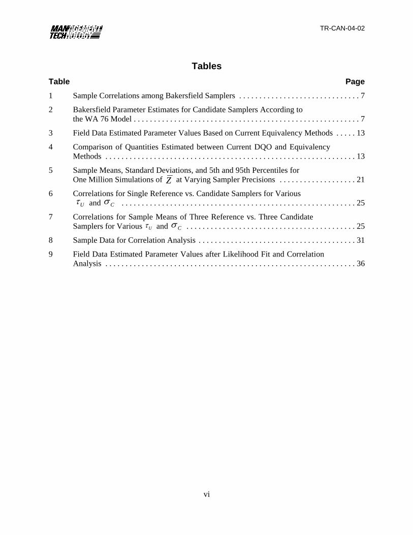
TablesTable Page1 Sample Correlations among Bakersfield Samplers . . . . . . . . . . . . . . . . . . . . . . . . . . . . . . 7
2 Bakersfield Parameter Estimates for Candidate Samplers According to the WA 76 Model . . . . . . . . . . . . . . . . . . . . . . . . . . . . . . . . . . . . . . . . . . . . . . . . . . . . . . . . 7
3 Field Data Estimated Parameter Values Based on Current Equivalency Methods . . . . . 13
4 Comparison of Quantities Estimated between Current DQO and Equivalency Methods . . . . . . . . . . . . . . . . . . . . . . . . . . . . . . . . . . . . . . . . . . . . . . . . . . . . . . . . . . . . . . 13
5 Sample Means, Standard Deviations, and 5th and 95th Percentiles for One Million Simulations of at Varying Sampler Precisions . . . . . . . . . . . . . . . . . . . 21Z
6 Correlations for Single Reference vs. Candidate Samplers for Various and . . . . . . . . . . . . . . . . . . . . . . . . . . . . . . . . . . . . . . . . . . . . . . . . . . . . . . . . . . 25Uτ Cσ
7 Correlations for Sample Means of Three Reference vs. Three Candidate Samplers for Various and . . . . . . . . . . . . . . . . . . . . . . . . . . . . . . . . . . . . . . . . . . 25Uτ Cσ
8 Sample Data for Correlation Analysis . . . . . . . . . . . . . . . . . . . . . . . . . . . . . . . . . . . . . . . 31
9 Field Data Estimated Parameter Values after Likelihood Fit and Correlation Analysis . . . . . . . . . . . . . . . . . . . . . . . . . . . . . . . . . . . . . . . . . . . . . . . . . . . . . . . . . . . . . . 36

TR-CAN-04-02
1
1. Introduction
Under this work assignment (WA), field data from the national PM2.5 particulate monitoringnetwork was analyzed to further develop methodology presented in the earlier WA 76 (U.S. EPA,2003). The ultimate goal of both studies is the development of methods for testing whether samplersthat are candidates for equivalent method status in the PM2.5 network perform acceptably incomparison to current federal reference method (FRM) samplers. These tests are known asequivalency tests, and candidate samplers that pass are designated federal equivalent method (FEM)samplers. A focus of both studies is candidate samplers that can record measurements continuouslyover time.
A main goal of WA 76 was to compare performance requirements set by existing FRMequivalency tests with field standards required by the data quality objective (DQO) process (U.S.EPA, 2002). This comparison had the goal of determining the extent to which these independentlydeveloped standards were consistent. The conclusion of this comparison was that the two standardswere largely incompatible, and the resulting recommendation was that the equivalency standardsshould largely be modified for compatibility with the standards required by the DQO methodology.The DQO standards are that an FRM monitor sampling at a 1-in-6-day frequency should havemeasurement error precision of no more than 0.1 and multiplicative bias between 0.9 and 1.1.
This WA evaluates the recommendations of WA 76 by applying the recommendedmethodology to field sampler data. The field data sets are obtained from five sites representingdiverse geographic and climatic regions within the network and also varied continuous samplertypes. This WA also conducts some exploratory data analysis of the field sampler data to check ifthe WA 76 methods are adequate or whether further modifications might yet be made.
Principal recommendations of this WA for future equivalency tests are as follows:1. The basic conclusions of WA 76 should be retained, namely that the equivalency tests
be performed using the DQO measurement error model for both reference and candidatesamplers. For candidate samplers the DQO model allows estimation of both precisionand multiplicative bias, and these parameter estimates can be compared to boundsobtained by DQO grey zone simulation.
2. Additive bias should be introduced to the DQO measurement error model to allow itsestimation in equivalency tests and incorporation into DQO simulations.
3. Correlation of candidate and reference sampler readings should be used as a simple butuseful measure of model fit.
The last two of these recommendations concern elements of the current equivalency tests that theexploratory data analysis suggests be retained.
This report is divided into eight sections. After the introductory material in section 1,section 2 reviews the DQO and WA 76 measurement error models. Section 3 describes the field dataand conclusions that might be drawn from it, and section 4 gives a proposed measurement errormodel. Section 5 deals with obtaining performance bounds for the model parameters, and section 6describes approaches to estimating parameters. Application of the resulting methods to simulatedand field data is done in section 7. Section 8 provides a discussion.
TR-CAN-04-02
1The meaning of the term precision is detailed in Appendix B.
2
2. Review of DQO and WA 76 Model
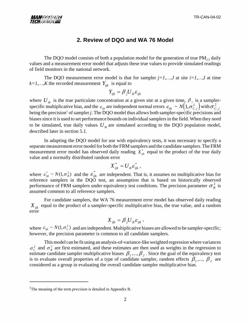
The DQO model consists of both a population model for the generation of true PM2.5 dailyvalues and a measurement error model that adjusts these true values to provide simulated readingsof field monitors in the national network.
The DQO measurement error model is that for sampler j=1,…,J at site i=1,…,I at timek=1,…,K the recorded measurement is equal toijkY
ijk j ik ijkY Uβ ε=where is the true particulate concentration at a given site at a given time, is a sampler-ikU jβspecific multiplicative bias, and the are independent normal errors withijkε ( )ε σijk C jN~ , ,1 2 2
,C jσbeing the precision1 of sampler j. The DQO model thus allows both sampler-specific precisions andbiases since it is used to set performance bounds on individual samplers in the field. When they needto be simulated, true daily values are simulated according to the DQO population model,ikUdescribed later in section 5.1.
In adapting the DQO model for use with equivalency tests, it was necessary to specify aseparate measurement error model for both the FRM samplers and the candidate samplers. The FRMmeasurement error model has observed daily reading equal to the product of the true daily*
ijkXvalue and a normally distributed random error
,* *ijk ik ijkX U ε=
where and the are independent. That is, it assumes no multiplicative bias for* 2~ (1, )ijk RNε σ *ijkε
reference samplers in the DQO test, an assumption that is based on historically observedperformance of FRM samplers under equivalency test conditions. The precision parameter is2
Rσassumed common to all reference samplers.
For candidate samplers, the WA 76 measurement error model has observed daily reading equal to the product of a sampler-specific multiplicative bias, the true value, and a randomijkX
error
,ijk j ik ijkX Uβ ε=where and are independent. Multiplicative biases are allowed to be sampler-specific;2~ (1, )ijk CNε σhowever, the precision parameter is common to all candidate samplers.
This model can be fit using an analysis-of-variance-like weighted regression where variances and are first estimated, and these estimates are then used as weights in the regression to2
Cσ 2Rσ
estimate candidate sampler multiplicative biases ,..., . Since the goal of the equivalency test1β Jβis to evaluate overall properties of a type of candidate sampler, random effects ,..., are1β Jβconsidered as a group in evaluating the overall candidate sampler multiplicative bias.

TR-CAN-04-02
3
The WA 76 report thus recommended an equivalency test where candidate samplers wereevaluated according to a DQO measurement error model. The report did not recommend theretention of an additive bias (intercept) or correlation from the current equivalency tests. As willnow be seen, trends in the field data suggest that these parameters might still be useful in anequivalency test.

TR-CAN-04-02
2All PM2.5 concentration data in this report are given in :g/m3.
4
3. Review of Field Samples
Field data were provided from five sites that had both FRM and continuous monitors present.These five sites—Bakersfield, Detroit, New York, Tampa, and Winston-Salem—were selected torepresent a broad spectrum of geographic regions, climatic regions, and continuous sampler types.Field data for each site consisted of time series of a single or a collocated pair of FRM samplers andof a single or a collocated pair of continuous samplers. Although some of these data should allowa basic evaluation of a proposed equivalency testing method, the data sets themselves were notcollected as equivalency tests. For equivalency tests, fewer days (currently a minimum of 10) andmore replicates (currently three) of both FRM and candidate samplers would be collected.
Of the sites, the Bakersfield site had both paired FRM and continuous samplers, while NewYork and Detroit had paired FRM and a single continuous. The Tampa site had a single FRM andtwo varieties of paired continuous samplers. The Winston-Salem site had only a single FRM anda single continuous. Thus, the Bakersfield site may be considered most representative of anequivalency test, having replicate samplers of both FRM and continuous kind.
Some exploratory data analysis for each of these sites is now presented. For each site,scatterplots of daily readings are given to illustrate association among the readings. Some time seriesare provided for interpretation of temporal trends.
3.1 Bakersfield Field DataThe Bakersfield samples provide the only data set with both collocated reference and
candidate samplers. These replications of both kinds of samplers make this data set most similar tocurrent equivalency tests.
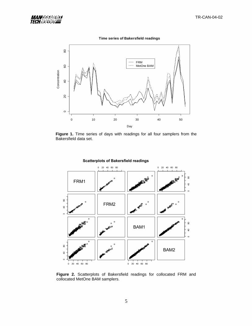
Time series plots2 of the Bakersfield readings are given in Figure 1. Trends illustrated by thisseries are that the continuous MetOne BAM samplers tend to produce higher readings than the FRMsamplers, and that samplers of the same type tend to have more similar readings than those ofdifferent types.
The consistency of readings within sampler types is further illustrated by the pair-wisescatterplots given in Figure 2. Paired readings within sampler types show relatively high correlationas compared to correlations across sampler types. There appear to be relatively few outliers, withthe apparent exception of a couple of smaller FRM readings.
TR-CAN-04-02
5
0 10 20 30 40 50
020
4060
80
Time series of Bakersfield readings
Day
Con
cent
ratio
nFRMMetOne BAM
Figure 1. Time series of days with readings for all four samplers from theBakersfield data set.
Figure 2. Scatterplots of Bakersfield readings for collocated FRM andcollocated MetOne BAM samplers.

TR-CAN-04-02
6
That the correlation between sampler types is less than might be expected, given thecorrelation within sampler types, is suggested by the correlation matrix of Table 1, where the across-type correlation is notably smaller than within type. Note that the average of the across-sampler-typecorrelations is 0.978, which exceeds the minimally required 0.97 of the current equivalency tests.The correlation of the sample means of the candidate and equivalent samplers equals 0.981, alsoexceeding the required amount.
Table 1. Sample Correlations among Bakersfield Samplers
FRM1 FRM2 BAM1 BAM2FRM1 1.000 0.993 0.978 0.980FRM2 0.993 1.000 0.974 0.981BAM1 0.978 0.974 1.000 0.994BAM2 0.980 0.981 0.994 1.000
Computing the regression statistics of the current equivalency tests gives an intercept of 5.89and a slope of 1.05. The slope satisfies the requirement that it lie between 0.95 and 1.05, but theintercept exceeds the bounds of -1 and 1. Thus, these field data for the collocated BAM samplersgive estimates that do not satisfy current equivalency requirements.
Similarly, the methods of WA 76 can be used to evaluate the Bakersfield data as if they werefrom an equivalency test. Table 2 gives precisions and biases for the Bakersfield data. Twoapproaches are taken, with and without outliers. The analysis without outliers removes twoobservations from the reference sampler data set: paired observations of (16.4, 8.5) and (1.0, 9.5).There did not appear to be any outliers in the candidate data. With outliers removed, both referenceand candidate samplers have estimated precisions better than the DQO-required 0.1. The averagemultiplicative bias of the two samplers is well above 1.1, so the candidate samplers would also failequivalency tests according to the DQO standards and WA 76 methods.
Table 2. Bakersfield Parameter Estimates for Candidate Samplers According to the WA 76 Model
Parameter Estimate with Outliers Estimate without OutliersReference precision 0.230 0.050Candidate precision 0.077 0.077Average candidate bias 1.350 1.350

TR-CAN-04-02
7
Figure 3. Scatterplots of Detroit readings for collocated FRM and an R&P TEOM runningat 50 °C.
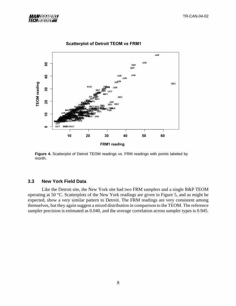
3.2 Detroit Field DataThe field data from Detroit were obtained from collocated FRM samplers and a continuous
R&P TEOM operating at 50 °C. Scatterplots of the Detroit readings are given in Figure 3 andsuggest that the FRM samplers show relatively good within-sampler precision (estimated referencesampler precision is 0.055); however, in comparison with the continuous TEOM sampler, thescatterplots suggest a bivariate mixed distribution. This mixed distribution appears to have twocomponent distributions, each associated with seasonal effects as illustrated by Figure 4, whichgives a scatterplot of the TEOM versus the first FRM sampler with the points labeled according tomonth of the year. Of the two component distributions of Figure 4, one appears to largely representwarmer months, while the other the cooler ones. This mixed distribution might be expected todecrease the correlation, and the average of the correlation coefficients of the two FRM-continuouspairings is 0.82, which is well below the current equivalency requirement of 0.97.
TR-CAN-04-02
8
Figure 4. Scatterplot of Detroit TEOM readings vs. FRM readings with points labeled bymonth.
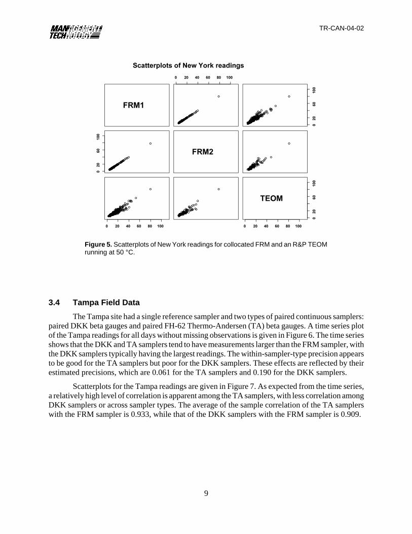
3.3 New York Field DataLike the Detroit site, the New York site had two FRM samplers and a single R&P TEOM
operating at 50 °C. Scatterplots of the New York readings are given in Figure 5, and as might beexpected, show a very similar pattern to Detroit. The FRM readings are very consistent amongthemselves, but they again suggest a mixed distribution in comparison to the TEOM. The referencesampler precision is estimated as 0.040, and the average correlation across sampler types is 0.945.
TR-CAN-04-02
9
Figure 5. Scatterplots of New York readings for collocated FRM and an R&P TEOMrunning at 50 °C.
3.4 Tampa Field DataThe Tampa site had a single reference sampler and two types of paired continuous samplers:
paired DKK beta gauges and paired FH-62 Thermo-Andersen (TA) beta gauges. A time series plotof the Tampa readings for all days without missing observations is given in Figure 6. The time seriesshows that the DKK and TA samplers tend to have measurements larger than the FRM sampler, withthe DKK samplers typically having the largest readings. The within-sampler-type precision appearsto be good for the TA samplers but poor for the DKK samplers. These effects are reflected by theirestimated precisions, which are 0.061 for the TA samplers and 0.190 for the DKK samplers.
Scatterplots for the Tampa readings are given in Figure 7. As expected from the time series,a relatively high level of correlation is apparent among the TA samplers, with less correlation amongDKK samplers or across sampler types. The average of the sample correlation of the TA samplerswith the FRM sampler is 0.933, while that of the DKK samplers with the FRM sampler is 0.909.

TR-CAN-04-02
10
0 5 10 15 20 25 30
010
2030
4050
Time series of Tampa readings
Day
Con
cent
ratio
n
FRMDKKTA
Figure 6. Time series of days with complete data for the Tampa site. Series arefederal reference method (FRM) samplers, DKK beta gauge samplers, and Thermo-Andersen (TA) beta gauges.
Figure 7. Scatterplots of Tampa readings for the FRM, the Thermo-Andersen,and the DKK beta gauges.
TR-CAN-04-02
11
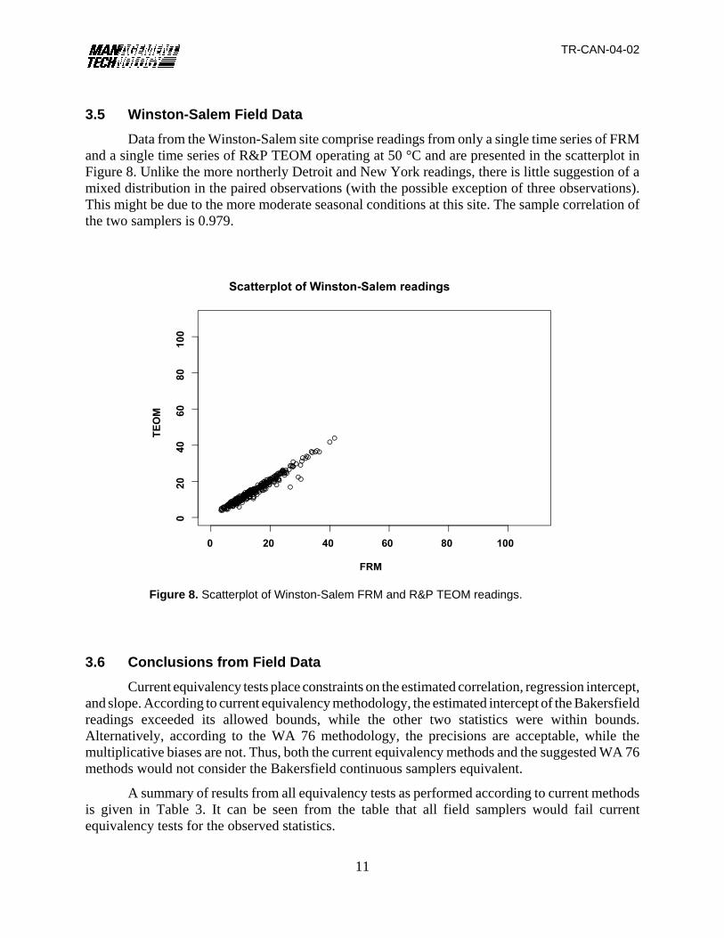
Figure 8. Scatterplot of Winston-Salem FRM and R&P TEOM readings.
3.5 Winston-Salem Field DataData from the Winston-Salem site comprise readings from only a single time series of FRM
and a single time series of R&P TEOM operating at 50 °C and are presented in the scatterplot inFigure 8. Unlike the more northerly Detroit and New York readings, there is little suggestion of amixed distribution in the paired observations (with the possible exception of three observations).This might be due to the more moderate seasonal conditions at this site. The sample correlation ofthe two samplers is 0.979.
3.6 Conclusions from Field DataCurrent equivalency tests place constraints on the estimated correlation, regression intercept,
and slope. According to current equivalency methodology, the estimated intercept of the Bakersfieldreadings exceeded its allowed bounds, while the other two statistics were within bounds.Alternatively, according to the WA 76 methodology, the precisions are acceptable, while themultiplicative biases are not. Thus, both the current equivalency methods and the suggested WA 76methods would not consider the Bakersfield continuous samplers equivalent.
A summary of results from all equivalency tests as performed according to current methodsis given in Table 3. It can be seen from the table that all field samplers would fail currentequivalency tests for the observed statistics.

TR-CAN-04-02
12
Table 3. Field Data Estimated Parameter Values Based on Current Equivalency Methods
SiteContinuous
Sampler Type
Number of Reference Samplers/Continuous Samplers/Days
Complete Observations α̂ β̂ ρ̂Bakersfield BAM 2/2/52 5.89 1.05 0.981Bakersfield1 BAM 2/2/50 5.55 1.06 0.982Detroit TEOM 2/1/31 0.36 0.70 0.826New York TEOM 2/1/111 1.86 0.92 0.945Tampa DKK 1/2/30 2.64 1.54 0.905Tampa TA 1/2/25 0.04 1.23 0.936
1After removal of two FRM sampler outliers as described in section 3.1.
The differences between the DQO/WA 76 and current equivalency methods are summarizedin Table 4, which gives the quantities measured as well as the required ranges by each approach. Theonly common parameter among them is the multiplicative bias.
Table 4. Comparison of Quantities Estimated between Current DQO and Equivalency Methods
Parameter DQO/WA 76 RequirementCurrent
Equivalency Tests RequirementPrecision Yes #0.1 No —Multiplicative bias (:g/m3) Yes $0.9 and #1.1 Yes $0.95 and #1.05Additive bias (:g/m3) No — Yes $-1 and #1Correlation of means No — Yes $0.97
After analysis of the field data, both the precision and the slope remain useful quantities tomeasure, as they still minimally describe the multiplicative error model, and the observed data (atleast for FRM samplers) appeared to be consistent with this basic measurement error model.
Although the WA 76 report did not recommend the inclusion of an additive bias parameter,the estimated non-zero intercept of the Bakersfield continuous samplers suggests that for somesamplers at some sites the addition of an intercept parameter might lead to a better fitting model.Including an intercept does not fundamentally change the measurement error model, as the currentDQO model is simply the zero intercept special case. The intercept is not currently part of the DQOmethodology, however, and so adding it to the equivalency tests suggests perhaps introducing it intothe DQO methodology as well.
The field data also suggest that correlation can be a useful parameter to estimate in anequivalency test. The Bakersfield readings suggested a somewhat lower across-sampler-type

TR-CAN-04-02
13
correlation than might be expected, based on the within-type correlations, and the readings fromDetroit and New York revealed a likely mixed distribution of measurement errors, where this mixeddistribution allowed low across-sampler-type correlations. Correlation thus might be retained in thetests as a check on model adequacy, as is now described.
The field data analyzed here suggest that the correlation, and potentially the intercept, allowan evaluation of DQO model adequacy within the equivalency tests. They test for model adequacyboth by generalizing the standard DQO model and by allowing for the detection of the influence ofadditional, unmeasured variables on sampler performance. To illustrate, consider the WA 76candidate sampler measurement error model in the presence of unmeasured variables , ,ikZ 1,...,i I=
that are added to the candidate sampler readings, so at a given site on a given day1,...,k K=
.ijk ik ijk ikX U Zβ ε= +These unmeasured variables might have any distribution (including mixed distributions such as seenin Detroit and New York), but suppose that they have independent normal distributions
. The model then corresponds to where and2~ (5, /100)ik ikZ N U *ijk ik ijk ikX U Zα β ε= + + 5α =
. Thus, a first effect of this variable is that its expectation can be absorbed into* 2~ (0, /100)ik ikZ N Uthe intercept, and the intercept therefore does necessarily represent an inherent property of acandidate sampler.
A scatterplot of simulated measurements for two reference and two candidate samplers inthe presence of this unmeasured variable model is given in Figure 9. From this figure, it can be seenthat the correlation across sampler types is less than within types, an effect which is due to thepresence of the unmeasured variables. This is a similar situation to that in Bakersfield, where suchvariables may have affected the correlation.
The data analysis then leads to the recommendation that parameters for additive bias,multiplicative bias, precision, and correlation be included in the equivalency tests. Precision andmultiplicative bias are the basic parameters of the sampler measurement error model, with theadditive bias allowing a somewhat more general model. In addition to correlation, additive bias canalso be used to assess the fit of the basic model, with lack of fit potentially due to the presence ofunmeasured variables or some other functional misspecification of the model.

TR-CAN-04-02
14
Figure 9. Scatterplots illustrating the effect of an unmeasured variable on thecorrelation.

TR-CAN-04-02
17
4. Proposed Measurement Error Model
The model for reference sampler measurement error of sampler j at time k at site i has referencesampler reading given as*
ijkX* *ijk ik ijkX U ε=
where is the true daily value and is the multiplicative measurement error. The errors areikU *ijkε
assumed independent and normally distributed with mean equal to 1 and precision* 2~ (1, )ijk RNε σ.Rσ
For the candidate samplers, the measurement error model is more general, with candidatesampler reading given asijkX
ijk ik ijkX Uα β ε= +where is an intercept allowing for additive bias, is a slope allowing for multiplicative bias,α βand the are independent errors that are normally distributed with mean 1 andijkε 2~ (1, )ijk CNε σprecision .Cσ

TR-CAN-04-02
19
215 10.238sin 1,...,1095365k
j kπμ ⎛ ⎞= + =⎜ ⎟⎝ ⎠
5. Performance Bounds for Model Parameters
Each equivalency test parameter must fall within some range of values that allows thecandidate sampler to exhibit equivalent performance. Current bounds based on DQO methodologyor equivalency tests have been given in Table 4. The parameters to be estimated and their boundsdiffer for the two methods of the table, and the recommendation of WA 76 was that future boundsbe based on the DQO methodology.
That bounds be based on DQO methods is again recommended in this report, and the DQOmethodology can be extended to provide bounds for the intercept in addition to the current slope andprecision. This extension is described in section 5.1.
A bound for correlation can be obtained as a function of the bounds for precision and ofparameters of the PM2.5 population process, which generates true daily means (in the DQOmethodology this would be the sine curve combined with the daily variation). Methods to obtainbounds for the correlation coefficient are given in section 5.2.
5.1 Bounds for the Precision, the Intercept, and the SlopeCurrent bounds for the precision and slope are determined by DQO grey-zone simulation.
This simulation is described in this section and is extended here to include an intercept. For specifiedpopulation mean, multiplicative bias, and precision, the current DQO simulations simulate manyrealizations of sampler three-year means to estimate an error rate equal to the proportion of timesthat the simulated three-year mean lies on the other side of 15.05 :g/m3 from the true simulationmean.
Each simulation run proceeds as follows:
1. Generate 3 × 365 = 1095 days of mean particulate readings according to the DQOsinusoidal population model of yearly mean 15.
2. Find the true daily particulate concentration for each day as where the kV k k kV eμ= keare independent lognormal errors of mean 1 and standard deviation 0.8. The three-yearrealized population mean is then ./1095k
kV V= ∑
3. Divide each year into four quarters and select 12 days at random from each quarteraccording to a 1 in 6 sampling scheme whose first day is the first day of the quarter.Only 12 days are selected per quarter to allow for 25% missing data. A total of n = 48× 3 = 144 days is selected from the 1095 available with labels given as .1 144,...,s s
4. Convert the realized process of mean into one with realized mean of interest V 0μ(e.g., , ) by dividing through by and multiplying by . The0 12.2μ = 0 18.8μ = V 0μadjusted true particulate concentrations for the DQO simulation days are then
TR-CAN-04-02
20
i is si
eZ
Vμ ε
=
/ii
Z Z n= ∑
0
1,...isiU i n
Vμ μ
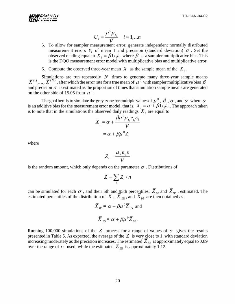
= =5. To allow for sampler measurement error, generate independent normally distributed
measurement errors of mean 1 and precision (standard deviation) . Set theiε σobserved reading equal to where is a sampler multiplicative bias. Thisi i iX Uβ ε= βis the DQO measurement error model with multiplicative bias and multiplicative error.
6. Compute the observed three-year mean as the sample mean of the .X iXSimulations are run repeatedly times to generate many three-year sample meansN
, after which the error rate for a true mean of with sampler multiplicative bias (1) ( ),..., NX X 0μ βand precision is estimated as the proportion of times that simulation sample means are generatedσon the other side of 15.05 from .0μ
The goal here is to simulate the grey-zone for multiple values of , , , and where 0μ β σ α αis an additive bias for the measurement error model, that is, . The approach takeni i iX Uα β ε= +is to note that in the simulations the observed daily readings are equal toiX
0
0
i is s ii
i
eX
VZ
βμ μ εα
α βμ
= +
= +
where
is the random amount, which only depends on the parameter . Distributions ofσ
can be simulated for each , and their 5th and 95th percentiles, and , estimated. Theσ .05Z .95Zestimated percentiles of the distribution of , , and are then obtained asX .05X 95X
and0.05 .05= X Zα βμ+
.0.95 .95= X Zα βμ+
Running 100,000 simulations of the process for a range of values of gives the resultsZ σpresented in Table 5. As expected, the average of the is very close to 1, with standard deviationZincreasing moderately as the precision increases. The estimated is approximately equal to 0.89.05Zover the range of used, while the estimated is approximately 1.12.σ .95Z

TR-CAN-04-02
21
Table 5. Sample Means, Standard Deviations, and 5th and 95th Percentiles forOne Million Simulations of at Varying Sampler PrecisionsZ
Precision( )σ
Sample Mean ofZ
Sample StandardDeviation of Z
Estimated
.05Z Estimated .95Z
0.05 1.000 0.070 0.890 1.1190.06 1.000 0.070 0.890 1.1190.07 1.000 0.070 0.890 1.1190.08 1.000 0.070 0.890 1.1190.09 1.000 0.070 0.890 1.1200.10 1.000 0.070 0.889 1.1200.11 1.000 0.071 0.889 1.1200.12 1.000 0.071 0.889 1.1210.13 1.000 0.071 0.888 1.1210.14 1.000 0.071 0.888 1.1220.15 1.000 0.072 0.887 1.1220.20 1.000 0.073 0.885 1.125
Thus, it appears that the percentiles can be approximated as0
.05 = 0.89X α βμ+and
0.95 = 1.12X α βμ+
over all of interest. For example, using the current DQO lower bound , ,σ 0 12.2μ = 0α =, then1.1β =
,.95 = 1.12(1.1)(12.2) 15.03X =and if using the current DQO upper bound , , , then0 18.8μ = 0α = 0.9β =
..05 = 0.89(0.9)(18.8) 15.06X =The results given in Table 5 suggest that precision is not very important as far as three-year
average attainment decisions are concerned. Its bounds might be set for reasons other than DQOattainment. Currently the bound is 0.10, although it could rise to 0.15 or even 0.20 with little effecton the grey zone.
Given that precision might largely be ignored, the results of Table 5 also suggest allowableranges for and when considered jointly. For a fixed grey-zone boundary and fixed percentileα βvalue (15.05), we can solve for in terms of (or vice versa), for example,α β
0.05= -0.89 15.05 0.89 18.8 15.05 16.73Xα βμ β β= − = −
.0.95= -1.12 15.05 1.12 12.2 15.05 13.66Xα βμ β β= − = −
TR-CAN-04-02
22
0.90 0.95 1.00 1.05 1.10
-4-2
02
4
Allowable multiplicative and additive bias
Beta
Alp
ha
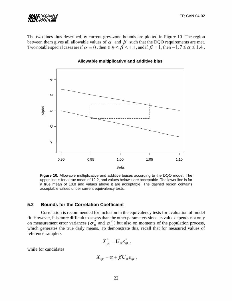
Figure 10. Allowable multiplicative and additive biases according to the DQO model. Theupper line is for a true mean of 12.2, and values below it are acceptable. The lower line is fora true mean of 18.8 and values above it are acceptable. The dashed region containsacceptable values under current equivalency tests.
The two lines thus described by current grey-zone bounds are plotted in Figure 10. The regionbetween them gives all allowable values of and such that the DQO requirements are met.α βTwo notable special cases are if , then , and if , then .0α = 0.9 1.1β≤ ≤ 1β = 1.7 1.4α− ≤ ≤
5.2 Bounds for the Correlation CoefficientCorrelation is recommended for inclusion in the equivalency tests for evaluation of model
fit. However, it is more difficult to assess than the other parameters since its value depends not onlyon measurement error variances ( and ) but also on moments of the population process,2
Rσ 2Cσ
which generates the true daily means. To demonstrate this, recall that for measured values ofreference samplers
,* *ijk ik ijkX U ε=
while for candidates
.ijk ik ijkX Uα β ε= +

TR-CAN-04-02
23
* *
*
* *
2 * *
2 2
2
[ , ] [ , ]
[ , ]
( [ ] [ ] [ ])
( [ ] [ ] [ ] [ ] [ ] [ ] [ ])
( [ ] [ ] )
i
U
Cov X X Cov U U
Cov U U
E U U E U E U
E U E E E U E E U E
E U E U
ε α β ε
β ε ε
β ε ε ε ε
β ε ε ε ε
β
βσ
= +
=
= −
= −
= −
=
* *
2 * 2 * *
2 * 2 2
2 2 2
2 2 2
[ ] [ ]
[ ( ) ] [ ] [ ]
[ ] [( ) ] [ ]
[ ]( 1) [ ]
[ ]R
U R
Var X Var U
E U E U E U
E U E E U
E U E U
E U
ε
ε ε ε
ε
σ
σ σ
=
= −
= −
= + −
= +
2 2 2 2
[ ] [ ]( [ ])U C
Var X Var UE U
α β ε
β σ σ
= +
= +
( )( ) ( )( )
**
*
2
2 2 2 2 2 2 2
122 2 2 2
[ , ][ , ][ ] [ ]
( [ ]) ( [ ])
1 1 1 1
U
U R U C
R U C U
Cov X XCorr X XVar X Var X
E U E Uβσ
σ σ β σ σ
σ τ σ τ−
− −
=
=+ +
⎡ ⎤= + + + +⎣ ⎦
Dropping indices for clarity (and since is now drawn randomly according to the sampling schemeUand population process), consider a pair of reference and candidate measurements collected*,X Xon the same day at the same site, with true value and errors , respectively. The covarianceU * ,ε εof paired reference and candidate measurements is then
and the variance of the reference measurements equals
and similarly the variance of the candidate measurements equals
so that the correlation of reference and candidate measurements equals
where is the population coefficient of variation, the ratio of the population standard deviationUτto the population mean
.U
UU
στμ
=
Thus, the correlation only depends on , and population process parameter , and does not2Cσ 2
Rσ Uτdepend on either or .α β
TR-CAN-04-02
24
( ) ( )1
22 2* 2 2
*[ , ] 1 1 1 1CRU UCorr X X
J Jσσ τ τ
−
− −⎡ ⎤⎛ ⎞⎛ ⎞= + + + +⎢ ⎥⎜ ⎟⎜ ⎟
⎝ ⎠⎝ ⎠⎣ ⎦
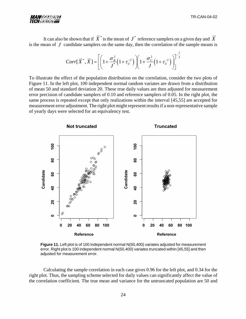
Figure 11. Left plot is of 100 independent normal N(50,400) variates adjusted for measurementerror. Right plot is 100 independent normal N(50,400) variates truncated within [45,55] and thenadjusted for measurement error.
It can also be shown that if is the mean of reference samplers on a given day and *X *J Xis the mean of candidate samplers on the same day, then the correlation of the sample means isJ
To illustrate the effect of the population distribution on the correlation, consider the two plots ofFigure 11. In the left plot, 100 independent normal random variates are drawn from a distributionof mean 50 and standard deviation 20. These true daily values are then adjusted for measurementerror precision of candidate samplers of 0.10 and reference samplers of 0.05. In the right plot, thesame process is repeated except that only realizations within the interval [45,55] are accepted formeasurement error adjustment. The right plot might represent results if a non-representative sampleof yearly days were selected for an equivalency test.
Calculating the sample correlation in each case gives 0.96 for the left plot, and 0.34 for theright plot. Thus, the sampling scheme selected for daily values can significantly affect the value ofthe correlation coefficient. The true mean and variance for the untruncated population are 50 and

TR-CAN-04-02
25
400, while for the truncated population they are 50 and 8.23. Assuming reference sampler precisionof 0.05 and candidate sampler precision of 0.10, the theoretical values of the correlation for eachpopulation are therefore 0.96 and 0.38, respectively, based on population values for ofUτ
and .400 / 50 0.4= 8.23 / 50 0.057=
Theoretical correlations for various combinations of the population precision-mean ratio Uτand the candidate precision are provided in Table 6. From the table, it can be seen that providedCσ
is about 0.5 or greater the correlation should be 0.97 or greater for candidate sampler precisionUτof 0.10 or less. Correlation increases rapidly as the precision becomes large relative to the mean.
Table 6. Correlations for Single Reference vs. Candidate Samplers for Various and .Uτ CσReference sampler precision is set equal to 0.05.
Uτ Cσ0.05 0.06 0.07 0.08 0.09 0.10 0.11 0.12 0.13 0.14 0.15 0.20
0.01 0.04 0.03 0.03 0.02 0.02 0.02 0.02 0.02 0.02 0.01 0.01 0.010.02 0.14 0.12 0.10 0.09 0.08 0.07 0.07 0.06 0.06 0.05 0.05 0.040.04 0.39 0.35 0.31 0.28 0.25 0.23 0.21 0.20 0.18 0.17 0.16 0.120.10 0.80 0.77 0.73 0.70 0.66 0.63 0.60 0.57 0.54 0.52 0.49 0.400.20 0.94 0.93 0.91 0.90 0.88 0.86 0.85 0.83 0.81 0.79 0.77 0.680.25 0.96 0.95 0.94 0.93 0.92 0.91 0.89 0.88 0.86 0.85 0.83 0.760.33 0.98 0.97 0.96 0.96 0.95 0.94 0.93 0.92 0.91 0.90 0.89 0.830.50 0.99 0.98 0.98 0.98 0.97 0.97 0.97 0.96 0.95 0.95 0.94 0.911.00 1.00 0.99 0.99 0.99 0.99 0.99 0.99 0.98 0.98 0.98 0.98 0.962.00 1.00 1.00 1.00 0.99 0.99 0.99 0.99 0.99 0.99 0.99 0.98 0.97
Table 7 provides correlations calculated in the same way as Table 6 except that they arebased on averages of three reference samplers versus three candidate samplers. Similar trends areapparent as in Table 6, although the correlations are somewhat higher due to the decrease in thevariance of the sample means.
Table 7. Correlations for Sample Means of Three Reference vs. Three Candidate Samplers for Various and . Reference sampler precision is set equal to 0.05.Uτ Cσ
Uτ Cσ0.05 0.06 0.07 0.08 0.09 0.10 0.11 0.12 0.13 0.14 0.15 0.20
0.01 0.11 0.09 0.08 0.07 0.06 0.06 0.05 0.05 0.04 0.04 0.04 0.030.02 0.32 0.28 0.25 0.23 0.20 0.19 0.17 0.16 0.15 0.14 0.13 0.100.04 0.66 0.61 0.57 0.53 0.49 0.46 0.43 0.41 0.38 0.36 0.34 0.270.10 0.92 0.91 0.89 0.87 0.85 0.83 0.81 0.79 0.77 0.75 0.72 0.630.25 0.99 0.98 0.98 0.98 0.97 0.97 0.96 0.95 0.95 0.94 0.94 0.900.33 0.99 0.99 0.99 0.99 0.98 0.98 0.98 0.97 0.97 0.96 0.96 0.940.50 1.00 0.99 0.99 0.99 0.99 0.99 0.99 0.99 0.98 0.98 0.98 0.971.00 1.00 1.00 1.00 1.00 1.00 1.00 1.00 0.99 0.99 0.99 0.99 0.992.00 1.00 1.00 1.00 1.00 1.00 1.00 1.00 1.00 1.00 1.00 0.99 0.99

TR-CAN-04-02
26
The results of this section show that the correlation between reference and candidatesamplers expected if the measurement error models are true depends on both the moments of thepopulation process that generates the true daily values and the precisions of each type of sampler.Methods to estimate the correlation expected if the model were true and also the sample correlationare given later in section 6.3.

TR-CAN-04-02
27
6. Parameter Estimation
Methods to estimate the parameters of interest in an equivalency test are now provided. Notethat, due to resource limitations in completion of this work, it has not been possible to investigatestatistical issues relating to sampling error, such as interval estimation or hypothesis tests.
6.1 Maximum Likelihood EstimationThe measurement error model of section 4 can be fit numerically according to the maximum
likelihood approach. Once the model has been specified, the natural logarithm of the correspondinglikelihood function can be maximized numerically to obtain maximum likelihood estimates for theparameters of interest.
For the model considered here the likelihood is a product of (IJK)2 normal densities basedon the assumptions that the are independent and normally distributed , and the*
ijkX 2 2( , )ik ik RN U U σare independent and normally distributed as .ijkX 2 2 2( , )ik ik RN U Uα β β σ+
The challenge in using likelihood methods for this problem is that the number of parametersto be estimated is not only the four of , , , and , but also the IK parameters for each ofα β Cσ Rσthe true daily PM2.5 values . The dimension of the parameter space over which maximizationikUmust be done can therefore be very large, increasing with both days and sites. These additionalparameters are known statistically as nuisance parameters and can either be numerically integratedout of the likelihood or maximized in addition to the parameters of interest. The approach taken herewill be to maximize the full model, and, remarkably, the optimization procedures used converge forall data sets considered here, up to 111 days of observations (a 115-dimensional space). Incomparison, a standard equivalency test should have between 30 and 45 days of observations.
Starting values for the maximization are taken as the day means for the reference samplers,an intercept of zero, a slope of 1, reference precision of 0.05, and candidate precision 0α̂ 0β̂ 0ˆ Rσ 0ˆCσof 0.10. Code for performing the maximization in the R computing language is provided inAppendix A.
6.2 Other EstimatorsIn addition to maximum likelihood estimation of model parameters, the precisions of both
reference and candidate samplers can be estimated using simple estimators. These estimators areuseful in that they guard against situations where the model is misspecified, possibly with additionalsources of error present such as unmeasured variables (as described in section 3.6). They do this byrelying only on the candidate or reference data, depending on which precision is being measured.This is more important for candidate samplers than for reference samplers, as the reference samplermodel is well supported by historical data and so the likelihood estimate (particularly if restrictedto reference data alone) should be reasonable.
TR-CAN-04-02
28
( ) log( ) ( 1)ikijk ik ijk
ik
Uh UU
βε α β εα β
≈ + + −+
2
22
[ ( )] [ ]
1
1
ikik ijk ijk
ik
ik
UVar h VarU
U
βε εα β
σαβ
⎛ ⎞≈ ⎜ ⎟+⎝ ⎠
=⎛ ⎞+⎜ ⎟
⎝ ⎠
In general, the model considered here is of an additive intercept with multiplicative error:
ijk ik ijkX Uα β ε= +where the are independent errors that might be assumed to be normally distributedijkε
with mean 1 and precision . The goal is to develop a simple estimator for ,2~ (1, )ijk CNε σ Cσ Cσwhich is difficult here since applying a log transform does not in this case make the model additivedue to the additive intercept.
The approach taken here will be to note that it is expected that the squares of both precisionswill be well less than 1, i.e., and , and for random2 20.05 .0025 1Rσ ≤ = < 2 20.2 .04 1Cσ ≤ = <variable with and small, the Taylor expansion of function around ε [ ] 1E ε = 2[ ]Var ε σ= ( )h ε [ ]E εis approximately
( ) ( [ ]) '( [ ])( [ ])h h E h E Eε ε ε ε ε≈ + −where is the first derivative of , assuming it exists. If , then the'h h ( ) log( )ijk ik ijkh Uε α β ε= +expansion can be written
and so
This result has two consequences:
1. For reference samplers, and so 0α ≡
.2[ ( )]ik ijkVar h ε σ≈ Thus, the sample variance of the log-transformed reference sampler measurements
at a given site on a given day is a closely approximating estimator of . That is,2Rσ
2 21R k
kS
IKσ = ∑%
where is the sample variance of the log reference sampler measurements2kS
at site i at time k. The precision estimator is then .*log( )ijkX 2R Rσ σ=% %

TR-CAN-04-02
29
ikUα
β
ikUα
β
2 21C k
k
SIK
σ = ∑%
2C Cσ σ=% %
2. For candidate samplers, in general and so0α ≠
is also nonzero. However, as gets large,ikU
becomes small and so the approximation is closer for days with larger averagereadings. So an estimator might be
where is the sample variance of the log candidate sampler measurements at site i at2kS log( )ijkX
time k restricted to days with larger reference sampler readings, perhaps over 20. The candidatesampler precision is then estimated as
.
An alternative approach might use substitution of and from the likelihood estimation,α βalthough that is not studied here. Note that, provided is not too far from zero, the estimatorαshould be reasonably good and some idea as to what value takes can be obtained from theαlikelihood estimation.
6.3 Correlation and Its EstimationIn addition to estimating parameters of the measurement error model, we are also interested
in estimating the correlation between candidate and reference samplers and comparing the estimatedvalue to a correlation expected if the model were true. As described previously, the estimatedcorrelation coefficient can provide a measure of model fit.
The correlation between reference and candidate samplers can be estimated with data froman equivalency test; however, it is difficult to interpret without knowing what value might beexpected were the model correct. This expected value can, however, be estimated if a consistentestimator of , the coefficient of variation at site i, can be obtained. It turns out that the reference,U iτsampler data allow such an estimator.
Using the approach in section 5.2, it can be shown that for collocated reference samplers j,jN
* * 2, ' '[ , ] 'i jj ijk ij k UCov X X j jσ= ≠
and so the sample covariance among reference samplers is an estimate of the population processvariance. Since the population process mean at site i can be estimated as the sample mean of,U iμ

TR-CAN-04-02
30
2,
,,
* *,
*
ˆˆ
ˆ
2 ˆ ( , )( 1)
1
U iU i
U i
i mn imk inkm n m
ijkjk
Cov x xJ J
xJK
στ
μ
≠
=
−=
∑∑
∑
( ) ( )1
2 2 2,0 ,02 2
0, , ,*ˆ ˆ ˆ1 1 1 1R C
i U i U iJ Jσ σ
ρ τ τ−
− −⎡ ⎤⎛ ⎞⎛ ⎞
= + + + +⎢ ⎥⎜ ⎟⎜ ⎟⎜ ⎟⎜ ⎟⎢ ⎥⎝ ⎠⎝ ⎠⎣ ⎦
the reference sampler values at that site, the population coefficient of variation at site i can thereforebe estimated as
where is the sample covariance between reference samplers m and n at site i.* *,
ˆ [ , ]i mn imk inkCov x xThus, the population coefficient of variation at a given site is estimated as the square root of theaverage of sample covariances among all pairings of reference samplers at the site divided by thesample mean of the reference sampler readings at that site. Using this estimated coefficient ofvariation, a target correlation for the means of reference and candidate samplers at the site is0,ˆ iρthen estimated as
where and are the number of reference and candidate samplers at the site. In estimating this*J Jtarget correlation, values for and can be obtained either as sample estimates or as the,0Rσ ,0Cσlargest allowable values, for example, and . If sample estimates are used, it0.05Rσ = ,0 0.10Cσ =is recommended that variance estimates based on Taylor approximations, and not on maximumlikelihood, be used, since the Taylor approximation estimates are not affected by the types ofunmeasured variables described earlier.
To illustrate the method, suppose that 10 days of observations were available for twocollocated reference samplers and a candidate sampler for the first, non-truncated population ofFigure 11. For this simulated sample given in Table 8, the sample mean among paired referencesamplers is 33.5. The sample covariance among reference samplers is 433.4, and the estimated Uτis therefore 0.62. The target correlation is then found to be 0.980, assuming precisions of 0.05 forreference and 0.10 for candidate samplers. The sample correlation of the mean of the referencemeasurements versus the candidate measurements is 0.977.

TR-CAN-04-02
31
Table 8. Sample Data for Correlation Analysis
Day FRM1 FRM2 Candidate1 50.6 52.2 53.52 14.6 15.3 16.43 41.8 42.3 48.94 46.3 41.2 45.55 38.4 34.6 33.76 31.2 29.4 29.67 08.5 07.0 07.38 68.1 77.0 64.09 03.8 03.7 03.810 34.2 28.8 38.3

TR-CAN-04-02
33
20 40 60 80
020
4060
8010
0
True daily value
Sam
pler
read
ing
Figure 12. Simulated sampler readings vs. true daily values for referencesamplers (circles) and candidate samplers (triangles).
7. Illustration Using Simulated and Field Data Sets
This section applies the methods of this report to evaluate the performance of reference andcandidate samplers for both simulated and field data sets.
7.1 Model Fit Using Simulated DataA simulated data set was generated according to the design of the proposed equivalency
tests. For a single site, three reference and three candidate samplers had measurements simulatedfor 30 days. These measurements were simulated according to the measurement error model ofsection 4, with sampler parameter values set as , , , and . True1α = 0.95β = 0.05Rσ = 0.10Cσ =daily values (the ) were generated independently from a normal distribution of mean 50 and1kUstandard deviation of 25, with any negative values discarded until a total of 30 true daily values wereobtained. Figure 12 plots the simulated values for reference and candidate samplers against the truedaily values.

TR-CAN-04-02
34
20 40 60 80
2040
6080
True daily value
Est
imat
ed d
aily
val
ue
Figure 13. Estimated daily values vs. true daily values. A line of slope 1 throughthe origin is included for reference.
Fitting the model using the likelihood method gives maximum likelihood estimates of, , , and . Figure 13 plots the estimated daily valuesˆ 0.598α = ˆ 0.955β = ˆ 0.052Rσ = ˆ 0.097Cσ =
against the true daily values. This plot shows estimated mean daily values lying close to a 45-degreeline through the origin, as expected.
For comparison, the model was also fit using only the reference sampler data. In this case,the reference sampler precision is estimated as , close to its estimate under the full modelˆ 0.049Rσ =using both reference and candidate sampler data.
Using the Taylor approximation estimators and of section 6.3, estimates areRσ% Cσ% and over all days, or if restricting to days with reference0.059Rσ =% 0.095Cσ =% 0.097Cσ =%
means greater than 20. Note that, although these estimates are close to the true values, the likelihoodestimates would be preferred in this case as the measurement error model is known to hold exactlyfor the simulated data.

TR-CAN-04-02
35
For correlation, the population coefficient of variation for the 30 observed days is 0.41τ =and the estimated population coefficient of variation (using only the reference samplermeasurements) is . The target correlation of sample means can then be estimated as either ˆ 0.40τ = 0ˆ 0.985ρ =(using the largest allowable and ), using the estimated2
,0 0.05Rσ = 2,0 0.10Cσ = 0ˆ 0.986ρ =
precisions from the likelihood model, or using the estimated precisions based on Taylor0ˆ 0.985ρ =approximation. The sample correlation of the day means of the reference sampler measurementsversus the day means of the candidate sampler measurements is .ˆ 0.988ρ =
7.2 Model Fit Using Field DataTo evaluate the method’s performance with real data, the estimators described here were
applied to the field data of Bakersfield, Detroit, New York, and Tampa. The resulting estimates aregiven in Table 9.
The likelihood method was applied to obtain estimates of , , , and . It was alsoα β Cσ Rσapplied to the reference sampler data to obtain an estimate of based only on that data. Doing soRσprovides some insight into the effect of the assumed model structure on the estimate when candidatesampler data are included.
Taylor approximation estimates are obtained for and , with two sets of estimatesCσ Rσobtained for : the first based on the full candidate sampler data, as would be appropriate if it wasCσthought reasonable to assume that (perhaps supported by a hypothesis test or confidence0α =interval), and the second after truncating the candidate data above a somewhat arbitrary threshold.This second estimate reduces the effect of a non-zero on the estimate.α
Average sample correlations of reference and candidate samplers are obtained and comparedto expected values as computed using reference sampler data. These expected values are computedafter first estimating and then obtaining values for and . Values for precision areUτ Cσ Rσspecified either as fixed target values ( and ) or as Taylor approximation0.05Rσ = 0.10Cσ =estimates and , which are preferred over the maximum likelihood estimates as they areRσ% Cσ%more robust to model misspecification.
Not all statistics could be estimated for all sites since there are fewer replicate samplers thanwould be expected in an equivalency test. Sites with only one reference sampler do not allowestimation of or computation of the Taylor variance or of the maximum likelihood estimate Uτ Rσ% ˆ Rσbased only on the reference data. Sites with only one candidate sampler do not allow computationof the Taylor estimator , and consequently no estimate of a target correlation based onCσ% 0ρ̂estimated precisions. Current plans for equivalency tests call for three replicate candidate andreference samplers at each site, so all statistics could be computed for the resulting data set, ifneeded.
36
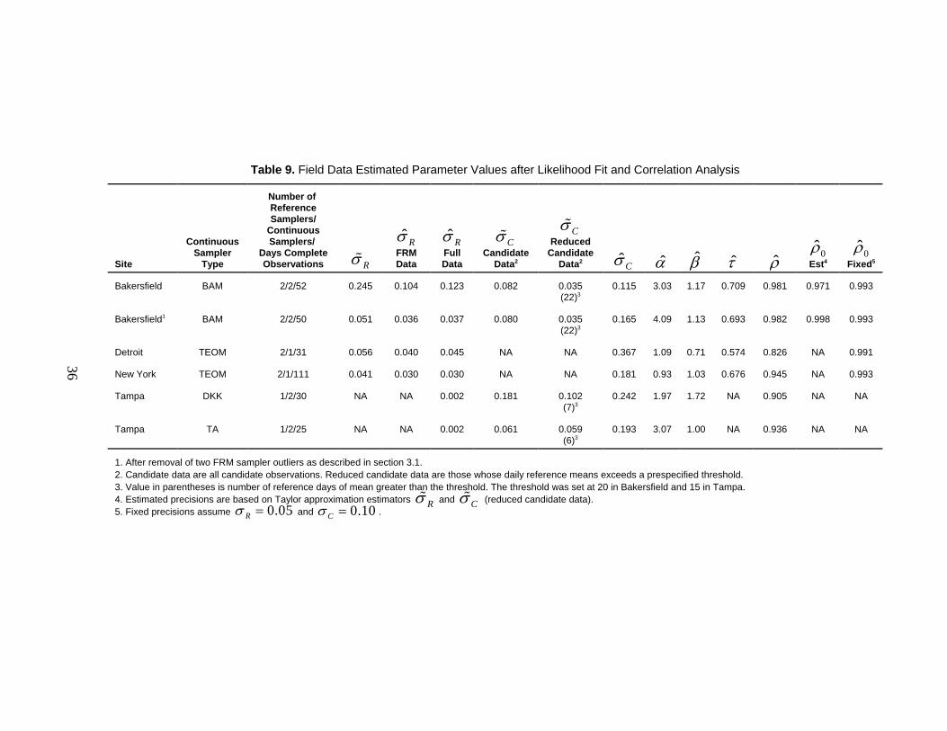
Table 9. Field Data Estimated Parameter Values after Likelihood Fit and Correlation Analysis
Site
ContinuousSampler
Type
Number of ReferenceSamplers/
ContinuousSamplers/
Days CompleteObservations Rσ%
ˆ RσFRMData
ˆ RσFullData
Cσ%Candidate
Data2
Cσ%Reduced
CandidateData2 ˆCσ α̂ β̂ τ̂ ρ̂
0ρ̂Est4
0ρ̂Fixed5
Bakersfield BAM 2/2/52 0.245 0.104 0.123 0.082 0.035(22)3
0.115 3.03 1.17 0.709 0.981 0.971 0.993
Bakersfield1 BAM 2/2/50 0.051 0.036 0.037 0.080 0.035(22)3
0.165 4.09 1.13 0.693 0.982 0.998 0.993
Detroit TEOM 2/1/31 0.056 0.040 0.045 NA NA 0.367 1.09 0.71 0.574 0.826 NA 0.991
New York TEOM 2/1/111 0.041 0.030 0.030 NA NA 0.181 0.93 1.03 0.676 0.945 NA 0.993
Tampa DKK 1/2/30 NA NA 0.002 0.181 0.102(7)3
0.242 1.97 1.72 NA 0.905 NA NA
Tampa TA 1/2/25 NA NA 0.002 0.061 0.059(6)3
0.193 3.07 1.00 NA 0.936 NA NA
1. After removal of two FRM sampler outliers as described in section 3.1. 2. Candidate data are all candidate observations. Reduced candidate data are those whose daily reference means exceeds a prespecified threshold.3. Value in parentheses is number of reference days of mean greater than the threshold. The threshold was set at 20 in Bakersfield and 15 in Tampa.4. Estimated precisions are based on Taylor approximation estimators and (reduced candidate data). Rσ% Cσ%5. Fixed precisions assume and .0.05Rσ = 0.10Cσ =

TR-CAN-04-02
37
The Bakersfield data set was fit twice, once for all days with complete data (both referenceand continuous samplers) and once for a reduced data set that had two apparent FRM outliersremoved. Removal of the outliers had the effect of strongly reducing the estimated reference methodprecision and increasing the target correlation based on estimated precisions. The data thus illustratethe importance of carefully checking for the presence of outliers.
Regarding the estimates of reference sampler precision by both Taylor approximation andmaximum likelihood, the estimates are largely consistent with exception of the Bakersfield data withoutliers present and the Tampa TA data. The Tampa TA data provide a maximum likelihoodestimate of based on only a single reference sampler and the full data set. This mightˆ 0.002Rσ =be a special case where the likelihood favors making the reference samplers extremely preciserelative to the candidate data whose variation is more directly measured. For the remaining sites,Taylor and likelihood estimates are similar, with the likelihood being somewhat smaller.
The candidate sampler precision estimates were uniformly larger than those for referencesamplers at each site. Furthermore, likelihood estimates tended to be larger than Taylor estimates.That the likelihood estimates are larger might be due to model misspecification, as the modelrequires that all variation present in the data be absorbed into its parameter estimates. This is goodif the model is believed (as it is in the DQO methodology); however, for departures from the model(due, for example, to outside sources of variation such as seasonality), the Taylor estimates mayprovide a more accurate representation of the precision of candidate measurements at a given siteon a given day. The improved precision is due to the Taylor estimates being based solely on thecandidate data.
However, Taylor estimates based on the full candidate data were typically larger than thosebased on the reduced data. This is the opposite of what was expected given the Taylor expansion ofsection 6.2 (leaving smaller values in should lead to smaller variance estimates). Further analysis(not shown) reveals larger variances of daily log observations for days of small reference samplermeans. This suggests an even more general reference and candidate sampler measurement errormodel than the one given here, namely, one that has both an additive and multiplicative error.Allowing for such a model might be seen as a topic for future work. Regardless, based on thisobserved effect, we are currently left without a good estimator for candidate precision for use withthe correlation tests. The likelihood estimator may be too large due to model misspecification, andthe Taylor estimate makes too few model assumptions. Based on the limited field data, it wouldseem that the full Taylor estimator might be preferred for use with correlation; however, lackingsolid justification for its use will suggest using fixed precision values.
Estimates of slope and intercept at all sites reveal that most have candidate slope-interceptcombinations that lie outside of ranges given in section 5.1. An exception would be the New Yorkdata set.
Sample correlation estimates between day means of reference and candidate samplers werefound to lie between 0.826 and 0.981, while population coefficient of variations were estimatedbetween 0.574 and 0.709. The estimated target correlations were all over 0.99 if fixed sampler andreference precisions were used. Excluding outliers from the Bakersfield data and using Taylorprecision estimates gave a target correlation of 0.998. Both Detroit and New York show correlationswell below their targets, while Bakersfield is somewhat close.
TR-CAN-04-02
39
8. Discussion
This report has analyzed field data for sites with both continuous and reference samplers toevaluate and suggest modifications to the DQO/WA 76 methodology for equivalency testing. Therecommendation of the report is that additive bias, multiplicative bias, precision, and correlationeach be included in the testing methods. Two steps in developing tests have been given:(1) estimators have been provided for each of these parameters, and (2) methods have been givento determine what ranges the parameters they estimate should fall in to consider a candidate samplerequivalent.
The completion of these two steps allows the development of equivalency tests similar inapproach to those currently used. The current tests have an experimental design (three samplers ofeach kind, minimum of 10 days, etc.) and statistics that are computed based on the observed datafor comparison to prespecified values. If these statistics fall within allowable bounds, then thesampler is equivalent. In a similar fashion, this report recommends statistics for use in a test andprovides methods to determine what values the statistics should take for large samples. Undercurrent proposed methods, these values are directly compared to sample statistics to perform the test.
Although not part of the current equivalency methods, some additional steps could befollowed to statistically complete the methodology. These would be either to simulate or find testdistributions for hypotheses of interest or to obtain interval estimates for parameters considered here.Interval estimates would be compared to allowable ranges of values to check if overlap existed.Given hypothesis tests or interval estimators, sample sizes for adequately powerful tests might beobtained.
Four parameters are recommended for equivalency testing: candidate sampler precision,candidate sampler additive bias (intercept), candidate sampler multiplicative bias (slope), andcorrelation of reference sampler and candidate sampler day means. It is recommended that the firstthree of these be estimated according to maximum likelihood and the correlation be estimated as itis currently.
Maximum likelihood methods offer the advantage that they more closely model the assumederror structure in the data. As described in WA 76, the implied model for the current equivalencytests least-squares fit is simple linear regression, which assumes that predictors are measuredwithout error—an assumption that does not hold for these data since there is error in the referencemeasurements. Having error in the predictors for a regression leads to biased parameter estimatorswith the slope being “attenuated” to be flatter than it should be and the intercept estimate biasedaccordingly. This may be problematic for the estimate of the intercept, since it is estimated as avalue along the regression line lying outside the range of the data. It is also required to lie within arelatively tight range, as seen in section 5.1. The other assumption of simple linear regression, whichdoes not hold here, is that the errors are of constant variance along the length of the regression curve.The main effect of this difference is that various tests and interval estimates based on simple linearregression assumptions are not appropriate.
TR-CAN-04-02
40
Likelihood methods also allow for future extensions to the methods to obtain intervalestimates and hypothesis tests. This can be done according to well-established theory.
The primary disadvantage of likelihood methods is that they are somewhat more complicatedto implement and require greater sophistication on the part of the modeler. Code is provided in theappendix that should allow their estimates to be obtained, and this should be evaluated for ease ofuse.
Each of the four tested parameters is now discussed in turn, with general recommendationsfor their incorporation into the equivalency test design.
The additive bias or intercept parameter was introduced into the measurement error modeldue to evidence of a non-zero intercept in the Bakersfield data. It is tested in current equivalencytests using the simple linear regression approach. As was shown in section 3.6, it can represent eithera property of the sampler or a property of the particular site, so equivalency tests at multiple sitesshould be required to determine if estimated intercepts are site-specific or not. The recommendedapproach to its estimation is the maximum likelihood approach. Like the slope, the precision of itsestimate improves with daily measurements that are well dispersed.
The multiplicative bias or slope parameter currently exists in both current equivalencymethods and the DQO methods. Like the intercept, it can be estimated using the maximumlikelihood approach. Also like the intercept, the estimate benefits from having reference and samplemeasurements that are well dispersed.
The precision parameter describes the variation in sampler measurement error. It can beestimated according to either maximum likelihood or Taylor approximation, with the likelihoodapproach being preferred. Neither of the estimators is entirely satisfactory, however, as the assumedmodel has been shown to not hold exactly (section 7.2), with errors being not strictly multiplicative.With that said, the resulting estimates should be close enough and make similar assumptions tocurrent methods used to estimate precision with field data. Furthermore, precision is the leastimportant of the parameters as far as DQO equivalency is concerned, and for moderate values it haslittle effect on the grey zone (section 5.1). As the Bakersfield data illustrated, its estimation issensitive to outliers, so care must be taken to identify and remove those from the final data.
The recommendation here is to estimate the correlation following the current approach—thatis, as the correlation of reference and candidate day means. This report has shown how its targetvalue for a given sample can be estimated (section 5.2), and this target depends on the reference andcandidate sampler precisions as well as the coefficient of variation of the underlying populationPM2.5 process. In estimating the target value, there is a choice of whether to substitute fixed worst-case precisions or to use the precision sample estimates. Both approaches were evaluated using thefield data, where for the estimated population coefficient of variations, all led to target correlationsof .99 or more (discarding outliers). The estimated target might then be adjusted in an ad hoc manner(say, by subtracting 0.01 or 0.02) to allow for some sampling error. Further study could providemore rigorous methods.

TR-CAN-04-02
41
9. References
U.S. EPA. 2002. DQO Companion, Version 1.0 Users’s Guide. EPA Work Assignment 5-07.
U.S. EPA. 2003. Data Quality Objectives for PM Continuous Methods, TR-4423-03-08. ResearchTriangle Park, NC: ManTech Environmental Technology, Inc.
TR-CAN-04-02
43
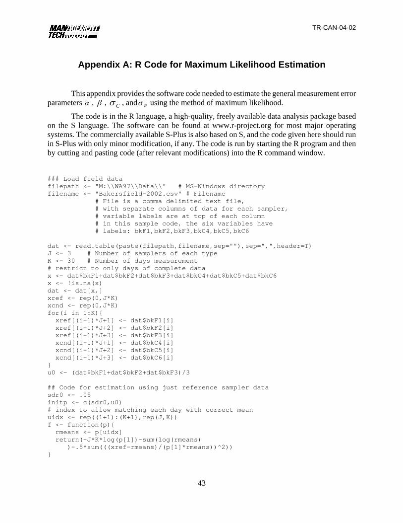
Appendix A: R Code for Maximum Likelihood Estimation
This appendix provides the software code needed to estimate the general measurement errorparameters , , , and using the method of maximum likelihood.α β Cσ Rσ
The code is in the R language, a high-quality, freely available data analysis package basedon the S language. The software can be found at www.r-project.org for most major operatingsystems. The commercially available S-Plus is also based on S, and the code given here should runin S-Plus with only minor modification, if any. The code is run by starting the R program and thenby cutting and pasting code (after relevant modifications) into the R command window.
### Load field datafilepath <- "M:\\WA97\\Data\\" # MS-Windows directoryfilename <- "Bakersfield-2002.csv" # Filename # File is a comma delimited text file,
# with separate columns of data for each sampler,# variable labels are at top of each column# in this sample code, the six variables have# labels: bkF1,bkF2,bkF3,bkC4,bkC5,bkC6
dat <- read.table(paste(filepath,filename,sep=""),sep=",",header=T)J <- 3 # Number of samplers of each typeK <- 30 # Number of days measurement# restrict to only days of complete datax <- dat$bkF1+dat$bkF2+dat$bkF3+dat$bkC4+dat$bkC5+dat$bkC6x <- !is.na(x)dat <- dat[x,]xref <- rep(0,J*K)xcnd <- rep(0,J*K)for(i in 1:K){ xref[(i-1)*J+1] <- dat$bkF1[i] xref[(i-1)*J+2] <- dat$bkF2[i] xref[(i-1)*J+3] <- dat$bkF3[i] xcnd[(i-1)*J+1] <- dat$bkC4[i] xcnd[(i-1)*J+2] <- dat$bkC5[i] xcnd[(i-1)*J+3] <- dat$bkC6[i]}u0 <- (dat$bkF1+dat$bkF2+dat$bkF3)/3
## Code for estimation using just reference sampler datasdr0 <- .05initp <- c(sdr0,u0)# index to allow matching each day with correct meanuidx <- rep((1+1):(K+1),rep(J,K)) f <- function(p){ rmeans <- p[uidx] return(-J*K*log(p[1])-sum(log(rmeans) )-.5*sum(((xref-rmeans)/(p[1]*rmeans))^2))}
TR-CAN-04-02
44
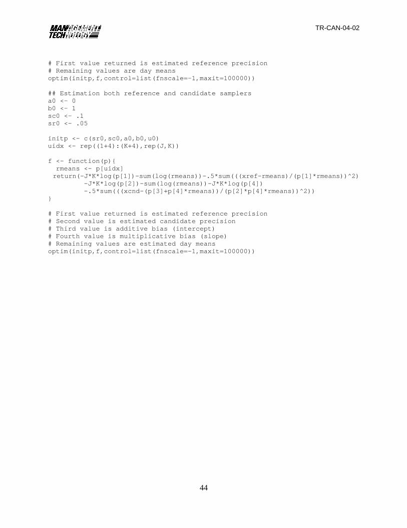
# First value returned is estimated reference precision# Remaining values are day meansoptim(initp,f,control=list(fnscale=-1,maxit=100000))
## Estimation both reference and candidate samplersa0 <- 0b0 <- 1sc0 <- .1sr0 <- .05
initp <- c(sr0,sc0,a0,b0,u0)uidx <- rep((1+4):(K+4),rep(J,K))
f <- function(p){ rmeans <- p[uidx] return(-J*K*log(p[1])-sum(log(rmeans))-.5*sum(((xref-rmeans)/(p[1]*rmeans))^2) -J*K*log(p[2])-sum(log(rmeans))-J*K*log(p[4]) -.5*sum(((xcnd-(p[3]+p[4]*rmeans))/(p[2]*p[4]*rmeans))^2))}
# First value returned is estimated reference precision# Second value is estimated candidate precision# Third value is additive bias (intercept)# Fourth value is multiplicative bias (slope)# Remaining values are estimated day meansoptim(initp,f,control=list(fnscale=-1,maxit=100000))
TR-CAN-04-02
45
2
CV σ σμ μ
= =
ˆ SCVX
=
2 2U UCVU Uσ σ σ= = =
2 2 2
1
UCV
UU
β σ σαα ββ
= =+ +
Appendix B: Precision and Variance
In this report, precision is used synonymously with standard deviation for the multiplicativemodel. This usage has developed through their equivalence for models considered by the DQOmethodology and for models of WA 76. With the addition of an additive bias (intercept) to themodel, the relationship is no longer exact, although the usage has been retained for consistency.These relationships are described in more detail below.
For measurements of mean , variance , the population coefficient of1,..., nX X μ 2σvariation (precision) is defined as
which is often estimated as
where is the sample standard deviation and is the sample mean. Note that the CV is unitlessS Xsince and have the same units.μ σ
For daily measurements of daily true value (realization of population1,..., nX X Uprocess), we assume measurement error model
1. , ork kX Uε=2. k kX Uα β ε= +
In the case of 1, the population mean (for that day) is and the variance is , so theU 2 2U σcoefficient of variation is
and so the CV, which is unitless, happens to equal , which has units.σIn the case of 2, the population mean is and the variance is , so theUα β+ 2 2U σ
coefficient of variation is

TR-CAN-04-02
46
which equals if . Therefore, when the intercept is non-zero, the standard deviation doesσ 0α =not exactly equal the coefficient of variation (although if then the CV might not be what one0α ≠would want to measure, since it then depends on leading to a different CV for each possible trueUdaily value. In such a situation, is probably more useful).σ