data representation - cs.sjtu.edu.cn

Data Representation

Continuous DataSampled DataDiscrete DatasetsCell Types

•vertex, line, triangle, quad, tetrahedron, hexahedron

Grid Types•Uniform, rectlinear, structured, Unstructured

Attributes•Scalar, Vector, Color, Tensor, Non-numerical

outline

Continuous Data versusDiscrete Data

•Continuous Data•Most scientific quantities are continuous in nature•Scientific Visualization, or scivis

•Discrete Data•E.g., text, images and others that can not be interpolated or scaled•Information Visualization, or infovis

•Continuous data, when represented by computers, are always in discrete form

•These are called “sampled data”•Originated from continuous data•Intended to approximate the continuous quantity through visualization

Continuous Data

2

2 )()('',

)()(),(

dx

xfdxf

dx

xdfxfxf

a: discontinuousfunction

b: first-order continuous function: first-order derivative is not continuous

c: high-order continuous function

Continuous Data

f is a d-dimension, c-valued functionD: function domainC: function co-domain

)....,()....,(

C

D

CD:

2121 dc

c

d

xxxfyyy

f

R

R

Continuous data can be modeled as:

Continuous Data

||f(p)-f(x)||

then

||p-x||

ifsuch that

0 0,

Cauchy criterion of continuity

Graphically, a function is continuous if the graph of the function is a connected surface without “holes” or “jumps”

A function is continuous of order k if the function itself and all its derivative up to order k are also continuous

In words, small changes in the input result in small changes in the output

Graphically, a function is continuous if the graph of the function is a connected surface without “holes” or “jumps”

In words, small changes in the input result in small changes in the output

•Geometric dimension: d• the space into which the function domain D is embedded•It is always 3 in the usual Euclidean space: d=3

•Topological dimension: s•The function domain D itself•A line or curve: s=1, d=3•A plane or curved surface: s=2, d=3

•Dataset dimension refers to the topological dimension•Function values in the co-domain are called dataset attributes•Attribute dimension: dimension of the function co-domain

f) C, (D,cD1. D: Function domain2. C: Function co-domain3. f: Function itself

Sampling and Reconstruction

fff i

~

Sampled data

• Sampling: from continuous dataset

to Sampled data

• Reconstruction:

from Sampled data

to recover/approximate

continuous dataset

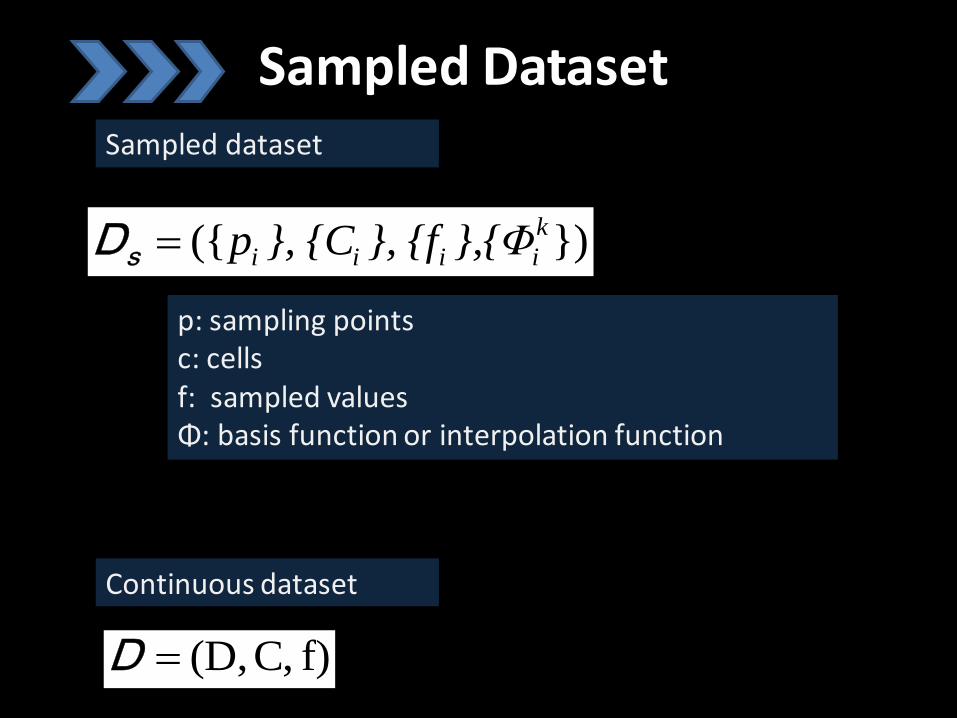
Sampled DatasetSampled dataset

f) C, (D,D

})({ k

iiii },{Φ}, {f}, {CpsD

Continuous dataset

1. p: sampling points2. c: cells 3. f: sampled values4. Φ: basis function or interpolation function

A signal domain is sampled in a grid that contains a set of cells defined by the sample points

Point,Cell, Grid

Sampling

Sampling

D

0

}....,{

,

21

ii

ji

d

d

i

cU

ji,cc

pppci

p RPoint

Cell

Grid

Reconstruction

function basis called is where

~

...}2,1{},

i

1

N

i

ii

i

ff

i{f

or interpolation function

Piecewise fitting: one cell one time

ReconstructionLinear basis function

rfrfrf

rr

rr

21

1

2

1

1

)1()(

,)(

,1)(

For 1-D line

P1 P2

0 r 1

reference cell

Basis Function

Basis function shall be orthonormal

1.Orthogonal: only vertex points within the same cell have contribution to the interpolated value2.Normal: the sum of the basic functions of the vertices shall be unity.

Basis FunctionLinear basis function

For 2-D quad

srsr

rssr

srsr

srsr

)1(),(

),(

)1(),(

)1)(1(),(

1

4

1

3

1

2

1

1

Sampled DatasetSampled dataset

f) C, (D,D

})({ k


Continuous dataset

p: sampling pointsc: cells f: sampled valuesΦ: basis function or interpolation function

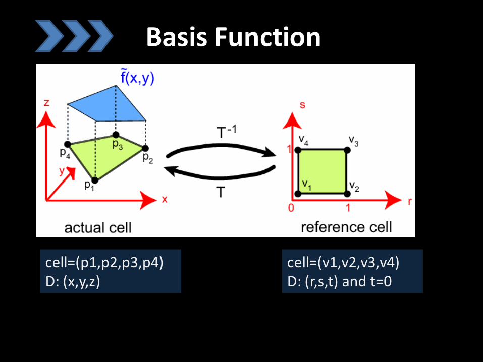
cell=(p1,p2,p3,p4)D: (x,y,z)

cell=(v1,v2,v3,v4)D: (r,s,t) and t=0

Basis Function

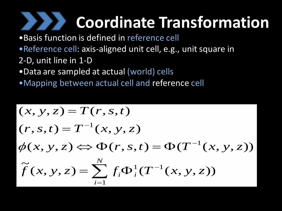
Coordinate Transformation•Basis function is defined in reference cell•Reference cell: axis-aligned unit cell, e.g., unit square in 2-D, unit line in 1-D•Data are sampled at actual (world) cells•Mapping between actual cell and reference cell

N

i

ii zyxTfzyxf

zyxTtsrzyx

zyxTtsr

tsrTzyx

1

11

1

1

)),,((),,(~

)),,((),,(),,(

),,(),,(

),,(),,(

Discrete Datasets

• A Grid = cells + sample points

• Sample Values at cell centers/vertices

• Basis functions

Cell types

• Vertex • Line• Triangle• Quad• Rectangle• Tetrahedron• Hexahedron• Parallelipiped• Pyramid• prism

Vertex

d=0

1),(

}{

0

1

1

sr

vc

• Vertex • Line• Triangle• Quad• Rectangle• Tetrahedron• Hexahedron• Parallelipiped• Pyramid• prism

• Vertex• Line• Triangle• Quad• Rectangle• Tetrahedron• Hexahedron• Parallelipiped• Pyramid• prism

Lined=1

2

12

1211

1

2

1

1

21

||||

)()(),,(

)(

1)(

},{

pp

ppppzyxT

rr

rr

vvc

Line (cont.)Actual line d=1

12

12

12

21

12

1

2211 ,,

xx

xxf

xx

xxff

xx

xxr

xpxpxp

Actual line d=2

2

12

2

12

121121

222111

)()(

))(())((

),(),,(),,(

yyxx

yyyyxxxxr

yxpyxpyxp


Triangled=2

2

13

131

2

12

121

1

1

3

1

2

1

1

321

||||

)()(

||||

)()(

),(),,(

),(

),(

1),(

},,{

pp

pppps

pp

ppppr

srzyxT

ssr

rsr

srsr

vvvc


Quadd=2

2

14

141

2

12

121

1

4

1

3

1

2

1

1

4321

||||

)()(

||||

)()(

)1(),(

),(

)1(),(

)1)(1(),(

},,,{

pp

pppps

pp

ppppr

srsr

rssr

srsr

srsr

vvvvc



Tetrahedrond=3

2

14

141

2

13

131

2

12

121

1

1

4

1

3

1

2

1

1

4321

||||

)()(

||||

)()(

||||

)()(

),,(),,(

),(

),(

),(

1),(

},,,{

pp

ppppt

pp

pppps

pp

ppppr

tsrzyxT

tsr

ssr

rsr

tsrsr

vvvvc


Hexahedrond=3

strsr

rstsr

tsrsr

tsrsr

trsr

trssr

tsrsr

tsrsr

vvvvvvvvc

)1(),(

),(

)1(),(

)1)(1(),(

)1)(1(),(

)1(),(

)1)(1(),(

)1)(1)(1(),(

},,,,,,,{

1

8

1

7

1

6

1

5

1

4

1

3

1

2

1

1

87654321


Hexahedron (cont.)d=3

2

18

181

2

14

141

2

12

121

1

||||

)()(

||||

)()(

||||

)()(

),,(),,(

pp

ppppt

pp

pppps

pp

ppppr

tsrzyxT

Effect of Reconstruction

Geometry:

Constant

Geometry:

Linear

Lighting:

Constant

Staircase

shading

Flat

Shading

Lighting:

Linear

--------- Smooth

(Gouraud)

shading

Effect of Reconstruction

Staircase Shading Flat Shading Smooth Shading

Grid types

• Grid is the pattern of cells in the data domain

• Grid is also called mesh

• Uniform grid

• Rectilinear grid

• Structured grid

• Unstructured grid

Uniform Grid

2-D 3-D

Uniform Grid•The simplest grid type•Domain D is usually an axis-aligned box

•Line segment for d=1•Rectangle for d=2•parallelepiped for d=3

•Sample points are equally distributed on every axis•Structured coordinates: the position of the sample points in the data domain are simply indicated by d integer coordinates (n1,..nd)•Simple to implement•Efficient to run (storage, memory and CPU)

Uniform Grid•Data points are simply stored in the increasing order of the indices, e.g, an 1-D array •Lexicographic order

213121

121

12

121

2

1

1

1

3,d If

mod

2,d If

)(

NNnNnni

)N (ni n

i/Nn

, orNnni

Nnnid

k

k

l

lk

Rectilinear Grid

2-D 3-D

Rectilinear Grid

•Domain D is also an axis-aligned box•However, the sampling step is not equal

•It is not as simple or as efficient as the uniform grid•However, improving modeling power

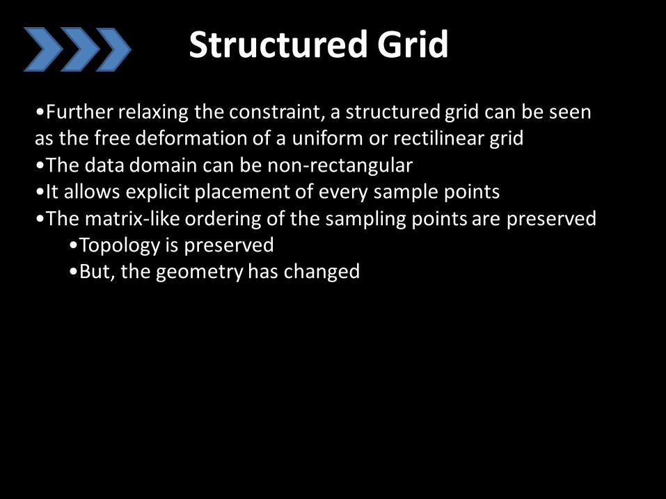
Structured Grid

•Further relaxing the constraint, a structured grid can be seen as the free deformation of a uniform or rectilinear grid•The data domain can be non-rectangular•It allows explicit placement of every sample points•The matrix-like ordering of the sampling points are preserved

•Topology is preserved•But, the geometry has changed

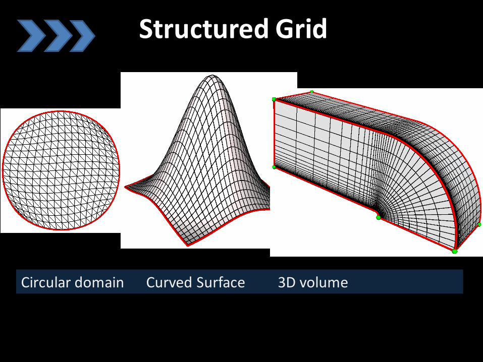
Structured Grid

Circular domain Curved Surface 3D volume

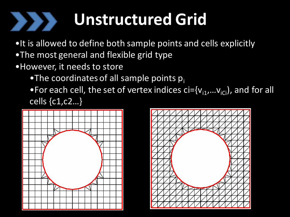
Unstructured Grid•It is allowed to define both sample points and cells explicitly•The most general and flexible grid type•However, it needs to store

•The coordinates of all sample points pi

•For each cell, the set of vertex indices ci={vi1,…viCi), and for all cells {c1,c2…}

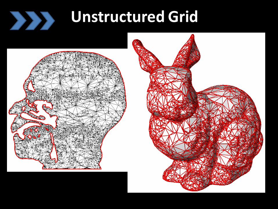
Unstructured Grid

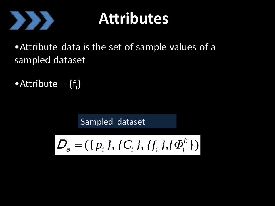
•Attribute data is the set of sample values of a sampled dataset

•Attribute = {fi}

})({ k


Sampled dataset

Attributes

Attribute Types

•Scalar Attribute

•Vector Attribute

•Color Attribute: c=3

•Tensor Attributes

•Non-Numerical Attributes

1

C

c

cR

3or ,2

C

cc

cR

•Scalar, Vector, Color, Tensor, Non-numerical

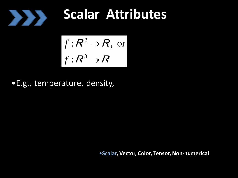
Scalar Attributes

•E.g., temperature, density,

RR

RR

3

2

:

or ,:

f

f


Vector Attributes

•E.g.,•Normal•Force•velocity

•A vector has a magnitude and orientation

3

2

RR

RR

3

2

:

or ,:

f

f


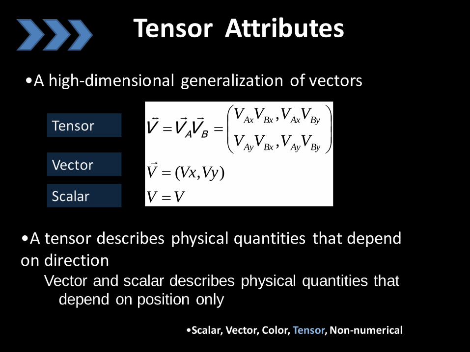
Tensor Attributes

•A high-dimensional generalization of vectors

VV

VyVxV

VVVV

VVVV

ByAyBxAy

ByAxBxAx

),(

,

,

BAVVVTensor

Vector

Scalar

•A tensor describes physical quantities that depend on direction

Vector and scalar describes physical quantities that

depend on position only


Tensor Attributes

•E.g. curvature of a 2-D surface

•E.g., diffusivity, conductivity, stress

Tensor


Non-numerical Attributes

•E.g. text, image, voice, and video•Data can not be interpolated•Therefore, the dataset has no basis function•Domain of information of visualization (infovis)

Scalar, Vector, Color, Tensor, Non-numerical

Color Attributes

•A special type of vector attributes with dimension c=3

•RGB system: convenient for hardware and implementation

R: red

G: green

B: blue

•HSV system: intuitive for human userH: Hue

S: Saturation

V: Value

RGB System

•Every color is represented as a mix of “pure” red, green and blue colors in different amount•Equal amounts of the three colors determines gray shades•RGB cube’s main diagonal line connecting the points (0,0,0) and (1,1,1) is the locus of all the grayscale value

RGB CubeR

G

B

yellow

magenta

Cyan

HSV System

•Hue: distinguish between different colors of different wavelengths, from red to blue•Saturation: represent the color of “purity”, or how much hue is diluted with white

S=1, pure, undiluted color

S=0, white

•Value: represent the brightness, or luminanceV=0, always dark

V=1, brightest color for a given H and S

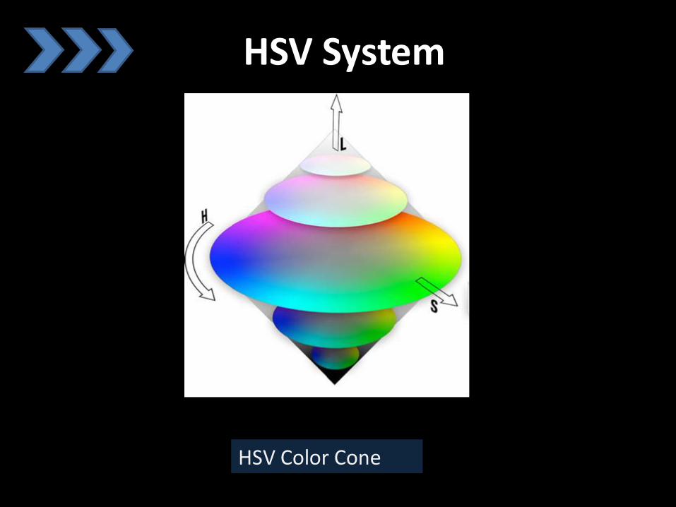
HSV System

HSV Color Cone

Color, Light, Electromagnetic Radiation

RGB to HSV•All values are in [0,1]

max=max(R,G,B)min=min(R,G,B)diff=max-min

•V = max•largest RGB component

•S = diff/max•For hue H, different cases

•H = (G-B)/diff if R=max•H =2+(B-R)/diff if G=max•H =4+(R-G)/diff if B=max•then H=H/6•H=H+1 if H < 0

•Exp: Full Green Color•(R,G,B)=(0,1,0) •(H,S,V)=(1/3, 1,1)

•Exp: Yellow Color•(R,G,B)=(1,1,0) •(H,S,V)=(1/6, 1, 1)

HSV to RGB

•huecase = {int} (h*6)•frac = 6*h – huecase

•lx= v*(1-s)•ly= v*(1-s*frac)•lz= v*(1-s(1-frac))

•huecase =6 (0<h<1/6): r=v, g=lz, b=lx•huecase =1 (1/6<h<2/6): r=ly, g=v, b=lx•huecase =2 (2/6<h<3/6): r=lx, g=v, b=lz•huecase =3 (3/6<h<4/6): r=lx, g=ly, b=v•huecase =4 (4/6<h<5/6): r=lz, g=lx, b=v•huecase =5 (5/6<h<1): r=v, g=lx, b=ly

•Exp: Full Green Color•(H,S,V)=(1/3,1,1) •(R,G,B)=(0,1,0)

•Exp: Yellow Color•(H,S,V)=(1/6,1,1) •(R,G,B)=(1,1,0)

Conclusion•Fundamental issues involved in representing data for visualization applications•A set of data cells •Data attributes, several types: scalar vector color and tensor•Basis function: constant and linear

Simplicity of implementation and direct support in the

graphics hardware

•Grid Types: uniform, rectilinear, structured and unstructured grids

data representation - cs.sjtu.edu.cn

Documents