data representation synthesis a dissertation...
TRANSCRIPT

DATA REPRESENTATION SYNTHESIS
A DISSERTATIONSUBMITTED TO THE DEPARTMENT OF COMPUTER SCIENCE
AND THE COMMITTEE ON GRADUATE STUDIESOF STANFORD UNIVERSITY
IN PARTIAL FULFILLMENT OF THE REQUIREMENTSFOR THE DEGREE OF
DOCTOR OF PHILOSOPHY
Peter HawkinsApril 2012

http://creativecommons.org/licenses/by-nc/3.0/us/
This dissertation is online at: http://purl.stanford.edu/zq724mz4389
© 2012 by Peter James Hawkins. All Rights Reserved.
Re-distributed by Stanford University under license with the author.
This work is licensed under a Creative Commons Attribution-Noncommercial 3.0 United States License.
ii

I certify that I have read this dissertation and that, in my opinion, it is fully adequatein scope and quality as a dissertation for the degree of Doctor of Philosophy.
Alex Aiken, Primary Adviser
I certify that I have read this dissertation and that, in my opinion, it is fully adequatein scope and quality as a dissertation for the degree of Doctor of Philosophy.
David Dill
I certify that I have read this dissertation and that, in my opinion, it is fully adequatein scope and quality as a dissertation for the degree of Doctor of Philosophy.
Kathleen Fisher
Approved for the Stanford University Committee on Graduate Studies.
Patricia J. Gumport, Vice Provost Graduate Education
This signature page was generated electronically upon submission of this dissertation in electronic format. An original signed hard copy of the signature page is on file inUniversity Archives.
iii

Abstract
This dissertation introduces Data Representation Synthesis, a technique for specifying combinations of datastructures with complex sharing in a manner that is both declarative and results in provably correct code. In ourapproach, abstract data types are specified using relational algebra and functional dependencies. We describe alanguage of decompositions that permit a programmer to specify different concrete representations for relations,and show that operations on concrete representations soundly implement their relational specification.
Decompositions also give new insight into the problem of writing safe and efficient concurrent code. Weintroduce lock placements, which describe, for each heap location, which lock guards the location, and underwhat circumstances. By incorporating lock placements into decompositions, a compiler can automatically ex-plore the space of possible legal data representations and locking strategies, while simultaneously guaranteeingcorrectness, serializability of relational operations, and deadlock-freedom.
It is easy to incorporate data representations synthesized by our compiler into existing systems, leadingto code that is simpler, correct by construction, and comparable in performance to the code it replaces. Wedescribe our experience with a prototype compiler; code generated by our system can easily be dropped intoexisting systems in place of complex hand-written implementations with comparable performance.
iv
Acknowledgements
I have been very fortunate to work with my advisor, Alex Aiken, whose mentorship and guidance has beeninstrumental in helping me develop as a researcher. Alex introduced me to many aspects of computer science,collaborated with me on a wide variety of new and exciting problems, and helped me navigate the shoals andrapids of the research world. Working in Alex’s group has always been fun and has taught me a great deal:many thanks go out to Michael Bauer, Sorav Bansal, Isil Dillig, Tom Dillig, Brian Hackett, Mayur Naik, AdamOliner, Eric Schkufza, Rahul Sharma, Sean Treichler, and Yichen Xie for all the interesting conversations andall the cups of coffee.
I am grateful for the opportunity to work with brilliant collaborators during my time at Stanford: KathleenFisher, Martin Rinard, and Mooly Sagiv. Their guidance and advice has taught me many different things aboutresearch and how to approach it, and I feel honored to have had the opportunity to work with them. I wouldespecially like to thank Kathleen, who served as my advisor during Alex’s absence, and as a friend and mentorthereafter. I would also like to thank my reading committee (Alex Aiken, David Dill, and Kathleen Fisher),and my oral committee (Alex Aiken, David Dill, Kathleen Fisher, Hector Garcia-Molina, and Stephen Sano)for their invaluable assistance.
During my time at Stanford, I have made many wonderful friends with whom I have shared many adventures.To all those who shared these experiences with me, especially my friends, family, and Mariangela: thank you.I couldn’t have done this without you.
v
Contents
Abstract iv
Acknowledgements v
1 Introduction 11.1 Dissertation Overview . . . . . . . . . . . . . . . . . . . . . . . . . . . . . . . . . . . . . 21.2 A Motivating Example . . . . . . . . . . . . . . . . . . . . . . . . . . . . . . . . . . . . . 2
1.2.1 Characteristics of a Good Data Representation . . . . . . . . . . . . . . . . . . . . 41.3 Data Representation Synthesis . . . . . . . . . . . . . . . . . . . . . . . . . . . . . . . . . 51.4 Databases and Programming With Relations . . . . . . . . . . . . . . . . . . . . . . . . . . 7
1.4.1 Relational Programming Constructs . . . . . . . . . . . . . . . . . . . . . . . . . . 81.5 Data Representation Synthesis and Verification . . . . . . . . . . . . . . . . . . . . . . . . 9
1.5.1 Static Analysis and Verification Techniques . . . . . . . . . . . . . . . . . . . . . . 91.6 Collaborators and Publications . . . . . . . . . . . . . . . . . . . . . . . . . . . . . . . . . 12
2 Data Representation Synthesis 132.1 Relational Abstraction . . . . . . . . . . . . . . . . . . . . . . . . . . . . . . . . . . . . . 142.2 Decompositions and Decomposition Instances . . . . . . . . . . . . . . . . . . . . . . . . . 16
2.2.1 Decompositions . . . . . . . . . . . . . . . . . . . . . . . . . . . . . . . . . . . . 162.2.2 Abstraction Function . . . . . . . . . . . . . . . . . . . . . . . . . . . . . . . . . . 192.2.3 Well-formed Decomposition Instances . . . . . . . . . . . . . . . . . . . . . . . . . 192.2.4 Adequacy of Decompositions . . . . . . . . . . . . . . . . . . . . . . . . . . . . . 20
2.3 Querying and Updating Decomposed Relations . . . . . . . . . . . . . . . . . . . . . . . . 222.3.1 Queries and Query Plans . . . . . . . . . . . . . . . . . . . . . . . . . . . . . . . . 222.3.2 Query Validity . . . . . . . . . . . . . . . . . . . . . . . . . . . . . . . . . . . . . 242.3.3 Query Planner . . . . . . . . . . . . . . . . . . . . . . . . . . . . . . . . . . . . . 262.3.4 Mutation: Empty and Insert Operations . . . . . . . . . . . . . . . . . . . . . . . . 262.3.5 Mutation: Removal and Update Operations . . . . . . . . . . . . . . . . . . . . . . 272.3.6 Soundness of Relational Operations . . . . . . . . . . . . . . . . . . . . . . . . . . 29
vi

2.4 Autotuner . . . . . . . . . . . . . . . . . . . . . . . . . . . . . . . . . . . . . . . . . . . . 302.5 Experiments . . . . . . . . . . . . . . . . . . . . . . . . . . . . . . . . . . . . . . . . . . . 30
2.5.1 Microbenchmarks . . . . . . . . . . . . . . . . . . . . . . . . . . . . . . . . . . . 312.5.2 Data Representation Synthesis in Existing Systems . . . . . . . . . . . . . . . . . . 33
2.6 Proofs of Theorems . . . . . . . . . . . . . . . . . . . . . . . . . . . . . . . . . . . . . . . 352.6.1 Soundness of Adequacy . . . . . . . . . . . . . . . . . . . . . . . . . . . . . . . . 352.6.2 Soundness of Queries . . . . . . . . . . . . . . . . . . . . . . . . . . . . . . . . . . 362.6.3 Soundness of Mutations . . . . . . . . . . . . . . . . . . . . . . . . . . . . . . . . 38
3 Lock Placements 433.1 Flat Maps . . . . . . . . . . . . . . . . . . . . . . . . . . . . . . . . . . . . . . . . . . . . 45
3.1.1 Concrete Semantics . . . . . . . . . . . . . . . . . . . . . . . . . . . . . . . . . . . 463.1.2 Lock Placements . . . . . . . . . . . . . . . . . . . . . . . . . . . . . . . . . . . . 473.1.3 Well-Locked Transactions . . . . . . . . . . . . . . . . . . . . . . . . . . . . . . . 493.1.4 Serializability of Well-Locked Transactions . . . . . . . . . . . . . . . . . . . . . . 513.1.5 Shared/Exclusive Logical Locks . . . . . . . . . . . . . . . . . . . . . . . . . . . . 53
3.2 Mutable Tree-Structured Heaps . . . . . . . . . . . . . . . . . . . . . . . . . . . . . . . . . 533.2.1 Lock Placements . . . . . . . . . . . . . . . . . . . . . . . . . . . . . . . . . . . . 543.2.2 Well-Locked Transactions . . . . . . . . . . . . . . . . . . . . . . . . . . . . . . . 57
3.3 Transactions on Decomposition Heaps . . . . . . . . . . . . . . . . . . . . . . . . . . . . . 613.3.1 Lock Placements . . . . . . . . . . . . . . . . . . . . . . . . . . . . . . . . . . . . 633.3.2 Well-Locked Transactions . . . . . . . . . . . . . . . . . . . . . . . . . . . . . . . 65
3.4 Related Work . . . . . . . . . . . . . . . . . . . . . . . . . . . . . . . . . . . . . . . . . . 68
4 Concurrent Data Representation Synthesis 704.1 Concurrent Relations . . . . . . . . . . . . . . . . . . . . . . . . . . . . . . . . . . . . . . 724.2 A Taxonomy of Concurrent Containers . . . . . . . . . . . . . . . . . . . . . . . . . . . . . 73
4.2.1 Concurrency Safety and Consistency . . . . . . . . . . . . . . . . . . . . . . . . . 734.3 Concurrent Decompositions . . . . . . . . . . . . . . . . . . . . . . . . . . . . . . . . . . 75
4.3.1 Logical Locks, Transactions, and Serializability . . . . . . . . . . . . . . . . . . . . 754.3.2 Physical Locks and Lock Placements . . . . . . . . . . . . . . . . . . . . . . . . . 764.3.3 Lock Striping . . . . . . . . . . . . . . . . . . . . . . . . . . . . . . . . . . . . . . 794.3.4 Speculative Lock Placements . . . . . . . . . . . . . . . . . . . . . . . . . . . . . . 80
4.4 Query Planning and Lock Ordering . . . . . . . . . . . . . . . . . . . . . . . . . . . . . . . 814.4.1 Deadlock-Freedom and Lock Ordering . . . . . . . . . . . . . . . . . . . . . . . . 814.4.2 Query Language . . . . . . . . . . . . . . . . . . . . . . . . . . . . . . . . . . . . 82
4.5 Experimental Evaluation . . . . . . . . . . . . . . . . . . . . . . . . . . . . . . . . . . . . 864.5.1 Autotuner . . . . . . . . . . . . . . . . . . . . . . . . . . . . . . . . . . . . . . . . 86
vii

4.5.2 Graph Benchmark . . . . . . . . . . . . . . . . . . . . . . . . . . . . . . . . . . . 884.5.3 Concurrent Cache Benchmark . . . . . . . . . . . . . . . . . . . . . . . . . . . . . 90
4.6 Discussion and Related Work . . . . . . . . . . . . . . . . . . . . . . . . . . . . . . . . . . 95
5 Conclusions 96
Bibliography 98
viii

List of Tables
2.1 Reduction in code size from applying synthesis . . . . . . . . . . . . . . . . . . . . . . . . 33
4.1 Concurrency safety properties of selected containers from the JDK . . . . . . . . . . . . . . 74
ix

List of Figures
1.1 Extracts from the definitions of super_block and inode . . . . . . . . . . . . . . . . . . . 31.2 A typical Linux inode cache heap state . . . . . . . . . . . . . . . . . . . . . . . . . . . . 41.3 Schematic of Data Representation Synthesis. . . . . . . . . . . . . . . . . . . . . . . . . . 6
2.1 The C++ class generated for the scheduler relation. . . . . . . . . . . . . . . . . . . . . . . 162.2 Data representation for a process scheduler . . . . . . . . . . . . . . . . . . . . . . . . . . 172.3 Grammar of the decomposition language. . . . . . . . . . . . . . . . . . . . . . . . . . . . 182.4 Grammar of decomposition instances. . . . . . . . . . . . . . . . . . . . . . . . . . . . . . 182.5 Process scheduler example written in let-notation . . . . . . . . . . . . . . . . . . . . . . . 192.6 The abstraction functions ↵(d,�) and ↵(p,�) . . . . . . . . . . . . . . . . . . . . . . . . . 202.7 Well-formed decomposition instances . . . . . . . . . . . . . . . . . . . . . . . . . . . . . 202.8 Adequate decompositions . . . . . . . . . . . . . . . . . . . . . . . . . . . . . . . . . . . . 212.9 Query plan operators . . . . . . . . . . . . . . . . . . . . . . . . . . . . . . . . . . . . . . 232.10 Valid query plans . . . . . . . . . . . . . . . . . . . . . . . . . . . . . . . . . . . . . . . . 252.11 Example of insertion and removal . . . . . . . . . . . . . . . . . . . . . . . . . . . . . . . 272.12 Two cuts of a decomposition . . . . . . . . . . . . . . . . . . . . . . . . . . . . . . . . . . 282.13 Depth-first search algorithm . . . . . . . . . . . . . . . . . . . . . . . . . . . . . . . . . . 312.14 Elapsed times for directed graph benchmarks . . . . . . . . . . . . . . . . . . . . . . . . . 322.15 Selected decompositions for the directed graph benchmark . . . . . . . . . . . . . . . . . . 332.16 Autotuner results . . . . . . . . . . . . . . . . . . . . . . . . . . . . . . . . . . . . . . . . 34
3.1 Locations, Lock Placements, Transaction Operations . . . . . . . . . . . . . . . . . . . . . 453.2 Concrete semantics of flat heap transactions . . . . . . . . . . . . . . . . . . . . . . . . . . 463.3 Transaction traces that observe the same memory locations under different lock placements . 473.4 Traces that read a memory location under a speculative lock placement . . . . . . . . . . . . 493.5 Well-locked transaction operations on flat maps . . . . . . . . . . . . . . . . . . . . . . . . 503.6 Tree transactions . . . . . . . . . . . . . . . . . . . . . . . . . . . . . . . . . . . . . . . . 543.7 Two examples of tree-structured heaps . . . . . . . . . . . . . . . . . . . . . . . . . . . . . 553.8 Transaction traces that add a new edge under three different lock placements . . . . . . . . . 56
x

3.9 Well-locked tree heap operations . . . . . . . . . . . . . . . . . . . . . . . . . . . . . . . . 583.10 A decomposition heap shape and a corresponding instance . . . . . . . . . . . . . . . . . . 623.11 Transactions on decomposition heaps. . . . . . . . . . . . . . . . . . . . . . . . . . . . . . 633.12 Example transactions that add a new node to a decomposition heap instance . . . . . . . . . 643.13 Well-locked decomposition operations . . . . . . . . . . . . . . . . . . . . . . . . . . . . . 66
4.1 A decomposition representing a directory tree relation . . . . . . . . . . . . . . . . . . . . . 764.2 Three concurrent decompositions for a directed graph relation . . . . . . . . . . . . . . . . 774.3 The concurrent query language . . . . . . . . . . . . . . . . . . . . . . . . . . . . . . . . . 824.4 Throughput/scalability curves for a selection of decompositions . . . . . . . . . . . . . . . 874.5 Scala code implementing a concurrent cache . . . . . . . . . . . . . . . . . . . . . . . . . . 914.6 The interface to the concurrent cache relation generated by the compiler . . . . . . . . . . . 924.7 Concurrent decompositions for the cache benchmark . . . . . . . . . . . . . . . . . . . . . 934.8 Throughput/scalability curves for a selection of concurrent decompositions . . . . . . . . . 94
xi

Chapter 1
Introduction
By automatically synthesizing the low-level representation of a program’s data from a high-level relationaldescription, we can obtain code that is simpler, correct by construction, and comparable in performance to thehandwritten code that it replaces.
Almost every non-trivial program represents its data internally using dynamically-allocated data structures,collectively called the heap. One of the first things a programmer must do when implementing a systemis commit to a particular choice of heap data structures that represent the system’s state. A choice of datarepresentation must meet several requirements: the representation must support all of the operations requiredby the code, the data structures must be efficient for the workload, and the implementation must be correct.
Whatever the choice of data structures, it has a pervasive influence on the subsequent code, and asrequirements evolve it is difficult and tedious to change the data structures to match. Extending or changingthe existing data structures to support a new requirement may require many changes throughout the code.For a data representation to be correct, data structure invariants must be enforced by every piece of code thatmanipulates the heap. Invariants on multiple data structures with complex patterns of sharing are hard to state,difficult to enforce, and easy to get wrong.
To address this problem this dissertation proposes a method termed data representation synthesis. In ourapproach a data structure client describes and manipulates data at a high level as relations; a data structuredesigner then provides decompositions which describe how those relations should be represented in memoryas a combination of primitive data structures. Our compiler RELC takes a relation and its decomposition andemits correct and efficient low-level code that implements the relational interface. As the programmer may notalways know the best decomposition for a particular relation, we describe an autotuner, which automaticallyidentifies a good decomposition for a particular relation and a particular workload.
Synthesis allows programmers to describe and manipulate data at a high level as relations, while givingcontrol of how relations are represented physically in memory. By abstracting data from its representation,programmers no longer prematurely commit to a particular representation of data. If programmers want tochange or extend their choice of data structures, they need only change the decomposition; the code that
1

CHAPTER 1. INTRODUCTION 2
uses the relation need not change at all. Synthesized representations are correct by construction; so long asthe programmer conforms to the relational specification, invariants on the synthesized data structures areautomatically maintained.
1.1 Dissertation Overview
For the balance of this chapter we describe data representation synthesis informally, motivated by a runningexample taken from the Linux kernel, and discuss how our approach relates to the extensive literature ondescribing and reasoning about the heap.
Chapter 2 formally describes data representation synthesis, which allows us to specify combinations of datastructures with complex sharing in a manner that is both declarative and results in provably correct code. In ourapproach, abstract data types are specified using relational algebra and functional dependencies. We describe alanguage of decompositions that permit the user to specify different concrete representations for relations, andshow that operations on concrete representations soundly implement their relational specification. We describeour experience incorporating data representations synthesized by our compiler into existing systems, leadingto code that is simpler, correct, and comparable in performance to the code it replaces.
Chapter 3 and Chapter 4 extend data representation synthesis to support concurrent access from multiplethreads. One of the primary benefits of the decomposition language is that it provides a powerful staticdescription of the heap, which we leverage to reason about concurrent data structures protected by locks.Chapter 3 introduces the abstract concept of a lock placement, which maps locations in the heap onto the locksthat protect them. Lock placements can describe a wide variety of both conservative and speculative lockingstrategies. A prerequisite for defining and reasoning about a lock placement is a description of the aliasingpatterns in the heap; we progressively consider lock placements for a sequence of increasingly complicatedheaps, applying lock placements to a class of flat maps, to tree-like heaps, and culminating in decompositionheaps. Chapter 4 applies the concept of a lock placement in the context of synthesis, yielding a completeconcurrent data representation system, and presents experimental results on a variety of benchmarks.
1.2 A Motivating Example
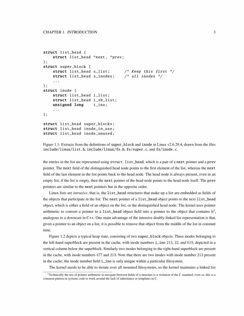
To motivate data representation synthesis, we begin with an example drawn from the Linux kernel. One of thekernel’s functions is to maintain a cache in memory of information about filesystems and files on disk. Thekernel represents each mounted filesystem in memory as a super_block object, and represents each file as aninode object. The kernel maintains a variety of data structures that link super_block and inode objects,each to support a different access pattern. Figure 1.1 shows extracts from the code that defines super_blockand inode, focusing on the data structures that allow us to navigate between them.
Each super_block and inode object participates in a number of linked lists. Most linked lists in theLinux kernel are circular, doubly-linked lists, with a distinguished head node. Both the head of the list and
CHAPTER 1. INTRODUCTION 3
struct list_head {struct list_head *next, *prev;
};struct super_block {
struct list_head s_list; /* Keep this first */
struct list_head s_inodes; /* all inodes */
...};struct inode {
struct list_head i_list;struct list_head i_sb_list;unsigned long i_ino;...
};
struct list_head super_blocks;struct list_head inode_in_use;struct list_head inode_unused;
Figure 1.1: Extracts from the definitions of super_block and inode in Linux v2.6.29.4, drawn from the filesinclude/linux/list.h, include/linux/fs.h, fs/super.c, and fs/inode.c.
the entries in the list are represented using struct list_head, which is a pair of a next pointer and a prevpointer. The next field of the distinguished head node points to the first element of the list, whereas the nextfield of the last element in the list points back to the head node. The head node is always present, even in anempty list; if the list is empty, then the next pointer of the head node points to the head node itself. The prevpointers are similar to the next pointers but in the opposite order.
Linux lists are intrusive, that is, the list_head structures that make up a list are embedded as fields ofthe objects that participate in the list. The next pointer of a list_head object points to the next list_headobject, which is either a field of an object on the list, or the distinguished head node. The kernel uses pointerarithmetic to convert a pointer to a list_head object field into a pointer to the object that contains it1,analogous to a downcast in C++. One main advantage of the intrusive doubly-linked list representation is that,given a pointer to an object on a list, it is possible to remove that object from the middle of the list in constanttime.
Figure 1.2 depicts a typical heap state, consisting of two super_block objects. Three inodes belonging tothe left-hand superblock are present in the cache, with inode numbers i_ino 213, 22, and 619, depicted in avertical column below the superblock. Similarly two inodes belonging to the right-hand superblock are presentin the cache, with inode numbers 477 and 213. Note that there are two inodes with inode number 213 presentin the cache; the inode number field i_ino is only unique within a particular filesystem.
The kernel needs to be able to iterate over all mounted filesystems, so the kernel maintains a linked list1Technically the use of pointer arithmetic to navigate between fields of a structure is a violation of the C standard; even so, this is a
common pattern in systems code to work around the lack of inheritance or templates in C.

CHAPTER 1. INTRODUCTION 4
super_blocks
super_block
s_lists_inodes
super_block
s_lists_inodes
inode_in_use
inode
i_list
i_sb_list
i_ino: 213
inode
i_list
i_sb_list
i_ino: 477
inode_unused
inode
i_list
i_sb_list
i_ino: 22
inode
i_list
i_sb_list
i_ino: 213
inode
i_list
i_sb_list
i_ino: 619
Figure 1.2: A typical Linux inode cache heap state. inode objects simultaneously participate in multiplecircular lists. Different line types denote different lists. Only the next edges of each list are shown; we omitthe prev edges for clarity.
of all of the super_block objects in memory. The global variable super_blocks is the distinguished headnode of the list, whereas the s_list fields of the super_block objects contain the pointers that form thespine of the list.
When unmounting a filesystem the kernel needs to find all inode objects belonging to that filesystemand evict them from the cache. To support efficient iteration over a filesystem’s inode objects, for eachsuper_block the kernel maintains a list of inode objects belonging to that filesystem. The distinguishedhead node of the list is the s_inodes field of the super_block, whereas the spine of the list is representedusing the i_sb_list fields of the inode objects.
Since there is usually far too much filesystem metadata to keep in memory, the inode objects in memoryare only a cache for the metadata on the disk. When the cache fills up, the kernel makes space in the cacheby evicting inode objects that have not been used recently. To support cache eviction each inode is also oneither of two global lists of inode objects: inode_in_use, if the inode is in use, or inode_unused, if theinode is unused. The kernel keeps the inode_unused list in an approximate Least-Recently-Used order; tofree space the kernel walks along the list of unused inodes evicting nodes until sufficient space is available.
1.2.1 Characteristics of a Good Data Representation
Are the Linux kernel’s data structures a good representation of an inode cache? To answer this question, wemust first characterize what we want from a data representation; ideally, a representation of data should satisfy

CHAPTER 1. INTRODUCTION 5
the following criteria:
• The data representation must provide a correct implementation of all operations required by client code.
• The implementation must be efficient for the access patterns that occur in practice.
• As the requirements on the data representation change, it should be easy to evolve the code to match.
• It should be easy to reason about the correctness of clients of a data representation.
The inode cache by definition supports all of the operations required by the Linux kernel. The implemen-tation is also quite efficient for the access patterns made by the kernel; in particular we can efficiently
• iterate over all super_block objects,
• given a particular super_block object, iterate over all inode objects belonging to that filesystem,
• iterate over unused inode objects on all filesystems in Least-Recently-Used order,
• add and remove super_block and inode objects from the cache, and
• change the state of an inode from used to unused or vice versa.
However it is not a particularly easy task to reason formally or informally about either the inode cacheor its clients. There is no real abstraction boundary between the data structures of the cache and its clients,and nowhere in the code is there a specification of precisely what the invariants of the inode cache datastructures are. It is therefore difficult to reason in a modular way about the correctness of the cache and itsclients. Because of the lack of abstraction, the choice of data structures has a pervasive influence on the rest ofthe code, and as requirements evolve it would be difficult and tedious to change the data structures to match.
Furthermore, invariants on multiple, overlapping data structures that represent different views of the samedata are hard to state, difficult to enforce, and easy to get wrong. For example, the kernel maintains theinvariants that every inode is present on its parent super_block’s list of children, and that every inode is onexactly one of the inode_in_use or inode_unused lists. Such invariants must be enforced by every pieceof code that manipulates the inode cache data structures. It would be easy to forget a case, say by failing tomove an inode to the appropriate list when changing its state, or by failing to remove an inode from theper-state list when evicting it from the cache. Invariants of this nature require deep knowledge about the heap’sstructure, and are difficult to enforce through existing static analysis or verification techniques.
1.3 Data Representation Synthesis
In this dissertation we propose a different approach, called data representation synthesis, depicted in Figure 1.3.In our approach a data structure client writes code that describes and manipulates data at a high level asrelations; a data structure designer then provides decompositions which describe how those relations should be

CHAPTER 1. INTRODUCTION 6
RELCSynthesis
hsb, inode, inuseisb, inode ! inuse
Relational Specification
x
y
z
w
inuse
sb
inuse
inode
sb, inode
Decomposition
class inode_relation {void insert(...);bool query(...);void update(...);void remove(...);};
Low-Level Implementation
Figure 1.3: Schematic of Data Representation Synthesis.
represented in memory as a combination of primitive data structures. Our compiler RELC takes a relation andits decomposition and synthesizes correct and efficient low-level code that implements the relational interface.
Synthesis allows programmers to describe and manipulate data at a high level as relations, while givingcontrol of how relations are represented physically in memory. By abstracting data from its representation,programmers no longer prematurely commit to a particular representation of data. If programmers want tochange or extend their choice of data structures, they need only change the decomposition; the code thatuses the relation need not change at all. Synthesized representations are correct by construction; so long asthe programmer conforms to the relational specification, invariants on the synthesized data structures areautomatically maintained.
Despite its apparent complexity, our key observation is that we can model the Linux inode cache as arelation with four columns {sb, inode,nr , inuse}. Each entry in the relation is a tuple of a super_blockobject (sb), an inode object (inode), the inode number (nr ), and a boolean indicating whether the inode is inuse (inuse). Not every such relation represents a valid inode cache; all meaningful cache relations satisfya pair of functional dependencies sb,nr ! inode and inode ! sb,nr , inuse. The functional dependenciesimply that there is at most one inode object with a given nr belonging to any given superblock sb; furthereach inode object has a unique superblock sb, inode number nr , and inuse state.
There are many possible representations of a relation; a data structure designer specifies a particular choiceof representation using a decomposition, which describes how to assemble container data structures froma library into a representation of the relation. It is the task of the compiler to generate implementations ofoperations to query and modify the relation, specialized to the particular decomposition. Different choices ofdecomposition will lead to different performance trade-offs. If the data structure designer does not know thebest decomposition or does not want to specify a decomposition by hand, then an autotuner can automaticallyexplore the space of possible decompositions to find a good decomposition for a particular workload.

CHAPTER 1. INTRODUCTION 7
1.4 Databases and Programming With Relations
The idea of representing data using relations is not new, dating back to the work of Codd [1970]. Relations andrelational algebra underlie the field of relational databases. Our insight is that relations are a good abstractionfor the kinds of heap data structures that occur in systems code, and unlike a typical relational database we cangive the programmer fine-grained control over the underlying representation via the decomposition language.
Classical relational databases represent a table as a list of tuples, together with one or more auxiliary indicesthat allow particular tuples to be located efficiently. Often clients have little control of how data is represented,beyond specifying the set of auxiliary indices. Since a database table must be capable of representing anypossible relation, databases are limited in how much they can specialize the representations of tables byleveraging properties of the data, such as functional dependencies. Traditional databases also usually do notassume that the complete set of queries will be known in advance, which limits how much a database canspecialize its representation to the query workload.
Recently there has been much interest in column-oriented databases, in which data is organized in columns,rather than in rows as is traditional. The MonetDB [Boncz and Kersten, 1999] and MonetDB/X100 [Bonczet al., 2005] pioneered the area of modern column-oriented databases. Column-oriented databases havesubsequently been explored in the context of the C-Store database [Stonebraker et al., 2005; Abadi et al.,2006]. Experimental evidence suggests that such specialized databases can perform orders of magnitude betterthan a conventional RDBMS for particular tasks, and a variety of authors have argued that the era of theone-size-fits-all row-oriented database is coming to an end [Stonebraker et al., 2007a,b; Abadi et al., 2008].This dissertation supports the same agenda in the context of in-memory data, demonstrating that there issignificant value to customizing the representation of data to a particular workload.
Most relational databases focus primarily on on-disk representations for data, optimizing to minimizeI/O workload. Since our goal is to synthesize in-memory data structures, many of the traditional databaseconstraints do not apply. Researchers have investigated specialized databases that operate entirely in mainmemory [DeWitt et al., 1984; Garcia-Molina and Salem, 1992], a topic that has seen a recent revival of interest[Ousterhout et al., 2010]. Most main memory databases in the literature represent data using variants of theB+-tree or T-tree index structures [Lehman and Carey, 1986], or one of their refinements [Rao and Ross, 1999,2000; Lu et al., 2000; Bin, 2003]. Evidence from a variety of systems [Lehman et al., 1992; Baulier et al., 1999;TimesTen, 1999] indicates that substantial performance improvements over traditional on-disk databases arepossible by tailoring the indexing structures of a database to an in-memory environment, even when the entiredatabase is small enough to fit in cache. Our work takes the trend a step further by providing a decompositionlanguage that allows a programmer to describe and generate highly specialized in-memory implementations ofa relation, thereby extracting the best possible performance.
Unlike a traditional database, in data representation synthesis the compiler knows the set of queries atcompile time, and we can specify custom representations tailored to the particular relation and the queryworkload using the decomposition language. Since our goal is to replace hand-written data structure code, ourcompiler eliminates much of the overhead of query evaluation by generating code for each query specialized

CHAPTER 1. INTRODUCTION 8
to the decomposition. Synthesized relations are correct by construction; provided that the client code obeys thefunctional dependencies of the relational specification, we show that the code generated by the compiler is afaithful implementation of the relational specification.
A novel aspect of our approach compared to a traditional database is that our relations can have specifiedrestrictions (specifically, functional dependencies). These restrictions, together with the fact that in the context ofcompilation the set of possible queries is known in advance, enable a wider range of possible implementations,particularly representations in which objects are shared between multiple different indices.
Beginning with Cohen and Campbell [1993] researchers have proposed light-weight in-memory databases,which compile relational abstract data types into combinations of container data structures. Batory and Thomas[1997] and the subsequent extensions of their work [Smaragdakis and Batory, 1997; Batory et al., 2000] alsoinvestigate light-weight databases, including language extensions to support relations, and techniques forassisting the programmer in choosing a good representation. Rothamel and Liu [2007] also describe a relationalabstract data type, where the underlying implementation may adapt based on observed usage patterns. Wepresent the first formal results, based on a formally-specified decomposition language capable of representingsharing, together with adequacy conditions that characterize sensible representations of a relation. We showthat our compiler generates code that is correct, and we report our experience with an implementation. Finally,we extend our synthesis approach to support shared-memory concurrency using locks.
We also describe a dynamic autotuner that can automatically synthesize the best decomposition for aparticular relation, and we present our experience with a full implementation of these techniques in practice.The autotuner framework has a similar goal to AutoAdmin [Chaudhuri and Narasayya, 1997]. AutoAdmintakes a set of tables, together with a distribution of input queries, and identifies a set of indices that are predictedto produce the best overall performance under the query optimizer’s cost model. The details differ because ourdecomposition and query languages are unlike those of a conventional database.
Synthesizing specialized data representations from a relational description has previously been consideredin other domains. The Bernoulli project [Kotlyar et al., 1997; Ahmed et al., 2000] investigated transformingdense matrix computations into implementations tailored to specific sparse representations as a technique forhandling the proliferation of complicated sparse representations.
1.4.1 Relational Programming Constructs
Many authors propose adding relations to both general- and special-purpose programming languages (e.g.,[Bierman and Wren, 2005; Meijer et al., 2006; Rothamel and Liu, 2007; Vaziri et al., 2007]). We focus on theorthogonal problem of generating efficient implementations for a relational abstraction. Data models such asEntity-Relationship diagrams and the Unified Modeling Language also rely heavily on relations. One potentialapplication of our technique is to close the gap between modeling languages and implementations.
The problem of automatic data structure selection was first explored in SETL [Schonberg et al., 1979;Paige and Henglein, 1987; Cai and Paige, 1991]; recent work has also explored automatic selection of Javacollection implementations [Shacham et al., 2009]. The SETL representation sublanguage [Dewar et al.,

CHAPTER 1. INTRODUCTION 9
1979] maps abstract SETL set and map objects to implementations, although the details are quite differentfrom our work. Unlike SETL, we handle relations of arbitrary arity, using functional dependencies to enforcesharing invariants. In SETL, set representations are dynamically embedded into carrier sets under the controlof the runtime system, while by contrast our compiler synthesizes low-level representations for a specificdecomposition with no runtime overhead.
1.5 Data Representation Synthesis and Verification
Reasoning about the heap is a fundamental building block of tools that reason about and transform programs;despite decades of research, reasoning automatically and precisely about the heap is an extremely challengingtask. Data representation synthesis gives us new insight into the problem of pointer analysis. Relations are aconvenient abstraction for encapsulating a collection of data structures. This encapsulation allows us to stateand guarantee sharing properties of data structures, even properties that would be difficult to verify on similarcode written by hand.
Consider the task of adding a fresh inode into the inode cache. To do so in the original Linux formulationrequires two operations—firstly, the inode must be added the list of inode objects belonging to its parentsuper_block. Secondly, the inodemust be added to one of the two lists inode_in_use and inode_unused,depending on whether the inode is in use or not. It is the programmer’s responsibility to keep the data structuresconsistent by ensuring that an inode is on a superblock’s list of children if and only if it is also on exactly oneof the in-use or unused lists. Stating such aliasing properties is difficult, and checking them is at the forefrontof shape analysis techniques. In the synthesis context, the code generated by the compiler maintains the correctaliasing automatically—since we have proven the translation correct, no additional verification of the generatedcode is required.
There is a large body of literature devoted to the problem of analyzing and reasoning about pointer-manipulating code. We briefly survey conventional approaches to reasoning about the heap, and show that oursynthesis approach is a compelling alternative.
1.5.1 Static Analysis and Verification Techniques
Researchers have developed many techniques for reasoning about pointer-manipulating code, including bothfully-automated techniques such as points-to and shape analyses, and partially-automated techniques based ondecision procedures and proof assistants. Each approach differs in its level of automation, its level of precision,and its computational complexity.
Alias and Points-To Analyses The most common types of pointer analysis are alias analyses and points-toanalyses. Alias analyses attempt to determine whether two expressions in a program may refer to the sameobject at run time. Points-to analyses attempt to determine which object names each pointer expressionmay point to at run time. Pointer analyses are broadly classified by how pointer expressions are named

CHAPTER 1. INTRODUCTION 10
(context-sensitivity), how objects are named (context-sensitivity, object-sensitivity), and whether the flow ofinformation in the analysis respects the control flow of the program (inclusion-based versus unification-based,flow-sensitivity). Influential examples of pointer analyses from the literature include the works of Weihl[1980], Landi and Ryder [1992], Deutsch [1992], Landi et al. [1993], Emami et al. [1994], Andersen [1994],Steensgaard [1996], Wilson and Lam [1995], Fähndrich et al. [2000], Das [2000], and Whaley and Lam [2004].
Although alias and points-to analyses are essential building blocks for a wide range of optimizing compilers,bug-finding tools, and program-understanding tools, neither technique has the precision necessary for generalverification problems. With very few exceptions, all alias and points-to analyses lose precision when reasoningabout programs that manipulate recursive data structures. Since object and expression contexts can be ofunbounded size in the presence of recursion, almost all practical analyses resort to bounding the size ofcontexts, trading precision for tractability.
Shape Analysis and Separation Logic Shape analyses are static pointer analyses which are more accuratethan alias or points-to analyses, albeit with a larger computational cost. No existing shape analysis or sepa-ration logic domain is precise enough to verify arbitrary code, while simultaneously being scalable to largesystems, or robust enough to give accurate results without expert supervision. Shape analysis is a difficultinference problem; a shape analysis must infer a high-level model of the heap from a collection of low-levelpointer manipulations, divining the programmer’s unwritten intent. The insight of this dissertation is that, bycomparison, synthesizing low-level pointer manipulations from a high-level specification is far easier!
Early shape analyses included the works of Chase et al. [1990] and Hendren et al. [1992]. One of the mostinfluential shape analysis systems is the Three-Valued Logic Analysis (TVLA) [Sagiv et al., 2002], whichis a parametric abstract domain based on three-valued logic. TVLA allows an analysis designer to tune theprecision of the analysis by choosing different instrumentation predicates; the ability to customize the precisionof the analysis allows TVLA to perform many challenging verification tasks. TVLA has two main drawbacks:firstly, designing suitable instrumentation predicates requires a great deal of expertise, and secondly TVLAhas not been shown to scale to large systems. Kreiker et al. [2010] extended TVLA to model intrusive datastructures like those exhibited by the Linux filesystem example of Section 1.2.
Much recent work on reasoning about the heap is based on Separation Logic [Reynolds, 2002]. Researchershave used separation logic to prove code correct by hand [Bornat et al., 2004; Birkedal et al., 2004], and as thebasis for a variety of automatic shape-analysis domains [Lee et al., 2005; Berdine et al., 2005; Magill et al.,2006; Distefano et al., 2006; Gotsman et al., 2006; Guo et al., 2007]. Two important research goals have beento make analyses based on separation logic more expressive [Berdine et al., 2007; Lee et al., 2011], and morescalable [Yang et al., 2008; Calcagno et al., 2009]; despite much progress, shape analyses with the necessarycombination of precision and scalability do not yet exist. By contrast the techniques described in this thesisallow us to synthesize examples of data structures with sharing patterns that are extremely difficult for analysesbased on separation logic to infer [Lee et al., 2011], without the need for unscalable whole-program analyses.
Researchers have also proposed other abstract domains for shape analysis [e.g., Gulwani and Tiwari, 2007],although these suffer from the same problems of precision and scalability. Marron et al. [2007] proposed a

CHAPTER 1. INTRODUCTION 11
novel abstract domain that models collection libraries as primitives, much as we take containers as a primitivebuilding block for synthesis. Several authors have described weaker but more scalable analyses whose precisionlies in between classical pointer analyses and shape analyses [Hackett and Rugina, 2005; Naik and Aiken,2007]; such analyses cannot reason about the kinds of sharing patterns which our decomposition language candescribe.
Decidable Logics and Verification Approaches Another important research focus has been on decisionprocedures for restricted classes of heap structures. Graph types [Klarlund and Schwartzbach, 1993] andthe subsequent Pointer Assertion Logic Engine [Møller and Schwartzbach, 2001] are a powerful formalismbased on monadic second-order logic for reasoning about heaps that have a tree-like backbone, together withextra pointer edges functionally determined by the tree backbone. By contrast the decomposition languagedeveloped in this dissertation allows us to describe overlapping data structures, which do not satisfy the treebackbone condition by definition.
McPeak and Necula [2005] describe a logic based on equality axioms for reasoning about pointer datastructures. Yorsh et al. [2007] describe a decidable logic of reachable patterns, based on a fragment of first-orderlogic with transitive closure. Chatterjee et al. [2007] describe a verifier based on reachability predicates. Noneof these techniques are capable of reasoning about the patterns of sharing between data structures that arecommon in systems code. This dissertation takes a fundamentally different approach; rather than attempting toverify data structure code after the fact, instead we synthesize correct code from a declarative specification.
The Hob system uses abstract sets of objects to specify and verify end-to-end properties of completesystems [Kuncak et al., 2006; Lam et al., 2005; Lam, 2007]. Researchers have also developed systems capableof mechanically verifying structures such as hash tables that implement a binary relational interface, suchas Jahob [Zee et al., 2008, 2009], and Ynot [Chlipala et al., 2009]. Our approach considers a more generalrelational interface, taking individual container data structures as primitives. The code generated by ourcompiler could be combined with containers verified by systems such as Jahob, thereby obtaining end-to-endcorrectness guarantees.
Other Approaches Role analysis [Kuncak et al., 2002] characterizes objects by their aliasing relationshipswith other objects. Like a points-to analysis role-analysis is incapable of distinguishing between multipleobjects with the same role, and hence is not precise enough for verification; however, role analysis is one of thefew techniques capable of performing useful reasoning about objects that participate in multiple data structuressimultaneously, such as some of the examples we generate. Ownership types [Heine and Lam, 2003] are atype-based approach for reasoning about tree-like heaps where every object has exactly one owner; ownershiptypes have been used to solve problems such as detect memory leaks. Ownership types typically can onlyreason about tree-like ownership relationships.
Other previous work investigated modular reasoning about data structures shared between different modules[Juhasz et al., 2009], whereas we focus on patterns of sharing within the representation of a single relation.

CHAPTER 1. INTRODUCTION 12
Monotonic typestates enable aliased objects to monotonically change their typestates in the presence ofsharing without violating type safety [Fähndrich and Leino, 2003]; our approach does not assume monotonicity.
Region type systems [Tofte and Talpin, 1994] aggregate objects into groups, called regions; by coarseningthe granularity of analysis to regions consisting of many related objects rather than individual objects, someverification problems become more tractable. At granularities smaller than a region such type systems do notprovide any useful aliasing information; the decomposition language provides a precise characterization ofaliasing relationships within the representation of a relation.
1.6 Collaborators and Publications
The work described in this thesis is joint work, in collaboration with Alex Aiken, Kathleen Fisher, MartinRinard, and Mooly Sagiv, and previously published in a sequence of conference papers [Hawkins et al., 2010,2011, 2012a,b].

Chapter 2
Data Representation Synthesis
In this chapter we formally describe data representation synthesis. In our approach, a data structure client writescode that describes and manipulates data at a high-level as relations; a data structure designer then providesdecompositions which describe how those relations should be represented in memory as a combination ofprimitive data structures. Our compiler RELC takes a relation and its decomposition and synthesizes efficientand correct low-level code that implements the relational interface.
Each section of this chapter highlights a contribution of our work:
• We describe a scheme for synthesizing efficient low-level data representations from abstract relationaldescriptions of data (Section 2.1). We describe a relational interface that abstracts data from its concreterepresentation.
• The decomposition language (Section 2.2) specifies how relations should be mapped to low-level physicalimplementations, which are assembled from a library of primitive data structures. The decompositionlanguage provides a new way to specify high-level heap invariants that are difficult or impossible toexpress using standard data abstraction or heap-analysis techniques. We describe adequacy conditionsthat ensure a decomposition faithfully represents a relation.
• We synthesize efficient implementations of queries and updates to relations, tailored to the specifieddecomposition (Section 2.3). Key to our approach is a query planner that chooses an efficient strat-egy for each query or update. We show queries and updates are sound, that is, each query or updateimplementation faithfully implements its relational specification.
• A programmer may not know the best decomposition for a particular relation. We describe an au-totuner (Section 2.4), which given a relational specification and a performance metric finds the bestdecomposition up to a user-specified bound.
• The compiler RELC (Section 2.5) takes as input a relation and its decomposition, and generates C++code implementing the relation, which is easily incorporated into existing systems. We show different
13

CHAPTER 2. DATA REPRESENTATION SYNTHESIS 14
decompositions lead to very different performance characteristics. We incorporate synthesis into threereal systems, namely a web server, a network accounting daemon and a map viewer, in each case leadingto code that is simpler, correct by construction, and comparable in performance.
Related work for this chapter was discussed in Section 1.4 and Section 1.5.
2.1 Relational Abstraction
We first introduce the relation abstraction via which data structure clients manipulate synthesized data repre-sentations. Representing and manipulating data as relations is familiar from databases, and our interface islargely standard. We use relations to abstract a program’s data from its representation. Describing particularrepresentations is the task of the decomposition language of Section 2.2.
A relational specification is a set of column names C and functional dependencies �. As a runningexample, consider a simple operating system process scheduler. Each process has an ID pid and a namespacens , a state (running or sleeping), and a variety of statistics such as the cpu time consumed. The combinationof a namespace ns and a process ID pid uniquely identify a process; two processes in different names-paces may share the same pid value. A natural way to model the processes is as a relation with columns{ns, pid , state, cpu}, where the values of state are drawn from the set {S,R}, representing sleeping andrunning processes respectively, and the other columns have integer values. Not every relation represents a validset of processes; all meaningful sets of processes satisfy a functional dependency ns, pid ! state, cpu , whichallows at most one state or cpu value for any given process. To formally define relational specifications, weneed to fix notation for values, tuples, and relations:
Values, Tuples, Relations We assume a set of untyped values v drawn from a universe V that includes theintegers (Z ✓ V). A tuple t = hc
1
: v
1
, c
2
: v
2
, . . . i maps a set of columns {c1
, c
2
, . . . } to values drawn from V.We write dom t for the columns of t. A tuple t is a valuation for a set of columns C if dom t = C. A relation r
is a set of tuples {t1
, t
2
, . . . } over identical columns C. We write t(c) for the value of column c in tuple t. Wewrite t ◆ s if the tuple t extends tuple s, that is t(c) = s(c) for all c in dom s. We say tuple t matches tuple s,written t ⇠ s, if the tuples are equal on all common columns. Tuple t matches a relation r, written t ⇠ r, if tmatches every tuple in r. We write s2 t for the merge of tuples s and t, taking values from t wherever the twodisagree on a column’s value. For example, the scheduler might represent three processes as the relation:
r
s
= { hns: 1, pid : 1, state:S, cpu: 7i ,
hns: 1, pid : 2, state:R, cpu: 4i ,
hns: 2, pid : 1, state:S, cpu: 5i}
(2.1)
Functional Dependencies A relation r has a functional dependency (FD) C1
! C
2
if any pair of tuples inr that are equal on columns C
1
are also equal on columns C2
. We write r |=fd
� if the set of FDs � hold

CHAPTER 2. DATA REPRESENTATION SYNTHESIS 15
on relation r. If a FD C
1
! C
2
is a consequence of FDs � we write � `fd
C
1
! C
2
. Sound and completeinference rules for functional dependencies are well-known [Beeri et al., 1977].
Relational Algebra We use the standard notation of relational algebra. Union ([), intersection (\), setdifference (\), and symmetric difference ( ) have their usual meanings. The operator ⇡
C
r projects relation r
onto a set of columns C, and r
1
./ r
2
is the natural join of relation r
1
and relation r
2
.
Relational Operations We provide five operations for creating and manipulating relations. Here we representrelations as ML-like references to a set of tuples; ref x denotes creating a new reference to x, !r fetches thecurrent value of r and r v sets the current value of r to v:
empty () = ref ;
insert r t = r !r [ {t}
remove r s = r !r \ {t 2 !r | t ◆ s}
update r s u = r {if t ◆ s then t 2 u else t | t 2 !r}
query r s C = ⇡
C
{t 2 !r | t ◆ s}
Informally, empty () creates a new empty relation. The operation insert r t inserts tuple t into relation r,remove r s removes tuples matching tuple s from relation r, and update r s u applies the updates in tuple u toeach tuple matching s in relation r. Finally query r s C returns the columns C of all tuples in r matching tuples. The tuples s and u given as arguments to the remove, update and query operations may be partial tuples,that is, they need not contain every column of relation r. Extending the query operator to handle comparisonsother than equality or to support ordering is straightforward; however, for clarity of exposition we restrictourselves to queries based on equalities.
For the scheduler example, we call empty () to obtain an empty relation r. To insert a new running processinto r, we invoke:
insert r hns: 7, pid : 42, state:R, cpu: 0i
The operationquery r hstate:Ri {ns, pid}
returns the namespace and ID of each running process in r, whereas
query r hns: 7, pid : 42i {state, cpu}
returns the state and cpu of process 42 in namespace 7. By invoking
update r hns: 7, pid : 42i hstate:Si

CHAPTER 2. DATA REPRESENTATION SYNTHESIS 16
class scheduler_relation {void insert(tuple_cpu_ns_pid_state const &r);void remove(tuple_ns_pid const &pattern);void update(tuple_ns_pid const &pattern,
tuple_cpu_state const &changes);void query(tuple_state const &input,
iterator_state__ns_pid &output);...
};
Figure 2.1: The C++ class generated for the scheduler relation.
we can mark process 42 as sleeping, and finally by calling
remove r hns: 7, pid : 42i
we can remove the process from the relation.The RELC compiler emits C++ classes that implement the relational interface, which client code can then
call. For the scheduler relation example the compiler generates the class shown in Figure 2.1. Each method ofthe class instantiates a relational operation. We could generate instantiations of each operation for all possiblekinds of tuples passed as arguments, however in practice we allow the programmer to specify the neededinstantiations.
2.2 Decompositions and Decomposition Instances
Decompositions describe how to represent relations as a combination of primitive data structures. Our goal isto prove that the low-level representation of a relation faithfully implements its high-level specification. In thissection, we develop the technical machinery to reason about the correspondence between relations and theirdecompositions.
A decomposition is a static description of the structure of data, akin to a type. Its run-time (dynamic)counterpart is the decomposition instance, which describes the representation of a particular relation usingthe decomposition. We define an abstraction function that computes the relation represented by a givendecomposition instance, and well-formedness criteria that check that a decomposition instance is a well-formed instance of a particular decomposition. Finally, we define adequacy conditions which are sufficientconditions for a decomposition to faithfully represent a relation.
2.2.1 Decompositions
A decomposition is a rooted, directed acyclic graph that describes how to represent a relational specification.The subgraph rooted at each node of the decomposition describes how to represent part of the original relation;

CHAPTER 2. DATA REPRESENTATION SYNTHESIS 17
(a) (b)x
y
z
w
ns
state
pid ns, pid
cpu
x
y
1
y
2
z
S
z
R
w
1
1
w
1
2
w
2
1
ns
1
2
S
state
R
pid
1
2
pid
1
ns, pid
1, 1
2, 1
ns, pid
1, 2
hcpu: 7i hcpu: 4i hcpu: 5i
Key: = hash table = vector = doubly-linked list = unit
Figure 2.2: Data representation for a process scheduler: (a) a decomposition, (b) an instance of that de-composition. Solid edges represent hash tables, dotted edges represent vectors, and dashed edges representdoubly-linked lists.
each edge of the decomposition describes a way of breaking up a relation into a set of smaller relations.We use the scheduler example to explain the features of the decomposition language. Figure 2.2(a) shows
one possible decomposition for the scheduler relation. Informally, this decomposition reads as follows. Fromthe root (node x), we can follow the left-hand edge, which uses a hash table to map each value n of the ns fieldto a sub-relation (node y) with the {pid , cpu} values for n. From one such sub-relation, the outgoing edge ofnode y maps a pid (using another hashtable) to a sub-relation consisting of a single tuple with one column,the corresponding cpu time. The state field is not represented on the left-hand path. Alternatively, from theroot we can follow the right-hand edge, which maps a process state (running or sleeping) to a sub-relationof the {ns, pid , cpu} values of the processes in that state. Each such sub-relation (rooted at node z) maps a{ns, pid} pair to the corresponding cpu time. While the left path from x to w is implemented using a hashtable of hash tables, the right path is a vector with two entries, one pointing to a list of running processes, theother to a list of sleeping processes. Because node w is shared, there is only one physical copy of each cpu
value, shared by the two access paths.A decomposition instance, or instance for short, is a rooted, directed acyclic graph representing a particular
relation. Each node of a decomposition corresponds to a set of nodes in an instance of that decomposition.Figure 2.2(b) shows an instance of the decomposition representing the relation r
s
defined in Equation (2.1).The structure of an instance corresponds to a low-level memory state; nodes are objects in memory and edgesare data structures navigating between objects. Note, for example, node z
S
has two outgoing edges, one foreach sleeping process; the dashed edge indicates that the collection of sleeping processes is implemented as adoubly-linked list.
To reason formally about decompositions and decomposition instances we encode graphs in a let-bindingnotation, using the language shown in Figure 2.3 for decompositions and Figure 2.4 for instances. We stressthat this notation is isomorphic to the graph notation and only exists to aid formal reasoning.

CHAPTER 2. DATA REPRESENTATION SYNTHESIS 18
p ::= C | C 7�! v | p1
./ p
2
decomposition primitivesˆ
d ::= let v:B . C = p in
ˆ
d | v decompositions ::= dlist | htable | vector | · · · data structures
Figure 2.3: Grammar of the decomposition language.
p ::= t | {t 7! v
t
0, . . . } | p
1
./ p
2
instance primitivesd ::= let {v
t
= p, . . . } in d | vhi instances
Figure 2.4: Grammar of decomposition instances.
Figure 2.5(a) shows the decomposition of Figure 2.2(a) written in let-notation. In a decomposition alet-binding let v: B . C = p in
ˆ
d allows us to share instances of the sub-relation v with decomposition p
between multiple parts of a decomposition ˆ
d. Let-bound variables must be distinct (to avoid name conflicts)and in let v: B . C = p in
ˆ
d, variable v must appear in ˆ
d (to ensure the decomposition graph is connected).Each decomposition variable is annotated with a “type,” consisting of a pair of column sets B . C; everyinstance of variable v in a decomposition instance has a distinct valuation of columns B, and each instancerepresents a relation with columns C.
Figure 2.5(b) shows the decomposition instance of Figure 2.2(b) written in the let-notation of instances.Each let-binding in the instance parallels a binding of v:B . C in the decomposition; the instance binds a setof variable instances {v
t
, v
t
0, . . . }, each for different valuations t of columns B. For example, decomposition
node z is annotated z: {state} . {ns, pid , cpu}. There are two instances of node z in the decompositioninstance, namely zhstate:Si and zhstate:Ri, one for each valuation of the state column in the relation. Thesubgraph rooted at each instance of node z represents a subrelation with columns {ns, pid , cpu}.
We now describe the three decomposition primitives and their corresponding decomposition instanceprimitives.
• A unit C represents a single tuple t with columns C. Unit decompositions in diagrams are shownas self-loops on a node, labeled with columns C. For example, in Figure 2.2(a) node w has a unitdecomposition containing a single cpu value.
• A map C
7�! v represents a relation r as a mapping {t 7! v
t
0, . . . } from valuations t of a set of key
columns C, to decomposition instances vt
0 , where t
0 is an extension of t. Each decomposition instancev
t
0 represents the residual relation r
t
, consisting of the tuples of r that match valuation t. The datastructure used to implement the map is , which can be any data structure that implements a key-valueassociative map interface. In the example is one of dlist (an unordered doubly-linked list of key-valuepairs), htable (a hash table), or vector (an array mapping keys to values). The set of data structures isextensible; any data structure implementing a common interface may be used. The choice of only

CHAPTER 2. DATA REPRESENTATION SYNTHESIS 19
(a)let w: {ns, pid , state} . {cpu} = {cpu} in
let y: {ns} . {pid , cpu} = {pid} htable7���! w in
let z: {state} . {ns, pid , cpu} = {ns, pid} dlist7��! w in
let x: ; . {ns, pid , cpu, state} = ({ns} htable7���! y) ./ ({state} vector7���! z) in x
(b)let
�whns: 1,pid: 1,state:Si = hcpu: 7i ,whns: 1,pid: 2,state:Ri = hcpu: 4i ,whns: 2,pid: 1,state:Si = hcpu: 5i
in
let
�yhns: 1i = {hpid : 1i 7! whns: 1,pid: 1,state:Si, hpid : 2i 7! whns: 1,pid: 2,state:Ri},yhns: 2i = {hpid : 1i 7! whns: 2,pid: 1,state:Si}
in
let
�zhstate:Si = {hns: 1, pid : 1i 7! whns: 1,pid: 1,state:Si, hns: 2, pid : 1i 7! whns: 2,pid: 1,state:Si},zhstate:Ri = {hns: 1, pid : 2i 7! whns: 1,pid: 2,state:Ri}
in
let
�xhi = {hns: 1i 7! yhns: 1i, hns: 2i 7! yhns: 2i}./ {hstate:Si 7! zhstate:Si, hstate:Ri 7! zhstate:Ri}
in
xhi
Figure 2.5: The process scheduler examples of Figure 2.2 written in let-notation. Part (a) shows the decompo-sition; part (b) shows the decomposition instance.
affects the computational complexity of operations on a data structure; where the complexity is irrelevantwe omit and simply write C 7! v. In diagrams we depict map decompositions as edges labeled withthe set of columns C. For example, in Figure 2.2(a) the edge from y to w labeled pid indicates that foreach instance of vertex y in a decomposition instance there is a data structure that maps each value ofpid to a different residual relation, represented using the decomposition rooted at w.
• A join p
1
./ p
2
represents a relation as the natural join of two different sub-relations r1
and r
2
, where p1
describes how to decompose r1
and p
2
describes how to decompose r2
. In diagrams, join decompositionsexist wherever multiple map edges exit the same node. For example, in Figure 2.2(a) node x has twooutgoing map edges and hence is the join of two map decompositions.
2.2.2 Abstraction Function
The abstraction functions ↵(d,�) and ↵(p,�) shown in Figure 2.6 map instances d and instance primitivesp, respectively, to the relation they represent. Argument � is an environment that maps instance variables todefinitions. We write “·” to denote the initial empty environment.
2.2.3 Well-formed Decomposition Instances
Next we introduce a well-formedness invariant ensuring that the structure of an instance d corresponds to thatof a decomposition ˆ
d. We say that a decomposition instance d is a well-formed instance of a decomposition ˆ
d
CHAPTER 2. DATA REPRESENTATION SYNTHESIS 20
↵(t,�) = {t}
↵({t 7! v
t
0}t2T
,�) =
[
t2T
�{t} ./ ↵(v
t
0,�)
�
↵(p
1
./ p
2
,�) = ↵(p
1
,�) ./ ↵(p
2
,�)
↵(let {vt
= p
t
}t2T
in d,�) = ↵(d,� [ {vt
7! p
t
| t 2 T})↵(v
t
,�) = {↵ (�(v
t
),�)}
Figure 2.6: The abstraction functions ↵(d,�) and ↵(p,�)
(WFUNIT)dom t = C
�, t |= ˆ
�, C
(WFMAP)
8t 2 T. dom t = C
t ⇠ ↵(vt
0,�) �, v
t
0 |= ˆ
�, v
�, {t 7! v
t
0}t2T
|= ˆ
�, C 7! v
(WFJOIN)
�, p
1
|= ˆ
�, p
1
�, p
2
|= ˆ
�, p
2
r
1
= ↵(p
1
,�) r
2
= ↵(p
2
,�)
⇡
dom r2 r1 = ⇡
dom r1 r2
�, p
1
./ p
2
|= ˆ
�, p
1
./ p
2
(WFVAR)�,�(v
t
) |= ˆ
�,
ˆ
�(v)
�, v
t
|= ˆ
�, v
(WFLET)8t 2 T. dom t = B � [ {v
t
7! p
t
}t2T
, d |= ˆ
� [ {v 7! p}, ˆd�, let {v
t
= p
t
}t2T
in d |= ˆ
�, let v:B . C = p in
ˆ
d
Figure 2.7: Well-formed decomposition instances: �, d |= ˆ
�,
ˆ
d and �, p |= ˆ
�, p
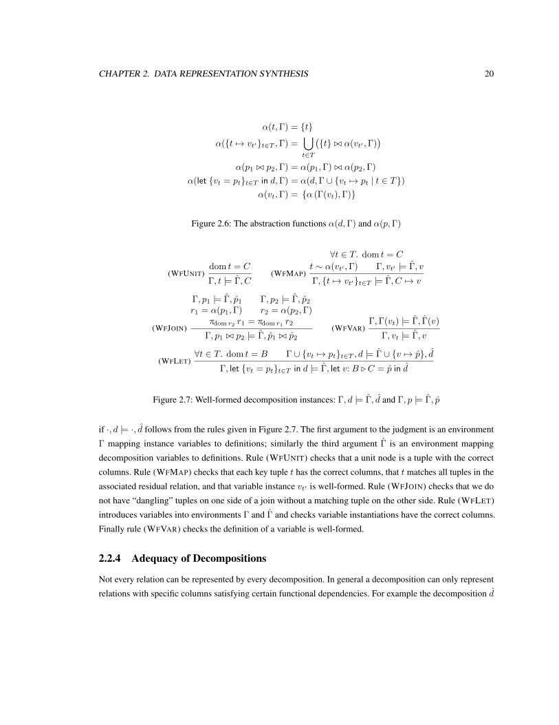
if ·, d |= ·, ˆd follows from the rules given in Figure 2.7. The first argument to the judgment is an environment� mapping instance variables to definitions; similarly the third argument ˆ
� is an environment mappingdecomposition variables to definitions. Rule (WFUNIT) checks that a unit node is a tuple with the correctcolumns. Rule (WFMAP) checks that each key tuple t has the correct columns, that t matches all tuples in theassociated residual relation, and that variable instance v
t
0 is well-formed. Rule (WFJOIN) checks that we donot have “dangling” tuples on one side of a join without a matching tuple on the other side. Rule (WFLET)introduces variables into environments � and ˆ
� and checks variable instantiations have the correct columns.Finally rule (WFVAR) checks the definition of a variable is well-formed.
2.2.4 Adequacy of Decompositions
Not every relation can be represented by every decomposition. In general a decomposition can only representrelations with specific columns satisfying certain functional dependencies. For example the decomposition ˆ
d

CHAPTER 2. DATA REPRESENTATION SYNTHESIS 21
(AVAR)(v: ; . C) 2 ⌃
⌃; ;a,�
v;C
(AUNIT)A 6= ; � `
fd
A! C
⌃;A
a,�
C;C
(AMAP)(v:A .D) 2 ⌃ � `
fd
B [ C ! A A ◆ B [ C
⌃;B
a,�
C 7! v;C [D
(AJOIN)� `
fd
A [ (B \ C)! B C ⌃;A
a,�
p
1
;B ⌃;A
a,�
p
2
;C
⌃;A
a,�
p
1
./ p
2
;B [ C
(ALET)⌃;B
a,�
p;C ⌃, v:B . C;A
a,�
ˆ
d;D
⌃;A
a,�
let v:B . C = p in
ˆ
d;D
Figure 2.8: Adequate decompositions: ⌃;Aa,�
ˆ
d;B and ⌃;A
a,�
p;B
in Figure 2.2(a) cannot represent the relation
r
0= { hns: 1, pid : 2, state:S, cpu: 42i ,
hns: 1, pid : 2, state:R, cpu: 34i},
since for each pair of ns and pid values the decomposition ˆ
d can only represent a single value for thestate and cpu fields. However r0 does not correspond to a meaningful set of processes—the relationalspecification in Section 2.1 requires that all well-formed sets of processes satisfy the functional dependencyns, pid ! state, cpu , which allows at most one state or cpu value for any given process.
We say that a decomposition ˆ
d is adequate for relations with columns C satisfying FDs � if ·; ;a,�
ˆ
d;C
follows from the rules in Figure 2.8.There are two forms of the adequacy judgement, one for decompositions: ⌃;A
a,�
ˆ
d;B, and one fordecomposition primitives: ⌃;A
a,�
p;B. The first argument to the judgement is an environment ⌃ that mapsa variable v bound in the context to a pair B . C, where B is the set of columns bound on any path to node v
from the root of the decomposition, and C is the set of columns bound within the subgraph rooted at v. Thesecond argument A is a set of columns fixed by the context. If a decomposition ˆ
d is adequate, then it canrepresent every possible relation with columns C satisfying FDs �:
Lemma 2.1 (Soundness of Adequacy). If ·; ;a,�
ˆ
d;C then for each relation r with columns C such thatr |=
fd
� there is some d such that ·, d |= ·, ˆd and ↵(d, ·) = r.
Proof. See Section 2.6.1.
The adequacy rules enforce several properties, most of which are boundary conditions. Rule (AVAR)ensures the root vertex has exactly one instance (since ; has only one valuation). Rules (AUNIT) and (AMAP)record the columns they contain, and the top-level rule (AVAR) then ensures the decomposition representsall columns of the relation. Rule (AUNIT) also ensures that unit decompositions are not part of the graph
CHAPTER 2. DATA REPRESENTATION SYNTHESIS 22
root. Since a unit decomposition represents exactly one tuple, a unit decomposition at the root (A = ;) wouldprevent us from representing the empty relation.
Rule (AMAP) is the most involved and consequential rule. Sharing occurs when the same variable is thetarget of two or more maps (see the uses of variable w in Figure 2.5(a) for an example). Rule (AMAP) checksin two steps that decomposition instances are shared only when the corresponding relations are equal. First,note that B [C are columns bound from the root to v, and the functional dependency B [C ! A guaranteesthere is a unique valuation of A per valuation of B [ C. Second, the requirement that A ◆ B [ C guaranteesthat A includes all the columns bound on all paths reaching v (since this same requirement is also appliedto other map edges that share v). Because B [ C ! A, and A includes any other key columns used in othermaps reaching v, the sub-relation reached via any of these alternative paths is the same.
To split a relation into two parts using a join decomposition, rule (AJOIN) requires a functional dependencythat ensures that we can match tuples from each side without anomalies, such as missing or spurious tuples;recall denotes symmetric difference. Finally rule (ALET) introduces variable typings from let bindings intothe variable binding environment ⌃.
2.3 Querying and Updating Decomposed Relations
In Section 2.2 we introduced decompositions, which describe how to represent a relation in memory as acollection of data structures. In this section we show how to compile the relational operations described inSection 2.1 into code tailored to a particular decomposition. There are two basic kinds of relational operation,namely queries and mutations. Since we use queries when implementing mutations, we describe queries first.
2.3.1 Queries and Query Plans
Recall that the query operation retrieves data from a relation; given a relation r, a tuple t, and a set of columnsC, a query returns the projection onto columns C of the tuples of r that match tuple t. We implement queriesin two stages: query planning, which attempts to find the most efficient execution plan q for a query, and queryexecution, which evaluates a particular query plan over a decomposition instance. This approach is well-knownin the database literature, although our formulation is novel.
In the RELC compiler, query planning is performed at compile time; the compiler generates specializedcode to evaluate the chosen plan q with no run-time planning or evaluation overhead. The compiler is freeto use any method it likes to chose a query plan, as long as the resulting query satisfies the query validitycriteria described in Section 2.3.2. We describe the query planner implementation of the RELC compiler inSection 2.3.3.
As a motivating example, suppose we want to find the set of pid values of processes that match the tuplehns: 7, state:Ri using the decomposition of Figure 2.2. That is, we want to find the running processes innamespace 7. One possible strategy would be to look up hstate:Ri on the right-hand side, and then to iterateover all ns, pid pairs associated with the state, checking to see whether they are in the correct namespace.

CHAPTER 2. DATA REPRESENTATION SYNTHESIS 23
q ::= qunit | qscan(q) | qlookup(q) | qlr(q, lr) | qjoin(q1
, q
2
, lr)
lr ::= left | right
Figure 2.9: Query plan operators
Another strategy would be to look up namespace 7 on the left-hand side, and to iterate over the set of pidvalues associated with the namespace. For each pid we then check to see whether the ns and pid pair is in theset of processes associated with hstate:Ri on the right-hand side. Each strategy has a different computationalcomplexity; the query planner enumerates the alternatives and chooses the “best” strategy.
We describe the semantics of query execution using a function dqexec q d t which takes a query plan q, adecomposition instance d, an input tuple t, and evaluates the plan over the decomposition, and produces a setof tuples in the denotation of d that match tuple t. We do not implement dqexec directly; instead the compileremits instances of dqexec specialized to particular queries q.
A query plan is a tree of query plan operators, shown in Figure 2.9. The query plan tree is superimposedon a decomposition and rooted at the decomposition’s root. A query plan prescribes an ordered sequence ofnodes and edges of the decomposition instance to visit. There are five query plan operators:
Unit The qunit operator returns the unique tuple represented by a unit decomposition instance if that tuplematches t. It returns the empty set otherwise.
Scan The operator qscan(q) invokes operator q for each child node v
s
where s matches t. Recall a mapprimitive is a mapping from a set of key columns C to a set of child nodes {v
t
}t2T
. Since operatorqscan iterates over the contents of a map data structure, it typically takes time linear in the number ofentries.
Lookup The qlookup(q) operator looks up a particular set of key values in a map decomposition; each of thekey columns of the map must be bound in the tuple t given as input to the operator. Query operator qis invoked on the resulting sub-decomposition, if any. The complexity of the qlookup depends on theparticular choice of data structure . In general, we expect qlookup to have better time complexity thanqscan.
Left/Right The qlr(q, lr) operator performs query q on either the left-hand or right-hand side of a joinspecified by the argument lr . The other side of the join is ignored.
Join The qjoin(q
1
, q
2
, lr) operator performs a join across both sides of a join decomposition. The computa-tional complexity of the join may depend on the order of evaluation. If lr is the value left, then firstquery q
1
is executed on the left side of the join decomposition, then query q
2
is executed on the rightside of the join for each tuple returned by tuple q
1
; the result of the join operator is the natural join ofthe two subqueries. If lr is the value right, the two queries are executed in the opposite order.

CHAPTER 2. DATA REPRESENTATION SYNTHESIS 24
In the scheduler example, the query
query r hns: 7, pid : 42i {cpu}
returns the cpu values associated with the process with pid 42 in namespace 7. One possible query plan is:
q
cpu
= qlr(qlookup(qlookup(qunit)), left).
To perform query q
cpu
on an instance d we evaluate
dqexec q
cpu
d hns: 7, pid : 42i
which first looks up namespace 7 in the data structure corresponding to decomposition edge from x to y,returning an instance of node y. We lookup pid 42 in the data structure corresponding to the edge from y to w,obtaining an instance of node w. We then use the qunit operator to retrieve the cpu value associated with nodew.
Recall our motivating example, namely the query
query r hns: 7, state:Ri {pid}
that returns the set of running processes in namespace 7. Two plans that implement the query are
q
1
= qjoin
�qlookup(qscan(qunit)), qlookup(qlookup(qunit)), left
�
q
2
= qlr
�qlookup(qscan(qunit)), right
�.
Plan q
1
first enumerates the set of processes with ns 7 (the left-hand side of the join), and then checks whethereach process is associated with the running state (the right-hand side of the join). Plan q
2
iterates over allprocesses in the running state, checking to see whether they are in the appropriate namespace.
An important property of the query operators is that they all require only constant space; there is noneed to construct intermediate data structures to execute a query. Having a predictable space overhead forqueries ensures that query execution does not need to allocate memory. Constant-space queries can also be adisadvantage; for example, the current restrictions would not allow a “hash-join” strategy for implementingthe join operator, nor is it possible to perform duplicate-elimination. It would be straightforward to extend thequery language with non-constant-space operators.
2.3.2 Query Validity
Not every query plan is a correct strategy for evaluating a query. We must check three properties: first thatqueries produce all of the columns requested as output, second that when performing a lookup we already

CHAPTER 2. DATA REPRESENTATION SYNTHESIS 25
(QUNIT)ˆ
�, C,A
q,�
qunit, C
(QSCAN)ˆ
�,
ˆ
�(v), (A [ C)
q,�
q,B
ˆ
�, C 7! v,A
q,�
qscan(q), B [ C
(QLOOKUP)C ✓ A
ˆ
�,
ˆ
�(v), A
q,�
q,B
ˆ
�, C 7! v,A
q,�
qlookup(q), B [ C
(QJOIN)
ˆ
�, p
1
, A
q,�
q
1
, B
1
ˆ
�, p
2
, A [B
1 q,�
q
2
, B
2
� `fd
A [B
1
! B
2
� `fd
A [B
2
! B
1
ˆ
�, p
1
./ p
2
, A
q,�
qjoin(q
1
, q
2
, left), B
1
[B
2
or ˆ�, p2
./ p
1
, A
q,�
qjoin(q
2
, q
1
, right), B
1
[B
2
(QLR)ˆ
�, p
1
, A
q,�
q,B
ˆ
�, p
1
./ p
2
, A
q,�
qlr(q, left), B or ˆ�, p2
./ p
1
, A
q,�
qlr(q, right), B
(QVAR)ˆ
�,
ˆ
�(v), A
q,�
q,B
ˆ
�, v, A
q,�
q,B
(QLET)ˆ
� [ {v 7! p}, ˆd,Aq,�
q,B
ˆ
�, let v: · · · = p in
ˆ
d,A
q,�
q,B
Figure 2.10: Valid query plans: ˆ�, ˆd,Aq,�
q,B
have all of the necessary key columns, and third that enough columns are computed on each side of a join sothat tuples from each side can be accurately matched with one another. Figure 2.10 gives inference rules for avalidity judgment that is a sufficient condition for query plan correctness. We say a query plan is valid, writtenˆ
�,
ˆ
d,A
q,�
q,B if q correctly answers queries over decomposition ˆ
d, where A is the set of columns bound inthe input tuple pattern t and B is the set of columns bound in the output tuples; ˆ� is an environment that mapsvariables in the decomposition to their definitions, whereas � is a set of FDs.
Rule (QUNIT) states that querying a unit decomposition binds its fields. Rule (QSCAN) states whenscanning over a map decomposition we bind the keys of the map both as input to the sub-query and in theoutput. Rule (QLOOKUP) is similar, however lookups require that the key columns already be bound in theinput. Rule (QJOIN) requires that each subquery of a join must bind enough columns so that we can match theresults of the two subqueries without any ambiguity. As a special case, rule (QLR) allows arbitrary queriesthat only inspect one side of a join. Finally rules (QVAR) and (QLET) handle introduction and elimination ofdecomposition variables into the variable binding environment ˆ�.
Lemma 2.2 (Decomposition Query Soundness). Suppose we have ˆ
d, C, �, d, and r such that decompositionˆ
d is adequate (i.e., ·; ;a,�
ˆ
d;C), instance d is well-formed (i.e., ·, d |= ·, ˆd), and d represents a relation r (i.e.,↵(d, ·) = r) satisfying the FDs � (i.e., � |=
fd
r). If a query plan q is valid for input tuples with columns Aand produces columns B (i.e., ·, ˆd,A
q,�
q,B), then for any tuple s with dom s = A we have
⇡
B
(dqexec q d s) = ⇡
B
{t 2 r | t ◆ s}.
Proof. See Section 2.6.2.

CHAPTER 2. DATA REPRESENTATION SYNTHESIS 26
2.3.3 Query Planner
To pick good implementations for each query, the compiler uses a query planner that finds the query plan withthe lowest cost as measured by a heuristic cost estimation function. The query planner enumerates the set ofvalid query plans for a particular decomposition d, input columns B, and output columns C, and it returns theplan with the lowest cost. It is straightforward to enumerate query plans, although there may be exponentiallymany possible plans for a query.
The RELC compiler uses a simple query cost estimator Eˆ
�
that has performed well in our experiments.Many extensions to our cost model are possible, inspired by the large literature on database query planning.For every edge from node v
1
to node v
2
in a decomposition ˆ
d we require a count c(v1
, v
2
) of the expectednumber of instances of the edge outgoing from any given instance of node v
1
. The count can be providedby the user, or recorded as part of a profiling run. Each data structure must provide a function m
(n) thatestimates the number of memory accesses to lookup a key in a data structure containing n elements. For abinary tree we might set m
btree
(n) = log
2
n, whereas for a linked list we might set mdlist
(n) = n. Let ˆ� bethe environment mapping each let-bound variable in ˆ
d to its definition. We compute Eˆ
�
(q, v,
ˆ
d), where v is thedecomposition root:
E
ˆ
�
(qunit, v, C) = 1
E
ˆ
�
(qscan(q), v
1
, C
7�! v
2
) = c(v
1
, v
2
)⇥ E
ˆ
�
(q, v
2
,
ˆ
�(v
2
))
E
ˆ
�
(qlookup(q), v
1
, C
7�! v
2
) = m
(c(v
1
, v
2
))⇥ E
ˆ
�
(q, v
2
,
ˆ
�(v
2
))
E
ˆ
�
(qjoin(q
1
, q
2
, _), v, p1
./ p
2
) = E
ˆ
�
(q
1
, v, p
1
) + E
ˆ
�
(q
2
, v, p
2
)
E
ˆ
�
(qlr(q, left), v, p
1
./ p
2
) = E
ˆ
�
(q, v, p
1
)
E
ˆ
�
(qlr(q, right), v, p
1
./ p
2
) = E
ˆ
�
(q, v, p
2
)
The cost estimate for joins is optimistic since it assumes that queries on each side of the join need only beperformed once each, whereas in general one side of a join is executed once for each tuple yielded by the otherside. We could extend the heuristic to estimate how many tuples are returned by a query, however this has notproved necessary so far.
2.3.4 Mutation: Empty and Insert Operations
Next we turn our attention to compiling the empty and insert operations. The empty operation is implementedusing a function dempty
ˆ
d which creates an empty instance of a decomposition ˆ
d. The insert operation isimplemented by a function dinsert
ˆ
d t d, which inserts a tuple t into a decomposition instance d.To create an empty instance of a decomposition, the dempty operation simply creates a single instance of
the root node of the decomposition graph; since the relation does not contain any tuples, we do not need tocreate instances of any map edges. The adequacy conditions for decompositions ensure that the root node doesnot contain any unit decompositions, so it is always possible to represent the empty relation.

CHAPTER 2. DATA REPRESENTATION SYNTHESIS 27
(a) (b)x
y
1
z
S
z
R
w
1
1
w
1
2
ns
1
S
state
R
pid
1
2
ns, pid
1, 1
ns, pid
1, 2
hcpu: 7i hcpu: 4i
x
y
1
y
2
z
S
z
R
w
1
1
w
1
2
w
2
1
ns
1
2
S
state
R
pid
1
2
pid
1
ns, pid
1, 1
2, 1
ns, pid
1, 2
hcpu: 7i hcpu: 4i hcpu: 5i
Figure 2.11: Example of insertion and removal. Inserting the tuple t = hns: 2, pid : 1, state:S, cpu: 5i intoinstance (a) produces instance (b); conversely removing tuple t from (b) produces (a). Differences between theinstances are shown using dashed lines.
To insert a tuple t into an instance d of a decomposition ˆ
d, for each node v:B . C in the decompositionwe need to find or create an instance v
s
where s = ⇡
B
t in the decomposition instance. For each edge in thedecomposition we also need to find or create an instance of the edge connecting the corresponding pair ofnode instances.
We perform insertion over the nodes of a decomposition in topologically-sorted order. For each node v
we locate the existing node instance v
s
corresponding to tuple t, if any. If no such v
s
exists, we create one,inserting v
s
into any data structures that link it to its ancestors. For example, suppose we want to insert thetuple
t = hns: 2, pid : 1, state:S, cpu: 5i
into the decomposition instance shown in Figure 2.11(a). We need to find or create the node instances xhi,yhns: 2i, zhstate:Si, and whns: 2,pid: 1,state:S,cpu: 5i. We consider each in topologically-sorted order. Node xhi isthe root of the decomposition instance, so we know its location already. Next we lookup the tuple hns: 2i inthe instance of the map from x to y associated with xhi; no such tuple exists so we create a new node yhns: 2i
and insert it into the map. Similarly we look up the tuple hstate:Si in the instance of the map from x to z
associated with node xhi to discover the existing node instance zhstate:Si. Finally, we have a choice; we caneither look up tuple hpid : 1i in the map from y to w or look up the tuple hns: 2, pid : 1i in the map from z tow; in either case we find that no such tuple exists, hence we must create a new instance of vertex w and insertit into both maps. If tuple t was a duplicate of a tuple already present in the relation then vertex w would havealready been present and we would not need to do any further work.
2.3.5 Mutation: Removal and Update Operations
We next consider the remove and update operations. We implement remove using a function dremove
ˆ
d s d,which removes tuples matching tuple s from an instance d of decomposition ˆ
d. The operation works by

CHAPTER 2. DATA REPRESENTATION SYNTHESIS 28
(a)x
y
z
w
ns
state
pid ns, pid
cpu
(b)x
y
z
w
ns
state
pid ns, pid
cpu
Figure 2.12: Two cuts of a decomposition: (a) the cut for columns {ns, pid}, and (b) the cut for columns{state}.
removing any nodes and edges from d that form part of the representation of tuples that only match s.To implement removal and update we need the notion of a cut of a decomposition. Given a tuple t with
domain C, a cut of a decomposition ˆ
d is a partition (X,Y ) of the nodes of ˆ
d into nodes yA
2 Y that can onlybe part of the representation of tuples matching t, that is, � `
fd
A! C, and nodes xB
2 X that may formpart of the representation of tuples that do not match t, that is � `
fd
B 9 C. Figure 2.12 shows two possiblecuts of the scheduler decomposition for different sets of columns C.
Edges in a decomposition cut (X,Y ) may point from X to Y but not vice-versa. This result follows fromthe adequacy judgment, which ensures that the columns bound in the child of a map edge must functionallydetermine the columns bound in its parent. The adequacy judgement also guarantees that the cut for a particulardecomposition ˆ
d and set of columns C always exists and is unique.To remove tuples matching a tuple t using a cut (X,Y ), we simply break any edges crossing the cut. That
is, we remove any references from data structures linking instances of nodes in X to instances of nodes in Y
that form part of the representation of tuples that match t. Once all such references are removed, the instancesof nodes in Y are unreachable from the root of the decomposition instance and can be deallocated. We canalso clean up any map nodes in X that are now devoid of children.
For example, suppose we want to remove all tuples matching the tuple t = hns: 2, pid : 1i from thedecomposition instance shown in Figure 2.11(b). Tuple t has the domain C = {ns, pid}; Figure 2.12(a)shows the corresponding decomposition cut. Nodes x, y, and z lie above the cut; an instance of node x isalways present in every possible relation, instances of node y are specific to a particular namespace but notto any particular process id, and instances of node z are specific to a particular process state but not to anyparticular process. Node w lies below the cut; each instance of node w forms part of exactly one valuation forthe columns C. To perform removal, we break any instances of the edges from instances of nodes y and z toinstances of node w which match tuple t; these edges are drawn as dashed lines in Figure 2.11(b). Once thedashed edges/nodes in Figure 2.11 are removed, we have the option to deallocate the map at node y
2
as well.Our implementation deallocates empty maps to minimize space consumption.
To find the edge instances to break we can reuse the query planner. Any query that takes columns C as

CHAPTER 2. DATA REPRESENTATION SYNTHESIS 29
input and visits each of the edges we want to cut will work. One such plan is
qjoin
�qlookup(qlookup(qunit)), qlookup(qlookup(qunit)), left
�.
For some data structures, such as intrusive doubly-linked lists, we can remove edges given the destination nodealone. If the edge from z to w uses such a data structure we could use the cheaper plan:
qlr
�qlookup(qlookup(qunit)), left
�.
We implement update using a function dupdate
ˆ
d s u d, which updates tuples matching s using valuesfrom u in an instance d of decomposition ˆ
d. Semantically, updates are a removal followed by an insertion. Inthe implementation we can reuse the nodes and edges discarded in the removal in the subsequent insertion—i.e.,we can perform the update in place.
We provide only the common case for updates of tuples t matching a tuple pattern s, namely when s is akey for the relation and u does not alter columns appearing in s. Non-key patterns or key-modifying tupleupdates may merge multiple tuples, and hence require the implementation to merge nodes. Our restrictionguarantees no merging can occur. We can reuse nodes and edges below the cut, and any changes in u thatapply to nodes below the cut can be performed in-place.
2.3.6 Soundness of Relational Operations
Next we show that the operations on decompositions faithfully implement the corresponding relationalspecifications. We show that sequences of relational operations on graph decompositions are sound withrespect to their logical counterparts (Theorem 2.5) by induction using initialization and preservation lemmas.
Lemma 2.3 (Decomposition Initialization). For any decomposition ˆ
d, if d = dempty
ˆ
d then ·, d |= ·, ˆd and↵(d, ·) = ;.
Proof. See Section 2.6.3.
Lemma 2.4 (Decomposition Preservation). For all ˆ
d, �, t, d, C, and r where decomposition ˆ
d is adequate(·; ;
a,�
ˆ
d;C), decomposition instance d is well-formed (·, d |= ·, ˆd), and d represents relation r (↵(d, ·) = r)satisfying FDs � (� |=
fd
r), we have:
(a) If dom t = C, d0 = dinsert
ˆ
d t d, and � |=fd
r [ {t} then ·, d0 |= ·, ˆd and ↵(d0, ·) = r [ {t}.
(b) If dom t ✓ C and d
0= dremove
ˆ
d s d then ·, d0 |= ·, ˆd and ↵(d0, ·) = r
0 where r0 = r \ {t 2 r | t ◆ s}and r
0 |=fd
�.
(c) Suppose s is a key for r (� `fd
dom s! domC), the domains of s and u do not intersect (dom s \domu = ;), and we have d
0= dupdate
ˆ
d s u d and r
0= {if t ◆ s then t 2 u else t | t 2 r}. If
r
0 |=fd
� then ·, d0 |= ·, ˆd and ↵(d0, ·) = r
0.
Proof. See Section 2.6.3.

CHAPTER 2. DATA REPRESENTATION SYNTHESIS 30
Theorem 2.5 (Decomposition Soundness). Let C be a set of columns, � a set of FDs, and ˆ
d a decompositionadequate for C and �. Suppose a sequence of insert, update and remove operators starting from the emptyrelation produce a relation r, and that each operation satisfies the conditions of Lemma 2.4. Then the corre-sponding sequence of dinsert, dupdate, and dremove operators given dempty
ˆ
d as input produce d such that·, d |= ·, ˆd and ↵(d, ·) = r.
Proof. Follows immediately from Lemma 2.3 and Lemma 2.4 by induction.
2.4 Autotuner
Thus far we have concentrated on the problem of compiling relational operations for a particular decompositionof a relation. However, a programmer may not know, or may not want to invest time in finding the best possibledecomposition for a relation. We have therefore constructed an autotuner that, given a program written to therelational interface, attempts to infer the best possible decomposition for that program.
The autotuner takes as input a benchmark program that produces as output a cost value (e.g., execution time),together with the name of a relation to optimize. The autotuner then exhaustively constructs all decompositionsfor that relation up to a given bound on the number of edges, recompiles and runs the benchmark programfor each decomposition, and returns a list of decompositions sorted by increasing cost. We do not make anyassumptions about the cost metric—any value of interest such as execution time or memory consumption maybe used.
2.5 Experiments
We have implemented a compiler, named RELC, that takes as input a relational specification and a decom-position, and emits C++ code implementing the relation. We evaluate our compiler using micro-benchmarksand three real-world systems. The micro-benchmarks (Section 2.5.1) show that different decompositionshave dramatically different performance characteristics. Since our compiler generates C++ code, it is easyto incorporate synthesized data representations into existing systems. We apply synthesis to three existingsystems (Section 2.5.2), namely a web server, a network flow accounting daemon, and a map viewer, andshow that synthesis leads to code that is simultaneously simpler, correct by construction, and comparable inperformance to the code it replaces.
We chose C++ because it allows low-level control over memory-layout, has a powerful template system, andhas widely-used libraries of data structures from which we can draw. Data structure primitives are implementedas C++ template classes that implement a common associative container API. The set of data structures caneasily be extended by writing additional templates and providing the compiler some basic information aboutthe data structure’s capabilities. We have implemented a library of data structures that wrap code from the C++Standard Template Library and the Boost Library [Boost], namely both non-intrusive and intrusive doubly-linked lists (std::list, boost::intrusive::list), non-intrusive and intrusive binary trees (std::map,

CHAPTER 2. DATA REPRESENTATION SYNTHESIS 31
edges::relation graph_edges;nodes::relation visited;
// Code to populate graph_edges elided.
stack<int> stk;stk.push(v0);while (!stk.empty()) {int v = stk.top();stk.pop();if (!visited.query(nodes::tuple_id(v))) {visited.insert(nodes::tuple_id(v));edges::query_iterator_src__dst_weight it;graph_edges.query(edges::tuple_src(v), it);while (!it.finished()) {stk.push(it.output.f_dst());it.next();
}}
}
Figure 2.13: Depth-first search algorithm
boost::intrusive::set), hash-tables (boost::unordered_map), and vectors (std::vector). Since theC++ compiler expands templates, the time and space overheads introduced by the wrappers is minimal.
2.5.1 Microbenchmarks
We implemented a selection of small benchmarks: a benchmark based on our running example of a processscheduler, a cache benchmark based on the real systems discussed in the next section, and a graph benchmark.In this chapter, we focus just on the graph benchmark.
The graph benchmark reads in a directed weighted graph from a text file and measures the times toconstruct the edge relation, to perform forwards and backwards depth-first searches over the whole graph, andto remove each edge one-by-one. We represent the edges of a directed graph as a relation edges with columns{src, dst ,weight} and a functional dependency src, dst ! weight . We represent the set of the graph nodes asa relation nodes consisting of a single id column. The RELC compiler emits a C++ module that implementsclasses nodes::relation and edges::relation with methods corresponding to each relational operation.A typical client of the relational interface is the algorithm to perform a depth-first search, shown in Figure 2.13.The code makes use of the standard STL stack class in addition to an instance of the nodes relation visitedand an instance of the edges relation graph_edges.
To demonstrate the tradeoffs involved in the choice of decomposition, we used the autotuner framework toevaluate three variants of the graph benchmark under different decompositions. We used a single input graph
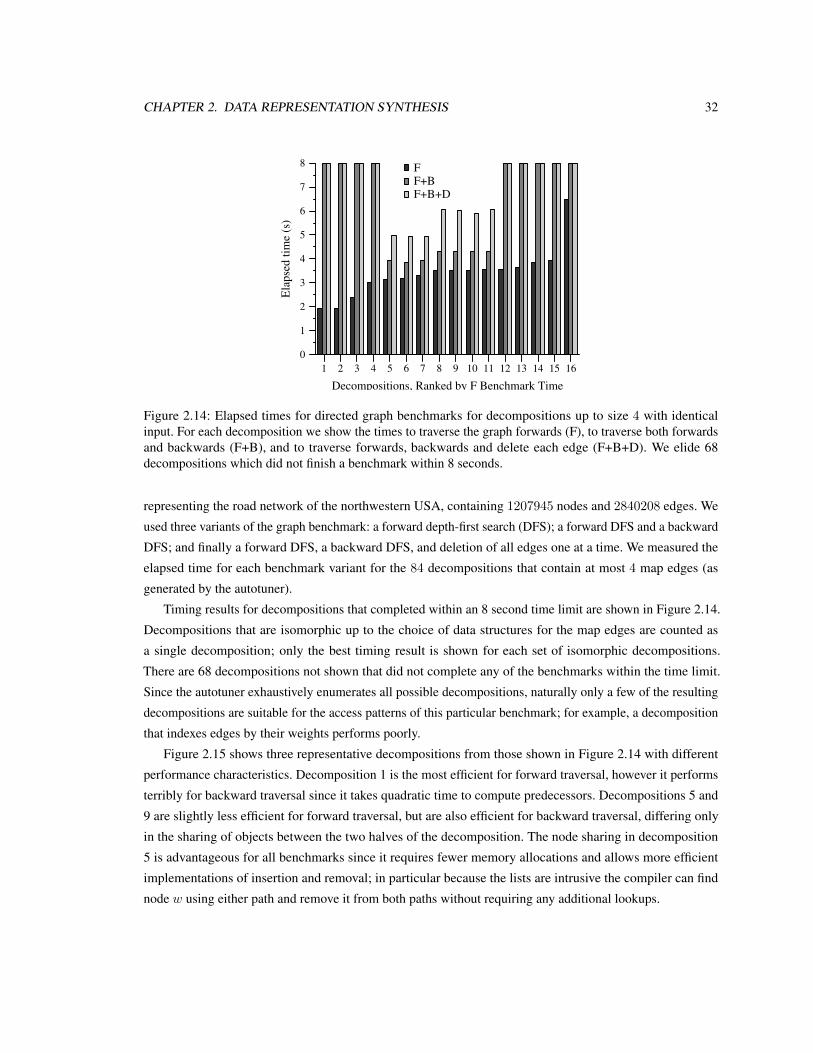
CHAPTER 2. DATA REPRESENTATION SYNTHESIS 32
1 2 3 4 5 6 7 8 9 10 11 12 13 14 15 16
Decompositions, Ranked by F Benchmark Time
0
1
2
3
4
5
6
7
8
Ela
pse
d t
ime
(s)
FF+BF+B+D
Figure 2.14: Elapsed times for directed graph benchmarks for decompositions up to size 4 with identicalinput. For each decomposition we show the times to traverse the graph forwards (F), to traverse both forwardsand backwards (F+B), and to traverse forwards, backwards and delete each edge (F+B+D). We elide 68decompositions which did not finish a benchmark within 8 seconds.
representing the road network of the northwestern USA, containing 1207945 nodes and 2840208 edges. Weused three variants of the graph benchmark: a forward depth-first search (DFS); a forward DFS and a backwardDFS; and finally a forward DFS, a backward DFS, and deletion of all edges one at a time. We measured theelapsed time for each benchmark variant for the 84 decompositions that contain at most 4 map edges (asgenerated by the autotuner).
Timing results for decompositions that completed within an 8 second time limit are shown in Figure 2.14.Decompositions that are isomorphic up to the choice of data structures for the map edges are counted asa single decomposition; only the best timing result is shown for each set of isomorphic decompositions.There are 68 decompositions not shown that did not complete any of the benchmarks within the time limit.Since the autotuner exhaustively enumerates all possible decompositions, naturally only a few of the resultingdecompositions are suitable for the access patterns of this particular benchmark; for example, a decompositionthat indexes edges by their weights performs poorly.
Figure 2.15 shows three representative decompositions from those shown in Figure 2.14 with differentperformance characteristics. Decomposition 1 is the most efficient for forward traversal, however it performsterribly for backward traversal since it takes quadratic time to compute predecessors. Decompositions 5 and9 are slightly less efficient for forward traversal, but are also efficient for backward traversal, differing onlyin the sharing of objects between the two halves of the decomposition. The node sharing in decomposition5 is advantageous for all benchmarks since it requires fewer memory allocations and allows more efficientimplementations of insertion and removal; in particular because the lists are intrusive the compiler can findnode w using either path and remove it from both paths without requiring any additional lookups.

CHAPTER 2. DATA REPRESENTATION SYNTHESIS 33
(1) (5) (9)x
y
z
src
dst
weight
x
y
z
w
src
dst
dst
src
weight
x
y
z
l
r
src
dst
dst
src
weight weight
Figure 2.15: Decompositions 1, 5 and 9 from Figure 2.14. Solid edges represent instances of the map classfrom boost::intrusive, whereas dotted edges represent instances of boost::intrusive::list.
Original SynthesisSystem Everything Module Decomposition Modulethttpd 7050 402 42 239Ipcap 2138 899 55 794ZTopo 5113 1083 39 1048
Table 2.1: Non-comment lines of code for existing system experiments. For each system, we report the sizeof entire original system and just the source module we altered, together with the size of the altered sourcemodule and the mapping file when using synthesis.
2.5.2 Data Representation Synthesis in Existing Systems
To demonstrate the practicality of our approach, we took three existing open-source systems—thttpd, Ipcap,and ZTopo—and replaced core data structures with relations synthesized by RELC. All are publicly-availableprograms with real-world users.
The thttpd web server is a small and efficient web server implemented in C. We reimplemented the moduleof thttpd that caches the results of the mmap() system call. When thttpd receives a request for a file, it checksthe cache to see whether the same file has previously been mapped into memory. If a cache entry exists, itreuses the existing mapping; otherwise it creates a new mapping. If the cache is full then the code traversesthrough the mappings removing those older than a certain threshold. Other researchers have used thttpd’scache module as a program analysis target [McCloskey et al., 2011].
The IpCap daemon is a TCP/IP network flow accounting system implemented in C. IpCap runs on anetwork gateway, and counts the number of bytes incoming and outgoing from hosts on the local network,producing a list of network flows for accounting purposes. For each network packet, the daemon looks up theflow in a table, and either creates a new entry or increments the byte counts for an existing entry. The daemonperiodically iterates over the collection of flows and outputs the accumulated flow statistics to a log file; flowsthat have been written to disk are removed from memory. We replaced the core packet statistics data structureswith relations implemented using RELC.
ZTopo is a topographic map viewer implemented in C++. A map consists of millions of small image tiles,

CHAPTER 2. DATA REPRESENTATION SYNTHESIS 34
0 5 10 15 20 25
Decompositions, Ranked by Time
0
2
4
6
8
10
12
14
Ela
pse
d T
ime
(s)
Figure 2.16: Elapsed time for IpCap to log 3 ⇥ 10
5 random packets for 26 decompositions up to size 4generated by the auto-tuner, ranked by elapsed time. The 58 decompositions not shown did not completewithin 30 seconds.
retrieved using HTTP over the internet and reassembled into a seamless image. To minimize network traffic,the viewer maintains memory and disk caches of recently viewed map tiles. When retrieving a tile, ZTopofirst attempts to locate it in memory, then on disk, and as a last resort over the network. The tile cache wasoriginally implemented as a hash table, together with a series of linked lists of tiles for each state to enablecache eviction. We replaced the tile cache data structure with a relation implemented using RELC.
Table 2.1 shows non-comment lines of code for each test-case. In each case the synthesized code iscomparable to or shorter than the original code in size. Both the thttpd and ipcap benchmarks originally usedopen-coded C data structures, accounting for a large fraction of the decrease in line count. ZTopo originallyused C++ STL and Boost data structures, so the synthesized abstraction does not greatly alter the line count.The ZTopo benchmark originally contained a series of fairly subtle dynamic assertions that verified that thetwo different representations of a tile’s state were in agreement; in the synthesized version the compilerautomatically guarantees these invariants, so the assertions were removed.
For each system, the relational and non-relational versions had equivalent performance. If the choice ofdata representation is good enough, data structure manipulations are not the limiting factor for these particularsystems. The assumption that the implementations are good enough is important, however; the auto-tunerconsidered plausible data representations that would have resulted in significant slow-downs, but foundalternatives where the data manipulation was no longer the bottleneck. For example we used the autotuneron the Ipcap benchmark to generate all decompositions up to size 4; Figure 2.16 shows the elapsed timefor each decomposition on an identical random distribution of input packets. The best decomposition is abinary-tree mapping local hosts to hash-tables of foreign hosts, which performs approximately 5⇥ fasterthan the decomposition ranked 18th, in which the data structures are identical but local and foreign hosts aretransposed. For this input distribution the best decomposition performs identically to the original hand-codedimplementation to within the margin of measurement error.
Our experiments show that different choices of decomposition lead to significant changes in performance(Section 2.5.1), and that the best performance is comparable to existing hand-written implementations (Sec-tion 2.5.2). The resulting code is concise (Sections 2.5.1 and 2.5.2), and the soundness of the compiler

CHAPTER 2. DATA REPRESENTATION SYNTHESIS 35
(Theorem 2.5) guarantees that the resulting data structures are correct by construction.
2.6 Proofs of Theorems
To minimize notational overhead, in proofs we work with decompositions and instances encoded via envi-ronments rather than let-bindings. We represent a decomposition ˆ
d as a pair of the environment ˆ� and a rootvariable z (as constructed by the well-formedness rules). If a decomposition is adequate then there exists anadequacy type environment ⌃ (as constructed by the adequacy inference rules) such that for each v 2 dom�
we have ⌃(v) = A . B and ⌃;A
a,�
ˆ
�(v);B holds; further we must have ⌃(z) = ; . C for some C;we say the decomposition is adequate for C and �. We preserve the order of the original let-bindings viaa total variable order �, which is a reverse topological sort of the decomposition graph. As in the case ofdecompositions, we represent an instance as a pair of an environment � and a root variable vhi.
2.6.1 Soundness of Adequacy
We prove a strengthened version of Lemma 2.1 by induction; Lemma 2.1 then follows as a special case.
Lemma 2.6. Suppose we have an adequate decomposition ˆ
d, represented by ˆ
�, v, and ⌃, where ⌃(z) = ; .Z.Then for any relation r such that dom r = Z and r |=
fd
�, there exists an environment � such that for allv where ˆ
�(v) = p and ⌃(v) = X . Y and any t 2 ⇡X
r we have �(v
t
) = p
t
such that �, pt
|= ˆ
�, p and↵(p
t
,�) = ⇡
Y
�
t
r.
Proof. By induction on the let binding order. The base case is trivial. Suppose there exists v such that thehypothesis holds for all w � v. We must have ⌃(v) = X . Y and ⌃;X
a,�
ˆ
�(v);Y since the decompositionis adequate. We now prove the existence of each p
t
instance by another induction on the derivation of theadequacy judgement.
If the outermost rule is (AUNIT) we must have p = C and � `fd
X ! Y . For any t 2 ⇡
X
r set�(v
t
) = p
t
= ⇡
Y
�
t
r; we are guaranteed the right-hand side of the expression is a single tuple by thefunctional dependency. We have �, p
t
|= ˆ
�, Y immediately by WFUNIT, and we have ↵(pt
,�) = ⇡
Y
�
t
r bythe definition of the abstraction function.
If the outermost rule is (AMAP), then we have p = C 7! v
0, and there exists A, B, C, D such that X = B,Y = C [D, ⌃(v0) = A .D, � `
fd
B [ C ! A and A ◆ B [ C. For any t 2 ⇡B
r we set
�(v
t
) = p
t
= {t 7! v
0t
0 | t 2 ⇡C
�
u
r, ⇡
A
�
t
�
u
r = {t0}}.
Well-formedness �, pt
|= ˆ
�, p follows from (WFMAP), and the induction hypothesis. For ↵(pt
,�), note that

CHAPTER 2. DATA REPRESENTATION SYNTHESIS 36
⇡
A
�
t
�
u
r = {t0} since r |=fd
� and � `fd
B [ C ! A by assumption. Hence we have:
↵(p
t
,�) =
[
t2⇡C �u r
{t} ./ ↵(vt
0,�)
=
[
t2⇡C �u r
{t} ./ ⇡D
(r ./ ⇡
A
�
t
�
u
r)
=
[
t2⇡C �u r
{t} ./ ⇡D
(r ./ ⇡
A
�
t
�
u
r)
=
[
t2⇡C �u r
{t} ./ ⇡D
�
t
�
u
(r ./ ⇡
A
r)
=
[
t2⇡C �u r
{t} ./ ⇡D
�
t
�
u
r = ⇡
C[D
�
u
r
If the outermost rule is (AJOIN), then we have X = A, Y = B [ C, p = p
1
./ p
2
, and by the IH wehave p
1
and p
2
such that �, p1
|= p
1
,, �, p2
|= p
2
,, ↵(p1
,�) = ⇡
B
�
u
r, and ↵(p2
,�) = ⇡
C
�
u
r. Observe�, p
1
./ p
2
|= p
1
./ p
2
, follows from rule (WFJOIN), and we have
↵(p
1
./ p
2
,�) = ⇡
B
�
u
r ./ ⇡
C
�
u
r = ⇡
(B[C)
�
u
r
by the definition of the abstraction function and the functional dependency hypothesis of the rule.
We now have:
Proof of Lemma 2.1. Follows from Lemma 2.6.
2.6.2 Soundness of Queries
To prove Lemma 2.2 we define a variant dqexec formally. We then show a strengthened version of Lemma 2.2by induction, and the result follows.
We define dqexec q � p s:
dqexec qunit � t s = if s ⇠ t then {t} else ;dqexec qscan(q) � {t 7! v
t
0}t2T
s =
S{t ./ dqexec q � �(v
t
0) s
0 | t 2 T, s
0 2 s ./ t}dqexec qlookup(q) � {t 7! v
t
0}t2T
s =
S{t ./ dqexec q � �(v
t
0) s | t 2 T, s = t}
dqexec qlr(q
1
, q
2
, left) � (p
1
./ p
2
) s = dqexec q
1
� p
1
s
dqexec qlr(q
2
, q
1
, right) � (p
2
./ p
1
) s = dqexec q
2
� p
2
s
dqexec qjoin(q
1
, q
1
, left) � (p
1
./ p
2
) s = dqexec qjoin(q
2
, q
1
, right) � (p
2
./ p
1
) s =
S{(dqexec q
2
� p
2
s
0) ./ t | t 2 dqexec q
1
� p
1
s, s
0 2 s ./ t}
Note that we write a pair of an environment � and p in place of a decomposition d.We write �/C to denote the set of FDs �0 where instances of columns C are constant and hence have
been removed from both the right-hand and left-hand side of all FDs in �.

CHAPTER 2. DATA REPRESENTATION SYNTHESIS 37
Lemma 2.7. Suppose we have �, p, ˆ�, p, and ⌃, such that p is adequate (⌃;Fa,�
p;G for some F and G),p is well-formed (�, p |= ˆ
�, p), and the denotation of p satisfies FDs �/A (↵(p,�) |=fd
�/A). If q is a validquery (ˆ�, p, A
q,�
q,B) and s a tuple with dom s = A we have
dqexec q � p s = ⇡
B
�
s
↵(p,�).
Proof. By induction on the derivation of ˆ�, p, Cq,�
q,D.If the outermost rule is (QUNIT), then we have q = qunit, p = B, and we must have p = t where
dom t = B by well-formedness. Then
dqexec qunit � t s
= if s ⇠ t then {t} else ;
= ⇡
B
�
s
t
= ⇡
B
�
s
↵(t,�).
If the outermost rule is (QSCAN) then we have q = qscan(q
0), p = C 7! v, and we must have d = {t 7!
v
t
0}t2T
by well-formedness. Now
dqexec qscan(q
0) � {t 7! v
t
0}t2T
s
=
[{t ./ dqexec q0 � �(v
t
0) s
0 | t 2 T, s
0 2 s ./ t}
=
[{t ./ ⇡
B
�
s
0↵(v
t
0,�) | t 2 T, s
0 2 s ./ t}
follows by the induction hypothesis
= ⇡
B[C
�
s
[{t ./ ↵(v
t
0,�) | t 2 T}
= ⇡
B[C
�
s
↵({t 7! v
t
0}t2T
,�).
Rule (QLOOKUP) is a special case of rule (QSCAN).If the outermost rule is (QLR) say we have q = qlr(q
1
, left), p = p
1
./ p
2
and p = p
1
./ p
2
. Then
dqexec qlr(q
1
, left) � p
1
./ p
2
s
= dqexec q
1
� p
1
s
= ⇡
B
�
s
↵(p
1
,�)

CHAPTER 2. DATA REPRESENTATION SYNTHESIS 38
follows by the induction hypothesis, and
= ⇡
B
�
s
(↵(p
1
,�) ./ ↵(p
2
,�))
follows by well-formedness, finally
= ⇡
B
�
s
↵(p
1
./ p
2
,�).
The right case follows by symmetry.If the outermost rule is (QJOIN) assume without loss of generality we have q = qjoin(q
1
, q
2
, left),p = p
1
./ p
2
and p = p
1
./ p
2
; the qright case follows by symmetry. Now,
dqexec qjoin(q
1
, q
2
, left) � p
1
./ p
2
s
=
[{(dqexec q
2
� p
2
s
0) ./ t | t 2 dqexec q
1
� p
1
s, s
0 2 s ./ t}
and by the induction hypothesis
=
[{(⇡
B2 �s0↵(p
2
,�)) ./ t | t 2 ⇡B1 �s ↵(p1,�), s
0 2 s ./ t}
By adequacy and the hypotheses we have
= (⇡
B2 �s ↵(p2,�)) ./ (⇡B1 �s ↵(p1,�))
= ⇡
B1[B2 �s(↵(p2,�) ./ ↵(p1,�))
= ⇡
B1[B2 �s ↵(p1 ./ p2,�).
Proof of Lemma 2.2. Follows from Lemma 2.7.
2.6.3 Soundness of Mutations
Empty
Formally we define dempty on let-free decompositions.Suppose we have an adequate decomposition ˆ
d represented by ˆ
�, z, ⌃. Then we define
dempty
ˆ
�,z
() = {zhi 7! emp
ˆ
�(z)},

CHAPTER 2. DATA REPRESENTATION SYNTHESIS 39
where
emp (C 7! v) = {}
emp p
1
./ p
2
= (emp p
1
./ emp p
2
)
There is no case for unit decompositions; a unit decomposition cannot represent an empty relation and theadequacy conditions guarantee that none is necessary.
Proof of Lemma 2.3. Follows from the definition of dempty and the definitions of well-formedness and theabstraction.
Insert
To define insertion we define auxiliary functions singleton⌃
, which creates a singleton primitive instance, andadd
⌃
, which inserts a tuple into an existing primitive instance. Each function operates over a decompositionwith typing ⌃. We define:
singleton
⌃
C t = ⇡
C
t
singleton
⌃
(C 7! v) t = {⇡C
t 7! v
u
} where v:A .B 2 ⌃ and u = ⇡
A
t
singleton
⌃
(p
1
./ p
2
) t = singleton
⌃
p
1
t ./ singleton
⌃
p
2
t
and
add
⌃
C t u = t when ⇡
C
u = t
add
⌃
(C 7! v) {t 7! v
t
0}t2T
u = {t 7! v
t
0}t2T
[ {⇡C
u 7! v
u
0} where v:A .B 2 ⌃ and u
0= ⇡
A
u
add
⌃
(p
1
./ p
2
) (p
1
./ p
2
) t = add
⌃
p
1
p
1
t ./ add
⌃
p
2
p
2
t
Now we can define insertion dinsert
ˆ
�,z,⌃
u � = �
0, where for any (v:A .B) 2 ⌃ we define
�
0(v
t
) =
8>>>>>><
>>>>>>:
�(v
t
) if vt
2 dom�, t 6= ⇡
A
u
add
⌃
ˆ
�(v) v
t
u if vt
2 dom�, t = ⇡
A
u
singleton
⌃
ˆ
�(v) u if vt
/2 dom�, t = ⇡
A
u
undefined otherwise
Lemma 2.8. Suppose we have a decomposition ˆ
d adequate for Z and �, represented by ˆ
�, z, and ⌃, and let �be a well-formed instance. Let r = ↵(zhi,�), let u be a tuple with domu = Z, let r0 = r [ {u}, and supposer
0 |=fd
�. Suppose dinsertˆ
�,z,⌃
u � = �
0. For all (v:A .B) 2 ⌃ and all vt
2 �
0 let p =
ˆ
�(v), let pt
= �(v
t
)

CHAPTER 2. DATA REPRESENTATION SYNTHESIS 40
if defined, and let p0t
= �
0(v
t
). Then �
0, p
0t
|= ˆ
�, p and
↵(p
0t
,�
0) =
8<
:↵(p
t
,�) [ ⇡dom p
�
t
{u} if vt
2 dom�
⇡
dom p
�
t
{u} otherwise.
Proof. By induction on let-binding order. The base case is trivial. Take some (v:A .B) 2 ⌃ and suppose theresult holds for all w where w � v. There are three cases:
If vt
2 dom� and t 6= ⇡
A
u, the adequacy result ensures that all children v
0t
0 of node v
t
have t
0 ◆ t, andare not modified by the insertion. The well-formedness and abstraction results follow immediately by inductionon the structure of �(v
t
).If v
t
2 dom� and t = ⇡
A
u then we have p
t
= add
⌃
ˆ
�(v) �(v
t
) u. We show the result by induction onthe structure of p:
• If p = C then we have p
t
= u
0 where � `fd
dom t! C and r
0 |=fd
�, so we must have ⇡C
u = u
0=
p
0t
. Well-formedness and abstraction then follow from the definitions.
• If p = C 7! v
0 then we have p
t
= {s 7! v
0s
0}s2S
and p
0t
= {s 7! v
0s
0}s2S
[ {⇡C
u 7! v
0u
0} where⌃(v
0) = D . E and u
0= ⇡
D
u. The result then follows from the (outer) induction hypothesis and thedefinitions of well-formedness and abstraction.
• If p = p
1
./ p
2
then we have p
t
= p
1
./ p
2
and the result follows easily by the induction hypothesisand the definitions.
If vt
/2 dom� and t = ⇡
A
u then we have �
0(v
t
) = singleton
⌃
ˆ
�(v) u. We show the result by inductionon the structure of p, where we take ↵(p
t
,�) to be empty in
• If p = C the result follows from the definitions.
• If p = C 7! v
0 the result follows from the outer induction hypothesis and the definitions.
• If p = p
1
./ p
2
the result follows from the inner induction hypothesis and the definitions.
Remove
To define removal of tuples matching s where dom s = Z in a decomposition, recall a decomposition cut(X,Y ) is a partition of the nodes (v: A . B) 2 ⌃, that is, we have � `
fd
A 9 Z for all v 2 X and� `
fd
A! Z for all v 2 Y .

CHAPTER 2. DATA REPRESENTATION SYNTHESIS 41
We define an auxiliary function del p p V :
del C t V = t
del (C 7! v) {t 7! v
t
0}t2T
V = {t 7! v
t
0 | t 2 T, v
t
0/2 V }
del (p
1
./ p
2
) (p
1
./ p
2
) V = del p
1
p
1
V ./ del
⌃
p
2
p
2
V
Suppose we have an instance defined by (�, whi), where ↵(whi,�) = r. Let s be a tuple. We definer
0= {t 2 r | t + s} and
V = {vt
| vt
2 dom�, v 2 Y, ⌃(v) = A .B, t /2 ⇡A
�
s
r
0}.
We then define dremove
ˆ
�,z,⌃
s � = �
0, where for any (v:A .B) 2 ⌃
�
0(v
t
) =
8>>><
>>>:
del
ˆ
�(v) �(v
t
) V if v 2 X, v
t
2 dom�
�(v
t
) if v 2 Y, v
t
2 dom� \ V
undefined otherwise
In the definition of removal given here the set of nodes to prune V is computed in advance, and then pruned.Since we want a constant-space implementation, in practice we interleave the computation of V with pruning.
Lemma 2.9. Suppose we have an adequate decomposition ˆ
d, represented by ˆ
�, v, and ⌃, and suppose thatdremove
ˆ
�,z,⌃
u � = �
0. Then for all (v: A . B) 2 ⌃ and all vt
2 �
0, let p =
ˆ
�(v), let pt
= �(v
t
), and letp
0t
= �
0(v
t
). We have �, p
t
|= ˆ
�, p and
↵(p
0t
,�
0) = ↵(p
t
,�) \ ⇡dom p
�
t
{s 2 r | s ◆ u}.
Proof. By induction on let-binding order. The base case is trivial. Take some (v:A .B) 2 ⌃ and suppose theresult holds for all w where w � v. There are two cases: If v 2 Y and v
t
2 dom� \ V then by the adequacyjudgement all descendants v0
t
0 of vt
have t0 ◆ t and hence cannot be in V . The well-formedness and abstractionresults are immediate.
If v 2 X and v
t
2 dom� then the result follows by induction on the structure of p:
• If p = C the result is immediate.
• If p = C 7! v
0 the result follows from the outer induction hypothesis and the definitions.
• If p = p
1
./ p
2
then the result follows from the inner induction hypothesis and the definitions.
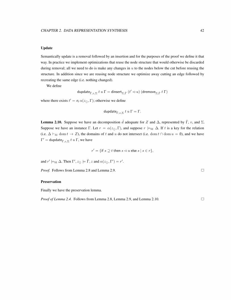
CHAPTER 2. DATA REPRESENTATION SYNTHESIS 42
Update
Semantically update is a removal followed by an insertion and for the purposes of the proof we define it thatway. In practice we implement optimizations that reuse the node structure that would otherwise be discardedduring removal; all we need to do is make any changes in u to the nodes below the cut before reusing thestructure. In addition since we are reusing node structure we optimize away cutting an edge followed byrecreating the same edge (i.e. nothing changed).
We definedupdate
ˆ
�,z,⌃
t u � = dinsert
⌃,
ˆ
�
(t
0 2 u) (dremove
⌃,
ˆ
�
t �)
where there exists t0 = �
t
↵(zhi,�); otherwise we define
dupdate
ˆ
�,z,⌃
t u � = �.
Lemma 2.10. Suppose we have an decomposition ˆ
d adequate for Z and �, represented by ˆ
�, v, and ⌃.Suppose we have an instance �. Let r = ↵(zhi,�), and suppose r |=
fd
�. If t is a key for the relation(i.e. � `
fd
dom t ! Z), the domains of t and u do not intersect (i.e. dom t \ domu = ;), and we have�
0= dupdate
ˆ
�,z,⌃
t u �, we have
r
0= {if s ◆ t then s 2 u else s | s 2 r},
and r
0 |=fd
�. Then �
0, zhi |= ˆ
�, z and ↵(zhi,�0) = r
0.
Proof. Follows from Lemma 2.8 and Lemma 2.9.
Preservation
Finally we have the preservation lemma.
Proof of Lemma 2.4. Follows from Lemma 2.8, Lemma 2.9, and Lemma 2.10.

Chapter 3
Lock Placements
In Chapter 2, we introduced data representation synthesis, a technique for synthesizing low-level representationsof data from a high-level relational description. Next, we consider the problem of extending our synthesisapproach to generate data representations that support concurrent access from multiple threads. Before we cando so, in this chapter we first develop the theory of lock placements, which describe the mapping betweenlocks and the data they protect, and which form an important building block for concurrent data representationsynthesis (Chapter 4).
Most concurrent software uses locks as a primitive for ensuring mutual exclusion between threads. Whileit is correct to say that the key characteristic of a lock is that it may be held by only one thread at a time, such adescription fails to capture the higher-level purposes for which programmers use locks. Universally, locks areused to protect data, guaranteeing that only one thread operates on particular parts of the store at a time. Theassociation between locks and the data they protect is, however, implicit, and in the presence of mutable datastructures it is not even clear how to describe the relationship between a possibly changing set of locks and thechanging heap the locks protect.
This chapter investigates what it means for locks to protect data. So far as we are aware, there are noproposals in the literature for even stating the relationship between locks and the data they protect in a way thatcaptures the range of ways in which locks are used in practice. In particular, we are interested in explainingspeculative locks and the common case in which updates to the heap change which data locks protect. Webelieve ours is the first proposal to address these issues.
To explain our results, we begin with a slightly informal, simple, obviously correct, but impractical lockingprotocol. We assume the heap consists of a graph of objects (nodes), each of which has a set of fields (edges)that point to other objects. We also assume that concurrent operations are expressed as transactions that executeatomically (e.g., atomic blocks). Every heap edge has a logical lock. Each transaction t must obey a standardtwo-phase locking protocol:
1. Acquire all logical locks of every edge read or written by t.
43

CHAPTER 3. LOCK PLACEMENTS 44
2. Perform the reads and writes of t.
3. Release all of t’s logical locks.
It is a classic result [Eswaran et al., 1976] that any interleaving of such transactions is serializable (equivalentto some sequential schedule of the transactions). However in practice acquiring a separate lock for every fieldof every object touched by a transaction is exorbitantly expensive. Thus, practical locking protocols use fewerlocks. For example, a tree data structure might have a single lock at the root node, or a hash table may haveone lock per hash bucket, with no locks on the contents of the buckets.
The key insight is that in such designs the programmer has made an optimization: many logical locks arerepresented by a single physical lock. We can still think of a transaction as acquiring all of the logical locksrequired, but now instead of acquiring the lock on the actual edge e it must instead acquire the physical lock (e) assigned to the edge by a lock placement , which is a mapping from logical locks to physical locks. So,for example, in the tree case (e) = ⇢, where ⇢ is the tree’s root, for every edge in the tree. For the hash table, (e) = l
i
, where the i-th bucket has an associated physical lock l
i
for every field e in the i-th bucket. Whenmultiple logical locks are represented by a single physical lock, transactions need only acquire the physicallock to obtain access to multiple heap locations.
Lock placements capture several common idioms for programming with locks:
• Locking at different granularities corresponds to altering the granularity of the lock placement. Forexample, each element of a tree may have its own lock, or every element of the tree may be associatedwith a single lock at the root. The lock placement makes explicit which locations are guarded by thesame lock, and where that lock is placed.
• It is sometimes beneficial to place the lock guarding an object o in a field of o itself, which meansthat o cannot be locked without first accessing o in an unlocked state. Such speculative placements oftransaction metadata have previously been proposed in the context of an optimistic software transactionalmemory [Bronson et al., 2010a]. Lock placements can describe speculatively-placed locking, and ourapproach allowing us to reason about the serializability of transactions that use it.
• Which locks guard which fields often changes over time. As a simple example, consider a heap in whichall nil fields are guarded by a global lock, and all non-nil fields are guarded by a speculative lock inthe object the field points to. When a nil field is assigned an object the global lock is split and no longerguards the field, and when a pointer field is assigned nil that field is merged into the global lock. Lockplacements can depend on the state of the heap and so naturally capture lock splitting and merging.
We develop our results incrementally, beginning with flat “heaps” that are just a set of global variables withno pointers (Section 3.1). In this simple setting we formalize the key notions of lock placements and stability,we give a proof system for showing that transaction traces are well-locked, and we prove that well-lockedtransactions are serializable. We then consider heaps that are mutable trees (Section 3.2), where the maincomplication is that logical locks are now named by heap paths, which may be updated concurrently.

CHAPTER 3. LOCK PLACEMENTS 45
Symbol Meaning
m 2M memory locationsl 2 L, L ✓ L locks, lock sets
b ::= F | T booleans! ::= m 7! b heap assertions
✓M! 2
L⇥� lock placements� 3 � ::= b | ! | � _ � | � ^ � guards
t ::= read(m) = b | observe(m) = b | write(m, b) | lock l | unlock l transaction ops.
Figure 3.1: Locations, Lock Placements, Transaction Operations
Finally, we show how to apply our approach to decomposition heaps (Section 3.3). Formally, we show howto apply lock placements for a class of mutable DAG heaps with bounded in-degree which are a relaxation ofdecompositions; sharing complicates lock placements as there may be multiple access paths to an object.
Because our focus is on formalizing lock placements and their correctness conditions, in this chapter we donot consider liveness properties, such as deadlock, or optimizations, such as early release, since these issues areorthogonal to the ones we explore. The standard techniques for ensuring deadlock-freedom apply, includingboth static techniques (imposing a total ordering on locks) and dynamic techniques (using a contention managerto resolve deadlocks at runtime).
3.1 Flat Maps
We first consider a simple class of heaps defined over a fixed set of memory locations M. A flat map heap isa set of mappings {m 7! b}
m2M from each location m 2M to a boolean value b. Let L be a fixed set ofphysical locks; in this section we assume that memory locations and locks are disjoint. For ease of expositionwe consider only exclusive locks — that is, if a transaction holds a lock then no other transaction may acquireconcurrent access to the same lock.
A common correctness criterion for concurrent transactions is serializability. Informally a concurrentexecution of a set of transactions is serializable if the reads and writes that transactions make to the heap areequivalent to the reads and writes in some serial schedule of the same set of transactions. By showing thatconcurrent executions are serializable we can reason about programs as if only one transaction executes at atime.
A transaction T is a sequence t
1
t
2
. . . of the atomic transaction operations given in Figure 3.1: apossibly unstable read of location m yielding b (read(m) = b), a logical observation of location m yielding b
(observe(m) = b), a write of b to location m (write(m, b)), a lock of a physical lock l (lock l), or an unlockof physical lock l (unlock l). With the exception of the read and observe operations the concrete semanticsof transaction operations are standard. We assume the execution of transaction operations is sequentiallyconsistent.

CHAPTER 3. LOCK PLACEMENTS 46
(CLOCK)l /2 L
h,L, lock l! h, L [ {l}
(CUNLOCK)l 2 L
h,L, unlock l! h, L \ {l}
(CREAD)(m 7! b) 2 h
h, L, read(m) = b! h, L
(CWRITE)h
0= h[m 7! b]
h, L,write(m, b)! h
0, L
(COBSERVE)
h, L, observe(m) = b! h, L
Figure 3.2: Concrete semantics of flat heap transactions. h, L, t ! h
0, L
0 holds if executing operation t onheap h with locks held by any transaction L yields an updated heap h
0 with new locks held L
0.
The transaction language distinguishes between between high-level observe operations, which are observa-tions of the state of memory that affect the outcome of a transaction and for which the locking protocol mustensure serializability, and low-level read operations, which do not directly affect the outcome of a transactionand need not be serializable. A transaction may freely perform a read operation on any memory location atany time, regardless of the locks that it holds; however there is no guarantee that the value read will remainstable. A read is stable only if no concurrent transaction may write to the same location and invalidate thevalue that was read. If a transaction holds locks that ensure that the value returned by a read operation is stableand cannot be altered by concurrent transactions, then a transaction may logically observe the result of theread operation and use that value to perform computation. The distinction between stable and unstable reads iskey to reasoning about speculative locking, which we discuss in Section 3.1.2.
3.1.1 Concrete Semantics
Figure 3.2 describes the concrete semantics of transaction operations over concrete heaps; the semantics arestandard but we include them for completeness. The judgment h, L, t! h
0, L holds if executing operation t
in global heap h and with global locks taken L yields an updated heap h
0 and update global lock set L0. Rule(CLOCK) states that a transaction may acquire any global lock l not already held by any transaction, and thelock l is marked as locked. Rule (CUNLOCK) allows any transaction to release any lock that is held. Thereis no requirement that a transaction release only the locks it acquired; such a requirement is enforced by thestatic well-lockedness rules, not by the concrete semantics.
Rule (CREAD) allows any transaction to atomically read the state of any heap cell, whereas rule (CWRITE)allows any transaction to atomically update any heap cell. Finally the (COBSERVE) rule states that everyobserve operation is physically a no-op; observe is a logical operation that identifies facts relevant to theserializability proof of a transaction; physically it does nothing.

CHAPTER 3. LOCK PLACEMENTS 47
Coarse Intermediate Finelock l lock l
1
lock l
1
read(m
1
) = T read(m
1
) = T read(m
1
) = T
observe(m
1
) = T observe(m
1
) = T observe(m
1
) = T
read(m
3
) = F read(m
3
) = F lock l
3
observe(m
3
) = F observe(m
3
) = F read(m
3
) = F
read(m
4
) = F lock l
0
observe(m
3
) = F
observe(m
4
) = F read(m
4
) = F lock l
4
unlock l observe(m
4
) = F read(m
4
) = T
unlock l
1
observe(m
4
) = T
unlock l
0
unlock l
4
unlock l
3
unlock l
1
Figure 3.3: Three transaction traces that observe the values of three arbitrarily chosen memory locations m1
,m
3
, and m
4
under three different lock placements.
3.1.2 Lock Placements
We associate a logical lock with every heap location m 2M. Whenever a transaction observes or changes thevalue of a memory location it must hold the associated logical lock. Unfortunately it is inefficient to attacha distinct lock to every memory location. Instead we use a smaller set of physical locks (or simply locks)L to implement logical locks; a lock placement describes the mapping from logical locks to physical locks.Different choices of placement function describe different granularities of locking.
Formally, a lock placement for a boolean heap is a mapping from each location m 2M to a guarded setof locks that protect it. Each entry in (m) is a pair of a lock l 2 L and a guard �, which is a condition underwhich l protects m. The guard is used to express speculative locking. A guard is a boolean combination ofheap assertions m 7! b; for a given memory location each lock may only appear at most once on the left handside of a guarded lock pair, and the set of guards must be mutually exclusive and total, that is, exactly oneguard is true for any given heap state.
For example, suppose M = {m0
, . . . ,m
k�1
}. Different placements allow us to describe a range ofdifferent locking granularities:
• A coarse-grain locking strategy protects every memory location with the same lock, that is, set L = {l}and set (m
i
) = {(l,T)} for all i. To observe or write to any memory location a transaction musthold lock l. Since the lock placement does not depend on the state of the heap, the guard is simply theconstant T.
• A medium-grain locking strategy stripes memory locations across a small set of locks. Set L =
{l0
, . . . , l
p�1
}, and then set (mi
) = {(l(i mod p)
,T)} for all i. To observe or write to memory locationm
i
, we must hold lock l
(i mod p)
.

CHAPTER 3. LOCK PLACEMENTS 48
• A fine-grain strategy associates a distinct lock with every memory location. Set L = {l0
, . . . , l
k�1
} andset (m
i
) = {(li
,T)} for all i. To observe or write to memory location m
i
we must hold lock l
i
.
Figure 3.3 shows three variants of a transaction that reads memory location m
1
, m3
and m
4
(chosenarbitrarily for the example), observing values T, F, and F respectively. The figure shows a variant of thetransaction for each locking granularity, using p = 2 physical locks in the medium-grain case.
A speculative lock placement is a placement in which the identity of a lock that protects a memorylocation depends on the memory location itself. For example a simple speculative placement is as follows. LetL = {l
f
, l
t
} and M = {m}. Set
(m) = l
f
if m 7! F, or lt
if m 7! T (3.1)
Under this placement, lock l
f
protects memory location m if m contains the value F, whereas lock l
t
protectsmemory location m if m contains the value T.
A more realistic example of speculative lock placement is motivated by transactional predication [Bronsonet al., 2010a] which uses a speculative placement of STM metadata. We use a collection M = {m
1
, . . . ,m
k
}of memory locations to model a concurrent set. Location m
i
has value T if value i is present in the set. We useL = {l?, l1, . . . , lk} and the placement
(m
i
) = l? if mi
7! F, or li
if mi
7! T
The speculative placement allows us to attach a distinct lock to every entry present in the set, withoutalso requiring that we keep around a distinct lock for every entry that is absent from the set. Two transactionsthat operate on keys present in the set only contend on the same lock if they are accessing the same key.Transactions that operate on keys that are absent will however contend on l?; this strategy is effective if weexpect sets to have at most a small fraction of all possible elements at any one time. If necessary, we can reducecontention on absent entries to arbitrarily low levels by striping the logical locks protecting absent entriesacross a set of physical locks l1?, l
2
?, . . . as discussed earlier.It may not be immediately obvious how to acquire a lock on a memory location when we do not know
which lock to take without knowing the value of the memory location. The key to this apparent circularityis that a transaction can use unstable reads to guess the identity of the correct lock; once the transaction hasacquired the lock it can redo the read to verify that its guess was correct. If the transaction guesses correctly,then the second read is stable. If the transaction guesses incorrectly it can release the lock and repeat theprocess. Figure 3.4(a) shows a transaction that observes the state of m under the speculative lock placement ofEquation (3.1). If another transaction had raced, we might have had to retry the read, as shown in Figure 3.4(b).Finally, to perform an update, we must hold both locks, as shown in Figure 3.4(c); otherwise by changing m
we might implicitly release a lock that another transaction holds on the state of m.

CHAPTER 3. LOCK PLACEMENTS 49
(a) (b) (c)1: read(m) = T read(m) = T lock l
f
2: lock l
t
lock l
t
lock l
t
3: read(m) = T read(m) = F read(m) = T
4: observe(m) = T unlock l
t
write(m,F)
5: unlock l
t
lock l
f
unlock l
t
6: read(m) = F unlock l
f
7: observe(m) = F
8: unlock l
f
Figure 3.4: Traces that read and write a memory location m under the speculative lock placement (m) =
{(lt
,m 7! T), (l
f
,m 7! F)}. In (a) the trace observes the value of m; in (b) the trace incorrectly speculatesthe lock protecting m due to a concurrent update, and transaction (c) writes to m by taking both locks.
3.1.3 Well-Locked Transactions
We represent the state of a transaction as two sets: the observation set ⌦ and a lock set L. The observationset ⌦ is a set of heap assertions m 7! b that represent a transaction’s local picture of the heap. The lock set Lis a set of physical locks held by the transaction. Every heap assertion in the observation set must be stable;informally, the facts in the observation set are logically locked and cannot be invalidated by a concurrentinterfering transaction. We write ⌦[m 7! b] to denote the result of adding or updating the heap observationm 7! b to ⌦, replacing any existing observations about m. The predicate locked
(m,⌦, L) holds for heaplocation m if a transaction with heap observations ⌦ and locks L has logically locked location m under lockplacement , where ⌦ ` � denotes entailment:
locked
(m,⌦, L) = 9(l,�) 2 (m). l 2 L ^ ⌦ ` �
The judgement ⌦, L
t;⌦
0, L
0 defined in Figure 3.5 characterizes well-locked operations. The judgmentholds if whenever a transaction with observations ⌦ and holding locks L executes operation t, then oncompletion of the operation the transaction has new observations ⌦0 and locks L0. Given the set of physicalreads, writes and locks that a transaction performs, the well-lockedness judgement computes the set of stableobservations of the transaction, and ensures that a transaction’s logical observations and writes only occur onlocations on which a transaction holds logical locks.
The (FLOCK) rule allows a transaction to acquire a lock l if the transaction does not already have l in its setof locks L; acquiring a lock has no affect on the observation set ⌦. The (FUNLOCK) rule allows a transactionto release any lock l in its lock set L; any facts in ⌦ that were protected by l are no longer stable, so the ruleuses the stabilization operator to compute a new stable set of observations ⌦0. The stabilization of a set ofobservations ⌦
0
under locks L and placement , written d⌦0
| L; e, is the limit of the monotonic sequence:
⌦
i+1
= {m 7! b 2 ⌦
i
| locked
(m,⌦
i
, L)}

CHAPTER 3. LOCK PLACEMENTS 50
(FLOCK)l /2 L
⌦, L
lock l;⌦, L [ {l}
(FUNLOCK)l 2 L L
0= L \ {l} ⌦
0= d⌦ | L0
; e⌦, L
unlock l;⌦
0, L
0
(FOBSERVE)(m 7! b) 2 ⌦
⌦, L
observe(m) = b;⌦, L
(FREADUNSTABLE)⌦
0= ⌦ [ {m 7! b} ¬locked
(m,⌦
0, L)
⌦, L
read(m) = b;⌦, L
(FREADSTABLE)⌦
0= ⌦ [ {m 7! b} locked
(m,⌦
0, L)
⌦, L
read(m) = b;⌦
0, L
(FWRITE)m 2 dom⌦ ⌦
0= ⌦[m 7! b]⇣
8m0, l,�. (l,�) 2 (m0
) ^m appears in � =) l 2 L
⌘
⌦, L
write(m, b);⌦
0, L
Figure 3.5: Well-locked transaction operations on flat maps: ⌦, L
t;⌦
0, L
0
Note that the limit always exists, because ⌦
0
is finite (since it is constructed by a finite transaction execution)and the empty set is always a fixed point of the equation if no larger set is. A set of observations ⌦ is stableunder locks L and placement if ⌦ is its own stabilization, that is, ⌦ = d⌦ | L; e.
Rule (FOBSERVE) states that a transaction may logically observe any stable fact from its stable observationset ⌦. The (FREADUNSTABLE) rule allows a transaction to perform a speculative read on a memory locationon which the transaction does not hold a lock; however since the result may not be stable the rule does notupdate the set ⌦. To enable reasoning about speculation, the determination whether the read is stable or notoccurs in a context that includes the read of m; since we assume that reads are atomic, there is an instant intime at which both the old stable facts in ⌦ and the newly read value of m hold, and it is in that context thatwe determine stability. The (FREADSTABLE) rule allows a transaction to read memory locations on whichit holds a lock; since such a read is stable the rule updates the set of observations ⌦ with the newly readinformation about the heap. Finally the (FWRITE) rule requires that a transaction can only update a locationm if it holds the lock on m; furthermore the lock for any location m
0 for which m appears in a guard mustalso be held by the transaction—hence no transaction can destabilize the observations of another transaction.The last condition together with locked
(m,⌦, L) also implies that locked
(m,⌦
0, L) holds, which is why
the latter is not listed as a precondition of the rule.A transaction T = t
1
. . . t
k is well-locked if there exists a sequence of lock sets Li and observation sets ⌦i

CHAPTER 3. LOCK PLACEMENTS 51
such that
L
0
= L
k
= ;, ⌦
0
= ⌦
k
= ;, and ⌦
i�1
, L
i�1
t
i
;⌦
i
, L
i for 1 i k.
As an example of applying the rules, consider again the speculative read transaction shown in Figure 3.4(b).Let ⌦i and L
i denote the lock sets of the transaction after line i. Initially we have ⌦
0
= ; and L
0
= ;.The read on line 1 is unstable, so ⌦
1
= ; and L
1
= ;. The lock on line 2 adds an entry to the lock setl
t
, so ⌦
2
= ; and L
2
= {lt
}. The read on line 3 yields m 7! F, however the read would only be stable iflocked
(m, {m 7! F}, {lt
}) holds, which it does not; once again we have ⌦
3
= ; and L
3
= {lt
}. Lines 4and 5 update the lock set; we have ⌦
4
= ⌦
5
= ;, L4
= ;, and L
5
= {lf
}. The read on line 6 once againyields m 7! F, but this time the predicate locked
(m, {m 7! F}, {lf
}) holds and the read is stable, yielding⌦
6
= {m 7! F} and L
6
= {lf
}. The logical observation of m 7! F on line 7 is permitted by the judgementsince we know m 7! F is part of the stable heap; the observation and lock sets are unchanged (⌦7
= ⌦
6,L
7
= L
6). Finally, line 8 releases lock l
f
, so we have L8
= ;. The assertion about m in ⌦
7 is no longer stable,so the stabilization operator removes it from the observation set, finally yielding ⌦
8
= ;.
3.1.4 Serializability of Well-Locked Transactions
A schedule s for a set of transactions T1
, . . . ,Tk
is a permutation of the concatenation of all transactions inthe set, such that each transaction T
i
is a subsequence of s. Formally, a schedule is valid if it corresponds to anexecution of the concrete semantics. Informally, validity requires the execution respect the mutual exclusionproperty of locks, and memory accesses must accurately reflect the state of the global heap. A schedule isserial if operations of different transactions are not interleaved.
Lemma 3.1. Let s be a valid schedule of a set of well-locked transactions {T1
, . . . ,Tk
}. Let ⌦j
i
and L
j
i
bethe set of observations and locks of transaction T
i
after schedule step j. Let hj be the heap after schedule stepj. Then for all time steps j:
• the lock sets {Lj
i
}ki=1
are disjoint, and
• the observation sets {⌦j
i
}ki=1
are stable, have disjoint domains, and heap h
j is an extension of each{⌦j
i
}ki=1
.
Proof. By induction on the length of the schedule. The result is immediate for a schedule of length 0 since theobservation sets of each transaction must necessarily be empty by the definition of well-lockedness. For theinductive case, assume the result holds for all schedules of length n and consider a schedule with length n+ 1.Suppose without loss of generality that operation n+ 1 is an operation t
1
performed by transaction 1. Sincetransaction 1 is well-locked, we know that ⌦n
1
, L
n
1
t
1
;⌦
n+1
1
, L
n+1
1
holds and we perform a case analysisof the possible derivations:
• Rule (FLOCK): The disjointness of lock sets is an immediate consequence of the validity of schedule s.Acquiring a lock does not change the stability of a transaction’s observation set, and cannot destabilize

CHAPTER 3. LOCK PLACEMENTS 52
the stable observation set of any transaction, so the stability, disjointness, and extension properties followfrom the induction hypothesis.
• Rule (FUNLOCK): Releasing a lock yields disjoint lock sets by the induction hypothesis. It is alwayssound to discard anything from a transaction’s stable observation set ⌦, and stability of the resultingobservations ⌦0 holds by definition of the stabilization operator. Disjointness and extension hold by theinduction hypothesis and since ⌦
0 ✓ ⌦.
• Rule (FOBSERVE): Immediate.
• Rule (FREADUNSTABLE): Immediate.
• Rule (FREADSTABLE): The observation sets of each transaction must be the same before and after theread, with the exception of ⌦
1
, which contains the additional result of the reading m. We must havelocked
(m,⌦
1
, L
1
) so by definition we have (l,�) 2 (m) such that l 2 L
1
and ⌦
1
` �. Disjointnessfollows by the disjointness of the guards � and the disjointness of local heaps due to the inductionhypothesis. Extension follows by the validity of the schedule and the induction hypothesis.
• Rule (FWRITE): We have locked
(m,⌦
1
, L
1
) because the rule requires that m 2 dom⌦ and hencem must be stable; hence we know that no other transaction may have m in its stable observation setby the disjointness of guards and heaps. Further, the rule requires that the transaction must hold anylocks whose association with memory locations may change as a consequence of the write, and hencethe stability of each ⌦
i
holds. Finally, extension follows from the inductive hypothesis.
The disjointness of observation sets in Lemma 3.1 is a consequence of the fact that our physical locks areexclusive. If we allowed shared/exclusive locks, then we would also need to allow observation sets to overlapon values protected by shared locks.
A well-locked transaction T = (t
i
)
k
i=1
is logically two-phase if the domains of the observation sets of thetransaction have a growing phase and a shrinking phase, that is, there exists some j such that for all i where1 i j, we have dom⌦
i�1 ✓ dom⌦
i and for all i where j < i k we have dom⌦
i�1 ◆ dom⌦
i.A logical schedule ˆs is the subsequence of a schedule s consisting of all the observe and write operations.
The definition of a logical schedule mirrors the usual definition of a schedule in the proof of serializabilityof two-phase locking; here only logical reads (i.e., observe operations) and writes count for the purposes ofserializability.
Two operations conflict if they access the same memory location m. Two schedules s1
and s2
are conflict-equivalent if the logical schedule ˆs
1
can be turned into the logical schedule ˆs2
by a sequence of swaps ofadjacent non-conflicting operations.
Lemma 3.2. Any valid schedule of a set of well-locked, logically two-phase transactions {T1
, . . . ,Tk
} isconflict-equivalent to a serial logical schedule.

CHAPTER 3. LOCK PLACEMENTS 53
Proof. Identical to the usual proof of serializability of two-phase locking [Eswaran et al., 1976]. A fact is“locked” when it is added to the observation set of a transaction, and “unlocked” when it is removed from theobservation set of the transaction. Disjointness of observation sets is guaranteed by Lemma 3.1. The “read”and “write” operations of the two-phase locking proof correspond to observe and write operations on theobservation set.
3.1.5 Shared/Exclusive Logical Locks
A limitation of the protocol just presented is that locks are exclusive — holding a lock gives a transaction soleaccess to an edge, even if the transaction only wants to read the edge. Lock placement is a separate issue fromwhether non-exclusive locks exist for reading. Exclusive locks are sufficient to illustrate all of the importantfeatures of our techniques and have the advantage of not introducing the extra and extraneous complications ofsupporting non-exclusive access. However, non-exclusive locks are important, and so we briefly illustrate howto extend our approach to locks providing shared read access.
To allow shared access to fields we relax the requirement that guards must be mutually exclusive, therebyallowing each logical lock to map to many physical locks at the same time. Under the relaxed definition ofplacement, a transaction has shared access to a memory location m if it holds at least one of the locks thatprotect m, whereas a transaction has exclusive access to m if it holds all of the locks that protect m. Formally,a transaction has shared access to a memory location m if locked
(m,⌦, L) holds. We also define a newpredicate exclusive
(m,⌦, L) which holds for heap location m if a transaction with heap observations ⌦ andlocks L has an exclusive logical lock on location m under lock placement :
exclusive
(m,⌦, L) = 8(l,�) 2 (m). l 2 L _ ⌦ ` ¬�
To show serializability, we need to add an additional precondition to the (FWRITE) rule requiring that atransaction have exclusive access to any memory location it writes. The statement of the proof of Lemma 3.1must be altered since different observation sets may share fields on which they hold a shared lock—onlythe exclusively held fields must be disjoint between transactions. Finally we must update the definition of atwo-phase transaction to ensure that transactions only release exclusive access to a field in the shrinking phaseof a transaction.
3.2 Mutable Tree-Structured Heaps
In Section 3.1 we described a locking protocol for a class of flat heaps with a fixed set of memory locationsand locks. In this section we extend our results to dynamically allocated, mutable tree-shaped heaps with aplacement function based on paths.
A tree heap h consists of a set of objects, each with a unique name, usually denoted x or y. Every object hasa fixed set of fields F . Each object field x.f contains a pointer either to some object y or nil. The heap contains
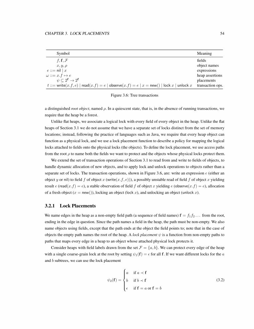
CHAPTER 3. LOCK PLACEMENTS 54
Symbol Meaning
f, f ,F fieldsx, y, ⇢ object names
e ::= nil | x expressions! ::= x.f 7! e heap assertions
✓ 2
f ! 2
f placementst ::= write(x.f, e) | read(x.f) = e | observe(x.f) = e | x = new() | lock x | unlock x transaction ops.
Figure 3.6: Tree transactions
a distinguished root object, named ⇢. In a quiescent state, that is, in the absence of running transactions, werequire that the heap be a forest.
Unlike flat heaps, we associate a logical lock with every field of every object in the heap. Unlike the flatheaps of Section 3.1 we do not assume that we have a separate set of locks distinct from the set of memorylocations; instead, following the practice of languages such as Java, we require that every heap object canfunction as a physical lock, and we use a lock placement function to describe a policy for mapping the logicallocks attached to fields onto the physical locks (the objects). To define the lock placement, we use access pathsfrom the root ⇢ to name both the fields we want to protect and the objects whose physical locks protect them.
We extend the set of transaction operations of Section 3.1 to read from and write to fields of objects, tohandle dynamic allocation of new objects, and to apply lock and unlock operations to objects rather than aseparate set of locks. The transaction operations, shown in Figure 3.6, are: write an expression e (either anobject y or nil) to field f of object x (write(x.f, e))), a possibly unstable read of field f of object x yieldingresult e (read(x.f) = e), a stable observation of field f of object x yielding e (observe(x.f) = e), allocationof a fresh object (x = new()), locking an object (lock x), and unlocking an object (unlock x).
3.2.1 Lock Placements
We name edges in the heap as a non-empty field path (a sequence of field names) f = f
1
f
2
. . . from the root,ending in the edge in question. Since the path names a field in the heap, the path must be non-empty. We alsoname objects using fields, except that the path ends at the object the field points to; note that in the case ofobjects the empty path names the root of the heap. A lock placement is a function from non-empty paths topaths that maps every edge in a heap to an object whose attached physical lock protects it.
Consider heaps with field labels drawn from the set F = {a, b}. We can protect every edge of the heapwith a single coarse-grain lock at the root by setting
1
(f) = ✏ for all f . If we want different locks for the a
and b subtrees, we can use the lock placement
2
(f) =
8>>><
>>>:
a if a � f
b if b � f
✏ if f = a or f = b
(3.2)

CHAPTER 3. LOCK PLACEMENTS 55
(a)⇢
x
y
nil
vz u
a
b
a
b
a
b
(b)⇢
nil
y
nil
v
a
b
a
b
Figure 3.7: Two examples of tree-structured heaps. Nodes (e.g., x, y) represent objects, whereas edges (labeleda, b) represent fields. Node ⇢ is the root object of the heap.
where g � f denotes that g is a strict prefix of f . For example, in Figure 3.7(a), under placement 2
the lockat ⇢ protects the edges from ⇢ to x and from ⇢ to y, the lock at x protects the edges from x to z and from x tou, and the lock at y protects the edge from y to v.
If for a path f the placement path (f) leads to nil in the heap, we use the lock given by the longest non-nilprefix of the path (f); that is, we use the lock on the object immediately preceding the edge to nil in theplacement path. For example, consider the heap of Figure 3.7(b) under the placement
2
. The lock that protectsthe edge named by the path ab according to the placement is
2
(ab) = a, however the edge a from the rootnode ⇢ points to nil. In this case, we use the lock on the longest non-nil prefix of
2
(ab) to protect the edge ab,namely ⇢ itself. In this chapter we only consider the convention of placing locks on the longest non-nil prefix,however other conventions are possible, for example, always placing such locks at the root.
Modifications to the heap may implicitly alter the mapping from logical locks to physical locks. If atransaction updates an edge, then the transaction must hold both before and after the update all logical lockswhose mapping to physical locks may change. For example consider again the lock placement
2
in the contextof the tree heap shown in Figure 3.7(b). According to the placement the lock on ⇢ protects the edge a from theroot; however since edge a points to nil, edges on any path that begins with a are also protected by the lock ata. If a transaction were to set ⇢.a to point to a node w, the lock at w would now protect the edges on paths thatbegin with a; the transaction has split the logical roles of the lock at ⇢ before the write between the lock at⇢ and the lock on node w. Whenever a transaction splits or merges locks (e.g., by setting the field ⇢.a to nil
again), it must hold every lock involved.Figure 3.8(a) shows a trace of a transaction that adds a new edge labeled a from object y to a fresh object
w to the heap of Figure 3.7(b) under placement 2
. The transaction acquires two locks, namely the lock at ⇢that protects the edge from ⇢ to y, and the lock at y that protects the entire subtree rooted at y. We need nothold a lock on w when adding w into the tree; linking w into the heap does not change the association betweenlogical and physical locks, and hence we do not need to hold the lock on w either before or after adding it tothe heap.
If we desire a finer-grain locking, we can use a lock attached to every object to protect the fields of thatobject by using the placement function
3
(gf) = g for any g, f. (3.3)

CHAPTER 3. LOCK PLACEMENTS 56
(a) (b) (c)lock ⇢ lock ⇢ read(⇢.b) = y
read(⇢.b) = y read(⇢.b) = y lock y
observe(⇢.b) = y observe(⇢.b) = y read(⇢.b) = y
lock y lock y observe(⇢.b) = y
w = new () read(y.a) = nil read(y.a) = nil
write(y.a, w) w = new () w = new ()
unlock y lock w lock w
unlock ⇢ write(y.a, w) write(y.a, w)
unlock w unlock w
unlock y unlock y
unlock ⇢
Figure 3.8: Three transaction traces that add a new outgoing edge labelled a from node y to the tree ofFigure 3.7(b) under: (a) the lock placement
2
defined in Equation (3.2), (b) the lock placement 3
defined inEquation (3.3), and (c) the lock placement
4
defined in Equation (3.4).
The lock placement 3
places the lock that protects each edge f on the object at the head of the edge.Figure 3.8(b) shows a trace of a transaction that again adds the edge labeled a from node y to a fresh node w tothe heap of Figure 3.7(b), this time under lock placement
3
. Unlike the transaction of Figure 3.8(a), we needto ensure that by adding the new edge the write does not implicitly change the mapping from edges to locks.The well-lockedness conditions, which we introduce shortly, require that a transaction hold all physical lockswhich may map to different logical locks before and after a write. The operation read(y.a) = nil verifies thatthere is no existing subtree of y reachable via edge a. Before the update the lock at y protects every possibleedge reachable from y.a, however after the write the lock y only protects the edge y.a itself, whereas the lockat w protects everything reachable from node w. Hence we must hold lock w when performing the write, sinceadding the edge splits the lock at y. (In general one must hold locks when connecting objects into the heap;however in this specific case, since the write which links w to the heap is the last write in the transaction itwould be possible to optimize away the lock and unlock.)
Finally, we can use a speculative placement, as in the last section. If we set
4
(f) = f (3.4)
the lock that protects each edge is located at the target of the edge. Figure 3.8(c) once again shows a transactionthat adds a fresh edge labeled a to node w, this time using lock placement
4
. The transaction begins byperforming a speculative read to guess that the identity of the object whose lock protects ⇢.b is y; the transactionthen acquires the lock on y. It is possible that a concurrent write to ⇢.b means that the lock on y no longerprotects ⇢.b, so the transaction must perform the read again. The second read also returns y, and hence weknow that the second read is stable since the transaction already holds lock y. The transaction then performs aread of y.a which returns nil. The value of the placement function for edge y.a is (ba) = ba, however sinceedge ba points to nil, the lock on the longest non-nil prefix of ba protects ba, in this case path b (node y). Since

CHAPTER 3. LOCK PLACEMENTS 57
we hold the lock on y already, we know that the read of y.a is also stable. Finally, the transaction must holdthe lock on w when adding it to the heap to maintain the invariant that a transaction must hold all physicallocks whose logical/physical mapping changes as a consequence of a write.
3.2.2 Well-Locked Transactions
We represent a transaction’s state by three sets L, ⌦, and �. As before, L is the set of locks that transactionholds, and ⌦ is an observation set consisting of stable heap observations of the form x.f 7! e; equivalently,we can think of ⌦ as a transaction’s local part of the heap. We do not require ⌦ be a forest; a transaction maycreate any heap shapes it desires within its local heap, allowing the common idiom of temporarily violatinginvariants and later restoring them during the course of a transaction. However, the forest invariant mustbe restored when the transaction releases objects in its local heap back into the global heap. Enforcing thiscondition is the purpose of the global non-alias set �. An object x is a member of � if the transaction hasshown that there is no globally visible path from the root to x (i.e., the transaction has locked the edge to x).The well-lockedness rules for tree heaps ensure that there is at most one globally-visible edge to any nodeand hence the globally-visible part of the heap is a forest. At the start of every transaction � is the empty set.Transactions add entries to � by discovering global edges to nodes and transferring them into their local heap⌦; entries are removed from � when pointers to objects are released from the stable heap ⌦ back into theglobal heap.
The path alias judgement ⌦ ` f ⇠ x holds if f is a path in ⌦ from the root to location x; that is, if |f | = k,then there is a sequence of nodes v = v
0
v
1
· · · such that (⇢.f0
7! v
0
) 2 ⌦, (vi�1
.f
i�1
7! v
i
) 2 ⌦ for all1 < i < k � 1, and v
k�1
.f
k�1
7! x. We write f 2 ⌦ if the path f from the root vertex exists in ⌦, that is,⌦ ` f ⇠ x holds for some object x.
The restriction of a path f to a local heap ⌦, written f |⌦
is defined as:
f |⌦
=
8>>><
>>>:
f if f 2 ⌦
g where 9g, h. gh � f ^ ⌦ ` gh ⇠ nil
undefined otherwise
The restriction of path f is either f itself if present in ⌦, or a prefix of f leading to nil in ⌦. The restriction of apath is undefined if the path f leaves the local heap ⌦.
We hold the lock on an edge reached via a path if we hold the lock on the node given by correspondinglock placement, restricted to the local heap:
pathlocked
(f ,⌦, L) ::= 9x 2 L. ⌦ ` (f)|⌦
⇠ x
We hold the lock on a field f of an object x under local heap ⌦, global non-alias set � and locks L, writtenlocked
(x.f,⌦,�, L), if we hold the lock protecting field f on every path to field f in the local heap ⌦, and

CHAPTER 3. LOCK PLACEMENTS 58
(TNEW)⌦
0= ⌦ [ {x.f 7! nil | f 2 F} x /2 dom⌦ x /2 � �
0= � [ {x}
⌦,�, L
x = new();⌦
0,�
0, L
(TLOCK)x /2 L
⌦,�, L
lock x;⌦,�, L [ {x}
(TUNLOCK)x 2 L L
0= L \ {x} (⌦
0,�
0) = d⌦;� | L0
; e forest(⌦,⌦
0,�,�
0)
⌦,�, L
unlock x;⌦
0,�
0, L
0
(TOBSERVE)(x.f 7! e) 2 ⌦
⌦,�, L
observe(x.f) = e;⌦,�, L
(TREADUNSTABLE)x.f /2 dom⌦ ⌦
0= ⌦ [ {x.f 7! e} ¬locked
(x.f,⌦
0,�, L)
⌦,�, L
read(x.f) = e;⌦,�, L
(TREADSTABLE)
x.f /2 dom⌦ ⌦
0= ⌦ [ {x.f 7! e}
locked
(x.f,⌦
0,�, L) �
0=
(� if e = nil
� [ {y} if e = y
⌦,�, L
read(x.f) = y;⌦
0,�
0, L
(TWRITE)
x.f 2 dom⌦ ⌦
0= ⌦[x.f 7! y]⇣
8g,h. (⌦ ` g ⇠ x) ^ gf � (h) =) pathlocked
(h,⌦, L) ^ pathlocked
(h,⌦0, L)
⌘
⌦,�, L
write(x.f, y);⌦
0,�, L
Figure 3.9: Well-locked tree heap operations: ⌦,�, L
t;⌦
0,�
0, L
0
furthermore � implies there are no paths to x outside the local heap. Formally,
locked
(x.f,⌦,�, L) ::= x 2 � ^ 8g.�⌦ ` g ⇠ x =) pathlocked
(gf,⌦, L)�
If the local heap ⌦ contains cycles, observe that there may be infinitely many paths g and the locked
predicate is well-defined in this case.The definition of the locked predicate implies the objects that cannot be reached by other transactions are
considered locked. In particular if there is no path from the root to a node x in the local heap ⌦, and we havex 2 �, implying that there is no path to x in the global heap either, then definition of the locked predicateimplies that the fields of x are locked. The well-lockedness rules add freshly allocated objects to � sincethey are created disconnected from the global heap, and updates to such nodes are considered correct by thedefinition of locked, even in the absence of any explicit lock acquisitions.
The judgement ⌦,�, L
t;⌦
0,�
0, L
0 defined in Figure 3.9 captures the class of well-locked tree oper-ations. If the judgement holds, then a transaction that executes operation t under stable observation set ⌦,objects �, and lock set L yields a new stable observation set ⌦0, objects �0 and lock set L0. The (TNEW) rule

CHAPTER 3. LOCK PLACEMENTS 59
states that all of the fields of a newly allocated object x point to nil, and since there can be no path to x in theheap all of x’s fields are stable and x 2 �. As before, the (TLOCK) rule allows a transaction to acquire a lockit does not yet hold and has no affect on either ⌦ or �.
In the (TUNLOCK) rule, the stabilization operator is more involved than in the case of flat heaps, becausewe must compute not just the stable set of heap facts, but also the set of objects for which the transaction haslocked the incoming path: if an edge x.f 7! y drops out of the stable observation set because a lock is released,the transaction can no longer assume it holds locks on all of the paths to object y. The stabilization (⌦
0,�
0) of
a local heap ⌦
0
and global heap �
0
under locks L and placement , written (⌦
0,�
0) = d⌦
0
;�
0
| L; e, is thelimit of the monotonically decreasing sequence:
⌦
i+1
= {x.f 7! e 2 ⌦
i
| locked
(x.f,⌦
i
,�
i
, L)} �
i+1
= �
i
\ {y | x.f 7! y 2 ⌦
i
\ ⌦i+1
}
In addition, rule (TUNLOCK) requires that transactions maintain the forest condition
forest(⌦,⌦
0,�,�
0) ::= 8y.
0
@|{(x.f 7! y) 2 ⌦ \ ⌦0}| =
8<
:1 if y 2 � \ �0
0 otherwise.
1
A
The forest condition ensures that a transaction may only release a pointer to a node y into the global heap ifthere are no other references to y in the global heap (y 2 � \ �0). Furthermore, the condition also ensures thata transaction cannot release two or more pointers to the same location y into the global heap.
The rules (TOBSERVE), (TREADUNSTABLE), and (TREADSTABLE) are similar to the rules in Section 3.1,updated to reflect that the heap now involves objects and fields. Note that (TREADSTABLE) adds the objectthat is the target of the read to � in the case that the field is not nil.
The most interesting rule is (TWRITE). Updating a field x.f to point to y not only changes the paths toy, it changes the paths to every object reachable from y. Thus, as a result of a single field update, the lockplacements may change for y and every edge reachable from y. Furthermore, fields no longer reachable fromx.f after the update also may have altered lock placements. For this reason a transaction must hold locks onevery edge reachable from x.f both before and after the update. These conditions are necessary for safety, butneed not be burdensome if the lock placement has a suitable granularity. For example, if the subtrees rooted atx and y are locked by the locks at x and y respectively, the update requires two locks.
A transaction T = t
1
. . . t
k is well-locked if there exists a sequence of lock sets Li, observation sets ⌦i,and object sets �i such that
L
0
= L
k
= ;, ⌦
0
= ;, �
0
= ;, and ⌦
i�1
,�
i�1
, L
i�1
t
i
;⌦
i
,�
i
, L
i for 1 i k.
A well-locked transaction must begin with all three sets ⌦, �, L empty. Furthermore at the end of the transactionthe set of locks L must be empty again, and hence a transaction must release all of its locks. We do not requirethat ⌦ or � be empty at the conclusion of a transaction; however since the transaction may not hold any locks

CHAPTER 3. LOCK PLACEMENTS 60
on termination, any part of the heap that is stable and in ⌦ with an empty lock set cannot be reachable fromthe global and can be garbage-collected.
Lemma 3.3. Let s be a valid schedule of a set of well-locked transactions {T1
, . . . ,Tk
}. Let ⌦j
i
, �j
i
, and L
j
i
be the set of observations, objects, and locks of each transaction after schedule step j. Let hj be the heap afterschedule step j, and suppose h
0 is a forest. Then for all time steps j:
• the lock sets {Lj
i
}ki=1
are disjoint.
• the observation sets {⌦j
i
}ki=1
are stable, have disjoint domains, and heap h
j is an extension of each{⌦j
i
}ki=1
.
• the sets {�j
i
}ki=1
are disjoint, and
• the global heap h
j less edges present in the local heaps {⌦j
i
}ki=1
is a forest. Furthermore if x 2 �
j
i
thenevery pointer to node x in the heap is an element of some local heap ⌦
j
i
0 .
Proof. By induction on the length of the schedule. The result is immediate for a schedule of length 0. Supposethe result is true for any schedule of length n, and consider any schedule of length n + 1. Without lossof generality, assume transaction number 1 performs the additional operation t
n+1. Since transaction 1 iswell-locked, we know ⌦
n
1
,�
n
1
, L
n
1
t;⌦
n+1
1
,�
n+1
1
, L
n+1
1
holds. There are several possible derivations:
• Rule (TNEW): The result about lock sets is immediate. The concrete semantics of the new operatorguarantee that the result x of allocation is fresh, and hence there are no pointers to x in the heap. Itfollows that all of the fields of x are stable and known only to the current transaction. The result aboutthe observation sets then follows from the induction hypothesis. The result about local heaps and globalheaps is a consequence of the freshness of x and the induction hypothesis.
• Rule (TLOCK): Disjointness of lock sets follows from the validity of the schedule. The other results areimmediate from the induction hypothesis.
• Rule (TUNLOCK): Disjointness of lock sets is immediate. Stability of the current transaction holdsby definition, and for other transactions by the induction hypothesis; unlocking a lock cannot affectother transactions. Disjointness and subsetting hold by the induction hypothesis and the definition ofstabilization. The forest condition ensures that a transaction can evict a pointer to a node x from its localheap only if x 2 �, and hence the global forest condition is preserved given the induction hypothesis.
• Rule (TOBSERVE): Immediate.
• Rule (TREADUNSTABLE): Immediate.
• Rule (TREADSTABLE): The lock set result is immediate. Stability of each transaction’s observation setholds since the rule requires that the transaction hold locks that ensure the newly read heap assertionis stable (locked
(x.f,⌦,�, L)) and the induction hypothesis guarantees all other heap assertions are
CHAPTER 3. LOCK PLACEMENTS 61
stable. The lockedness of x.f ensures that the current transaction must hold the lock for x.f on everypath. No other transaction can have x.f as part of its stable observation set because of the disjointnessof observation sets from the induction hypothesis. The result about � and ⌦ follows from the forestcondition on the heap; if we acquired a stable reference to a node y then it must have been the uniquereference in the global heap, and hence no other transaction may have y 2 � by the induction hypothesis.
• Rule (TWRITE): The lock set result is immediate. The newly written memory location must be stablesince the transaction requires that x.f be present in ⌦ and from the condition that ensures the transactionholds any locks reachable from x.f that may change identity; the latter condition also ensures that thewrite cannot affect the stable observation sets of any other transaction. The disjointness and extensionconditions hold by the induction hypothesis. The result about local and global heaps is immediate fromthe induction hypothesis; a transaction may freely update its local heap since the tree-structure conditionneed only be maintained at at unlock time.
Finally, we have a logical serializability lemma analogous to Lemma 3.2:
Lemma 3.4. Any valid schedule of a set of well-locked, logically two-phase tree transactions {T1
, . . . ,Tk
}is conflict-equivalent to a serial logical schedule.
As in the flat-heap case, these results can be extended to shared/exclusive locks using the approach inSection 3.1.5.
3.3 Transactions on Decomposition Heaps
At the core of the locking protocol of Section 3.2 is the invariant that the global heap is a forest. Since lockplacements are defined using access paths, for soundness the locking protocol must verify that a transactionholds the locks that protect an edge on every possible access path. In a forest this requirement is simple, sincethere can be at most one path between nodes.
In this section we show how to relax the forest restriction and apply lock placements to heaps that aredecompositions (Chapter 2), which may contain multiple paths to the same object. The technical machinerydeveloped so far remains almost unchanged, with the exception that the forest condition is replaced by abounded in-degree condition which ensures that all of the paths to a node are known.
To minimize the complexity of our proof system, and to obtain the most general result possible, in thissection we work with heaps that are a relaxation of decompositions; our proof system enforces just enoughstructure to guarantee that heaps have bounded in-degree, which is the analogue of the forest condition for treeheaps. Enforcing all of the structural conditions mandated by a decomposition would unnecessarily complicatethe well-lockedness rules, and is not necessary to address our main interests in this section, which are thesafety conditions forced on lock placements because of the heap structure.

CHAPTER 3. LOCK PLACEMENTS 62
(a) (b)⇢
y
z
w
v
a
pid
ˆ
b
ns
c
ns
ˆ
d
pid
e
cpu
⇢
y
1
y
2
z
1
z
2
w
1
w
2
w
3
v
1
v
2
v
3
a1a2 b1 b2
c1c2 c1 d1 d2
d3
e1 e2 e3
Figure 3.10: (a): A decomposition heap shape, and (b): a decomposition heap that is an instance of decomposi-tion heap shape (a).
A decomposition heap shape ˆ
h is a rooted, connected, directed acyclic graph (
ˆ
V ,
ˆ
E) consisting of a set ofvertices ˆ
V = {u, v, . . . } and a set of edges ˆ
E ✓ ˆ
V ⇥ ˆ
F ⇥ ˆ
V . To simplify the definition of lock placements,we require that each edge of a decomposition be labeled with a unique name drawn from a set ˆ
F .We will use the decomposition of Figure 3.10(a) as a running example, which depicts a decomposition for
the process scheduler example of Chapter 2. Recall in the scheduler example, every process has associatedfields pid (process ID), ns (name space), and the process’ assigned cpu; a pair of a pid and a ns uniquelyidentify a process. To find the cpu of a particular process using the decomposition, we can first look up theprocess id by following edge a
pid
and then the process’ name space by following edge c
ns
, or we can firstlook up the name space by following edge ˆb
ns
and then the process id by following edge ˆ
d
pid
. For a given pairof process ID and name space, the shared node w in the decomposition shape assures us we will get the sameresult regardless of which path we take.
Like a decomposition, a decomposition heap shape is a static description of a class of heaps. Let in(v) bethe set of field names incoming to v in a decomposition shape and let out(v) be the set of outgoing field names.A heap (V,E) is an instance of a decomposition shape ˆ
d if
• every vertex in V is an instance v
i
of some vertex v 2 ˆ
V ,
• every edge (u
i
, f
j
, v
k
) 2 E is an instance of some (u,
ˆ
f, v) 2 ˆ
E, and
• every vertex v
i
has exactly one instance f
i
of every incoming edge ˆ
f 2 in(v).
The last condition provides a bound on the in-degree of a vertex, which is the key to applying path-based lockplacements to decomposition heaps.
The distinction between a decomposition as defined in Chapter 2 and a decomposition heap shape is thatdecomposition heap shape only requires that each node in the heap have at most one instance of each of theedges given by the decomposition, and does not enforce that all such edges exist. Decomposition heap shapesalso do not attempt to describe or reason about the values attached to each edge or require that those edges formpart of a meaningful relation under an abstraction function. Decomposition heap shapes retain just enough ofthe structural invariants of a decomposition to permit reasoning about lock placements.

CHAPTER 3. LOCK PLACEMENTS 63
Symbol Meaning
u, v decomposition verticesu
i
, v
j
,V object namesˆ
f,
ˆf abstract fieldsf
i
, f
j
, f concrete fieldse ::= nil | v
i
expressions! ::= u
i
.f 7! e heap assertions ✓ 2
f ! 2
f placementst ::= write(u
i
.f , e) | read(ui
.f) = e | observe(ui
.f) = e transaction operations| vi
= new v | lock vi
| unlock vi
Figure 3.11: Transactions on decomposition heaps.
Figure 3.10(b) shows an instance of the decomposition in Figure 3.10(a). Every edge ˆ
f from a vertex u toa vertex v of the decomposition has a corresponding set of edges {f
1
, f
2
, · · · } outgoing from any instance u
i
of u in the corresponding decomposition instance.The well-lockedness rules defined below quantify over all paths that are a suffix of a particular path f . To
keep our transaction-language small, we impose an additional requirement that the set of possible instancesf
i
of each abstract edge ˆ
f be drawn from a bounded set; that is i 2 {1, . . . , k} for some k. The boundedset restriction can be lifted by extending the transaction language with an iteration operation that allows atransaction to iterate over all instances of an edge from a vertex; the addition of iteration gives another way forthe rules to conclude a fact holds for all instances of an abstract edge ˆ
f .The transaction operations on decomposition heaps are almost identical to the set of operations on trees
(Section 3.2), differing only in how objects and fields are named. The transaction operations, shown inFigure 3.11, are: write an expression e (either nil or some v
k
to field f
j
of object ui
(write(ui
.f
j
, e))), apossibly unstable read of field f
j
of object ui
yielding result e (read(ui
.f
j
) = e), a stable observation of fieldf
j
of object ui
yielding e (observe(ui
.f
j
) = e), allocation of a fresh object of type v (vi
= new v), locking anobject (lock v
i
), and unlocking an object (unlock vi
).
3.3.1 Lock Placements
Lock placements are defined exactly as in the tree case: is a function from non-empty heap paths to pathsthat maps every edge in a heap to an object whose lock protects it. Because edges may now have multiplepaths that reach them, a transaction must hold locks on all paths to an edge to perform a stable read or to writethe edge.
We now illustrate some of the possibilities for lock placements on decomposition heaps. For our standardfirst example, by setting
1
(f) = ✏ for all f (3.5)
we can use a single lock at the root of the heap to protect every edge in a decomposition instance. Figure 3.12(a)

CHAPTER 3. LOCK PLACEMENTS 64
Line (a) (b)1: lock ⇢ read(⇢.a
2
) = y
2
2: read(⇢.a
2
) = y
2
lock y
2
3: read(⇢.b
2
) = z
2
read(⇢.a
2
) = y
2
4: observe(⇢.a
2
) = y
2
observe(⇢.a
2
) = y
2
5: observe(⇢.b
2
) = z
2
read(⇢.b
2
) = z
2
6: read(y
2
.c
7
) = nil lock z
2
7: read(z
2
.d
5
) = nil read(⇢.b
2
) = z
2
8: w
4
= new w observe(⇢.b
2
) = z
2
9: write(y
2
.c
7
, w
4
) read(y
2
.c
7
) = nil
10: write(z
2
.d
5
, w
4
) read(z
2
.c
5
) = nil
11: unlock ⇢ w
4
= new w
12: write(y
2
.c
7
, w
4
)
13: write(z
2
.d
5
, w
4
)
14: unlock z
2
15: unlock y
2
Figure 3.12: Example transactions that add a new node w4
with access paths a2
c
7
and b2
d
5
to the decompositionheap instance shown in Figure 3.10(b), under (a) lock placements
1
, defined in Equation (3.5), or 2
, definedin Equation (3.6), and (b) lock placement
3
defined in Equation (3.7).
shows a well-locked transaction that adds a fresh instance of w, namely w
4
, to the heap of Figure 3.10(b) underlock placement
1
. Acquiring the lock on ⇢ protects the entire heap graph; the transaction then adds w4
underboth the access path a
2
c
7
and b
2
d
5
.Another possibility is to use the placement
2
(f) =
8>>><
>>>:
✏ if f 2 {ai
, b
i
, a
i
c
j
, b
i
d
j
}
a
i
c
j
if f = a
i
c
j
e
k
b
i
d
j
if f = b
i
d
j
e
k
(3.6)
which uses a lock at the root to protect instances of edges a, ˆb, c, and ˆ
d, and locks at instances of node w toprotect instances of edge e. Instances of edge e can be reached by two different paths, and thus to observe e atransaction must acquire locks on both paths.
Finally, we can use a speculative lock placement. For example, we could protect instances of edges a and ˆ
b
using speculative locks placed at their targets, and use locks at y and z to protect edges c, ˆd, and e, via the lockplacement
3
(f) = a
i
if ai
� f , and b
j
if bj
� f (3.7)
Figure 3.12(b) again shows a transaction that adds a fresh instance w4
of node w, this time under the speculativelock placement
3
.

CHAPTER 3. LOCK PLACEMENTS 65
3.3.2 Well-Locked Transactions
As in the case of tree heaps we represent the state of a transaction using three sets: the local heap ⌦, a set oflocks L, and the global non-alias set �. Sets ⌦ and L are defined as for trees, but we extend the definition of �to DAGs with bounded sharing.
The purpose of � is to track objects for which the transaction holds locks on incoming edges. In particular,if a transaction does not hold locks on some incoming edges to an object o, then there may be a path from theglobal heap to o and the transaction cannot rely on the stability of o’s fields. Thus � is the transaction’s viewof the global heap and what other transactions might be able to do to objects of interest to the transaction. Theglobal non-alias set � is a mapping from each vertex v
i
in the heap to the subset of the incoming edge labelsof the decomposition in(v) known to be absent from the global heap (i.e., either non-existent or locked by thetransaction). We maintain the invariant that in the global heap there is at most one edge to any instance of adecomposition vertex v labeled with an instance of each ˆ
f 2 in(v). If �(vi
) = ;, then v
i
may have an instanceof each incoming edge in in(
ˆ
f) in the global heap. If �(vi
) = { ˆf} then v has no incoming edge in the globalheap labeled with an instance of ˆ
f . If �(v) = in(v) then v has no incoming edges from the global heap.As before, we hold the lock on an edge reached via a path if we hold the path’s corresponding lock
placement, restricted to the heap:
pathlocked
(f ,⌦, L) ::= 9vi
2 L. ⌦ ` g ⇠ v
i
^ (f)|⌦
= g,
where (f)|⌦
is the restriction of path (f) to heap ⌦, defined in Section 3.2.2.The judgement ⌦,� ` exposed(x) holds if there may be a path to vertex x in the heap that does not lie
entirely in the stable observation set ⌦; the judgement is defined by the inference rules:
�(v
k
) 6= in(v)
⌦,� ` exposed(v
k
)
⌦,� ` exposed(u
i
) ^ (u
i
.f
j
7! v
k
) 2 ⌦
⌦,� ` exposed(v
k
)
We hold the lock on a field x.f if we hold a lock on that field on every path in the local heap, and there areno paths to x outside the local heap.
locked
(v
i
.f
j
,⌦,�, L) ::= ¬exposed(vi
) ^ 8g. (⌦ ` g ⇠ v
i
=) pathlocked
(gfj
,⌦, L))
The judgement ⌦,�, L
t;⌦
0,�
0, L
0 defined by the rules in Figure 3.13 describes the class of well-lockeddecomposition operations, analogous to the class of well-locked tree operations of Section 3.2. The judgementholds if a transaction executing operation t under local heap ⌦, global non-alias set �, and locks L yields anupdated local heap ⌦
0, global non-alias set �0, and lock set L0. The (DNEW) rule states that the fields of anewly allocated object v
i
point to nil; furthermore there can be no heap paths to a freshly allocated objectso assertions about the fields of v
i
are stable and �(v
i
) = in(v). The (DLOCK) rule allows a transaction toacquire a lock that it does not hold at any time.

CHAPTER 3. LOCK PLACEMENTS 66
(DNEW)
⌦
0= ⌦ [ {v
i
.f
j
7! nil | ˆ
f 2 out(v)}v
i
/2 dom⌦ �
0= �[v
i
7! in(v)] v
i
/2 dom�
⌦,�, L
v
i
= new v;⌦
0,�
0, L
(DLOCK)v
i
/2 L
⌦,�, L
lock v
i
;⌦,�, L [ {vi
}
(DUNLOCK)v
i
2 L L
0= L \ {v
i
} (⌦
0,�
0) = d⌦;� | L0
; e balias(⌦,⌦
0,�,�
0)
⌦,�, L
unlock v
i
;⌦
0,�
0, L
0
(DOBSERVE)(u
i
.f
j
7! e) 2 ⌦
⌦,�, L
observe(u
i
.f
j
) = e;⌦,�, L
(DREADUNSTABLE)u
i
.f
j
/2 dom⌦ ⌦
0= ⌦ [ {u
i
.f
j
7! e} ¬locked
(u
i
.f
j
,⌦
0,�, L)
⌦,�, L
read(u
i
.f
j
) = e;⌦,�, L
(DREADSTABLE)
u
i
.f
j
/2 dom⌦ ⌦
0= ⌦ [ {u
i
.f
j
7! e}
locked
(u
i
.f
j
,⌦
0,�, L) �
0=
(� if e = nil
�[v
i
7! �(v
i
) [ { ˆf}] if e = v
i
⌦,�, L
read(u
i
.f
j
) = e;⌦
0,�
0, L
(DWRITE)
u
i
.f
j
2 dom⌦ ⌦
0= ⌦[u
i
.f
j
7! e]⇣8g,h. (⌦ ` g ⇠ u
i
) ^ gf � (h) =) pathlocked
(h,⌦, L) ^ pathlocked
(h,⌦0, L)
⌘
⌦,�, L
write(u
i
.f
j
, e);⌦
0,�, L
Figure 3.13: Well-locked decomposition operations: judgement ⌦,�, L
t;⌦
0,�
0, L
0.
The (DUNLOCK) rule allows a transaction to release any lock that it holds; the rule applies the stabilizationoperation to remove any newly unstable facts from ⌦. Similar to the tree case, the stabilization (⌦
0,�
0) of a
local heap ⌦
0
and global heap �
0
under locks L and placement , written (⌦
0,�
0) = d⌦
0
;�
0
| L; e, is thelimit of the monotonically decreasing sequence:
⌦
i+1
= {uj
.f
k
7! e 2 ⌦
i
| locked
(u
j
.f
k
,⌦
i
,�
i
, L)}
�
i+1
= �
i
\ {vk
7! ˆ
f | ui
.f
j
7! v
k
2 ⌦
i
\ ⌦i+1
}
To ensure that there is at most one instance of any edge label ˆ
f 2 in(v) in the global heap, the rule requires thebounded alias condition
balias(⌦,⌦
0,�,�
0) ::= 8v
k
.
0
@|{ui
.f
j
| (ui
.f
j
7! v
k
) 2 ⌦ \ ⌦0}| =
8<
:1 if ˆ
f 2 �(v
k
) \ �0(v
k
)
0 otherwise.
1
A

CHAPTER 3. LOCK PLACEMENTS 67
The bounded alias condition is exactly analogous to the forest condition of Section 3.2.2, and ensures that atransaction may only release an edge with abstract label ˆ
f to a node v
k
into the global heap if there are noother edges to v
k
labeled ˆ
f in the global heap ( ˆf 2 �(v
k
) \ �0(v
k
)). Further the condition forbids releasingtwo pointers with the same label ˆ
f to the same node v
k
into the global heap.Rule (DOBSERVE) states that a transaction may logically observe stable facts about the heap. The
(DREADUNSTABLE) rule allows a transaction to read a value speculatively at any time, however unstablereads do not update ⌦ or �. A transaction may perform a stable read of a pointer if it holds the appropriatelock, transferring the pointer from the global heap into ⌦ and updating � accordingly. Finally, a transactionmay write to a field if it holds the associated lock, and further holds locks on any edges whose logical/physicalmapping may implicitly change as a result of the update.
A transaction T = t
1
. . . t
k is well-locked if there exists a sequence of lock sets Li, observation sets ⌦i,and global non-alias sets �i such that
L
0
= L
k
= ;, ⌦
0
= ;, �
0
= ;, and ⌦
i�1
,�
i�1
, L
i�1
t
i
;⌦
i
,�
i
, L
i for 1 i k.
Lemma 3.5. Let s be a valid schedule of a set of well-locked transactions {T1
, . . . ,Tk
}. Let ⌦j
i
, �j
i
, and L
j
i
be the set of observations, global non-alias sets, and locks of each transaction after schedule step j. Let hj bethe heap after schedule step j, and suppose the part of h0 reachable from the root has a decomposition heapshape. Then for all time steps j:
• the lock sets {Lj
i
}ki=1
are disjoint,
• the observation sets {⌦j
i
}ki=1
are stable, disjoint, and heap h
j is an extension of each {⌦j
i
}ki=1
, and
• the global non-alias sets {�i
}ki=1
are disjoint.
• Let heap h be the heap h
j less edges present in the local heaps {⌦j
i
}ki=1
. Then for every vertex v 2 h
and edge label ˆ
f 2 in(v) either there is exactly one edge labeled with an instance of ˆ
f pointing to v inh, or ˆ
f 2 �
j
i
for some i and there are no edges labeled with an instance of ˆ
f pointing to v in h.
Proof. The structure of the proof (by induction on the length of the schedule) is the similar to the correspondingproofs flat-heaps and trees. The case analysis is also almost the same as for trees; we discuss the two caseswhere there is some variation:
• Rule (DUNLOCK): Disjointness of lock sets is immediate. Stability of the transaction performing theunlock holds by definition, and for other transactions by the induction hypothesis. The disjointnessand extension properties on the local heaps hold by the definition of stabilization and the inductionhypothesis. The side condition on the definition of stabilization ensures that a transaction may onlyrelease a pointer to a vertex v with label f into the heap only if ˆ
f 2 �(v), and hence the condition onedges in the heap holds.
CHAPTER 3. LOCK PLACEMENTS 68
• Rule (DREADSTABLE): The lock set result is immediate. Stability of the observation sets holds by theinduction hypothesis and because the rule requires locked
(u
i
.f
j
,⌦
n+1
1
,�
n+1
1
, L
n+1
1
) as a precondition.The induction hypothesis guarantees that transactions have disjoint observation sets; furthermore thedisjointness of the � sets guarantees that only one transaction can hold the lock on u
i
.f
j
at any time.The result follows from the induction hypothesis and the definition of stabilization.
Finally, we have a logical serializability lemma similar to Lemma 3.2 and Lemma 3.4.
Lemma 3.6. Any valid schedule of a set of well-locked, logically two-phase decomposition transactions{T
1
, . . . ,Tk
} is conflict-equivalent to a serial logical schedule.
And, again, as in the flat heap case, these results can be extended to shared/exclusive locks using theapproach in Section 3.1.5.
3.4 Related Work
Two-phase locking was originally introduced in the context of transactions operating over abstract entities,each with its own associated lock [Eswaran et al., 1976]. The core technical idea of this chapter is that wecan use two-phase locking to show serializability of a wide class of locking strategies by adding a layer ofindirection between logical locks, which are the entities that are the subject of the original two-phase lockingprotocol, and the physical locks that implement them. The original paper on two-phase locking made explicitthe idea of locking not just objects, but program predicates [Eswaran et al., 1976]. Other authors have exploredusing predicate locks; for example, Deshmukh et al. [2010] explored deriving predicate locks from sequentialcorrectness proofs. Logical locks are also examples of predicate locks, which we realize in practice by mappinglogical locks onto physical locks using a lock placement.
Various authors have investigated techniques for inferring locks to implement atomic sections [McCloskeyet al., 2006; Hicks et al., 2006; Emmi et al., 2007; Halpert et al., 2007; Cherem et al., 2008; Cunningham et al.,2008; Zhang et al., 2008]. A related problem is automatically optimizing programs with explicit locking bycombining multiple locks into one [Diniz and Rinard, 1998]. A key part of this class of work is constructing amapping from program objects to the locks that protect them, similar to our lock placement language. Mostexisting work only considers very simple mappings between data and locks; typically data is protected eitherby global locks or by locks on the object which contains the data. The lock placements we propose are muchmore flexible; in particular existing formalisms cannot handle the class of path placements we propose in thischapter, such as speculative locks, or lock placements that vary with heap updates. Our work provides a moregeneral framework for describing the relationship between locks and data, which may be useful to researchersexploring automatic lock inference.
A novel feature of the infrastructure we develop in this chapter is that it allows us to reason about speculativelock placements. Speculative locking is used in highly concurrent libraries and in the context of software

CHAPTER 3. LOCK PLACEMENTS 69
transactional memory [Bronson et al., 2010a; Bronson, 2011; Bronson et al., 2010b]. Although we present ourideas in the context of speculative placements of pessimistic locks, the idea of a lock placement can also beused to reason about the safety and consistency of speculative placements of optimistic STM metadata as usedin practice.
A variety of locking protocols have been proposed in the literature that extend two-phase locking to handledynamically changing heaps and to allow early release. Notable examples include the dynamic tree lockingand dynamic DAG locking protocols [Attiya et al., 2010], and domination locking [Golan-Gueta et al., 2011].Unlike existing protocols which use the lock on each object to protect that object’s fields, our work exploresa more flexible space of mappings between locks and data, where locks and data need not be adjacent. Akey concern of many locking protocols is early release, which allows a transaction to release locks earlierthan would otherwise be permitted by two-phase locking. We do not consider early release in our work;however early release is orthogonal to lock placement, and lock placements could be profitably combined withtechniques for early release.
The concept of a stable set and stabilization is related to rely-guarantee logic [Jones, 1981] and its subse-quent developments [Wickerson et al., 2010]. Concurrent extensions of separation logic, such as ConcurrentSeparation Logic [O’Hearn, 2007], RGSep [Vafeiadis and Parkinson, 2007] and work on storable locks [Gots-man et al., 2007] allow local reasoning about programs with shared mutable state that is accessed concurrently.Our work complements work on direct reasoning about concurrent code; we propose a locking protocol, pa-rameterized by a declarative lock placement, by which we can show conflict-serializability, thereby removingthe need for direct concurrent reasoning for programs that obey the locking protocol.

Chapter 4
Concurrent Data RepresentationSynthesis
In this chapter, we extend the data representation synthesis approach of Chapter 2 to support concurrency,leveraging using lock placements of Chapter 3 to describe the space of possible locking strategies.
Consider the problem of implementing concurrent operations on a directed graph. We must decide howto represent the graph as a collection of data structures, perhaps using a lookup table mapping each node tothe set of its adjacent nodes. We will need to pick concrete representations for both the lookup table (e.g., aconcurrent hashmap) and the adjacency sets (e.g., linked lists). We must also decide how concurrency will berealized. We could add our own synchronization using locks and/or we could use a concurrent container datastructure to implement the lookup table, the sets of adjacent nodes, or both.
Assume for the moment that we decide both containers will be concurrent. We must of course ensurethere is enough synchronization to avoid harmful races, but not so much that we either limit scalability orintroduce deadlocks. Using off-the-shelf concurrent containers can simplify this task, but even using concurrentcontainers for both data structures does not automatically imply that high-level graph operations that touchboth structures (such as inserting or removing an edge from the graph) are correct. In fact, recent work inbug detection for concurrent programs has shown that programmers fail to use standard concurrent containerscorrectly as often as 44% of the time, especially when they must compose multiple concurrent operations[Shacham et al., 2011].
On the other hand, it may be more efficient to have only the top-level lookup table be concurrent and usenon-concurrent data structures for the sets of adjacent nodes—if it is very infrequent that threads try to accessthe same node simultaneously the extra overhead of a concurrent data structure for the adjacency sets won’t beworthwhile. This design has different correctness requirements and would likely result in a different choiceof where to place any needed synchronization to guarantee correctness. The right answer to the decision ofwhether to use a concurrent or non-concurrent data structure for the adjacency sets likely depends on the
70

CHAPTER 4. CONCURRENT DATA REPRESENTATION SYNTHESIS 71
typical workload and it will be difficult to modify the interlinked synchronization and data structures if wedecide later that the graph should be implemented differently.
In this chapter we present an approach to synthesizing concurrent data representations, meaning thatfrom a high-level specification of data we produce both the concrete data structures and the correspondingsynchronization to implement the specification. In our approach, programs are written using concurrentrelations (Section 4.1), a generalization of standard concurrent collections to relations with a concurrentinterface to perform insertions, deletions, and lookups of tuples. Our compiler automatically synthesizes allaspects of the data representation, including the choice of data structures and how they interact, the number andplacement of locks to guard access to those data structures (including, for example, whether locking should befine-grain or coarse-grain), an order in which locks can be acquired to guarantee deadlock freedom, and all ofthe code to correctly manage the interplay of the data structures and synchronization.
Our method builds on the results presented in the two previous chapters (Section 4.3): we use the decom-positions of Chapter 2 to describe how relations can be decomposed into a set of cooperating data structures,and we use the theory of lock placements of Chapter 3 to describe the space of possible locking strategies. Thespecific contributions of this chapter are:
• We introduce concurrent relations, a generalization of standard concurrent container data structures tocontainers of tuples, with concurrent operations to insert, remove, and query relations (Section 4.1).
• The selection of data structures is subtler than in the non-concurrent case, because there is the addeddimension of using concurrent container structures, which may or may not require additional synchro-nization depending on the relational specification, and, in addition, different concurrent containersprovide varying guarantees about the safety of concurrent access. We give a taxonomy of containers andtheir properties relevant to concurrent data representation synthesis (Section 4.2).
• We extend the relational decomposition language of Chapter 2 to support concurrent relations. Just asthe original decomposition language describes how to assemble a representation of a relation from alibrary of container data structures, concurrent decompositions describe how to compose concurrentand non-concurrent data structures together with locks to implement a concurrent relation primitive(Section 4.3).
• We show how to integrate the lock placements of Chapter 3, which describe a space of possible lockingstrategies on data structures, with the problem of selecting the data structures themselves. The choice ofdata structures and lock placements is done in such a way that the resulting code is guaranteed to ensurethe serializability of relational operations (Section 4.3.1).
• We adapt and generalize the problem of selecting a good implementation of the relational primitives,called query planning, to concurrent relations (Section 4.4). One of the major issues is ensuring deadlockfreedom, which we accomplish by selecting a global lock ordering that all relational operations obey byconstruction. We did not previously address deadlock in Chapter 3.

CHAPTER 4. CONCURRENT DATA REPRESENTATION SYNTHESIS 72
• The optimal decomposition depends on the usage patterns of the data structure and the target machine.We present results from a full implementation, which includes an autotuner that allows us to discover agood combination of both locks and container data structures automatically for a training workload. Weperform an evaluation of a concurrent graph benchmark, showing that the best data representation varieswith the workload, and thus it is important to have the flexibility to easily alter the representation ofconcurrent data (Section 4.5).
4.1 Concurrent Relations
We provide five operations for creating and manipulating concurrent relations: empty, remove, update, query,and insert. The relational compiler ensures that the implementations of all relational operations are linearizable[Herlihy and Wing, 1990] (equivalently serializable, since the relational operations are single operationtransactions on a single object). Operations on an object are linearizable if every operation appears to takeplace atomically at a single point in time in between its invocation and response.
The first four operations have the same mathematical specification as their non-concurrent counterpartsdefined in Section 2.1. Recall that empty () creates a new empty relation. Operation remove r s removes tuplesmatching s; in the concurrent case our implementation requires that s be a key for the relation. Operationupdate r s u applies the updates in tuple u to the tuple matching s in relation r, if any; s must be a key for therelation. Finally, operation query r s C returns columns C of all tuples in r matching tuple s.
The only operation with a different specification from its non-concurrent counterpart is the insertionoperation,
insert r s t = if @u. u 2 !r ^ s ✓ u then r !r [ {s [ t},
which inserts a new tuple x, where x is the union of the columns of tuples s and t, into a relation r, providedthere is no existing tuple in r matching s. We require that s and t have disjoint domains.
Insert generalizes the put-if-absent operation provided by standard concurrent key-value maps: put-if-absent(k,v) inserts value v into the map if no other value is already associated with key k, and would bewritten
insert r hkey : ki hvalue: vi
As in the non-concurrent case insert operations may violate functional dependencies, and it is the client’sobligation to ensure functional dependencies are observed. In the non-concurrent case, a client could performa query to check whether a functional dependency would be violated by a subsequent insertion; this approachis not possible in a concurrent setting since a concurrent thread could change the relation between the queryand the subsequent insert. The revised form of the insert operation allows clients to atomically test whetherfunctional dependencies will be satisfied by a new tuple even in the presence of concurrent updates.
For example, consider a relation representing the edges of a directed graph, with columns {src, dst ,weight}

CHAPTER 4. CONCURRENT DATA REPRESENTATION SYNTHESIS 73
satisfying the functional dependency src, dst ! weight . We can create a new, empty graph relation r
0
usingthe empty () operation. Inserting an edge
insert r
0
hsrc: 1, dst : 2i hweight : 42i
results in a new relation r
1
= {hsrc: 1, dst : 2, weight : 42i}. A subsequent insertion
insert r
1
hsrc: 1, dst : 2i hweight : 101i
leaves the relation unchanged, because relation r
1
already contains an edge with the same src and dst fields.
4.2 A Taxonomy of Concurrent Containers
Concurrent decompositions are an extension of the non-concurrent decompositions of Chapter 2, and describehow to implement concurrent relations as a combination of both concurrent and non-concurrent data structures.Before diving into the details of the concurrent decomposition language (Section 4.3), we first describe theconcurrency properties of the container data structures found in the wild, which form the building blocks ofconcurrent decompositions.
Container Interface A container is a data structure that implements an associative key-value map interfaceconsisting of read operations lookup(k) and scan(f), and a write operation write(k, v).
• The lookup operation lookup(k) returns the value associated with a key k, if any.
• The scan operation scan(f) iterates over the map, and invokes the function f(k, v) once for each key k
and its associated value v in the map. A scan may or may not return the entries of the map in sortedorder.
• The write operation write(k, v) sets the value associated with a key k to v. Here v is an optional value,in the style of ML. If v is Some w, then the operation updates the value associated with key k to w,whereas if v is None, representing the absence of a value, then any existing value associated with k isremoved. The write operation subsumes operations to insert, update, and remove entries from a map.
4.2.1 Concurrency Safety and Consistency
We next discuss two related properties of containers, concurrency safety, which describes whether it is safe fortwo operations to occur in parallel, and consistency, which characterizes what a container guarantees aboutthe possible orders of events in a concurrent execution. Table 4.1 lists the concurrency safety and consistencyproperties of a selection of Java containers from the JDK; as we show, containers differ greatly in their supportfor concurrency.

CHAPTER 4. CONCURRENT DATA REPRESENTATION SYNTHESIS 74
Data Structure Concurrency-safetylookup/lookup lookup/write scan/write write/writelookup/scanscan/scan
HashMap yes no no noTreeMap yes no no noConcurrentHashMap yes yes weak yesConcurrentSkipListMap yes yes weak yesCopyOnWriteArrayList yes yes yes yes
Table 4.1: Concurrency safety properties of selected containers from the JDK. Possible operations are lookup,scan, or write. For an operation pair ↵/�, concurrently executing operations ↵ and � on a container is eitherunsafe (“no”), safe but only weakly consistent (“weak”), or both safe and linearizable (“yes”).
Concurrency Safety For a given data structure, we say a pair of operations ↵/� is concurrency-safe if twothreads may safely execute operations ↵ and � in parallel with no external synchronization. A container isconcurrency-safe if all pairs of operations are concurrency-safe. Concurrency safety is strictly a statementabout the correct usage of the interface of a data structure; it is irrelevant how the data structure guaranteessafety internally, whether by locks, atomic instructions, or by some other means.
Consider the data structures described in Table 4.1. Almost all data structures support parallel readoperations; for example concurrent threads may safely read or iterate over a Java HashMap in parallel withoutsynchronization. Exceptions exist; for example, it would not be safe for threads to perform concurrent reads ofa splay tree because splay tree read operations rebalance the tree.
Only a few containers permit write operations in parallel with other operations. For example, it is unsafe toread from or write to a HashMap object while another thread is writing to the same HashMap. By contrast aConcurrentHashMap or a CopyOnWriteArrayList allow concurrent lookup and write operations, or pairsof concurrent write operations. On a concurrency-safe container, such as a ConcurrentHashMap, the lookup
and write operations are linearizable even in the absence of any external concurrency control. For concurrency-unsafe operations, such as reading a splay tree, linearizability is the responsibility of an external concurrencycontrol primitive, such as a lock.
The scan operation, however, behaves differently. Even many containers that allow iteration in parallel withmutation do not guarantee that iteration is linearizable. We identify two different possibilities. Some containers,such as ConcurrentHashMap provide weakly consistent concurrent iteration; that is, concurrent iteration issafe, but may or may not reflect inserts and removals that occur in parallel with the iteration. Iteration over aweakly-consistent container may not be linearizable, that is, the result of the iteration may not correspond tothe set of entries present in the container at any instant in time. Conversely for containers that provide snapshotiteration, such as a CopyOnWriteArrayList, iteration behaves as if it operated over a linearizable snapshotof the container.

CHAPTER 4. CONCURRENT DATA REPRESENTATION SYNTHESIS 75
4.3 Concurrent Decompositions
The concurrent decomposition language describes how to assemble container data structures into represen-tations of relations that support concurrent serializable transactions that implement the various relationaloperations. By combining concurrent and non-concurrent data structures with locks we can build a representa-tion of a relation with strong concurrency guarantees, even if the constituent data structures themselves havelimited support for concurrency.
We extend the relational decomposition language of Chapter 2 to support concurrent operations frommultiple threads. Two key ideas underlie safe and scalable concurrent decompositions: leveraging existingconcurrent containers to the full extent possible, and supplementing containers with locks as necessary toensure the safety and serializability of concurrent transactions over the complete decomposition. Formally, aconcurrent decomposition is a decomposition extended with a lock placement that describes the number andplacement of locks, and the association between locks and data (Section 4.3.1).
We use Figure 4.1(a) as a running example, which shows a decomposition for a filesystem directory treerelation, based on the directory entry cache in the Linux kernel. The relation has three columns parent , name ,and child and obeys a functional dependency parent ,name ! child . Each ‘parent’ directory entry has zeroor more ‘child’ directory entries, each with a distinct file ‘name’.
In Figure 4.1(a), the edge ⇢x from the root indicates that the relation is implemented by a TreeMap
from each parent value to the residual relation of all (name, child) pairs for that parent. Recursively, thissubrelation is implemented by another TreeMap from name to the child directory (edge xy). Finally, thefunctional dependency guarantees that the child directory is a singleton tuple and is implemented by its singlevalue (edge yy). This structure (a map from parents to the set of child directory names) enables efficientiteration over the children of a directory, which is useful when, for example, unmounting a filesystem. Toenable efficient directory lookup the decomposition also includes a global hashtable mapping (parent ,name)
pairs to child objects (edge ⇢y).Figure 4.1(b) depicts an instance of the decomposition of Figure 4.1(a) representing the relation containing
three directory entries:
{ hparent : 1, name: ‘a’, child : 2i ,hparent : 2, name: ‘b’, child : 3i ,hparent : 2, name: ‘c’, child : 4i}.
4.3.1 Logical Locks, Transactions, and Serializability
Locks Given a decomposition d, we compile each relational operation into a transaction tailored to d. Forsafety and consistency transactions must acquire locks that protect the invariants upon which a transactionrelies. By “lock” here we mean a class of pessimistic synchronization primitives that may be held by atransaction in either of two different modes, namely shared or exclusive.

CHAPTER 4. CONCURRENT DATA REPRESENTATION SYNTHESIS 76
(a) (b)⇢
x
y
{parent}⇢
{parent,name}
⇢
{name} x
{child} y
⇢
0
x
1
x
2
y
1
y
2
y
3
2
1
‘c’ ‘b’‘a’
2,‘c’1,‘a’
2, ‘b’
4 3 2
Key: = TreeMap = ConcurrentHashMap = singleton
Figure 4.1: (a): A decomposition representing a directory tree relation with three columns: parent , name,and child ; and (b): an instance of decomposition (a). Each edge of the decomposition is labeled with a set ofcolumns {· · · }, together with the label of the node whose lock protects instances of that edge (Section 4.3.2).Each edge of the instance is labeled with a valuation for the corresponding decomposition edge’s columns.Solid edges indicate a TreeMap, dashed edges represent a ConcurrentHashMap, and self-loops representsingleton tuples.
Logical Locks To ensure that transactions are serializable, the data in decomposition instances are protectedby logical locks. We associate a distinct logical lock with every edge uv
t
of a decomposition instance. Logicallocks protect the state, either presence or absence, of an edge instance. If a transaction observes the presenceor absence of an edge it must hold shared access to the corresponding logical lock, and if a transaction adds orremoves an edge it must hold exclusive access to the corresponding logical lock. Logical locks are defined forevery possible edge instance, irrespective of whether the edge is actually present in a particular decompositioninstance or not.
For now, we leave the implementation of each logical lock uv
t
abstract. In Section 4.3.2, we implementlogical locks using a smaller set of physical locks attached to the nodes of a decomposition instance. Byplacing restrictions on the possible mappings from logical locks to physical locks we can ensure that containers(concurrent or not) and compositions of containers are used safely.
4.3.2 Physical Locks and Lock Placements
By associating a unique logical lock with every edge instance we can use two-phase locking to ensure thattransactions are serializable. Such an approach would be impractical to implement directly, however. Eachedge instance corresponds to a entry in a container in the heap, and it would often be too slow to actually uselocks at such a fine granularity, not to mention the practical problem that there are infinitely many logical locksdefined for container entries that are absent. Further, as shown in Table 4.1, in practice different containers havedifferent levels of support for safe concurrency, and so while we must use locks to protect some containersfrom all concurrent accesses, in other cases we can rely on the container to mediate concurrent access. Finally,since we treat container implementations as black boxes, we have no way to attach locks to the edge instancesdirectly.

CHAPTER 4. CONCURRENT DATA REPRESENTATION SYNTHESIS 77
(a)⇢
u
v
⇢src
⇢dst
⇢weight
(b)⇢
u v
w
y
⇢src ⇢dst
udst vsrc
wweight yweight
(c)⇢
x
y
z
xsrc ydst
xdst ysrc
zweight
Key: = TreeMap = ConcurrentHashMap = singleton
Figure 4.2: Three concurrent decompositions for a directed graph relation: (a) a “stick”, with a single coarselock around non-concurrent data structures, (b) a “split” decomposition, with locks at different granularities,and (c) a “diamond”, with a mixture of speculatively-locked concurrent data structures and non-concurrent datastructures. Solid edges indicate TreeMap containers, dashed edges represent ConcurrentHashMap containers,and self-loops represent singleton tuples. Each edge is labeled with a set of columns on the left and theassociated lock placement on the right.
Instead of literally maintaining one lock for every possible edge instance, we implement logical locksusing a smaller set of physical locks attached to instances of nodes in a decomposition. We describe thecorrespondence between logical and physical locks using a lock placement, introduced in Chapter 3, which is amapping from the set of logical locks onto the set of physical locks. Many logical locks may map onto thesame physical lock, and acquiring a physical lock corresponds to taking all of the corresponding logical locks.By choosing different lock placements we can describe different granularities of locking. Since physical locksare attached to node instances, in general there may be an unbounded number of physical locks.
Physical Locks To each node v in a decomposition we attach a set of physical locks {v0, v1, . . . }. If thereis only a single physical lock attached to a node we simply write v for both the node and its unique physicallock. Having multiple physical locks per node allows us to protect different outgoing edges from a node withdifferent locks, reducing contention.
Lock Placements A lock placement is a function mapping the logical lock associated with each edge ontoa physical lock on a node that implements it. We define lock placements on the (static) decomposition whichwe extend to (dynamic) decomposition instances in the obvious way; if a lock placement maps the logicallock on edge e to a physical lock on node v at compile time, then at runtime the compiler maps the logicallock on edge instance e
t
onto the physical lock on the corresponding node instance v
t
.Recall the directed graph example from Section 4.1. The relation in question has three columns: src,
dst , and weight , related via the functional dependency src, dst ! weight . Figure 4.2 shows three possibledecompositions, each with a different choice of data structures and lock placements.
Figure 4.2(a) uses a coarse-grain lock placement
1
(e) = ⇢ for all edges e,
CHAPTER 4. CONCURRENT DATA REPRESENTATION SYNTHESIS 78
which protects all edges of the decomposition using a single lock at the root ⇢. Since there is only one instanceof the root node ⇢ in any decomposition instance, the same lock is used to protect everything. Further, sincethe logical locks of all edge instances are mapped to the same physical lock ⇢, the lock serializes access to theentire decomposition data structure, ensuring that each (non-concurrent) TreeMap is only accessed by onetransaction at a time.
Figure 4.2(b) depicts a fine-grain locking strategy decomposition in which each edge is protected by a lockat its head (i.e., objects in a container are protected by a single lock on the container itself), using the lockplacement
2
(↵�) = ↵ for all edges ↵�.
Edges ⇢u and ⇢v are protected by a lock at ⇢, whereas edges uw, vy, wx and yz are protected by locks at u, v,w and y, respectively.
Both of the example lock placements described so far use a single lock to protect all the entries in eachcontainer. Figure 4.2(c) makes use of speculative locking (Section 4.3.4), one of two extensions which allowdifferent dynamic instances of an edge in the same container to be protected by different locks. We deferfurther discussion of this example to Section 4.3.4.
Well-Formed Lock Placements We require that all lock placements satisfy the following conditions:
• The lock placement (uv) of each edge uv either must dominate the edge’s source vertex u or beequal to v. (The latter case occurs in the speculatively-placed locks of Section 4.3.4.) By definitionthis condition ensures that the lock placement for an edge lies on every path from the root of thedecomposition including that edge. This condition ensures the instance of the node (uv) named by thelock placement is unique for each edge instance uv
t
. The domination requirement also simplifies queryplanning (Section 4.4), since it ensures that a query plan will always encounter the necessary locks foreach edge no matter how the edge is reached.
• All edges between an edge and its lock placement share the same placement. That is, fix any edge uv
and take any edge xy in a path in the decomposition from (uv) to u. Then we have (xy) = (uv).This requirement ensures that if a lock protects an edge, then the lock also protects the path from thelock to that edge, thereby ensuring that if we hold a lock then the set of edges protected by that lockcannot change.
Logical Lock Implication Since we implement logical locks by mapping them onto a smaller set of physicallocks, a transaction cannot acquire logical locks directly. Instead, a transaction must acquire physical locksthat imply access to the logical locks that the transaction requires.
We say that a set of physical locks P held by a transaction imply exclusive or shared access, respectively,to the logical lock of edge instance uv
t
under lock placement if:

CHAPTER 4. CONCURRENT DATA REPRESENTATION SYNTHESIS 79
• the transaction holds exclusive or shared access, respectively, to the corresponding physical lock, that is,if (uv) = x then x
t
2 P , and
• the mapping between the logical lock to the corresponding physical lock is stable, that is, there exists apath w
t
from the root of the decomposition instance to v
t
such that the transaction holds shared accessto every edge in w
t
.
The stability criterion means that a physical lock only covers a logical lock if the transaction also holds locksthat guarantee that the logical lock does in fact correspond to that physical lock; if not, a concurrent transactionmight alter the heap and change the association between logical and physical locks. For example, consider aconcurrent hashtable where the elements of each hash bucket are guarded by a lock. If a transaction movesan element v from bucket b
1
to bucket b2
the lock guarding access to v changes, and any transaction thatwas concurrently accessing v by acquiring the lock on b
1
no longer holds the correct lock for v for the lockplacement. Thus, in the presence of updates that can change the structure of the heap, it is not sufficient tojust hold the locks L guarding access to the particular data, but it is also necessary to hold locks on whateverportion of the heap structure guarantees that L remains the correct set of locks to hold!
Since lock placements are defined using a decomposition structure, for locking using a placement tobe well-defined we must ensure that transactions always yield heap states that are valid instances of thecorresponding decomposition. One of the benefits of data representation synthesis is that we are guaranteedthat the operations emitted by the compiler preserve the decomposition structure by construction.
4.3.3 Lock Striping
Lock striping is a technique for boosting the throughput of a transaction by using a set of locks instead of asingle lock. Consider again the decomposition of Figure 4.2(b), in which the lock placement maps the logicallock on each edge to a physical lock at the source of the edge. While this lock placement ensures safe andconsistent transactions, by protecting each container with a single lock we serialize access to containers, andhence we cannot make effective use of concurrent containers such as ConcurrentHashMap. To leverageconcurrent containers we can partition the elements of the container into a number of stripes, each with itsown lock.
For example, in Figure 4.2(b), rather than mapping all instances of edges ⇢u and ⇢v to a single physicallock at node ⇢, we can use k physical locks ⇢0, . . . ⇢k�1. We then use a lock placement that stripes the logicallocks attached to instances of ⇢u and ⇢v across the k physical locks:
3
(e, t) =
8>>><
>>>:
⇢
i if e = ⇢u, i = t(src) mod k
⇢
i if e = ⇢v, i = t(dst) mod k
↵
t
otherwise, where e = ↵�
(4.1)

CHAPTER 4. CONCURRENT DATA REPRESENTATION SYNTHESIS 80
Since different instances of the same edge are mapped onto different physical locks, the lock placement takesas input both an edge e and a tuple t identifying a particular edge instance e
t
; the fields of tuple t are used toselect one of the k physical locks at ⇢. If we do not know the relevant tuple fields in advance, for example ifwe want to iterate over the container, we can always conservatively take all k locks.
Lock striping is only applicable for containers that are concurrency-safe. For a concurrency-unsafecontainer, such as a TreeMap, we are limited to at most one lock for the entire container to ensure that no twothreads access the container concurrently.
By increasing the value k we can reduce lock contention to arbitrarily low levels, at the cost of makingoperations such as iteration that access the entire container more expensive.
4.3.4 Speculative Lock Placements
When striping logical locks across physical locks, as the number of physical locks k increases in the limiteach container entry has its own individual lock. Rather than preallocating locks for an unbounded numberof objects, we can achieve this limiting case more efficiently by using speculative locking as described inSection 3.1.2. Speculative locking lazily constructs a unique physical lock for each logical lock.
The key to speculative locking is the identity of the lock that protects an edge instance depends on the stateof the edge instance itself. We map the logical lock to a distinct physical lock for each edge instance present ina container by placing the lock in the node that is the target of the edge instance. For serializability the lockplacement must also be defined for edge instances that are absent from the decomposition, not just those edgesthat are present. Since we cannot place locks for non-existent edge instances at the target of the edge, insteadwe map the logical locks for absent edges onto physical locks at the edge’s source.
Up to this point, we have required that the lock guarding an edge e appear on all paths from the rootbefore e is reached. For speculative locks, this invariant does not hold—we do not know what lock to acquireuntil we have reached the object we wish to protect. The key is that it is safe to perform unlocked reads ofa concurrency-safe container to guess the identity of the lock that we should acquire. Since the container isconcurrency-safe, reading without holding a lock is safe, however we have no guarantees that any informationthat we read will remain stable. Once we have guessed and acquired a lock, we can check to see if our guesswas correct. There are two possibilities — either we guessed correctly, in which case we already held thelock that protects the edge and our read was stable, or we guessed incorrectly, in which case the edge mustpoint somewhere else. In the latter case we can release the lock we guessed and try again. While speculativelyacquiring a lock is not physically two-phase, a transaction can be viewed as acquiring logical locks in a twophase manner (Chapter 3).
Speculative lock acquisition differs from the well-known but broken double-checked locking idiom in twokey ways—firstly, we always acquire a lock and recheck reads under that lock, and secondly we require thatconcurrent containers are linearizable, that is, with semantics analogous to a Java volatile field.
For example, the decomposition depicted in Figure 4.2(c) uses a mixture of both speculative and non-speculative locking — in particular, the locks that protect edges ⇢x and ⇢y are placed at the target of each edge

CHAPTER 4. CONCURRENT DATA REPRESENTATION SYNTHESIS 81
on nodes x and y respectively. To take a lock on an edge instance ⇢xt
a transaction must first speculativelylookup entry t in the map without locking, acquire the lock on ⇢ or x
t
if the edge instance is absent or present,respectively, and then verify that the correct lock was taken. The data structure implementing edge ⇢x is aConcurrentHashMap, which is concurrency-safe, so it is safe to speculatively read an edge without holdingits lock. Formally, we can express the speculative locking policy as the lock placement
4
(e, t) =
8>>>>>>>>><
>>>>>>>>>:
u
t
if e = ⇢u, e
t
is present
⇢
i if e = ⇢u, e
t
is not present, i = t(src) mod k
v
t
if e = ⇢v, e
t
is present
⇢
i if e = ⇢v, e
t
is not present, i = t(dst) mod k
↵
t
otherwise, where e = ↵�.
For simplicity, the diagram in Figure 4.2(c) does not show the striping of absent locks.
4.4 Query Planning and Lock Ordering
In Section 4.3 we introduced concurrent decompositions, which describe a relational specification using bothconcurrent and non-concurrent containers in combination with locks. In this section we show how to compilethe relational operations of Section 4.1 into code tailored to a particular concurrent decomposition.
Chapter 2 described how to compile relational operations in a non-concurrent context. There are two addi-tional complications we must deal with when generating concurrent implementations of relational operations—we must ensure that a transaction takes the locks that protect the decomposition edges it touches, and we mustensure that transactions are deadlock-free.
4.4.1 Deadlock-Freedom and Lock Ordering
A common strategy for ensuring that a set of concurrent transactions is deadlock-free is to impose a total orderon locks. If all transactions acquire locks in ascending lock order, then we are guaranteed that concurrenttransactions are deadlock-free.
We ensure deadlock-freedom for concurrent decomposition operations by imposing a total lock order onthe physical locks of a decomposition; it is the responsibility of the query planner to generate code that respectsthis order.
All query plans must obey a single static order on all possible physical locks of a decomposition. Theprecise set of physical locks in existence may change as we allocate and deallocate node instances, but therelative order of any given pair of physical locks never changes during runtime. We order physical locks firstlyon a topological sort of the decomposition nodes to which they belong. We order different instances of the

CHAPTER 4. CONCURRENT DATA REPRESENTATION SYNTHESIS 82
q ::= x | let x = q
1
in q
2
| lock(q, v) | unlock(q, v) | scan(q, uv) | lookup(q, uv)
Figure 4.3: The concurrent query language. We only show the fragment necessary for implementing queryoperations.
same node lexicographically on the values of the key columns. Finally, we order the physical locks attached toeach node instance by number.
For example, consider the decomposition of Figure 4.2(c). We fix a topological order of the nodes, say
⇢ < x < y < z < w;
meaning that all locks attached to ⇢ are ordered before all locks attached to instances of x, and so on. We liftthe topological order on nodes to a total order on node instances
⇢ < x
s0 < x
s1 < · · · < y
t0 < y
t1 < · · · ,
where the tuple sequences (si
) and (t
i
) are in lexicographic order. Finally, since there may be more than onephysical lock per node due to lock striping, we lift the total order on node instances to a total order on physicallocks:
⇢
0
< ⇢
1
< · · · < x
0
s0< x
1
s0< · · · < x
0
s1< x
1
s1· · · .
As an aside, it is necessary that we totally order the physical locks of a decomposition, not the logicallocks; a query only acquires physical locks directly and it is the order of those physical locks that is pertinentto deadlock.
4.4.2 Query Language
Once we have fixed a total order on the physical locks of a decomposition, the query planner must generatewell-locked, two-phase code that respects the lock order for each possible query.
A key requirement of a query plan is that it must make explicit which locks to acquire and in which order.The query trees in Chapter 2 are not suitable for reasoning about locks since they have no notion of sequencingof expressions.
In the concurrent setting, we extend query trees to a fragment of a strict, impure functional language,shown in Figure 4.3. The let-binding construct of the concurrent query language can describe the order ofexecution of operations with side-effects, in particular lock and unlock operations. A query expression, denotedusing the metavariable q, is one of: a variable reference x, let-binding let x = q
1
in q
2
, a lock acquisitionlock(q, v), a lock release unlock(q, v), an edge lookup lookup(q, v), or an edge iteration scan(q, v). We discussthe semantics of expressions shortly.

CHAPTER 4. CONCURRENT DATA REPRESENTATION SYNTHESIS 83
Query States Evaluating any expression in the query language yields a set of query states. A query stateis a pair (t,m) of a tuple t containing a subset of the relation’s columns, together with a mapping m fromdecomposition nodes v to the corresponding node instance v
t
. If a vertex v with type v:A .B appears in thedomain of m, tuple t must contain sufficient columns such that v
t
is uniquely defined, that is, A ✓ dom t.For example, a query state that might occur when evaluating a query over the decomposition instance of
Figure 4.1(b) is(hparent : 1, name: ‘a’i , {⇢ 7! ⇢
0
, y 7! y
3
}).
In this example, column parent is bound to value 1 and column name is bound to the string ‘a’. The querystate also identifies a set of node instances, namely the instance ⇢
0
of node ⇢, and the instance y
3
of node y.
Query Expressions We now describe the semantics of each query expression. Variable lookup and variablebinding are standard. Let bindings also allow us to sequence operations with side effects, such as locks; we usea don’t-care variable let _ = q
1
in q
2
to denote executing q
1
just for its side effects, discarding its return value,and then executing q
2
.A lock acquisition lock(q, v) acquires the physical locks associated with the instances of node v in the
query states given by q. Like all expressions in the query language, lock acts on a set of query states producedby the evaluation of a query expression q, locking the instance of physical lock v named by each state. Forexample, if evaluating the query expression q yields the set of query states
�(hparent : 1, name: ‘a’i , {⇢ 7! ⇢
0
, y 7! y
3
})
(hparent : 2, name: ‘b’i , {⇢ 7! ⇢
0
, y 7! y
2
})
then the query expression lock(q, y) acquires locks on node instances y
2
and y
3
. The lock operation mustacquire locks in accordance with the lock order. While the query planner always produces the query plans withlock expressions in correct node order, the lock operator must sort node instances into the correct lexicographicorder before acquiring locks. In our example, if y
2
precedes y3
in the lock order, then the query planner mustacquire the lock on y
2
before the lock on y
3
. The counterpart unlock(q, v) unlocks the instances of node v inthe set q; unlike the lock operation the unlock operation does not need to enforce sorted order on its arguments.
Recall that for each node instance u
t
an edge uv in a decomposition corresponds to a container datastructure that maps a set of key columns cols(uv) to a set of node instances of v
t
0 . The operation scan(q, uv)
iterates over the contents of the container, returning the natural join of the input query states q together withthe entries of the map. If the query states in q contain a superset of the key columns cols(uv), we can insteaduse the more efficient operation lookup(q, uv), which looks up the particular entry v
t
in the container. Boththe lookup and scan operations require that the input query states contain an instance of the source vertex u.
For example, suppose we wanted to iterate over all of the tuples of a directory entry relation representedusing the decomposition of Figure 4.1(a) under a coarse lock placement which places all locks at the root node

CHAPTER 4. CONCURRENT DATA REPRESENTATION SYNTHESIS 84
( (e) = ⇢ for all e). One possible query plan is:
1: let _ = lock(a, ⇢) in
2: let b = scan(scan(a, ⇢y), yy) in
3: let _ = unlock(a, ⇢) in
4: b
(4.2)
Variable a is free in the query plan, and represents the input to the plan. When evaluating the query plan, a isbound to a singleton query state containing the location of the decomposition root ⇢. The query plan first locksthe unique instance of the root vertex ⇢ in set a (line 1), and then iterates over instances of the edge ⇢y fromthe root vertex in set a (line 2, scan(a, ⇢y)); the iteration yields a set of query states that contain instances ofnode y together with valuations of the parent and name fields. For each such query state, we then iterate overthe singleton instances of edge yz (line 2, scan(· · ·, yz)), yielding a valuation for the child field; we store theresulting set of query states as a set b. We release the acquired locks (line 3), and return our final query states b(line 4).
To make the execution concrete, suppose we execute the query plan (4.2) on the decomposition instance ofFigure 4.1(b). The query plan receives the input query state a = {(hi , {⇢ 7! ⇢
0
})} as input, which specifies thelocation of the decomposition root but does not specify any valuations for relation columns. The lock statementacquires the lock attached to ⇢
0
, which is the unique instance of ⇢ in set a. Evaluation of the expressionscan(a, ⇢y) in line 2 yields states
�(hparent : 1, name: ‘a’i , {⇢ 7! ⇢
0
, y 7! y
3
})(hparent : 2, name: ‘b’i , {⇢ 7! ⇢
0
, y 7! y
2
})(hparent : 2, name: ‘c’i , {⇢ 7! ⇢
0
, y 7! y
1
}) .
The expression scan(· · ·, yy) in line 2 scans the unit edge attached each y node instance, meaning that thequery reads the column values from the unit node, in this case just the child field. Applying the scan expressionyields the states
�(hparent : 1, name: ‘a’, child : 2i , {⇢ 7! ⇢
0
, y 7! y
3
})(hparent : 2, name: ‘b’, child : 3i , {⇢ 7! ⇢
0
, y 7! y
2
})(hparent : 2, name: ‘c’, child : 4i , {⇢ 7! ⇢
0
, y 7! y
1
}) ,
which we store as set b. Finally, we unlock the lock at ⇢0
and return the entries of b as the query result.Query plan (4.2) was not the only possible query plan, even under the same decomposition and lock

CHAPTER 4. CONCURRENT DATA REPRESENTATION SYNTHESIS 85
placement. Another possible query plan uses edges ⇢x and xy instead of the edge ⇢y.
1: let _ = lock(a, ⇢) in
2: let b = scan(scan(scan(a, ⇢x), xy), yy) in
3: let _ = unlock(a, ⇢) in
4: b
(4.3)
Now suppose we want to make the same query on the same decomposition, under the lock placementshown in Figure 4.1(a), in which a lock on every node protects the edges with their source at that node. Theequivalent of query plan (4.3) under the new finer-grained lock placement is:
1: let _ = lock(a, ⇢) in
2: let b = scan(a, ⇢x) in
3: let _ = lock(b, x) in
4: let c = scan(b, xy) in
5: let _ = lock(c, y) in
6: let d = scan(c, yy) in
7: let _ = unlock(c, y) in
8: let _ = unlock(b, x) in
9: let _ = unlock(a, ⇢) in
10: d
(4.4)
Query Planner To pick a good implementation for each query, the compiler uses a query planner that findsthe query plan with the lowest cost as measured by a heuristic cost estimation function. The concurrent queryplanner is based on the non-concurrent query planner of Chapter 2; like the non-concurrent query planner, theconcurrent query planner enumerates valid query plans and chooses the plan with the lowest cost estimate.
The main extension for concurrency is the query planner must only permit queries that acquire and holdthe right locks in the right order. Internally the query planner only considers plans with two phases, a growingphase consisting of a sequence of lock, scan, and lookup statements, and a shrinking phase containing amatching sequence of unlock statements in reverse order; such plans are trivially two-phase. To ensure thatqueries acquire the correct locks in the correct order, we extend the definition of query validity to requirethat lock statements in a query plan appear in the decomposition node lock order, and that lookup and scan
operations must be preceded by a lock of the corresponding physical lock.As in the non-concurrent case, we reuse the query planning infrastructure to compile mutation operations.
Code for mutations is generated by first constructing a concurrent query plan that locates and locks all of theedges that require updating; the code generator then emits code that uses the query results to perform therequired updates, just as in the non-concurrent case, sandwiched between the growing and shrinking phases ofthe query plan.

CHAPTER 4. CONCURRENT DATA REPRESENTATION SYNTHESIS 86
Query Expression Compilation Each query expression evaluates to a set of query states. Internally wecompile each query expression into an iterator over query states. We compile let-bindings by evaluating theright-hand side of the binding and storing the results into a temporary set of query states; subsequent referencesto a bound variable compile to iterations over the stored state set.
In general the lock statement must sort the locks that it acquires. However, in some cases the set of locksmay already be in the correct order, so it is superfluous to sort them. For example, consider the acquisitionof the locks on node b in query 4.4 (line 3). Edge ⇢x is represented by a TreeMap in the decomposition,which stores its entries in sorted order; a scan over the edge will therefore yield entries in sorted order, whichcoincides with the correct lock order. Conversely, if edge were represented using a HashMap then iterationwould return entries in an unpredictable order, so the code would have to sort the locks before acquiring them.The compiler uses a simple static analysis to detect lock statements where it can avoid sorting.
4.5 Experimental Evaluation
We have developed a prototype implementation of concurrent data representation synthesis, targeted at the Javavirtual machine. The prototype is implemented as a Scala [Odersky et al., 2006] compiler plugin; relationsand relational operations are translated into Scala ASTs, which the Scala compiler backend converts to JVMbytecode. In this section we evaluate the performance of the resulting implementation using two benchmarks—a synthetic benchmark based on directed graph operations, and a cache benchmark motivated by the real-worldnon-concurrent examples from Section 2.5.
4.5.1 Autotuner
A programmer may not know the best possible representation for a concurrent relation. To help find an optimaldecomposition for a particular relational specification, we have implemented an autotuner which, given aconcurrent benchmark, automatically discovers the best combination of decomposition structure, containerdata structures, and choice of lock placement.
Chapter 2 described an autotuner capable of identifying a good decomposition in the absence of concurrency.We extend the idea of autotuning to a concurrent setting.
To enumerate possible decompositions, the autotuner first chooses an adequate decomposition structure,exactly as for the non-concurrent case. Next, the autotuner chooses a well-formed lock placement; everyedge of a decomposition needs a corresponding physical lock. Finally the autotuner chooses a data structureimplementation for each edge. If the chosen lock placement serializes access to an edge, the autotuner picks anon-concurrent container, whereas if concurrent access to a container is permitted by the lock placement thenthe autotuner chooses a concurrency-safe container.
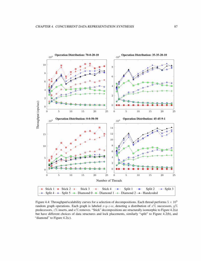
CHAPTER 4. CONCURRENT DATA REPRESENTATION SYNTHESIS 87
0 5 10 15 20 25
0
2
4
6
8
10
·103Operation Distribution: 70-0-20-10
0 5 10 15 20 25
0
2
4
6
8
·103Operation Distribution: 35-35-20-10
0 5 10 15 20 25
0
5
10
15
·103Operation Distribution: 0-0-50-50
0 5 10 15 20 25
0
2
4
6
8
10
12
14
·103Operation Distribution: 45-45-9-1
Thro
ughp
ut(o
ps/s
ec)
Number of Threads
Stick 1 Stick 2 Stick 3 Stick 4 Split 1 Split 2 Split 3Split 4 Split 5 Diamond 0 Diamond 1 Diamond 2 Handcoded
Figure 4.4: Throughput/scalability curves for a selection of decompositions. Each thread performs 5⇥ 10
5
random graph operations. Each graph is labeled x-y-z-w, denoting a distribution of x% successors, y%predecessors, z% inserts, and w% removes. “Stick” decompositions are structurally isomorphic to Figure 4.2(a)but have different choices of data structures and lock placements, similarly “split” to Figure 4.2(b), and“diamond” to Figure 4.2(c).

CHAPTER 4. CONCURRENT DATA REPRESENTATION SYNTHESIS 88
4.5.2 Graph Benchmark
We first evaluate the generated code using a synthetic benchmark modeled after the methodology of Herlihyet al. [2006] for comparing concurrent map implementations, extended to the more general context of a relation.We fix a particular relational specification, together with a set of relational operations. For any given choice ofdecomposition, the benchmark uses k identical threads that operate on a single shared relation. Starting from aninitially empty relation, each thread executes 5⇥10
5 randomly chosen operations. We plot the total throughputof all threads in operations per second against the number of threads to obtain a throughput-scalability curve.By varying the distribution of relational operations we can evaluate the performance of the relation underdifferent workloads.
For our benchmarks we use the directed graph relation described in Section 4.3.2, together with fourrelational operations, namely find successors, find predecessors, insert edge, and remove edge. The findsuccessor operation chooses a random src value and queries the relation for the set of all dst ,weight pairscorresponding to that src. The find predecessor operation is similar but chooses a random dst and queries forsrc,weight pairs. The insert edge operation chooses a random src, dst ,weight triple to insert into the relation;to ensure that the relation’s functional dependency is not violated we use the compare-and-set functionality ofthe insert operation to check that no existing edge shares the same src, dst parameters. Finally the removeoperation chooses a random (src, dst) tuple and removes the corresponding edge, if present.
We performed our experiments on a machine with two six-core 3.33Ghz Intel X5680 Xeon CPUs, eachwith 12Mb of L3 cache, and 48Gb memory in total. Hyperthreading was enabled for a total of 24 hardwarethread contexts. All benchmarks were run on a OpenJDK 6b20 Java virtual machine in server mode, with a4Gb initial and maximum heap size. We repeated each experiment 8 times within the same process, with a fullgarbage collection between runs. We discarded the results of the first 3 runs to allow the JIT compiler time towarm up; the reported values are the average of the last 5 runs.
Figure 4.4 presents throughput-scalability curves for a selection of decompositions. We generated 448variants of the three decomposition structures shown in Figure 4.2 using the autotuner, varying the choice oflock placement, lock striping factor (chosen for simplicity to be either 1 or 1024), and selection of containersfrom the options ConcurrentHashMap, ConcurrentSkipListMap, HashMap, and TreeMap. For clarity ofpresentation we selected 12 representative decompositions that cover a spectrum of different performance levelsacross the 4 benchmarks; we compare the performance of both the automatically generated implementationsand a hand-written implementation.
One obvious feature of the results is that the “stick” decompositions, which are variants of the decomposi-tion shown in Figure 4.2(a), perform relatively well for the two workloads (70-0-20-10 and 0-0-50-50) thatconsist only of successor, insert, and remove operations. For the workloads that include finding predecessors(35-35-20-10 and 45-45-9-1), “split” (Figure 4.2(b)) and “diamond” (Figure 4.2(c)) perform far better. Findingsuccessors in a stick decomposition is much more efficient than finding predecessors, which requires iteratingover all edges in the graph.
Coarsely-locked data structures scale poorly; three of the decompositions shown in the graph (Stick 1,

CHAPTER 4. CONCURRENT DATA REPRESENTATION SYNTHESIS 89
Split 1, Diamond 1) use a single coarse lock to protect the entire decomposition; each container uses a coarselylocked HashMap to represent the top level of edges in the decomposition, and a TreeMap to represent thesecond level of edges. Another decomposition (Split 2) uses striped locks and concurrent maps on the leftside of the decomposition (⇢u, uw, wx), but uses a single coarse lock to protect the other edges of the graph,leading to similarly poor performance.
Sticks 2, 3, 4 use a striped lock at the root to protect a ConcurrentHashMap of HashMap containers,a ConcurrentHashMap of TreeMap containers, and a ConcurrentSkipListMap of HashMap containers,respectively; all scale much better than the coarsely-locked data structures.
Decompositions which do not share nodes between the two sides of the decomposition outperformdecompositions that do. For example, Split 3 and Diamond 1 both use ConcurrentHashMap containers torepresent the top-level edges and HashMap containers to represent the second level edges, differing only inthe sharing structure of the decomposition; the split decomposition performs better in most cases. Split 4is a variant of Split 3 with TreeMap containers in place of the HashMap containers. Interestingly, there isa small but consistent effect where Split 3 is the best choice for the 35-35-20-10 workload and Split 4 isbetter for the 45-45-9-1 workload. Split 5 and Diamond 2 are also similar to Split 3 and Diamond 2, exceptwith ConcurrentSkipListMap containers in place of ConcurrentHashMap containers; once again, the splitdecomposition outperforms the diamond decomposition.
The handcoded implementation (which was written before the automated experiments) is essentially Split4, and produces almost identical results; the difference in performance between the two is probably due toextra boxing in the generated code that could be eliminated with improvements to the code generator. Butclearly the automatically generated code is competitive with the hand-written code but requires much lessprogrammer effort, and unless one was willing to write many different hand-coded versions, the autotuner willbe able to find variants that outperform any single hand-written code for particular workload characteristics.
It is interesting to note that diamond decompositions outperformed split decompositions in the non-concurrent case (Section 2.5.1); the result here is reversed for two reasons. The split decomposition producesless lock contention, since a pair of transactions may query for successors and predecessors in parallel withoutinterfering with one another. Much of the benefit for sharing in the non-concurrent case came from the factthat it is possible to remove an object from the middle of an intrusive doubly-linked list in constant time. Sinceit is impossible to write such intrusive containers in a generic fashion in the Java type system, we do not gainthe advantage of more efficient removals from shared nodes.
The prominent decrease in throughput evident in Figure 4.4 when increasing from 6 to 8 threads is anartifact of the thread scheduler and the memory hierarchy of the test machine. The test machine has twosix-core CPUs, each with two hardware contexts per core. The benchmark harness schedules up to the first sixthreads on different cores of the same CPU, sharing a common on-chip L3 cache. The harness schedules thenext six threads on the second CPU; when threads are split across two CPUs they must communicate via theprocessor interconnect, rather than via a shared on-chip cache. Communication off-chip is substantially slowerthan on-chip communication, producing the “notch” in the graph.

CHAPTER 4. CONCURRENT DATA REPRESENTATION SYNTHESIS 90
Overall the experiments show the benefits of automatic synthesis of both data structures and synchronization:sophisticated implementations competitive with hand written code can be produced at much lower cost inprogrammer effort, while at the same time providing guarantees about the correctness of the implementationof the high-level concurrent relational program.
4.5.3 Concurrent Cache Benchmark
In this section we apply concurrent data representation synthesis to a concurrent cache benchmark. The cachebenchmark is based on the non-concurrent examples described in Section 2.5.2, all of which use relations toimplement variants on a cache.
The benchmark models a cache as a relation with three integer-valued columns key , value and refCount .The relation satisfies a functional dependency key ! value, refCount . Each tuple in the relation is a mappingfrom a distinct integer key to an integer value. Every tuple also has an associated reference count refCount ,which is the number of active users of a particular entry in the cache. Entries with non-zero reference countsare still in use and cannot be evicted from the cache; conversely entries with zero reference counts have noactive users and are candidates for eviction.
The cache provides three operations, implemented by the code in Figure 4.5:
• Operation getReference(key, makeValue) looks up the cache entry associated a particular key. If thekey is already present, then its reference count is incremented, and the existing value associated with thekey is returned. If the key is absent, then function makeValue(key) is invoked to construct a new valuefor the key, which is then inserted into the cache with an initial reference count of 1.
• Operation putReference(key) decrements the reference count associated with key. If the key is notpresent or already has a zero reference count the operation leaves the cache unchanged.
• Operation evict() evicts entries with a zero reference count from the cache. Eviction is performed inLeast-Recently-Used (LRU) order.
The implementation in Figure 4.5 uses the relational interface generated by the compiler, which is shown inFigure 4.6. While each of the relational operations generated by the compiler is individually atomic, each cacheoperation performs multiple relational operations, so the code must guard against concurrent modificationsfrom other threads between relational operations. Both the getReference and putReference operations arestructured as loops containing a pair of relational operations: a query to find the existing data associated with akey, and an insert or an update to update that data. The insert or update double-checks the data returned bythe query operator; if an inconsistency is detected between the query and the subsequent update the cacheoperation is restarted. The evict operation uses a query operation to find all keys with a zero reference count.The subsequent removal operation double-checks that the reference count of each key is still zero; if not, thenthe key is not evicted from the cache.
We evaluate the effect of different concurrent decompositions on the performance of the cache using amethodology similar to that of Section 4.5.2. For any given choice of decomposition, the benchmark uses k
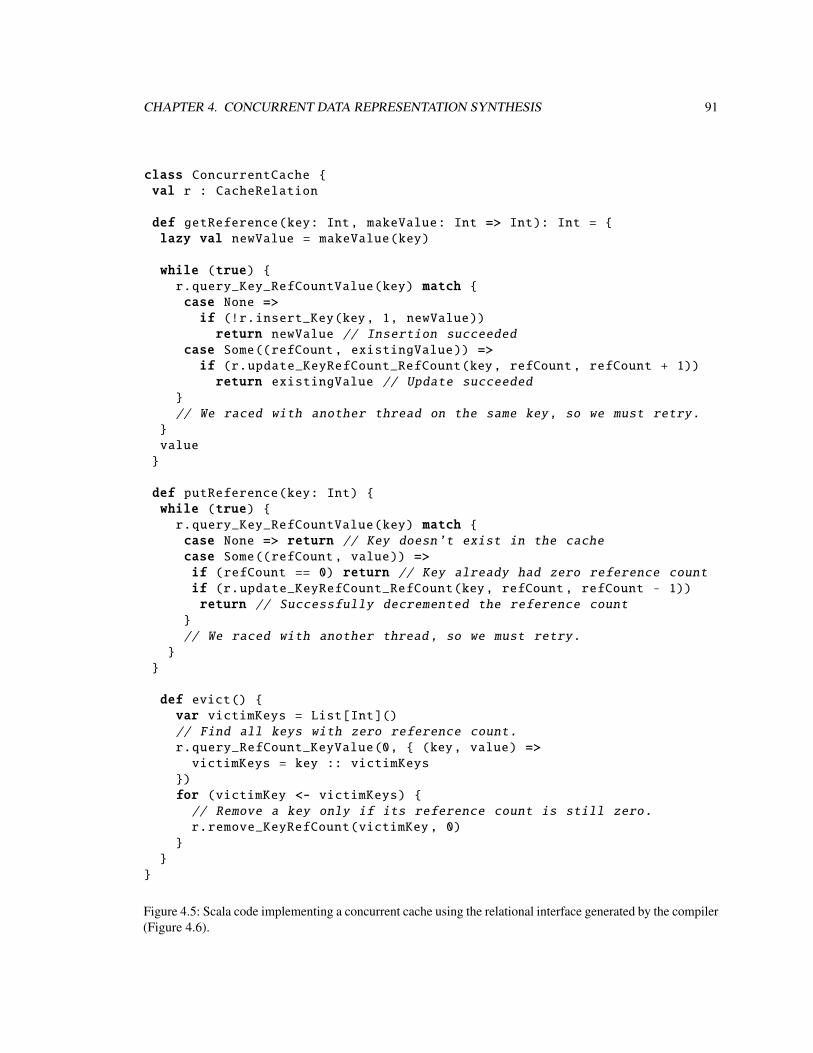
CHAPTER 4. CONCURRENT DATA REPRESENTATION SYNTHESIS 91
class ConcurrentCache {val r : CacheRelation
def getReference(key: Int, makeValue: Int => Int): Int = {lazy val newValue = makeValue(key)
while (true) {r.query_Key_RefCountValue(key) match {case None =>if (!r.insert_Key(key, 1, newValue))return newValue // Insertion succeeded
case Some((refCount , existingValue)) =>if (r.update_KeyRefCount_RefCount(key, refCount, refCount + 1))return existingValue // Update succeeded
}// We raced with another thread on the same key, so we must retry.
}value}
def putReference(key: Int) {while (true) {r.query_Key_RefCountValue(key) match {case None => return // Key doesn’t exist in the cachecase Some((refCount , value)) =>if (refCount == 0) return // Key already had zero reference countif (r.update_KeyRefCount_RefCount(key, refCount, refCount - 1))return // Successfully decremented the reference count
}// We raced with another thread, so we must retry.
}}
def evict() {var victimKeys = List[Int]()// Find all keys with zero reference count.
r.query_RefCount_KeyValue(0, { (key, value) =>victimKeys = key :: victimKeys
})for (victimKey <- victimKeys) {// Remove a key only if its reference count is still zero.
r.remove_KeyRefCount(victimKey , 0)}
}}
Figure 4.5: Scala code implementing a concurrent cache using the relational interface generated by the compiler(Figure 4.6).

CHAPTER 4. CONCURRENT DATA REPRESENTATION SYNTHESIS 92
trait CacheRelation {// Insert a new tuple into the relation , if no tuple with the same
// key already exists. Returns true if the tuple already exists.
def insert_Key(key: Int, refCount: Int, value: Int): Boolean
// Return the (refCount , value) tuple associated with a key, if any.
def query_Key_RefCountValue(key: Int): Option[(Int, Int)]
// Return the (key, value) fields of all tuples with a given refCount ,
// in Least-Recently -Used order.
def query_RefCount_KeyValue(refCount: Int,yieldFn: (Int, Int) => Unit): Unit
// Update the tuple matching key and refCount , setting the reference
// count to updRefCount. Returns true if the update was succesful.
def update_KeyRefCount_RefCount(key: Int, refCount: Int,updRefCount: Int): Boolean
// Remove the tuple with a given key and refCount , if any.
def remove_KeyRefCount(key: Int, refCount: Int): Unit}
Figure 4.6: The interface to the concurrent cache relation generated by the compiler, edited for clarity and withcomments added.
identical threads that operate on a single shared relation. Starting from an initially empty relation, each threadexecutes 5⇥ 10
4 randomly chosen cache operations. We plot the total throughput of all threads in operationsper second against the number of threads to obtain a throughput-scalability curve.
Figure 4.7(a) shows the decomposition used for the concurrent cache experiment. Each instance of nodew corresponds to an entry in the cache. There are two paths to any instance of w. Edge ⇢w maps a key tothe corresponding instance of node w. Alternatively, edge ⇢u maps a refCount to an instance of node u
corresponding to the subrelation containing entries with that reference count. For any given reference countedge uw maps each key to the corresponding instance of node w. The edge uw is annotated [LRU], whichdenotes that a scan over instances edge uw must return its results in Least-Recently-Used order.
Figure 4.8(a) presents throughput-scalability curves for the 44 variants of the decomposition in Figure 4.7(a)generated by the autotuner. The autotuner varies the choice of lock placement, lock striping factor (chosenfor simplicity to be either 1 or 1024), and selection of containers from the options ConcurrentHashMap,ConcurrentSkipListMap, HashMap, TreeMap, and a Scala DoubleLinkedList.
We describe two of the more interesting decompositions in detail. Both decompositions represent edge uwusing a DoubleLinkedList since, of the available containers, it is the only container capable of maintainingan LRU order. The decomposition labeled “ ” uses a HashMap for edges ⇢w and ⇢u, and protects everythingwith a single coarse-grained lock at the root. This decomposition performs best in the single-threaded case;

CHAPTER 4. CONCURRENT DATA REPRESENTATION SYNTHESIS 93
(a)⇢
w
u
key
refCount
key [LRU]
key , refCount , value
(b)⇢
w
u
v
key
key (mod N )
refCount
key [LRU]
key , refCount , value
Figure 4.7: Concurrent decompositions for the cache benchmark. Decomposition (a) uses a single list of keysin Least-Recently-Used order for each reference count value, whereas decomposition (b) partitions the keyspace into N partitions and uses a separate LRU list for each partition/reference count pair.
the addition of more threads only reduces performance due to lock contention. Decomposition “ ” uses aConcurrentHashMap for edges ⇢w and ⇢u, together with a lock striped by key at the root to protect instancesof edge ⇢w, and another striped lock striped by refCount at the root to protect instances of edges ⇢u. Edgeuw is protected by a lock at u, and each instance of node w has its own lock to protect the associated singletonfields. This decomposition has relatively good performance under high contention, but mediocre performancein the single-threaded case.
No variant of the decomposition shown in Figure 4.7(a) scales well, largely because every operationcontends on the locks that protect the LRU list of keys associated with each reference count. Maintaining astrict Least-Recently-Used order requires that threads agree on the observed order of cache operations, limitingparallelism.
To allow more concurrency between transactions, we altered the benchmark to relax the LRU orderingrequirement. Figure 4.7(b) shows a revised decomposition, which approximates a per-reference count LRU listby splitting the key space into a N stripes and using a separate LRU list for each (here we choose N = 1024).Although the revised decomposition no longer maintains a precise LRU order, splitting the list allows operationson the same reference count value but on different key stripes to proceed in parallel without contending on thesame lock. Figure 4.8(b) shows the results for the 162 variants of the decomposition in Figure 4.7(b) generatedby the autotuner; we describe just three in detail.
Once again, all decompositions use a DoubleLinkedList for edge vw due to the need to maintain anLRU order. Decomposition “ ” uses HashMaps to represent all of the other edges, and protects the entiredecomposition with a single coarse-grained lock at the root. This decomposition performs relatively poorlyeven in the single-threaded case, probably due to the extra overhead of maintaining additional data structuresas compared to decomposition “ ”.
Decomposition “ ” uses ConcurrentSkipListMaps to implement edges ⇢w and ⇢u, and a TreeMapto implement edge uv. A striped lock at the root indexed by key protects edge ⇢w, whereas another stripedlock at the root indexed by key (mod N) protects edges ⇢u, uv, and vw. Node w has its own lock to protect

CHAPTER 4. CONCURRENT DATA REPRESENTATION SYNTHESIS 94
0 5 10 15 20 25
0
0.2
0.4
0.6
0.8
1
1.2
1.4
·103(a) Coarse LRU Lists
0 5 10 15 20 25
0
0.2
0.4
0.6
0.8
1
1.2
1.4
·103(b) Striped LRU Lists
Thro
ughp
ut(o
ps/s
ec)
Number of Threads
Figure 4.8: Throughput/scalability curves for a selection of concurrent cache decompositions. Each threadperforms 5 ⇥ 10
4 random graph operations, with a distribution of 70% get reference operations, 28% putreference operations, and 2% eviction operations. The decompositions in the left graph use a single Least-Recently-Used list per reference count value, whereas the decompositions in the right graph approximate LRUorder by using separate lists for different parts of the key space within each reference count value.
the associated singleton fields. Decomposition “ ” is similar, but uses ConcurrentHashMap in place ofConcurrentSkipListMap, and HashMap in place of TreeMap. Both decompositions have good scalabilitycharacteristics; in particular both perform better under contention than any of the decompositions with a singleLRU list.
There are several ways to optimize the generated code which we hope to explore in future work. Firstly,all of the cache operations add or remove nodes to LRU lists. However, since Scala lacks generic intrusivedata structures, removing a node from the middle of an LRU list takes time linear in the size of the list. If wewere to extend the compiler to emit some form of intrusive linked list, we could remove linear time algorithmsfrom the getReference and putReference implementations. Secondly, the decomposition maintains a LRUlist for each reference count; it is however only necessary to maintain a LRU list just for those nodes withreference count zero. If we were to extend the compiler to support such partial data structures, then we couldavoid many unnecessary list updates for nodes with non-zero reference counts.
Finally, each of the cache operations performs multiple relational operations in succession. Since thecompiler compiles each relational operation in isolation, invoking sequences of relational operations oftenleads to redundant work between operations. In future work we hope to extend our compiler to handle a largertransaction language, rather than just a compiling a single operation at a time, allowing this redundant work tobe optimized away.

CHAPTER 4. CONCURRENT DATA REPRESENTATION SYNTHESIS 95
4.6 Discussion and Related Work
Simultaneously with and independently from our work, Manevich et al. [2012] have investigated synthesizingconcurrent graph representations from a relational description. Their approach is similar in many ways, butdiffers particularly in how abstract and concrete synchronization are used to ensure safety and serializability oftransactions. The logical locks of our concurrent decomposition language correspond to a class of abstractlocks (in their terminology). Our lock placements, which describe how to map logical locks onto a particularconcrete implementation, do not have a counterpart in their proposal. We implement concrete synchronizationboth by leveraging the safety and consistency properties of concurrent containers, and by placing restrictionson the choice of lock placement that only permit concurrent access to a container if such access is safe andlinearizable. In their proposal abstract synchronization is implemented as a separate table of abstract locks, itis the responsibility of individual containers to ensure concrete safety and linearizability.
The closest previous literature to our work in spirit is Paraglider [Vechev and Yahav, 2008], which providessemi-automatic assistance in synthesizing low-level concurrent algorithms and data structures. Paragliderfocuses on the correct implementation of a single concurrent data structure, while our work is about assemblingmultiple concurrent and non-concurrent data structures into more complex abstractions. Thus, Paraglider iscomplementary to our approach, and we could extend our menu of concurrent building blocks with Paraglider-generated components.
Our system can be viewed as implementing a pessimistic software transactional memory [Shavit andTouitou, 1997]. Future extensions of our work could synthesize optimistic concurrency control primitivesin addition to pessimistic locks. Unlike traditional software transactional memory systems, which performon-line dynamic analysis to determine the read and write sets of transactions, our system performs much ofthe same analysis statically, resulting in run-time code with considerably lower overhead. Furthermore, ourapproach is able to automatically change the data structures and granularity of locking used to improve overallperformance. It is also worth noting that speculative locking was first introduced in the context of advancedsoftware transactional memory systems [Bronson et al., 2010a].

Chapter 5
Conclusions
This dissertation proposes a new approach for specifying combinations of data structures with complex sharingin a manner that is both declarative and results in provably correct code.
We describe a scheme for synthesizing efficient low-level data representations from abstract relationaldescriptions of data. In our approach programmers describe and manipulate data at a high level as relations,and it is the task of the compiler to generate implementations of the various relational operations specialized toa particular representation.
We propose a novel decomposition language, which specifies how relations should be mapped to low-levelphysical implementations, assembled from a library of primitive container data structures. The decompositionlanguage provides a new way to specify high-level heap invariants that are difficult or impossible to expressusing standard data abstraction or heap-analysis techniques. We describe adequacy conditions that ensure adecomposition faithfully represents a relation.
Decompositions can be combined with locks to describe a wide range of concurrent representations ofdata. We introduce the idea of a lock placement: such diverse concepts as lock granularity, speculative locks,lock splitting and merging, and dynamically changing lock assignments can all be understood as examples of alock placement that maps each heap field to a lock that guards it. We have also identified the key concept of astable set of mutually supporting locks and heap facts, where the set of locks protect the heap facts and theset of heap facts preserve the lock placement. We have used these two concepts to develop a series of proofsystems for showing that transactions are well-locked and therefore serializable, applying these technique toflat heaps, tree-structured heaps, and finally decompositions.
We describe how to synthesize efficient low-level implementations of relational queries and updates,specialized to a particular decomposition. Key to our approach is a query planner that chooses an efficientexecution plan for each query or mutation. We show that queries and updates are sound, that is, the implemen-tation generated by our compiler for each query or mutation faithfully implements its relational specification.We extend query planning to concurrent relations; the concurrent query planner ensures that queries take thecorrect locks in the correct order to guarantee serializability and deadlock-freedom.
96

CHAPTER 5. CONCLUSIONS 97
A programmer may not know the best decomposition for a particular relation. We describe an autotuner,which given a relational specification and a performance metric, such as a benchmark, finds the decompositionwith the best combination of data structures for that query load. We extend the autotuner to support concurrency;the concurrent autotuner finds the decomposition with the combination of data structures and lock placementthat produces the best performance. Exploring different choices of data structures and locking strategiesis extremely difficult in hand-written code, since writing concurrent data structure code is a difficult anderror-prone process.
Finally we describe our experience with two different implementations of data representation synthesis.We describe a non-concurrent compiler which takes an input a relation and its decomposition and generatesC++ code implementing the relation, which is easily incorporated into existing systems. We also describe aseparate concurrent implementation, which converts a decomposition incorporating a lock placement into aScala implementation. We demonstrate that different choices of decomposition have very different performancecharacteristics. We incorporate synthesis into a variety of real systems, in each case leading to code that issimpler, correct by construction, and comparable in performance.

Bibliography
Daniel Abadi, Samuel Madden, and Miguel Ferreira. Integrating compression and execution in column-oriented database systems. In Proceedings of the ACM SIGMOD International Conference on Managementof Data, pages 671–682, New York, NY, USA, 2006. ACM. ISBN 1-59593-434-0. doi: 10.1145/1142473.1142548.
Daniel J. Abadi, Samuel R. Madden, and Nabil Hachem. Column-stores vs. row-stores: How different arethey really? In Proceedings of the ACM SIGMOD International Conference on Management of Data, pages967–980, New York, NY, USA, 2008. ACM. ISBN 978-1-60558-102-6. doi: 10.1145/1376616.1376712.
Nawaaz Ahmed, Nikolay Mateev, Keshav Pingali, and Paul Stodghill. A framework for sparse matrix codesynthesis from high-level specifications. In Supercomputing, page 58. IEEE Computer Society, November2000. doi: 10.1109/SC.2000.10033.
Lars Ole Andersen. Program Analysis and Specialization for the C Programming Language. Ph.D. thesis,DIKU, University of Copenhagen, Denmark, 1994.
Hagit Attiya, G. Ramalingam, and Noam Rinetzky. Sequential verification of serializability. In Proceedings ofthe ACM SIGPLAN-SIGACT Symposium on Principles of Programming Languages (POPL), pages 31–42,New York, NY, USA, 2010. ACM. ISBN 978-1-60558-479-9. doi: 10.1145/1706299.1706305.
Don Batory and Jeff Thomas. P2: A lightweight DBMS generator. Journal of Intelligent Information Systems,9:107–123, 1997. ISSN 0925-9902. doi: 10.1023/A:1008617930959.
Don Batory, Gang Chen, Eric Robertson, and Tao Wang. Design wizards and visual programming environmentsfor GenVoca generators. IEEE Transactions on Software Engineering, 26(5):441–452, May 2000. ISSN0098-5589. doi: 10.1109/32.846301.
J. Baulier, P. Bohannon, S. Gogate, C. Gupta, and S. Haldar. DataBlitz storage manager: Main-memory databaseperformance for critical applications. In Proceedings of the ACM SIGMOD International Conference onManagement of Data, pages 519–520, New York, NY, USA, 1999. ACM. ISBN 1-58113-084-8. doi:10.1145/304182.304239.
98

BIBLIOGRAPHY 99
Catriel Beeri, Ronald Fagin, and John H. Howard. A complete axiomatization for functional and multivalueddependencies in database relations. In Proceedings of the ACM SIGMOD International Conference onManagement of Data, pages 47–61, New York, NY, USA, 1977. ACM. doi: 10.1145/509404.509414.
Josh Berdine, Cristiano Calcagno, and Peter O’Hearn. Symbolic execution with separation logic. In KwangkeunYi, editor, Programming Languages and Systems, volume 3780 of Lecture Notes in Computer Science, pages52–68. Springer Berlin / Heidelberg, 2005. ISBN 978-3-540-29735-2. doi: 10.1007/11575467_5.
Josh Berdine, Cristiano Calgano, Byron Cook, Dino Distefano, Peter W. O’Hearn, Thomas Wies, and HongseokYang. Shape analysis for composite data structures. In Proceedings of Computer Aided Verification (CAV),volume 4590 of Lecture Notes in Computer Science, pages 178–192. Springer Berlin / Heidelberg, 2007.doi: 10.1007/978-3-540-73368-3_22.
Gavin Bierman and Alisdair Wren. First-class relationships in an object-oriented language. In Proceedingsof the European Conference on Object-Oriented Programming (ECOOP), volume 3586 of LNCS, pages262–286. Springer Berlin / Heidelberg, 2005. doi: 10.1007/11531142_12.
Cui Bin. Indexing for Efficient Main Memory Processing. Ph.D. thesis, National University of Singapore,2003.
Lars Birkedal, Noah Torp-Smith, and John C. Reynolds. Local reasoning about a copying garbage collector. InProceedings of the ACM SIGPLAN-SIGACT Symposium on Principles of Programming Languages (POPL),pages 220–231. ACM, 2004. doi: 10.1145/964001.964020.
Peter Boncz, Martin Zukowski, and Niels Nes. MonetDB/X100: Hyper-pipelining query execution. InProceedings of the Conference on Innovative Data Systems Research (CIDR), pages 225–237. VLDB, 2005.URL http://www.cidrdb.org/cidr2005/papers/P19.pdf.
Peter A. Boncz and Martin L. Kersten. MIL primitives for querying a fragmented world. The VLDB Journal,8:101–119, 1999. ISSN 1066-8888. doi: 10.1007/s007780050076.
Boost. Boost C++ libraries, 2010. URL http://www.boost.org/.
Richard Bornat, Cristiano Calcagno, and Peter O’Hearn. Local reasoning, separation, and aliasing. InProceedings of the 2nd Workshop on Semantics, Program Analysis, and Compute Environments forMemory Management (SPACE), 2004. URL http://www.diku.dk/topps/space2004/space_final/bornat-calcagno-ohearn.pdf.
Nathan G. Bronson. Composable Operations on High-Performance Concurrent Collections. Ph.D. thesis,Stanford University, 2011.
Nathan G. Bronson, Jared Casper, Hassan Chafi, and Kunle Olukotun. Transactional predication: High-performance concurrent sets and maps for STM. In Proceeding of the 29th ACM SIGACT-SIGOPS

BIBLIOGRAPHY 100
Symposium on Principles of Distributed Computing (PODC), pages 6–15, New York, NY, USA, 2010a.ACM. ISBN 978-1-60558-888-9. doi: 10.1145/1835698.1835703.
Nathan G. Bronson, Jared Casper, Hassan Chafi, and Kunle Olukotun. A practical concurrent binary searchtree. In Proceedings of the 15th ACM SIGPLAN Symposium on Principles and Practice of ParallelProgramming (PPoPP), pages 257–268, New York, NY, USA, 2010b. ACM. ISBN 978-1-60558-877-3.doi: 10.1145/1693453.1693488.
Jiazhen Cai and Robert A. Paige. “Look ma, no hashing, and no arrays neither”. In Proceedings of the ACMSIGPLAN-SIGACT Symposium on Principles of Programming Languages (POPL), pages 143–154, NewYork, NY, USA, 1991. ACM. ISBN 0-89791-419-8. doi: 10.1145/99583.99605.
Cristiano Calcagno, Dino Distefano, Peter O’Hearn, and Hongseok Yang. Compositional shape analysisby means of bi-abduction. In Proceedings of the ACM SIGPLAN-SIGACT Symposium on Principles ofProgramming Languages (POPL). ACM, 2009. doi: 10.1145/1480881.1480917.
David R. Chase, Mark Wegman, and F. Kenneth Zadeck. Analysis of pointers and structures. In Proceedingsof the ACM SIGPLAN Conference on Programming Language Design and Implementation (PLDI), pages296–310. ACM, 1990. ISBN 0-89791-364-7. doi: 10.1145/93542.93585.
Shaunak Chatterjee, Shuvendu Lahiri, Shaz Qadeer, and Zvonimir Rakamaric. A reachability predicate foranalyzing low-level software. In Orna Grumberg and Michael Huth, editors, Tools and Algorithms for theConstruction and Analysis of Systems, volume 4424 of Lecture Notes in Computer Science, pages 19–33.Springer Berlin / Heidelberg, 2007. ISBN 978-3-540-71208-4. doi: 10.1007/978-3-540-71209-1_4.
Surajit Chaudhuri and Vivek R. Narasayya. An efficient cost-driven index selection tool for Microsoft SQLServer. In Proceedings of the International Conference on Very Large Databases (VLDB), pages 146–155,San Francisco, CA, USA, 1997. Morgan Kaufmann Publishers. ISBN 1-55860-470-7.
Sigmund Cherem, Trishul Chilimbi, and Sumit Gulwani. Inferring locks for atomic sections. In Proceedingsof the ACM SIGPLAN Conference on Programming Language Design and Implementation (PLDI), pages304–315, New York, NY, USA, 2008. ACM. ISBN 978-1-59593-860-2. doi: 10.1145/1375581.1375619.
Adam Chlipala, Gregory Malecha, Greg Morrisett, Avraham Shinnar, and Ryan Wisnesky. Effective interactiveproofs for higher-order imperative programs. In Proceedings of the 14th ACM SIGPLAN InternationalConference on Functional Programming, pages 79–90, New York, NY, USA, 2009. ACM. ISBN 978-1-60558-332-7. doi: 10.1145/1596550.1596565.
Edgar F. Codd. A relational model of data for large shared data banks. Communications of the ACM, 13(6):377–387, 1970. ISSN 0001-0782. doi: 10.1145/362384.362685.
Donald Cohen and Neil Campbell. Automating relational operations on data structures. IEEE Software, 10(3):53–60, May 1993. doi: 10.1109/52.210604.

BIBLIOGRAPHY 101
Dave Cunningham, Khilan Gudka, and Susan Eisenbach. Keep off the grass: Locking the right path foratomicity. In Laurie Hendren, editor, Compiler Construction, volume 4959 of Lecture Notes in ComputerScience, pages 276–290. Springer Berlin / Heidelberg, 2008. ISBN 978-3-540-78790-7. doi: 10.1007/978-3-540-78791-4_19.
Manuvir Das. Unification-based pointer analysis with directional assignments. In Proceedings of the ACMSIGPLAN Conference on Programming Language Design and Implementation (PLDI), pages 35–46, NewYork, NY, USA, 2000. ACM. ISBN 1-58113-199-2. doi: 10.1145/349299.349309.
Jyotirmoy Deshmukh, G. Ramalingam, Venkatesh-Prasad Ranganath, and Kapil Vaswani. Logical concurrencycontrol from sequential proofs. In Programming Languages and Systems, volume 6012 of LNCS, pages 226–245. Springer Berlin / Heidelberg, 2010. ISBN 978-3-642-11956-9. doi: 10.1007/978-3-642-11957-6_13.
Alain Deutsch. A storeless model of aliasing and its abstractions using finite representations of right-regularequivalence relations. In Proceedings of the International Conference of Computer Languages, pages 2–13,Apr 1992. doi: 10.1109/ICCL.1992.185463.
Robert B. K. Dewar, Arthur Grand, Ssu-Cheng Liu, Jacob T. Schwartz, and Edmond Schonberg. Programmingby refinement, as exemplified by the SETL representation sublanguage. ACM Transactions on ProgrammingLanguages and Systems (TOPLAS), 1(1):27–49, January 1979. ISSN 0164-0925. doi: 10.1145/357062.357064.
David J. DeWitt, Randy H. Katz, Frank Olken, Leonard D. Shapiro, Michael R. Stonebraker, and David A.Wood. Implementation techniques for main memory database systems. In Proceedings of the ACM SIGMODInternational Conference on Management of Data, SIGMOD, pages 1–8, New York, NY, USA, 1984. ACM.ISBN 0-89791-128-8. doi: 10.1145/602259.602261.
Pedro C. Diniz and Martin C. Rinard. Lock coarsening: Eliminating lock overhead in automatically parallelizedobject-based programs. Journal of Parallel and Distributed Computing, 49(2):218–244, 1998. ISSN 0743-7315. doi: 10.1006/jpdc.1998.1441.
Dino Distefano, Peter O’Hearn, and Hongseok Yang. A local shape analysis based on separation logic. InTools and Algorithms for the Construction and Analysis of Systems, volume 3920 of Lecture Notes inComputer Science, pages 287–302. Springer Berlin / Heidelberg, 2006. ISBN 978-3-540-33056-1. doi:10.1007/11691372_19.
Maryam Emami, Rakesh Ghiya, and Laurie J. Hendren. Context-sensitive interprocedural points-to analysisin the presence of function pointers. In Proceedings of the ACM SIGPLAN Conference on ProgrammingLanguage Design and Implementation (PLDI), pages 242–256, New York, NY, USA, 1994. ACM. ISBN0-89791-662-X. doi: 10.1145/178243.178264.

BIBLIOGRAPHY 102
Michael Emmi, Jeffrey S. Fischer, Ranjit Jhala, and Rupak Majumdar. Lock allocation. In Proceedings ofthe 34th ACM SIGPLAN-SIGACT Symposium on Principles of Programming Languages (POPL), pages291–296, New York, NY, USA, 2007. ACM. ISBN 1-59593-575-4. doi: 10.1145/1190216.1190260.
K. P. Eswaran, J. N. Gray, R. A. Lorie, and I. L. Traiger. The notions of consistency and predicate locks ina database system. Communications of the ACM, 19:624–633, November 1976. ISSN 0001-0782. doi:10.1145/360363.360369.
Manuel Fähndrich and K. Rustan M. Leino. Heap monotonic typestates. In Proceedings of the InternationalWorkshop on Alias Confinement and Ownership, July 2003.
Manuel Fähndrich, Jakob Rehof, and Manuvir Das. Scalable context-sensitive flow analysis using instantiationconstraints. In Proceedings of the ACM SIGPLAN Conference on Programming Language Design andImplementation (PLDI), pages 253–263, New York, NY, USA, 2000. ACM. ISBN 1-58113-199-2. doi:10.1145/349299.349332.
Hector Garcia-Molina and Kenneth Salem. Main memory database systems: An overview. Knowledgeand Data Engineering, IEEE Transactions on, 4(6):509–516, December 1992. ISSN 1041-4347. doi:10.1109/69.180602.
Guy Golan-Gueta, Nathan Bronson, Alex Aiken, G. Ramalingam, Mooly Sagiv, and Eran Yahav. Automaticfine-grain locking using shape properties. In Proceedings of the ACM SIGPLAN Conference on Object-Oriented Programming Systems, Languages, and Applications (OOPSLA), 2011.
Alexey Gotsman, Josh Berdine, and Byron Cook. Interprocedural shape analysis with separated heap abstrac-tions. In Static Analysis, volume 4134 of Lecture Notes in Computer Science, pages 240–260. SpringerBerlin / Heidelberg, 2006. ISBN 978-3-540-37756-6. doi: 10.1007/11823230_16.
Alexey Gotsman, Josh Berdine, Byron Cook, Noam Rinetzky, and Mooly Sagiv. Local reasoning for storablelocks and threads. In Proceedings of the Asian Symposium on Programming Languages and Systems(APLAS), volume 4807 of Lecture Notes in Computer Science, pages 19–37. Springer Berlin / Heidelberg,2007. ISBN 978-3-540-76636-0. doi: 10.1007/978-3-540-76637-7_3.
Sumit Gulwani and Ashish Tiwari. An abstract domain for analyzing heap-manipulating low-level software. InWerner Damm and Holger Hermanns, editors, Proceedings of Computer Aided Verification (CAV), volume4590 of Lecture Notes in Computer Science, pages 379–392. Springer Berlin / Heidelberg, 2007. ISBN978-3-540-73367-6. doi: 10.1007/978-3-540-73368-3_42.
Bolei Guo, Neil Vachharajani, and David I. August. Shape analysis with inductive recursion synthesis. InProceedings of the ACM SIGPLAN Conference on Programming Language Design and Implementation(PLDI), pages 256–265, New York, NY, USA, 2007. ACM. ISBN 978-1-59593-633-2. doi: 10.1145/1250734.1250764.

BIBLIOGRAPHY 103
Brian Hackett and Radu Rugina. Region-based shape analysis with tracked locations. In Proceedings of theACM SIGPLAN-SIGACT Symposium on Principles of Programming Languages (POPL), pages 310–323,New York, NY, USA, 2005. ACM. ISBN 1-58113-830-X. doi: 10.1145/1040305.1040331.
Richard L. Halpert, Christopher J. F. Pickett, and Clark Verbrugge. Component-based lock allocation. InProceedings of the 16th International Conference on Parallel Architecture and Compilation Techniques,PACT ’07, pages 353–364, Washington, DC, USA, 2007. IEEE Computer Society. ISBN 0-7695-2944-5.doi: 10.1109/PACT.2007.23.
Peter Hawkins, Alex Aiken, Kathleen Fisher, Martin Rinard, and Mooly Sagiv. Data structure fusion. InProceedings of the Asian Symposium on Programming Languages and Systems (APLAS), volume 6461 ofLecture Notes in Computer Science, pages 204–221. Springer Berlin / Heidelberg, 2010. doi: 10.1007/978-3-642-17164-2_15.
Peter Hawkins, Alex Aiken, Kathleen Fisher, Martin Rinard, and Mooly Sagiv. Data representation synthesis. InProceedings of the 32nd ACM SIGPLAN Conference on Programming Language Design and Implementation(PLDI), pages 38–49, New York, NY, USA, 2011. ACM. ISBN 978-1-4503-0663-8. doi: 10.1145/1993498.1993504.
Peter Hawkins, Alex Aiken, Kathleen Fisher, Martin Rinard, and Mooly Sagiv. Reasoning about lock place-ments. In Programming Languages and Systems, volume 7211 of LNCS, pages 336–356. Springer Berlin /Heidelberg, 2012a. ISBN 978-3-642-28868-5. doi: 10.1007/978-3-642-28869-2_17.
Peter Hawkins, Alex Aiken, Kathleen Fisher, Martin Rinard, and Mooly Sagiv. Concurrent data representationsynthesis. In Proceedings of the 33rd ACM SIGPLAN Conference on Programming Language Design andImplementation (PLDI), New York, NY, USA, 2012b. ACM.
David L. Heine and Monica S. Lam. A practical flow-sensitive and context-sensitive C and C++ memoryleak detector. In Proceedings of the ACM SIGPLAN Conference on Programming Language Design andImplementation (PLDI), pages 168–181, New York, NY, USA, 2003. ACM. ISBN 1-58113-662-5. doi:10.1145/781131.781150.
Laurie J. Hendren, Joseph Hummell, and Alexandru Nicolau. Abstractions for recursive pointer data structures:Improving the analysis and transformation of imperative programs. In Proceedings of the ACM SIGPLANConference on Programming Language Design and Implementation (PLDI), pages 249–260, New York,NY, USA, 1992. ACM. ISBN 0-89791-475-9. doi: 10.1145/143095.143138.
Maurice Herlihy, Yossi Lev, Victor Luchangco, and Nir Shavit. A provably correct scalable concurrent skiplist. In Proceedings of the Conference On Principles of Distributed Systems (OPODIS), 2006.
Maurice P. Herlihy and Jeannette M. Wing. Linearizability: A correctness condition for concurrent objects.ACM Transactions on Programming Languages and Systems (TOPLAS), 12:463–492, July 1990. ISSN0164-0925. doi: 10.1145/78969.78972.

BIBLIOGRAPHY 104
Michael Hicks, Jeffrey S. Foster, and Polyvios Pratikakis. Lock inference for atomic sections. In Workshop onLanguages, Compilers and Hardware Support for Transactional Computing, 2006.
C.B. Jones. Development methods for computer programs including a notion of interference. Ph.D. thesis,Oxford University, 1981.
Uri Juhasz, Noam Rinetzk, Arnd Poetzsch-Heffter, Mooly Sagiv, and Eran Yahav. Modular verification withshared abstractions. In International Workshop on Foundations of Object-Oriented Languages (FOOL),2009.
Nils Klarlund and Michael I. Schwartzbach. Graph types. In Proceedings of the ACM SIGPLAN-SIGACTSymposium on Principles of Programming Languages (POPL), pages 196–205, New York, NY, USA, 1993.ACM. ISBN 0-89791-560-7. doi: 10.1145/158511.158628.
Vladimir Kotlyar, Keshav Pingali, and Paul Stodghill. A relational approach to the compilation of sparsematrix programs. In Euro-Par’97 Parallel Processing, volume 1300 of Lecture Notes in Computer Science,pages 318–327. Springer Berlin / Heidelberg, 1997. doi: 10.1007/BFb0002751.
Jörg Kreiker, Helmut Seidl, and Vesal Vojdani. Shape analysis of low-level C with overlapping structures. In Ver-ification, Model Checking, and Abstract Interpretation (VMCAI), volume 5044 of Lecture Notes in ComputerScience, pages 214–230. Springer Berlin / Heidelberg, 2010. doi: 10.1007/978-3-642-11319-2_17.
Victor Kuncak, Patrick Lam, Karen Zee, and Martin Rinard. Modular pluggable analyses for data structureconsistency. IEEE Transactions on Software Engineering, 32(12):988–1005, 2006. ISSN 0098-5589. doi:10.1109/TSE.2006.125.
Viktor Kuncak, Patrick Lam, and Martin Rinard. Role analysis. In Proceedings of the ACM SIGPLAN-SIGACTSymposium on Principles of Programming Languages (POPL), pages 17–32, New York, NY, USA, 2002.ACM. ISBN 1-58113-450-9. doi: 10.1145/503272.503276.
Patrick Lam. The Hob system for verifying software design properties. Ph.D. thesis, MIT, Cambridge, MA,USA, 2007.
Patrick Lam, Viktor Kuncak, and Martin Rinard. Generalized typestate checking for data structure consistency.In Verification, Model Checking, and Abstract Interpretation (VMCAI), volume 3385 of Lecture Notes in Com-puter Science, pages 430–447. Springer Berlin / Heidelberg, 2005. doi: 10.1007/978-3-540-30579-8_28.
William Landi and Barbara G. Ryder. A safe approximate algorithm for interprocedural aliasing. In Proceedingsof the ACM SIGPLAN Conference on Programming Language Design and Implementation (PLDI), pages235–248, New York, NY, USA, 1992. ACM. ISBN 0-89791-475-9. doi: 10.1145/143095.143137.

BIBLIOGRAPHY 105
William Landi, Barbara G. Ryder, and Sean Zhang. Interprocedural modification side effect analysis withpointer aliasing. In Proceedings of the ACM SIGPLAN Conference on Programming Language Designand Implementation (PLDI), pages 56–67, New York, NY, USA, 1993. ACM. ISBN 0-89791-598-4. doi:10.1145/155090.155096.
Oukseh Lee, Hongseok Yang, and Kwangkeun Yi. Automatic verification of pointer programs using grammar-based shape analysis. In Programming Languages and Systems, volume 3444 of Lecture Notes in ComputerScience, pages 140–140. Springer Berlin / Heidelberg, 2005. ISBN 978-3-540-25435-5. doi: 10.1007/978-3-540-31987-0_10.
Oukseh Lee, Hongseok Yang, and Rasmus Petersen. Program analysis for overlaid data structures. In Proceed-ings of Computer Aided Verification (CAV), volume 6806 of Lecture Notes in Computer Science, pages 592–608. Springer Berlin / Heidelberg, 2011. ISBN 978-3-642-22109-5. doi: 10.1007/978-3-642-22110-1_48.
Tobin J. Lehman and Michael J. Carey. A study of index structures for main memory database managementsystems. In Wesley W. Chu, Georges Gardarin, Setsuo Ohsuga, and Yahiko Kambayashi, editors, Proceedingsof the 12th International Conference on Very Large Databases (VLDB), pages 294–303. Morgan Kaufmann,1986. ISBN 0-934613-18-4.
Tobin J. Lehman, Eugene J. Shekita, and Luis-Felipe Cabrera. An evaluation of Starburst’s memory residentstorage component. IEEE Transactions on Knowledge and Data Engineering, 4(6):555–566, dec 1992.ISSN 1041-4347. doi: 10.1109/69.180606.
Hongjun Lu, Yuet Yeung Ng, and Zengping Tian. T-tree or B-tree: Main memory database index structurerevisited. In Proceedings of the 11th Australasian Database Conference (ADC), pages 65–73, 2000. doi:10.1109/ADC.2000.819815.
Stephen Magill, Aleksandar Nanevski, Edmund Clarke, and Peter Lee. Inferring invariants in separation logicfor imperative list-processing programs. In 3rd SPACE Workshop, 2006.
Roman Manevich, Rashid Kaleem, and Keshav Pingali. Synthesizing concurrent relational data structures.Technical Report TR-2012-17, The University of Texas at Austin, 2012.
Mark Marron, Darko Stefanovic, Manuel Hermenegildo, and Deepak Kapur. Heap analysis in the presence ofcollection libraries. In Proceedings of the 7th ACM SIGPLAN-SIGSOFT Workshop on Program Analysisfor Software Tools and Engineering (PASTE), pages 31–36, New York, NY, USA, 2007. ACM. ISBN978-1-59593-595-3. doi: 10.1145/1251535.1251541.
Bill McCloskey, Feng Zhou, David Gay, and Eric Brewer. Autolocker: Synchronization inference for atomicsections. In Proceedings of the 33rd ACM SIGPLAN-SIGACT Symposium on Principles of ProgrammingLanguages (POPL), pages 346–358, New York, NY, USA, 2006. ACM. ISBN 1-59593-027-2. doi:10.1145/1111037.1111068.

BIBLIOGRAPHY 106
Bill McCloskey, Thomas Reps, and Mooly Sagiv. Statically inferring complex heap, array, and numericinvariants. In Static Analysis, volume 6337 of Lecture Notes in Computer Science, pages 71–99. SpringerBerlin / Heidelberg, 2011. ISBN 978-3-642-15768-4. doi: 10.1007/978-3-642-15769-1_6.
Scott McPeak and George Necula. Data structure specifications via local equality axioms. In Proceedings ofComputer Aided Verification (CAV), volume 3576 of Lecture Notes in Computer Science, pages 476–490.Springer Berlin / Heidelberg, 2005. ISBN 978-3-540-27231-1. doi: 10.1007/11513988_47.
Eric Meijer, Brian Beckman, and Gavin Bierman. LINQ: Reconciling objects, relations and XML in the .NETframework. In SIGMOD, pages 706–706, New York, NY, USA, 2006. ACM. ISBN 1-59593-434-0. doi:10.1145/1142473.1142552.
Anders Møller and Michael I. Schwartzbach. The Pointer Assertion Logic Engine. In Proceedings of the ACMSIGPLAN Conference on Programming Language Design and Implementation (PLDI), pages 221–231,New York, NY, USA, 2001. ACM. ISBN 1-58113-414-2. doi: 10.1145/378795.378851.
Mayur Naik and Alex Aiken. Conditional must not aliasing for static race detection. In Proceedings of theACM SIGPLAN-SIGACT Symposium on Principles of Programming Languages (POPL), pages 327–338.ACM, 2007. ISBN 1-59593-575-4. doi: 10.1145/1190216.1190265.
Martin Odersky, Philippe Altherr, Vincent Cremet, Iulian Dragos, Gilles Dubochet, Burak Emir, SeanMcDirmid, Stéphane Micheloud, Nikolay Mihaylov, Michel Schinz, Erik Stenman, Lex Spoon, and MatthiasZenger. An Overview of the Scala Programming Language, second edition. Technical Report LAMP-REPORT-2006-001, École Polytechnique Fédérale de Lausanne (EPFL), Lausanne, Switzerland, 2006.
Peter W. O’Hearn. Resources, concurrency, and local reasoning. Theoretical Computer Science, 375(1–3):271–307, 2007.
John Ousterhout, Parag Agrawal, David Erickson, Christos Kozyrakis, Jacob Leverich, David Mazières,Subhasish Mitra, Aravind Narayanan, Guru Parulkar, Mendel Rosenblum, Stephen M. Rumble, Eric Strat-mann, and Ryan Stutsman. The case for RAMClouds: Scalable high-performance storage entirely inDRAM. ACM SIGOPS Operating Systems Review, 43(4):92–105, January 2010. ISSN 0163-5980. doi:10.1145/1713254.1713276.
Robert Paige and Fritz Henglein. Mechanical translation of set theoretic problem specifications into efficientRAM code — a case study. Journal of Symbolic Computation, 4(2):207–232, 1987. ISSN 0747-7171. doi:10.1016/S0747-7171(87)80066-4.
Jun Rao and Kenneth A. Ross. Cache conscious indexing for decision-support in main memory. In Proceedingsof the International Conference on Very Large Databases (VLDB), pages 78–89, 1999.
Jun Rao and Kenneth A. Ross. Making B+- trees cache conscious in main memory. In Proceedings of theACM SIGMOD International Conference on Management of Data, pages 475–486, New York, NY, USA,2000. ACM. ISBN 1-58113-217-4. doi: 10.1145/342009.335449.

BIBLIOGRAPHY 107
John C. Reynolds. Separation logic: A logic for shared mutable data structures. In Proceedings of the 17thAnnual IEEE Symposium on Logic in Computer Science (LICS), pages 55–74, 2002. doi: 10.1109/LICS.2002.1029817. Invited paper.
Tom Rothamel and Yanhong A. Liu. Efficient implementation of tuple pattern based retrieval. In Proceedingsof the ACM SIGPLAN Workshop on Partial Evaluation and Program Manipulation (PEPM), pages 81–90,New York, NY, USA, 2007. ACM. ISBN 978-1-59593-620-2. doi: 10.1145/1244381.1244394.
Mooly Sagiv, Thomas Reps, and Reinhard Wilhelm. Parametric shape analysis via 3-valued logic. ACMTransactions on Programming Languages and Systems, 24(3):217–298, 2002. ISSN 0164-0925. doi:10.1145/514188.514190.
Edmond Schonberg, Jacob T. Schwartz, and Micha Sharir. Automatic data structure selection in SETL. InProceedings of the ACM SIGPLAN-SIGACT Symposium on Principles of Programming Languages (POPL),pages 197–210, New York, NY, USA, 1979. ACM. doi: 10.1145/567752.567771.
Ohad Shacham, Martin Vechev, and Eran Yahav. Chameleon: Adaptive selection of collections. In Proceedingsof the ACM SIGPLAN Conference on Programming Language Design and Implementation (PLDI), pages408–418, New York, NY, USA, 2009. ACM. ISBN 978-1-60558-392-1. doi: 10.1145/1542476.1542522.
Ohad Shacham, Nathan Bronson, Alex Aiken, Mooly Sagiv, Martin Vechev, and Eran Yahav. Testing atomicityof composed concurrent operations. In Proceedings of the ACM SIGPLAN Conference on Object-OrientedProgramming Systems, Languages, and Applications (OOPSLA), October 2011.
Nir Shavit and Dan Touitou. Software transactional memory. Distributed Computing, 10:99–116, 1997. ISSN0178-2770. doi: 10.1007/s004460050028.
Yannis Smaragdakis and Don Batory. DiSTiL: A transformation library for data structures. In Conference onDomain-Specific Languages, pages 257–271, October 1997.
Bjarne Steensgaard. Points-to analysis in almost linear time. In Proceedings of the 23rd ACM SIGPLAN-SIGACT Symposium on Principles of Programming Languages (POPL), pages 32–41, New York, NY, USA,1996. ACM. ISBN 0-89791-769-3. doi: 10.1145/237721.237727.
Michael Stonebraker, Chuck Bear, Ugur Çetintemel, Mitch Cherniack, Tingjian Ge, Nabil Hachem, StavrosHarizopoulos, John Lifter, Jennie Rogers, and Stan Zdonik. One size fits all? — Part 2: Benchmarkingresults. In Proceedings of the Conference on Innovative Data Systems Research (CIDR), pages 173–184.VLDB, 2007a. URL http://www.cidrdb.org/cidr2007/papers/cidr07p20.pdf.
Michael Stonebraker, Samuel Madden, Daniel J. Abadi, Stavros Harizopoulos, Nabil Hachem, and Pat Helland.The end of an architectural era: (It’s time for a complete rewrite). In Proceedings of the 33rd InternationalConference on Very Large Databases (VLDB), pages 1150–1160, 2007b. ISBN 978-1-59593-649-3.

BIBLIOGRAPHY 108
Mike Stonebraker, Daniel J. Abadi, Adam Batkin, Xuedong Chen, Mitch Cherniack, Miguel Ferreira, EdmondLau, Amerson Lin, Sam Madden, Elizabeth O’Neil, Pat O’Neil, Alex Rasin, Nga Tran, and Stan Zdonik.C-store: A column-oriented DBMS. In Proceedings of the 31st International Conference on Very LargeDatabases (VLDB), pages 553–564, 2005. ISBN 1-59593-154-6.
TimesTen. In-memory data management for consumer transactions: The TimesTen approach. In Proceedingsof the ACM SIGMOD International Conference on Management of Data, pages 528–529, New York, NY,USA, 1999. ACM. ISBN 1-58113-084-8. doi: 10.1145/304182.304244.
Mads Tofte and Jean-Pierre Talpin. Implementation of the typed call-by-value �-calculus using a stack ofregions. In Proceedings of the 21st ACM SIGPLAN-SIGACT Symposium on Principles of ProgrammingLanguages (POPL), pages 188–201, New York, NY, USA, 1994. ACM. ISBN 0-89791-636-0. doi:10.1145/174675.177855.
Viktor Vafeiadis and Matthew Parkinson. A marriage of rely/guarantee and separation logic. In CONCUR2007 — Concurrency Theory, volume 4703 of Lecture Notes in Computer Science, pages 256–271. SpringerBerlin / Heidelberg, 2007. ISBN 978-3-540-74406-1. doi: 10.1007/978-3-540-74407-8_18.
Mandana Vaziri, Frank Tip, Stephen Fink, and Julian Dolby. Declarative object identity using relation types.In Proceedings of the European Conference on Object-Oriented Programming (ECOOP), volume 4609of Lecture Notes in Computer Science, pages 54–78. Springer Berlin / Heidelberg, 2007. doi: 10.1007/978-3-540-73589-2_4.
Martin Vechev and Eran Yahav. Deriving linearizable fine-grained concurrent objects. In Proceedings of the2008 ACM SIGPLAN conference on Programming Language Design and Implementation (PLDI), pages125–135, New York, NY, USA, 2008. ACM. ISBN 978-1-59593-860-2. doi: 10.1145/1375581.1375598.
William E. Weihl. Interprocedural data flow analysis in the presence of pointers, procedure variables, and labelvariables. In Proceedings of the 7th ACM SIGPLAN-SIGACT Symposium on Principles of ProgrammingLanguages (POPL), pages 83–94, New York, NY, USA, 1980. ACM. ISBN 0-89791-011-7. doi: 10.1145/567446.567455.
John Whaley and Monica S. Lam. Cloning-based context-sensitive pointer alias analysis using binary decisiondiagrams. In Proceedings of the ACM SIGPLAN Conference on Programming Language Design andImplementation (PLDI), pages 131–144, New York, NY, USA, 2004. ACM. ISBN 1-58113-807-5. doi:10.1145/996841.996859.
John Wickerson, Mike Dodds, and Matthew Parkinson. Explicit stabilisation for modular rely-guaranteereasoning. In Programming Languages and Systems, volume 6012 of Lecture Notes in Computer Sci-ence, pages 610–629. Springer Berlin / Heidelberg, 2010. ISBN 978-3-642-11956-9. doi: 10.1007/978-3-642-11957-6_32.

BIBLIOGRAPHY 109
Robert P. Wilson and Monica S. Lam. Efficient context-sensitive pointer analysis for C programs. InProceedings of the ACM SIGPLAN Conference on Programming Language Design and Implementation(PLDI), pages 1–12, New York, NY, USA, 1995. ACM. ISBN 0-89791-697-2. doi: 10.1145/207110.207111.
Hongseok Yang, Oukseh Lee, Josh Berdine, Cristiano Calcagno, Byron Cook, Dino Distefano, and PeterO’Hearn. Scalable shape analysis for systems code. In Proceedings of Computer Aided Verification (CAV),volume 5123 of Lecture Notes in Computer Science, pages 385–398. Springer Berlin / Heidelberg, 2008.ISBN 978-3-540-70543-7. doi: 10.1007/978-3-540-70545-1_36.
Greta Yorsh, Alexander Rabinovich, Mooly Sagiv, Antoine Meyer, and Ahmed Bouajjani. A logic of reachablepatterns in linked data-structures. Journal of Logic and Algebraic Programming, 73(1-2):111–142, 2007.ISSN 1567-8326. doi: 10.1016/j.jlap.2006.12.001.
Karen Zee, Viktor Kuncak, and Martin Rinard. Full functional verification of linked data structures. InProceedings of the ACM SIGPLAN Conference on Programming Language Design and Implementation(PLDI), pages 349–361, New York, NY, USA, 2008. ACM. ISBN 978-1-59593-860-2. doi: 10.1145/1375581.1375624.
Karen Zee, Viktor Kuncak, and Martin C. Rinard. An integrated proof language for imperative programs. InProceedings of the ACM SIGPLAN Conference on Programming Language Design and Implementation(PLDI), pages 338–351, 2009.
Yuan Zhang, Vugranam Sreedhar, Weirong Zhu, Vivek Sarkar, and Guang Gao. Minimum lock assignment: Amethod for exploiting concurrency among critical sections. In Languages and Compilers for Parallel Com-puting, volume 5335 of Lecture Notes in Computer Science, pages 141–155. Springer Berlin / Heidelberg,2008. ISBN 978-3-540-89739-2. doi: 10.1007/978-3-540-89740-8_10.