Data Structures

• Arrays both single and multiple dimensions

• Stacks

• Queues

• Trees

• Linked Lists

Trees

• A Tree is a non-linear, two dimensional data structure.– A tree node contains two or more links to

the next elements in a tree.– The top node is the parent node (root) and

the each linked node is a child.– A node with no children is a leaf node.

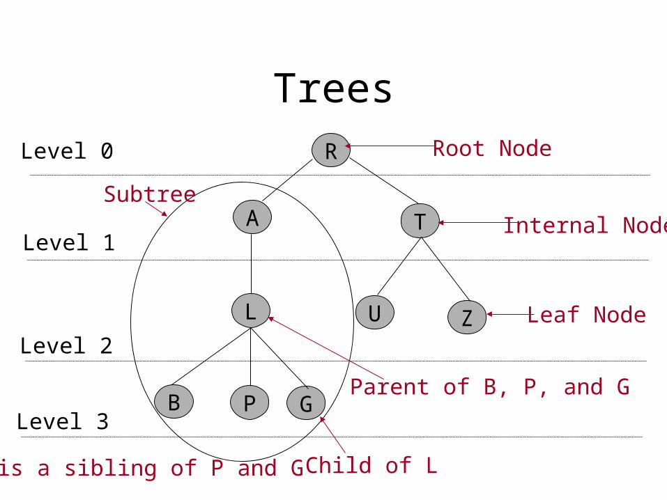
TreesR

A T

L U

GPB

Z

Level 0

Level 1

Level 2

Level 3

Root Node

Internal Node

Leaf Node

Subtree

Child of L

Parent of B, P, and G

B is a sibling of P and G

Tree Facts

• Each node (except the root node) has exactly one parent node.

• Once a link is followed from a parent to a child, it is not possible to get to the parent by following more links. – There are not cycles in trees.

• The children of a node are trees themselves. (subtrees)

Binary Tree

• A binary tree has a finite set of nodes that are either empty or consist of exactly one root node and at most two disjoint binary trees (left and right).– Each node may have at most two children.

Binary Search Tree

• A binary Search Tree contains all nodes with a value less than the parent in the left subtree, and all values greater than the parent in the right subtree.

Binary Search Trees

K

G

D

A

Q

M T

O

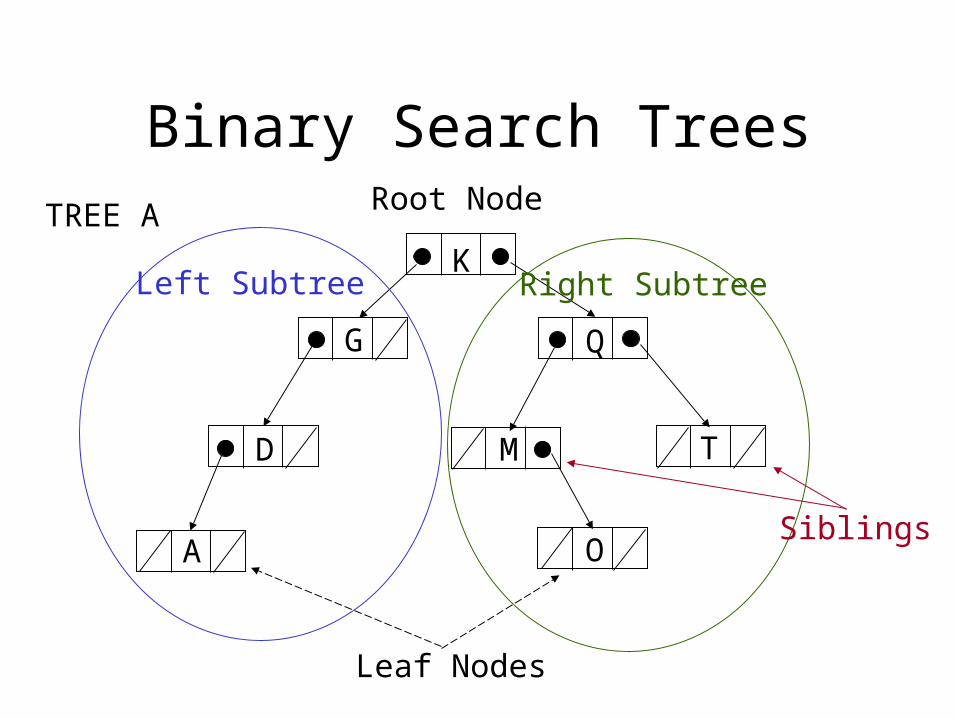
Left Subtree Right Subtree

Root Node

Leaf Nodes

Siblings

TREE A

Binary Search Trees

• New nodes may only be added to leaf nodes.

• A tightly packed tree is one in which the number of nodes at each level contains about twice as many as the previous level.

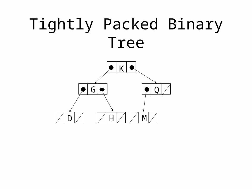
Tightly Packed Binary Tree

K

G

D

Q

MH

Traversing Trees

• Traversing a tree is the order in which the elements of the tree are visited.– Each element may be visited only once.

Breadth First Traversal

• A Breadth First Traversal visits all the nodes at a particular level from left to right and then moves to the next level.– The traversal ends when the right most

node of the last level has been visited.– The traversal begins at the root node.– The output for TREE A would be: K, G, Q,

D, M, T, A, O

Depth First Traversals

• A Depth First Traversal visits nodes throughout the levels until it reaches the bottom and then starts over with another subtree.– There are a total of 8 depth first traversal methods.– We will talk about three:

• In-order

• Pre-order

• Post-order

In-order Traversal

• An In-order Traversal visits the nodes in ascending order.– First you visit the left subtree, then the root

(or parent node), and then the right subtree (recursively).

• The output for TREE A would be: A, D, J, K, M, O, Q, T

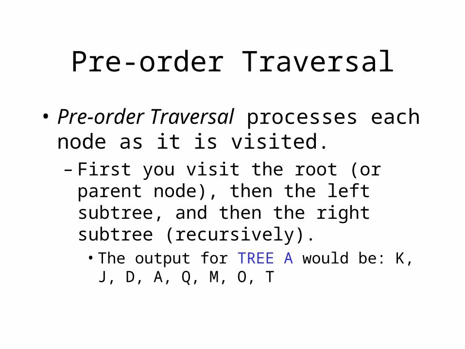
Pre-order Traversal

• Pre-order Traversal processes each node as it is visited.– First you visit the root (or parent node),

then the left subtree, and then the right subtree (recursively).

• The output for TREE A would be: K, J, D, A, Q, M, O, T

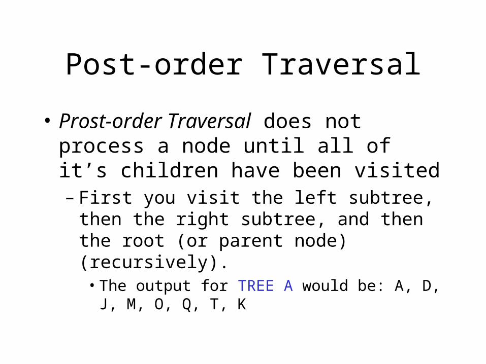
Post-order Traversal

• Prost-order Traversal does not process a node until all of it’s children have been visited– First you visit the left subtree, then the right

subtree, and then the root (or parent node) (recursively).

• The output for TREE A would be: A, D, J, M, O, Q, T, K

Binary Trees

• A full binary tree is a binary tree where every leaf has the same depth, and every non-leaf has two children.

K

G

D

Q

M TI

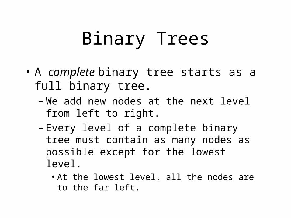
Binary Trees

• A complete binary tree starts as a full binary tree.– We add new nodes at the next level from

left to right.– Every level of a complete binary tree must

contain as many nodes as possible except for the lowest level.

• At the lowest level, all the nodes are to the far left.

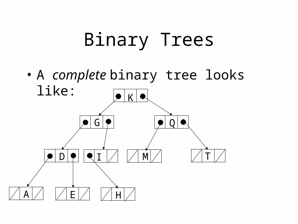
Binary Trees

• A complete binary tree looks like:

K

G

D

Q

M TI

A E H

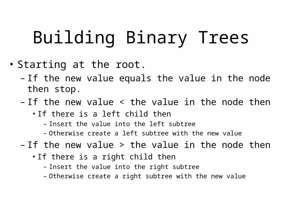
Building Binary Trees

• Starting at the root.– If the new value equals the value in the node then stop.– If the new value < the value in the node then

• If there is a left child then– Insert the value into the left subtree– Otherwise create a left subtree with the new value

– If the new value > the value in the node then• If there is a right child then

– Insert the value into the right subtree– Otherwise create a right subtree with the new value

Example

• Build a binary search trees for the following:– 7, 4, 2, 6, 1, 3, 5, 7– 7, 1, 2, 3, 4, 5, 6, 7– 8, 7, 6, 5, 4, 3, 2, 1– 7, 4, 2, 1, 7, 3, 6, 5

Searching a Binary Tree• Begin at the root• Until the value is found OR there are no more

nodes– If the value in the node matches the search key then

• Stop, we are done.• Otherwise,

– If the value is less, then » Look in the left subtree» Otherwise, look in the right subtree

• Requires log2N for balanced trees.

Creating Trees

• A Binary tree can be easily represented as an array.

• Usually, we actually implement a tree using a Node class.– Node.java– BinarySearchTree.java

Creating a Coding Tree

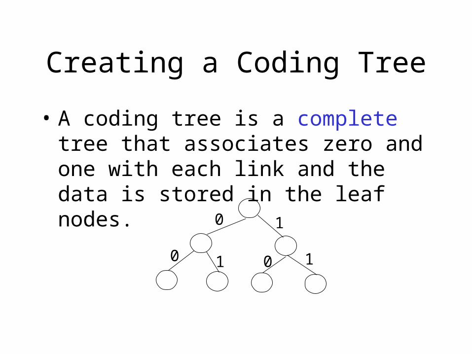
• A coding tree is a complete tree that associates zero and one with each link and the data is stored in the leaf nodes.

0

0 0

1

1 1

Coding Tree Example• Assume we have the following information for

the string “Go Go Gophers”, create a coding tree.

• G – 10• O – 11• P – 0100• H – 0101• E – 0110• R – 0111• S – 000• ‘ ‘ - 001

Coding Trees

• Using the 0/1 convention for the coding tree is called the prefix property.– This means that no bit-sequence of a

character is the prefix of any other bit-sequence encoding.

Huffman Coding

• Huffman Coding is widely used to effectively compress data. – As opposed to using ASCII or UNICODE.– Every piece of data entered into the computer

is converted to a binary representation.• With ASCII this representation requires 8 bits per

character.• With Huffman Coding we can save between 20%

to 90% of the bits.

Huffman Coding

• The idea behind Huffman Coding is to represent the most frequently used characters with fewer bits.– Each character has a weight associated with it

which is the frequency that the character appears in the string to encode.

– Each individual character is considered to be a tree and to have an associated weight.

Huffman Coding

– Then the trees are combined by choosing the two trees with the smallest weight and creating a new tree.

• This continues until all the trees are combined into one tree.

– The result should be a fewer number of bits for the most frequently used characters.

– Huffman Coding example handout.