data warehousing & data mining - tu · pdf filedata warehousing & data mining...

Data Warehousing & Data Mining& Data MiningWolf-Tilo BalkeSilviu HomoceanuInstitut für InformationssystemeTechnische Universität Braunschweighttp://www.ifis.cs.tu-bs.de

9. Business Intelligence

9.1 Business Intelligence Overview

9.2 Principles of Data Mining

9.3 Association Rule Mining

9. Business Intelligence

DW & DM – Wolf-Tilo Balke – Institut für Informationssysteme – TU Braunschweig 2

• What is Business Intelligence (BI)?

– The process, technologies and tools needed to turn data into information, information into knowledge and knowledge into plans that drive profitable business action

9.1 BI Overview

business action

– BI comprises data warehousing, business analytic tools, and content/knowledge management


• Typical BI applications are

– Customer segmentation

– Propensity to buy (customer disposition to buy)

– Customer profitability

9.1 BI Overview

Customer profitability

– Fraud detection

– Customer attrition (loss of customers)

– Channel optimization (connecting with the customer)


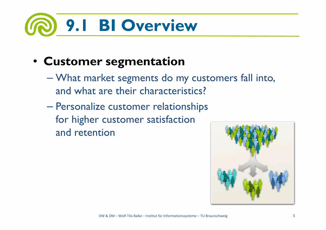
• Customer segmentation

– What market segments do my customers fall into, and what are their characteristics?

– Personalize customer relationshipsfor higher customer satisfaction

9.1 BI Overview

for higher customer satisfaction and retention


• Propensity to buy

– Which customers are most likely to respond to mypromotion?

– Target customers based on their need to increase their loyalty to your product line

9.1 BI Overview

their loyalty to your product line

• Also, increase campaign profitability by focusing on the customers most likely to buy


• Customer profitability

– What is the lifetime profitability of my customer?

– Make individual business interaction decision based on the overall profitability of customers

9.1 BI Overview


• Fraud detection

– How can I tell which transactions are likely to be fraudulent?

• If your wife has just proposed to increase your life insurance policy,

9.1 BI Overview

increase your life insurance policy, you should probably order pizza for a while

– Quickly determine fraud and take immediate action to minimize damage


• Customer attrition

– Which customer is at risk of leaving?

– Prevent loss of high-value customersand let go of lower-value customers

9.1 BI Overview

• Channel optimization

– What is the best channel to reach my customer in each segment?

– Interact with customers based on their preference and your need to manage cost


• BI architecture

9.1 BI Overview


• Automated decision tools

– Rule-based systems that provide a solution usually in one functional area to a specific repetitive management problem in one industry

• E.g., automated loan approval, intelligent price setting

9.1 BI Overview

• E.g., automated loan approval, intelligent price setting

• Business performance management (BPM)

– Based on the balanced scorecard methodology

– A framework for defining, implementing, and managing an enterprise’s business strategy by linking objectives with factual measures


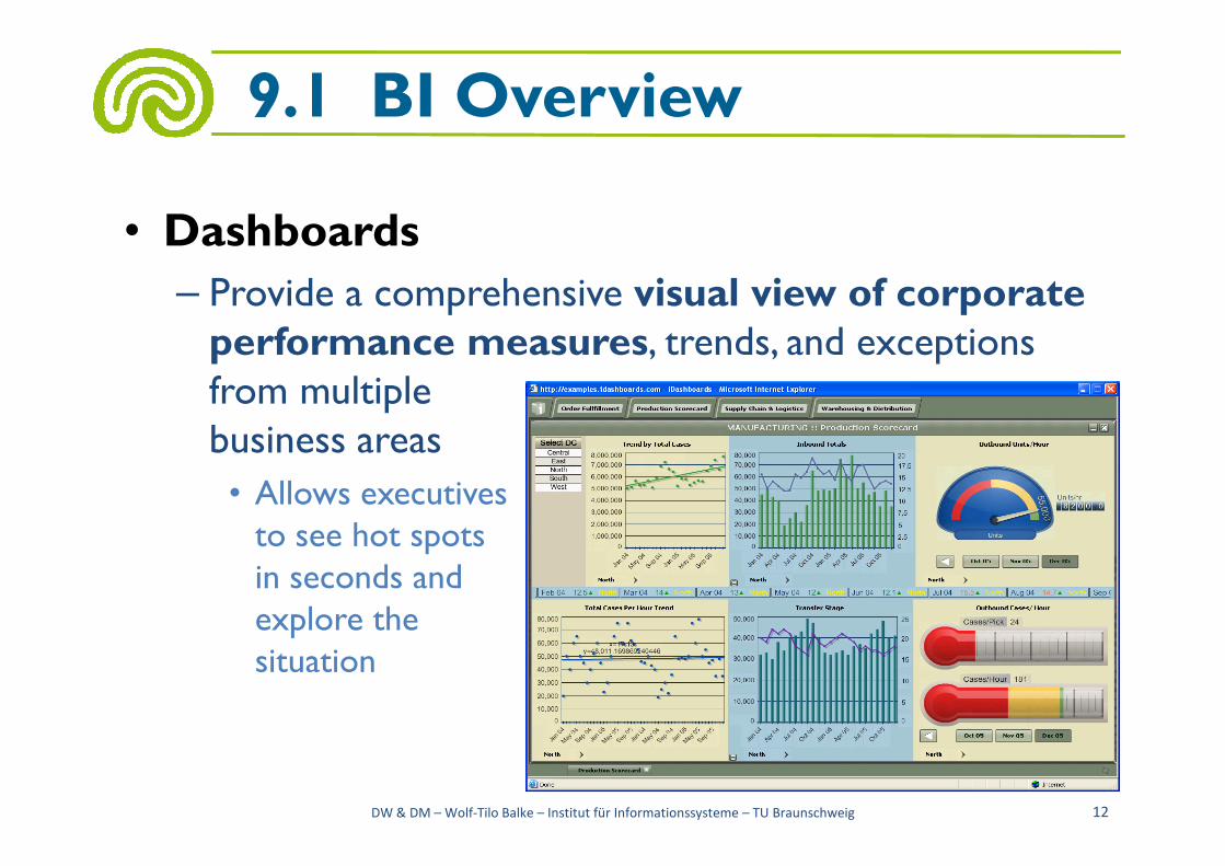
• Dashboards

– Provide a comprehensive visual view of corporate performance measures, trends, and exceptions from multiplebusiness areas

9.1 BI Overview

business areas

• Allows executivesto see hot spots in seconds andexplore thesituation


• What is data mining(knowledge discovery indatabases)?

– Extraction of interesting(non-trivial, implicit,

9.2 Data Mining

(non-trivial, implicit,previously unknown and potentially useful) information or patterns from data in large databases

• What is not data mining?

– (Deductive) query processing

– Expert systems or small ML/statistical programs


• Data Mining applications– Database analysis and decision

support• Market analysis and management

• Risk analysis and management e.g., forecasting, customer

9.2 Principles of DM

• Risk analysis and management e.g., forecasting, customer retention, improved underwriting, quality control, competitive analysis

• Fraud detection and management

– Other Applications• Text mining (news group, email, documents) and Web

analysis (Google Analytics)

• Intelligent query answering


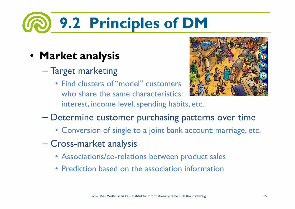
• Market analysis

– Target marketing

• Find clusters of “model” customerswho share the same characteristics:interest, income level, spending habits, etc.


interest, income level, spending habits, etc.

– Determine customer purchasing patterns over time

• Conversion of single to a joint bank account: marriage, etc.

– Cross-market analysis

• Associations/co-relations between product sales

• Prediction based on the association information


– Customer profiling

• Data mining can tell you what types of customers buy what products (clustering or classification)

– Identifying customer requirements

• Identifying the best products for different customers


• Identifying the best products for different customers

• Use prediction to find what factors will attract new customers

– Provide summary information

• Various multidimensional summary reports

• Statistical summary information (data central tendency and variation)


• Corporate analysis and risk management– Finance planning and asset evaluation

• Cash flow analysis and prediction• Contingent claim analysis to evaluate

assets • Cross-sectional and time series analysis

(financial-ratio, trend analysis, etc.)


• Cross-sectional and time series analysis(financial-ratio, trend analysis, etc.)

– Resource planning• Summarize and compare the resources

and spending

– Competition• Monitor competitors and market directions • Group customers into classes and a class-based pricing

procedure• Set pricing strategy in a highly competitive market


• Fraud detection and management– Applications

• Widely used in health care, retail, credit card services, telecommunications (phone card fraud), etc.

– Approach


– Approach• Use historical data to build models of fraudulent behavior

and use data mining to help identify similar instances

– Examples• Car insurance: detect a group of people who stage

accidents to collect claims

• Money laundering: detect suspicious money transactions (US Treasury's Financial Crimes Enforcement Network)


• Other applications– Sports

• IBM Advanced Scout analyzed NBA game statistics (shots blocked, assists, and fouls) to gain competitive advantage for New York Knicks and Miami Heat

– Astronomy


– Astronomy• JPL and the Palomar Observatory discovered 22 quasars with the

help of data mining

– Internet Web Surf-Aid• IBM Surf-Aid applies data mining algorithms to Web access logs

for market-related pages to discover customer preference and behavior pages, analyzing effectiveness of Web marketing, improving Web site organization, etc.


• Architecture of DM systems


Pattern evaluation

Graphical user interface


Data

Warehouse

ETL Filtering

Database or data warehouse server

Data mining engine

Knowledge-base

Databases

• DM functionalities

– Association (correlation and causality)

• Multi-dimensional vs. single-dimensional association

• age(X, “20..29”) , income(X, “20..29K”) ⟶ buys(X, “PC”) [support = 2%, confidence = 60%]

⟶


⟶

[support = 2%, confidence = 60%]

• contains(T, “computer”) ⟶ contains(x, “software”) [1%, 75%]

– Classification and Prediction

• Finding models (functions) that describe and distinguish classes or concepts for future predictions, e.g., classify countries based on climate, or classify cars based on gas mileage

• Presentation: decision-tree, classification rule, neural network

• Prediction: predict some unknown or missing numerical values


– Cluster analysis

• Class label is unknown: group data to form new classes, e.g., cluster houses to find distribution patterns

• Clustering based on the principle: maximizing the intra-class similarity and minimizing the interclass similarity


similarity and minimizing the interclass similarity

– Outlier analysis

• Outlier: a data object that does not comply with the general behavior of the data

• Can be considered as noise or exception, but is quite useful in fraud detection, rare events analysis


– Trend and evolution analysis

• Trends and deviation can be detected by regression analysis

• Sequential pattern mining, periodicity analysis

• Similarity-based analysis



• Association rule mining has the objective of finding all co-occurrence relationships (called associations), among data items

– Classical application: market basket data analysis, which aims to discover how items are purchased by


which aims to discover how items are purchased by customers in a supermarket

• E.g., Cheese ⟶ Wine [support = 10%, confidence = 80%]meaning that 10% of the customers buy cheese and wine together, and 80% of customers buying cheese also buy wine


• Basic concepts of association rules

– Let I = {i1, i2, …, im} be a set of items.Let T = {t1, t2, …, tn} be a set oftransactions where each transaction ti isa set of items such that ti ⊆ I.


T = {t , t , …, t }

ti

a set of items such that ti ⊆ I.

– An association rule is an implication of the form:X ⟶ Y, where X ⊂ I, Y ⊂ I and X ⋂ Y = ∅


• Association rule mining marketbasket analysis example – I – set of all items sold in a store

• E.g., i1 = Beef, i2 = Chicken, i3 = Cheese, …

– T – set of transactions

t t t


i1 i2 i3

– T – set of transactions• The content of a customers basket

• E.g., t1: Beef, Chicken, Milk; t2: Beef, Cheese; t3: Cheese, Boots; t4: …

– An association rule might be• Beef, Chicken ⟶ Milk, where {Beef, Chicken} is X and

{Milk} is Y


• Rules can be weak or strong

– The strength of a rule is measured by itssupport and confidence

– The support of a rule X ⟶ Y, is the percentage of transactions in T that contains X and Y

Pr({X,Y} ⊆ t )


X ⟶ Y

transactions in T that contains X and Y

• Can be seen as an estimate of the probability Pr({X,Y} ⊆ ti)

• With n as number of transactions in T the support of the rule X ⟶ Y is:

supportsupportsupportsupport = |{i | {X, Y} ⊆ ti}| / n


– The confidence of a rule X ⟶ Y, is the percentage of transactions in T containing X, that contain X ∪ Y

• Can be seen as estimate of the probability Pr(Y ⊆ ti |X ⊆ ti)

confidenceconfidenceconfidenceconfidence = |{i | {X, Y} ⊆ ti}| / |{j | X ⊆ tj}|


confidenceconfidenceconfidenceconfidence = |{i | {X, Y} ⊆ ti}| / |{j | X ⊆ tj}|


• How do we interpret support and confidence?– If support is too low, the rule may just occur due to

chance• Acting on a rule with low support may not be profitable

since it covers too few cases

YX


since it covers too few cases

– If confidence is too low, we cannot reliably predict Yfrom X

• Objective of mining association rules is to discover all associated rules in T that have support and confidence greater than a minimum threshold (minsup, minconf)!


• Finding rules based on support and confidence thresholds

– Let minsup = 30% andminconf = 80%

– Chicken, Clothes ⟶ Milk


Transactions

T1 Beef, Chicken, Milk

T2 Beef, Cheese

T3 Cheese, Boots

– Chicken, Clothes ⟶ Milk is valid, [sup = 3/7(42.84%), conf = 3/3(100%)]

– Clothes ⟶ Milk, Chicken is also valid, and there are more…


T3 Cheese, Boots

T4 Beef, Chicken, Cheese

T5 Beef, Chicken, Clothes, Cheese, Milk

T6 Clothes, Chicken, Milk

T7 Chicken, Milk, Clothes

• This is rather a simplistic view of shopping baskets – Some important information is not considered, e.g.,

the quantity of each item purchased, the price paid,…

• There are a large number of rule mining


• There are a large number of rule mining algorithms– They use different strategies and data structures

– Their resulting sets of rules are all the same• Given a transaction data set T, and a minimum support and a

minimum confident, the set of association rules existing in T is uniquely determined


• Approaches in association rule mining

– Apriori algorithm

– Mining with multiple minimum supports

– Mining class association rules



• The best known mining algorithm is the Apriorialgorithm– Definition

• Frequent itemset is an itemset whose support is ≥ minsup

– Two steps:

9.3 AprioriAlgorithm

– Two steps:• Find all frequent itemsets (also called large itemsets)

• Use frequent itemsets to generate rules

• E.g., a frequent itemset– {Chicken, Clothes, Milk} [sup = 3/7]

• And one rule from the frequent itemset– Clothes ⟶ Milk, Chicken [sup = 3/7, conf = 3/3]


• Step 1: frequent itemset generation

– Key idea:

• The apriori property (downward closure property): Any subset of a frequent itemset is also a frequent itemset

• E.g., for minsup = 30%

9.3 Apriori Algorithm: Step 1

• E.g., for minsup = 30%


Transactions

T1 Beef, Chicken, Milk

T2 Beef, Cheese

T3 Cheese, Boots

T4 Beef, Chicken, Cheese

T5 Beef, Chicken, Clothes, Cheese, Milk

T6 Clothes, Chicken, Milk

T7 Chicken, Milk, Clothes

Chicken, Clothes, Milk

Chicken, Clothes Chicken, Milk Clothes, Milk

Chicken Clothes Milk

• Finding frequent items

– Idea:

• Find all 1-item frequent itemsets; then all 2-item frequent itemsets, etc.

• In each iteration k, only consider itemsets that contain an


• In each iteration k, only consider itemsets that contain ank-1 frequent itemset

• Optimization: the algorithm assumes that items are sorted in lexicographic order

– The order is used throughout the algorithm in each itemset

– {w[1], w[2], …, w[k]} represents a k-itemset w consisting of items w[1], w[2], …, w[k], where w[1] < w[2] < … < w[k] according to the lexicographic order


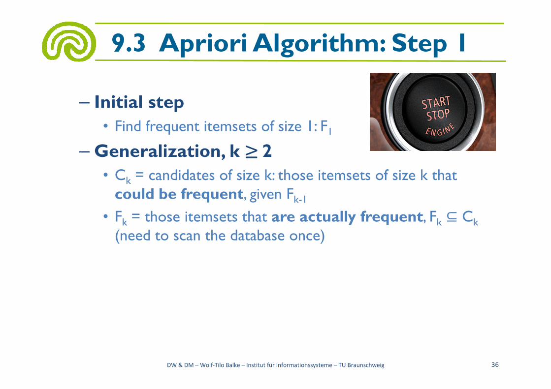
– Initial step

• Find frequent itemsets of size 1: F1

– Generalization, k ≥ ≥ ≥ ≥ 2

• Ck = candidates of size k: those itemsets of size k that could be frequent, given Fk-1

⊆


≥ ≥ ≥ ≥

could be frequent, given Fk-1

• Fk = those itemsets that are actually frequent, Fk ⊆ Ck

(need to scan the database once)


– Generalization of candidates uses Fk-1 as input and returns a superset (candidates) of the set of all frequent k-itemsets. It has two steps:

• Join step: generate all possible candidate itemsets Ck of length k, e.g., Ik = join(Ak-1, Bk-1) ⟺ Ak-1= {i1, i2, …, ik-2, ik-1}


length k, e.g., Ik = join(Ak-1, Bk-1) ⟺ Ak-1= {i1, i2, …, ik-2, ik-1} and Bk-1= {i1, i2, …, ik-2, i’k-1} and ik-1< i’k-1; Then Ik = {i1, i2, …, ik-2, ik-1, i’k-1}

• Prune step: remove those candidates in Ck that do not respect the downward closure property (include k-1 non-frequent subsets)


– Generalization e.g., F3 = {{1, 2, 3}, {1, 2, 4}, {1, 3, 4}, {1, 3, 5}, {2, 3, 4}}

• Join


{1, 2, 4} {1, 3, 4}

{1, 3, 5}

{1, 2, 3} {1, 2, 4}

{1, 3, 4}

{1, 2, 3, 4}


{2, 3, 4}

{1, 3, 5}

{1, 3, 5} {2, 3, 4}

{2, 3, 4}

{1, 3, 4}

{1, 3, 5}

{1, 3, 4}

{2, 3, 4}

{1, 3, 5} {1, 3, 4, 5}

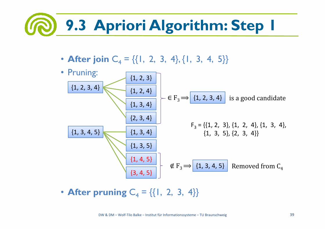
• After join C4 = {{1, 2, 3, 4}, {1, 3, 4, 5}}

• Pruning:


{1, 2, 3, 4}

{2, 3, 4}

{1, 2, 3}

{1, 2, 4}

{1, 3, 4}{1, 2, 3, 4}∈ F3 ⟹ is a good candidate

• After pruning C4 = {{1, 2, 3, 4}}


{2, 3, 4}F3 = {{1, 2, 3}, {1, 2, 4}, {1, 3, 4},

{1, 3, 5}, {2, 3, 4}}{1, 3, 4, 5}

{3, 4, 5}

{1, 3, 4}

{1, 3, 5}

{1, 4, 5}{1, 3, 4, 5}∉ F3 ⟹ Removed from C4

• Finding frequent items, example,minsup = 0.5

– First T scan ({item}:count)

• C1: {1}:2, {2}:3, {3}:3, {4}:1, {5}:3

• F : {1}:2, {2}:3, {3}:3, {5}:3;


TID Items

T100 1, 3, 4

T200 2, 3, 5

T300 1, 2, 3, 5

T400 2, 5

• F1: {1}:2, {2}:3, {3}:3, {5}:3; {4} has a support of ¼ < 0.5 so it does not belong to the

frequent items

• C2 = prune(join(F1)) join : {1,2}, {1,3}, {1,5}, {2,3}, {2,5}, {3,5};prune: C2 : {1,2}, {1,3}, {1,5}, {2,3}, {2,5}, {3,5}; (all items belong to F1)


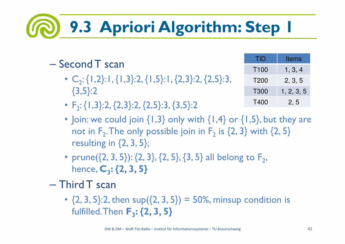
– Second T scan

• C2: {1,2}:1, {1,3}:2, {1,5}:1, {2,3}:2, {2,5}:3,{3,5}:2

• F2: {1,3}:2, {2,3}:2, {2,5}:3, {3,5}:2

• Join: we could join {1,3} only with {1,4} or {1,5}, but they are


TID Items

T100 1, 3, 4

T200 2, 3, 5

T300 1, 2, 3, 5

T400 2, 5

• Join: we could join {1,3} only with {1,4} or {1,5}, but they are not in F2. The only possible join in F2 is {2, 3} with {2, 5} resulting in {2, 3, 5};

• prune({2, 3, 5}): {2, 3}, {2, 5}, {3, 5} all belong to F2, hence, C3: {2, 3, 5}

– Third T scan

• {2, 3, 5}:2, then sup({2, 3, 5}) = 50%, minsup condition is fulfilled. Then F3: {2, 3, 5}


• Step 2: generating rules from frequent itemsets

– Frequent itemsets are not the same as association rules

– One more step is needed to generate association rules: for each frequent itemset I, for each proper

X I


rules: for each frequent itemset I, for each proper nonempty subset X of I:

• Let Y = I \ X; X ⟶ Y is an association rule if:

– Confidence(X ⟶ Y) ≥ minconf,

– Support(X ⟶ Y) := |{i | {X, Y} ⊆ ti}| / n = support(I)

– Confidence(X ⟶ Y) := |{i | {X, Y} ⊆ ti}| / |{j | X ⊆ tj}|

= support(I) / support(X)


• Rule generation example, minconf = 50%– Suppose {2, 3, 5} is a frequent itemset, with sup=50%, as

calculated in step 1– Proper nonempty subsets: {2, 3}, {2, 5}, {3, 5}, {2}, {3}, {5},

with sup=50%, 75%, 50%, 75%, 75%, 75% respectively– These generate the following association rules:

2,3 ⟶ 5, confidence=100%; (sup(I)=50%; sup{2,3}=50%; 50/50= 1)


– These generate the following association rules:• 2,3 ⟶ 5, confidence=100%; (sup(I)=50%; sup{2,3}=50%;

50/50= 1)

• 2,5 ⟶ 3, confidence=67%; (50/75)

• 3,5 ⟶ 2, confidence=100%; (…)

• 2 ⟶ 3,5, confidence=67%



– All rules have support = support(I) = 50%


TID Items

T100 1, 3, 4

T200 2, 3, 5

T300 1, 2, 3, 5

T400 2, 5

• Rule generation, summary

– In order to obtain X ⟶ Y, we need toknow support(I) and support(X)

– All the required information for confidence computation has already been recorded in itemset


I X

computation has already been recorded in itemsetgeneration

• No need to read the transactions data any more

• This step is not as time-consuming as frequent itemsetsgeneration


• Apriori Algorithm, summary

– If k is the size of the largest itemset, then it makes at most k passes over data (in practice, k is bounded e.g., 10)

– The algorithm is very fast: under some conditions, all rules can be found in linear time

9.3 AprioriAlgorithm

can be found in linear time

– Scales up to large data sets

– The mining exploits sparseness of data, and high minsupand minconf thresholds

– High minsup threshold makes it impossible to find rules involving rare items in the data. The solution is a mining with multiple minimum supports approach


• Mining with multiple minimum supports

– Single minimum support assumes that all items in the data are of the same nature and/or have similar frequencies, which is incorrect…

– In practice, some items appear very frequently in the

9.3 Multiple Minimum Supports

– In practice, some items appear very frequently in the data, while others rarely appear

• E.g., in a supermarket, people buy cooking pans much less frequently than they buy bread and milk


• Rare item problem: if the frequencies of items vary significantly, we encounter two problems

– If minsup is set too high, those rules that involve rare items will not be found

– To find rules that involve both frequent and rare items,


– To find rules that involve both frequent and rare items, minsup has to be set very low. This may cause combinatorial explosion because those frequent items will be associated with one another in all possible ways


• Multiple Minimum Supports

– Each item can have a minimum item support

• Different support requirements for different rules

– To prevent very frequent items and very rare items from appearing in the same itemset S, we introduce a

φ


from appearing in the same itemset S, we introduce a support difference constraint (φ)

• maxi∈S{sup(i)} - mini∈S {sup(i)} ≤ φ,

where 0 ≤ φ ≤ 1 is user specified


• Minsup of a rule

– Let MIS(i) be the minimum item support (MIS) value of item i. The minsup of a rule R is the lowest MIS value of the items in the rule:

• Rule R: i1, i2, …, ik ⟶ ik+1, …, ir satisfies its minimum support ≥ min(MIS(i ), MIS(i ), …, MIS(i ))


• Rule R: i1, i2, …, ik ⟶ ik+1, …, ir satisfies its minimum support if its actual support is ≥ min(MIS(i1), MIS(i2), …, MIS(ir))

• E.g., the user-specified MIS values are as follows:MIS(bread) = 2%, MIS(shoes) = 0.1%, MIS(clothes) = 0.2%

– clothes ⟶ bread [sup=0.15%,conf =70%] doesn’t satisfy its minsup

– clothes ⟶ shoes [sup=0.15%,conf =70%] satisfies its minsup


• Downward closure property isnot valid anymore

– E.g., consider four items 1, 2, 3and 4 in a databaseTheir minimum item supports are


Their minimum item supports are

• MIS(1) = 10%, MIS(2) = 20%, MIS(3) = 5%, MIS(4) = 6%

• {1, 2} with a support of 9% is infrequent since min(10%, 20%) > 9%, but {1, 2, 3} could be frequent, if it would have a support of e.g. , 7%

– If applied, downward closure, eliminates {1, 2} so that {1, 2, 3} is never evaluated


• How do we solve the downward closure property problem?

– Sort all items in I according to their MIS values (make it a total order)

• The order is used throughout the algorithm in each itemset


I

• The order is used throughout the algorithm in each itemset

– Each itemset w is of the following form:

• {w[1], w[2], …, w[k]}, consisting of items, w[1], w[2], …, w[k], where MIS(w[1]) ≤ MIS(w[2]) ≤ … ≤ MIS(w[k])


• Multiple minimum supports is an extension of the Apriori algorithm

– Step 1: frequent itemset generation

• Initial step

– Produce the seeds for generating candidate itemsets


– Produce the seeds for generating candidate itemsets

• Candidate generation

– For k = 2

• Generalization

– For k > 2, pruning step differs from the Apriori algorithm

– Step 2: rule generation


• Step 1: frequent itemset generation

– Initial step

• Sort I according to the MIS value of eachitem. Let M represent the sorted items

• Scan the data once to record the support

9.3 Multiple Minimum Supports: Step 1

• Scan the data once to record the supportcount of each item

• Go through the items in M to find the first item i, that meets MIS(i). Insert it into a list of seeds L

• For each subsequent item j in M (after i), if sup(j) ≥ MIS(i), then insert j in L

• Calculate F1 from L based on MIS of each item in L


– E.g., I={1, 2, 3, 4}, with given MIS(1)=10%, MIS(2)=20%, MIS(3)=5%, MIS(4)=6%, and consider n=100 transactions:

• Sort I, in M = {3, 4, 1, 2}

• Record support count ({item}:count) e.g., {3}:6, {4}:3, {1}:9


I M

• Record support count ({item}:count) e.g., {3}:6, {4}:3, {1}:9 and {2}:25

• MIS(3) = 5%; sup ({3}) = 6%; sup(3) > MIS(3), so L={3}Sup({4}) = 3% < MIS(3), so L remains {3}Sup({1}) = 9% > MIS(3), L = {3, 1}Sup({2}) = 25% > MIS(3), L = {3, 1, 2}

• F1 = {{3}, {2}}, since sup({1}) = 9% < MIS(1)


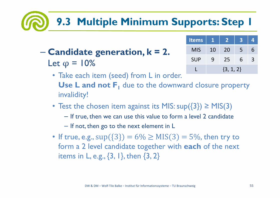
– Candidate generation, k = 2.Let φ = 10%

• Take each item (seed) from L in order.Use L and not F1 due to the downward closure property invalidity!


Items 1 2 3 4

MIS 10 20 5 6

SUP 9 25 6 3

L {3, 1, 2}

invalidity!

• Test the chosen item against its MIS: sup({3}) ≥ MIS(3)

– If true, then we can use this value to form a level 2 candidate

– If not, then go to the next element in L

• If true, e.g., sup({3}) = 6% ≥ MIS(3) = 5%, then try to form a 2 level candidate together with each of the next items in L, e.g., {3, 1}, then {3, 2}


– {3, 1} is a candidate :⟺ sup({1})≥ MIS(3) and|sup({3}) – sup({1})| ≤ φ

• sup({1}) = 9%; MIS(3) = 5%; sup({3}) = 6%; φ := 10%9% > 5% and |6%-9%| < 10%, thus C2 = {3, 1}

– Now try {3, 2}


– Now try {3, 2}

• sup({2}) = 25%; 25% > 5% but |6%-25%| > 10% so this candidate will be rejected due to the support difference constraint


Items 1 2 3 4

MIS 10 20 5 6

SUP 9 25 6 3

L {3, 1, 2}

– Pick the next seed from L, i.e. 1 (needed to try {1,2})

• sup({1}) < MIS(1) so we can not use1 as seed!

– Candidate generation for k=2 remains C2 = {3, 1}


Items 1 2 3 4

MIS 10 20 5 6

SUP 9 25 6 3

L {3, 1, 2}

– Candidate generation for k=2 remains C2 = {3, 1}

• Now read the transaction list and calculate the support of each item in C2. Let’s assume sup({3, 1})=6, which is larger than min(MIS(3), MIS(1))

• Thus F2 = {3, 1}


– Generalization, k > 2 uses Fk-1 as input and returns a superset (candidates) of the set of all frequent k-itemsets. It has two steps:

• Join step: same as in the case of k=2Ik = join(Ak-1, Bk-1) ⟺ Ak-1= {i1, i2, …, ik-2, ik-1} and Bk-1= {i1, i2,

≤≤≤≤φφφφ.


Ik = join(Ak-1, Bk-1) ⟺ Ak-1= {i1, i2, …, ik-2, ik-1} and Bk-1= {i1, i2, …, ik-2, i’k-1} and ik-1< i’k-1 and |sup(ik-1) – sup(i’k-1)| ≤≤≤≤φφφφ.

Then Ik = {i1, i2, …, ik-2, ik-1, i’k-1}

• Prune step: for each (k-1) subset s of Ik, if s is not in Fk-1, then Ik can be removed from Ck (it is not a good candidate). There is however one exception to this rule, when s does not include the first item from Ik


– Generalization, k > 2 example: let’s considerF3={{1, 2, 3}, {1, 2, 5}, {1, 3, 4}, {1, 3, 5}, {1, 4, 5}, {1, 4, 6}, {2, 3, 5}}

• After join we obtain {1, 2, 3, 5}, {1, 3, 4, 5} and {1, 4, 5, 6} (we do not consider the support difference constraint)


do not consider the support difference constraint)

• After pruning we get C4 = {{1, 2, 3, 5}, {1, 3, 4, 5}}

– {1, 2, 3, 5} is ok

– {1, 3, 4, 5} is not deleted although {3, 4, 5} ∉ F3, because MIS(3) > MIS(1). If MIS(3) = MIS(1), it could be deleted

– {1, 4, 5, 6} is deleted because {1, 5, 6} ∉ F3


• Step 2: rule generation– Downward closure property is not valid anymore,

therefore we have frequent k order items, which contain (k-1) non-frequent sub-items

• In the Apriori algorithm we only recorded the support of frequent itemsets


frequent itemsets

• For those non-frequent items we do not have the support value recorded

• This problem arises when we form rules of the formA,B ⟶ C, where MIS(C) = min(MIS(A), MIS(B), MIS(C)). It is called head-item problem

– Besides the head-item problem, the rule generation works exactly as in the Apriori algorithm


• Rule generationexample

– {Shoes, Clothes, Bread} is a frequent itemset since

• MIS({Shoes, Clothes, Bread}) = 0.1 < sup({Shoes, Clothes, Bread}) = 0.12


Items Bread Clothes Shoes

MIS 2 0.2 0.1

Items {Clothes, Bread} {Shoes, Clothes, Bread}

SUP 0.15 0.12

Bread}) = 0.12

– However {Clothes, Bread} is not (since 0.2 > 0.15)

• So we may not calculate the confidence of all rules depending on Shoes, i.e. rules:

– Clothes, Bread ⟶ Shoes

– Clothes ⟶ Shoes, Bread

– Bread ⟶ Shoes, Clothes


– Head-item problem, e.g., Clothes, Bread ⟶ Shoes; Clothes ⟶ Shoes, Bread; Bread ⟶ Shoes, Clothes

• If we have some item on the right side of a rule, which has the minimum MIS (e.g., Shoes), we may not be able to calculate the confidence without reading the data again


calculate the confidence without reading the data again

• Solution is to record also the support of only one non-frequent sub-itemset, the itemset obtained by eliminating the item with the minimum MIS e.g.,

– {Clothes, Bread, Shoes} – {Shoes} = {Clothes, Bread}


• Advantages

– It is a more realistic model for practical applications

– The model enables us to find rare item rules, but without producing a huge number of meaningless rules with frequent items


rules with frequent items

– By setting MIS values of some items to 100% (or more), we can effectively instruct the algorithms not to generate rules only involving these items


• Mining Class Association Rules (CAR)

– Normal association rule mining does nothave any target

• It finds all possible rules that exist in data, i.e., any item can appear as a consequent or a condition of a rule


appear as a consequent or a condition of a rule

– However, in some applications, the user is interested in some targets

• E.g., the user has a set of text documents from some known topics. He wants to find out what words are associated or correlated with each topic


• CAR, example– A text document data set

• doc 1: Student, Teach, School : Education

• doc 2: Student, School : Education

• doc 3: Teach, School, City, Game : Education

• doc 4: Baseball, Basketball : Sport

9.3 Class Association Rules

• doc 4: Baseball, Basketball : Sport

• doc 5: Basketball, Player, Spectator : Sport

• doc 6: Baseball, Coach, Game, Team : Sport

• doc 7: Basketball, Team, City, Game : Sport

– Let minsup = 20% and minconf = 60%. Examples of class association rules:

• Student, School ⟶ Education [sup= 2/7, conf = 2/2]

• Game ⟶ Sport [sup= 2/7, conf = 2/3]


• CAR algorithm– Unlike normal association rules, CARs can be mined

directly in one step

– The key operation is to find all rule-items that have support above minsup

⊆ ∈


support above minsup• A rule-item is of the form (condset, y), where condset is a

set of items from I (i.e., condset ⊆ I), and y ∈ Y is a class label where I ⋂ Y = ∅

– Each rule-item basically represents a rule• condset ⟶ y

– The Apriori algorithm can be modified to generate CARs


• CAR can also be extended with multiple minimum supports

– The user can specify different minimum supports to different classes, which effectively assign a different minimum support to rules of each class


minimum support to rules of each class

• E.g., a data set with two classes, Yes and No. We may want rules of class Yes to have the minimum support of 5% and rules of class No to have the minimum support of 10%

– By setting minimum class supports to 100% (or more for some classes), we can skip generating rules of those classes


• Tools

– Open source projects

• Weka

• RapidMiner

– Commercial


– Commercial

• Intelligent Miner, replaced by DB2 Data Warehouse Editions

• PASW Modeler, developed by SPSS

• Oracle Data Mining (ODM)


• Apriori algorithm, on auto characteristics data-set

– Class values: unacc, acc, good, vgood

– Attributes:

• Buying cost: vhigh, high, med, low


• Maintenance costs: vhigh, high, med, low

• Number of doors: 2, 3, 4, 5more

• Persons: 2, 4, more

• Safety: low, med, high


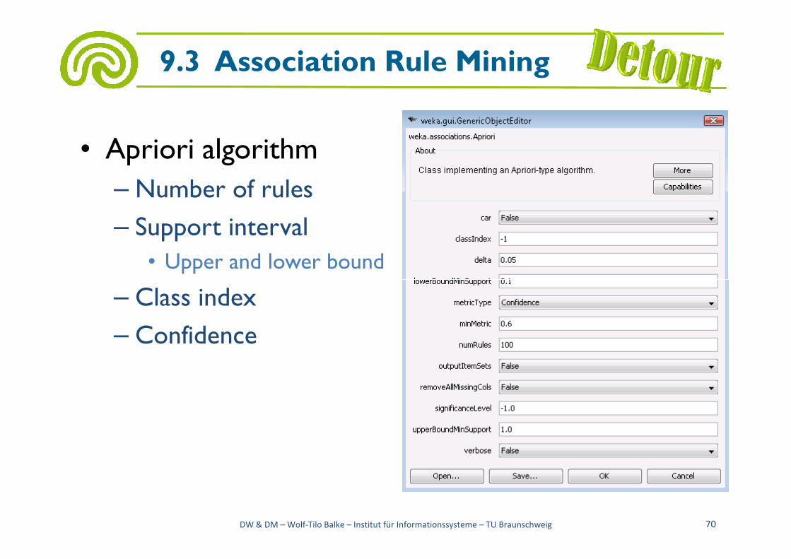
• Apriori algorithm

– Number of rules

– Support interval

• Upper and lower bound


– Class index

– Confidence


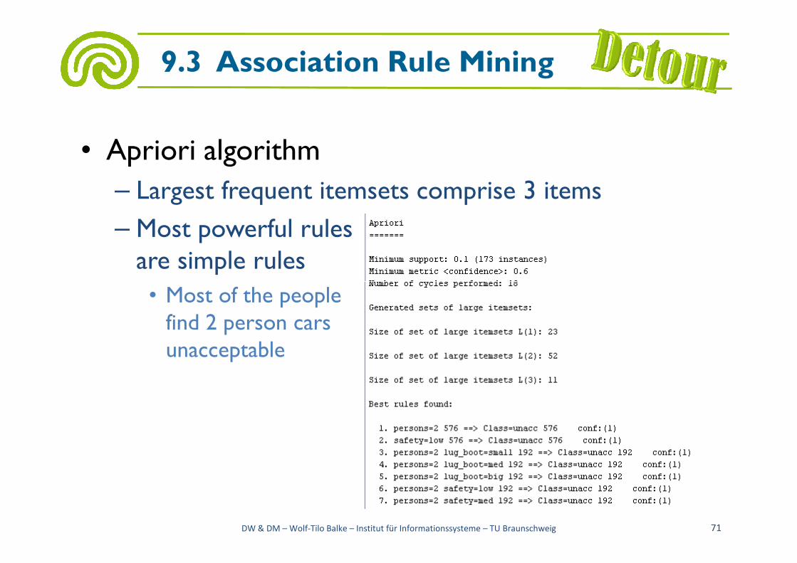
• Apriori algorithm

– Largest frequent itemsets comprise 3 items

– Most powerful rulesare simple rules

Most of the people


• Most of the peoplefind 2 person carsunacceptable


– Lower confidence rule (62%)

• Unacceptable, 4 seatcar, is probably unsafe(rule 30)



• Open source projects also have their limits

– Car accidents data set

• 350 000 rows

• 54 attributes



• Data Mining

– Time Series data

• Trend and Similarity Search Analysis

– Sequence Patterns

Next lecture


data warehousing & data mining - tu · pdf filedata warehousing & data mining...

Documents