database theory - lecture 12: evaluation of datalog (2) · pdf filedatabase theory lecture 12:...
TRANSCRIPT
DATABASE THEORY
Lecture 12: Evaluation of Datalog (2)
Markus Krotzsch
TU Dresden, 30 June 2016
Overview1. Introduction | Relational data model2. First-order queries3. Complexity of query answering4. Complexity of FO query answering5. Conjunctive queries6. Tree-like conjunctive queries7. Query optimisation8. Conjunctive Query Optimisation / First-Order Expressiveness9. First-Order Expressiveness / Introduction to Datalog
10. Expressive Power and Complexity of Datalog11. Optimisation and Evaluation of Datalog12. Evaluation of Datalog (2)13. Graph Databases and Path Queries14. Outlook: database theory in practice
See course homepage [⇒ link] for more information and materialsMarkus Krötzsch, 30 June 2016 Database Theory slide 2 of 43

Review: Datalog Evaluation
A rule-based recursive query language
father(alice, bob)
mother(alice, carla)
Parent(x, y)← father(x, y)
Parent(x, y)← mother(x, y)
SameGeneration(x, x)
SameGeneration(x, y)← Parent(x, v) ∧ Parent(y, w) ∧ SameGeneration(v, w)
Perfect static optimisation for Datalog is undecidable
Datalog queries can be evaluated bottom-up or top-down
Simplest practical bottom-up technique: semi-naive evaluation
Markus Krötzsch, 30 June 2016 Database Theory slide 3 of 43

Semi-Naive Evaluation: Example
e(1, 2) e(2, 3) e(3, 4) e(4, 5)
(R1) T(x, y)← e(x, y)
(R2.1) T(x, z)← ∆iT(x, y) ∧ Ti(y, z)
(R2.2′) T(x, z)← Ti−1(x, y) ∧ ∆iT(y, z)
How many body matches do we need to iterate over?
T0P = ∅ initialisation
T1P = {T(1, 2), T(2, 3), T(3, 4), T(4, 5)} 4 × (R1)
T2P = T1
P ∪ {T(1, 3), T(2, 4), T(3, 5)} 3 × (R2.1)
T3P = T2
P ∪ {T(1, 4), T(2, 5), T(1, 5)} 3 × (R2.1), 2 × (R2.2′)
T4P = T3
P = T∞P 1 × (R2.1), 1 × (R2.2′)
In total, we considered 14 matches to derive 11 factsMarkus Krötzsch, 30 June 2016 Database Theory slide 4 of 43

Semi-Naive Evaluation: Full DefinitionIn general, a rule of the form
H(~x)← e1(~y1) ∧ . . . ∧ en(~yn) ∧ I1(~z1) ∧ I2(~z2) ∧ . . . ∧ Im(~zm)
is transformed into m rules
H(~x)← e1(~y1) ∧ . . . ∧ en(~yn) ∧ ∆iI1 (~z1) ∧ Ii2(~z2) ∧ . . . ∧ Iim(~zm)
H(~x)← e1(~y1) ∧ . . . ∧ en(~yn) ∧ Ii−11 (~z1) ∧ ∆i
I2 (~z2) ∧ . . . ∧ Iim(~zm)
. . .
H(~x)← e1(~y1) ∧ . . . ∧ en(~yn) ∧ Ii−11 (~z1) ∧ Ii−1
2 (~z2) ∧ . . . ∧ ∆iIm (~zm)
Advantages and disadvantages:
• Huge improvement over naive evaluation
• Some redundant computations remain (see example)
• Some overhead for implementation (store level of entailments)
Markus Krötzsch, 30 June 2016 Database Theory slide 5 of 43
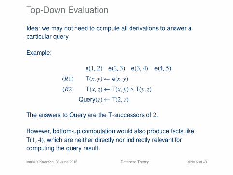
Top-Down Evaluation
Idea: we may not need to compute all derivations to answer aparticular query
Example:
e(1, 2) e(2, 3) e(3, 4) e(4, 5)
(R1) T(x, y)← e(x, y)
(R2) T(x, z)← T(x, y) ∧ T(y, z)
Query(z)← T(2, z)
The answers to Query are the T-successors of 2.
However, bottom-up computation would also produce facts likeT(1, 4), which are neither directly nor indirectly relevant forcomputing the query result.
Markus Krötzsch, 30 June 2016 Database Theory slide 6 of 43

Assumption
For all techniques presented in this lecture, we assume that thegiven Datalog program is safe.
• This is without loss of generality (as shown in exercise).
• One can avoid this by adding more cases to algorithms.
Markus Krötzsch, 30 June 2016 Database Theory slide 7 of 43
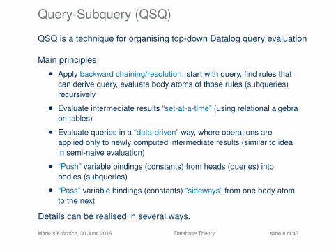
Query-Subquery (QSQ)
QSQ is a technique for organising top-down Datalog query evaluation
Main principles:• Apply backward chaining/resolution: start with query, find rules that
can derive query, evaluate body atoms of those rules (subqueries)recursively
• Evaluate intermediate results “set-at-a-time” (using relational algebraon tables)
• Evaluate queries in a “data-driven” way, where operations areapplied only to newly computed intermediate results (similar to ideain semi-naive evaluation)
• “Push” variable bindings (constants) from heads (queries) intobodies (subqueries)
• “Pass” variable bindings (constants) “sideways” from one body atomto the next
Details can be realised in several ways.
Markus Krötzsch, 30 June 2016 Database Theory slide 8 of 43

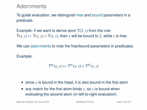
AdornmentsTo guide evaluation, we distinguish free and bound parameters in apredicate.
Example: if we want to derive atom T(2, z) from the ruleT(x, z)← T(x, y) ∧ T(y, z), then x will be bound to 2, while z is free.
We use adornments to note the free/bound parameters in predicates.
Example:
Tbf (x, z)← Tbf (x, y) ∧ Tbf (y, z)
• since x is bound in the head, it is also bound in the first atom
• any match for the first atom binds y, so y is bound whenevaluating the second atom (in left-to-right evaluation)
Markus Krötzsch, 30 June 2016 Database Theory slide 9 of 43
AdornmentsTo guide evaluation, we distinguish free and bound parameters in apredicate.
Example: if we want to derive atom T(2, z) from the ruleT(x, z)← T(x, y) ∧ T(y, z), then x will be bound to 2, while z is free.
We use adornments to note the free/bound parameters in predicates.
Example:
Tbf (x, z)← Tbf (x, y) ∧ Tbf (y, z)
• since x is bound in the head, it is also bound in the first atom
• any match for the first atom binds y, so y is bound whenevaluating the second atom (in left-to-right evaluation)
Markus Krötzsch, 30 June 2016 Database Theory slide 10 of 43

Adornments: Examples
The adornment of the head of a rule determines the adornments ofthe body atoms:
Rbbb(x, y, z)← Rbbf (x, y, v) ∧ Rbbb(x, v, z)
Rfbf (x, y, z)← Rfbf (x, y, v) ∧ Rbbf (x, v, z)
The order of body predicates matters affects the adornment:
Sfff (x, y, z)← Tff (x, v) ∧ Tff (y, w) ∧ Rbbf (v, w, z)
Sfff (x, y, z)← Rfff (v, w, z) ∧ Tfb(x, v) ∧ Tfb(y, w)
{ For optimisation, some orders might be better than others
Markus Krötzsch, 30 June 2016 Database Theory slide 11 of 43

Adornments: Examples
The adornment of the head of a rule determines the adornments ofthe body atoms:
Rbbb(x, y, z)← Rbbf (x, y, v) ∧ Rbbb(x, v, z)
Rfbf (x, y, z)← Rfbf (x, y, v) ∧ Rbbf (x, v, z)
The order of body predicates matters affects the adornment:
Sfff (x, y, z)← Tff (x, v) ∧ Tff (y, w) ∧ Rbbf (v, w, z)
Sfff (x, y, z)← Rfff (v, w, z) ∧ Tfb(x, v) ∧ Tfb(y, w)
{ For optimisation, some orders might be better than others
Markus Krötzsch, 30 June 2016 Database Theory slide 12 of 43
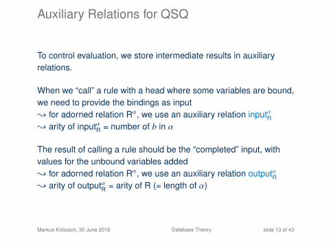
Auxiliary Relations for QSQ
To control evaluation, we store intermediate results in auxiliaryrelations.
When we “call” a rule with a head where some variables are bound,we need to provide the bindings as input{ for adorned relation Rα, we use an auxiliary relation inputαR{ arity of inputαR = number of b in α
The result of calling a rule should be the “completed” input, withvalues for the unbound variables added{ for adorned relation Rα, we use an auxiliary relation outputαR{ arity of outputαR = arity of R (= length of α)
Markus Krötzsch, 30 June 2016 Database Theory slide 13 of 43

Auxiliary Relations for QSQ (2)When evaluating body atoms from left to right, we usesupplementary relations supi
{ bindings required to evaluate rest of rule after the ith body atom{ the first set of bindings sup0 comes from inputαR{ the last set of bindings supn go to outputαR
Example:
Tbf (x, z)← Tbf (x, y) ∧ Tbf (y, z)⇑ u ⇑ u
inputbfT ⇒ sup0[x] sup1[x, y] sup2[x, z]⇒ outputbf
T
• sup0[x] is copied from inputbfT [x] (with some exceptions, see exercise)
• sup1[x, y] is obtained by joining tables sup0[x] and outputbfT [x, y]
• sup2[x, z] is obtained by joining tables sup1[x, y] and outputbfT [y, z]
• outputbfT [x, z] is copied from sup2[x, z]
(we use “named” notation like [x, y] to suggest what to join on; the relations are the same)
Markus Krötzsch, 30 June 2016 Database Theory slide 14 of 43

Auxiliary Relations for QSQ (2)When evaluating body atoms from left to right, we usesupplementary relations supi
{ bindings required to evaluate rest of rule after the ith body atom{ the first set of bindings sup0 comes from inputαR{ the last set of bindings supn go to outputαR
Example:
Tbf (x, z)← Tbf (x, y) ∧ Tbf (y, z)⇑ u ⇑ u
inputbfT ⇒ sup0[x] sup1[x, y] sup2[x, z]⇒ outputbf
T
• sup0[x] is copied from inputbfT [x] (with some exceptions, see exercise)
• sup1[x, y] is obtained by joining tables sup0[x] and outputbfT [x, y]
• sup2[x, z] is obtained by joining tables sup1[x, y] and outputbfT [y, z]
• outputbfT [x, z] is copied from sup2[x, z]
(we use “named” notation like [x, y] to suggest what to join on; the relations are the same)
Markus Krötzsch, 30 June 2016 Database Theory slide 15 of 43

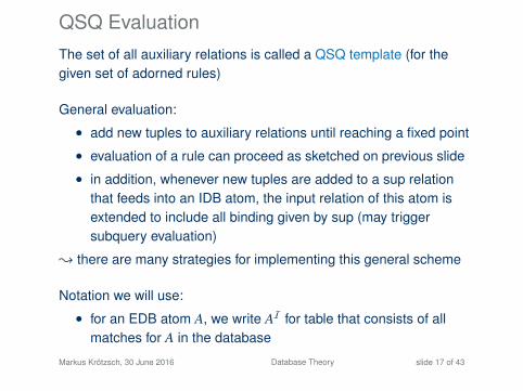
QSQ EvaluationThe set of all auxiliary relations is called a QSQ template (for thegiven set of adorned rules)
General evaluation:
• add new tuples to auxiliary relations until reaching a fixed point
• evaluation of a rule can proceed as sketched on previous slide
• in addition, whenever new tuples are added to a sup relationthat feeds into an IDB atom, the input relation of this atom isextended to include all binding given by sup (may triggersubquery evaluation)
{ there are many strategies for implementing this general scheme
Notation we will use:
• for an EDB atom A, we write AI for table that consists of allmatches for A in the database
Markus Krötzsch, 30 June 2016 Database Theory slide 16 of 43
QSQ EvaluationThe set of all auxiliary relations is called a QSQ template (for thegiven set of adorned rules)
General evaluation:
• add new tuples to auxiliary relations until reaching a fixed point
• evaluation of a rule can proceed as sketched on previous slide
• in addition, whenever new tuples are added to a sup relationthat feeds into an IDB atom, the input relation of this atom isextended to include all binding given by sup (may triggersubquery evaluation)
{ there are many strategies for implementing this general scheme
Notation we will use:
• for an EDB atom A, we write AI for table that consists of allmatches for A in the database
Markus Krötzsch, 30 June 2016 Database Theory slide 17 of 43
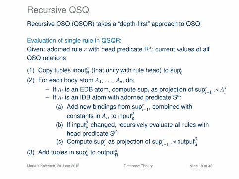
Recursive QSQRecursive QSQ (QSQR) takes a “depth-first” approach to QSQ
Evaluation of single rule in QSQR:Given: adorned rule r with head predicate Rα; current values of allQSQ relations
(1) Copy tuples inputαR (that unify with rule head) to supr0
(2) For each body atom A1, . . . , An, do:– If Ai is an EDB atom, compute supi as projection of supr
i−1 ./ AIi– If Ai is an IDB atom with adorned predicate Sβ:
(a) Add new bindings from supri−1, combined with
constants in Ai, to inputβS(b) If inputβS changed, recursively evaluate all rules with
head predicate Sβ
(c) Compute supri as projection of supr
i−1 ./ outputβS(3) Add tuples in supr
n to outputαR
Markus Krötzsch, 30 June 2016 Database Theory slide 18 of 43
QSQR Algorithm
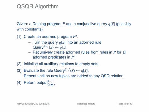
Given: a Datalog program P and a conjunctive query q[~x] (possiblywith constants)
(1) Create an adorned program Pa:– Turn the query q[~x] into an adorned rule
Queryff ...f (~x)← q[~x]– Recursively create adorned rules from rules in P for all
adorned predicates in Pa.
(2) Initialise all auxiliary relations to empty sets.
(3) Evaluate the rule Queryff ...f (~x)← q[~x].Repeat until no new tuples are added to any QSQ relation.
(4) Return outputff ...fQuery
Markus Krötzsch, 30 June 2016 Database Theory slide 19 of 43

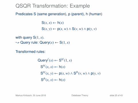
QSQR Transformation: ExamplePredicates S (same generation), p (parent), h (human)
S(x, x)← h(x)
S(x, y)← p(x, w) ∧ S(v, w) ∧ p(y, v)
with query S(1, x).
{ Query rule: Query(x)← S(1, x)
Transformed rules:
Queryf (x)← Sbf (1, x)
Sbf (x, x)← h(x)
Sbf (x, y)← p(x, w) ∧ Sfb(v, w) ∧ p(y, v)
Sfb(x, x)← h(x)
Sfb(x, y)← p(x, w) ∧ Sfb(v, w) ∧ p(y, v)
Markus Krötzsch, 30 June 2016 Database Theory slide 20 of 43

QSQR Transformation: ExamplePredicates S (same generation), p (parent), h (human)
S(x, x)← h(x)
S(x, y)← p(x, w) ∧ S(v, w) ∧ p(y, v)
with query S(1, x).{ Query rule: Query(x)← S(1, x)
Transformed rules:
Queryf (x)← Sbf (1, x)
Sbf (x, x)← h(x)
Sbf (x, y)← p(x, w) ∧ Sfb(v, w) ∧ p(y, v)
Sfb(x, x)← h(x)
Sfb(x, y)← p(x, w) ∧ Sfb(v, w) ∧ p(y, v)
Markus Krötzsch, 30 June 2016 Database Theory slide 21 of 43

QSQR Transformation: ExamplePredicates S (same generation), p (parent), h (human)
S(x, x)← h(x)
S(x, y)← p(x, w) ∧ S(v, w) ∧ p(y, v)
with query S(1, x).{ Query rule: Query(x)← S(1, x)
Transformed rules:
Queryf (x)← Sbf (1, x)
Sbf (x, x)← h(x)
Sbf (x, y)← p(x, w) ∧ Sfb(v, w) ∧ p(y, v)
Sfb(x, x)← h(x)
Sfb(x, y)← p(x, w) ∧ Sfb(v, w) ∧ p(y, v)
Markus Krötzsch, 30 June 2016 Database Theory slide 22 of 43

QSQR Transformation: ExamplePredicates S (same generation), p (parent), h (human)
S(x, x)← h(x)
S(x, y)← p(x, w) ∧ S(v, w) ∧ p(y, v)
with query S(1, x).{ Query rule: Query(x)← S(1, x)
Transformed rules:
Queryf (x)← Sbf (1, x)
Sbf (x, x)← h(x)
Sbf (x, y)← p(x, w) ∧ Sfb(v, w) ∧ p(y, v)
Sfb(x, x)← h(x)
Sfb(x, y)← p(x, w) ∧ Sfb(v, w) ∧ p(y, v)
Markus Krötzsch, 30 June 2016 Database Theory slide 23 of 43

QSQR Transformation: ExamplePredicates S (same generation), p (parent), h (human)
S(x, x)← h(x)
S(x, y)← p(x, w) ∧ S(v, w) ∧ p(y, v)
with query S(1, x).{ Query rule: Query(x)← S(1, x)
Transformed rules:
Queryf (x)← Sbf (1, x)
Sbf (x, x)← h(x)
Sbf (x, y)← p(x, w) ∧ Sfb(v, w) ∧ p(y, v)
Sfb(x, x)← h(x)
Sfb(x, y)← p(x, w) ∧ Sfb(v, w) ∧ p(y, v)
Markus Krötzsch, 30 June 2016 Database Theory slide 24 of 43
QSQR Transformation: ExamplePredicates S (same generation), p (parent), h (human)
S(x, x)← h(x)
S(x, y)← p(x, w) ∧ S(v, w) ∧ p(y, v)
with query S(1, x).{ Query rule: Query(x)← S(1, x)
Transformed rules:
Queryf (x)← Sbf (1, x)
Sbf (x, x)← h(x)
Sbf (x, y)← p(x, w) ∧ Sfb(v, w) ∧ p(y, v)
Sfb(x, x)← h(x)
Sfb(x, y)← p(x, w) ∧ Sfb(v, w) ∧ p(y, v)
Markus Krötzsch, 30 June 2016 Database Theory slide 25 of 43

QSQR Transformation: ExamplePredicates S (same generation), p (parent), h (human)
S(x, x)← h(x)
S(x, y)← p(x, w) ∧ S(v, w) ∧ p(y, v)
with query S(1, x).{ Query rule: Query(x)← S(1, x)
Transformed rules:
Queryf (x)← Sbf (1, x)
Sbf (x, x)← h(x)
Sbf (x, y)← p(x, w) ∧ Sfb(v, w) ∧ p(y, v)
Sfb(x, x)← h(x)
Sfb(x, y)← p(x, w) ∧ Sfb(v, w) ∧ p(y, v)
Markus Krötzsch, 30 June 2016 Database Theory slide 26 of 43
Magic Sets
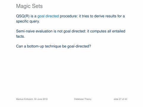
QSQ(R) is a goal directed procedure: it tries to derive results for aspecific query.
Semi-naive evaluation is not goal directed: it computes all entailedfacts.
Can a bottom-up technique be goal-directed?
{ yes, by magic
Magic Sets
• “Simulation” of QSQ by Datalog rules
• Can be evaluated bottom up, e.g., with semi-naive evaluation
• The “magic sets” are the sets of tuples stored in the auxiliaryrelations
• Several other variants of the method exist
Markus Krötzsch, 30 June 2016 Database Theory slide 27 of 43

Magic Sets
QSQ(R) is a goal directed procedure: it tries to derive results for aspecific query.
Semi-naive evaluation is not goal directed: it computes all entailedfacts.
Can a bottom-up technique be goal-directed?{ yes, by magic
Magic Sets
• “Simulation” of QSQ by Datalog rules
• Can be evaluated bottom up, e.g., with semi-naive evaluation
• The “magic sets” are the sets of tuples stored in the auxiliaryrelations
• Several other variants of the method exist
Markus Krötzsch, 30 June 2016 Database Theory slide 28 of 43

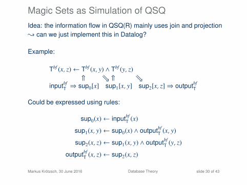
Magic Sets as Simulation of QSQIdea: the information flow in QSQ(R) mainly uses join and projection{ can we just implement this in Datalog?
Example:
Tbf (x, z)← Tbf (x, y) ∧ Tbf (y, z)⇑ u ⇑ u
inputbfT ⇒ sup0[x] sup1[x, y] sup2[x, z]⇒ outputbf
T
Could be expressed using rules:
sup0(x)← inputbfT (x)
sup1(x, y)← sup0(x) ∧ outputbfT (x, y)
sup2(x, z)← sup1(x, y) ∧ outputbfT (y, z)
outputbfT (x, z)← sup2(x, z)
Markus Krötzsch, 30 June 2016 Database Theory slide 29 of 43
Magic Sets as Simulation of QSQIdea: the information flow in QSQ(R) mainly uses join and projection{ can we just implement this in Datalog?
Example:
Tbf (x, z)← Tbf (x, y) ∧ Tbf (y, z)⇑ u ⇑ u
inputbfT ⇒ sup0[x] sup1[x, y] sup2[x, z]⇒ outputbf
T
Could be expressed using rules:
sup0(x)← inputbfT (x)
sup1(x, y)← sup0(x) ∧ outputbfT (x, y)
sup2(x, z)← sup1(x, y) ∧ outputbfT (y, z)
outputbfT (x, z)← sup2(x, z)
Markus Krötzsch, 30 June 2016 Database Theory slide 30 of 43

Magic Sets as Simulation of QSQ (2)
Observation: sup0(x) and sup2(x, z) are redundant. Simpler:
sup1(x, y)← inputbfT (x) ∧ outputbf
T (x, y)
outputbfT (x, z)← sup1(x, y) ∧ outputbf
T (y, z)
We still need to “call” subqueries recursively:
inputbfT (y)← sup1(x, y)
It is easy to see how to do this for arbitrary adorned rules.
Markus Krötzsch, 30 June 2016 Database Theory slide 31 of 43

A Note on Constants
Constants in rule bodies must lead to bindings in the subquery.
Example: the following rule is correctly adorned
Rbf (x, y)← Tbbf (x, a, z)
This leads to the following rules using Magic Sets:
outputbfR (x, y)← inputbf
R (x) ∧ outputbfbT (x, a, y)
inputbbfT (x, a)← inputbf
R (x)
Note that we do not need to use auxiliary predicates sup0 or sup1 here, bythe simplification on the previous slide.
Markus Krötzsch, 30 June 2016 Database Theory slide 32 of 43

A Note on Constants
Constants in rule bodies must lead to bindings in the subquery.
Example: the following rule is correctly adorned
Rbf (x, y)← Tbbf (x, a, z)
This leads to the following rules using Magic Sets:
outputbfR (x, y)← inputbf
R (x) ∧ outputbfbT (x, a, y)
inputbbfT (x, a)← inputbf
R (x)
Note that we do not need to use auxiliary predicates sup0 or sup1 here, bythe simplification on the previous slide.
Markus Krötzsch, 30 June 2016 Database Theory slide 33 of 43

Magic Sets: Summary
A goal-directed bottom-up technique:
• Rewritten program rules can be constructed on the fly
• Bottom-up evaluation can be semi-naive (avoid repeated ruleapplications)
• Supplementary relations can be cached in between queries
Nevertheless, a full materialisation might be better, if
• Database does not change very often (materialisation asone-time investment)
• Queries are very diverse and may use any IDB relation (badfor caching supplementary relations)
{ semi-naive evaluation is still very common in practice
Markus Krötzsch, 30 June 2016 Database Theory slide 34 of 43

Magic Sets: Summary
A goal-directed bottom-up technique:
• Rewritten program rules can be constructed on the fly
• Bottom-up evaluation can be semi-naive (avoid repeated ruleapplications)
• Supplementary relations can be cached in between queries
Nevertheless, a full materialisation might be better, if
• Database does not change very often (materialisation asone-time investment)
• Queries are very diverse and may use any IDB relation (badfor caching supplementary relations)
{ semi-naive evaluation is still very common in practice
Markus Krötzsch, 30 June 2016 Database Theory slide 35 of 43

Datalog as a Special Case
Datalog is a special case of many approaches, leading to verydiverse implementation techniques.
• Prolog is essentially “Datalog with function symbols” (andmany built-ins).
• Answer Set Programming is “Datalog extended withnon-monotonic negation and disjunction”
• Production Rules use “bottom-up rule reasoning withoperational, non-monotonic built-ins”
• Recursive SQL Queries are a syntactically restricted set ofDatalog rules
{ Different scenarios, different optimal solutions{ Not all implementations are complete (e.g., Prolog)
Markus Krötzsch, 30 June 2016 Database Theory slide 36 of 43

Datalog as a Special Case
Datalog is a special case of many approaches, leading to verydiverse implementation techniques.
• Prolog is essentially “Datalog with function symbols” (andmany built-ins).
• Answer Set Programming is “Datalog extended withnon-monotonic negation and disjunction”
• Production Rules use “bottom-up rule reasoning withoperational, non-monotonic built-ins”
• Recursive SQL Queries are a syntactically restricted set ofDatalog rules
{ Different scenarios, different optimal solutions{ Not all implementations are complete (e.g., Prolog)
Markus Krötzsch, 30 June 2016 Database Theory slide 37 of 43
Datalog as a Special Case
Datalog is a special case of many approaches, leading to verydiverse implementation techniques.
• Prolog is essentially “Datalog with function symbols” (andmany built-ins).
• Answer Set Programming is “Datalog extended withnon-monotonic negation and disjunction”
• Production Rules use “bottom-up rule reasoning withoperational, non-monotonic built-ins”
• Recursive SQL Queries are a syntactically restricted set ofDatalog rules
{ Different scenarios, different optimal solutions{ Not all implementations are complete (e.g., Prolog)
Markus Krötzsch, 30 June 2016 Database Theory slide 38 of 43

Datalog as a Special Case
Datalog is a special case of many approaches, leading to verydiverse implementation techniques.
• Prolog is essentially “Datalog with function symbols” (andmany built-ins).
• Answer Set Programming is “Datalog extended withnon-monotonic negation and disjunction”
• Production Rules use “bottom-up rule reasoning withoperational, non-monotonic built-ins”
• Recursive SQL Queries are a syntactically restricted set ofDatalog rules
{ Different scenarios, different optimal solutions{ Not all implementations are complete (e.g., Prolog)
Markus Krötzsch, 30 June 2016 Database Theory slide 39 of 43
Datalog as a Special Case
Datalog is a special case of many approaches, leading to verydiverse implementation techniques.
• Prolog is essentially “Datalog with function symbols” (andmany built-ins).
• Answer Set Programming is “Datalog extended withnon-monotonic negation and disjunction”
• Production Rules use “bottom-up rule reasoning withoperational, non-monotonic built-ins”
• Recursive SQL Queries are a syntactically restricted set ofDatalog rules
{ Different scenarios, different optimal solutions{ Not all implementations are complete (e.g., Prolog)
Markus Krötzsch, 30 June 2016 Database Theory slide 40 of 43

Datalog as a Special Case
Datalog is a special case of many approaches, leading to verydiverse implementation techniques.
• Prolog is essentially “Datalog with function symbols” (andmany built-ins).
• Answer Set Programming is “Datalog extended withnon-monotonic negation and disjunction”
• Production Rules use “bottom-up rule reasoning withoperational, non-monotonic built-ins”
• Recursive SQL Queries are a syntactically restricted set ofDatalog rules
{ Different scenarios, different optimal solutions{ Not all implementations are complete (e.g., Prolog)
Markus Krötzsch, 30 June 2016 Database Theory slide 41 of 43

Datalog Implementation in Practice
Dedicated Datalog engines as of 2015:
• DLV Answer set programming engine with good performanceon Datalog programs (commercial)
• LogicBlox Big data analytics platform that uses Datalog rules(commercial)
• Datomic Distributed, versioned database using Datalog asmain query language (commercial)
Several RDF (graph data model) DBMS also support Datalog-likerules, usually with limited IDB arity, e.g.:
• OWLIM Disk-backed RDF database with materialisation atload time (commercial)
• RDFox Fast in-memory RDF database with runtimematerialisation and updates (academic)
{ Extremely diverse tools for very different requirements
Markus Krötzsch, 30 June 2016 Database Theory slide 42 of 43

Summary and Outlook
Several implementation techniques for Datalog
• bottom up (from the data) or top down (from the query)
• goal-directed (for a query) or not
Top-down: Query-Subquery (QSQ) approach (goal-directed)
Bottom-up:
• naive evaluation (not goal-directed)
• semi-naive evaluation (not goal-directed)
• Magic Sets (goal-directed)
Next topics:
• Graph databases and path queries
• Applications
Markus Krötzsch, 30 June 2016 Database Theory slide 43 of 43