Databases 101 & Multimedia Support

Joe HellersteinComputer Science Division

UC Berkeley

Overview for the day

• Databases 101– Motivation– Relational databases– Relational Algebra & SQL– Functional units in a DBMS Engine

• Indexes and Query Optimizers

• MM Objects in a DBMS– ADT support– GiST & multi-d indexing– Similarity Search and MM indexing

What we’re skipping• Concurrency and Recovery

– How DBs ensure your data is safe, despite concurrent access and crashes

• Buffer Management– How to manage a main-mem cache, and still guarantee

correctness in the face of crashes• Query optimization

– how to map a declarative query (SQL) to a query plan (relational algebra + implementations)

• Query processing algorithms– sort, hash, join algorithms

• Database design– logical design: E-R models & normalization– physical design: indexes, clustering, tuning

More Background• Overview Texts:

– Ramakrishnan, Database Management Systems (the cow book)

– Silberschatz, Korth, Sudarshan: Database System Concepts (the sailboat book)

– O’Neil: Database Principles, Programming, Performance– Ullman & Widom: A 1st Course in Database Systems

• Graduate-level Texts– Stonebraker & Hellerstein, eds. Readings in Database

Systems (http://redbook.cs.berkeley.edu)– Gray & Reuter: Transaction Processing: Concepts and

Techniques.– Ullman: Principles of Database Systems– Faloutsos: Searching Multimedia Databases by Content

Database Management Systems• What more could we want than a file

system?– Simple, efficient ad hoc1 queries– concurrency control– recovery– benefits of good data modeling

1ad hoc: formed or used for specific or immediate problems or needs

Describing Data: Data Models• A data model is a collection of concepts

for describing data.• A schema is a description of a particular

collection of data, using the a given data model.

• The relational model of data is the most widely used model today.– Main concept: relation, basically a table with

rows and columns.– Every relation has a schema, which describes

the columns, or fields.

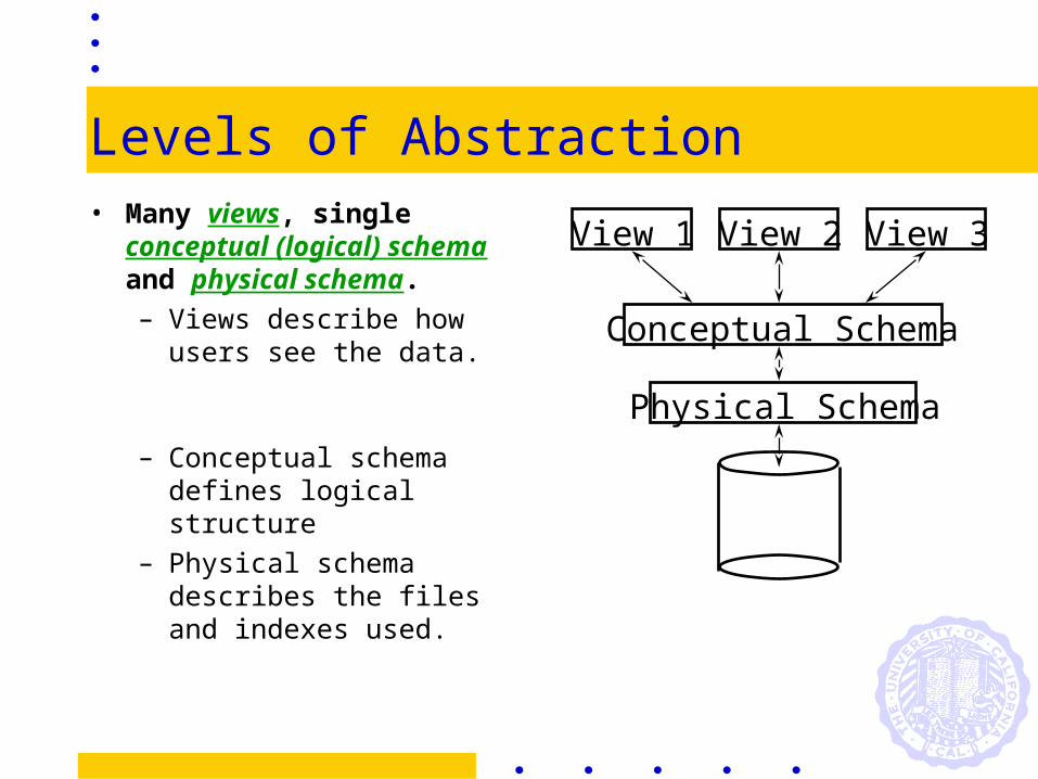
Levels of Abstraction• Many views, single

conceptual (logical) schema and physical schema.– Views describe how

users see the data.

– Conceptual schema defines logical structure

– Physical schema describes the files and indexes used.

Physical Schema

Conceptual Schema

View 1 View 2 View 3

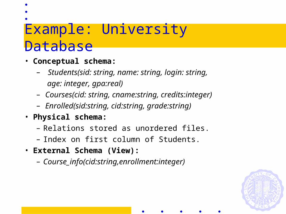
Example: University Database

• Conceptual schema: – Students(sid: string, name: string, login: string,

age: integer, gpa:real)– Courses(cid: string, cname:string, credits:integer) – Enrolled(sid:string, cid:string, grade:string)

• Physical schema:– Relations stored as unordered files. – Index on first column of Students.

• External Schema (View): – Course_info(cid:string,enrollment:integer)

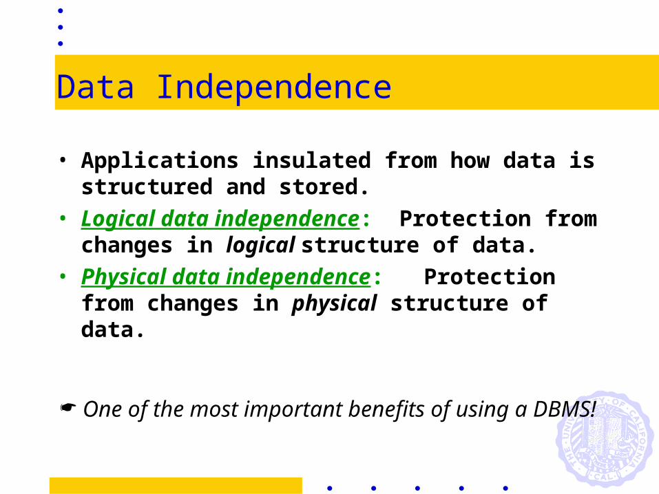
Data Independence

• Applications insulated from how data is structured and stored.

• Logical data independence: Protection from changes in logical structure of data.

• Physical data independence: Protection from changes in physical structure of data.

One of the most important benefits of using a DBMS!

Structure of a DBMS

• A typical DBMS has a layered architecture.

• The figure does not show the concurrency control and recovery components.

• This is one of several possible architectures; each system has its own variations.

Query Optimizationand Execution

Relational Operators

Files and Access Methods

Buffer Management

Disk Space Management

DB

These layersmust considerconcurrencycontrol andrecovery

Advantages of a DBMS• Data independence• Efficient data access• Data integrity & security• Data administration• Concurrent access, crash recovery• Reduced application development time• So why not use them always?

– Can be expensive, complicated to set up and maintain

– This cost & complexity must be offset by need

- Often worth it!

By relieving the brain of all unnecessary work, a good notation sets it free to

concentrate on more advanced problems, and, in effect, increases the mental power of

the race.

-- Alfred North Whitehead (1861 - 1947)

Relational Algebra

Relational Query Languages• Query languages: Allow manipulation and

retrieval of data from a database.• Relational model supports simple, powerful QLs:

– Strong formal foundation based on logic.– Allows for much optimization.

• Query Languages != programming languages!– QLs not expected to be “Turing complete”.– QLs not intended to be used for complex

calculations.– QLs support easy, efficient access to large data sets.

Formal Relational Query LanguagesTwo mathematical Query Languages form

the basis for “real” languages (e.g. SQL), and for implementation:

Relational Algebra: More operational, very useful for representing internal execution plans. (Database byte-code…)

Relational Calculus: Lets users describe what they want, rather than how to compute it. (Non-operational, declarative -- SQL comes from here.)

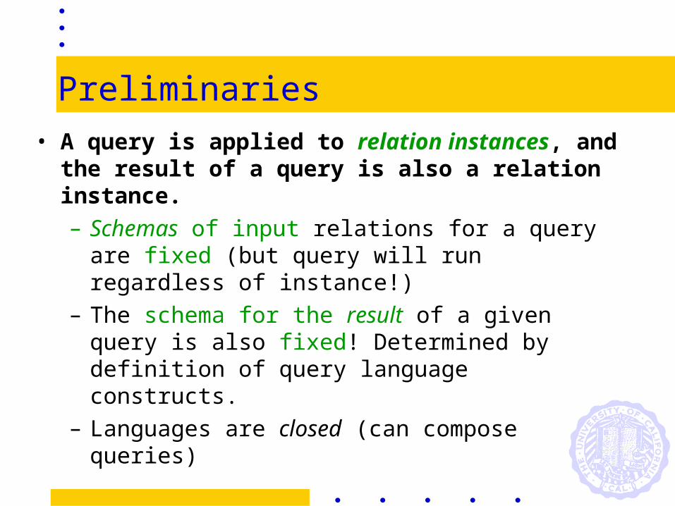
Preliminaries• A query is applied to relation instances, and

the result of a query is also a relation instance.– Schemas of input relations for a query are

fixed (but query will run regardless of instance!)

– The schema for the result of a given query is also fixed! Determined by definition of query language constructs.

– Languages are closed (can compose queries)

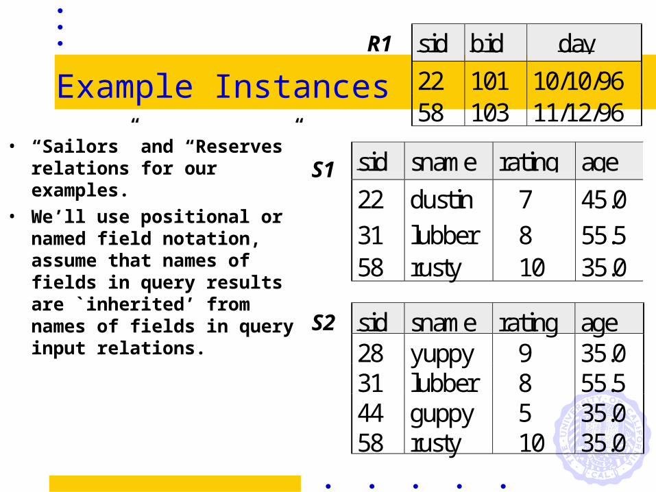
Example Instances

sid sname rating age

22 dustin 7 45.0

31 lubber 8 55.558 rusty 10 35.0

sid sname rating age28 yuppy 9 35.031 lubber 8 55.544 guppy 5 35.058 rusty 10 35.0

sid bid day

22 101 10/10/9658 103 11/12/96

R1

S1

S2

• “Sailors” and “Reserves” relations for our examples.

• We’ll use positional or named field notation, assume that names of fields in query results are `inherited’ from names of fields in query input relations.

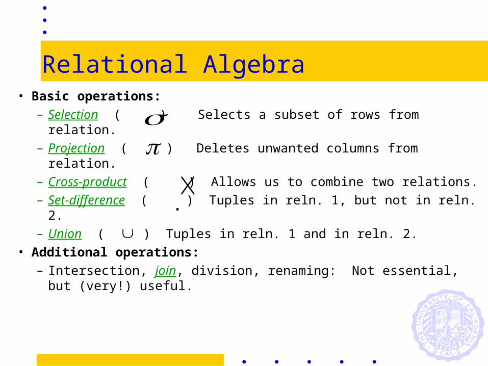
Relational Algebra• Basic operations:

– Selection ( ) Selects a subset of rows from relation.– Projection ( ) Deletes unwanted columns from relation.– Cross-product ( ) Allows us to combine two relations.– Set-difference ( ) Tuples in reln. 1, but not in reln. 2.– Union ( ) Tuples in reln. 1 and in reln. 2.

• Additional operations:– Intersection, join, division, renaming: Not essential, but

(very!) useful.

Projectionsname rating

yuppy 9lubber 8guppy 5rusty 10

sname rating

S,

( )2

age

35.055.5

age S( )2

• Deletes attributes that are not in projection list.

• Schema of result:

– exactly the fields in the projection list, with the same names that they had in the (only) input relation.

• Projection operator has to eliminate duplicates! (Why??)

– Note: real systems typically don’t do duplicate elimination unless the user explicitly asks for it. (Why not?)

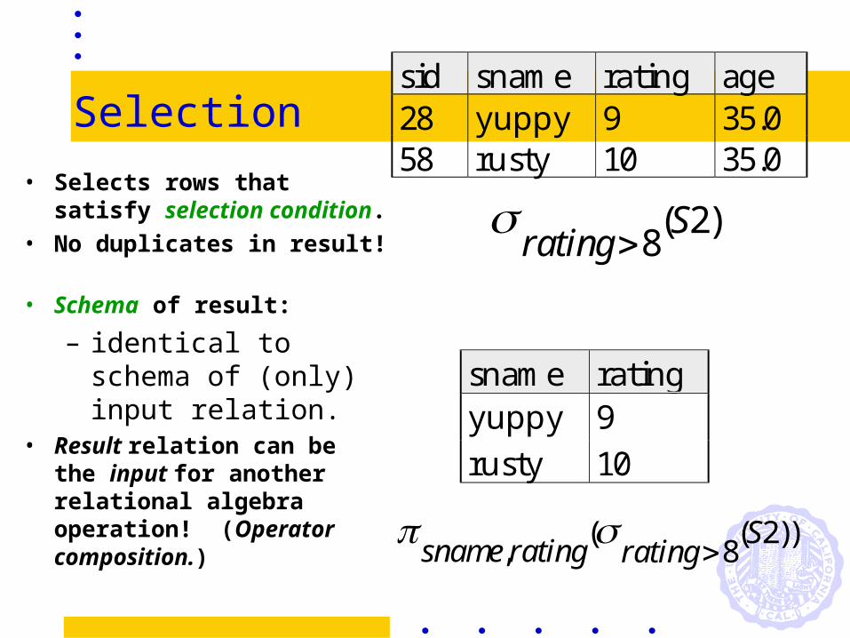
Selection

rating

S8

2( )

sid sname rating age28 yuppy 9 35.058 rusty 10 35.0

sname ratingyuppy 9rusty 10

sname rating rating

S,

( ( ))8

2

• Selects rows that satisfy selection condition.

• No duplicates in result! • Schema of result:

– identical to schema of (only) input relation.

• Result relation can be the input for another relational algebra operation! (Operator composition.)

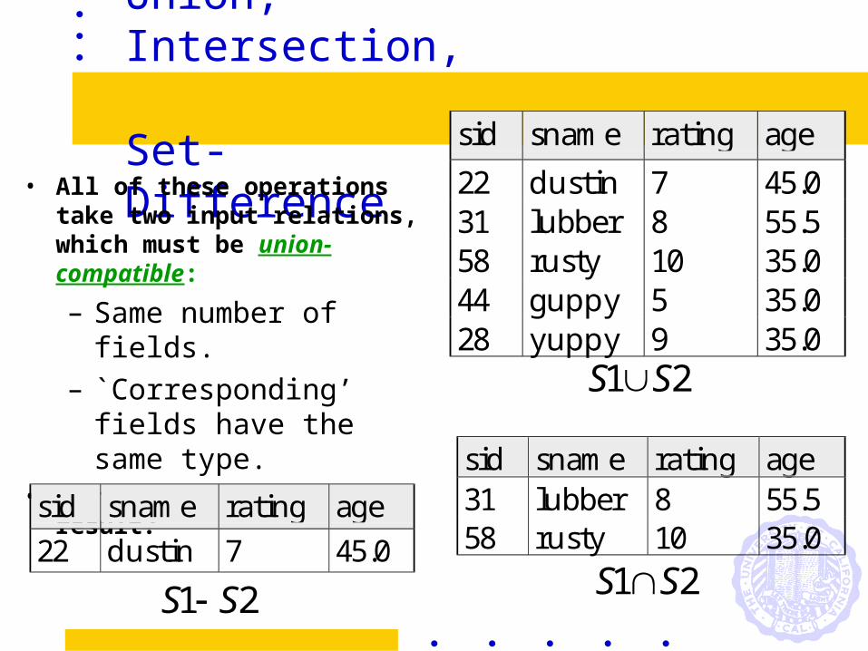
Union, Intersection, Set-Difference

• All of these operations take two input relations, which must be union-compatible:

– Same number of fields.

– `Corresponding’ fields have the same type.

• What is the schema of result?

sid sname rating age

22 dustin 7 45.031 lubber 8 55.558 rusty 10 35.044 guppy 5 35.028 yuppy 9 35.0

sid sname rating age31 lubber 8 55.558 rusty 10 35.0

S S1 2

S S1 2

sid sname rating age

22 dustin 7 45.0

S S1 2

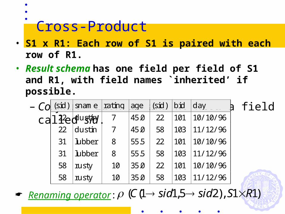
Cross-Product• S1 x R1: Each row of S1 is paired with each

row of R1.• Result schema has one field per field of S1

and R1, with field names `inherited’ if possible.

– Conflict: Both S1 and R1 have a field called sid.

( ( , ), )C sid sid S R1 1 5 2 1 1

(sid) sname rating age (sid) bid day

22 dustin 7 45.0 22 101 10/ 10/ 96

22 dustin 7 45.0 58 103 11/ 12/ 96

31 lubber 8 55.5 22 101 10/ 10/ 96

31 lubber 8 55.5 58 103 11/ 12/ 96

58 rusty 10 35.0 22 101 10/ 10/ 96

58 rusty 10 35.0 58 103 11/ 12/ 96

Renaming operator:

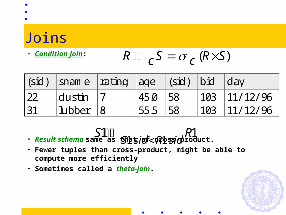
Joins• Condition Join:

• Result schema same as that of cross-product.• Fewer tuples than cross-product, might be able to

compute more efficiently• Sometimes called a theta-join.

R c S c R S ( )

(sid) sname rating age (sid) bid day

22 dustin 7 45.0 58 103 11/ 12/ 9631 lubber 8 55.5 58 103 11/ 12/ 96

11.1.1

RSsidRsidS

Joins• Equi-Join: Special case: condition c contains

only conjunction of equalities.

• Result schema similar to cross-product, but only one copy of fields for which equality is specified.

• Natural Join: Equijoin on all common fields.

sid sname rating age bid day

22 dustin 7 45.0 101 10/ 10/ 9658 rusty 10 35.0 103 11/ 12/ 96

S Rsid

1 1

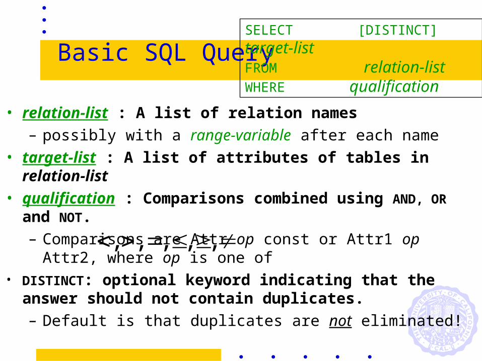
Basic SQL Query

• relation-list : A list of relation names – possibly with a range-variable after each name

• target-list : A list of attributes of tables in relation-list

• qualification : Comparisons combined using AND, OR and NOT.– Comparisons are Attr op const or Attr1 op Attr2,

where op is one of• DISTINCT: optional keyword indicating that the

answer should not contain duplicates. – Default is that duplicates are not eliminated!

SELECT [DISTINCT] target-listFROM relation-listWHERE qualification

, , , , ,

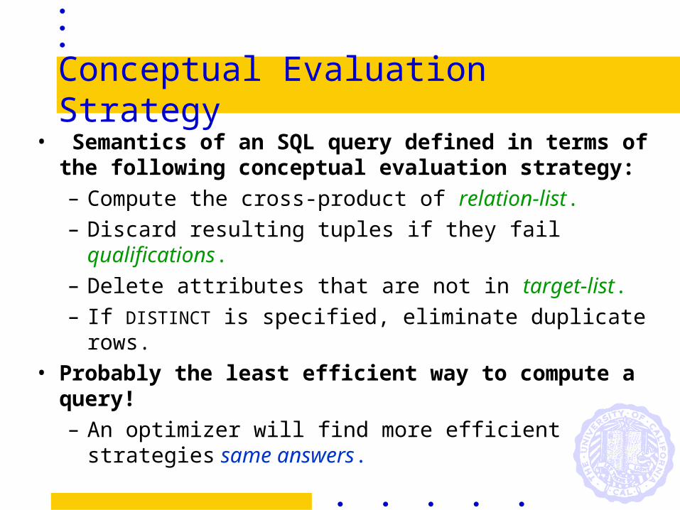
Conceptual Evaluation Strategy• Semantics of an SQL query defined in terms

of the following conceptual evaluation strategy:– Compute the cross-product of relation-list.– Discard resulting tuples if they fail qualifications.– Delete attributes that are not in target-list.– If DISTINCT is specified, eliminate duplicate rows.

• Probably the least efficient way to compute a query! – An optimizer will find more efficient strategies

same answers.

Example of Conceptual EvaluationSELECT S.sname

FROM Sailors S, Reserves RWHERE S.sid=R.sid AND R.bid=103

(sid) sname rating age (sid) bid day

22 dustin 7 45.0 22 101 10/ 10/ 96

22 dustin 7 45.0 58 103 11/ 12/ 96

31 lubber 8 55.5 22 101 10/ 10/ 96

31 lubber 8 55.5 58 103 11/ 12/ 96

58 rusty 10 35.0 22 101 10/ 10/ 96

58 rusty 10 35.0 58 103 11/ 12/ 96

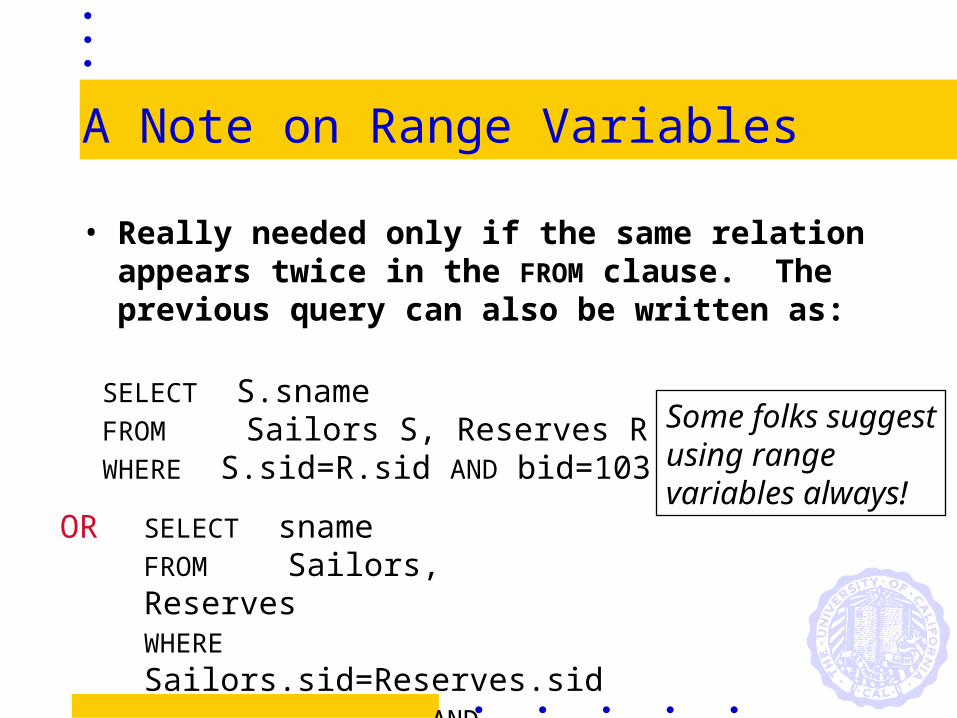
A Note on Range Variables

• Really needed only if the same relation appears twice in the FROM clause. The previous query can also be written as:

SELECT S.snameFROM Sailors S, Reserves RWHERE S.sid=R.sid AND bid=103

SELECT snameFROM Sailors, Reserves WHERE Sailors.sid=Reserves.sid AND bid=103

Some folks suggestusing range variables always!

OR

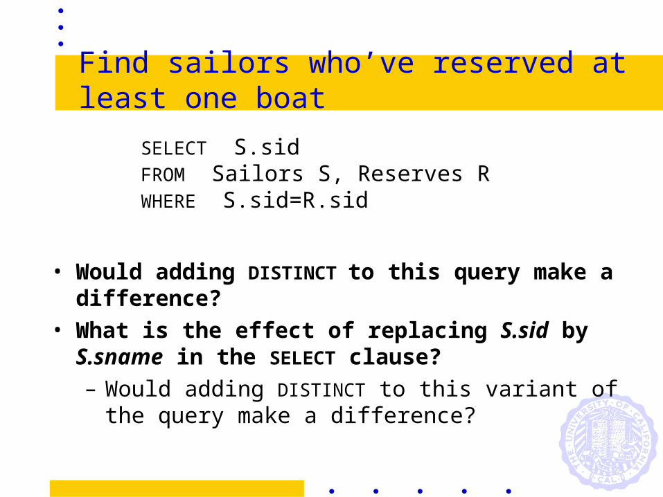
Find sailors who’ve reserved at least one boat

• Would adding DISTINCT to this query make a difference?

• What is the effect of replacing S.sid by S.sname in the SELECT clause? – Would adding DISTINCT to this variant of the

query make a difference?

SELECT S.sidFROM Sailors S, Reserves RWHERE S.sid=R.sid

Expressions and Strings

• Arithmetic expressions, string pattern matching.

• AS and = are two ways to name fields in result.• LIKE is used for string matching.

– `_’ stands for any one character and `%’ stands for 0 or more arbitrary characters.

SELECT S.age, age1=S.age-5, 2*S.age AS age2FROM Sailors SWHERE S.sname LIKE ‘B_%B’

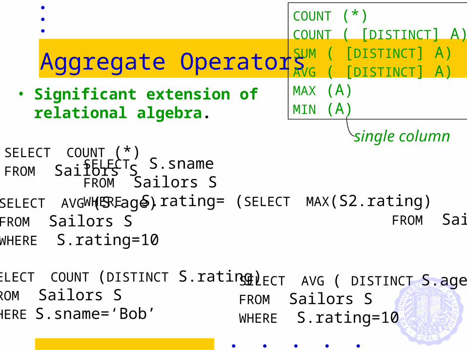
Aggregate Operators• Significant extension of

relational algebra.

COUNT (*)COUNT ( [DISTINCT] A)SUM ( [DISTINCT] A)AVG ( [DISTINCT] A)MAX (A)MIN (A)

SELECT AVG (S.age)FROM Sailors SWHERE S.rating=10

SELECT COUNT (*)FROM Sailors S

SELECT AVG ( DISTINCT S.age)FROM Sailors SWHERE S.rating=10

SELECT S.snameFROM Sailors SWHERE S.rating= (SELECT MAX(S2.rating) FROM Sailors S2)

single column

SELECT COUNT (DISTINCT S.rating)FROM Sailors SWHERE S.sname=‘Bob’

Database APIs: ODBC/JDBC

• special procedures/objects for procedural languages to access DBs– pass SQL strings from language, presents

result sets in a language-friendly way– Microsoft’s ODBC becoming C/C++ standard

on Windows– Sun’s JDBC a Java equivalent– Supposedly DBMS-neutral

• a “driver” traps the calls and translates them into DBMS-specific code

• database can be across a network

SQL API in Java (JDBC)

Connection con = // connect

DriverManager.getConnection(url, ”login", ”pass");

Statement stmt = con.createStatement(); // set up stmt

String query = "SELECT COF_NAME, PRICE FROM COFFEES";

ResultSet rs = stmt.executeQuery(query);

try { // handle exceptions

// loop through result tuples

while (rs.next()) {

String s = rs.getString("COF_NAME");

Float n = rs.getFloat("PRICE");

System.out.println(s + " " + n);

}

} catch(SQLException ex) {

System.out.println(ex.getMessage ()

+ ex.getSQLState () + ex.getErrorCode ());

}

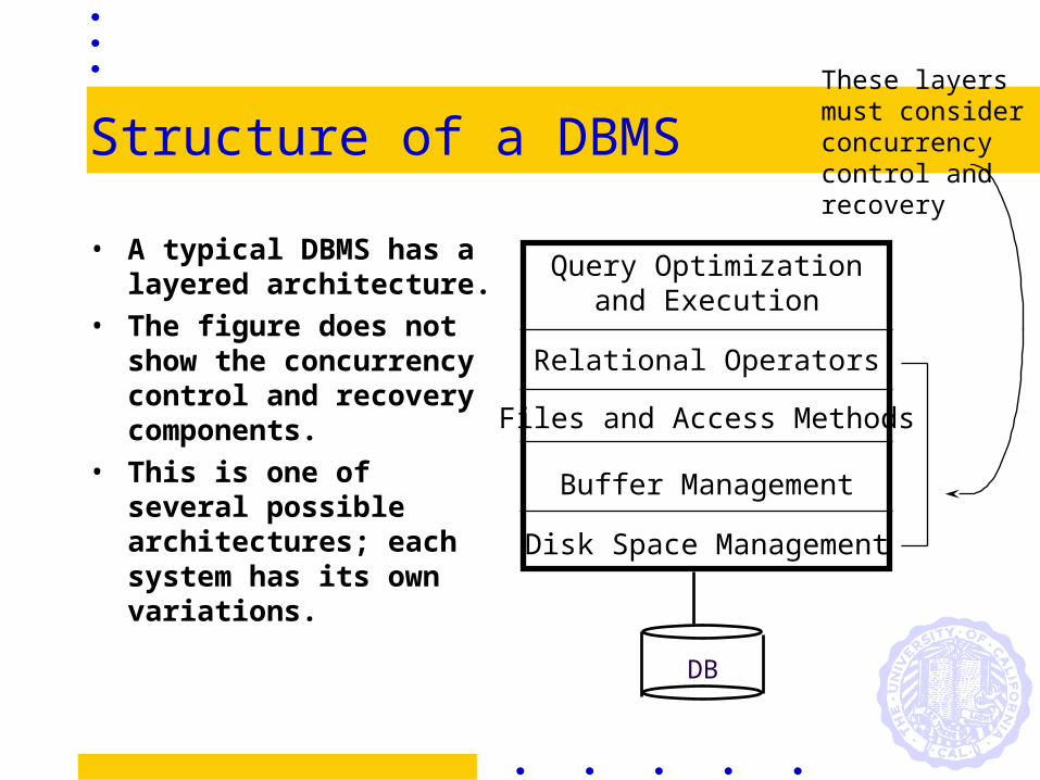
Structure of a DBMS

• A typical DBMS has a layered architecture.

• The figure does not show the concurrency control and recovery components.

• This is one of several possible architectures; each system has its own variations.

Query Optimizationand Execution

Relational Operators

Files and Access Methods

Buffer Management

Disk Space Management

DB

These layersmust considerconcurrencycontrol andrecovery

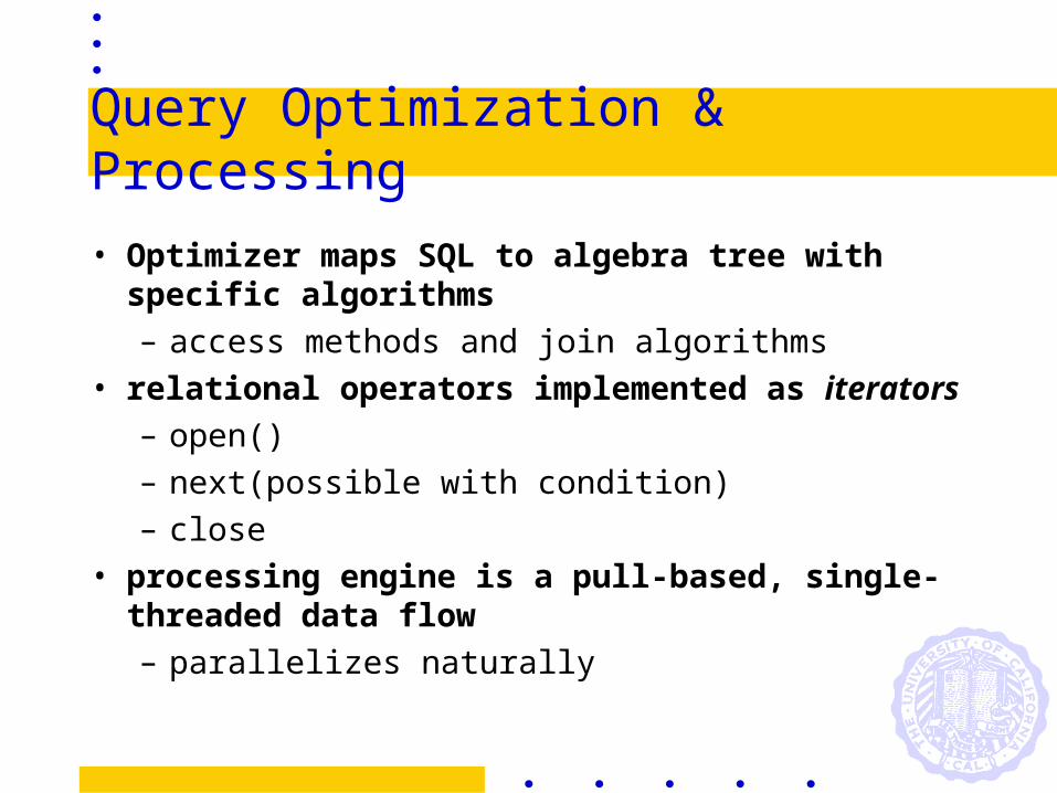
Query Optimization & Processing

• Optimizer maps SQL to algebra tree with specific algorithms– access methods and join algorithms

• relational operators implemented as iterators– open()– next(possible with condition)– close

• processing engine is a pull-based, single-threaded data flow– parallelizes naturally

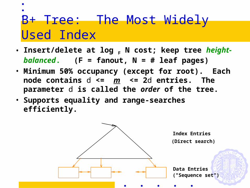
B+ Tree: The Most Widely Used Index

• Insert/delete at log F N cost; keep tree height-balanced. (F = fanout, N = # leaf pages)

• Minimum 50% occupancy (except for root). Each node contains d <= m <= 2d entries. The parameter d is called the order of the tree.

• Supports equality and range-searches efficiently.

Index Entries

Data Entries("Sequence set")

(Direct search)

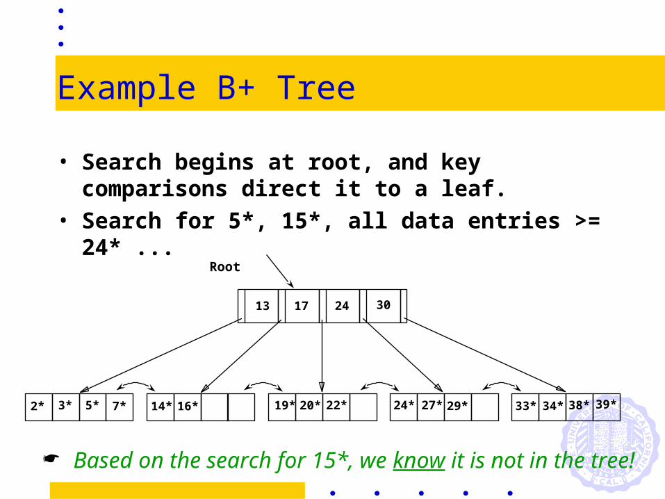
Example B+ Tree

• Search begins at root, and key comparisons direct it to a leaf.

• Search for 5*, 15*, all data entries >= 24* ...

Based on the search for 15*, we know it is not in the tree!

Root

17 24 30

2* 3* 5* 7* 14* 16* 19* 20* 22* 24* 27* 29* 33* 34* 38* 39*

13

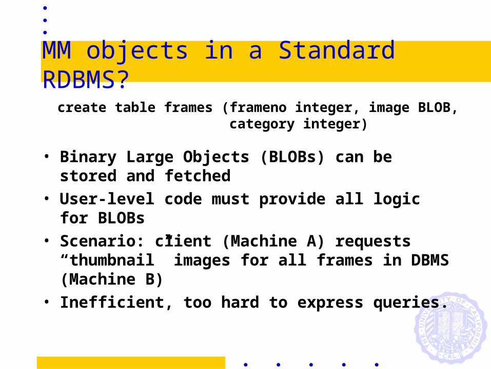
MM objects in a Standard RDBMS?

• Binary Large Objects (BLOBs) can be stored and fetched

• User-level code must provide all logic for BLOBs

• Scenario: client (Machine A) requests “thumbnail” images for all frames in DBMS (Machine B)

• Inefficient, too hard to express queries.

create table frames (frameno integer, image BLOB, category integer)

Solution 2: Object-Relational DBMS

• Idea: add OO features to the type system of SQL. I.e. “plain old SQL”, but...– columns can be of new types (ADTs)– user-defined methods on ADTs– columns can be of complex types– reference types and “deref”– inheritance and collection inheritance– old SQL schemas still work! (backwards

compatibility)• Relational vendors all moving this way (SQL99).

ADTs: User-Defined Atomic Types

• Built-in SQL types (int, float, text, etc.) limited– have simple methods as well (math, LIKE, etc.)

• ORDBMS: can define new types (& methods)create type jpeg (internallength = variable,

input = jpeg_in, output = jpeg_out);

• Not naturally composed of built-in types– new atomic types

• Need input & output methods for types– convert from text to internal type and back– we’ll see how to do method definition soon...

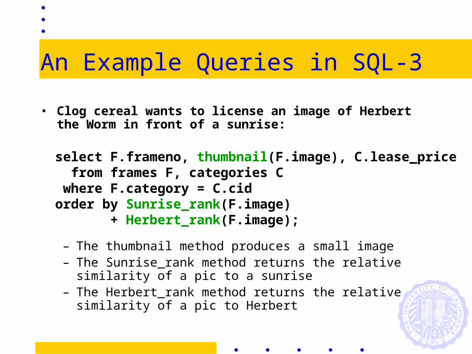
An Example Queries in SQL-3

• Clog cereal wants to license an image of Herbert the Worm in front of a sunrise:

– The thumbnail method produces a small image– The Sunrise_rank method returns the relative

similarity of a pic to a sunrise– The Herbert_rank method returns the relative

similarity of a pic to Herbert

select F.frameno, thumbnail(F.image), C.lease_price from frames F, categories C where F.category = C.cidorder by Sunrise_rank(F.image) + Herbert_rank(F.image);

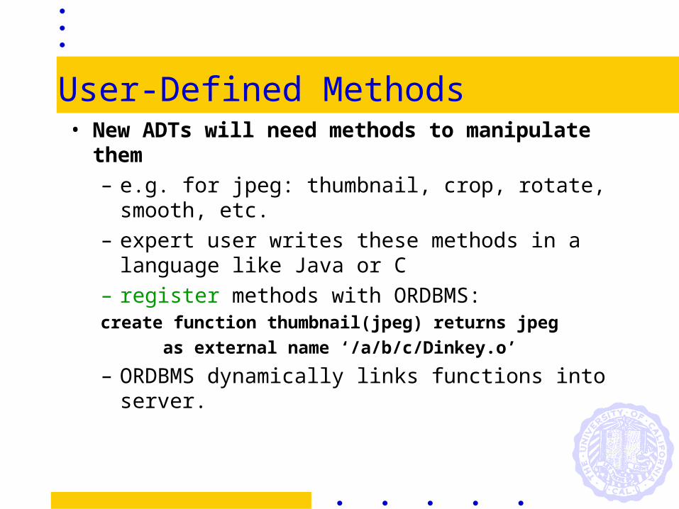
User-Defined Methods• New ADTs will need methods to manipulate

them– e.g. for jpeg: thumbnail, crop, rotate, smooth,

etc.– expert user writes these methods in a

language like Java or C– register methods with ORDBMS:create function thumbnail(jpeg) returns jpeg

as external name ‘/a/b/c/Dinkey.o’

– ORDBMS dynamically links functions into server.

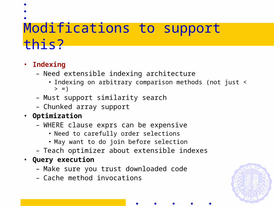
Modifications to support this?

• Indexing– Need extensible indexing architecture

• Indexing on arbitrary comparison methods (not just < > =)– Must support similarity search– Chunked array support

• Optimization– WHERE clause exprs can be expensive

• Need to carefully order selections• May want to do join before selection

– Teach optimizer about extensible indexes• Query execution

– Make sure you trust downloaded code– Cache method invocations

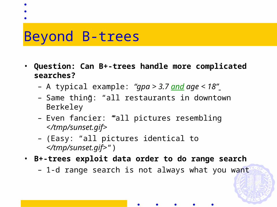
Beyond B-trees

• Question: Can B+-trees handle more complicated searches?– A typical example: “gpa > 3.7 and age < 18” – Same thing: “all restaurants in downtown Berkeley”– Even fancier: “all pictures resembling

</tmp/sunset.gif>”– (Easy: “all pictures identical to </tmp/sunset.gif>“)

• B+-trees exploit data order to do range search– 1-d range search is not always what you want

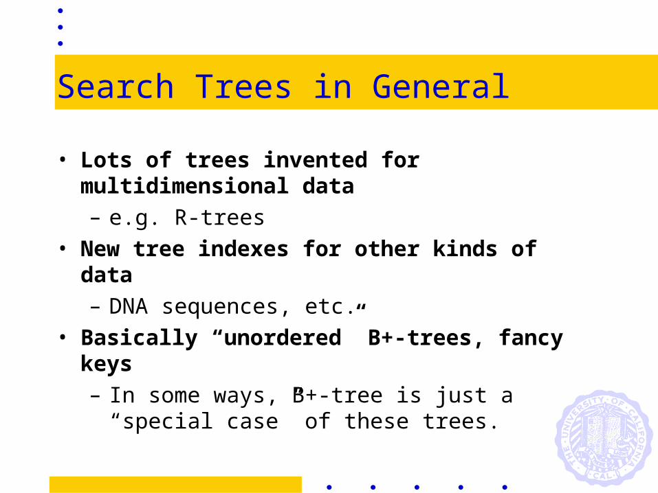
Search Trees in General

• Lots of trees invented for multidimensional data– e.g. R-trees

• New tree indexes for other kinds of data– DNA sequences, etc.

• Basically “unordered” B+-trees, fancy keys– In some ways, B+-tree is just a “special

case” of these trees.

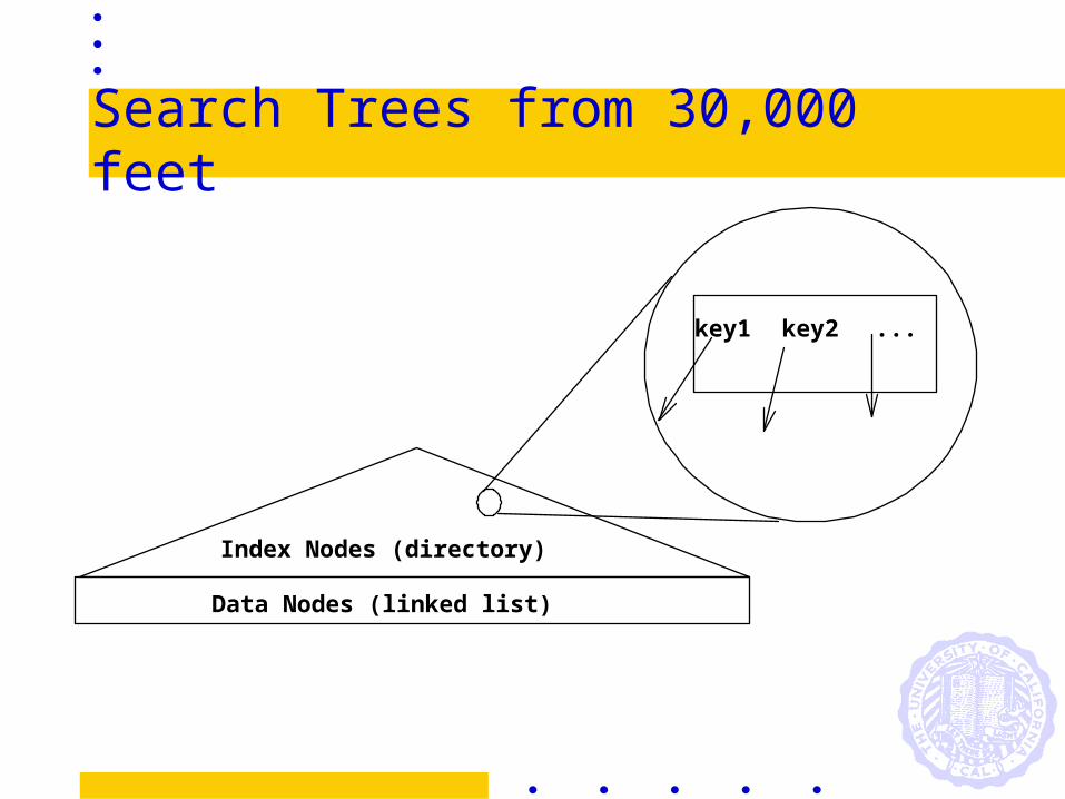
Search Trees from 30,000 feet

Index Nodes (directory)

Data Nodes (linked list)

key1 key2 ...

A “Disorderly” B+-tree

• How to search a disorderly B+-tree?– Equality search is

identical to traditional!

– Range search = traversing multiple paths

• follow all pointers where key range overlaps query range.

[32 - 61) [17 - 32) [61 - inf) [-inf - 17)

Traditional

Disorderly

17 32 61

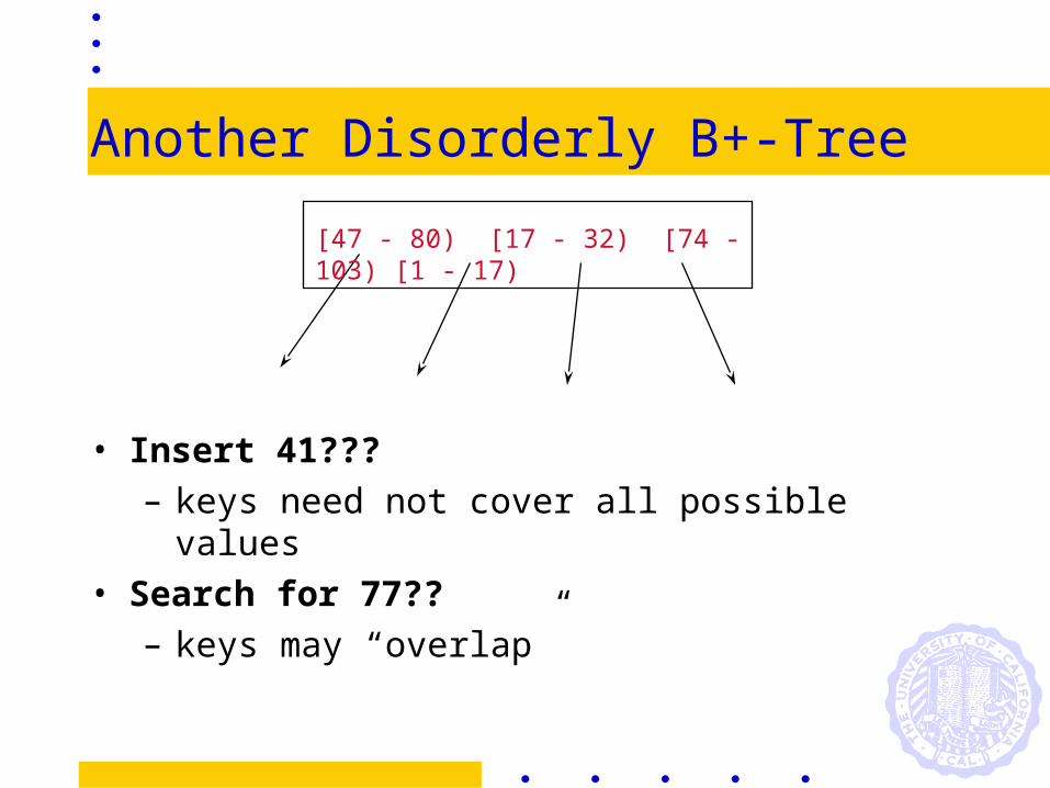
Another Disorderly B+-Tree

• Insert 41???– keys need not cover all possible values

• Search for 77??– keys may “overlap”

[47 - 80) [17 - 32) [74 - 103) [1 - 17)

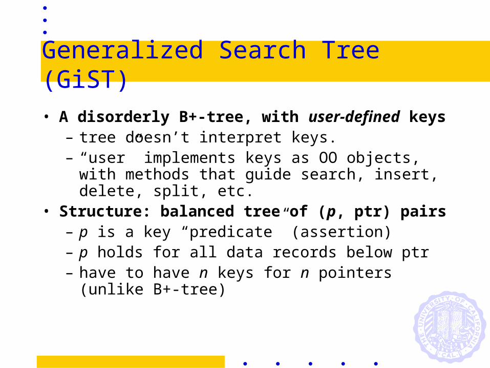
Generalized Search Tree (GiST)

• A disorderly B+-tree, with user-defined keys– tree doesn’t interpret keys.– “user” implements keys as OO objects, with

methods that guide search, insert, delete, split, etc.

• Structure: balanced tree of (p, ptr) pairs– p is a key “predicate” (assertion)– p holds for all data records below ptr– have to have n keys for n pointers (unlike

B+-tree)

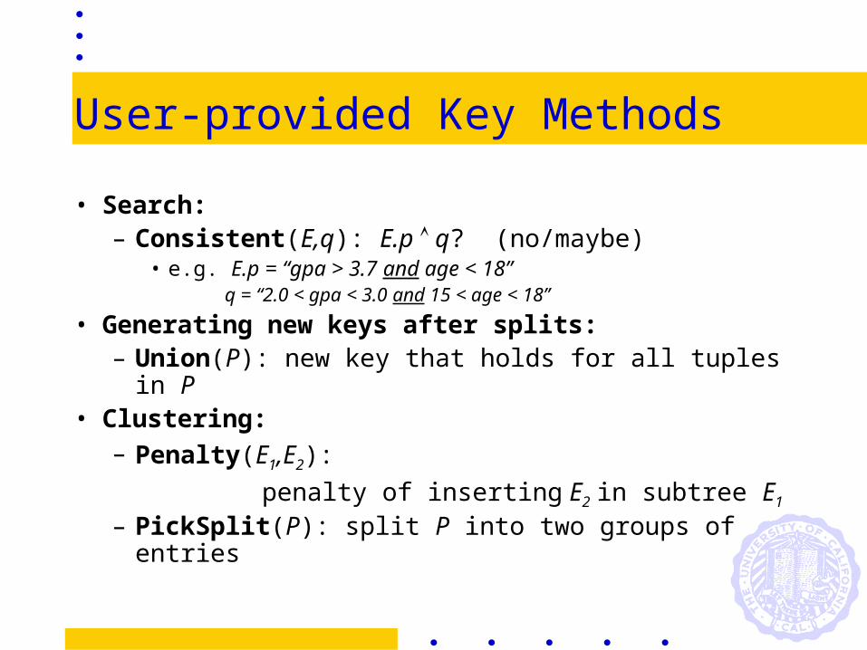
User-provided Key Methods

• Search:– Consistent(E,q): E.p q? (no/maybe)

• e.g. E.p = “gpa > 3.7 and age < 18”q = “2.0 < gpa < 3.0 and 15 < age < 18”

• Generating new keys after splits:– Union(P): new key that holds for all tuples in P

• Clustering:– Penalty(E1,E2):

penalty of inserting E2 in subtree E1

– PickSplit(P): split P into two groups of entries

Search

• General technique: – DFS tree where Consistent is TRUE

• More sophisticated– Priority queue to control the next Consistent

node to visit– Example: similarity (near-neighbor) search

for ranked queries• We’ll return to this idea

Insert

• descend tree along least increase in Penalty

• if there’s room at leaf, insert there• else split according to PickSplit• propagate changes using Union

Delete

• find the entry via Search, and delete it• propagate changes using Union• on underflow:

– reinsert stuff on page and delete page– why not borrow/merge a la B+-trees?

GiSTs over 2-d data (R-trees)

• Keys represent “minimum bounding rectangles”

• Queries: Contains, Overlaps, Equals bbox• Consistent(E,q): does E.p overlap q?• Union(P): bounding box of all entries• Penalty(E,F): size(Union({E,F})) - size(E)• PickSplit(P): different algorithms

– goal: minimize sum of areas of the 2 pages

GiSTs over sets (RD-trees)

• Logically, keys represent bounding sets• Queries: Contains, Overlaps, Equals• Consistent(E,q): does E.p q = ?• Union(P): set-union of keys• Penalty(E,F): |E.p F.p| - |E.p|• PickSplit(P): many algorithms

– goal: minimize sum of cardinalities of pages

Note: want key compression here!

An RD-tree

{CS1, CS11, Music1, Music2, Math221, Math22, Math223}

{CS1, Bus101, Bus102, Bus103, Ec121, Ec122, Ec123}

{CS1, CS786, CS888, Math221, Music1, Music788}

{Bus101, Bus102, Bus103, CS1}{Bus101, Ec121, Ec122, Ec123}

{CS1, Bus101, Ec121}

{CS1, CS11, Math221}{Music1, Music2, CS1}

{CS1, Math221, Math22, Math223}

{Music1, CS1, Math221}{Music788, CS888, CS786}

{CS1}

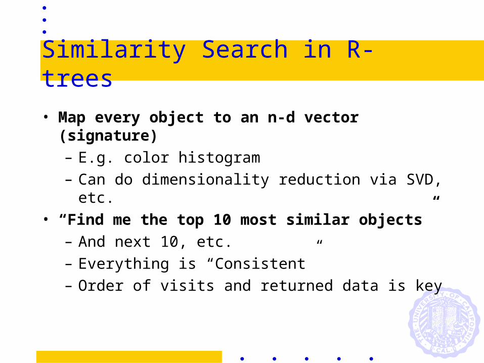
Similarity Search in R-trees

• Map every object to an n-d vector (signature)– E.g. color histogram– Can do dimensionality reduction via SVD,

etc.• “Find me the top 10 most similar

objects”– And next 10, etc.– Everything is “Consistent”– Order of visits and returned data is key

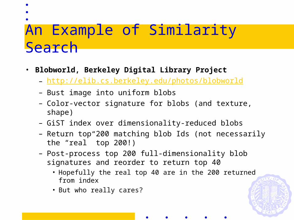
An Example of Similarity Search

• Blobworld, Berkeley Digital Library Project– http://elib.cs.berkeley.edu/photos/blobworld– Bust image into uniform blobs– Color-vector signature for blobs (and texture, shape)– GiST index over dimensionality-reduced blobs– Return top 200 matching blob Ids (not necessarily

the “real” top 200!)– Post-process top 200 full-dimensionality blob

signatures and reorder to return top 40• Hopefully the real top 40 are in the 200 returned from

index• But who really cares?

Q

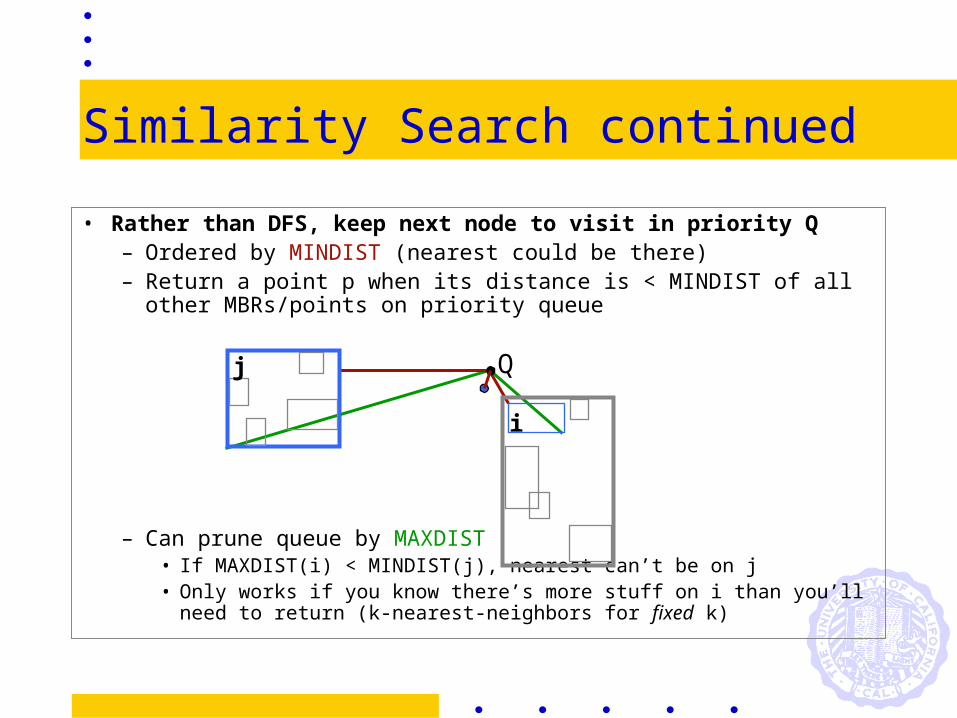
Similarity Search continued

• Rather than DFS, keep next node to visit in priority Q– Ordered by MINDIST (nearest could be there)– Return a point p when its distance is < MINDIST of all

other MBRs/points on priority queue

– Can prune queue by MAXDIST • If MAXDIST(i) < MINDIST(j), nearest can’t be on j• Only works if you know there’s more stuff on i than you’ll

need to return (k-nearest-neighbors for fixed k)

i

j

Near-Neighbor Keys

• Have been multiple proposals for other NN keys– Spheres (SS-tree), sphere/rect combo (SR-tree)

• Sphere-based Penalty gives smaller diameter clusters• Box keys reduce volume better

– Blobworld (Megan Thomas) observation:• NN-queries are like expanding circles• Circles intersect rectangles at corners• Take “bites” out of rect corners

– Aggressive Insertion• Can do insertion via NN-search, too

GiST Performance

• B+-trees have O(log n) performance• R-trees, RD-trees have no such guarantee

– search may have to traverse multiple paths– worst-case O(2n) to traverse entire tree– aggravated by random I/O: much worse

than heapfile scan!Q: when does it pay to build/use/invent an

index? Indexability theory.Q: I can’t prove there’s no good index.

How good is mine? AMDB.

Leaf-Level Statistics

I/O counts and corresponding overheads under various scenarios

{Breakdown of lossesagainst optimal clustering {

Total or per query breakdown

Global View Provides summary of node statistics for entire tree

Tree View Also displays node stats

Bounding Predicate Statistics

Views highlightnodes traversed by query

Query breakdown in terms of “empty” and required I/O.

Excess Coverage Overheads due to loose/wide BPs

Debugging Operations

Tree View Shows structural organization of index.

Highlights current traversal path during debugging steps.

Stepping Controls

Breakpoint Table Defines and enables breakpoints on events

Console window Displays search results, debugging output, and other status info.

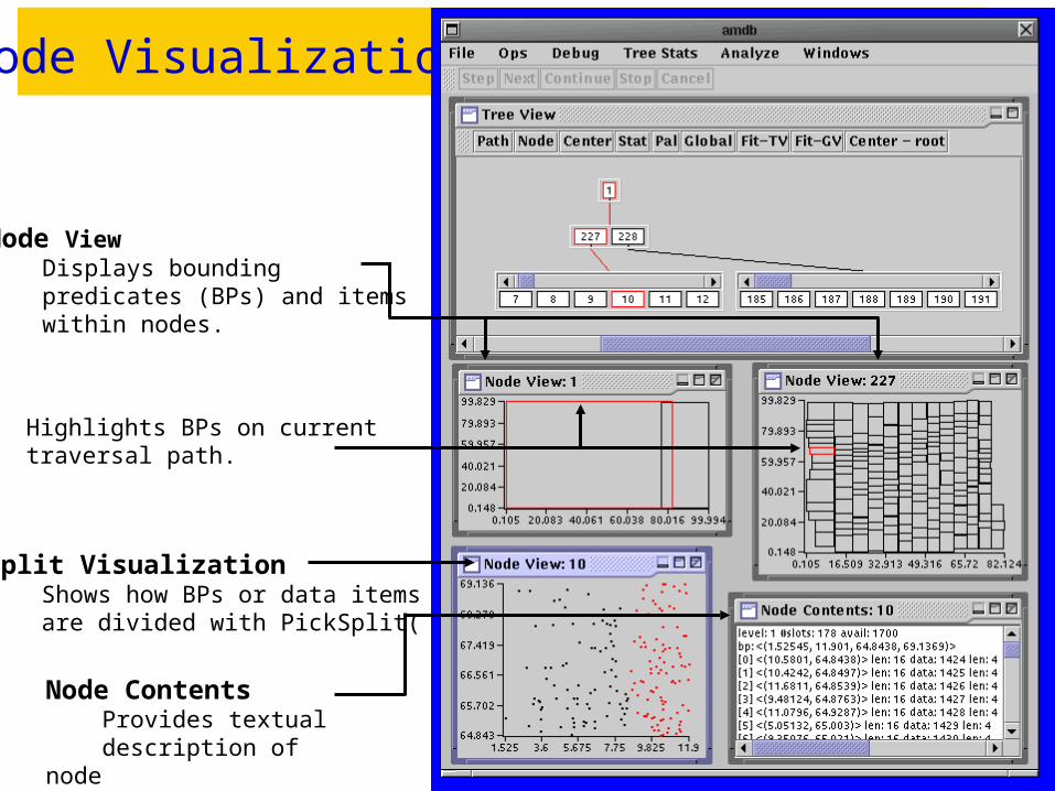
Node Visualization

Node View Displays bounding predicates (BPs) and items within nodes.

Node Contents Provides textual description of node

Split Visualization Shows how BPs or data items are divided with PickSplit( )

Highlights BPs on currenttraversal path.