For geographic applications, satellite image data must be combined withaerial photos, census data, and existing maps. Integrating the various

dataforms is a complex, multistep operation.

Pictorial Information Processing of

Landsat Data for B-IBTGeographicAnalysis L

Albert L. ZobristJet Propulsion Laboratory

Georgy NagyUniversity of Nebraska

Geographic analysis can be traced to ancient roots:the establishment of the Roman road nework, the Egyp-tian census (used for levying taxes, of course), and thelayout of the Sumerian canal system. However, not untilthe invention of the balloon in 1789 and of photographyin 1839 could large areas of the earth be pictured. TheCivil War saw the first tactical application of airbornephotography, which blossomed during the first half ofthe twentieth century into the systematic coverage of en-tire countries for cartographic purposes. The Apollo,Gemini, and Skylab flights dramatically increased thearea that could be covered in a single picture, while theintroduction in the late fifties of the multispectral scan-ner and of sideways-looking radar extended pictorialdata collection to the invisible portions of the elec-tromagnetic spectrum.

Satellite image acquisition

The systematic application of remote sensing anddigital image processing to geographic analysis beganwith the launching of the ERTS-A earth resourcessatellite, the first of the Landsat series currently in orbit.(The resolution of the Nimbus, Tyros, and ITOSmeteorological satellites was too low for most geographicpurposes.) ERTS-A, subsequently renamed Landsat 1,was preceded by five years of intense planning led byNASA. Responsibility for satellite operation and imageacquisition and distribution is gradually being trans-ferred to the National Oceanic and Atmospheric Agencyof the Department of Commerce, with NASA retainingmajor responsibility for advanced development andresearch. Currently, Landsat products may be obtained(for a fee) from the Earth Resources ObservationSystem-EROS-Data Center of the US GeologicalSurvey. Private ownership and operation of the US pro-

gram, under federal government regulation, is theultimate objective.

Landsat 3, the more recently launched of the two cur-rently operational earth resources satellites, is in a near-polar, sun-synchronous orbit-that is, it revisits eachlocation when the sun is at about the same angle-at amean altitude of 920 kilometers. It circles the earth every103 minutes, and returns to the same orbit every 18 days.With two satellites, therefore, repetitive coverage everynine days is obtainable, in principle. The position and at-titude of the satellite are tracked continuously; this track-ing data is the input for the registration procedure usedto find the approximate location of the satellite images.The location of selected scenes can then be determinedmore precisely by matching portions of the images tostored images whose locations are known.

The current Landsats have two independent image ac-quisition systems. One is provided by a four- or five-channel multispectral radiometer-MSS-and two orthree panchromatic return-beam vidicon-RBV-cameras. The multispectral scanners use an oscillatingmirror to obtain six rows of 3240 samples,.at sampling in-tervals of 9.94 milliseconds, on each mirror sweep. Themotion of the satellite produces a frame consisting of2400 scan lines. A single MSS frame represents a 185 x170-kilometer area on the surface of the earth. The inten-sity of radiation is quantized in 64 intervals, correspond-ing to one 6-bit byte. Each four-band picture thus re-quires about 30,000,000 bytes, with each one-byte pixelcorresponding to a 57 x 80-meter area. The spectral win-dows are in the 0.5 to 1.1-micrometer range, with twobands in the visible region and two in the near-infrared.The fifth channel on Landsat 3 is in the thermal-infraredregion of 10.4 to 12.6 micrometers. The spectral channelswere selected to correspond to transparent windows ofthe atmosphere, which are also useful for characterizing

0018-9162/81/1100-0034$00.75 1981 IEEE COMPUTER34

land cover types for various applications. The MSS onLandsat 3 ceased operation in 1981.The format of the Landsat 3 return-beam vidicons is

5375 x 4125 pixels. The two cameras each view a 99 x99-kilometer segment of the earth, called a subscene.Four subscences are combined to form a scene approx-imately as big as a single MSS frame. One RBV pictureelement corresponds to a 19 x 19-meter area on earth.The image information is either transmitted directly to

earth (many countries, most recently the People'sRepublic of China, are considering or already operatingground receiving stations) or, when the satellite is out ofrange of the ground receiver, stored on board onmagnetic tape for subsequent transmission. On-boardstorage has proved unreliable and will be obviated whenthe Tracking and Data Relay Satellite System is installed.Each geosynchronous TDRSS satellite will have veryhigh bandwidth (up to 300 megabits/second) trans-ponders and will relay the Landsat data to a single stationat White Sands, N.M. From White Sands, the data willbe retransmitted to Goddard via Domsat and, after pre-processing at Goddard, transmitted via Domsat to theEROS Data Center for product generation andarchiving.

Landsat image processing, archiving, anddistribution

The combined Goddard and EROS facilities for pro-cessing Landsat data must surely be the largest-or atleast the highest-volume-civilian image processingfacility in existence. During the 1980 fiscal year, for ex-ample, about 26,000 Landsat scenes were received andprocessed at the EROS Data Center. The sales volume infiscal 1980 was $2,400,000-128,000 scenes were sold inphotographic form (down from a 1976 peak of 297,000frames) and about 4100 scenes in digital form. Thefederal government accounted for 26 percent of the pur-chases, 3 percent were sold to state/local government, 25percent to industrial users, 9 percent to academic users, 4percent to individuals, and a startling 42 percent to non-US customers.The MSS and RBV images received from Landsat are

system-corrected at the NASA/Goddard Image Process-ing Facility. Radiometric correction removes sensor anddigitizer anomalies. Geometric correction is necessary tocompensate for satellite attitude changes, slewing in-troduced by satellite motion during each scan, and the ef-fects of the angle subtended by the satellite's field ofview. The characteristics of the corrected images aregiven in the Landsat Data User's Handbook.' The im-ages are resampled to a Hotine Oblique Mercator projec-tion. (Resampling means that the gray value assigned toeach point in the target image is a function-usually aweighted average-of the points corresponding to thetarget point in the source image.) The resampled MSSframes contain 3548 x 2983 pixels, while the resampledRBV subscenes contain 5322 x 5322 pixels.The standard error in the system-corrected data is

about 160 meters in each direction. Linear least-squareanalysis indicates that using linear correction factors to

remove certain errors in scale, earth rotation effect, andaspect ratio could reduce the standard error to 50 meters(less than one pixel), which would meet the National MapStandards for 1:250,000 scale. The current products arewithin the required accuracy for 1:1,000,000 scale.Haze removal, an optional process, compensates for

atmospheric scatter. Another optional process, contraststretching, allows the use of the full dynamic range of thesystem for low-contrast images. Edge enhancement,which exaggerates the difference between a given pixeland a user-specified neighborhood (kernel), is alsoavailable. Users who prefer to avoid the loss ofdiscrimination due to resampling may request onlyradiometrically corrected data; this results in some loss inpositional accuracy.

In summary, the systematic "bulk" correction of allLandsat image data takes place at the NASA/GoddardImage Processing Facility. IPF receives ephemeris datafrom the tracking stations, including postion, pitch, yaw,and altitude as a function of time. The data from thesatellite itself contains radiometric and calibration data:readings from the MSS calibration wedges, RBV calibra-tion lamp readings, and reseau marks from the RBV vidi-cons. This information is compiled with prelaunchcalibration measurements, characteristics of thetransmission channels, and cartographic constantsdescribing the geoid to allow precise reconstruction ofeach scene. Both fully corrected images and partially cor-rected images accompanied by the necessary correctionfactors are recorded on high-density (20,000-bpi)magnetic tape and transmitted to the EROS data centerin Sioux Falls.At the EROS Image Data Processing Facility the data

is archived on high-density tapes. Archival data isgenerated at a rate roughly corresponding to the outputof 200,000 keypunch operators working day and night.The image data is distributed on request in the form ofeither high-resolution (laser-recorded) photographicproducts or as standard digital computer tapes. A digitalbrowse file of selected catalog information is alsoavailable through dial-up terminals via Telenet. Specialprocessing of both film and digital data is undertaken atuser request on one of the three major image-processingcomputer systems. User training is available throughspecial workshops designed to meet particular needs.

Landsat and geographical analysis

The availability of Landsat image data has broughtabout major changes in geographical analysis. Whilepilot studies in the mid-sixties attempted to demonstratewhat can be done with image data alone, it has becomeincreasingly clear that most important applications re-quire the combination of image data with many othersources of geographical information. Some pictorial in-formation systems consider pictures as data baseelements. Yet picture content is inaccessible (althoughpreprocessing may have extracted descriptors from thecontent). Pictorial information processing that dealswith the content of images seems more appropriate formost Landsat applications.

November 1981 35

A primary advantage of Landsat coverage is the abilityto quickly obtain time-varying information about largeareas. Examples include sea ice, snow cover distributionfor predicting water availability, changes in vegetativecover, urban spread, water quality, and shoreline ero-sion. Equally important is cartographic input for de-tailed mapping of the large areas of the globe hithertomapped only at larger scales. Secondary indicators per-mit drawing conclusions about demographic factors,wildlife population, agricultural practices, and landmanagement. For all of these applications a crucial ingre-dient is the combination of satellite image data withaerial photography, census data, existing maps, small-sample data, and so on. This generally requires transfor-mation of the various forms of data into a compatibleformat and extraction of the significant items.The resolution of the satellite image is constrained not

by any inherent limitation in the instrumentation but bythe immense volume of data in even relatively small areasof the image. Because of the large amounts of data, theefficiency of the transformation and data processingalgorithms is a paramount consideration. Another re-quirement introduced by the sheer mass of the data isbuilt-in checking and verification procedures to reducethe adverse effects of noise, artifacts, and inconsistenciesof various sorts. It is simply not feasible to visually in-spect and manually correct the images on a pixel-by-pixelbasis. Geographic analysis may, in fact, be viewedprimarily as a data-reduction process; a vast amount ofdata is reduced to a few elements that can be assimilatedby human decision-makers. At the same time, there is anincreasingly wide range of applications of image process-ing technology to geographic analysis. Systems originallydesigned to do pattern recognition and image manipula-tion are being expanded to perform the full gamut ofoperations needed for data integration and spatial analy-sis. As with any new technology, there are technical,economic, and conceptual barriers to wider use.Two particular problems are worthy of a concentrated

examination here: first, the need for algorithms to enableor simplify the basic operations of geographic analysis,and second, the complexity of applications in terms ofthe sequence of operations performed. In the projectsdescribed below, we attempt to illustrate this complexityby simply listing the major steps-without much ex-planation or detail. The letter codes next to each step in-dicate that one or more of the following aspects aresignificant in that step:

* A-algorithmic problems,* C-high computational expense,* G-vector or polygon data structure,* M-manual operations,* R-raster data structure, and* T-tabular data structure.

Editing and validation steps-generally ignored below-are, of course, significant to real data handling.

Desert conservation. As part of the planning activityfor the 25-million-acre California Desert ConservationArea, the Bureau of Land Management needed a surveyof vegetation and animal forage in a form that could be

integrated with other elements of the plan. Multispectralclassification of Landsat imagery was chosen as the bestmeans of obtaining this survey, considering time andmoney constraints. The goal was to integrate digital ter-rain data, such as elevation, slope, and aspect, that havea strong effect on vegetation, with ground informationfrom maps, surveys, and photointerpretation to aid inclassification. The output was required in 10 x 1°quadrangles in Lambert Conformal Conic projectionand in tabular form, categorized by grazing allotments,land ownership, and other types of boundaries.The procedure for vegetation and forage classification

consisted of 24 major steps:

1. Obtain Landsat raw data (10 frames).2. Obtain map control points from conventional

maps (M).3. Convert the-map coordinates to Lambert Con-

formal Conic grid (G).4. Find the coordinates in the Landsat frames (G).5. Find edge-match control points for all overlap-

ping Landsat frames (A, C, R).6. Adjust edge-match control points according to a

distortion model determined by the map controlpoints (A, G).

7. Perform geometric correction and map projec-tion of the Landsat frames according to the con-trol points (A, C, R).

8. Perform brightness adjustment of the Landsatframes according to differences noted in the edge-matching control points (C, R).

9. Trim edges of the Landsat frames to remove baddata (R).

10. Mosaic the 10 frames together to obtain a single,large 7400 x 7500 image (C, R).

11. Repeat steps 7-10 for three more spectral bands ofLandsat.

12. Section Landsat mosaic into 10 quadranges (A,R, G).

13. Perform geometric correction on digital terrainfile to obtain 10 quadrangles in the same grid mapprojection (A, C, R).

14. Classify land cover by unsupervised initialclustering (1993 clusters) with supervised pooling(25 final classes) by a discipline scientist (A, C, T).

15. Test the statistics on 12 areas of 400,000 acreseach (R, G, M, T). Refine the statistics (M, T).

16. Extend the classification to the entire CaliforniaDesert Conservation Area (A, C, R).

17. Coordinate digitize various boundary files such asland ownership (G).

18. Change the digitizer coordinates to Lambert Con-formal Conic grid (G).

19. Change the boundary file from vector to rasterformat (A, C, R, G).

20. Identify the polygons determined by the boun-daries (A, C, R).

21. Perform polygon overlay of classification fileswith boundary files (A, C, R, T). This yields atable of acreages of classes per district or parcel(T).

22. Perform data management operations such as

COMPUTER36

Figure 1. California desert mosaic of 12 Landsat scenes.The image size is 7400 X 7500 for each spectral band. The Figure 2. One degree quadrangle extracted from the desertnear-infrared band is shown here. mosaic with grazing allotments superimposed.

sort, merge, merge correlate, aggregate, and The procedure for the health impact interpretationcross-tabulate on the results of polygon overlays consisted of 14 major steps:

(T). I. Find control noints in boundary files (M).23. Report the tables by printer listing or magnetic

tape (T).24. Report the image products by photographic im-

age playback or magnetic tape (R).

The results of the California Desert Task were used as aprimary input to the Desert Master Plan for range forageallocation for livestock and wild burros. The work wasperformed within a two-year deadline, primarily indigital format to facilitate 10-year updates mandated byCongress. Details of the work and utilization of theresults can be found in McLeod and Johnson2 and in theBureau of Land Management's report,3 respectively.Figure I shows the California desert mosaic with two ad-ditional Landsat frames added. Figure 2 shows a 1°quadrangle with grazing allotments superimposeddigitally. Figure 3 illustrates the tabulation of biomass bygrazing allotment.

Air pollution study. Several agencies in the Portland,Oregon, area have been working under the general coor-dination of the Pacific Northwest Regional Commissionto determine the utility of Landsat digital images for ur-ban applications. A map of land use from Landsat wasprepared at the USGS EROS Data Center, withassistance from the NASA Ames Research Center. Theapplication described here used the map to allocatepopulation from the 1973 census update to traffic zonesand two-kilometer grid cells. The grid-cell populationwas combined with air pollution data from the OregonDepartment of Environment Quality to obtain a healthimpact map.

November 1981

2. Find the same control points in the Landsat image(G).

3. Calculate a distortion surface from the controlpoints (A, G).

Figure 3. Partial tabulation of biomass for analysis of grazing capacity.

37

47054013, 3533340 N 25S3t 3430- 535Dj S

,043,54 S00~554 534304I 5140.Oo 30 S5-Ut,L03. 40044 00453e * A

I 4,4.43 0.0 45411. 43. H M..3 i'0

200 2,5240. i,40s1550.54 ? se 92, il.*@ f535

ts 522)z5 i" s5244.0044453.?-53 3433.7 34323.7 *--34v.4 io

4, 0014.303,~504. 5- \i3i034 2513.35j3 4d-s *24 ?,,s3 t'"2

50 24 .3 3445.l20 9 543.352t7 5-223544.30 3.2 i44.4-i)4

053437t44.0 0,5 t5:3375731 te-5 12.o 2,,351 tt

00 7043.0537* :3 3333t t? S 933. i5.3 3"222 ttljtS3 4443.52 3353:43? 573.3 4¢4:5j0 Jtb:'s

Jf 2552M.277 1;21,7,.74 14U744 '25 ,S

043 500s.53 s254.04 33 .,4 00.42 30S*s 35'.55jt

s34s5 0340.4ss337s-s2 402.05i 770' li3 ,,

0, 53454su.50 [53044.54s 4024j3.43 3'£303.'5 i80t 5.bs 0'' 57t03000.0.0 44430252.5 5000.35 i 13 t- *:s ,'s;itl t; ! f *o£

00 303343.543 3253444 3t 4)§x3543 0 500*9ki 597,t3., 33os 1333359.,? ''?4*o3 s°os9 lus334.03o ,-sS3: £tf3:32343332zsoU27-53 7330.53 3.0034:3; t7g-3. 's.3:3 , S:3 s:t

322r s39sl477.444 4.47 003.0s 342.3g 13 3fr&2o 2ii .tf

3s3 as,s:it 3 2-s1°0. 1>Z30I0ti v35.4 0.0:z 135.04- 1so3ss

5.45U4 3.4 3.0 313 3lt35 711544 33304 3405 345.5 a503305.54555.5 0045.03 047.55 324.34 454.4033

04 34401.30 0055 05 34 0.403 .

tt L .104533 I A I IIW~~?0*0.2.t It03.3 0. M 55

1,01 703.:7i t~~~~~~0.3 34:54441.1 ..0313.0 8055440:~t ~3.':31 'h~'031 0033.0 p5.74 3

* 0.0 ~ ~~~"I: 7jt L

Figure 4. Land use map of Portland, Oregon, derived from Landsat databy digital classification with census-tract boundaries superimposed.

PQETL6NO. OREGONPLLUITION RY G210 CELl

G21C CELL POPULATION

2,10 1163,10 147

3.113 1143. 13 11404, 9 10I4,10 13S4,11 1524.12 2944,113 11554.14 12794.17 795, 9 1325.10 1995,11 1635,12 1185.13 7665.14 8275,15 479

35.14 97436. 1 8253S.12 599

915092

POLL VALUE

2829322829292929292928292828i2 d

P0(1 10NEX COVERAGE

3236 92

33 33 10031911 91

2912 1003929 1004397 1008513 10033490 10037098 9622033832598^

31 347083 i 634 7III530 2922730 2475130 17982

361014490

10098

100100100913100100

Figure 5. Partial tabulation of health effect of air pollution of two-kilo-meter grid cell. This is a function of population and air pollution.

4. Geometrically correct the boundary files accord-ing to the distortion surface (G).

5. Change the boundary file from vector to rasterformat (A, C, R, G).

6. Identify the polygons determined by the boun-daries (A, C, R).

7. Perform polygon overlay of classification fileswith boundary files (A, C, R, T). This yields atable of acreage of classes per zone or cell (T).

8. Rearrange the table of acreages and produce aprinted report (T).

9. Perform polygon overlay of the census tracts withthe grid cells taking the sum of residential pixels ineach intersection (A, C, R, T).

10. Merge the population data according to censustract keys (T).

11. Disaggregate the population data over the tract-cell intersections in proportion to the sum ofresidential pixels (T).

12. Reaggregate the population data by grid cell (T).13. Multiply population per grid cell by pollution per

grid cell to obtain a tabulation of health effectand produce a printed report (T).

14. Inject the health-effect tabular values into thegrid-cell image to give a choroplethic map ofhealth effect (R, T).

The Portland agencies can now combine these resultswith new data sets produced from the grid pollutionmodel to calculate health effect on 1973 population. It isalso easy to use census updates or projections to obtainhealth effects at a desired date. Parenthetically, censusupdates and projections are rather hard to do, but areundertaken by the Bureau of the Census and other agen-cies. Details are given in Bryant et al.4 Figure 4 shows theland use map derived from Landsat with political boun-daries overlaid. Figure 5 is a partial tabulation of healtheffect by grid cell. Figure 6 is the map of health effect bygrid cell.

Figure 6. Choroplethic map of health effect by grid cell generated fromthe tabulation.

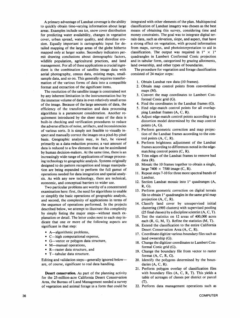
Urban expansion delineation. The Geography Divisionof the US Bureau of the Census was interested in the ur-

ban growth of the Orlando, Florida, region during1970-1975. Since Landsat I was not placed into orbit un-

til 1972, this study had to compare a 1975 land cover map

derived from Landsat to a 1970 base constructed fromthe decennial census.

The procedure for assessing urban expansion consistedof 16 major steps:

1-6. Same as Portland case (above).7. Count the pixels in each polygon to produce a

table of areas (R, T).8. Merge the census population data into the table

of areas according to census track keys (T).9. Divide population by area and use 1000 people

per square mile as a threshold for urban/non-urban (T).

10. Inject the urban/non-urban values into the cen-

sus track image to give a choroplethic map (R,T).11. Use classification to extract basic land cover

from the 1975 Landsat (A, C, R, G, T, M).12. Use an image cell-value translation routine to

COMPU1 ER

PORTLAND, OREGON IAIR POLLUTION

PELATIVE HEALTH IMPAoCT1973 POP. X POLL.

IC~~~~~ C15S -_

3 E3 033- aoU

1- l5

I~~~~~~~~~4.S fo o:I: 8iS.o:

U *

V..~~~ ~ ~ ~~~~~L5.CU G

38

convert the classes to urban/non-urban (R).13. Use polygon overlay to produce tables of

urban/non-urban land use by census tract (A, C,R, T).

14. Merge the tables according to census-tract key toproduce a single table comparing urban growthby census tract for 1970-1975 (T).

15. Digitally overlay the census tract boundaries onthe two urban area images to produce maps (R).

16. Use an image arithmetic combination routine toproduce a change map (A, R).

It is interesting to note that Landsat data forms anhistorical archive over large areas of the earth datingback to 1972. Here, the status of an area in 1975 wasretrieved. For a report, see Friedman and Angelici.5Figure 7 shoiws the map of urban change, 1970-1975.

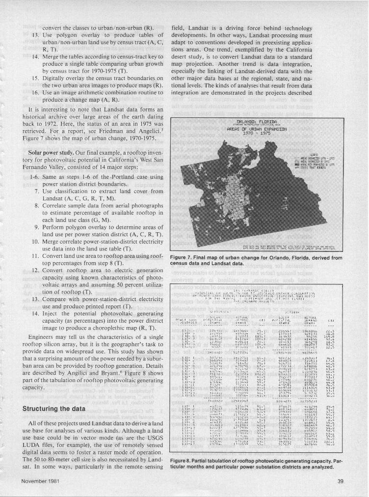
Solar power study. Our final example, a rooftop inven-tory for photovoltaic potential in California's West SanFernando Valley, consisted of 14 major steps:

1-6. Same as steps 1-6 of the Portland case usingpower station district boundaries.

7. Use classification to extract land cover fromLandsat (A, C, G, R, T, M).

8. Correlate sample data from aerial photographsto estimate percentage of available rooftop ineach land use class (G, M).

9. Perform polygon overlay to determine areas ofland use per power station district (A, C, R, T).

10. Merge correlate power-station-district electricityuse data into the land use table (T).

11. Convert land use area to rooftop area using roof-top percentages from step 8 (T).

12. Convert rooftop area to electric generationcapacity using known characteristics of photo-voltaic arrays and assuming 50 percent utiliza-tion of rooftop (T).

13. Compare with power-station-district electricityuse and produce printed report (T).

14. Inject the potential photovoltaic generatingcapacity (as percentages) into the power districtimage to produce a choroplethic map (R, T).

Engineers may tell us the characteristics of a singlerooftop silicon array, but it is the geographer's task toprovide data on widespread use. This study has shownthat a surprising amount of the power needed by a subur-ban area can be provided by rooftop generation. Detailsare described by Angilici and Bryant.6 Figure 8 showspart of the tabulation of rooftop photovoltaic generatingcapacity.

Structuring the data

All of these projects used Landsat data to derive a landuse base for analyses of various kinds. Although a landuse base could be in vector mode (as are the USGSLUDA files, for example), the use of remotely senseddigital data seems to foster a raster mode of operation.The 50 to 80-meter cell size is also necessitated by Land-sat. In some ways, particularly in the remote sensing

field, Landsat is a driving force behind technologydevelopments. In other ways, Landsat processing mustadapt to conventions developed in preexisting applica-tions areas. One trend, exemplified by the Californiadesert study, is to convert Landsat data to a standardmap projection. Another trend is data integration,especially the linking of Landsat-derived data with theother major data bases at the regional, state, and na-tional levels. The kinds of analyses that result from dataintegration are demonstrated in the projects described

Figure 7. Final map of urban change for Orlando, Florida, derived fromcensus data and Landsat data.

Figure 8. Partial tabulation of rooftop photovoltaic generating capacity. Par-ticular months and particular power substation districts are analyzed.

November 1981

ORLADO, FLOR:DAR -S 9 -

AREAS L URSMDAt PAISIO

S7O ;- I975

^ - ,Z31I, M5Tj,0 ' 575

_S=~~I - - 1X -_ s _~~~~~~~~~~13 _83008S ~~~ ~ ~ ~ ~ ~ ~ ~~__5E 063i010

90 ,-,NAr340 ;ALL -P,AIL,',A IA KL'LI 3-1SF3328 3)93 3k6t7rF, (ryCLNSUMPT? (

f11FIKis INT,3S (,, PTE.HEF ANLL 'Cl_

1PST 19i 68PIIlI INAPY 3-SOILTS

TLk 33J3L SOL ALTUALUliltICII tZh | 4 t~~~~~~~~~~~~,""tI (KW WTIt..l-3 '.033-P7T,3.716) 3'-3ONjO ~~~~~~~II3307,T AL DE81AND A

133--, 274);, ~~I,J,10f44, ON5 236447 1064046 2.t,,,- ; 279 .4, '.39,,'. NO.2 140 g 7N ' 2r 14 73 0 6.1 iO- h 189s)2, 102373 1US.3 16347 96256 165.8113- 1 4D,907 4412o 1o0i.3 4J4201 414647 97.413 I 2 `,h01I, 20.1 10,1 4) 364258 18.51 t 63ss7r 10 .1 6.,619 660787 97.6I1, 3,3311 11.I 413d) 331917 12.S

3--,2 5J713N1 2941939 4'35465I1 1- I sd 33Sh 1 1 7s, N . 5301 r32 1,i07 36.1AAl- '.566393 71e497 re.3 48,1)24 721513 C7.6iIL 5 dd7 7

0127 . 502713 4787 64.6131- 4 3 I1 7'. ,7 .241 41. 277234 678006 '.0.I31 .l- .! 4 92 142 74. 370'`5 624759 s3.dI11 .C' 3-.28 '.N 4,.47-7 1334030 40.531L 7 741 6,3 12 r177 102.) 6 2,31 723199 rr.,Iil- r 11 7,59 0 b6.9 39222 7391U37 53.1I11- 322111, 6,7394 4'6.9 277542 690276 40.2

t, 4t- 1i2972341

3 9d 6l59 I

s 359 47r

1110 514 2349 9. 371921 833519 44.

131-1 671io002513 '..I Ie87T7 116314 43.8I11l-l 7 2 1 09,0 5-.' b65969 12331323 3.1I 1-I,. 413,,, -!99 4. 38 457 2 35.41I1-191l'.-I 31 3,I O.4 41.9 143 1 / 3992 33 36.0

1933,320 12039J47 633,J91 1.167231133--1 71u. 953079 81.9 316625 42L294 39.41 33-3 ,702 97 74'. 569.3 41343 6001 71.2133- 3211r 91'-o1 52.4 279334 406368 57.4133- -6/.67, 117602I 94. 4994) 901187 59).7

1t3- 9 241 7, 1041

5 d. 4 613 2 4 7 6 71231.+.l J 60 IJi9 34.377brD b51? 65.7

1 131 6-2.5 )Iw*,1 S O /25 I

6V P7 b541,4- 8 l,247 33739i3 07 36C0315l 696817 599.113 - 9 3341*3Z 198 42.s 3 192 7 646469 46 .7133-L 622 .78 123299'. 9 51.7616 392994 94.01)3-1I 4-I, J,34I3 335.6 3,6370j 3541 98.9

1303-, 0 '29 36363 79..13-1-.7 5' 73'.. ,. 391 N7, 9.0

133-173(78,, 3-30599 93. 9191250,164690.0~~~~~~~~~~~~~~~~~~~~~~~~~~9 5515?564

39

above. All four of the projects use the polygon overlayoperation to yield tabulations of spatial data. Perhapsthe most interesting of these cases was the use of Landsatdata to allocate population in Portland when everyoneknows a satellite cannot count people.The previous section has given a taste of the richness of

data structures (R, G, and T codes) and prevalence ofalgorithmic problems (A and C codes). What can be saidabout the impact of research in mathematics, imageprocessing, and computational geometry on the develop-ment of remote sensing information systems? Withregard to data structures, the constraints have been theunderlying structure of the great data bases (Landsat,Census, etc.) and the pressure to get applications com-pleted on schedule. The former has prohibited unifica-tion of data structures (for example, conversion of alldata types to vectors). The latter has prohibited adoptionof complex data structures (quad trees, strip trees, LCFtrees, etc.) because excessive programming, data editing,and data conversion costs would be required.Two basic characteristics of geographic data structures

should be explained here. The first is the concept ofspatial registration. This can be achieved either by co-location, where predictable elements of the data struc-ture correspond to the same point on the ground, or bymapping, where a formula relates the data structureelements to a geographic coordinate system. The secondis the dual file structure. Geographic files have a spatialpart which contains points, lines, or areas, together withidentifiers. A separate file contains additional non-spatial information also keyed by identifier. An exampleis the Census DIME file.

Research on geometric algorithms has been a source ofinspiration for geographic information systems, but amajor limiting factor has been the need to retain conven-tional data structures, as outlined in the previousparagraph. Three related problems are of major concern.

First, most of the theoretical work has aimed at accept-able worst-case performance, whereas good expectedperformance or even the development of unpredictableheuristic methods would seem appropriate for economicreasons. McLemore and Zobrist' describe a heuristic forcoloring a map in four colors with no two adjacentregions the same color, with a worst case of O(n2) (if itfails to work, then it also reports that in O(n2) time).Manacher and Zobrist8 describe a method for tri-angulating a point set in shortest-edge-first fashionwhich has a worst case of O(n3) but which uses a tech-nique that obtains O(n2) average case behavior (proof notpublished).A second problem arises when algorithms are based on

complex data structures that impose unrealistic con-straints on data capture or editing. For example, manydata bases have files of polygons which are intended topartition an area but actually overlap or underlap eachother. This topological imperfection rules out manyalgorithms for polygon processing.The third problem is numerical accuracy (quantization

effects) in performance of elementary steps of analgorithm. An example is the oft-advocated method fordetermining whether a point is inside a polygon: drop aperpendicular from the point and count crossings of the

polygon boundary. An odd count implies that the pointis inside. The problem is that the perpendicular may betangent or end-intersecting to an edge in the polygon,thereby producing an error. Furthermore, this problem isspatially ill-conditioned because the regions of error canbe arbitrarily far from the polygon boundary.

Based on present successes and expected advances inremote sensing from space and in communication, datastorage, and data processing technologies, the next 30years hold an exciting promise: no less than a completeinventory of the world's major resources. Assessment offood and fiber crops, forage biomass, forests, wetlands,coastline, urban development, growth of deserts, waterresources, minerals, soils, oceans, weather, and climatewill all be affected by this vast enterprise. The inventoryprocess will not be a simple operation of pixel countingfrom remotely sensed data. Instead, the methods andmodels in present use by discipline scientists will beenhanced by the incorporation of remotely sensed datasets and rendered more efficient by the computerizedtechniques of geographic analysis now beingdeveloped. U

Acknowledgments

This article presents the results of one phase of researchcarried out at the Jet Propulsion Laboratory, CaliforniaInstitute of Technology, under contract No. NAS 7-100,sponsored by the National Aeronautics and Space Ad-ministration, and at the University of Nebraska with thesupport of the Conservation and Survey Division throughNASA grant 28-004-020.

References

1. Landsat Data User's Handbook, revised edition, USGeological Survey, Arlington, Va., 1979.

2. R. G. McLeod and H. B. Johnson, "Resource InventoryTechniques Used in the California Desert ConservationArea," presented at the Arid Lands Resource InventoryWorkshop, La Paz, Mexico, Nov. 30-Dec. 6, 1980.

3. The California Desert Conservation Area Final Environ-mental Impact Statement and Plan, US Department of In-terior, Bureau of Land Management, Oct. 1, 1980.

4. N. A. Bryant, A. J. George, Jr., and R. Hegdahl, "TabularData Base Construction and Analysis from ThematicClassified Landsat Imagery of Portland, Oregon," Proc.,Fourth Annual Symposium on Machine Processing ofRemotely Sensed Data, Laboratory for Applications ofRemote Sensing, Purdue University, West Lafayette, In-diana, June 21-23, 1977, pp. 313-318.

COMPUTER40

5. S. Z. Friedman and G. L. Angelici, "The Detection of Ur-ban Expansion from Landsat Imagery," Remote SensingQuarterly, Vol. 1, No. 1, Jan. 1979. Originally presented atspring meeting of Association of American Geographers,New Orleans, Apr. 1978.

6. G. L. Angelici and N. A. Bryant, "Solar Potential Inven-tory and Modelling," Data Resources and Requirements:Federal and Local Perspectives, contributed papers fromthe 16th Annual Conference of the Urban and Regional In-formation Systems Association, Washington, DC, Aug.6-10, 1978, pp. 442-453.

7. B. D. McLemore and A. L. Zobrist, "A Five ColorAlgorithm for Planar Maps," presented at the SecondCaribbean Conference on Combinatorics and Computing,University of the West Indies, Cave Hill, Barbados, Jan.1977.

8. G. K. Manacher and A. L. Zobrist, "Fast Average CaseGreedy Triangulation of a Planar Point Set," Proc. 16thAnnual Allerton Conference on Communication, Control,and Computing, Monticello, Ill., Oct. 4-6, 1978.

Albert L. Zobrist is presently a member ofthe technical staff at the Jet PropulsionLaboratory. He was an associate pro-fessor of computer sciences at the Univer-sity of Arizona, Tucson, 1974-75, andfrom 1970-74 was a professor of electricalengineering and computer science at theUniversity of Southern California, Los

-~ t;Angeles, where he was also a member ofAL9 1 the research staff of the Information

Sciences Institute from 1973-74. Before that, he was a memberof the technical staff at the Aerospace Corporation, El Segun-do, California.

Zobrist received the BS degree in mathematics fromMassachusetts Institute of Technology, Cambridge, in 1964,and the MS degree in mathematics and the PhD degree in com-puter science, both from the University of Wisconsin, Madison,in 1966 and 1970.

George Nagy was appointed chairman ofthe Computer Science Department of theUniversity of Nebraska in 1972 andteaches courses on computer organization,pattern recognition, and remote sensing.Prior to joining the University ofNebraska, Nagy spent 10 years on the staffof the IBM T. J. Watson Research Center,

r- developing pattern classification tech-> .Xmniques for optical character recognition,

speech processing, data compression, and remote sensing. Hiscurrent research areas are geographic data processing, digitalimage registration, and the quantitative evaluation of thehuman-computer interface.Nagy has served as a research consultant for IBM, Bell

Telephone Laboratories, Tektronix, Compression Labora-tories, and NASA. He has given lectures at over 100 universitiesand professional conferences in the United States and abroadand is the author of numerous research and survey articles. Amember of the IEEE and ACM, Nagy received the PhD degreein electrical engineering from Cornell University in 1962.

November 1981