data$mining$mtat.03.183$ … · • this slide deck is a “mashup” of the ... – marlon dumas,...
TRANSCRIPT

Data Mining MTAT.03.183
Online Analy4cal Processing and Data Warehouses
Jaak Vilo 2014 Spring

Main contents of today:
• Data Warehouse (and Business Intelligence)
• Data Cube abstracEon (Pivot Table, OLAP)
• MulE-‐dimensional modeling (Star, Snowflake)
• Advanced: Complex and evolving dimensions…
Jaak Vilo and other authors UT: Data Mining 2009 2

Acknowledgment • This slide deck is a “mashup” of the
following publicly available slide decks: – http://www.postech.ac.kr/~swhwang/grass/DataCube.ppt – http://classweb.gmu.edu/kersch/inft864/Readings/Shoshani/
DataCube/CubeNotesKerschberg.ppt – http://ohr.gsfc.nasa.gov/wfstatistics/Data_Cube_Training.ppt – http://www.cs.uiuc.edu/homes/hanj/bk2/03.ppt – Hector Garcia-Molina, Stanford University – Marlon Dumas, Univ. of Tartu, – Sulev Reisberg, Quretec & STACC – Torben Bach Pedersen , Aalborg University, DK
– …
Aalborg University 2012 - DataInt! 4!
What is Business Intelligence (BI)?"
• From Encyclopedia of Database Systems:“[BI] refers to a set of tools and techniques that enable a company to transform its business data into timely and accurate information for the decisional process, to be made available to the
right persons in the most suitable form.”"

What is Business Intelligence (BI)?"• BI is different from Artificial Intelligence (AI) ""
n AI systems make decisions for the users"n BI systems help the users make the right decisions, based on
available data "
• Combination of technologies"n Data Warehousing (DW)"n On-Line Analytical Processing (OLAP)"n Data Mining (DM)"n ……"
Aalborg University 2012 - DataInt! 5!

Aalborg University 2012 - DataInt! 6!
Case Study of an Enterprise"• Example of a chain (e.g., fashion stores or car dealers)"
n Each store maintains its own customer records and sales records"◆ Hard to answer questions like: “find the total sales of Product X from
stores in Aalborg”"n The same customer may be viewed as different customers for
different stores; hard to detect duplicate customer information"n Imprecise or missing data in the addresses of some customers"n Purchase records maintained in the operational system for limited
time (e.g., 6 months); then they are deleted or archived"n The same “product” may have different prices, or different discounts
in different stores""
• Can you see the problems of using those data for business analysis?"

Aalborg University 2012 - DataInt! 7!
Data Analysis Problems"
• The same data found in many different systems"n Example: customer data across different stores and
departments"n The same concept is defined differently"
• Heterogeneous sources"n Relational DBMS, On-Line Transaction Processing (OLTP)"n Unstructured data in files (e.g., MS Word)"n Legacy systems"n …"

Aalborg University 2012 - DataInt! 8!
Data Analysis Problems (cont’)"
• Data is suited for operational systems"n Accounting, billing, etc."n Does not support analysis across business functions"
• Data quality is bad"n Missing data, imprecise data, different use of systems"
• Data is “volatile”"n Data deleted in operational systems (6 months)"n Data changes over time – no historical information"
Data Analysis Problems (cont’)"• Kimball & Ross point out typical issues:"
n “We have mountains of data, but we can’t access it”"n “We need to slice and dice the data in every which way”"n “Make it easy to get the data directly”"n “Show me what is important”"n “Two people present the business metrics, but with different
numbers”"
• It is time for a change …"
Aalborg University 2012 - DataInt! 9!

Aalborg University 2012 - DataInt! 10!
Data Warehousing"• Solution: new analysis environment (DW) where the data is"
n Subject oriented (versus function oriented)"n Integrated (logically and physically)"n Time variant (data can always be related to time) "n Stable (data not deleted, several versions)"n Supporting management decisions (different organization)"
• Data from the operational systems is n Extracted"n Cleansed"n Transformed"n Aggregated (?)"n Loaded into the DW"
• A good DW is a prerequisite for successful BI "

Aalborg University 2012 - DataInt! 11!

Aalborg University 2012 - DataInt! 12!
DW: Purpose and Definition"
• A DW is a store of information organized in a unified data model"
• Data collected from a number of different sources"n Finance, billing, website logs, personnel, … "
• Purpose of a data warehouse (DW):"support decision making"
• Easy to perform advanced analysis"n Ad-hoc analysis and reports"
◆ We will cover this soon ……"n Data mining: discovery of hidden patterns and trends"

Aalborg University 2012 - DataInt! 13!
DW Architecture – Data as Materialized Views!
DB!
DB!
DB!
DB!
DB! Appl.!
Appl.!
Appl.!
Trans.! DW!
DM!
DM!
DM!
OLAP!
Visua-!lization!
Appl.!
Appl.!
Data !mining!
(Local) !Data Marts !
(Global) Data!Warehouse!
Existing databases!and systems (OLTP)! New databases!
and systems (OLAP)!
Analogy: (data) producers ↔ warehouse ↔ (data) consumers!

Aalborg University 2012 - DataInt! 14!
Function vs. Subject Orientation"
DB!
DB!
DB!
DB!
DB! Appl.!
Appl.!
Appl.!
Trans.! DW!
DM!
DM!
DM!
D-Appl.!
D-Appl.!
Appl.!
Appl.!
D-Appl.!
Function-oriented!systems!
Selected !subjects!
All subjects,!integrated!
Subject-oriented!systems!
Sales!
Costs!
Profit!

Aalborg University 2012 - DataInt! 15!
Hard/Infeasible Queries for OLTP"• Why not use the existing databases (OLTP) for business analysis?!• Business analysis queries!
n In the past five years, which 10 products are most profitable?!
n Which public holiday has the largest sales? !n Which week has the largest sales?!n Does the sales of dairy products increase over time?!
• Difficult to express these queries in SQL !n 3rd query: we may extract the “week” value using a
function!◆ But the user has to learn many transformation functions …!
n 4th query: use a “special” table to store IDs of all dairy products, in advance!
◆ There can be many different dairy products; there can be many other product types as well …!
• There is a need for multidimensional modeling …!

16
OLTP vs. OLAP
• OLTP – Online Transaction Processing – Traditional database technology – Many small transactions
(point queries: UPDATE or INSERT) – Avoid redundancy, normalize schemas – Access to consistent, up-to-date database
• OLTP Examples: – Flight reservation – Banking and financial transactions – Order Management, Procurement, ...
• Extremely fast response times...
Carsten Binnig, ETH Zürich

17
OLTP vs. OLAP
• OLAP – Online Analytical Processing – Big aggerate queries, no Updates – Redundancy a necessity (Materialized Views, special-
purpose indexes, de-normalized schemas) – Periodic refresh of data (daily or weekly)
• OLAP Examples – Decision support (sales per employee) – Marketing (purchases per customer) – Biomedical databases
• Goal: Response Time of seconds / few minutes
Carsten Binnig, ETH Zürich

18
OLTP vs. OLAP (Water and Oil)
• Lock Conflicts: OLAP blocks OLTP • Database design:
– OLTP normalized, OLAP de-normalized • Tuning, Optimization
– OLTP: inter-query parallelism, heuristic optimization – OLAP: intra-query parallelism, full-fledged optimization
• Freshness of Data: – OLTP: serializability – OLAP: reproducibility
• Integrity: – OLTP: ACID – OLAP: Sampling, Confidence Intervals
Carsten Binnig, ETH Zürich
Atomicity Consistency Isolation Durability
19
Solution: Data Warehouse
• Special Sandbox for OLAP • Data input using OLTP systems • Data Warehouse aggregates and replicates data
(special schema) • New Data is periodically uploaded to Warehouse
Carsten Binnig, ETH Zürich
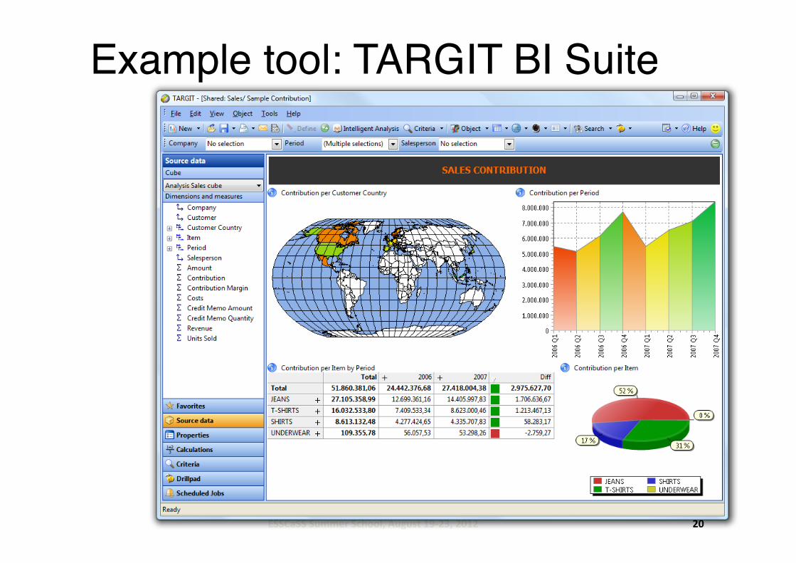
Example tool: TARGIT BI Suite"
ESSCaSS Summer School, August 19-‐23, 2012 20

2. Data Cube abstracEon
• Pivot Table
• The “data cube” abstraction
• Multidimensional data models

Sales data example
ID Region Store Category product date sale1 Tallinn Ylemiste TV Samsung 13.10.2011 10002 Tartu Lõunakeskus TV Samsung 12.10.2011 9803 Tallinn Mustika Radio Sony 10.9.2011 12004 Tartu Lõunakeskus Radio Sony 11.11.2011 11505 Tallinn Ylemiste TV Samsung 11.11.2011 9906 Tartu Lõunakeskus TV Philips 12.11.2011 15007 Rakvere Lõunakeskus TV Samsung 13.9.2010 3008 Tartu Lõunakeskus TV Sony 12.9.2011 12009 Tallinn Mustika Radio Philips 11.11.2011 35010 Tartu Lõunakeskus TV Sony 11.11.2011 1150
Jaak Vilo and other authors UT: Data Mining 2009 22

Excel pivot table
Column'LabelsCount'of'ID Sum'of'sale Total'Count'of'ID Total'Sum'of'sale
Row'Labels Radio TV Radio TVRakvere 1 300 1 300Tallinn 2 2 1550 1990 4 3540Tartu 1 4 1150 4830 5 5980Grand&Total 3 7 2700 7120 10 9820
Jaak Vilo and other authors UT: Data Mining 2009 23
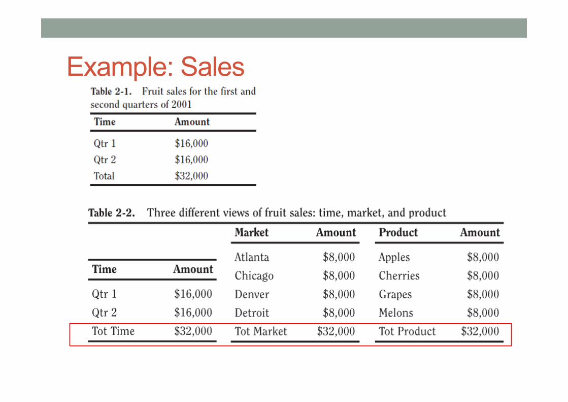
Example: Sales

Multidimensional View of Sales • Multidimensional analysis involves viewing data simultaneously
categorized along potentially many dimensions

Pivoting


Typical Data Analysis Process
• Formulate a query to extract relevant information • Extract aggregated data from the database • Visualize the result to look for patterns. • Analyze the result and formulate new queries. • Online Analytical Processing (OLAP) is about
supporting such processes • OLAP characteristics: No updates, lots of
aggregation, need to visualize and to interact • Let’s first talk about aggregation…

Relational Aggregation Operators • SQL has several aggregate operators:
– SUM(), MIN(), MAX(), COUNT(), AVG() • The basic idea is:
– Combine all values in a column into a single scalar value
• Syntax – SELECT AVG(Temp) FROM Weather;
IDSLab.
5 17 2
. . .
13
? …
AVG()

The Relational GROUP BY Operator
• GROUP BY allows aggregates over table sub-groups – SELECT Time, Altitude, AVG(Temp) FROM Weather GROUP BY Time, Altitude;
IDSLab.
Time Latitude Longitude Altitude (m) Temp
07/9/5:1500 … … 20 24
07/9/5:1500 … … 20 22
07/9/5:1500 … … 100 17
07/9/9:1500 … … 50 19
07/9/9:1500 … … 50 21
Time Altitude (m) AVG(Temp)
07/9/5:1500 20 23
07/9/5:1500 100 17
07/9/9:1500 50 20

Limitations of the GROUP BY • Group-by is one-dimensional: one group
per combination of the selected attribute values à Does not give sub-totals Model Year Color Sales
Chevy 1994 Black 50
Chevy 1995 Black 85
Chevy 1994 White 40
Chevy 1995 White 115
1. Calculate total sales per year 2. Compute total sales per year and per color 3. Calculate sales per year, per color and per model

Grouping with Sub-Totals (Pivot table)
• Sales by Model by Year by Color
• Note that sub-totals by color are missing, if added it
becomes a cross-tabulation

Grouping with sub-totals (cross-tab)

Grouping with Sub-Totals (Relational version)
IDSLab.
Sub-totals by color are still missing…

SQL Query

36
Adding the colors…

CUBE and Roll Up Operators
1990 1991
RED WHITE BLUE
By Color
By Make & Color
By Make & Year
By Color & Year
By Make By Year
Sum
The Data Cube and The Sub-Space Aggregates
RED WHITE BLUE
Chevy Ford
By Make
By Color
Sum
Cross Tab RED
WHITE BLUE
By Color
Sum
Group By (with total) Sum
Aggregate
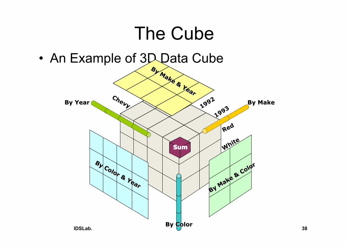
The Cube • An Example of 3D Data Cube
IDSLab. 38
By Year By Make
By Color
Sum

Cube: Each AWribute is a Dimension • N-dimensional Aggregate (sum(), max(),...)
– Fits relational model exactly: • a1, a2, ...., aN, f()
• Super-aggregate over N-1 Dimensional sub-cubes • ALL, a2, ...., aN , f() • a3 , ALL, a3, ...., aN , f() • ... • a1, a2, ...., ALL, f()
– This is the N-1 Dimensional cross-tab. • Super-aggregate over N-2 Dimensional sub-cubes
• ALL, ALL, a3, ...., aN , f() • ... • a1, a2 ,...., ALL, ALL, f()

The Data Cube Concept
MAKE
YEAR
COLOR
Ford
Chevy
Black
White
1994 1995
1994 1995
B
W
C
F
F
C
B W
F
C 1994
1995
B W
1994 1995

Sub-cube Derivation
• Dimension collapse, * denotes ALL
<M,Y,C>
<M,Y,*> <M,*,C> <*,Y,C>
<M,*,*> <*,Y,*> <*,*,C>
<*,*,*>

42 IDSLab. 42
CUBE Operator Possible syntax
• Proposed syntax example: – SELECT Model, Make, Year, SUM(Sales) FROM Sales WHERE Model IN {“Chevy”, “Ford”} AND Year BETWEEN 1990 AND 1994 GROUP BY CUBE Model, Make, Year HAVING SUM(Sales) > 0;
– Note: GROUP BY operator repeats aggregate list • in select list • in group by list

43
Cube Operator Example
SALES Model Year Color Sales Chevy 1990 red 5 Chevy 1990 white 87 Chevy 1990 blue 62 Chevy 1991 red 54 Chevy 1991 white 95 Chevy 1991 blue 49 Chevy 1992 red 31 Chevy 1992 white 54 Chevy 1992 blue 71 Ford 1990 red 64 Ford 1990 white 62 Ford 1990 blue 63 Ford 1991 red 52 Ford 1991 white 9 Ford 1991 blue 55 Ford 1992 red 27 Ford 1992 white 62 Ford 1992 blue 39
DATA CUBE Model Year Color Sales ALL ALL ALL 942 chevy ALL ALL 510 ford ALL ALL 432 ALL 1990 ALL 343 ALL 1991 ALL 314 ALL 1992 ALL 285 ALL ALL red 165 ALL ALL white 273 ALL ALL blue 339 chevy 1990 ALL 154 chevy 1991 ALL 199 chevy 1992 ALL 157 ford 1990 ALL 189 ford 1991 ALL 116 ford 1992 ALL 128 chevy ALL red 91 chevy ALL white 236 chevy ALL blue 183 ford ALL red 144 ford ALL white 133 ford ALL blue 156 ALL 1990 red 69 ALL 1990 white 149 ALL 1990 blue 125 ALL 1991 red 107 ALL 1991 white 104 ALL 1991 blue 104 ALL 1992 red 59 ALL 1992 white 116 ALL 1992 blue 110
CUBE
44 IDSLab. 44
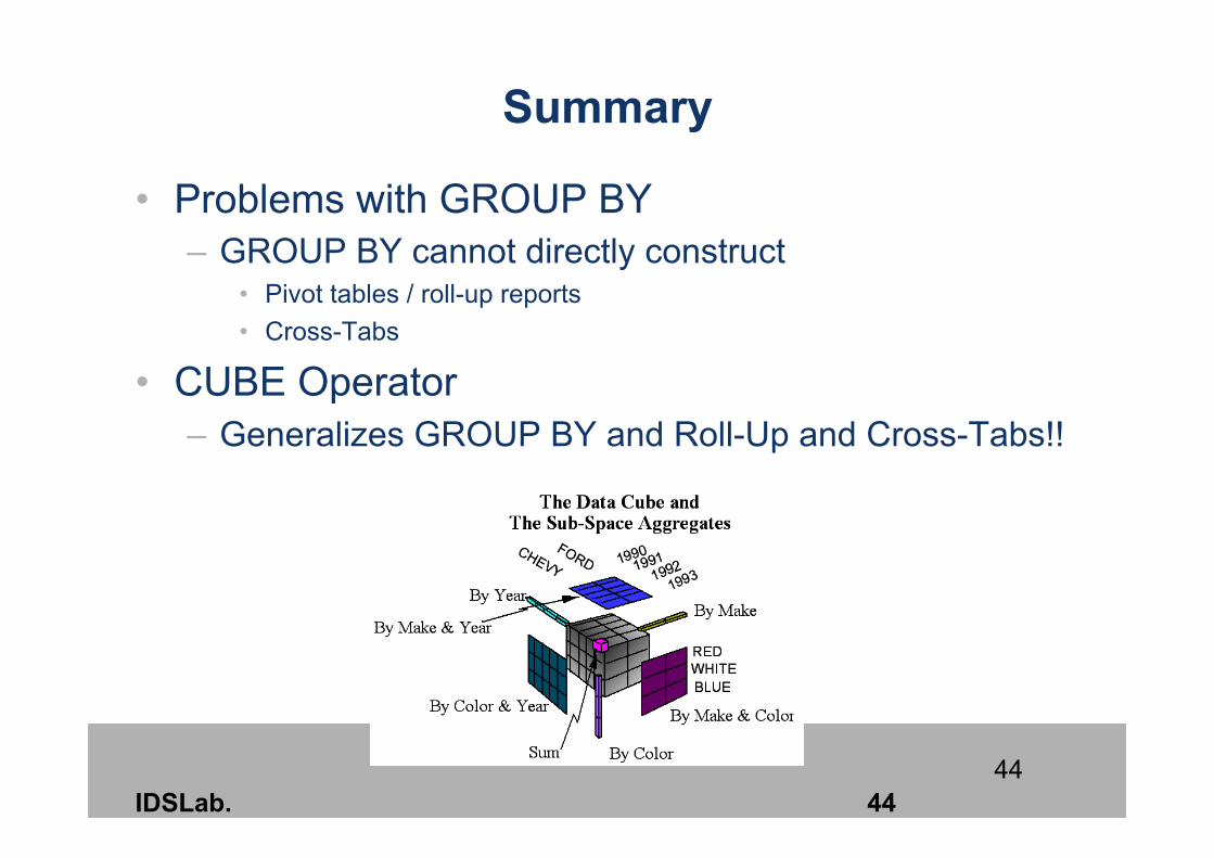
Summary
• Problems with GROUP BY – GROUP BY cannot directly construct
• Pivot tables / roll-up reports • Cross-Tabs
• CUBE Operator – Generalizes GROUP BY and Roll-Up and Cross-Tabs!!

Slicing
May 13, 2015 Data Mining: Concepts and
Techniques 45

Dicing
May 13, 2015 Data Mining: Concepts and
Techniques 46

Drill-up and Drill-Down
May 13, 2015 Data Mining: Concepts and
Techniques 47

Pivoting
May 13, 2015 Data Mining: Concepts and
Techniques 48

n Roll-up: A roll-up involves summarizing the data along a dimension. The summarization rule might be computing totals along a hierarchy or applying a set of formulas such as "profit = sales - expenses".[5]
May 13, 2015 Data Mining: Concepts and
Techniques 49

50 IDSLab.
Rollup Operator
• ROLLUP Operator: special case of CUBE Operator Return “Sales Roll Up by Store by Quarter” in 1994.: SELECT Store, quarter, SUM(Sales)
FROM Sales
WHERE nation=“Korea” AND Year=1994
GROUP BY ROLLUP Store, Quarter(Date) AS quarter;

OLAP GLOSSARY Defined terms: AGGREGATE ANALYSIS, MULTI-DIMENSIONAL ARRAY, MULTI-DIMENSIONAL CALCULATED MEMBER CELL CHILDREN COLUMN DIMENSION CONSOLIDATE CUBE DENSE DERIVED DATA DERIVED MEMBERS DETAIL MEMBER DIMENSION DRILL DOWN/UP FORMULA FORMULA, CROSS-DIMENSIONAL GENERATION, HIERARCHICAL HIERARCHICAL RELATIONSHIPS HORIZONTAL DIMENSION HYPERCUBE INPUT MEMBERS LEVEL, HIERARCHICAL MEMBER, DIMENSION MEMBER COMBINATION
MISSING DATA, MISSING VALUE MULTI-DIMENSIONAL DATA STRUCTURE MULTI-DIMENSIONAL QUERY LANGUAGE NAVIGATION NESTING (OF MULTI-DIMENSIONAL COLUMNS AND ROWS) NON-MISSING DATA OLAP CLIENT PAGE DIMENSION PAGE DISPLAY PARENT PIVOT PRE-CALCULATED/PRE-CONSOLIDATED DATA REACH THROUGH ROLL-UP ROTATE ROW DIMENSION SCOPING SELECTION SLICE SLICE AND DICE SPARSE VERTICAL DIMENSION
http://www.olapcouncil.org/research/glossaryly.htm

52
https://wicn.nssc.nasa.gov/

OLAP Screen Example
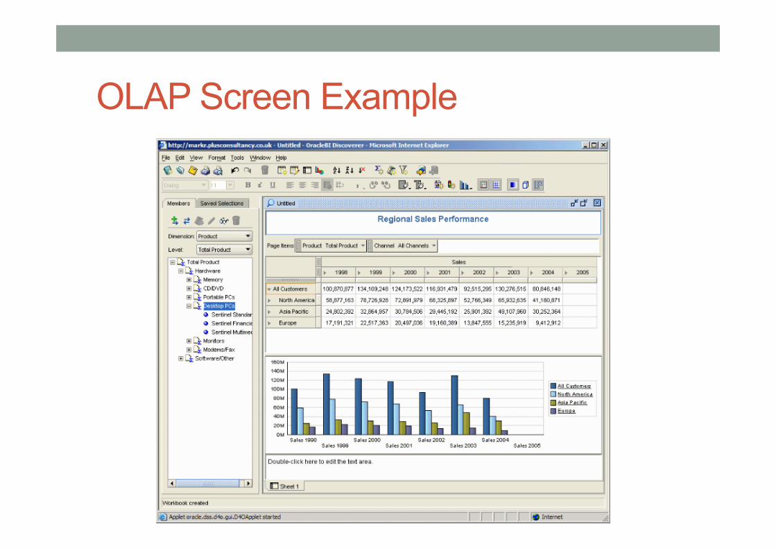
OLAP Screen Example

3. Multidimensional modelling

56
Multidimensional Data
• Sales volume as a function of product, month, and region
Prod
uct
Dimensions: Product, Location, Time Hierarchical summarization paths
Industry Region Year Category Country Quarter Product City Month Week Office Day
J. Han: Data Mining: Concepts and Techniques

Hector Garcia Molina: Data Warehousing and OLAP 57
Star
customer custId name address city53 joe 10 main sfo81 fred 12 main sfo
111 sally 80 willow la
product prodId name pricep1 bolt 10p2 nut 5
store storeId cityc1 nycc2 sfoc3 la
sale oderId date custId prodId storeId qty amto100 1/7/97 53 p1 c1 1 12o102 2/7/97 53 p2 c1 2 11105 3/8/97 111 p1 c3 5 50

Hector Garcia Molina: Data Warehousing and OLAP 58
Star Schema
saleorderIddatecustIdprodIdstoreIdqtyamt
customercustIdnameaddresscity
productprodIdnameprice
storestoreIdcity

Hector Garcia Molina: Data Warehousing and OLAP 59
Terms
● Fact table ● Dimension tables ● Measures sale
orderIddatecustIdprodIdstoreIdqtyamt
customercustIdnameaddresscity
productprodIdnameprice
storestoreIdcity

Hector Garcia Molina: Data Warehousing and OLAP 60
Dimension Hierarchies
store storeId cityId tId mgrs5 sfo t1 joes7 sfo t2 freds9 la t1 nancy
city cityId pop regIdsfo 1M northla 5M south
region regId namenorth cold regionsouth warm region
sType tId size locationt1 small downtownt2 large suburbs
store sType
city region
è snowflake schema è constellations
Hector Garcia Molina: Data Warehousing and OLAP 61
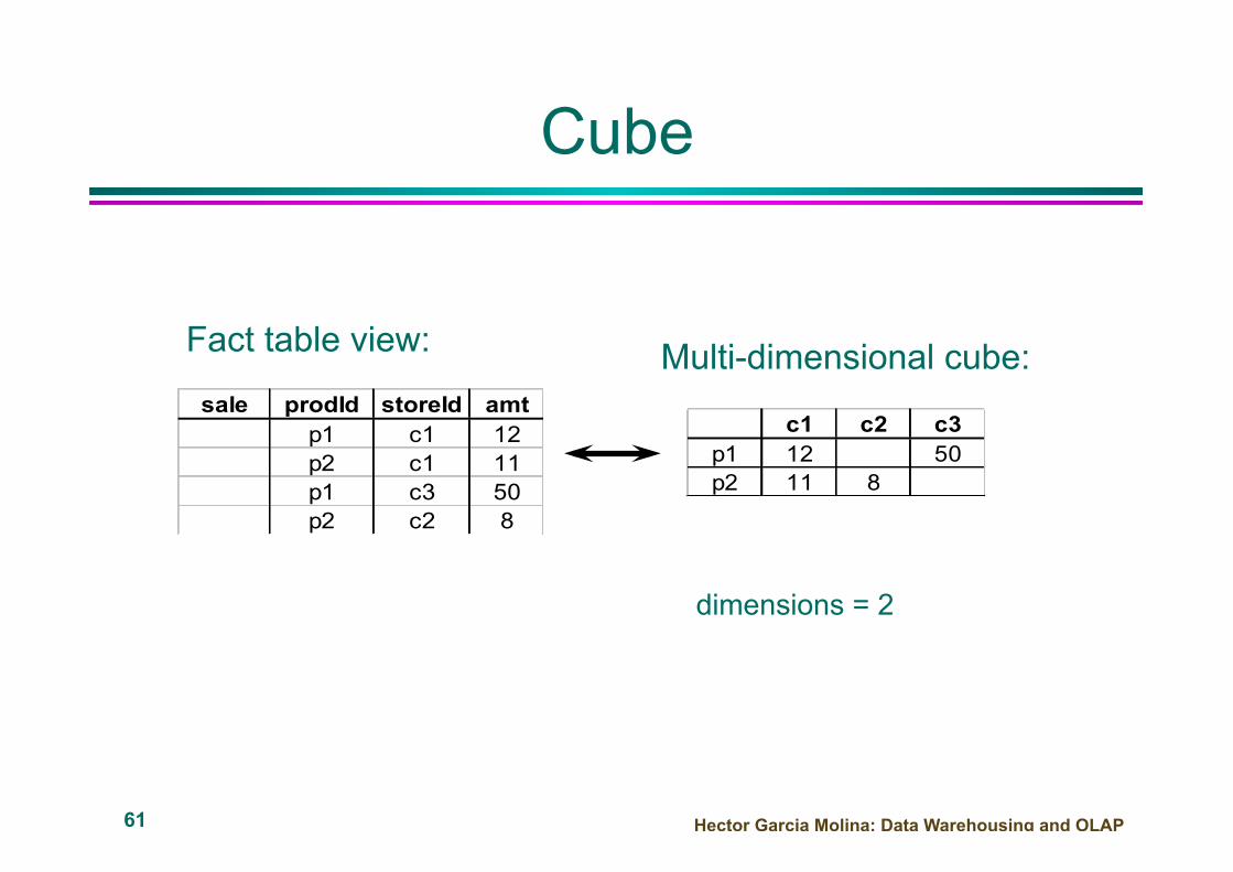
Cube
sale prodId storeId amtp1 c1 12p2 c1 11p1 c3 50p2 c2 8
c1 c2 c3p1 12 50p2 11 8
Fact table view: Multi-dimensional cube:
dimensions = 2

Hector Garcia Molina: Data Warehousing and OLAP 62
3-D Cube
sale prodId storeId date amtp1 c1 1 12p2 c1 1 11p1 c3 1 50p2 c2 1 8p1 c1 2 44p1 c2 2 4
day 2 c1 c2 c3p1 44 4p2 c1 c2 c3
p1 12 50p2 11 8
day 1
dimensions = 3
Multi-dimensional cube: Fact table view:

63
Star Schema
time_key day day_of_the_week month quarter year
time
location_key street city state_or_province country
location
Sales Fact Table
time_key
item_key
branch_key
location_key
units_sold
dollars_sold
avg_sales Measures
item_key item_name brand type supplier_type
item
branch_key branch_name branch_type
branch
J. Han: Data Mining: Concepts and Techniques

64
Snowflake Schema
time_key day day_of_the_week month quarter year
time
location_key street city_key
location
Sales Fact Table
time_key
item_key
branch_key
location_key
units_sold
dollars_sold
avg_sales
Measures
item_key item_name brand type supplier_key
item
branch_key branch_name branch_type
branch
supplier_key supplier_type
supplier
city_key city state_or_province country
city
J. Han: Data Mining: Concepts and Techniques

Case study: Hospital What is data warehouse • InformaEon system for reporEng purposes • The goal is to fulfill reporEng needs which are unsaEsfied in operaEonal system • It is easy to modify old and design new reports
• No „write spec to so]ware developer to get the report“ anymore
• Reports can be filled with data quickly • No „start the report generaEon at night to prevent system load“ anymore
• The data comes from operaEonal system(s)

Goal of the work package
• Work out the main concepts for building data warehouse for hospital IS • What are the reporEng needs? • What are the data cubes that cover most reporEng needs for „universal“ hospital?
• How to get the data into these cubes?
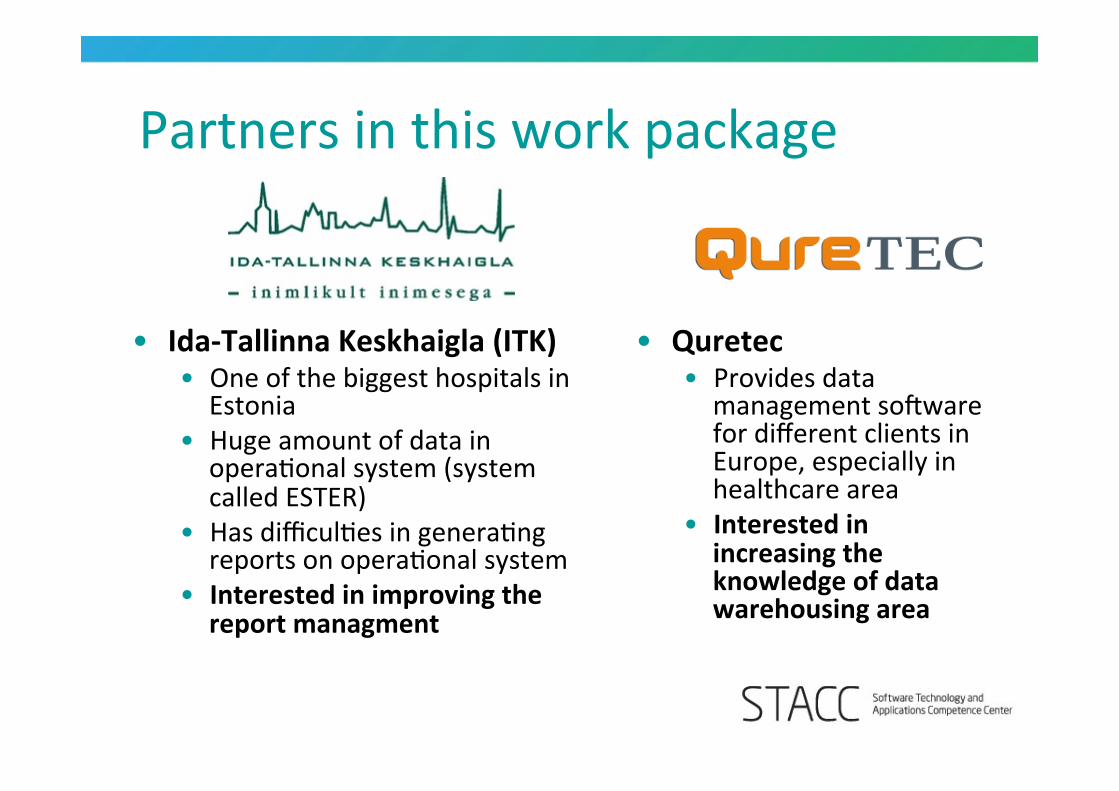
Partners in this work package
• Ida-‐Tallinna Keskhaigla (ITK) • One of the biggest hospitals in Estonia
• Huge amount of data in operaEonal system (system called ESTER)
• Has difficulEes in generaEng reports on operaEonal system
• Interested in improving the report managment
• Quretec • Provides data management so]ware for different clients in Europe, especially in healthcare area
• Interested in increasing the knowledge of data warehousing area

So far... (1)
• We have analyzed the data and data structures in operaEonal system

So far...(2)
• We have designed the interface for geeng the data from ESTER
• We have built 2 data cubes
OperaEonal IS
SQL view
„Interface“ for building data
cubes Data cubes
Reports Data in operaEonal
IS
SQL view

So far... (3)
• We have designed 10 reports on the data cubes

So far... (4)
• Showed that report generaEon Eme has reduced from tens of minutes to few seconds
Selected period Number of pa4ents
Seconds for genera4ng report in opera4onal
system
Seconds for genera4ng the same report in data
warehouse 1 day 138 149 1
1 month 2944 150 1
1 year 32286 584 1

So far... (5)
• We showed that data warehouse offers addiEonal benefits: • MulEple output formats • Reports can be redesigned easily • New combined reports -‐> new value from the data
Hector Garcia Molina: Data Warehousing and OLAP 73
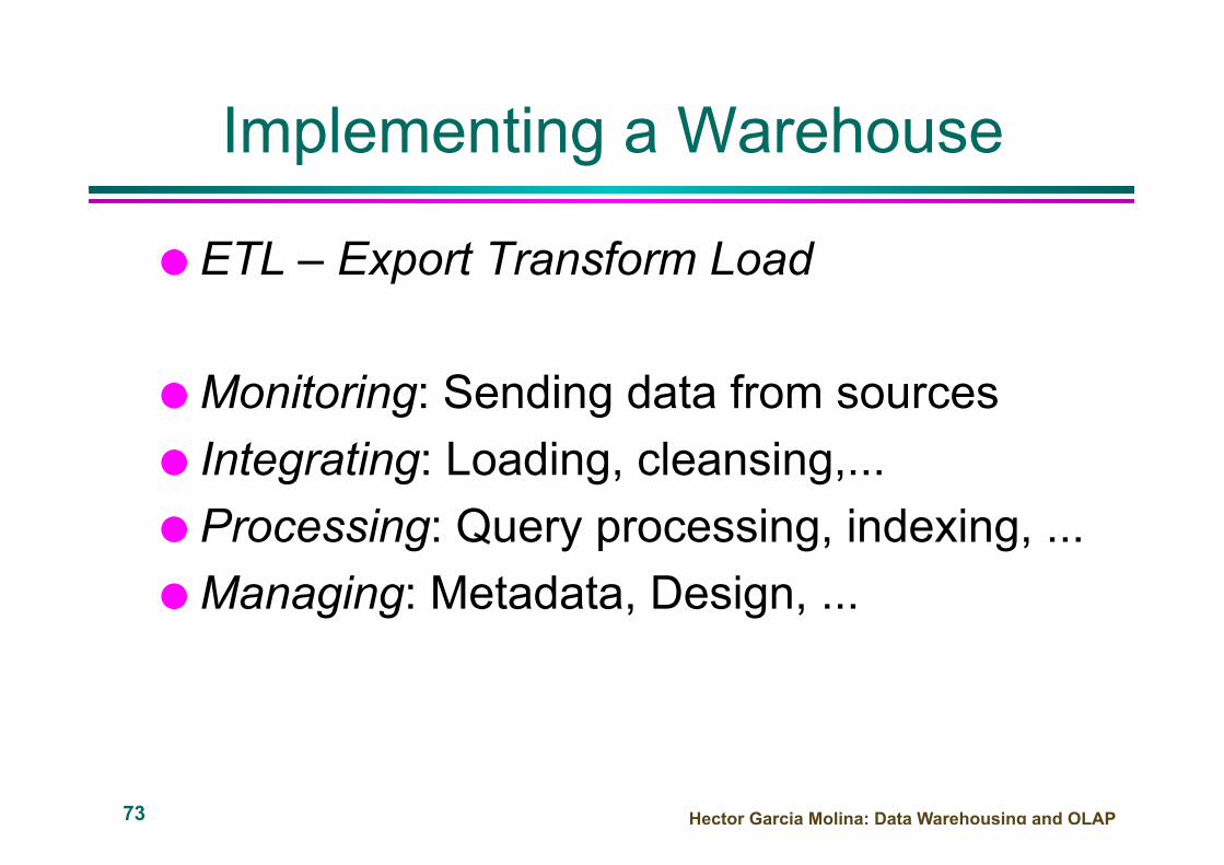
Implementing a Warehouse
● ETL – Export Transform Load
● Monitoring: Sending data from sources ● Integrating: Loading, cleansing,... ● Processing: Query processing, indexing, ... ● Managing: Metadata, Design, ...

Hector Garcia Molina: Data Warehousing and OLAP 74
Monitoring
● Source Types: relational, flat file, IMS, VSAM, IDMS, WWW, news-wire, …
● Incremental vs. Refresh
customer id name address city53 joe 10 main sfo81 fred 12 main sfo
111 sally 80 willow la new

Hector Garcia Molina: Data Warehousing and OLAP 75
Monitoring Techniques
● Periodic snapshots ● Database triggers ● Log shipping ● Data shipping (replication service) ● Transaction shipping ● Polling (queries to source) ● Screen scraping ● Application level monitoring
è
Adv
anta
ges
& D
isad
vant
ages
!!
Hector Garcia Molina: Data Warehousing and OLAP 76
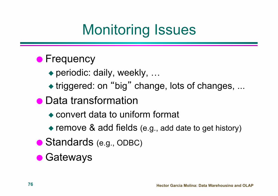
Monitoring Issues
● Frequency ◆ periodic: daily, weekly, … ◆ triggered: on “big” change, lots of changes, ...
● Data transformation ◆ convert data to uniform format ◆ remove & add fields (e.g., add date to get history)
● Standards (e.g., ODBC) ● Gateways
Hector Garcia Molina: Data Warehousing and OLAP 77
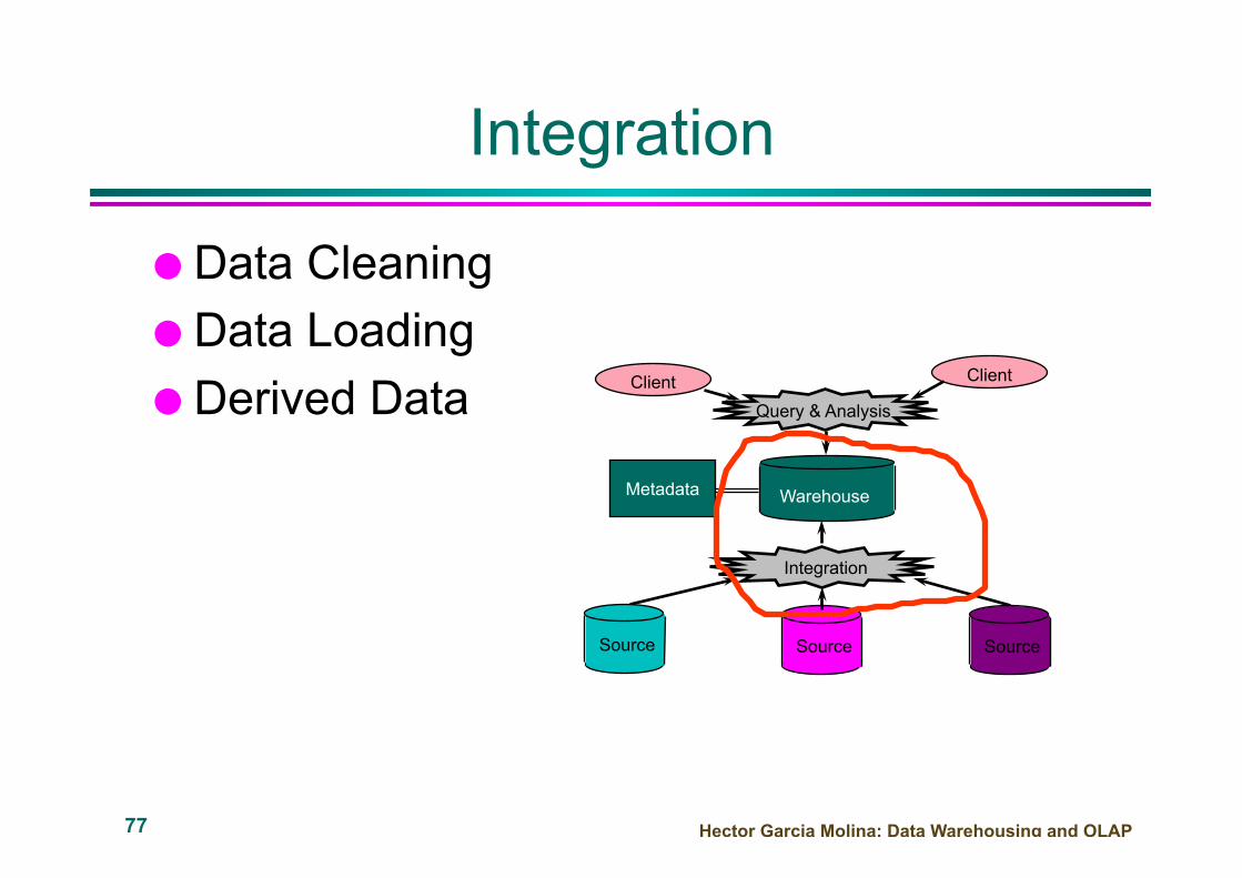
Integration
● Data Cleaning ● Data Loading ● Derived Data Client Client
Warehouse
Source Source Source
Query & Analysis
Integration
Metadata

Hector Garcia Molina: Data Warehousing and OLAP 78
Data Cleaning
● Migration (e.g., yen ð dollars) ● Scrubbing: use domain-specific knowledge (e.g.,
social security numbers) ● Fusion (e.g., mail list, customer merging) ● Auditing: discover rules & relationships
(like data mining)
billing DB
service DB
customer1(Joe)
customer2(Joe)
merged_customer(Joe)

Hector Garcia Molina: Data Warehousing and OLAP 79
Loading Data
● Incremental vs. refresh ● Off-line vs. on-line ● Frequency of loading
◆ At night, 1x a week/month, continuously ● Parallel/Partitioned load
Hector Garcia Molina: Data Warehousing and OLAP 80
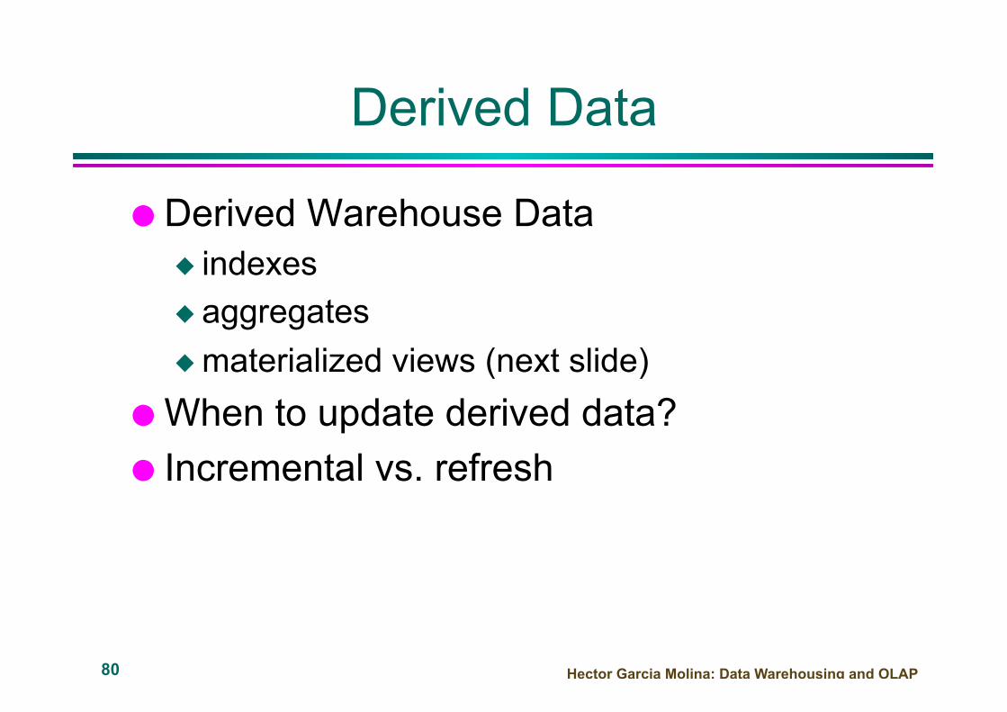
Derived Data
● Derived Warehouse Data ◆ indexes ◆ aggregates ◆ materialized views (next slide)
● When to update derived data? ● Incremental vs. refresh

ETL
● Export
● Transform
● Load
81

Hector Garcia Molina: Data Warehousing and OLAP 82
Design
● What data is needed? ● Where does it come from? ● How to clean data? ● How to represent in warehouse (schema)? ● What to summarize? ● What to materialize? ● What to index?

Hector Garcia Molina: Data Warehousing and OLAP 83
ROLAP Server
● Relational OLAP Server
relational DBMS
ROLAP server
tools
utilities
sale prodId date sump1 1 62p2 1 19p1 2 48
Special indices, tuning; Schema is “denormalized”

Hector Garcia Molina: Data Warehousing and OLAP 84
MOLAP Server
● Multi-Dimensional OLAP Server
multi-dimensional
server
M.D. tools
utilities could also
sit on relational
DBMS
Prod
uct
Date 1 2 3 4
milk soda eggs soap
A B Sales

Hector Garcia Molina: Data Warehousing and OLAP 85
Index Structures
● Traditional Access Methods ◆ B-trees, hash tables, R-trees, grids, …
● Popular in Warehouses ◆ inverted lists ◆ bit map indexes ◆ join indexes ◆ text indexes

Hector Garcia Molina: Data Warehousing and OLAP 86
Inverted Lists
2023
1819
202122
232526
r4r18r34r35
r5r19r37r40
rId name ager4 joe 20r18 fred 20r19 sally 21r34 nancy 20r35 tom 20r36 pat 25r5 dave 21r41 jeff 26
. . .
age index
inverted lists
data records

Hector Garcia Molina: Data Warehousing and OLAP 87
Using Inverted Lists
● Query: ◆ Get people with age = 20 and name = “fred”
● List for age = 20: r4, r18, r34, r35 ● List for name = “fred”: r18, r52 ● Answer is intersection: r18
Hector Garcia Molina: Data Warehousing and OLAP 88
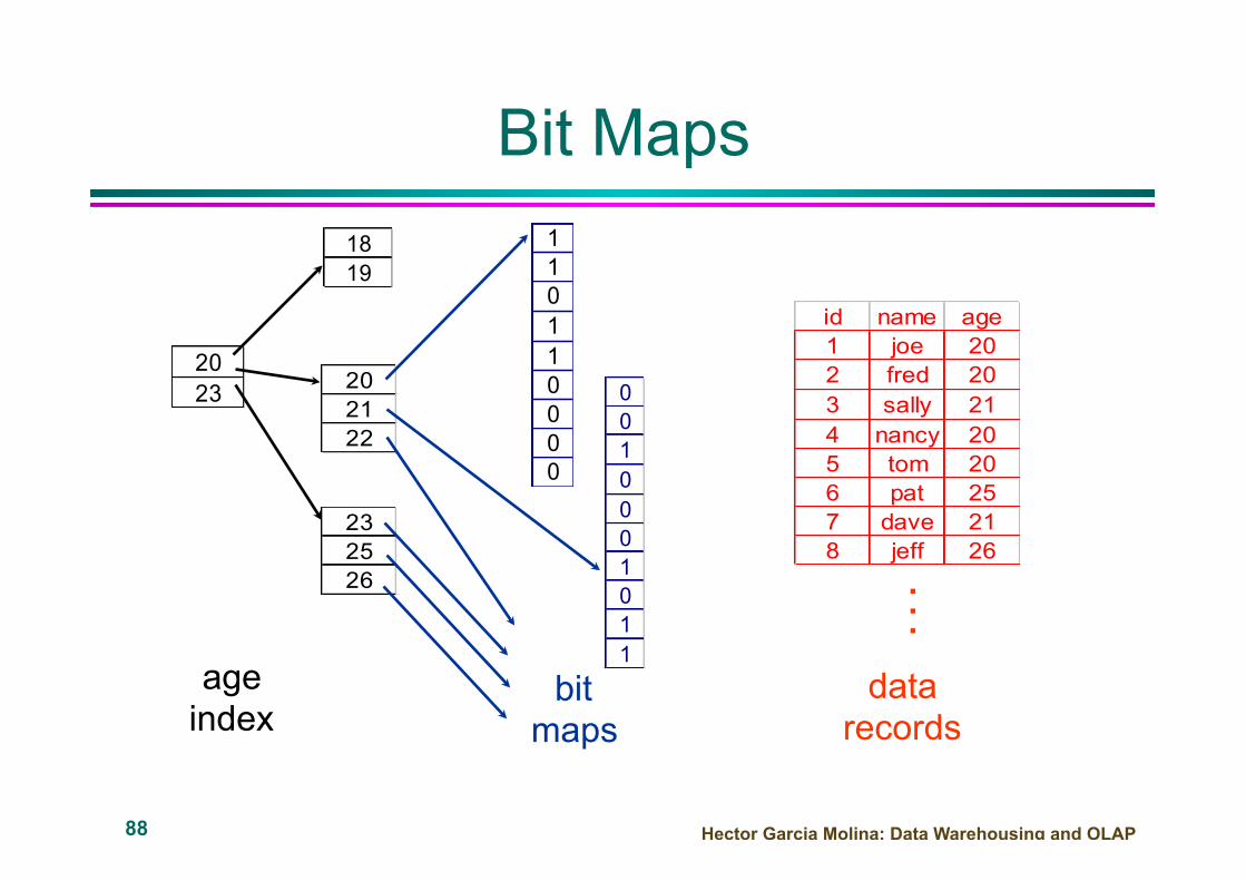
Bit Maps
2023
1819
202122
232526
id name age1 joe 202 fred 203 sally 214 nancy 205 tom 206 pat 257 dave 218 jeff 26
. . .
age index
bit maps
data records
110110000
0010001011

Hector Garcia Molina: Data Warehousing and OLAP 89
Using Bit Maps
● Query: ◆ Get people with age = 20 and name = “fred”
● List for age = 20: 1101100000 ● List for name = “fred”: 0100000001 ● Answer is intersection: 010000000000
● Good if domain cardinality small ● Bit vectors can be compressed

Hector Garcia Molina: Data Warehousing and OLAP 90
Join
sale prodId storeId date amtp1 c1 1 12p2 c1 1 11p1 c3 1 50p2 c2 1 8p1 c1 2 44p1 c2 2 4
• “Combine” SALE, PRODUCT relations • In SQL: SELECT * FROM SALE, PRODUCT
product id name pricep1 bolt 10p2 nut 5
joinTb prodId name price storeId date amtp1 bolt 10 c1 1 12p2 nut 5 c1 1 11p1 bolt 10 c3 1 50p2 nut 5 c2 1 8p1 bolt 10 c1 2 44p1 bolt 10 c2 2 4

Hector Garcia Molina: Data Warehousing and OLAP 91
Join Indexes
product id name price jIndexp1 bolt 10 r1,r3,r5,r6p2 nut 5 r2,r4
sale rId prodId storeId date amtr1 p1 c1 1 12r2 p2 c1 1 11r3 p1 c3 1 50r4 p2 c2 1 8r5 p1 c1 2 44r6 p1 c2 2 4
join index
Hector Garcia Molina: Data Warehousing and OLAP 92
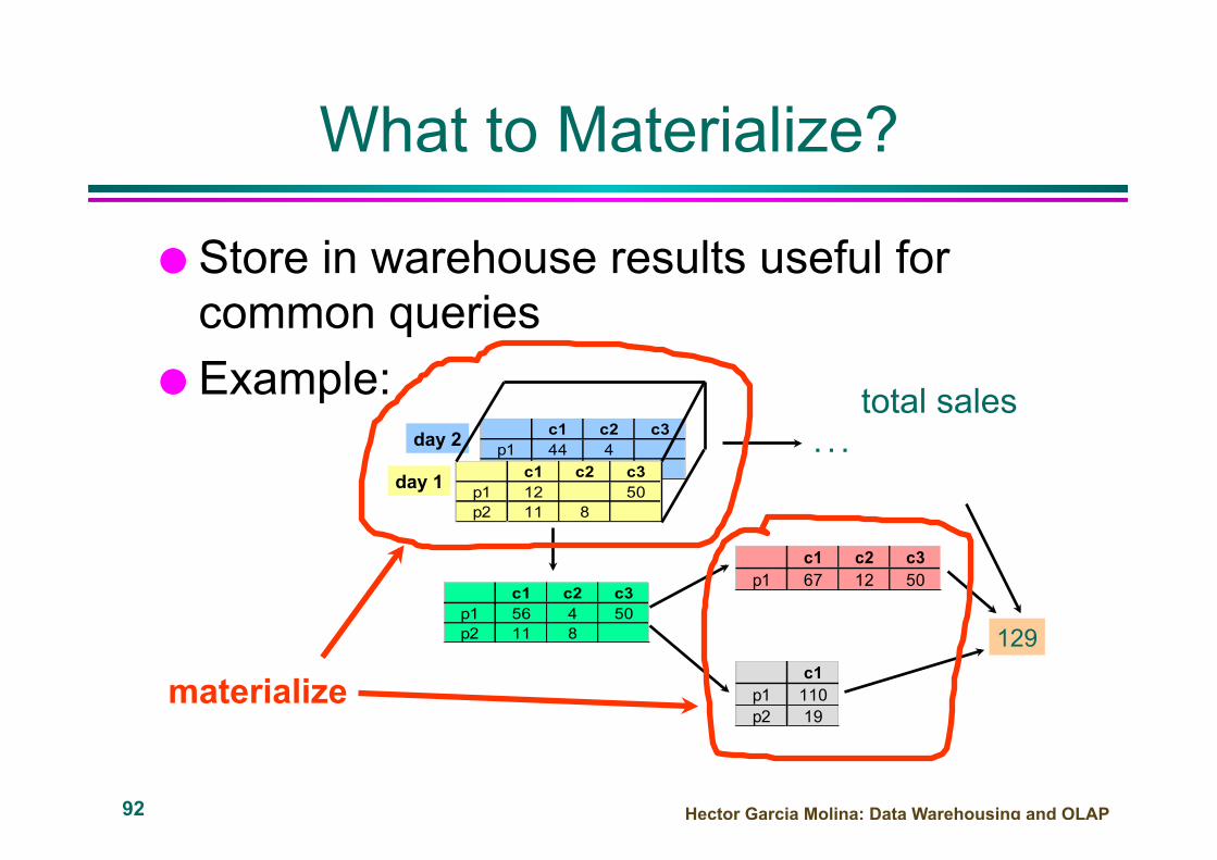
What to Materialize?
● Store in warehouse results useful for common queries
● Example: day 2 c1 c2 c3
p1 44 4p2 c1 c2 c3
p1 12 50p2 11 8
day 1
c1 c2 c3p1 56 4 50p2 11 8
c1 c2 c3p1 67 12 50
c1p1 110p2 19
129
. . . total sales
materialize

Hector Garcia Molina: Data Warehousing and OLAP 93
Materialization Factors
● Type/frequency of queries ● Query response time ● Storage cost ● Update cost

Hector Garcia Molina: Data Warehousing and OLAP 94
Cube Aggregates Lattice
city, product, date
city, product city, date product, date
city product date
all
day 2 c1 c2 c3p1 44 4p2 c1 c2 c3
p1 12 50p2 11 8
day 1
c1 c2 c3p1 56 4 50p2 11 8
c1 c2 c3p1 67 12 50
129
use greedy algorithm to decide what to materialize

Hector Garcia Molina: Data Warehousing and OLAP 95
Interesting Hierarchy
all
years
quarters
months
days
weeks
time day week month quarter year1 1 1 1 20002 1 1 1 20003 1 1 1 20004 1 1 1 20005 1 1 1 20006 1 1 1 20007 1 1 1 20008 2 1 1 2000
conceptual dimension table

Aalborg University 2012 - DataInt! 96!
Changing Dimensions!
• So far, we assumed that dimensions are stable over time"n New rows in dimension tables can be inserted"n Existing rows do not change"
◆ This is not a realistic assumption"• We now study techniques for handling changes in
dimensions"• “Slowly changing dimensions” phenomenon"
n Dimension information change, but changes are not frequent"
n Still assume that the schema is fixed"

Aalborg University 2012 - DataInt! 97!
Advanced: Handling Changes in Dimensions!
• Handling change over time"• Changes in dimensions"
n 1. No special handling"n 2. Versioning dimension values"
◆ 2A. Special facts"◆ 2B. Timestamping"
n 3. Capturing the previous and the current value"n 4. Split into changing and constant attributes"

Aalborg University 2012 - DataInt! 98!
Example"
• Attribute values in dimensions vary over time"n A store changes Size"n A product changes
Description"n Districts are changed"
• Problems "n Dimensions not updated
è DW is not up-to-date"n Dimensions updated in a
straightforward way è incorrect information in historical data"
TimeID!StoreID!ProductID!…"ItemsSold"Amount" ProductID!
Description"Brand"PCategory"
StoreID!Address"City "District"Size"SCategory"
TimeID!Weekday"Week"Month"Quarter"Year"DayNo"Holiday"
timeline"
change"?" ?"
Sales fact"
Time dim."Store dim."
Product dim."

Aalborg University 2012 - DataInt! 99!
Example"
TimeID!StoreID!ProductID!…"ItemsSold"Amount"
…"
StoreID!Address"City "District"Size"SCategory"
…"Sales fact"
Time dim."Store dim."
Product dim."
2000"ItemsSold"
001"…"…"StoreID "
250"Size"
001"…"…"StoreID"
Sales fact table" Store dimension table"
The store in Aalborg has "the size of 250 sq. metres.""On a certain day,"customers bought 2000"apples from that store."

Aalborg University 2012 - DataInt! 100!
Solution 1: No Special Handling"
2000"ItemsSold"
001"…"…"StoreID "
250"Size"
001"…"…"StoreID"
2000"ItemsSold"
001"…"…"StoreID"
450"Size"
001"…"…"StoreID"
2000"001"3500"
ItemsSold"
001"
…"…"StoreID"450"Size"
001"…"…"StoreID"
Sales fact table" Store dimension table"
The size of a store expands"
A new fact arrives"
What’s the problem here?"

Aalborg University 2012 - DataInt! 101!
Solution 1"• Solution 1: Overwrite the old values in the
dimension tables"• Consequences"
n Old facts point to rows in the dimension tables with incorrect information!"
n New facts point to rows with correct information"
• Pros"n Easy to implement"n Useful if the updated attribute is not significant, or the old
value should be updated for error correction"• Cons"
n Old facts may point to “incorrect” rows in dimensions"

Aalborg University 2012 - DataInt! 102!
Solution 2"• Solution 2: Versioning of rows with changing attributes"
n The key that links dimension and fact table, identifies a version of a row, not just a “row”"
n Surrogate keys make this easier to implement"◆ – what if we had used, e.g., the shop’s zip code as key?"◆ Always use surrogate keys!!!"
• Consequences"n Larger dimension tables"
• Pros"n Correct information captured in DW"n No problems when formulating queries"
• Cons"n Cannot capture the development over time of the subjects the
dimensions describe in the simplest form (but we can fix that)"

Aalborg University 2012 - DataInt! 103!
Solution 2: Versioning of Rows"StoreID" …" ItemsSold" …"001" 2000"
StoreID" …" Size" …"001" 250"
StoreID" …" ItemsSold" …"001" 2000"
StoreID" …" Size" …"001" 250"002" 450"
StoreID" …" ItemsSold" …"001" 2000"002" 3500"
StoreID" …" Size" …"001" 250"002" 450"
different versions of a store"
Which store does the "new fact (old fact) refer to?"
A new fact arrives"

Aalborg University 2012 - DataInt! 104!
Solution 2A"
• Solution 2A: Use special facts for capturing changes in dimensions via the Time dimension"n Assume that no simultaneous, new fact refers to the
new dimension row"n Insert a new special fact that points to the new
dimension row, and through its reference to the Time dimension, timestamps the row "
• Pros"n Possible to capture the development over time of the
subjects that the dimensions describe"• Cons"
n Larger fact table"n Cumbersome to use special facts in queries"

Aalborg University 2012 - DataInt! 105!
Solution 2A: Inserting Special Facts"
StoreID" TimeID" … ItemsSold" …"001" 234" 2000"
StoreID" …" Size" …"001" 250"
StoreID" …" Size" …"001" 250"002" 450"
StoreID" …" Size" …"001" 250"002" 450"
StoreID" TimeID" … ItemsSold" …"001" 234" 2000"002" 345" -"
StoreID" TimeID" … ItemsSold" …"001" 234" 2000"002" 345" -"002" 456" 3500"
special fact for capturing changes"

Aalborg University 2012 - DataInt! 106!
Solution 2B"
• Solution 2B: Versioning of rows with changing attributes like in Solution 2 + timestamping of rows in the slowly changing dimension (SCD) with From and To attributes"
• Pros"n Correct information captured in DW"
• Cons"n Larger dimension tables"

Aalborg University 2012 - DataInt! 107!
Solution 2B: Timestamping"
StoreID" TimeID" … ItemsSold" …"001" 234" 2000"
StoreID" Size" From" To"001" 250" 1998" -"
StoreID" TimeID" … ItemsSold" …"001" 234" 2000"
StoreID" TimeID" … ItemsSold" …"001" 234" 2000"002" 456" 3500"
StoreID" Size" From" To"001" 250" 1998" 1999"002" 450" 2000" -"
StoreID" Size" From" To"001" 250" 1998" 1999"002" 450" 2000" -"
attributes: “From”, “To”"

Aalborg University 2012 - DataInt! 108!
Example of Using Solution 2B"
• Product descriptions are versioned, when products are changed, e.g., new package sizes"n Old versions are still in the stores, new facts can refer
to both the newest and older versions of products"n Time value for a fact not necessarily between “From”
and “To” values in the fact’s Product dimension row"• Unlike changes in Size for a store, where all facts
from a certain point in time will refer to the newest Size value"
• Unlike alternative categorizations that one wants to choose between"

Aalborg University 2012 - DataInt! 109!
Solution 3"• Solution 3: Create two versions of each changing attribute"
n One attribute contains the current value"n The other attribute contains the previous value"
• Consequences"n Two values are attached to each dimension row"
• Pros"n Possible to compare across the change in dimension value (which
is a problem with Solution 2)"◆ Such comparisons are interesting when we need to work
simultaneously with two alternative values"◆ Example: Categorization of stores and products"
• Cons"n Not possible to see when the old value changed to the new"n Only possible to capture the two latest values"

Aalborg University 2012 - DataInt! 110!
Solution 3: Two versions of Changing Attribute"
StoreID" …" ItemsSold" …"001" 2000"
StoreID" …" DistrictOld" DistrictNew" …001" 37" 37"
StoreID" …" ItemsSold" …"001" 2000"
StoreID" …" ItemsSold" …"001" 2000"001" 2100"
StoreID" …" DistrictOld" DistrictNew" …001" 37" 73"
StoreID" …" DistrictOld" DistrictNew" …001" 37" 73"
versions of an attribute"
We cannot find out when the district changed."

Aalborg University 2012 - DataInt! 111!
Rapidly Changing Dimensions"• Difference between “slowly” and “rapidly” is subjective"
n Solution 2 is often still feasible"n The problem is the size of the dimension"
• Example"n Assume an Employee dimension with 100,000 employees, each
using 2K bytes and many changes every year"n Solution 2B is recommended"
• Examples of (large) dimensions with many changes: Product and Customer"
• The more attributes in a dimension table, the more changes per row are expected"
• Example"n A Customer dimension with 100M customers and many attributes"n Solution 2 yields a dimension that is too large"

Aalborg University 2012 - DataInt! 112!
Solution 4: Dimension Splitting"
CustID"Name"PostalAddress"Gender"DateofBirth"Customerside"…"NoKids"MaritialStatus"CreditScore"BuyingStatus"Income"Education"…"
ProfileID"NoKids"MaritialStatus"CreditScoreGroup"BuyingStatusGroup"IncomeGroup"…"
CustID"Name"PostalAddress"Gender"DateofBirth"Customerside"…"
Customer dimension (original)" Customer dimension (new): "
"relatively static
attributes"
Profile dimension (not a SCD):"
"often-changing
attributes"

Aalborg University 2012 - DataInt! 113!
Solution 4"• Solution 4"
n Make a “minidimension” with the often-changing attributes"n Convert (numeric) attributes with many possible values into
attributes with few discrete or banded values"◆ E.g., Income group: [0,10K), [0,20K), [0,30K), [0,40K)"◆ Why? Any Information Loss?!
n Insert rows for all combinations of values from these new domains"◆ With 6 attributes with 10 possible values each, the dimension gets
106=1,000,000 rows"◆ What do we do, if there are too many (theoretical) combinations?"
n If the minidimension is too large, it can be further split into more minidimensions"
◆ Here, synchronous/correlated attributes must be considered (to be placed in the same minidimension)"
◆ The same attribute can be repeated in another minidimension"

Aalborg University 2012 - DataInt! 114!
Solution 4 (Changing Dimensions)"
• Pros"n DW size (dimension tables) is kept down"n Changes in a customer’s profile values do not result in
changes in dimensions"• Cons"
n More dimensions and more keys in the star schema"n Navigation of customer attributes is more cumbersome
as these are in more than one dimension "n Using value groups gives less detail"n The construction of groups is irreversible"

Aalborg University 2012 - DataInt! 115!
Changing Dimensions - Summary"
• Why are there changes in dimensions?"n Applications change"n The modeled reality changes"
• Multidimensional models realized as star schemas support change over time to a large extent"
• A number of techniques for handling change over time at the instance level was described"n Solution 2 and the derived 2B are the most useful"n Possible to capture change precisely"

Hector Garcia Molina: Data Warehousing and OLAP 116
Tools
● Development ◆ design & edit: schemas, views, scripts, rules, queries, reports
● Planning & Analysis ◆ what-if scenarios (schema changes, refresh rates), capacity planning
● Warehouse Management ◆ performance monitoring, usage patterns, exception reporting
● System & Network Management ◆ measure traffic (sources, warehouse, clients)
● Workflow Management ◆ “reliable scripts” for cleaning & analyzing data

DW Products and Tools (old)
• Oracle 11g, IBM DB2, Microsoft SQL Server, ... – All provide OLAP extensions
• SAP Business Information Warehouse – ERP vendors
• MicroStrategy, Cognos (now IBM) – Specialized vendors – Kind of Web-based EXCEL
• Niche Players (e.g., Btell) – Vertical application domain

MDX (Multi-Dimensional eXpressions) " MDX is a Microsoft implementation of query
language for OLAP n http://msdn.microsoft.com/en-us/library/bb500184.aspx
" Example SELECT {[Dim Date].[Time Year].[Time Year]} ON COLUMNS, {[Dim Location].[Region].[Region]} ON ROWS FROM [Mini DW] WHERE ([Measures].[Sales Amount])
118
May 13, 2015 Data Mining: Concepts and
Techniques 119
Chapter 2: Data Preprocessing
n Why preprocess the data?
n Data cleaning
n Data integration and transformation
n Data reduction
n Discretization and concept hierarchy generation
n Summary

May 13, 2015 Data Mining: Concepts and
Techniques 120
Discretization
n Three types of attributes:
n Nominal — values from an unordered set, e.g., color, profession
n Ordinal — values from an ordered set, e.g., military or academic
rank
n Continuous — real numbers, e.g., integer or real numbers
n Discretization:
n Divide the range of a continuous attribute into intervals
n Some classification algorithms only accept categorical attributes.
n Reduce data size by discretization
n Prepare for further analysis

May 13, 2015 Data Mining: Concepts and
Techniques 121
Discretization and Concept Hierarchy
n Discretization
n Reduce the number of values for a given continuous attribute by dividing the range of the attribute into intervals
n Interval labels can then be used to replace actual data values
n Supervised vs. unsupervised
n Split (top-down) vs. merge (bottom-up)
n Discretization can be performed recursively on an attribute
n Concept hierarchy formation
n Recursively reduce the data by collecting and replacing low level concepts (such as numeric values for age) by higher level concepts (such as young, middle-aged, or senior)

May 13, 2015 Data Mining: Concepts and
Techniques 122
Segmentation by Natural Partitioning
n A simply 3-4-5 rule can be used to segment numeric data into relatively uniform, “natural” intervals.
n If an interval covers 3, 6, 7 or 9 distinct values at the
most significant digit, partition the range into 3 equi-width intervals
n If it covers 2, 4, or 8 distinct values at the most
significant digit, partition the range into 4 intervals
n If it covers 1, 5, or 10 distinct values at the most significant digit, partition the range into 5 intervals

May 13, 2015 Data Mining: Concepts and
Techniques 123
Example of 3-4-5 Rule
(-$400 -$5,000)
(-$400 - 0) (-$400 - -$300) (-$300 - -$200) (-$200 - -$100)
(-$100 - 0)
(0 - $1,000) (0 - $200) ($200 - $400)
($400 - $600)
($600 - $800) ($800 -
$1,000)
($2,000 - $5, 000)
($2,000 - $3,000)
($3,000 - $4,000)
($4,000 - $5,000)
($1,000 - $2, 000) ($1,000 - $1,200)
($1,200 - $1,400)
($1,400 - $1,600)
($1,600 - $1,800) ($1,800 -
$2,000)
msd=1,000 Low=-$1,000 High=$2,000 Step 2:
Step 4:
Step 1: -$351 -$159 profit $1,838 $4,700 Min Low (i.e, 5%-tile) High(i.e, 95%-0 tile) Max
count
(-$1,000 - $2,000)
(-$1,000 - 0) (0 -$ 1,000) Step 3:
($1,000 - $2,000)

Example
May 13, 2015 Data Mining: Concepts and Techniques 124
-351,976.00 .. 4,700,896.50 MIN=-351,976.00 MAX=4,700,896.50 LOW = 5th percentile -159,876 HIGH = 95th percentile 1,838,761 msd = 1,000,000 (most significant digit) LOW = -1,000,000 (round down) HIGH = 2,000,000 (round up) 3 value ranges 1. (-1,000,000 .. 0] 2. (0 .. 1,000,000] 3. (1,000,000 .. 2,000,000] Adjust with real MIN and MAX 1. (-400,000 .. 0] 2. (0 .. 1,000,000] 3. (1,000,000 .. 2,000,000] 4. (2,000,000 .. 5,000,000]

Jaak Vilo and other authors UT: Data Mining 2009 125
Recursive … 1.1. (-400,000 .. -300,000 ] 1.2. (-300,000 .. -200,000 ] 1.3. (-200,000 .. -100,000 ] 1.4. (-100,000 .. 0 ] 2.1. (0 .. 200,000 ] 2.2. (200,000 .. 400,000 ] 2.3. (400,000 .. 600,000 ] 2.4. (600,000 .. 800,000 ] 2.5. (800,000 .. 1,000,000 ] 3.1. (1,000,000 .. 1,200,000 ] 3.2. (1,200,000 .. 1,400,000 ] 3.3. (1,400,000 .. 1,600,000 ] 3.4. (1,600,000 .. 1,800,000 ] 3.5. (1,800,000 .. 2,000,000 ] 4.1. (2,000,000 .. 3,000,000 ] 4.2. (3,000,000 .. 4,000,000 ] 4.3. (4,000,000 .. 5,000,000 ]

Concept Hierarchy Generation for Categorical Data
• Specification of a partial/total ordering of attributes explicitly at the schema level by users or experts
– street < city < state < country • Specification of a hierarchy for a set of values by explicit
data grouping – {Urbana, Champaign, Chicago} < Illinois
• Specification of only a partial set of attributes – E.g., only street < city, not others
• Automatic generation of hierarchies (or attribute levels) by the analysis of the number of distinct values
– E.g., for a set of attributes: {street, city, state, country} May 13, 2015 Data Mining: Concepts and Techniques 126
May 13, 2015 Data Mining: Concepts and
Techniques 127
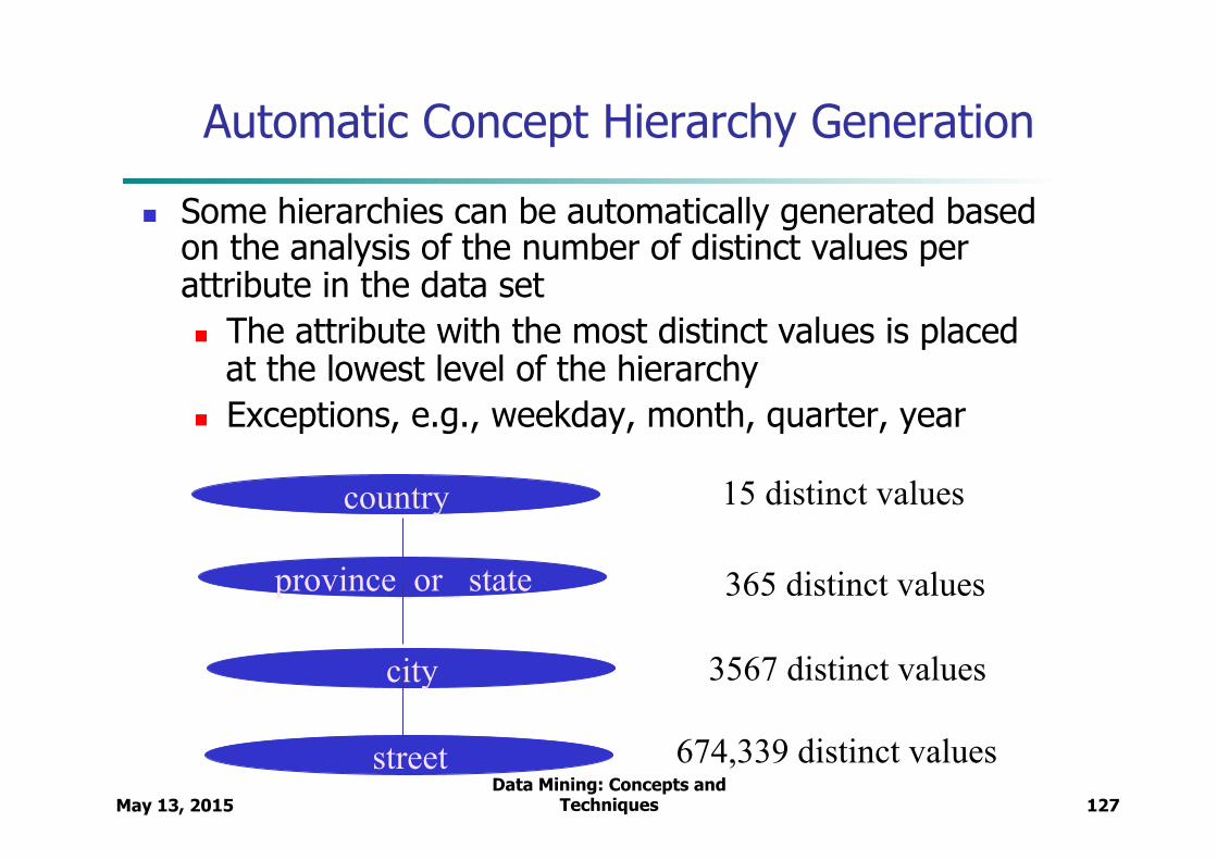
Automatic Concept Hierarchy Generation
n Some hierarchies can be automatically generated based on the analysis of the number of distinct values per attribute in the data set n The attribute with the most distinct values is placed
at the lowest level of the hierarchy n Exceptions, e.g., weekday, month, quarter, year
country
province_or_ state
city
street
15 distinct values
365 distinct values
3567 distinct values
674,339 distinct values

Summary
• OLAP and DW – a way to summarise data
• Prepare data for further data mining and visualisaEon
• Fact table, aggregaEon, queries&indeces, …
• Jaak Vilo and other authors UT: Data Mining 2009 128

129
Reference (highly recommended)
• Jim Gray et al. “Data Cube: A Relational Aggregation Operator Generalizing Group-By, Cross-Tab, and Sub-Totals”. Data Mining and Knowledge Discovery 1(1), 1997.
• http://citeseer.ist.psu.edu/old/392672.html • Data Warehousing chapter of Jianwei Han’s
textbook (chapter 3) • http://www.hha.dk/ifi/BUSINESS_I/documents/
What_is_a_Data_Warehouse.pdf

130
Homework
• Exercises 1 and 4 at: – http://www.systems.ethz.ch/education/courses/fs09/
data-warehousing/ex2.pdf • Multidimensional data modeling exercise in
course Wiki pages