Datorzinatne un p informacijas tehnologijas

Computer Science and Information Technologies

_669 I S S N 1 4 0 7 - 2 1 5 7

LATVIJAS UNIVERSITATES RAKSTI

Datorzinatne un informacijas tehnologijas

SCIENTIFIC PAPERS UNIVERSITY OF LATVIA

Computer Science and Information Technologies

SCIENTIFIC PAPERS UNIVERSITY OF LATVIA

Computer Science and Information Technologies Automation of Information Processing

LATVIJAS LNIVERSITATE

LATVIJAS UNIVERSITATES RAKSTI

Datorzinatne un informacijas tehnologijas Informacijas apstrades automatizacija

I'DK 004 Da 814

Editor-in-Chief prof. Rusins-Martins Freivalds. University of Latvia. Latvia

Deputy Editors-in-Chief: as. prof. Janis Cirulis. L'nivcrsity of Latvia. Latvia prof. Audris Kalnins, L'nivcrsity of Latvia. Latvia

Members: prof. Mikhail Auguston. Software Engineering Naval Postgraduate School, L'SA prof. Janis Barzdins. L'nivcrsity of Latvia prof. Janis Biccvskis. L'nivcrsity of Latvia as. prof. Juris Borzovs. University of Latvia prof. Janis Bubenko, Royal Institute of Technology. Sweden prof. Albertas Caplinskas. Institute of Mathematics and Informatics. Lithuania prof. Janis Grundspenkis. Riga Technical University. Latvia prof. Hele-Mai Haav. Tallinn Technical University, Estonia prof. Ahto Kalja. Tallinn Technical University. Estonia prof. Jaan Penjam. Tallinn Technical University. Estonia

Litcrarais redaktors Imants Mezaraups

Visi krajuma ievictotie raksti ir recenzeti. Parpubliccsanas gadljuma nepieciesama Latvijas Lniversitatcs atjauja Citcjot atsaucc uz izde\umu obligata

O Latvijas L'niversitiile. 2004 O Apgads "Rasa ABC". SIA. datorsalikums. 2004

ISSN 1407-2157 ISBN 9984-770-04-4

C o n t e n t s

Baiba Ap'me. Software Development Effort Estimation 7

Guntis Amicans. Description of Semantics and Code Generation Possibilities

for a Multi-Language Interpreter 13

Janis Benefelds. Data Staging in the Data Warehouse 34

Edgars Celms. Generic Data Representation by Table in Mctamodel

Based Modelling Tool 53

Kadis Fnivalds. Nondifferentiable Optimization Based Algorithm

for Graph Ratio-Cut Partitioning 61

Martins Gills. Review of Traccabilitv Models for Software Testing Processes SO

Mara Culhe. Anus Gulbis. Benchmarking Problems of Topic Telecommunications

and Access in Latvia 89 Janis Iljins. Design Interpretation Principles in Development and

Usage of Informative Systems 99

Girts Linde. Semantics and Equivalence of UML Class Diagrams 107

Laila Niedrite. Requirements and Options for Data Warehouses at Universities 117

Preface

This volume is the first one in the new series of Acta Universi ta t is Latviensis in Computer Science and Information Technologies. Research in computer science and software engineering has been done at the Universi ty of Latvia since 1960s, and there are hundreds of publicat ions by computer scientists of the Univers i ty of Latvia in vari­ous scientific journals and conference proceedings wor ldwide . However , there have been only a few attempts to publish collections of the Universi ty compu te r science research papers in the Acta - there were three volumes in the mid 1970s in Russian.

The first vo lume in the n e w series - Automation of Information Processing con­tains recent results of young researchers , most of them doctora l s tudents at the Univer­sity of Latvia. Though the topics of the papers are quite different, they are all centered around the problem of providing theory, methodology, deve lopmen t tools and support­ing envi ronment for the deve lopmen t of informat ion sys t ems . All the papers in the volume arc related to the most up-to-date issues in the respect ive area.

Theoretical problems are discussed in papers by Girts L inde and Karlis Freivalds -both of them papers of high scientific quality. The paper by L i n d e is devoted to the formalization of semantics of class diagrams - the main U M L notation for system de­sign and to formalization of class diagram equivalence . Freivalds" paper provides new results and an efficient heurist ic a lgori thm for a classical opt imiza t ion problem in graph theory - finding the m i n i m u m ratio-cut.

Several papers are devoted to generic mode l ing and deve lopmen t tools for infor­mation systems. The Paper by Edgars Celms discusses an impor tant aspect of metamodel based mode l ing tools - gener ic facilities for defining tables. The paper by Guntis Arnicans is devoted to a gener ic language interpreter imp lemen t ing a new method for defining language semantics . T h e paper by Janis Iljins d iscusses an experience in using a generic development env i ronment - the IS Technology, where the design specification can be directly interpreted.

The papers by Janis Benefelds and Laila Niedri te consider various aspects of data warehouses - an overview of data staging and an exper ience of application to the edu­cation domain.

Two papers discuss the software deve lopment managemen t p rob lems - Baiba Apine the issues of various software deve lopment es t imat ion mode ls and Mart ins Gills - the traceability issues in software testing.

Finally, the paper by Mara Gulbe and A m i s Gulbis cons ider the availability of IT services in Latvia.

All the papers in the vo lume have been reviewed by several members of the inter­national Editorial Board of the series.

Prof Audris Kalnins, Deputy Editor-in-Chief

University of Lat\ ia

L A T V I J A S L ' N I V E R S I T A T E S R A K S T I . 201)4. 66y . se j . : D A T O R Z I N A T N E U N I N F O R M A C I J A S T E H N O L O G I J A S . 7 . - 1 2 . [pp.

Software Development Effort Estimation Baiba Apine

PricewaterhouseCoopers ba iba .apine@lv.pwc.com

Formal analytical and analogy-based software development cost estimation models are analysed to find out what factors are considered to have an influence on the development process in each of the models, and to provide recommendations for the application of those models. Key words: estimation, software development cost, effor estimation models.

Introduction

Software deve lopment effort es t imat ion is a rather old, btit still relevant, problem. Since the middle of the last century, when the very first formal software development effort and schedule est imation models appeared, the software development process, the subject of these es t imates , has changed dramatically. For instance. [EXP02] highlights that productivi ty of the software deve lopment process increases by 1 0 % annually due to the progress of software development technologies. The cont inuous improvement of the deve lopment process, and different factors which influence the process productivi ty and must be taken into account , create a n ightmare for est imators.

The following exper iment was carried out during classes on software cost est imation. A group of 200 students was asked to est imate the effort and schedule for the development of information system (IS) storing data about software development projects (name, deve lopment envi ronment , start date, expected end date etc.). developers and cus tomers (names, skills, office hours, phone numbers etc.) and documents produced dur ing the project Iifecycle (name, comments , author) . All the s tudents had the same input information about the IS. The results for this rather small project differed significantly: starting from 10 man-days (2 weeks schedule) to 12 man-months (1 year schedule) with an average of 3 man-months (schedule 3.5 months) . The students themselves were very surprised about the differences in es t imates . If this is acceptable with s tudents in the c lassroom, in real-life such a situation might be rather painful and must be discussed in order to solve the problem and find consensus. Here formal cost est imation methods could help:

1. To provide a disciplined way of thinking during the estimation process, which was not available for students.

2. To provide a subject, subjects for discussions for all involved parties.

Formal software development cost estimation models are analysed to find out what factors are considered to have an influence on the deve lopment process in each o f the mode ls , and to provide recommenda t ions for the application ( i f those models

Software Development Effort Estimation Models

To be honest , not a lways are the formal cost estimation models r ecommended for effort and schedule est imation. [COC21. [KEM93] do not r ecommend formal effort

8 D A T O R Z I N A T N E U N I N F O R M A C I J A S T E H N O L O G I J A S

est imation models for small projects (less than 2K lines of code [BOE91] or less than 10 developers work for 3-6 months [YOU97]) . For small projects the deve lopment productivity depends on the individuals very much , hence the right way of es t imat ing is asking the developer for an est imate.

Formal methods are we lcome for average (20-30 deve lope r s ' work for 1-2 years) and large (100-300 employees ' work for 3-5 years) projects , because:

1. Individual experience of the estimator is limited, as even a very experienced project manager has worked for 5-7 average and 3-5 large projects during his/her career.

2. Typically there are more than two stakeholders in average and large projects, therefore it is very crucial to have a documented, step by step estimation process as a subject for discussions.

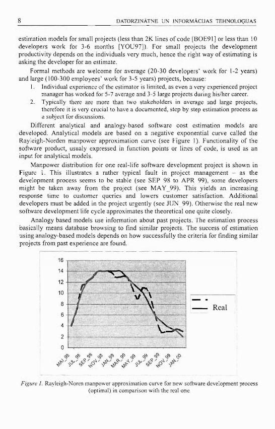
Different analytical and analogy-based software cost estimation models are developed. Analytical models are based on a negat ive exponent ia l curve called the Rayleigh-Norden manpower approximat ion curve (see Figure 1). Functionali ty of the software product, usualy expressed in function points or lines of code, is used as an input for analytical models .

Manpower distribution for one real-life software deve lopment project is shown in Figure 1. This illustrates a rather typical fault in project management - as the deve lopment process seems to be stable (see S E P _ 9 8 to A P R _ 9 9 ) , some developers might be taken away from the project (see M A Y _ 9 9 ) . This yields an increasing response time to cus tomer queries and lowers cus tomer satisfaction. Addit ional developers must be added in the project urgently (see J U N _ 9 9 ) . Otherwise the real new software deve lopment life cycle approximates the theoretical one quite closely.

Analogy based models use information about past projects . The est imation process basically means database b rows ing to find similar projects. The success of est imation using analogy-based models depends on h o w successfully the criteria for finding s imilar projects from past experience are found.

Figure 1. Rayleigh-Noren manpower approximation curve for new software development process (optimal) in comparison with the real one

Bciiha Apine. S o f t w a r e D e v e l o p m e n t Effort E s t i m a t i o n 9

Samples of Analytical Models

SLIM (Software Lifecycle Model) was developed in the middle of the 1970's [K.EM87] and currently is maintained by Q S M (Quanti tat ive Software Management ) [QSM02] . The Model was developed using data about 5000 software development projects. The SLIM model uses a productivity parameter and productivity index, which characterise the deve lopment environment (tools used, developers ' skills etc.). In compar ison to other analytical models , in the SLIM model a schedule must be set before the effort is est imated. However this is not a disadvantage of the model, because in real life very often the schedule is already predefined.

The Jensen model [JEN84] est imates the deve lopment effort and schedule based on the size of the product , technology index and 11 deve lopment envi ronment factors, which characterize the development technology. A Current version of the Jensen model is implemented in the tool S A G E [JEN95] .

C O C O M O II [COC2] estimates the development effort and schedule based on the size of the product, 5 scaling drivers and 6 adjustment factors, which describe the product 's quality and reliability requirements , technologies used, developers ' skills etc

At the end of last year a survey about the most popular deve lopment effort est imation method was carried out by [ISB01] in more than 100 software development organizat ions of varied sizes [ C L T 0 3 ] . More than a quarter of the respondents (27%) use various analytical models . A surprisingly low number (9%) report the use of C O C O M O , which was considered by many to be a groundbreaking technique in the 1980s. O n e possible explanation for this is that the C O C O M O applications are often cumber some and require the use of other tools and techniques to generate input to C O C O M O , such as lines of code est imators.

Samples of Analogy Based Models

The Checkpoint model is based on information about 8000 software development projects. This model is property of SPR (Software Productivity Research) [ JON96] . The Checkpoint model uses a survey containing mult iple-choice quest ions about the deve lopment process and the product must be developed. Information from the survey then is used to adjust the productivity of the development process.

The same principle as for the Checkpoint model is used in the Exper iencePro model and tool, which is property of Software Technology the Transfer [EXP02] . This model uses information about approximately 500 past projects. All the users of this model arc jo ined in F i S M A [FIS03] and encouraged to collect information about projects to update the Exper iencePro model continously.

Accord ing to the survey by [ ISB01] , most organizat ions (65%) collect historical data and use it to help them estimate software development . 2 6 % report that they do so diligently, by maintaining a central database that formally receives and stores data from every project.

10 D A T O R Z I N A T N E U N I N F O R M A C I J A S T E H N O L O G I J A S

Conclusions

Analytical models as well as analogy based ones use data about the software development process (measurements ) , consider different risks and their influence on the development process. A Set of risks is predefined and depends on the model. Table 1 shows software deve lopment risks found out in the survey of risk management [API02] . There are risks which are considered in each cost es t imat ion model , for instance, an unrealistic project schedule and budget or lack of knowledge in software development technologies and envi ronment . At the same t ime there are r isks which are important and influence the development schedule and effort, but are not considered by any of the estimation models analysed. For instance, software deve lopmen t environment bugs or change of qualified personnel .

Table 1. Risks considered in different software cost estimation models (+ - the model

considers that)

Software development influencing factor

C/)

S.

Che

ckpo

int

'-> '_j

53 •j

2 3

3 3

Lack of hardware on the customer side

Difficult communication with customer -Low quality of software requirements - - -Unstable software requirements - -L'nrealistic schedules and budgets - - -Weak project management - -Software development environment buss Lack of developer motivation -Lack of hardware on developers side - -Change of qualified personnel Lack of knowledge in software development technologies and environment

- - - -

Models concentrate on effort and schedule es t imat ion for new software development [ P L T 9 2 ] , [ JEN84] , [ JON96] , [ C O C 2 ] . [ E X P 0 2 ] , [PAR95] , [TAU81] . There are add-ons deve loped for some models to apply them to more specific projects like software main tenance [COC2] , [EXP02] . Tak ing into account that models rely on development process measurements , they are becoming out-of-date continuously as technologies develop. For instance, software deve lopmen t productivity increases by 10% annually. Hence using a year old cost es t imat ion mode l , it overest imates the effort by 10% even if we exactly how know to use the model . To solve this problem, authors continuously gather data about projects to mainta in their mode ls [QSM02] , [JON96] . This problem could not be solved for analytical mode l s , but for analogy based ones it is not so actual if the project base is updated with information about new projects continuously, like it is done for [EXP02] .

Bulba Apine. S o f t w a r e D e v e l o p m e n t Effort EMimat ion u

There are add-ons for deve lopment process operational p lanning developed for some of the models , which are based on the Rayle igh-Norden manpower curve [PUT92] . There are no such add-ons for analogy based models , because data gathering for such models is much more complex than approximation of the development process using analytical methods . The deve lopment of such add-on requires integration of the measurement and risk managemen t processes .

What to do?

To est imate the software product development effort and schedule the following steps must be carried out.

1. Perform a risk analysis for the particular project to find out what factors will influence the development of the product.

2. Choose the development effort estimation model which takes into account all the risks pertaining to the particular project.

Such an approach is not feasible due to the following reasons: 1. There is no knowledge available about different models. Experience shows that

most companies have knowledge about one or two effort estimation models. 2. Application of most of the models requires acquisition of specific, rather expensive

tools (several thousand EUR for licence and approximately a thousand EUR for annual maintenance of the model).

Therefore one formal model must be chosen for usage in the company . There are some sources which reccomend usage of two formal models for est imation in parallel [ ISB01] , [ JON96] . The second model is to verify the results given by the first one. Instead of the second formal model , development process measurements could be applied to adjust the formal results. Developers and managers must be trained to use the chosen formal model to avoid painful estimation mistakes.

The development process must be measured in order to use the gathered information for analysis of the results obtained from application of the formal model. Results must be communica ted a m o n g the developers.

References

[EXP02] "Estimation and Measurement Methodology of Experience Pro 3.0". [Electronical resource].-Access: WWW. URL: http^Avww.sttffi/html.-Resource described 12th of June, 2002.

[COC2] C.Abts, B.Boehm, B.Clark. S.Devnani-Chulani. "COCOMO II Model Definition Manual". University of Southern California, 2000, 68 p.

[KEM93]Chris F. Kemerer. "Empirical studies of assumptions that underlie software cost estimation". Information and Softw. Techno!., Vol.34 =4, 1992, pp. 21 1-218

[BOE91] Barry-' W. Boehm. "Software Risk Management: Principles and Practices". IEEE Software, January, 1991, pp. 32-41.

•YOU97] Yourdon. E. "Death March. The complete Software Developer's Guide to Surviving 'Mission Impossible' Projects". Prentice Hall, 1997. 2 I 8 p.

[K.EM87] Chris F. Kemerer. "An Empirical Validation of Software Cost Estimation". ACM Communication. May, 1987. pp. 416-429

12 D A T O R Z I N A T N E U N I N F O R M A C I J A S T E H N O L O G I J A S

[QSM02] "SLIM-Estimate 5.0". [Electronical resource].-Access: WWW. URL: http:/ 'www.qsm.com-'slim estimate.html.-Resource described 3rd of January, 2003.

[JENS4] Randall W.Jensen. "A Comparision of the Jensen and COCOMO Schedule and Cost Estimation Model". Proceedings of the International Society of Parametric Analysis, 1984, pp. 96-106.

[JEN95] Randall W.Jensen. "A New Perspective in Software Schedule and Cost Estimation". [Electronical resource].-Access: WWW. URL: http://www.seisage.com.'publications.htm -Resource described: 17th of February, 2003.

[ISB01] International Software Benchmarking Standards Group. "Practical Project Estimation" 2001. 46 p.

[CUT03] "The Guru Method Prevails". [Electronical resource].-Access: WWW. URL: http:/'www.cutter.com 'benchmark, index.html.-Resource described 12th of February. 2003.

[JON96] Caper Jones. "Applied Software Metrics". McGraw Hill, 1996, 324 p. [F1S03]"Finnish Software Metrics Association". [Electronical resource],-Access: WWW. URL:

http:/Avww.fisma-network.org.-Resource described 12th of February, 2003. [API02] Baiba Apine. "Software Development Risk Management Survey", accepted paper for

I 1th International Conference on Information Systems Development, Riga. Latvia. September 12 - 14, 2002. http://www.cs.rtu.Ivisd2002 accepted.asp.-Resource described:2003.g. 3.jan.

[PUT92] Lawrence H. Putnam, Ware Myers. "Measures for Excellence". Yourdon Press Computing Series, 1992

TAR95] Naval Sea Systems Command . "Parametric Cost Estimating Handbook". [Electronical resource].-Access: WWW. URL: http:,Vw~ww.jsc.nasa.gov/bu2/PCEHHTML/pceh.htm.-Resource described: 2003. g. 17.fob.

[TAUSI] Robert C. Tausworthe. "Deep Space Network Software^Cost Estimation Model". Jet Propulsion Laboratory Publication 8 1-7. Pasadena. C.A., April, 1981

L A T V I J A S U N I V E R S I T A T E S K A K S T I . 2 0 0 4 . 6 6 9 . s g . : D A T O R Z I N A T N E I ' N I N F O R M A C I J A S : : . i : \ o i . o i i . : . \ s . 13.-33. [pp.

Description of Semantics and Code Generation Possibilities for a Multi-Language Interpreter

Guntis Arnicans Faculty o f Physics and Mathemat ics . Universi ty of Latvia Raina Blvd. 19. Riga LV-1586 . Latvia, garnican@lanet . lv

In this paper we describe the definition of semantics for a Multi-Language interpreter (MLI), which provides the execution of the given program, receiving and exploiting corresponding language syntax and the desired semantics. We analyze the simplest solution the MLI receives the language syntax and the semantics descriptions, which have already been compiled to executable objects. Semantics is defined as a composition from several semantic aspects, considering the pragmatics of a language. Semantic aspects are translated to semantic functions by composing descnptions of the aspects. A traversing program's intermediate representation and the calling out of semantic functions similarly to the principle of the Visitor pattern perfonn the desired semantics. To simplify the semantic descriptions, we use abstract components that are joined by connectors at the meta-levcl. The implementation of these components and connectors can be very different. Examples of conventional and specific semantics are given for the simple imperative language in tins paper. Key words: interpreter, programming language specifications, tool generation.

1. Introduction

T h e number of new languages that are related to the IT sector has increased rapidly over t he last several years (p rogramming languages and data description languages , for example) . Problems associated with the implementat ion and use of these languages has also expanded, of course . Kinnersley [Kin95] has reported that there were 2,00(1 languages in 1995. which were being put to ser ious use. Even back then specialists found that the new languages were most ly to be classified as domain-specific languages. Most o f them are not easy to implement and maintain [ ITSE99, DKVOO (DSL analysis, p roblems and an annotated b ib l iography)] . It is also true that we need not jus t a compi le r or an interpreter, but also a number of support ive tools. Quest ions of p rogramming quality a re very important today, and these questions often cannot be answered without specialized and automated ancillary resources.

Computers are be ing used with increasing dynamism today: systems have been divided up in terms o f time and space, the operational envi ronment is heterogeneous , and w e have to ensure the implementat ion of parallel processes whi le organizing cooperation among componen t s and systems, adapt ing to changing circumstances wi thout interrupting our work. etc. We are making increasing use of interpreters or of code generat ion and compila t ion just in time. The formal resources that are used to descr ibe the semant ics of a language, however, cannot fully satisfy our needs in the modern age, and they a re starting to lose their posi t ions [Sch97, Lou97, Paa95] ,

T h e basic problem that is associated with the formal specifications of programming languages is that these specifications are far too complex . It is not clear how they are administered, w e cannot use them to explain all of our practical needs, and in the end we are still faced with a problem - who can prove that these complex specifications are really correct? The literature c la ims that the best commerc ia l compilers (interpreters or other language-based tools) are written without formalism or are used only in the first

14 D A T O R Z I N A T N E L'N I N F O R M A C I J A S T E H N O L O G I J A S

phases - scanning and parsing [e.g. Lou97] . Formal i sms are elaborated and used mostly for research purposes in educational and scientific insti tutions at this time.

The development of semant ics is gradual ly moving away from the deve lopment of languages and tools. One way to overcome this gap is to take a tool-oriented approach to semantics , making the definitions of semant ics far more useful and product ive in practice and generat ing as many language-based tools as possible from them [HKOO]. We support this approach in principle, but our aim is to propose a different approach toward the definition of semant ics , making r o o m for far less formal records.

Those w h o prepared descriptions of semant ics in the past have long since been looking for ways in which semantics can be divided up into reusable components , and it is not yet clear whether the formal or the partly formal methodology is the best in this case. We chose a less formal and more free form of descript ion keeping from the theoretical perspect ive, and our empirical research showed that rank-and-file developers of tools understand this method far more easily.

2. The concept of a Multi-Language Interpreter

The concept of a mult i - language interpreter was in t roduced in [AAB96] . A Multi-Language Interpreter (MLI) is a program which receives source language syntax, source language semant ics and a program writ ten in the source language, then performs the operations on the basis of the program and the relevant semant ics . Conceptual ly , we parse an input token stream, build a parse tree and then t raverse the tree as needed so as to evaluate the semantic functions that are associated with the parse tree nodes. Once an explicit parse tree is avai lable, we visit the nodes in some order and call out an appropriate function. This approach is similar to the pr inciple build a tree, save a parse and traverse it [Cla99] and to a Visitor pat tern [ G H J V 9 5 ] , except in terms of the methodology which we apply in obtaining semant ic functions and organizing physical implementat ion. The idea of MLI is expressed in Figure 1.

Syntax

Seman t i cs Mu l t i - l anguage nterpreter

P r o g r a m

- / Results

Figure I. The concept of a Multi-Language Interpreter

The concept of a MLI presupposes that we can prepare several semantics for one syntax, and we can exploit one semantic for var ious syntaxes . The descript ions of syntaxes and semantics must be translated to the executable form (before or during the running of the MLI) . MLI implementat ion archi tectures may vary. The one we use receives and exploits syntax and semantic descr ipt ions that have already been compiled as executable objects (Figure 2). Syntax is represented by the SyntaxObject , and semantics by the TraverserObject . the Semant icObjec t . the SymbolTable . and the necessary volume of the Component (the componen t s A, B. C in our figure). T h e MLI Kernel , which provides the initial bonding of all syntax and semantics objects, initializes the execution of the program.

Gitntis Amicans. D e s c r i p t i o n of S e m a n t i c s a n d C o d e G e n e r a t i o n Poss ib i l i t i e s 15

Results

Figure 2. MLI runtime architeeture

Each of the componen t s can be implemented in various ways - with a different semantic ass ignment and physical implementat ion. Here we have a chance to combine syntaxes and semant ics in both ways - in terms of architecture and in terms of implementat ion. Then, however , we immediately face the question of the compatibili ty of the syntax and semant ics so as to avoid senseless interpretation.

The obtaining of an executable syntax and of semantic objects from their descriptions can be done before or during the actual program execution (analogue to a classical compiler and interpreter). Dynamic code generat ion is more difficult because all generation phases mus t be done automatically.

3 . Language Specifications for MLI

Programming language is an artificial means to communica te with a computer and to fix the a lgori thms for problem solving. Like a natural language, a programming language ' s definition consists of three components or aspects: syntax, semantics and pragmatics [Pag81 , S K 9 5 ] , All of these aspects are significant in deal ing with our problems. Usually exploi ted rarely, pragmatics deals with the practical use of a language, and this is an important e lement in defining semant ics .

We can look at syntax and semant ics from two perspect ives - the definition or description phase and the runtime phase. Our goal is to achieve runt ime components which can freely be exchanged or mixed together in pursuit of the desired collaboration. First we must look at the principles of syntax and semant ics descript ions, and then we can view the target code generation steps.

Our basic principle is to divide syntax and semant ics into small parts, and later, with a simple method , to combine these parts thus providing a mechanism to tie together the semantic parts and the syntax elements. Our method is close to some of the structuring paradigms o f attribute grammars [Paa95]: The definition phase is similar to the relat ionship Semant ic aspect = Module , but the runt ime phase is similar to Nonterminal = P rocedure . That means that we basical ly use the language pragmatics and divide the semant ics into semantic aspects.

3.1. Syntax

The formalisms for dealing with the syntax aspect of a p rogramming language are well developed. The theory of scanning, parsing and attribute analysis provides not only the means to perform syntactical analysis, but also a way to generate a whole compiler as well. Such terms, concepts or tools as finite automata , regular expression, context-free grammar , at t r ibute g rammar (AG), Backus-Naur form (BN'F). extended BNF

16 D A T O R Z I N A T N E E N I N F O R M A C I J A S T E H N O L O G I J A S

(EBNF) , Lex (also Flex). Yacc (also Bison) , and P C C T S are well known and accepted by the computer science communi ty .

We do not need to reinvent the wheel and it is reasonable to choose the existing formalisms and generators ( lexers and parsers) . The main task when deal ing with syntax description for a given language is code genera t ing which can transform the written program, which uses the syntax, into in termediate representat ion (IR). Addi t ional ly , we need to attach a library with functions, which provide the means to manipula te with the IR and to compi le the whole code. The result is the SyntaxObject (Figure 2).

In this paper we concentrate most ly on the class of imperative programming languages, but our method is adaptable for other languages too , such as d iagrammat ic languages (e.g., Petri nets. E-R d iagrams , Statechar ts . V P L - visual p rogramming languages, etc.). which exploit other formal isms (e.g., SR G r a m m a r s . Reserved Graph Grammar) and processing styles [FNT-i-97, ZZ97] ,

3.2. Semantics

The chosen principle for the runt ime semant ics parse and traverse states that the most important things are a t raversing s t ra tegy and the semant ic functions which must be executed when visiting a node (Figure J ) . Therefore, the central componen t s of the semantics are TraversalObject and Semant icObjec t (Figure 2).

The TraversalObject manages the node visit ing order, provides semantic functions with information from the IR, and is the main engine of the MLI . The SemanticObject , for its part, contains all of the necessary semant ic functions and provides for the execution environment . At the same t ime, w e can also put into the semantic functions certain commands which force the Traverser to search for the needed node and to change the current execut ion point in the IR ( traversing strategy changes and a transition to another node are problems in the Visitor pattern [e.g. VisOl]) .

Semantic functions have to be as s imple and as small as possible. This can be achieved by using a meta- language and by employ ing high-level expression means , which allow for easy unders tanding and verification of the description. Fol lowing this

Gunris Arnicans. I n s c r i p t i o n of S e m a n t i c s a n d C o d e G e n e r a t i o n Poss ib i l i t i e s 17

principle becomes more natural if we use abstract components so that the underlying semantic can be clear without addit ional explanat ions (in Figure 3, the abstract components already have a concrete implementat ion component - A, B and C). This s tatement may lead to objections from the advocates of formal semantics , because the components are not described with mathemat ic precision. At the same t ime, however , formal semantics somet imes use such concepts as Stack or Symbol table.

Let us introduce a conceptual syntax element, which is a g rammar symbol with a name (e.g., a named nonterminal symbol or a named terminal symbol) . Consider ing the various types of syntax elements and the traversing strategy, we separate various visitations and introduce the concept of the traversing aspect. For instance, we can distinguish the arriving into node from the parent node (PreVisit) as well the arriving into node from the child node (PostVisi t) . Thus we create the semantic functions and name them not only on the basis of the n a m e of the syntax element but also on the basis of the arriving aspect ( traversing aspect) into this e lement (Figure 3).

Runt ime semantics or simply semant ics for mult i - language interpreters are a set of semantic functions. W e represent the runtime semant ic in Table 1. There is an executable code ( c ) or nothing (A.) for the syntax e lement , according to the traversing aspect, n depends on the size of syntax (e.g.. the count of all nonterminal and terminal symbols ) , and m depends on the complexi ty of the t ravers ing strategy (usually 1..3). We notice that the matrix mainly consists of empty functions (X.).

Tabic 1. The matrix of syntax elements and semantic function correspondence

Syntax Element (SE)

Traversing Aspect (TA) Syntax Element (SE) T

A, T

A-, T

A-, T

SE, - X X

S E : X X A

SE, X X X

A SE„ • X K X

The identification of semantic functions is realized both by the syntax name and by the traversing aspect name . Technical implementat ion may differ, but it is very advisable that functions identification and call ing be performed with constant complexi ty 0 ( 1 ) .

N o w we arrive at the most difficult and important problem - how can we obtain semantic functions and ensure correct collaboration be tween them, and how is it possible to create reusable semantic descriptions? Let us explain our ideas about how to define semantics and h o w to gain the matrix observed above, i.e.. how to generate executable semantics from the semantic description.

18 D A T O R Z I N A T N E U N I N F O R M A C I J A S T E H N O L O G I J A S

4. Semantic Aspects and Abstract Components

4.1. Semantic aspects

In practice, p rogramming languages are frequently presented through the pragmatics of the programming language, i.e.. examples are used to show how the language constructs are exploited and what their under ly ing meaning is. Let us call these language constructs and their meaning like semant ic aspects .

We have chosen to define the semant ic as a set of mutual ly connected semantic aspects. Here are some examples for typical groups of semant ic aspects for imperative p rogramming languages: execution of c o m m a n d s or s ta tements (e.g., basic operat ions, variable declaring, assigning of a value to the variable, execut ion of ari thmetic expressions) , program control flow managemen t (e.g., loop with a counter, conditional loop, condit ional branching) , dealing with symbols (e.g., variables, constants) , environment management (e.g.. the scopes of visibili ty). Here, too. are examples of nontraditional semantic aspects: attractive print ing of the p rogram, dynamic accounting of statistics, symbolic execution, specific p rogram inst rumentat ion, etc.

We have chosen an operational approach to descr ibe the semantic aspect - we define the computat ions , which a computer has to do to perform the semantic action.

4.2. Abstract data types and abstract components

The next significant principle to define the semant ic aspect is using abstract data types (ADT) as much as possible. A D T is a collect ion of data type and value definitions and operat ions on those definitions, which behave as a primitive data type. This software design approach breaks down the problem into componen t s by identifying the public interface and the private implementa t ion .

In our case, typical examples of A D T are Stack. Queue , Dict ionary, and Symbol table (in compiler construction theory [ASL'86, FL88] , in formal semantics [SK95]) . In this way we hide most of the implementa t ion details and concentrate mainly on the logic of the semantic aspect. Later we can choose the best implementat ion of A D T for the given task. Seeing that some exploi ted componen t s can be complicated (E-mail . Graph visualization. Distributed communica t ion , Transac t ion manager , etc.) and have no s tandards, we use another term - abstract componen t . Somet imes we want to utilize an already existing component , and the term abstract component seems more appropriate to us.

It is advisable to describe the semant ic aspect through meta- language, even if one does not have a translator for this. Then one can translate or simply rewrite it by hand to the target p rogramming language, select appropr ia te implementat ion for the abstract components , and use the needed interface, col laborat ing protocol and execution environment . For instance. Stack can be implemented in a cont iguous memory or in a linked memory . Symbol table - as a list or as a dict ionary with the hashing technique. Fur thermore, instances of abstract componen t s can be viewed as distributed objects in a heterogeneous comput ing network.

Gunlis Arnicans. D e s c r i p t i o n ot S e m a n t i c s and C o d e G e n e r a t i o n Poss ib i l i t i es 19

4.3. Examples of abstract components

Some abstract componen t s and their operations are very popular , e.g.. Stack (createStack. push, p o p , top. etc.). Queue (crea teQueue, enqueue, dequeue, first, etc.), while some are guessed, e.g.. E-mail (prepare, send, receive, open). A m o n g the many specific componen t s we would like to emphasize one that is useful for most of semantics - Symbol table (SymbolTable in Figure 2) or its analogue to provide the execution environment .

While building prototypes of the MLI . we have created an implementat ion of Symbol table - M O M S (Memory Object Management Sys tem) - that is appropriate for implement ing the imperat ive programming languages. It is possible to define basic and user defined data types , to define base operations and functions, to operate with variables and their va lues , to manage the scope of visibility of all objects, etc. The most important data types, concepts , and operations of M O M S are listed in the appendix to this paper so as to give the reader a better idea about M O M S .

The second important component is Traverser (TraverserObjeet in Figure 2). Its main task is realizing the traversing strategy, to change the current execution point and to organize cooperat ion with the syntax object.

There is a depth-first left-to-right traversing strategy, which is used in the following examples (Table 2) . This strategy has three visiting aspects : Visit (for tree leaves -terminals) , PreVisit and PostVisit (for the other tree nodes - nonterminals) . To define semantic functions for examples , we have used the fol lowing operat ions: NodeValue() returns a value for the current terminal or nonterminal symbol (value from the current IR node) , and both goSib lForw(aName) and goS ib lBackw(aName) provide for a changing of the current node , searching the node with the n a m e aName between siblings going forward or backward .

Table 2. A depth-first left-to-right traversing strategy

Travcrse(nodc P) if IsLeaf(P)

Visit{V) PreVisiiy?) for each child Q of P. in order, do

Traverse! 0 ) PostVisit(P)

It is possible to describe interfaces for SyntaxObjec t . TraverserObject and Semant icObject with domain-specific language. Then interfaces for obtaining the IR. manipulat ing with it and working with the symbol table can be compiled together, and it is possible to engage in high-level optimization and verification [Eng99] ,

The Travers ing strategy can also be described with domain-specific language. This is important if the strategy is not trivial and depends on syntax elements and the program state [ O W 9 9 (traversing problems and solut ions for Visitor pattern)]. The traversal strategy should be independent from syntax as much as possible and organized

20 D A T O R Z I N A T N E UN I N F O R M A C I J A S T E H N O L O G I J A S

(combined) by patterns [VisOl] . In addit ion to c o m m o n t ravers ing strategies there are also less traditional ones , e.g., the strategy for reverse execut ion of the p rogram [BM99]

4.4. Defining the semantic aspect

It is more convenient to define the semant ic aspect by using d iagrams (as in Figure 7). W e can write a meta -p rogram or a p rogram in the target language in textual form, too. Diagrams contain syntax e lements that are important for the semant ic aspect and are visualized with graphic symbols . W e can use different graphic notat ions. If the visiting order of syntax e lements is important , then we mark the order with arrows.

Let us call the operat ions that are performed dur ing the aspect node visiting semantic action. Semant ic action is s imi lar to semant ic function, but it is written at the meta-level and relates only to a given semant ic aspect. Semant ic action is shown as a box with the meta-code connected to the syntax e lement and takes into account the traversing aspect.

There are all kinds of abstract data types that are needed for the semantic aspect into the box with the key words I M P O R T G L O B A L . For better perceptibil i ty of the semantic aspect, it is permiss ib le to use addit ional graphic symbols that are not needed in real execution. For instance, we use Other aspects to signal that we expect there to be a composi t ion with the other semant ic aspects .

4.5. Examples of semantic aspects

Let us look at s o m e examples of semant ic aspects (Figure 4 - Figure 8) that are applicable for the s imple imperat ive p r o g r a m m i n g language Pam [Pag81] . Terminal symbols are denoted by a rectangle , while nonterminal symbols are indicated by rounded rectangles. T h e left circle in the nontermina ls corresponds to the PreVisit semantic action, the right one - to the PostVisi t semantic action, while for the terminals, the Visit semantic action is assigned.

IMPORT GLOBAL Env of AD7_8 y T r i b o 1 Tab 1 e

L-OGE.-.V () ^ J0 p r o g r a m Gj

C_Other a s p e c t s ~'

ENV. releas«?rogtr.v ()

Figure 4. The semantic aspect PROGRAM. It prepares the program environment to manage variables, constants, etc. and operations involving them. The environment is destroyed at the end

IMPORT GLOBAL CanCreateVar of Stack ! /r-

1 (G va r i ab le_de f (Tj)

CanCreateVar. ir .Crea t ieV'ar . p e p () '„ O t h e r a s p e c t s _ J

Figure 5. The semantic aspect VARIABLE DEFINITION. It allows for variable creation

Gumis Amicans. D e s c r i p t i o n of S e m a n t i c s a n d C o d e G e n e r a t i o n Poss ib i l i t i e s 21

IMPOST GLOBAL Trav cf ATTJTreeTraverser, ?efStack of ADT Stack, Er.v of ADT SymbolTabie, CanCreateVar of ADT Stack

LOCAL VarT-xt = Trav. oodeValue () if CanCreateVar.top() - TRCE and

Env.flftdvar(Vertex t) = FALSE Env.createVar(VarTe xt, INT)

endif LOCAL ?.ef = Env.getRe f VarText) RefStack.p-jsh (Ref)

LOCAL IntText = Trav.nodeValue() LOCAL Ref = Env.getRef ( " TNT_" + lntTe>:t! If Ref = EMPTY

LOCAL Integer = TextToInteger (IntText) Ref = Er.v.createLitJ" INT_"»rr.t>.xt, :XT; Env.p'utValue (Ref, Ir.teger)

endr f RefStack.push(Ref i

Figure 6. The semantic aspect ELEMENT. It provides for the pushing into the stack all references to each variable encountered while traversing. Variable creation is forbidden by default. The Trav

provides for getting the values of the current terminal node in IR.

IMPORT GLOBAL RefStack of AST Stack, Snv of ADT SymbolTabie

LOCAL Res = RefStack.pop() LOCAL Var = Ref S tac•:. pop () LOCAL Vol = Env.getValue(Pes) Er-.v. p-JtValue (Var, Val)

(O a s s i g n m e n t _ s t a t e m e n t ( 7 - H

I " t (O ! e f t _ h a n d „ s i d e Q)—>- ASSIGN —>{Q r i g h t _ h a n d _ s i d e

Y X \ t 1

' ' O t h e r a s p e c t s ~> \ 'T_Other a s p e c t s / , 1

5

Re fStack.push(NULL) Ref Stack, pcsh (NULL)

Figure 7. The semantic aspect ASSIGNMENT. It takes reference to the variable and reference to the value from the stack and assigns a value to the variable. Pushing of references is simulated

22 D A T O R Z I N A T N E I N I N F O R M A C I J A S T E H N O L O G I J A S

IMPORT GLOBAL RefSrack, Sort, Flag of ADT_5tack, Trav of ADT TreeTraverser, Env of ADT SyrtbolTable

W H I L E - * { / c o m p a r i s o n C ^ — > ~ D O —>-(C s e r i e s J)—>- END

Othe r a s p e c t s

if Sort, top () = INDEF t h e n LOCAL Ref = RefStack.popO if Er.v.getValue(Ref) - FALSE

Flag.replaceTop(FALSE! Trav.goSibiForw(@END)

e n d if endif

Ref Stack, push (NULL)

if Sort.topO = INDEF and Flag, top () - TRUE

Trav.goSiblBackw(@WHILE) endif

Figure <H. The semantic aspect INDEFINITE LOOP. It "goes through"' the series and back to WHILE until the comparison sets a NL'LL reference or a reference with the value FALSE

5. Meta-semantics

Meta-semant ics is a term which relates to a meta -nrogram that describes the counterparts of which semantics consists and the way in which these counterpar ts are connected together. The conceptual s cheme of meta-semant ics is shown in Figure 9.

Nonterminals S y n t a x Terminals

Figure 9. The conceptual scheme of meta-semantics. For instance. SA1 involves nonterminal NT I and terminal T l , and SCI is performed while prcvisiting. SCI is a composition

of ISA I and ISA4

(funtis Arnicans. D e s c r i p t i o n of S e m a n t i c s a n d C o d e G e n e r a t i o n Poss ib i l i l i c s 23

If we look at semant ics from the definition side (the logical view) then semantics is Conned by traversing strategy and by a set of semantic aspects that consist of semantic actions realized while visiting the appropriate node of the intermediate representation. If we look at semant ics from the runtime side (the physical view) then while visiting one node it is possible that several semantic actions have to be realized, and we have to ensure correct collaboration between all involved instances of abstract components into the desired envi ronment . How can we put all of tins together correctly'?

To solve this p rob lem we introduce the concept of the semantic connector . This concept has been adapted from the concept Grey-box connector , which solves a similar problem: how to connect the pre-buiit components in a distributed and heterogeneous environment for col laborat ing work [AGBOO]. The Grey-box connector is a rricta-program that introduces a concrete communica t ions connection into a set of components , i.e., it generates the adaptat ion and communica t ions glue code for a specific connect ion.

6. From semantic aspects to meta-semantics and executable semantics

The obtaining of semantics for the fixed syntax is achieved in several steps: 1) select predefined semant ic aspects or define new ones i'or the desired semant ics , 2) rename syntax e lements and traversing aspect in the selected semantic aspects with names from fixed syntax and traversing strategy. 3) rename instances of abstract components to organize collaboration between semant ic aspects . 4) make composit ion from semant ic aspects . 5) specify the runt ime envi ronment and translate the mcta-code to the code of the target programming language, and 6) compile the semantics .

• Selection of semant ic aspects (step 1)

If we have a l ibrary with previously created semantic aspects, then we can search for appropria te ones . i.e. reuse some parts of the semant ics . The traversing strategy also has to be considered.

• Syntax e lement and traversing aspect renaming in semantic aspects (step 2)

Actually this is semantic action mapping . Matching to the fixed syntax elements is achieved by mapping syntax elements of semantic aspects to fixed syntax elements ( rename with - s imple mapping and duplicate to - mapp ing of a semantic aspect syntax element to several fixed syntax elements):

r e n a m e < n a m e > < t r a v c r s i n g a s p e c ! > with t a r g e t n a m e • < t a r g c t t r a v e r s i n g aspect-

d u p l i c a t e < n a m e > < t r a v o r s i n g aspect ' to

<targct n a m c > <target v i s i t i n g a s p c e t > [,<targct namc> • ' t a r g e t v i s i t i n g aspect> ...j

For instance, r ename left hand side PostVisit with V A R I A B L E Visit ; d u p l i c a t e C O L ' N ' T A B L F . N O D E Vis i t to V A R I A B L E V i s i t . : i s s i g n m c n t _ s t a t e m e n t P n s l Y L i t

• Renaming of instances of abstract components (s tep 3)

Match ing of componen t s is necessary-' because there is no direct data exchange between semantic functions, and we need collaborative work. The program slate is fixed by using the runtime states of components . At first we decide what instances they have

24 D A T O R Z I N A T N E UN I N F O R M A C I J A S T E H N O L O G I J A S

in common and what names they have to get, and then we rename instances in the semantic aspects:

replace <name> with <target namc>

For instance, replace RefStack with DataStack ; replace Sort with LoopSortStack

• Composi t ion of semant ic aspects (step 4)

The goal of a semant ic aspect composi t ion is to bring together several semantic aspects into one more compl ica ted aspect that nearly descr ibes entire semantics . While compos ing , we stick together the meta -code of semant ic act ions that have the same name. The sticking principles can vary, for instance, sequent ia l (one code is appended to the other one) , parallel (codes can be executed s imul taneously or sequential ly in any order) , free (the user can modify the code union as he l ikes). To achieve better results, we ignore some semantic act ions or apply the sticking principle to the semantic aspects in the reverse order. At this t ime we have to be aware of conflicts between local variable names.

compose aspect « n c w S A » (<refmed SA>) [[append ; parallel, free] (<refined SA>) . . . ] , where

<refined SA> = « o l d S A » [ignore <name> <trav aspcct> [,<name> <trav aspect>]] I [reverse]

The result is meta-semant ics . An example of a meta -code fragment for meta-semantics is given in Table 3.

Gunlis Arnicans. D e s c r i p t i o n of S e m a n t i c s and C o d e G e n e r a t i o n Poss ib i l i t i e s 25

Table 3. An example of meta-semantics

compatible with ir_type P a r s e T r e e t r a v e r s e r _ t y p e P a r s e T r e e T r a v e r s e r

syntax e l e m e n t s (prograrr., e x p r e s s i o n , V A R I A B L E , ...) semantic a c t i o n s (<PROGRAM> program i E K V . p r e p a r e P r c g E n v ( )

< ? R O G R A K > p r o g r a m PostVisit

global Trav o f A D T _ T r e e T r a v e r s e r global Env of ADT_Syrr.bclTabie create D a t a S t a c k , O p e r a t c r S t a c k , C a n C r e a t e V a r , L o o p S o r t S t a c k ,

L o c p C c u n t e r S t a c k , L c c p F i a g S t a c k , I t F l a g S t a c k cf ADT Stack create I n p u t F i l e , O u t p u t : i^e cf A D T FILE

compose aspect < A 1 > / / c o m p o s e s s e m a n t i c a spec t s from a spec t s g iven a b o v e (<PROGRAK>) /,' s e m a n t i c a s p e c t s P R O G R A M r e m a i n s the s a m e

append (<ELEMEKT> replace R e f S t a c k with D a t a S t a c k /,' r ep laces s t ack for c o l l a b o r a t i n g w o r k

rename INTEGER V i s i t with C O N S T A N T V i s i t ) // r e n a m e s n o n t e r m i n a l a c c o r d i n g to P A M syntax append (<ASSIGNMENT>

replace R e f S t a c k with D a t a S t a c k rename left h a n d side P o s t V i s i t with V A R I A B L E Visit,

right h a n d siae PostVisit with e x p r e s s i o n PostVisit ignore lef t_hand side P o s t V i s i t ) // i g n o r e p u s h i n g of N U L L re fe rence

append (<INDEFINITE LOOP> repiace R e f S t a c k with D a t a S t a c k ,

Sort with L o o p S o r t S t a c k , Flag with L o o p F i a g S t a c k ) append (<VARIA3LE D E F I N I T I O N S

rename v a r i a b l e _ d e f FreVisit with assign s t a t e m e n t P r e V i s i t , v a r i a b l e def PostVisit with ASSIGN Visit)

end compose aspect

compose aspect < A 2 > (<A1>

ignore e x p r e s s i o n PostVisit, coxpari append ( . . . /* Others a s p e c t are a p p e n d e d so

<INPUT>, < O U T ? L T > , <BAS5 3YNARY 0 C O N D I T I O N A L S T A T E K E N T > */

. . . ) end ccivpose aspect

• Meta-code translat ing (step 5)

Meta-code is t ransla ted to the target p rog ramming language, taking into account the target language (e.g. C + + ) , the implementat ion of abstract components (e.g. Stack in linked memory) , the operat ing system (e.g. Unix) , the communica t ions between components (e.g. C O R B A ) , MLI components type (e.g. DLL) , etc. The translation may be done by hand or automatical ly (desirable in c o m m o n cases).

PreVisit

. . . )

sicn FcstVisit;

oh as <TY?E AND OPERATOR>, FERATION>, <DEF:N;TE LOOF>,

26 I) A T O R Z I N A T N F: U N I N F O R M A C I J A S T E H N O L O G I J A S

• Obtaining semantic objects (step 6)

By compil ing the code we get executable objects that provide semantic performance, i.e. they contain the semant ic functions that are called whi le traversing the program intermediate representat ion. The instances of the concrete implementat ion of abstract components are created, or the exist ing ones are dynamica l ly linked via the selected communicat ions protocols.

7. Examples of alternative semantic aspects

In this section we provide a short insight on how w e can build nontraditional semantics . By adding new features to exis t ing semant ics we can create a specific tool that works with a given p rog ramming language. W e would like briefly to survey two examples : 1) statistics account ing of p rogram point visi t ing, and 2) storing of symbolic values for variables. Both aspects are added to the convent ional semant ics , and this is program instrumentation if we speak in te rms of software testing.

7.2. Accounting of program point visiting

Our goal is to account for any visit ing of a desirable p rogram point. This means that we need to set counters at these points . At first we write the semant ic aspect N O D E C O U N T E R (Figure 10). W e use the abstract componen t Dict ionary where we can store, read and update records in form <key, value>.

IMPORT GLOBAL Trav of ADT_TreeTraverser, Diet ci ADT_DicLionary

C O U N T A B L E N O D E

LOCAL key = Trov.gctNodcTDI: LOCAL reco-U = Diet.gecRecNom(key) if record = 0

Diet.createRec(key, 1) else

Diet.updat8(ro:crd, Diet.cot(record) - 1) endi f

Figure 10. The semantic aspect NODE COUNTER

Defining meta-semant ics . we add this semant ic aspect to the others. For instance, we define accounting for the use of any variable and ass ignment operation:

dublicate countable_node Visit to VARIABLE Visit. assignmcnt_statcraent PostVisit

Another semantic aspect can be built which accounts for every concrete variable using statistics into an addit ional dic t ionary (the variable name serves as the key). We can improve this aspect further by account ing for an aspect of variable use - defined, modified, referenced, released, etc. In the program analysis and instrumentat ion area, our approach is similar to the W y o n g system (based on the Eli compiler generation system and the A T O M program instrumentat ion sys tem) , because specific operations are attached to syntax e lements , and in this way we obtain a specific tool with additional semantics [Slo97].

Guruis Arnicctns. D e s c r i p t i o n ni S e m a n t i c s a n d C o d e G e n e r a t i o n Po%sihiliiics 27

7.2. Storing of symbolic values for variables

The second example provides for the fixing of symbolic values for variables (Figure 11). To do this task in an effective way, we have additional operat ions in our M O M S (symbol table). The operation createSymbVal t ie creates an entry for symbolic value, and with the operations addTex tToSymbValue and addVarToSymbValue , we form the value while traversing all nodes in the desired subtree (we store all needed program symbols and symbolic values of variables). At the end we store accumulated value wi th the operation s toreSymbValue .

IMPORT GLOBAL Trav o f A O T _ T r e e T r a v e r s e r H SymfcR«fSi:ack o f A D T _ s t a e k , Er.v at ACT^SymbalTahle , Car.CreateSyrr.bVar o f ACT_staclc car,Craar:eSyr.bVar . p u s n I FALSE)

LOCAL Syrr-cVar - £ y n i : P . e r S t a c k . p o p [] Env. s t o r e S y r i : V a l u e (SynbVar , S y r i V a U

ast.- • • • •en:_5 ' .a ier r ;e ' i l 2 > —

CafiCzeateSyrriVar . pop \)

l e f t h a n d Side Tu)—^\ A S S I G N n g h t _ h a n d _ s ; d e

'„ O t h e r a s p e c t : ' ^ _ 0 ' h e r a s p e c t s ^ '

? a c k , p u s r - t H U L L ) |

LOCAL S y n b T e x i » T r a v . n o d e V a l u e I } LOCAL Synfcp.ef - S y m b R e E S t a c k . t o p ( ) En v . addTeKCToSymfiValije (SymbP-ef, S y n b T e x t )

LOCAL VarTeKt =• T r a v . n o d e v a L u e < ) LOCAL Eyru'-'flcName = " SYMB_" i VarTusc: i f CanCreateSymtrt /ar . t o p l) - TRUE

1£ E i w . f Lr .dVjr(5yrnbvai7ex*0 - FALSE E n v . c r e a t e V a r (SymfcVarTexTi^ SYKSJ

e n d i f LOCAL S y n b R e : - E n v . q e t R e f (SyrctoVarTexc) Er.v. c r e a t e s y r n b v a l u e (Syrr iRe: ) SVT-bRe i S zack. p u s n IZynvt Re f )

e l s e LOCAL, SymbP.ef - Enir.getP-e f [Syirf-jVarText) Er.v . acdVarTc-SyrrJ-A'alue (SymbRef.)

er.da f

Figure 11. The semantic aspect SYMBOLIC VALUES

8. Conclusions

This method was developed with the goal of reducing the gap between practit ioners (tool developers) and theoreticians (developers of formal specifications for semantics) . Our exper ience shows that a significant achievement is attained if abstract components or abstract data types realize the greater part of semant ics , because that way it is easier to perceive the full implementat ion of semantics .

The second acquisit ion of our method involves significant disjoining of syntax and semant ics from each other. It allows us to combine various syntaxes and semantics and to find out the most desirable semantics for the given syntax. So. if we have written syntax for a new language, we can match several semant ics to it in a comparat ively short t ime. As a result, we can develop a wide spectrum of tools in support of our new language.

Our approach al lows us to change semantics dynamical ly while the interpreter is running, i.e. replace semantics or execute various ones s imultaneously. It is possible to reduce a derived parse tree (by deleting nodes with empty connectors) or to optimize it (tree restructuring statically and dynamical ly , considering performance statistics).

28 D A T O R Z I N A T N E U N I N F O R M A C I J A S T E H N O L O G I J A S

At this moment the envi ronment for tool construct ion or semant ics generat ion is not completely developed. Our experience shows that tools can be developed without significant investments , for example , by us ing L e x / Y A C C as a generator to create a syntactic object, which produces program intermediate representat ion. It is not too difficult to develop a Traverser and a s imple SymbolTab ie . A n d as the last j ob , we have to work up semantic aspects on the basis of our me thod and compose them, thus obtaining connectors , which can be written in some c o m m o n programming language (skipping meta- language use and its t ranslat ion) . The use of abstract components depends on target semant ics .

We believe that the deve lopment of the ser ious tools demands a more universal implementat ion of the Symbol table. Our Symbol table implementa t ion - M O M S - is not applicable only for imperat ive language implementa t ions . It was also the basic object-oriented database for the commerc ia l appl icat ion Mosaik (Sietec consult ing G m b H Co. O H G . graphical C A S E tool for bus iness model l ing) .

The weakness of our method lies in the semant ic aspects composi t ion stage. At this moment we have not analyzed all risks in te rms of obta in ing senseless or erroneous semantics . The problems are not trivial, and they are s imilar to problems in the proper collaboration of objects or components in object-or iented p rogramming , too. [e.g. ML98] , Most name conflicts can be prec luded automat ica l ly , but it is considerably harder to organize col laborat ion a m o n g the c o m m o n c o m p o n e n t s in semant ic aspects (it is easier if the semant ic aspects are mutual ly independent) .

Another problem is that the language g r a m m a r is frequently not context free (this is true of our example above , too). In this case we have to introduce addit ional flags to memor ize the context of syntax e lements . It is advisable to rewri te the syntax and to use context-free grammars .

9. References

[AAB96] V. Arnicane, G. Amicans, and J. Bicevskis. Multilanguage interpreter. In H.-M. Haav and B. Thalheim, editors, Proceedings of the Second International Baltic Workshop on Databases and Information Systems (DB&IS '96), Volume 2: Technology Track, pages 173-174. Tampere University of Technology Press, 1996.

[AGBOO] U. ABmann, T. GenBler, and H. Bar. Meta-programming Grey-box Connectors. Proceedings of the Technology of Object-Oriented Languages and Systems (TOOLS 33), pp.300-31 1, 2000.

[ASUS6] Alfred V. Aho, Ravi Sethi, and Jeffrey D. Ullman. Compilers: Principles, Technigucs, and Tools. Addison-Wesley, 1986.

[BM99] B. Biswas and R. Mall. Reverse Execution of Programs. ACM SIGPLAN Notices, 34(4):61-69. April 2000.

[Cla99]C. Clark. Build a Tree - Save a Parse. ACM SIGPLAN Notices, 34(4): 19-24, April 2000. [DKV00] A. Deursen. P. Klint, and J. Visser. Domain-Specific Languages: An Annotated

Bibliography. ACM SIGPLAN Notices, 35(6):26-36. June 2000. [Eng99] Dawson R. Engler. Interface Compilation: Steps toward Compiling Program Interfaces

as Languages. In DSL-99 [ITSE99], pp.387-400. [FL88] Charles X. Fisher, and Richard J. LeBlanc. Jr. Crafting A Compiler. Benjamin-

Cummings, 1988.

Guntis Amicans. D e s c r i p t i o n of S e m a n t i c s and C o d e G e n e r a t i o n Poss ib i l i t i e s 29

[FNT-97JF. Ferrucci, F. Napolitano, G. Tortora. M. Tucci, and G. Vitiello. An Interpreter for Diagrammatic Languages Based on SR Grammars. Proceedings of the 1997 IEEE Symposium on Visual Languages (VL '97), pages 292-299, 1997.

[GHJV95]E. Gamma, R. Helm, R. Johnson, and J. Vlisides. Design Patterns: Elements of Reusable Software, pages 331-334. Addison-Wesley, 1995.

[HKOO] J. Fleering and P. Klint. Semantics of Programming Languages: A Tool-Oriented Approach. ACM SIGPLAN Notices. 35(3):39^8. March 2000.

[ITSE99] Special issue on domain-specific languages. IEEE Transactions on Software Engineering, 25(3), May/Tune 1999.

[Kin95] W.Kinnersley, ed.. The Language List. 1995. http://wuarehive.wust fed ii/doc/misc/lung-list.txt

[Lou97] Kenneth C. Louden. Compilers and Interpreters. In Tucker [Tuc97], pp.2120-2147. [ML98] M. Mezini and K. Lieberherr. Adaptive Plug-and-Play Components for Evolutionary

Software Development. SIGPLAN Notices. 33( 10):97-l 16. 1998. Proceedings of the 1998 ACM SIGPLAN Conference on Object-Oriented Programming. Systems, Languages & Applications (OOPSLA '98).

[OW99] J. Ovlinger and M. Wand. A Language for Specifying Recursive Traversals of Object Structures. SIGPLAN Notices, 34(10):70-8L 1999. Proceedings of the 1999 ACM SIGPLAN Conference on Object-Oriented Programming, Systems, Languages & Applications (OOPSLA '99).

[Paa95]J. Paakki. Attribute Grammar Paradigms - A High-Level Methodology in Language Implementation. ACM Computing Surveys, 27(2): 196-255. June 1995.

[Pag81] Frank G. Pagan. Formal Specification of Programming Languages: A Panoramic Primer. Prentice-Hall, 1981.

[Sch97] David A. Schmidt. Programming Language Semantics. In Tucker [Tuc97], pp.2237-2254.

[SK95] K. Slonneger and B. L. Kurtz. Formal Syntax and semantics of Programming Languages: A Laboratory Based Approach. Addison-Wesly, 1995.

[Slo97] A. M. Sloane. Generating Dynamic Program Analysis Tools. Proceedings of the Autralian Software Endineering Conference (ASWEC'97), pp.166-173, 1997.

[Tuc97] Allen B. Tucker, editor. The computer science and engineering handbook. CRC Press, 1997.

[Vis01]J. Visser. Visitor Combination and Traversal Control. SIGPLAN Notices, 36(11):270-282, 2001. Proceedings of the 1998 ACM SIGPLAN Conference on Object-Oriented Programming, Systems, Languages & Applications (OOPSLA '01).

~ZZ97] D.-Q.Zhang and K.Zhang. Reserved Graph Grammar: A Specification Tool For Diagrammatic VPLs. Proceedings of the 1997 IEEE Symposium on Visual Languages (VL '97), pages 292-299, 1997.

30 D A T O R Z I N A T N E U N I N F O R M A C I J A S T E H N O L O G I J A S

10. Appendix

Table 4. MOMS types

Type Description Constructor Handle to an obiect type description Value Handle to a byte stream that contains an object value Reference Handle to a memory obiect MemoryMap Main central object that organizes other objects (other MemoryMap also) IdentifDict Dictionary of all identifiers (variables, constants, etc.) TypcsDict Dictionary of all types (basic types and user defined) FunctDict Dictionary of all functions (basic operators, basic functions, user defined

functions) NamesTable Compact storing of all strings ConstrTable Compact storing of all constructor descriptions ValuesTable Storing and managing of all object values MemoryBlock Organizing scope visibility in all dictionaries and providing memory

management ...Others Stack, queue, collection, etc.

Guntis Arnicans. D e s c r i p t i o n of S e m a n t i c s a n d C o d e G e n e r a t i o n Poss ib i l i t i e s 31

Table 5. System initialization and global operations

Operation Description MemoryMap initialize(Uint mcmoryCount)

Creates MOMS with internal parallel but related memories (MOMS)

Uint switchMemoryTo(Uint memNum) We can exploit only the specific internal memory Uint getCurrentMemorv(void) Returns the number of the actual memory defineCountOfBaseTypes(Lint countOfBaseTypes)

Defines a count of the basic types of MOMS

defineBaseType(char* typcNamc. Uint type, Uint rypcSize)

Defines base types. This interface is in C and depends on previously defined types. Some examples: defineBaseType("long ", LONG , sizeof (long )); define Base Type ("boolean". BOOLEAN sizeof (boolean_)); define Base Type ( "da te" , DATE_. sizeof(date ))

defincBascFunetion(char* langFunctN'ame. char* internalName, Uint return Type, int paramCount, ...)

Defines the base operations and functions. This interface is in C and depends on previously defined types. Some examples: define Base Function ("-". "PLUS". LONG_, 2. LONG_. L O N G J ; define Base Function ("day", "day". LONG . 1, DATE )

prepareProgramEnv(Uchar scope) Prepares a new McmoryBlock, defines the scope (visibility) ot previously defined variables, types, functions

releaseProgramEnv(void) Releases a current McmoryBlock and all related memory in other objects (dictionaries, tables) and restores a previously defined Memory-Block *

define Automat icMemS witching!'Uint firstMemNum, Uint lastMemNum)

Provides for automatic switching in various functions. For instance, we look up the variable in a local memory and then in a global memory" (if the variable is not founded yet).

... Others

32 D A T O R Z I N A T N E U N I N F O R M A C I J A S T E H N O L O G I J A S

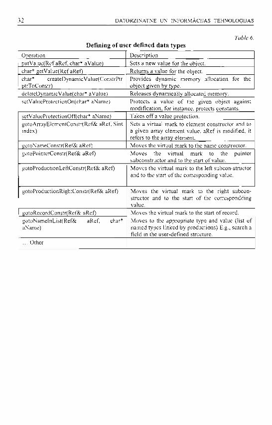
Table 6. Defining of user defined data types

Operation Description putValue(Ref aRef, char* aValue) Sets a new value for the object. char* getValue(Ref aReO Returns a value for the object. char* createDynamicVaIue(ConstrPtr ptrToConstr)

Provides dynamic memory allocation for the object given by type.

deleteDynamicValue(char* a Value) Releases dynamically allocated memory. setValucProtectionOn(char* aName) Protects a value of the given object against

modification, for instance, protects constants. setValueProtectionOff(char* aName) Takes off a value protection. gotoArrayElementConstr(Ref& aRef, Sint index)

Sets a virtual mark to element constructor and to a given array element value. aRef is modified, it refers to the array element.

gotoNameConstr(Ref& aRef) Moves the virtual mark to the name constructor. gotoPointerConstr(Ref& aRef) Moves the virtual mark to the pointer

subconstructor and to the start of value. gotoProductionLeftConstr(Ref& aRef) Moves the virtual mark to the left subcon-structor

and to the start of the corresponding value.

gotoProductionRightConstr(Ref& aRef) Moves the virtual mark to the right subcon­structor and to the start of the correspondding value.

gotoRecordConstr(Ref& aRef) Moves the virtual mark to the start of record. gotoNameInList(Ref& aRef, char* aName)

Moves to the appropriate type and value (list of named types linked by productions) E.g., search a field in the user-defined structure.

... Other

Guntis Aniicuns. D e s c r i p t i o n of S e m a n t i c s a n d C o d e G e n e r a t i o n Poss ib i l i t i e s 33

Table 7. Operations with variables and similar objects

Operation Description ConstrPtr create Constr Array (Uint min Index, Uint maxlndcx, ConstrPtr ptrTo ElemConstr)

Defines an array type with the given dimensions and element types. Here and in other functions we can use any previously defined (or partly defined) data type.

ConstrPtr createConstrFunct (ConstrPtr ptr To Return Constr, ConstrPtr ptr To Param Constr)

Defines a function type with the given parameters and return type.

ConstrPtr createConstrName(char* aXame, ConstrPtr trToSubConstr)

Assigns a user-defined name for the given type.

ConstrPtr createConstrPointer(ConstrPtr ptrToSubConstr)

Defines a pointer type to the given type.

ConstrPtr ereateConstrProduct(ConstrPtr ptrToSubConstr], ConstrPtr ptrToSubConstr2)

Creates a production of two types (establishes some relation between them). It is useful to construct a serious data structure.

ConstrPtr createConstrRecord(ConstrPtr ptrToSubConstr)

Defines a record data type (a set of pairs [name, tvpe}).

... Other constructors For instance, base data type constructors constr ArraySetMinIndex(ConstrPtr ptrToConstr, Uint minlndex)

Modifies the type description (attributes).

Uint constrArrayGetMinIndex(ConstrPtr ptrToConstr)

Provides details about data type attributes.

... Others

Table X. Operations with value

Operation Description Create Var (char* aName, ConstrPtr ptrToConstr)

Creates a variable with the given name and type.

createVar(char* aName, char* typeName) Creates a variable with the given name and type name.

createLiteral (char* aName, Constr Ptr ptrTo Constr)

Creates a literal (constant) with the given name and type.

Ref createRef (ConstrPtr ptrToConstr) Creates an object without a name with the given type, for instance, internal loop counter, return value of function.

[ ConstrPtr getConstrRef (char* typeName) Returns pointer to type with the given type name.

createSynonym (char* aName, Ref aRef) Creates another reference by name to the existing object.

... Other

L A T V I J A S U N I V E R S I T A T E S R A K S T I . 2 0 0 4 . 6 6 9 , sfej.: D A T O R Z I N A T N E L'N I N F O R M A C I J A S T E H N O L O G I J A S . 3 4 . - 5 2 . Ipp.

Data Staging in the Data Warehouse Janis Benefelds

Compute r Science Ph.D. s tudent . Univers i ty of Latvia J a m s . Be note klst» u n i b t m k a . l v

This topic describes one of Data Warehousing components - Data Staging. Data staging ensures a) data extraction from the source systems: b) data transformation and standardisation; c) data transfer to the Data Warehouse. The Importance of such important things like data quality and data integrity is described in more details too. This paper intends to be a survey based on practical experience in real projects and theoretical professional literature studies. The Paper consists of a Foreword, six Chapters and References. The Foreword describes the scope or the subject to be analysed in this article. The first Chapter is an introduction that gives definitions and common understanding about concepts used in this article The second Chapter is the largest one. and it describes three main parts of Data transformation Staging: data export, data transform and data load. Two types of Data Staging - dimensional and fact table staging - are described in more details. This Chapter is concerned with relative problems, like data quality, as well. The third and fourth Chapters describe such an important component of Data Staging like Metadata and the mutual relation between it and other parts of Data Staging described in the previous Chapter. The Fifth Chapter summarises the more important items and makes emphases on them to understand how essential they are to be successful in Data Staging. The Sixth Chapter points out the directions that follow as logic and sequential continuation to be a subject for further research and analysis References contains a list of information sources. Key words: metadata, data warehouse, data staging, data integrity.

Foreword

This article is a summary about Data S tag ing as one of the components of Data Warehous ing . There is an explanat ion of Da ta Staging — w h a t it means and what it consists of. Some c o m m o n definitions are given and the basic e lements (data extraction, t ransformation, loading and metadata) arc descr ibed. The content is additionally illustrated by many examples that are taken from the financial industry.

This Art icle points out the importance of the right unders tanding of the functions which Data Staging is responsible for, to be successful in designing and deploying projects in real life.

The following picture (Figure I) shows the basic Da ta Warehous ing e lements and describes what part of it this article covers .

Janis ttene Data Stat­ in the Da ta W a r e h o 35

Data Sources

Data Staging Area

Data Export

Data Transform j

I — i

Data Load

Data Warehouse

End User Applications

Metadata

Figure I' The basic elements of Data Warehousing

1. Introduction

Data Staging is one of the first and one of the mos t important things, if we arc discussing issues about deve lop ing a Data Warehouse.

In a lot of books , the Internet and other sources we can find numerous Data Staging definitions that are very similar. I would like to mention s o m e of them that would be sufficient and describe all the main functions performed by Data Staging.

Data Staging is a set of processes that cleans, transforms, combines, deduplicates. households, archives and prepares source data for use in the Data Warehouse.

Data Staging Area is everything in between the source system and the presentation server where Data Staging processes are performed. The key defining restriction on the Data Staging area is that it does not provide query and presentation services to end-users.

The Data Staging area is the Data Warehouse workbench. It is the place where raw data is loaded, cleaned, combined, archived and exported to one or more presentation server platforms.

One of the D W H gurus , Ralph Kimbal l , has ment ioned that Data Staging adds to the data an additional va lue , e.g.. the data quality and sense of use of these data in some analysis is higher than before. In general the Data S tag ing process consists of one c o m m o n service componen t - metadata - and three functional components :

• Data Export from the source systems or data consol idat ion;

• Data cleaning, t ransforming and soil ing or data s tandardizat ion;

• Data import into the Data Warehouse . Data Mart or loading:

36 D A T O R Z I N A T N E U N I N F O R M A C I J A S T E H N O L O G I J A S

There may be some different abbrev ia t ions used to n a m e these processes . E T L stands for Export . Transfer and Load, E T T s tands for Extract ion, Transformat ions and Transporta t ion. In this article we ' l l use ETL.

It certainly does not mean that Da ta S tag ing consists of three strictly different modules , where the sequence and comple t enes s of tasks to be performed is highly prescribed. Data Staging, depending on the si tuat ion, can be very a compl ica ted process from the functional and technical point of v iew.

It is r ecommended to start the Data S tag ing design process with a very simple schemat ic of the pieces that you know: the sources and targets. Keep it very high-level and highl ight where data are coming from and where data are going to , point out the major chal lenges that you already k n o w about . Figure 2 shows an example of a high-level Data Staging design plan that c a m e from the financial industry.

Figure 2: Example of the high-level Data Staging plan for some financial institution.

For a better unders tanding of the pr inciples and mission of Data Staging, le t ' s analyse each of the three steps ment ioned before m o r e closely.

2. ETL

2.1. Data export from transactional systems or data consolidation.

Practically every on-l ine t ransact ional system (OLTP) used in organizat ion is a potential data source for the Data Warehouse . H o w e v e r a data source for the Data Warehouse can be some external informat ion sys tems and not classified information

Janis Benefelds. D a t a S t a g i n g in the D a t a W a r e h o u s e 37

(flat files etc.) as wel l . Everything that serves as a data source can be developed in different envi ronments on different platforms and it can be " h o m e - m a d e " and delivered by external vendors . From the point of view of the Data Warehous ing it should make no difference - the only thing w e are interested in is data.

Normal ly , the scope o f the data to be collected in the Data Warehouse is defined by the end users - usually business people . Tha t means the scope is defined in business not Information Technology concepts and therefore high quali ty business analysts and system analysts are required at this stage of the Data Warehous ing process.

To determine the right database objects (and their relat ionship) that potentially could be included in a data export processes , business analysts should very precisely define the requirements of data needed and the system analyst should be able to point out how and where these data physical ly can be allocated. Normal ly the system analyst uses the system documenta t ion that should help to find out the right information about data wi th in a system. Sadly , there m a y be situations when documenta t ion does not help, or there is no documenta t ion at all. Such a situation can arise because of poor managemen t during sys tem development , implementa t ion and maintenance processes. Then the only source of information about the inside of a part icular information system are people . Some kind of interviews should be organized and system documenta t ion , should be redesigned accordingly to the actual status of the system.

One of the result ing documents of these interviews is a data dict ionary and it is actually a part of the metadata (see chapter 3 .Metadata) . A Data dict ionary is a collection of descript ions of the data objects or i tems and their relationships in a data model . A data dict ionary can be consulted to unders tand where a data i tem fits in the structure, what values it m a y contain and basically wha t the data item means in real-wor ld t e rms . A small example of that part, which explains what the data i tem means in r ea l -wor ld terms, is shown in the fol lowing table.

Table No. I "Example of a Data dictionary from the financial industry"

Real-world term Database object and its relationship Account (Acct) One record of the table ACCOUNTS Active Acct Dormant Acct

Closed Acct

Accounts.Status = 1 AND Accounts.CloseDate IS NULL Accounts.Status = 2 AND <&today> - Accounts.LastTranDate > 3M Accounts.Status = 2 AND Accounts.CloseDate <= <today>

Client One record of the table CLIENTS Active client Dormant client Closed client

Client that has at least one active account (see 'Active Acct') Client with all accounts being dormant (see 'Dormant Acct') Client with all accounts being closed (see 'Closed Acct')

Using such a data dict ionary improves the efficiency of communica t ions between business and IT people . There should be no quest ions about what the business people are requir ing and where it can be found.

W h e n we have clarified what data is needed and where it can bee al located, we should give an answer to the question " h o w " the data can be extracted or exported from the part icular data source. Usually the first step[s] of the technical solution is very close

D A T O R Z I N A T N E U N I N F O R M A C I J A S T E H N O L O G I J A S

to the technical solution of the data source itself. It means a special program should be developed that extracts specific data from all data sources and puts it together in a Data Staging area. Figure 3 shows a small s chema of data extract ing from the different data sources and gathering the particular data together in the Data Staging area. Some financial figures of the cus tomers are taken to build a cus tomer profile.

At the Start of building the Data Staging applicat ion the pr imary goal is to work out the infrastructure issues, including connectivi ty, securi ty and file t ransformation.

Figure 3: An Example of data extraction processes from different data sources and putting it together in the Data Staging area.

Certainly data in a Data Staging area are stored in some particular structure and therefore the way in which the data c o m e s into these structures should be strictly predefined and complete ly documented . The n a m e of such a document is data mapping. Data mapping shows a complete way in which the par t icular data from some source system is transported (and transformed in be tween if necessary) to a Data Staging area.

Corresponding to a dimensional data model (general ly that is a data model for the Data Warehouse) there are two different types of Data Staging, each for one of two main components of the dimensional mode l : d imens iona l Data Staging and fact Data Stasiimi.

Dimensional Model - a specific discipline for modelling data that is an alternative to entity-relationship (ER1 modelling.

Janis Benefelds. D a t a S t a g i n g in the Data W a r e h o u s e 39

A fact tabic is the primary table in each dimensional model that is meant to contain measurements of the business. The most useful facts arc numeric and additive. Every fact table represents a many-to-many relationship and every fact table contains a set of two or more foreign keys that join to their respective dimensional tables.

A dimensional table is one of a set of companion tables to a fact table. Each dimension is defined by its primary key that serves as the basis for referential integrity with any given fact table to which it is joined. |

2.1.1. Dimensional tabic staging.

There are three types of processing dimensional data: overwrite , create a new dimension record, and displace the changed value into an "o ld" attribute field. The second one is the technique usually used for handl ing occasional changes in a dimension record. W e shall actually focus on that type of dimensional data processing.

In terms of complexi ty the major problem could be the identification and extraction of data that has been changed since the last data extraction instead of extraction of all data every t ime. It is convenient to have a mechanism to select new or changed data only. Ideally there is an additional column in the source data that shows the last change date and t ime or jus t a yes /no s tamp that indicates whether the particular data is or is not changed since the last data extraction. That means that only these data will be the subject of the Data Staging. Taking into account that usual ly some of the data source information systems are either delivered by an external vendor or long ago " in -house" systems without any knowledge about their contens and without full documentat ion, there may be some p rob l ems to change these systems for having such a s tamp indicating a change status according to the last data extraction process . That means there should be another way to de te rmine the existence of the new records and changes in the old ones. In this case the easiest way is to pull the current snapshot of the dimension table in its entirety and let the t ransformation process deal with de te rmining what has changed and how to handle it. C h a n g e determinat ion could be done by compar ing the actual data snapshot either with yes te rday ' s data snapshot or with the current Data Warehouse dimensional table. This way is more t ime-consuming and complicated, f igure 4 shows data flow for this type of d imensional Data Staging.

Data source Today's

dimensional table data

Data source Today's

dimensional table data

Yesterday's dimensional

table data

/ Compare -»•-. and allocate

Vdifl'crences/

New Records to be inserted in the D W I I

dimension table

Surrogate key

. G e n e r a t i o n ,

Figure 4: Allocation of new and changed records in dimension data

40 D A T O R Z I N A T N E U N I N F O R M A C I J A S T E H N O L O G I J A S

Because of the large amount of data to be extracted, compared (or transferred), special attention to usage of software and ha rdware resources should be paid. Special comparison methods could be used for per formance improvement , such as the Cyclic Redundacy Checksum ( C R C ) . This me thod calculates a checksum for a particular string - it could be a record of a table or a whole text file or something else. The checksum calculated for the new data is then compared with the checksum of the yes te rday ' s data that is already calculated. If these checksums are equal there is no need to compare details for part icular details. The Usage of such methods substantial ly saves lime and hardware resources.

2.1.2. Fact table staging

Facts usually represent a snapshot of a data source at that part icular t ime point. Accordingly facts normal ly are the numer ic at tr ibutes of the subject of the transactional system, like daily balance of an account , sales amoun t of a product , etc. Problems regarding extracting of such data from the data source normal ly are connected with the amount of data to be processed and wi th the changeabi l i ty of data. Problems regarding data amounts usually can be solved on account of technical issues or data processing performance optimization. A lmos t every t ransact ional sys tem provides today on-line services and that means t ransact ions are per formed all the t ime (24hours /7days) . The problem grows even b igger in case of a mult inat ional sys tem, where many t ime zones are involved. To get a snapshot of such a sys tem in the part icular t ime point , some technical tricks can help. There can be several solut ions. In current data base management systems, l ike Oracle, a backup technology is provided without disconnect ing users or shut t ing d o w n a data base - a back-up is created taking into account the events in the system logs. Accord ing ly fact data could be extracted from a back-up or directly from the system using the same technology. Actual ly , normally every system has some housekeep ing phase for suppor t ing some internal functionality (like E O D - end of day) that makes a sys tem constant for some t ime. Whe the r the sys tem serves business t ransact ions or not dur ing this t ime-out depends on the particular system - there are some dist inct ions. Such t ime-out is a good place for fact data (and dimensional data as well) extract ing.

Conclusion.

The Financial industry differs from the other major sectors of bus iness with its non­stop business . Because of many channels ( A T M , Internet , W A P . etc.), which banks provide, the customer has the possibil i ty to do business all the t ime any day. A Similar situation exists in the te lecommunica t ion business as well.

That is the N°l problem for data extract ion, which should be solved. Normal ly every IS operat ing in the financial industry has already solved the problem of on-line t ransact ions. There are s o m e techniques that ensure on-l ine data process ing and daily (weekly, monthly , etc.) data servicing at the same t ime. These data servicing procedures (housekeeping , calculat ions, etc.) could be popula ted with data extraction.

Problem N°2 is the large amount of he te rogeneous data (funds transfers, loan agreements , securities, trust operat ions , insurance, etc.) to be processed. That could be solved by 1) using opt imal data a l locat ing a lgor i thms to find data to be processed and 2) fast data extraction mechan i sms . A Data al locat ing mechan i sm could be, for instance.

Janis Benefelds. D a t a S t a g i n g in the Da ta W a r e h o u s e 41

Cyclic Redundacy C h e c k s u m method or using different ' changed da ta ' flags in the source sys tems. As fast a data extraction mechanism specific tools could be used or just making a copy and process ing 9 0 % of data instead of selecting 9 0 % of data and processing all of the resul t ing data set.

2.2. Data cleaning, transforming and sorting or data standardization

This is the place where an addit ional value to the data actually is added.

Usually there are some activities be tween data extract ion from data source systems and data import into the data target. These activities ensure that data in the right structure, format, and sequence , and that quality should be adequate for the data model of the data target. The Data should satisfy all logical rules provided by business analysts and all physical rules that come from the Data Warehouse data model and end user applications.

2.2.1. Data quality

Actually, most of all data transformation deals with data quality.

There is no reason to assume the quality of data in O L T P systems a lways will be acceptable for the Data Warehouse . S o m e data validations can be integrated directly in the source (OLTP) to preserve data from logical and structural mistakes. In any case, there are some prob lems . First - every data validation procedure makes the system slower and it conflicts with a definition of the O L T P "on-l ine (identical "fast") t ransaction process ing" . Second - even if we create all necessary data validations in O L T P , there always will arise some new requirements or condit ions against data to be realized in the Data Warehouse . It is easier, cheaper and more secure to realize data cleaning and t ransformation procedures outside of the data source.

In the Situation when data are val idated after they have been captured, another problem arises - how to edit them n o w ? If a validation error occurs by data capture, they can be entered once more till they are correct. Whereas if a data validation error is discovered during a fully automated data cleaning and standardizat ion process , there should be some previous ly described algori thms to m a n a g e the situation. Automatic data edit ing algori thms should be approved by business analysts and every data change should be stored in the L O G files.

Wherever and wheneve r data are modified before import ing them into the Data Warehouse , they should be at the best quality possible. There are attributes that indicate the level of data quality.

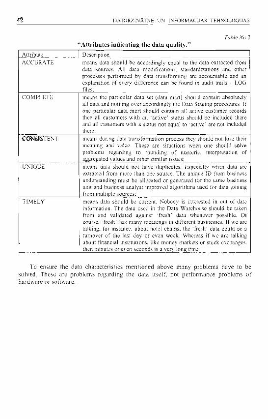
42 D A T O R Z I N A T N E U N I N F O R M A C I J A S T E H N O L O G I J A S

Table No.2 "Attributes indicat ing the data qual i ty ."

Attribute Description ACCURATE means data should be accordingly equal to the data extracted from

data sources. All data modifications, standardizations and other processes performed by data transforming arc accountable and an explanation of every difference can be found in audit trails - LOG files;

COMPLETE means the particular data set (data mart) should contain absolutely all data and nothing over accordingly the Data Staging procedures. If one particular data mart should contain all active customer records then all customers with an 'active' status should be included there and all customers with a status not equal to 'active' are not included there;

CONSISTENT means during data transformation process they should not lose their meaning and value. These arc situations when one should solve problems regarding to rounding of numeric, interpretation of aggregated values and other similar issues;

UNIQUE means data should not have duplicates. Especially when data are extracted from more than one source. The unique ID from business understanding must be allocated or generated for the same business unit and business analyst improved algorithms used for data joining from multiple sources;

TIMELY means data should be current. Nobody is interested in out of date information. The data used in the Data Warehouse should be taken from and validated against 'fresh' data whenever possible. Of course, 'fresh' has many meanings in different businesses. If we are talking, for instance, about hotel chains, the 'fresh' data could be a turnover of the last day or even week. Whereas if we are talking about financial institutions, like money markets or stock exchanges, then minutes or even seconds is a very long time.

To ensure the data characterist ics men t ioned above many problems have to be solved. These are p rob lems regarding the data itself, not performance prob lems of hardware or software.

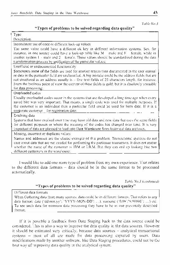
Janis Benefelds. D a t a S t a g i n g in the Data W a r e h o u s e

Table ho. 3 "Types of problems to be solved regarding data quality"

Type Description Inconsistent use of code or different look-up values The same value could have a different ok key in different information systems. Sex, for instance, in one source could have a look-up table like M - male and F - female, while in another system I - male and 2 female. These values should be standardized during the data transformation process by unification of the particular values; Unofficial or undocumented functionality Sometimes some of the fields are used for another reason than documented in the user manual or data in the particular field are unclassified. A big mistake could be the address fields that arc not structured as an address usually is - five text fields of 25 characters length, for instance. From the business point of view the content of these fields is gold, but it is absolutely unusable for data processing; Overloaded codes Usually overloaded codes occur in the systems that are developed a long time ago when every saved bite was very important. That means, a single code was used for multiple purposes. If the customer is an individual then a particular field could be used for birth date. If it is a corporate customer - for registration date: Evolving data Systems that have evolved over time may have old data and new data that uses the same fields for different purposes or where the meaning of the codes has changed over time. It is very important if data are planned to load into Data Warehouse from historical data archives; Missing, incorrect or duplicate values Names and addresses are the classic example of this problem. Transactional systems do not care about data that are not needed for performing the particular transaction. It does not matter whether the name of the customer is IBM or I.B.M. But they can end up looking like two different customers in the warehouse;

1 wou ld like to add one more type of problem from my o w n experience. That relates to the different data formats - data should be in the s ame format to be processed automat ical ly .

Table No. 3 (continued) "Types of problems to be solved regarding data quality"

Different data formats When Gathering data from many sources, data could be in different formats. That refers to any . data format: date Cdd.mm.yy'; 'YYYY-MON-DD': . . . ) . numeric C0.99':'9.9999E"; ...) etc. To use such data for common data processing they have to be in one previously described format;

If it is poss ible a feedback from Data Staging back to the data source could be considered. This is also a way to improve the data quality in the data sources. However it should be es t imated very critically, because data sources - analytical t ransactional systems — most of all are made for data process ing captured by users. Data modif icat ions made by another software, like Data Staging procedures , could not be the best way of improving data quality in the analytical system.

44 D A T O R Z I N A T N E UN I N F O R M A C I J A S T E H N O L O G I J A S

2.2.2. Data integrity

Besides data quality this part of Data Staging is responsible for data integration as well. Ensur ing of data integrity means surrogate key (as pr imary key) generat ion for dimensional data tables and fact table popula t ion (or even creat ion) using jus t generated surrogate keys. All d imens iona l tables have single part keys , which, by definition, are primary keys. In other words , the key itself defines un iqueness in the dimensional tables. It is a significant mis take to use, for uniqueness of d imensional table record, an SQL-based date s tamp, a set of various at tr ibutes in the d imens iona l table, production keys used in the data source . In most cases an integer m a k e s a great surrogate key. A 4-byte integer, for instance, can contain 2 ? ~ values , or m o r e than two billion positive integers starting with 1, and that is enough for jus t about any dimension.

Since fact tables are a lways associated with d imensional tables, surrogate keys should replace corresponding foreign keys there. Figure 5 shows a dimensional data model where generated surrogate keys (T ime_key , Cus tomer_key , A c c t k e y ) of dimensional tables are used as foreign keys in the fact table instead of product ion keys (Date. Ct is tomer_ID, A c c t _ l D ) .

Time dimension Customer dimension

Time_key (PK) Date Day_of_week Day_of_year Week_number etc.

Daily balance fact table

Account dimension

Acct_key (PK) Acct ID Acct type Currency Ledger_balance etc.

T i m e k e y (FK) Acct_key (FK) Customer_key (FK) Ledge rba l Acct_ccy Ledger_bal 1 Base ccy

Customer_key (PK) Cus tomer lD Customertype Name Address etc.

Figure 5: Example of using surrogate keys instead of production keys in the Daily balance fact table

For better query ing per formance besides dimensional and fact data, the Data Warehouse has the aggrega te date as wel l . Since the Data Warehouse is used most of all to get summarized data over any d imensional at tr ibutes, a significant data aggregation would be performed by every data request . Therefore data base management systems provide an opportuni ty to maintain aggregated data - mater ia l ized v iews or data where subtotals are already calculated up to a predefined level of granulari ty. Figure 6 shows how an aggregate data table is handled that ensures answer to data query about product sales subtotals for a part icular week or a few weeks .

Janis Benefelds. D a t a S t a g i n g in the Da ta W a r e h o u s e 45

Aggregate Daily Time dimension balance fact table

Day_of_year (FK) Acct_key (FK) SUM(Ledger_bal) MIN(Ledger_baI) iMAX(Ledger_bal) AVG(Ledger_bal) Acct ccy SUM(Ledger_bal 1) MlN(Ledger_baI 1) MAX(Ledger_ball) AVG(Ledger_ball) B a s e c c y

=>

Time_key (PK) Date Day of week Day of year Week number etc.

Product dimension

Sales fact table

balance fact table

Day_of_year (FK) Acct_key (FK) SUM(Ledger_bal) MIN(Ledger_baI) iMAX(Ledger_bal) AVG(Ledger_bal) Acct ccy SUM(Ledger_bal 1) MlN(Ledger_baI 1) MAX(Ledger_ball) AVG(Ledger_ball) B a s e c c y

=>

Time_key (PK) Date Day of week Day of year Week number etc.

Product dimension

• « T i m e k e y (FK) Acct key (FK) Customer key (FK) Ledger bal Acct ccy Ledger ball Base ccy

balance fact table

Day_of_year (FK) Acct_key (FK) SUM(Ledger_bal) MIN(Ledger_baI) iMAX(Ledger_bal) AVG(Ledger_bal) Acct ccy SUM(Ledger_bal 1) MlN(Ledger_baI 1) MAX(Ledger_ball) AVG(Ledger_ball) B a s e c c y

Acct_key (PK) A c c t J D Acct_ type Currency Ledger balance etc.

• « T i m e k e y (FK) Acct key (FK) Customer key (FK) Ledger bal Acct ccy Ledger ball Base ccy

Figure 6: Example of the aggregate Daily balance fact table.

Conclusion.

I would say that data quality is one of the major uni ts of measure (the second one is data accessing per formance , but that is not the subject of this topic) for the Data Warehousing. The benefi t that users obtain from the usage of the data warehouse is as large as how clean and good are the data. So, if data are inaccurate, the user gets the wrong picture of the bus iness and a decision that is based on that picture could be wrong.

N o recourses should be economized to improve data quality. Regarding the data that banks capture and mainta in themselves - that is all their own business, and they do everything to avoid ' d i r ty ' data. Somet imes a solution could be some administrat ive order to stop doing things in the wrong way. Data that w e get from outside of the bank, or even the financial industry, should have a warranty, e.g., the data supplier should be trustworthy and secure enough . Usually these are some state institutions, but they could be some commercia l organisat ions ( insurance companies , travel agencies, etc.) as well -contract about providing data should contain requirements and warranties regarding data quality and security.

A separate Data Qual i ty depar tment within the organisat ional structure would help significantly as well. Such a depar tment could deal with 'd i r ty ' data - to ensure the certain level of the data quality by developing data transformation and cleaning algori thms as well as looking for some external data sources that could serve as a standard for data compar ison .

2.3. Data loading into the Data Warehouse, Data Mart or data loading

Data loading into the Data Warehouse means physical data transportat ion from the Data Staging area (da tabase A) to the Data Warehouse (database B). To populate an existing database with new data usually some data managemen t p rob lems should be

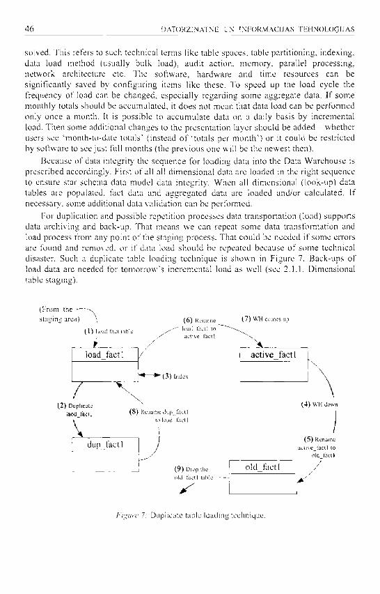
46 D A T O R Z I N A T N E U N IN F O R M A C ! J A S T E H N O L O G I J A S

solved. This refers to such technical terms like table spaces, table part i t ioning, indexing, data load method (usually bulk load), audi t action, m e m o r y , parallel processing, network architecture etc. The sof tware, hardware and t ime resources can be significantly saved by configuring i tems like these. To speed up the load cycle the frequency of load can be changed, especial ly regarding some aggregate data. If some monthly totals should be accumula ted , it does not mean that data load can be performed only once a month. It is possible to accumula te data on a daily basis by incremental load. Then some additional changes to the presentat ion layer should be added - whether users see 'month- to-date to ta ls ' ( instead o f "totals per m o n t h ' ) or it could be restricted by software to see just full months (the prev ious one will be the newest then).

Because of data integrity the sequence for loading data into the Data Warehouse is prescribed accordingly. First of all all d imens iona l data arc loaded in the right sequence to ensure star schema data model data integrity. When all d imensional ( look-up) data tables are populated, fact data and aggregated data are loaded and/or calculated. If necessary, some additional data validation can be performed.

For duplication and possible repetition processes data t ransportat ion ( load) supports data archiving and back-up. That means we can repeat some data transformation and load process from any point of the staging process . That could be needed if some errors are found and removed, or if data load should be repeated because of some technical disaster. Such a duplicate table loading t echn ique is shown in Figure 7. Back-ups of load data are needed for t o m o r r o w ' s incremental load as well (see 2 .1 .1 . Dimensional table staging).

( F r o m the —-

s t a g i n g a r e a )

(1) Load tact table ( 6 ) Rename liiad tact 1 to active tact I

load factl

•(3) Index

/ 3up!ie; L-CK! _ f a<

i (2) Duplicate

b o d j a c l I ( 8 ) «<"P.foa' to load tact 1

dup fact 1

(9) Drop l!ie okl tact I table

(7) W H comes up

act ive factl

old factl

(4) W H down

(5) Rename acme factl to

old tact I

Figure 7: Duplicate table loading technique.

Janis Benefelds. D a t a S t a g i n g in the Data W a r e h o u s e 47

Step 0 The active_factl table is active and queried by users. Step 1 The load_fact I table starts off being identical to active_fact I.

Load the incremental (different) facts into the load_factl table. Step 2 Duplicate load fact 1 into dup_factl for tomorrows load. Step 3 Index Ioad_faet I table according to the final index list. Step 4 "Bring down" the warehouse, forbidding user access. Step 5 Rename the active_factl table to old_factl (back-up). Step 6 Rename the loadfact l to ac t ivefact l . Step 7 Open the warehouse to user activity. Total downtime: seconds! Step 8 Rename the dup_factl tabic to load_factl for performing of next load. Step 9 Drop the old_factl table.

3 . Metadata

S o m e tools that au tomate the transformation and load layer can actually reside on a third party platform and generate the code necessary to perform those activities (see Figure 8 as well). And the most important thing that ensures such a possibili ty is metadata.

The definition of metadata is really s imple - metadata is data about data. Does it help a n y b o d y to unders tand what exactly this elusive information? In my opinion - no. More descr ipt ive definition could be as follows. Metadata is all of the information (or descript ive information) in the particular envi ronment that is not the actual data itself. Some authors are even talking about the "back room metadata" and "front room metadata" . The back room metadata is process related and it guides the data extraction, cleaning and loading process . The front room metadata is more descriptive and it helps query tools report wri ters function smooth ly . Of course , both metadata types overlap, but it is useful to think about them separately. In this case we are interested in the first one - back room metadata.

Metada ta is like traditional systems documenta t ion (in fact, it is documenta t ion) and at s o m e point the resources needed to create and maintain it will be diver ted to other "more u rgen t" projects. Act ive metadata helps solve this problem. Act ive metadata is metadata that drives a process rather than documents it, while documenta t ion of these processes is an important issue as well.

The following is the general metadata needed to get the data into the Data Staging area and prepare it for loading into one or more data marts .

Data extraction information

• Descr ip t ion of the source systems (schemas , formats etc.);

• Access methods , r ights, privileges and passwords ;

• Da ta t ransportat ion scheduling and results of them:

• File usage in the Data Staging area including durat ion and ownership:

Data t ransformation information

• Data model :

• Job specifications for joining sources , s tr ipping out fields and looking up at tr ibutes:

48 D A T O R Z I N A T N E UN I N F O R M A C U A S T E H N O U O C I J A S

• Data mapping be tween sources and Data Staging area;

• Yesterdays copy o f production data to use as the bas is for DIFF C O M P A R E

• Data update (refreshing) policies for each incoming at tr ibute;

• Current surrogate key ass ignments and me thodo logy of that;

• Data cleaning, formatt ing, filtering and sort ing:

• Populat ing data for data mining (e.g. , interpret nul ls , scale numerics etc.);

Data load information

• Target schema des ign, source-to-target (s taging area to data mart) data flows and target data ownership;

• D B M S load scripts;

• Aggregate definitions;

• Data (especial aggrega te ) usage statistics and potent ial improvements ;

Audit , Job Logs and Documenta t ion

• Audit records (where exact ly did this record come from and when?) ;

• Data transform run t ime logs, success summar ies and time stamps;

• Information about software (version numbers ) and ha rdware (configuration);

• Security sett ings;

Conclusion.

Metadata is an important issue in terms of descr ipt ions . It describes (it should at least) any object and any process deal ing with these objects . It is very hard to define or to show - this is metadata and that is not . The content o f metadata usually describes the structure or nature of o ther data (the real ones) . Metada ta , for instance is ER diagram, description of table s t ructures , documenta t ion of the p r o g r a m packages etc.

4. Relationships between Export, Transfer and Load.

A s I have already ment ioned data extract ion, t ransformat ion and load are very closely related to each other on the one hand (usually in the small projects) and these parts could be very strictly separated on the other hand (large projects somet imes use separate software products to manage data ext ract ion, t ransformation, loading and metadata in their ent irety) . Somet imes it is really impossible to strictly separate which piece of software or ha rdware belongs to one part of Data Staging and which one to another. For instance, let us say we have jus t one data source system, which operates in the Oracle, and data should be loaded in the Data Warehouse , which is developed in an Oracle environment too . If hardware and software configurat ion al lows creating a database link between these t w o Oracle databases , then Data Staging could be jus t one SQL statement. Of course , it is a very simplif ied example , but it is true:

Janis Benefelds. D a t a S t a g i n g in the Data W a r e h o u s e 49

INSERT INTO CUSTUM_DIMENSION ( SELECT NEXTVAL.cust_seq cust_pk, cust_id, cust_name, TOJ3ATE(birth_date. 'DD.MM.RRRR - )birth_date. DECODE(scx,' 1 7 M 7 F ' ) sex FROM CUSTOMERS@;SOURCE ORDER BY cusMd )

And there we can see:

Data extraction:

Data transformation:

Data transportation:

SELECT cust_id, cus tname. birth_date. sex F R O M C U S T O M E R S ® S O U R C E NEXTVAL . c u s t s e q - surrogate key generation TojDATE (bir thdate . 'DD.MM.RRRR') - data fomiat adjustment D E C O D E ( s e x , ' L / M \ ' F ' ) - unification of code keys ORDER BY cust_id - particular record order INSERT INTO CUSTUM DIMENSION

It actually means that from the technical point of view Data Staging looks like Figure 8.

Da ta sources

Extract and | transformation

programms J

Data m o v e m e n t

Data m o v e m e n t

• > Cleans ing ,

t ransformat ion . sor t ing p r o g r a m m s l

Data W a r e h o u s e

Transformation, addition, update

programms I

Figure S: Role of data transformation and transportation tools within a Data Staging process.

50 D A T O R Z I N A T N E L'N I N F O R M A C I J A S T E H N O L O G I J A S

5. Summary

As a conclusion 1 would say that Data Staging is one of the main issues of the Data Warehousing one must pay much at tention to. Data Staging covers any action with data starting from extracting them from the source systems and finishing with data loading into the presentation server (Data Warehouse and 'o r Data Mart ) . Data Staging itself does not include data presentat ion, e.g., data cannot be accessed by the end users from the Data Staging area. Data Access by end users is performed by other tools. Actions that Data Staging performs arc (at least, should be) very short in t ime, whereas the developing of these processes could take much of t ime and many other resources.

The main tasks of Data Staging are 1) fast part icular data extraction from the source systems 2) fast data t ransformation, s tandardizat ion and data quality assurance according to the business user requi rements and 3) fast data loading into the target according to the data model (usually d imens iona l ) it requires .

Nowadays technologies usually prov ide a range of possibil i t ies to ensure fast physical data processing and t ranspor ta t ion - I wou ld say. that should solve all problems regarding physical data extract ion, mov ing them through the hardware infrastructure and loading them into the data target, wha tever that may be. Besides that, the logical side of data process ing still should be taken into account. This part of the data processing brings out the impor tance of the human sense or intelligence that should be both the driver and supervisor of the manne r in which data is managed . That means Data Staging development requires addi t ional special skills and exper ience in the data management area. In the case of Data Warehous ing these special skills would be dimensional data model l ing and usage of and managemen t of the metadata . It could be reasonable to look toward some vendors that provide tools for the functionality jus t ment ioned (dimensional data model l ing and metadata managemen t ) . In any case, it is very good to have at least a theoretical background and unders tanding about how it should work. On the one hand there is no ready solution (software) that will satisfy you for 100% of your needs , and on the other hand you will never develop that functionality by yourself according to the budget , t ime and end user requi rement restrict ions. The truth is a lways in the middle!

The main deliverables (in terms o f the metada ta) of the Data Staging would be:

• Data dictionary

• Data mapping

o Data source to Data Staging area

o Data Staging area to data target

• Description of the data t ransporta t ion (extract, back-up and load)

• Data quality'' checklist

• Data transformation a lgor i thms and audi t trails

Conclusion Regarding the financial industry, data extract ion and consol idat ion is very

important in terms of comple teness and accura teness . Only comple te and accurate data give the right picture - c o m m o n trends and aggregates .

Janis Benefelds. Da ta S t a g i n g in the Da ta W a r e h o u s e 51

Aggregated information is usually passed to a c o m p a n y ' s managemen t , external supervisors and auditors. Each of them requires special and very similar information. They are different but comparable! Data requirements are both regular and on demand. This is a good way to show others that data is under control in o n e ' s company, especially if response t imes to irregular data requests are short enough.

Besides the c o m m o n trends financial institutions focus on particular individuals or companies as well. Therefore data of the particular individual can be evaluated in relation with common trends only part ly. T h e other, the larger part of an evaluat ion is based on a cl ient 's individual data — client profile. Actual ly , such approach to data analysis is part of Cus tomer Relat ionship Management ( C R M ) , which is very important for financial institutions. This is exact ly the reason why data quality should be the best possible. Banks , insurers and other financial industry players are market ing themselves as ones w h o are professionals in w h o m you can trust. And clients are expect ing an adequate att i tude: " S o , if you know everyth ing about my finances, why do you offer me a Gold Credi t card? My monthly income is by far insufficient to buy such a product!" Such a si tuation comes from unclean and in consistent data, and it leads to the customer that doubts whether the bank is deal ing with his many at a level that is professional enough.

6. Further research

Sequential ly the next part after Data Staging is Database - either Data Warehouse , Data Mart or by a special Data Mining tool predefined data structures.

Deve lop ing the right Data Model and overall data architecture strategy could be the direction of the next research. This includes understanding the difference between d imensional and traditional O L T P design practices.

Since Data Model is developed data is coming in. Data M a n a g e m e n t is a very important issue as well . By Data M a n a g e m e n t 1 mean such things like data storage solutions, fast data access problems and other problems similar to it. As data volumes accumula ted by Data Warehouse general ly are extremely large, a technical and architectural solution should be ready to process it. This part of the Data Warehous ing definitely is a subject for following research as well.

As Data Warehous ing products ( report ing, analysing, data mining etc. tools) are required by business, it is very close to the particular end users. Of course , every company has its own specific requi rements , but there are some c o m m o n specificities from industry to industry. Financial industry specificities and possible solut ions to them are good area for research and for having key knowledge too.

52 D A T O R Z I N A T N E U N I N F O R M A C I J A S T E H N O L O G I J A S

References

Kimball R., Reeves L., Ross M., Thornthwaite W. (1998), The Data Warehouse Lifecycle Toolkit, John Wiley & Sons, Inc.

Groth R. (1998), Data Mining, Prentice Hall PTR Inmon W. H., (1999). Building the Operational Data Store - Second Edition, John Wilev & Sons,

Inc. Oracle Corporation, (1996 - 2000), Oracle Documentation Library. Release 8.1.7 Kimball R., Merz R. (2000). The Data Webhouse Toolkit, John Wiley & Sons, Inc. Marco D. (2000). Building and Managing the Meta Data Repository. John Wiley & Sons. Inc. Todman C. (2001). Designing a Data Warehouse, Hewlett-Packard Company Greenberg P. (2001). CRM at the Speed of Light. McGrow-Hill Companies Imhoff C , Loftis L., Geiger J.G. (2001), Building the Customer-Centric Enterprise. John Wiley &

Sons, Inc. Kimball R., Ross M. (2002), The Data Warehouse Toolkit - Second Edition, John Wiley & Sons,

Inc.

L A T V I J A S U N I V E R S I T A T E S RAK.STI . 20IM. 6 6 9 . se j . : D A T O R Z I N A T N E U N I N F O R M A C U A S T E H N O L O G I J A S . 5 3 . - 6 0 . 1pp.

Generic Data Representation by Table in Metamodel Based Modelling Tool

Edgars Celms Institute of Mathemat ics and C o m p u t e r Science, Universi ty of Latvia

Raina bulv. 29 , LV-1459 , Riga, Latvia Edgars. Celms@,mii . lu.lv

The foundation of a metamodel based modelling tool is its flexible facility to declaratively define the modelling method, notation and tool support. One of the problems for such tools is generic data representation by table. The paper proposes a method for declarative definition of a table based on the logical metamodel. The most interesting aspect of this definition is the specification of element selection criterion. Some practical examples of table specification by the described method are also explained. Key words: modelling tool, generic table editor, metamodel, editor definition.

1. Introduction

Today there are a lot of model l ing tools on the market . Model l ing tools are designed to provide all that is necessary to support major areas of model l ing, including business p rocess model l ing , object-oriented and componen t modell ing with U M L [ 1 ] , relational data model l ing, and structured analysis and design, etc. Why is it not sufficient to use "ha rd -coded" model l ing tools? Let us consider, for example , the situation in business model l ing. On the one hand there exist several we l l -known business model l ing languages ( IDEF3[2] , ARIS[3] etc.), each with a set of tools support ing it. But there are also Activity d iagrams in U M L . whose main role now is to serve bus iness model l ing . There is G R A D E B M [4] - a specialized language for business model l ing and simulation. Thus for the area of business model l ing there is no one bes t or mos t used language or tool , and each of them emphasizes its own aspects. For example , G R A D E B M presents very convenient facilities for specifying performers of a task and its t r iggering condit ions. H o w e v e r any new language feature does not come for free, and the language becomes more compl ica ted for use. Therefore one universal bus iness model l ing language, which would support all wishes, would become extremely difficult for use in simple cases. U M L for this situation offers one ingenious solution — stereotypes for adjusting the model l ing language to a specific area. In many cases the idea works perfectly, and it is well supported in several tools including G R A D E . The latest version of U M L - 1.4 extends the notion of stereotype, by assigning tagged values to it and grouping stereotypes into profiles (thus actually ex tend ing the metamodel ) . But currently no tool fully supports it and already a new version of U M L -2.0 is coming with significant changes, part icularly in the area of Activity d iagrams.

The problem with flexible model l ing envi ronment is even more urgent for domain-specific model l ing , where countless special notat ions are used for separate domains .

There are probably several ways to solve such a problem.

You can develop a model l ing tool special ly for any specific modell ing method but this way can be very t ime and cost consuming.

54 D A T O R Z I N A T N E UN I N F O R M A C I J A S T E H N O L O G I J A S

You can make a tool as universal as poss ib le to support all needs. For example, there is ARIS tool by IDS prof. Scheer . whose "home notat ion" is the ARIS BM language. But it supports also the L'ML notat ion with Activi ty d iagrams, as well as numerous modifications of the main process notation via eEPC (office processes, industrial processes etc) . In general , A R I S tool can be character ised to be extremely "wide", with about 110 different types of d iagrams , and frequently having about 100 different symbol types per d iagram (most , in fact, are predefined stereotypes of the basic ones). At the s ame t ime, there are practical ly no facilities for defining new stereotypes. In practice such a universal tool is difficult for use in simple cases.

An alternative way is a complete ly metamode l based generic model l ing tool (previously called m e t a C A S E ) . Such a tool has no built-in model l ing methodology. It has to be filled up wi th specific metamode l and addit ional information to start modell ing something.

2. Metamodel Based Modelling Tool

In this paper some aspects of the m e t a m o d e l based approach to bui lding flexible modell ing envi ronments are explained. The metamode l concept has become popular in recent years especially due to the pr inciple used in L 'ML definition [1] . What is a metamodel in a metamode l based model l ing tool? To put it in short, a metamodel is a class diagram conta ining all model l ing concep ts , their at tr ibutes and their relationships. A metamodel based tool has no built-in mode l l ing methodo logy . It has to be filled up with specific metamodel and addit ional information to start model l ing something.

An earlier al ternative name for the approach is m e t a C A S E . Let me ment ion the key research in this area. Perhaps , the first s imilar approach has been made by Metaedi t [5], but for a long time its editor definition facilities have been fairly limited. The latest version named M e t a e d i t - now can support definition o f most used diagram types, but via very restricted metamode l l ing features (non-graphica l ) , the result ing diagrams corresponding to the simplest concept of labelled directed graph. The most flexible definition facilities (and some t ime ago , a lso the most popular in practice, but now the tool is out of the market) seem to be offered by the Toolbu i lde r by Lincoln Software. Being a typical m e t a C A S E of the early ninet ies , the approach is based on E R model for describing the repository contents and on special extens ions to E R notation for defining derived data objects wh ich are in a one- to-one relation to objects in a graphical diagram. A more academic approach is that p roposed by Kogge [6] , with a very flexible, but very complicated and mainly procedural edi tor definit ion l anguage . Other newer similar approaches are proposed by ISIS G M E [7], D O M E [8] and Moses [9] projects , with main emphasis for creat ing env i ronments for domain-speci f ic model l ing in the engineering world. The richest editor definit ion possibi l i t ies of them are in GME. Several commercial model l ing tools (ARIS by IDS prof. Scheer , System Architect by Popkin Software[10], etc.) use a similar approach internally, for easy customisat ion of their products, but their tool definition l anguages have never been made explicit.

The approach explained in this paper is in a sense a further development of the above mentioned approaches . In this approach at first the domain metamodel of the modelling area (logical metamodel ) is built . Then the mode l l ing method, notation and tool support are defined declarat ively , by means of a special metamodel l ing

Eitg&ri Celms. G e n e r i c D a t a R e p r e s e n t a t i o n by Table in M e t a m o d e l B a s e d M o d e l l i n g Tool 55

environment . These activit ies also require extension of the metamodel (adding some presentat ion classes) , but it is not relevant to the purposes of this paper.

A very significant part of the tool support in metamode l based model l ing tools is flexible data representat ion facilities. There are some main principles how data can be represented in model l ing tools:

• D iagrammat ic ,

• Hierarchical (e.g. "tree v iews") ,

• Data dict ionaries,

• Tables ,

• Object editors.

Obvious ly the mos t popular data representat ion form (model l ing notation) in any domain now is d iagram based. Therefore a very important part of the metamodel based approach is the Edi tor Definition Language (EdDL) for a s imple and convenient definition of a wide spect rum of d iagrammat ic graphical editors [11 . 12]. Never theless not all information is convenient to represent by d iagrams. There is also the necessity to have a possibili ty in metamode l based model l ing tools to define such facilities as flexible model content b rowsing and flexible definition of an editor for a single metamode l class instance. Perhaps one of the most underva lued data representation manner in model l ing tools today is data representat ion by table. For example , in Rational Rose [13] L 'ML tool, in real size models it is compl ica ted to b rowse through packages and classes in the model tree. Frequently a package contains more than ten class d iagrams with ten to thirty classes in each. That leads to a situation where there are hundreds of classes at one tree level and it is not easy to find the right one. It would be reasonable to represent such uniform information not in hierarchical (tree) form but in some easily configurable tabular form. Some tools (Sys tem Architect) have something like tables but with a very restricted functionality (reports only). More or less usable in practice tables are implemented in G R A D E tool but they are "hard-coded" .

Al though all of the data representat ions principles ment ioned here are interesting prob lems in relation to metamode l based model l ing tools , this is out of scope for this paper to explain all of them. The paper introduces a method for declarative definition of a table, based on the logical metamodel .

Partly the descr ibed approach has been developed within the EU ESPRIT project A D D E [14] , see [15] for a prel iminary report.

3. Generic Data Representation by Table

The foundation of a metamodel based model l ing tool is its flexible facility to define declaratively the model l ing method, notation and tool support . One of the problems for such tools is generic data representation by table.

The paper p roposes a method for table editor definition based on the logical metamodel . Certainly, the logical metamodel for the selected modell ing method should be defined before we start defining any of the editors used for lite tool. This logical structure is descr ibed by a L'ML class diagram [Lj. Fig. 1 shows an example of a logical metamodel for L'ML class diagram (here the L'ML class metamodel is described by a

56 D A T O R Z I N A T N E UN I N F O R M A C U A S T E H N O U O G I J A S

U M L class diagram). This example will be used in the paper to demons t ra te the table editor definition features.

base d a s j

Jan' stereotype rwiv

jleteotype ot altr&-!(

iiereoiype ol das*

Opeocon

ope ) 1

visiMty rniital value mJbpliaty

AssodabonEnd role name muttiplidty ordering vistoihty

sggregatron

is navigable n ability larg rale name Wrg rrullipfpaty

Figure 1. Logical metamodel example (fragment)

A table editor definition for a n e w table starts with the selection of the domain objects to be represented by the table. It should be emphas ized that the logical metamodel itself is never modified dur ing this process . Our goal is to define the corresponding table editor, which in this case should be able to present the selected set of metamodel class instances in a tabular form. For example . Fig.2 shows a table which represents all instances of Class in some mode l . Classes are g rouped by the association owned_by ("Is in Package" co lumn in the table) and ordered by the N a m e attribute.

Edgars Celms. G e n e r i c D a t a R e p r e s e n t a t i o n b y Tab le in M e t a m o d e l Based M o d e l l i n g Tool 57

Table View - Class Objects -19 [191"

• x |

Name" Description Is bi Package"

Policy Claims

Policy_owner_d Claims

Property claim this is descrj Claims

Witness Claims

Core entities Policy Core entities

Insurance Claim Insurance

Health claim Insurance

Insutance Insutance company

Insurance

Insutance

Policy Insurance

Policy owner Insurance i

' Indicates tequited field.

'Sorted by: Is in Package, Name iGiouped by: Is in Package •

Figure 2. Class table example

Definit ion of a table consists essentially of two sect ions: how and what data should be represented. How - it means to define such things as:

• Table co lumns propert ies - the user should be a l lowed to define which columns are visible in the table (based on the metamodel elements) . For example , the Class table in Fig.2 is configured to show three co lumns , which correspond to two attr ibutes [name and description) and one associat ion (owned_by) of the class Class in the metamode l . Other at tr ibutes and associat ions of the Class are not visible in this table. The user should be also able to define for each co lumn in the table such propert ies as column ti t le, co lumn edit m o d e (either it is a l lowed to do in-place edit ing or some "na t ive" object editor should be invoked) , column order ing and grouping (by which co lumn(s) the table is ordered or g rouped) , etc.

• Prompt ing/display form for associat ions - it is a very important feature to make the table more usable for end users . For example , the associat ion column ownedjoy for the table in Fig.2 is defined to be shown as the value of the attribute name of Package. In other words , it is the facility to define the text assembly rules for co lumns , which correspond to associat ions in the metamode l . The user can define the text to display as a concatenat ion of segments , each consis t ing of a constant prefix, a variable part and a constant suffix. Each variable part is defined as the object attribute value located at the end of the chain defined by associat ions (for example . Class.ownedjoy.name). The Associat ion chain may be empty , or it must start at the metamodel class corresponding to the objects in the table. Attr ibute must belong to the metamodel class at the end object of the associat ions chain.

58 D A T O R Z I N A T N E L'N I N F O R M A C U A S T E H N O L O G I J A S

• Navigat ion facilities for objects, at tr ibutes and associat ions - what to do in response to user activities. For example , what to do on single or double mouse click on some object attribute or associat ion.

• Popup menu configurat ion - when defining popup menus for table objects the user should be a l lowed to define menu items at least for the following actions: create a new object (for example , " N e w Class") , delete the object represented in the table, open an object viewer/edi tor ( "Proper t i e s . . . " ) , copy and paste, execute any other p rogram, etc.

The above described facilities for table definition al low the user to define nearly any reasonable table form for practical use.

The second part of the definition of the table is used to specify what data should be represented by the table. The specification of the e lement selection criterion (selection rule) is the most non-trivial and the most interest ing aspect of the table definition. A selection rule can be specified, saying which of the possible instances actually must appear in the table. T o be short, a select ion rule is a Boolean expression ( A N D , OR, N O T ) on link condit ions (specifying that a certain sequence of metamodel associations must link the given object to another object) and attr ibute value condit ions (defined by an associat ion chain, attribute at its end and a fixed attribute value) . The actual expression language contains some more details ( including s imple existential quantifiers).

Examine one more example of the table . Le t ' s a s sume that we need to define a table which contains Stereotypes of Classes , wh ich are contained in one concrete Package and these Stereotypes do not have Tag_defini t ion (see F ig . l ) . There are languages where it is possible to define select ions or asser t ions of such a kind. Such languages, for example , are Object Query Language (OQL[16 j ) , wh ich is used for querying an Object Database or Object Constraint Language ( O C L [ l ] ) , which is used in the U M L to specify the wel l - formedness rules of the metaclasses compr i s ing the U M L metamodel . In O Q L and OCL the above ment ioned select ion cri terion can be written as (where the concrete Package is given by the parameter cur r_package) :

In OQL: select st from Stereotype st

where curr_package in st.stereotype_of_class.owned_by

andthen is_undefmed(st.contains)

In OCL: self.stereotype_of_class.owned_by->exists(pck:Package

pek ~ curr_ package) and self.contains->IsEmpty()

However in practice both these languages are difficult to use for declarative definition of the tables . O Q L is a very powerful and extensive language. O C L is a very concise and rather compl ica ted to use language and it is not intended for query ing but for specifying static constraints in a me tamode l . In order to use O Q L or O C L you need to know precise semant ics of the languages .

Let ' s say, that the paper proposes a me thod to specify a selection rule for a table, which is a "reasonable subse t" of O Q L or O C L with a graphical realization (see Fig.3). "Reasonable subset" in this case means - such a subset , which is sufficient for practical use and allows also an efficient implementa t ion .

[ulnars Celms. G e n e r i c D a t a R e p r e s e n t a t i o n by Tab le in M e t a m o d e l Based M o d e l l i n g Tool 59

Select Condition

13 F Stereotype 3 I— contains-:* Tag_definition L- I - stereotype_of_class -> Class

s |I {npi|. 'i!*J '|if i TJ! H f~ has_attribute •> Attribute [+] r~ has_operation -> Opetation E r~ has_tagged_value •> TaggerJValue El [~ source •> BinaryAssociation H f (arget -> BinaryAssociation J J

I _LJ

OK Cancel Help

Figure 3. Selection criterion definition example

The definition of the selection rule is done by tree. The tree is some view (fragment) of the metamode l where the root node corresponds to the metamodel class for which w e want to define the table (in our example the Stereotype class). Every next level of the tree contains nodes (classes) which are linked in the metamodel with associat ions to the parent node (class) in the tree. Fig.3 gives an example of such a tree where the above ment ioned selection cri terion is defined. The tree row marked by the red "minus" sign means that there might not be a link to a Tag definition instance.

In other words , accord ing to this approach it is possible in an easy, usable manner to c o m p o s e textual selection expression, which is based on metamodel e lements . W e can also specify some addit ional constraints for attribute values for classes.

It should be emphas ized , that unlike O Q L or OCL, in the proposed method it is not important to " k n o w " such technical issues as cardinali t ies of associations or kind of collections (bag, set, list in O Q L or bag, set, sequence in O C L ) . Therefore the proposed method is easy to use in pract ice. Practical exper iments have demonstra ted that the described me tamode l based table definition method has a realistic implementat ion and can reach an industrial quali ty of the defined editors.

4. Conclusions

The approach to table definition descr ibed in this paper permits us to define nearly any reasonable table for practical use, and the described method also a l lows an efficient implementat ion (in the sense of run-t ime necessary to build the tables from real amounts of data). Practical exper iments have demonstra ted that the table editors obtained by the described definition me thod can reach an industrial quality. However this approach can be made significantly more universal and appl icable not only to tables but also for other similar data representat ions , since it is generally accepted that a metamode l (class diagram) can be used for describing the logical structure of nearly any system.

60 D A T O R Z I N A T N E U N I N F O R M A C U A S T E H N O L O G I J A S

References [I] Rumbaugh, J., Booch, G., Jackobson, I.: The Unified Modeling Language Reference Manual.

Addison-Wesley (1999) [2] Mayer, R., Mcnzel, C.. Painter. M.: IDEF3 Process Description Capture Method Report

http://wu'w.idef.com/T)ownloads/pdf/Tdcf3_fn.pdf, Knowledge Based Systems Inc (1995) [3] Scheer, A.-W.: ARIS Business Process Modeling. 3rd edn. Springer-Verlag, Berlin

Heidelberg New York (2000) [4] Barzdins, J., Tentcns, J., Vilums, E.: Business Modeling Language GRAPES-BM (Version

4.0) and its Application. Dati, Riga (1998) [5] Smolander, K . Martiin, P., Lyytinen, K., Tahvanainen. V-P.: Metaedit - a flexible graphical

environment for methodology modelling. Springer-Verlag (1991) [6] Ebcrt. J., Suttenbach, R.. Uhe, I.: Meta-CASE in Practice: a Case for KOGGE. Proceedings of

the 9th International Conference, CAiSE'97, Barcelona, Catalonia, Spain (1997) [7] Ledeczi A.. Maroti M., Bakay A.. Karsai G., Garrett J., Thomason IV C , Nordstrom G..

Sprinkle J., Volgyesi P.: The Generic Modeling Environment. Workshop on Intelligent Signal Processing. Budapest, Hungary, May 17, 2001 (available in PDF at http://www.isis.vanderbilt.edu)

[8] DOME Users Guide, http://www.htc.honeywell.com/dome/support.htni [9] Esser, R.: The Moses Project.

http://www.tik.ee.ethz.ch'~moses/ rN'IiniConference2000/pdf'Overview.PDF [10] Popkin Software: System Architect, http://www.popkin.com/products/systcm_architect.htm [ I I ] Audris Kalnins, Janis Barzdins. Edgars Cclms, Lclde Lace, Martins Opmanis, Karlis

Podnieks, Andns Zarins.: The First Step Towards Generic Modelling Tool. Proceedings of Baltic DB&IS 2002, Tallinn, 2002, v. 2, pp. 167-1 80.

[12] Audris Kalnins, Karlis Podnieks, Andns Zarins, Edgars Celms, Janis Barzdins.: Editor Definition Language and its Implementation. Proceedings of the 4th International Conference "Perspectives of System Informatics", Novosibirsk, 2001. LNCS, v.2244, pp. 530 - 537

[13] Quatrani, T.: Visual Modeling with Rational Rose 2002 and UML. 3rd edn. Addison Wesley Professional, Boston (2002)

[14] ESPRIT project ADDE. http://www.fast.de/ADDE [15] Sarkans. L\. Barzdins, J., Kalnins, A., Podnieks, K.: Towards a Metamodel-Based Universal

Graphical Editor. Proceedings of the Third International Baltic Workshop DB&IS, Vol. 1. University of Latvia, Riga. (1998) 187-197

[16] Cattel, R.G.G., Barry, D.: The Object Database Standard: ODMG 3.0. Morgan Kaufmann (2000)

L A T V I J A S U N I V E R S I T A T E S R A K S T I . 2 0 0 4 . 6 6 9 . se j . : D A T O R Z I N A T N E U N I N F O R M A C U A S T E H N O L O G I J A S . 6 1 . - 7 9 . lpp.

Nondifferentiable Optimization Based Algorithm for Graph Ratio-Cut Partitioning

Karlis Freivalds University of Latvia. Institute of Mathematics and Computer Science

Raina blvd. 29, LV-1459. Riga, Latvia Karlis.Freivaldsramii.lu.lv, Fax: - 3 7 1 7820153

We propose a new method for finding the minimum ratio-cut of a graph. Ratio-cut is an NP-hard problem for which the best previously known algorithm gives an 0(log n)-factor approximation by solving its dually related maximum concurrent flow problem. We formulate the minimum ratio-cut as a certain nondifferentiable optimization problem, and show that the global minimum of the optimization problem is equal to the minimum ratio-cut. Moreover, we provide strong symbolic computation based evidence that any strict local minimum gives an approximation by a factor of 2. We also give an efficient heuristic algorithm for finding a local minimum of the proposed optimization problem based on standard nondifferentiable optimization methods and evaluate its performance on several families of graphs. We achieve 0 (« ' ' ' ) experimentally obtained running time on these graphs. Key words: graphs, heuristic graph algorithms, minimum ratio-cut.

Introduction

Balanced cuts of a graph are difficult computat ion p rob lems that are important both in theory and practice. Ratio-cut is the most fundamental one since most of the others including m i n i m u m quotient cut, m i n i m u m bisection, and mul t i -way cuts, can be easily approximated using it [11 , 17]. Also several other important approximat ion algori thms, such as crossing number and m i n i m u m cut linear arrangement are based on the ratio-cut [11]. Ratio-cut has m a n y practical appl icat ions , the most important being VLSI design, clustering and parti t ioning [20, 12, 1].

Since ratio-cut is an NP-hard problem [13] , we must seek approximat ion algorithms to solve it in practically reasonable t ime. M a n y purely heuristic a lgor i thms were developed [20, 22, 18, 6] mos t of them relying on simulated annealing, spectral methods or iterative movemen t of nodes from one side of the parti t ion to the other. A common idea exploi ted by several authors [22, 2, 7, 18, 19] to improve their qual i ty is using multi-scale graph representat ion usual ly obtained by edge contraction. At first a partition at the coarsest scale is obtained and then refined to a more detailed one by one of men t ioned algori thms. Al though these algori thms may perform well in practice, no optimali ty bounds are known for them.

The best previously known algori thm with proven optimali ty bounds finds an 0 (log »)-factor approximat ion, where n is the number of nodes in the graph. It is based on reduction of the ratio-cut problem to the mul t i -commodi ty flow problem, which can be solved with polynomial t ime linear p rog ramming methods . Unfortunately, this method is not practical , since the result ing linear program is of quadrat ic size of the number of nodes in the graph and cannot be solved efficiently. Then, approximat ion algori thms

62 D A T O R Z I N A T N E U N I N F O R M A C I J A S T E H N O L O G I J A S

[15, 16, 10. 21] were discovered for the m u l t i - c o m m o d i t y flow problem itself making this approach usable in practice. Several heuris t ic implementa t ions [15, 9, 21] are based on this idea, some of them quite effective and pract ical . The most elaborate one [9] can deal with up to 100000-node graphs in reasonable t ime.

In this paper w e propose a new way of finding the m i n i m u m ratio-cut of a graph. We construct a nondifferentiable opt imizat ion problem whose min imum solution equals the min imum ratio-cut value and use nonl inear p r o g r a m m i n g methods to search for it. Since the problem is non-convex, we m a y find only a local min imum. However , we show that any strict local min imum gives us a factor of 2 approximate cut. For that purpose we introduce a notion of locally min imal ratio cut for which no subset of nodes taken from one side of the cut and m o v e d to the other side decrease the cut value. We establish a one-to-one cor respondence be tween strictly locally minimal cuts and strict local min ima of the proposed opt imizat ion problem.

The reduction of an NP-hard discrete p roblem to a cont inuous one is not a novel idea. For example the max imum clique problem of a graph can also be stated as an optimization problem [24] and numerical opt imizat ion m e t h o d s for finding the opt imum may be used. However , for the m a x i m u m cl ique p rob l em no optimality bounds of a local min imum are known.

To show that our method is practical we present an efficient heuristic algorithm for finding a local m i n i m u m of the p roposed prob lem, which is based on the standard methods of nondifferentiable opt imizat ion and analyze its performance on several families of graphs. With the proposed me thod we can find a good partition of 200000-node graphs in less than one hour.

Problem Formulation

We are dealing with an undirected graph G = (K, £ ) , where F i s its node set and E is its edge set. The nodes of the graph are identified by natural numbers from 1 to n. Each node ; has a weight d; > 0, and each edge (i, j) has a capaci ty e,, > 0, satisfying the propert ies c y = clh c:„ = 0. We define e,, = 0 when there is no edge in G. W e assume that there are at least two nodes with non-zero weights . (A, A') denotes a cut that separates a set of nodes A from its c o m p l e m e n t A' = V\ A. The capacity of the cut C{A, A') is the sum of edge capacit ies be tween A and A'. T h e ratio of the cut R(A, A') is defined as follows

We will focus on finding the m i n i m u m ratio-cut i.e. the cut (A. A') with the min imum ratio over all non-empty A, A'.

Definition i . A cut (A. A') is locally minimal if for all non-empty UdA, U i A: R(A, A') < R(A\U, A'\J U) and for all non-empty U'CZ A', V =- A': R(A, A') <R(A\J If, A' \ L:'). Similarly we call a ratio-cut strictly locally min imal if strict inequalities hold in this definition.

a A, A1) (1)

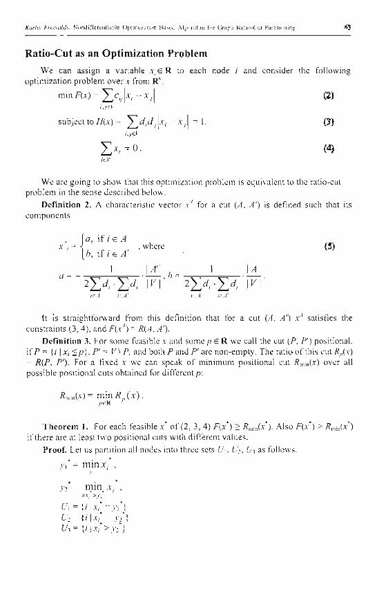
Karlis h'reivalds. Nnndif ierci i t iLtblc O p u m i / a i i u n B a s e d A k ' n r i l h m l o r G r a p h R a l i o - C u l P a r t i t i o n i n g

Ratio-Cut as an Optimization Problem

W e can assign a variable v . e R to each node i and consider the following opt imizat ion problem over x from R".

m i n F ( x ) = _^/, j|-V, ~Xj\ (2)

subject to 77(A) = ^ < 7 , C / L | A - , . - A \ | = 1. (3)

f./ef

£ * , - = f l . (4) id'

W e are going to show that this opt imizat ion problem is equivalent to the ratio-cut problem in the sense described below.

Definition 2. A characteristic vector xA for a cut (.4, A') is defined such that its componen t s

\a, i f / e A x'; = < , where (5)

[b, ifieA'

1 1 M l

in A ieA' IQA le.-f

It is s traightforward from this definition that for a cut (A, A') xA satisfies the constraints (3 , 4) , and F(xA) = R{A, A').

Definition 3. For some feasible x and some p e R we call the cut (P, 7") posit ional, if P = {/ x, <p\. P' = V\ P, and both P and 7" are non-empty . The ratio of this cut Rp(x) = R(P, 7"). For a fixed x we can speak of min imum posit ional cut Rmm(x) over all possible posi t ional cuts obtained for different p:

Rmm(x) = mmR ( a ) . pSR p

Theorem 1. For each feasible x* of (2, 3 , 4) Fix) > Riwn(x'). Also F(x') > Rnm(x') i t ' there are at least two positional cuts with different values.

Proof. Let us partition all nodes into three sets Lri. L'2, U3 as follows.

1 , ' = m i n x , . ,

v s * = m i n a", ,

64 D A T O R Z I N A T N E UN I N F O R M A C I J A S T E H N O L O G I J A S

If U:, is empty there is exactly one posit ional cut, x is in the form of characteristic vector and F(x ) = Rmm(x') that concludes this proof, o therwise define

>•;, = m i n x ,

We create a sub-prob lem of (2. 3, 4) by reducing the original one to a new variable

min F,(v) = 2 ^ c t j | y , - v, | + ^ c , ; | v , + / , - y, | + i<EU., / c i A

2> i e G . J c G ,

<4 3 ' J

subject to

H,(y) = 2 Y.d>di h " >'• I + X l / ( / . + lJ ~ >' i

ICU{ JtL'z -/'c^A

(6)

| c / , |v | + | L / - , | > S + | L / , | V , = 0 ,

where constants /, = x, - v 3 .

(7)

(8)

1

^ ; c C - , . / e C / ,

X, - I ,

Next, we further restrict it w i t h y , < v'2 < y j and can drop the absolute value signs:

min F:(y) = 2 ( y , - y , ) + ^ c / ; ( y 3 + - V,) +

^(y.+lj-y.) +K, (9)

subject to

/7<v) = 2 ^ c / , c / , ( y 2 - y , ) + > \ / t / ( v 3 • 1; v , ) •

( V ; +lj-y2) ^P=l (10)

Karlis Frcivalds. N o n d i f ' f c r c n t i a h l c O p t i m i s a t i o n B a s e d A l g o r i t h m l o r G r a p h R a l i o - C u l P a r t i t i o n i n g

V] < V'2 < > ' j .

(11)

(12)

W e have obtained a locally equivalent linear program in the sense that for v the constraints (10, 11, 12) are satisfied and F(x') = F2{\'). Also , if we can find a better solution for (9 -12) we can substi tute the result back to the original problem giving a better feasible solution for it.

From the linear p rog ramming theory it is known that we can find the optimal solution by examining the vert ices of the polytope defined by the constraints - in our case that means when one of the inequalit ies in (12) is satisfied as equali ty. Let us examine both cases:

H2 ( V | , V l . V ; , ) =

( v 3 - > • , )

= 2 ( v 3 - v , ) _idld] - I. 1. i n U ^ C . j c i : ,

.here 1 = 2 + icUilM ,JCL':,

F~2 ( v ' i , > ' i , v 3 ) = 2 ( . v 3 - v , ) _ _ > , + Z C v / , + A '

Ot/'j .yet', ' t O ' i L't/'i .ye t ' ,

By subst i tut ing vj - Vi from previous equat ion we get

f ^ O t - V , , > ' ; , ) = L / Z ' . + X ' ' - ' . '

(1 -L)R(U, U CA, tTjl + B^

where 5 = 2 + A*.

case v 2 =j'.v Similarly we get F 2 0 ' i - > : . = ( 1 - I ) /?(£/,. £A U t/.O - 5 ,

W e chose the solution y with y, = y : if /x(Lj U tA, CAJ < /?(£/,. £A IJ c ' 3 ) , otherwise choose the solution with i 2 = y 3 . It is evident that if both these ratio costs are non-equal we get a strictly smaller function value. We substi tute the solution back into the original problem obta in ing a new .v. x is a feasible solution of (2, 3. 4) with a smaller or equal function value and the set LA merged to U\ or Uj. W e repeat the described process until lA is empty .

Let us analyze the resul t ing x and sets b\ and LA We have F(x) = R(L'\, U2). where (L'i. U2) is some posit ional cut of x (in fact the minimal one) , hence Fix ) > F(x) >

66 D A T O R Z I N A T N E U N I N F O R M A C I J A S T E H N O L O G I J A S

Rm\n(.x )• It" we had some non-equal eu'.s c o m p a r e d dur ing the process, we would have a strict decrease in the function and hence the second s ta tement of the theorem holds.

D

Definition 4. A feasible x is a local m i n i m u m of (2 . 3, 4) if there exists 8 > 0 such that Fi/) < F(x) for each .v satisfying ( 3 , 4) and | ; x-x' || < e.

Definition 5. A feasible A is a strict local m i n i m u m of (2. 3 . 4) if there exists s > 0 such thai F{x ) < Fix) for each a - x satisfying ( 3 , 4) and 1 A - v* \\ < z.

T h e o r e m 2. Each strict local min imum .v of (2. 3, 4) is in the form .v* - x"1 for some cut (A. A').

Proof. W e need to prove that in a strict local m i n i m u m the expression (5) holds for some a and />. and the correct values for a and /; are guaranteed by the constraints (3) and (4). Assume to the contrary that there are more than two distinct values for the components of x . We form the reduced p rob lem as in Theo rem 1 obtaining equat ions (9 - 12). We are able to do that since L\ is non-empty due to our assumption.

From the linear p rogramming theory' a strict local m i n i m u m can only be on the vertex of the polytope d e n n e d by the constraints (10 - 12), however in our case y cannot be on the vertex since the constraints where equali ty holds at v are less then the number of variables. Consequent ly , x cannot be a strict local min imum for the original problem. Hence our assumpt ion is false and the theorem is proven.

There is one- to-one cor respondence be tween strictly locally minimal cuts and strict local min imums of (2, 3. 4) as stated in the fol lowing theorem.

T h e o r e m 3 . x is a strict local m i n i m u m of (2, 3. 4) if and only if .v is a characteristic vector of some strictly locally minimal cut (A, A').

Proof. First we prove that the character is t ic Vector xA of a strictly locally minimal cut (A, A') corresponds to a strict local m i n i m u m of (2, 3. 4) . Assume to the contrary that x is not a strict local min imum point; then by Definit ion 5 there exists an arbitrary smal l vector / ± 0 that leads to smaller or equal feasible solution ,v - .v'1 - t, F(x) <Fix'). By the nature oi the constraints (3 . 4 ) there will be at least two positional cuLs of x. and sin.ee t was sufficiently small , one of them is (A, A'). There are two cases: (i) there exists a positional cut Rp(x) with value not equal to R(A. A'). Then by

Theorem 1 there is a positional cut with value Rr(x) < Fix) < Fix') = R(A, A') which divides the nodes into sets 0", and (A. Since / was sufficiently small, both Ut

and LA cannot contain nodes from both sets A and A' i.e. either 6 ) C A. or L) C A\ or UjC A, or .'A_C A' contradicting the local minimality of (A, A') by Definition 1.

(ii) all positional cuts of.v are of the same value. Let us choose some positional cut (U,, L*:) = [A, A')- And again, since we can choose / small enough., either L\ c A, or V- C A', or LVcz A, or (A c A' which contradicts strict local optimality of (A, A'} by Definition 1.

Secondly, we prove that each strict local min imum x of (2, 3, 4) is in the form of a characteristic vector of a strictly locally minimal cut. From Theorem 2 we have that each strict local min imum is in the form of a characteristic vector A' ' 1 of some cut (A. A'). W e need to show that this cut is strictly locally minimal . Assume to the contrary that there exist S <z .•(, S 0, A \ S - 0 for which R(A \ S, A' U S) < R(A. A'). Denote U = A \ S.

Kivlis l-'rcivaLls. NiMi i i i l t crc i i l i jb lc O p u m i / a t m n B;iscd A l g o r i t h m ior G r a p h R j i j o - C u i PatUi iu imi^

Let us repeat the construct ion from the proof of Theorem 1 taking the sets Ui, U2 and U3 as 5 , U, A' correspondingly. We obtain equat ions (9 - 12) and y with v, = y2. From Definition 5 each small move increases the function. Let us take such feasible move t that does not destroy the groups L'i, U2 and L"3 but separates U\, from U2. Let /' be the projection o f / o n t o the sets i •. U2. £/ 3 i.e. /' = (/,. ke U\, tp p G L'2, tr\ r e (I,). Let us d e n o t e y " = y + / ' = y ~ at' where a is chosen such t h a t y ' ; - v L

3 . Since the constraints (10, 11) are linear and they have the same value for y and y"', they will have the same value for y ' , which is a linear combinat ion of y and v"'. Obviously y' satisfies the constraint (12). Similar arguments hold for the function: since F2(y"') > F2(y), also F:(y')> F2(y) from the linearity of (9). From v c we can go back to the original problem and obtain . y \ which is a characteristic vector of the cut {A \ S. A' [j S). Since H (x ) * / / . ( / ' ) = 1 and F{x') = F2(y) > F2(y) = R(A, A'). R(A \ S. A' U 5) > R(A. A') which contradicts our assumpt ion.

• We shall note that also for each non-strictly minimal ratio cut, its characteristic

vector x' gives a local m i n i m u m of the function, however the converse is not true. There exist non-str ict local min ima of (2, 3. 4) with the function value not equal to any locally minimal cut value. In Fig. 3 a graph and their node coordinates in a local min imum of (2, 3 , 4) arc shown. It is a local m i n i m u m because no small move gives a decreased posit ional cut or a better function value. But none of its positional cuts are locally minimal .

T h e o r e m 4. The m i n i m u m ratio-cut R is equal to the opt imum solution of (2, 3 , 4 ) .

Proof. F rom Theorem 1 F(x) > R..n..n(x) > R. For the characteristic vector x4 of the m i n i m u m ratio cut F(x':) = R. The claim follows immediate ly . •

T h e o r e m 5. Each locally minimal cut {A, A') is not greater than two t imes the m i n i m u m ratio cut.

Proof. Let us denote the optimal cut ( 5 . B'). We form four sets ADB. Af\B', A'PiB. AT\B' shown in Fig. 1 From Definition 1 the ratio of each of the cuts C\ - (ACiB, V -4 0 5 ) . C : = (AnB\ V - APiB'). C, = (AT\B\ : ;TIB') , CA = (A'DB. V - A'OB) is at least as large as ratio of C\2 = (T, A') and C 3 3 = (B. B').

W e form a full graph by taking each of the sets AHB, Af)B'. A'PiB, A'DB' as the nodes of the graph and assign edge capacit ies as the sum of all edge capacit ies in the original graph between the corresponding sets. We obtain

c\ + c 4 + c, n c, + c-, + c .

dx{d-> + + d4) d2(di - r d, - dA)

c^ + c , + c. c , - r c, + L' , R} = 5 - — . R,'

d,(dl T d2 + d4) d4(</, + d 2 - rf,)

R t l ^ ^ i 2 < L _ , fl,,-

(<:/, + d2)(dj + d4) (d2+ciy)(ci^JA)

R,>Rr. Ri>R\2. /? 3 > A ' ,2- R+>R-.i

68 D A T O R Z I N A T N E UN I N F O R M A C I J A S T E H N O L O G I J A S

Fig. L I l l u s t r a t i o n o f t h e p r o o f o f T h e o r e m 5 .

And the s ta tement of the theorem to be proven t ranslates to —— < 2 . We verified

this using symbolical computat ion in Mathemat ica 4.0. See Appendix A for details.

Corol lary 6. Each strict local m i n i m u m of (2, 3 . 4) is not greater than two times the minimum ratio cut.

The proof is s traightforward from Theorem 3 and T h e o r e m 5.

The bound of T h e o r e m 5 is tight; the graph with 4 nodes shown in Fig. 2 achieves this bound. One can m a k e larger examples easily by subst i tut ing any connected graph with sufficiently high edge capacit ies in place of the nodes of the given graph.

The Algorithm

In this section we present a heurist ic a lgor i thm based on standard nondifferentiable optimization methods for finding a local m i n i m u m of (2 , 3) . Finding the min imum of a nondifferentiable function is one of several wel l -explored nonl inear p rogramming topics [5, 23] . One of the possibil i t ies is to approximate the nondifferentiable function with a

Fig. 2. A graph achieving Fig. 3. A graph with assigned node coordinates the boundary of Theorem 5. in a local minimum of (2, 3. 4) where no

positional cut is locally minimal.

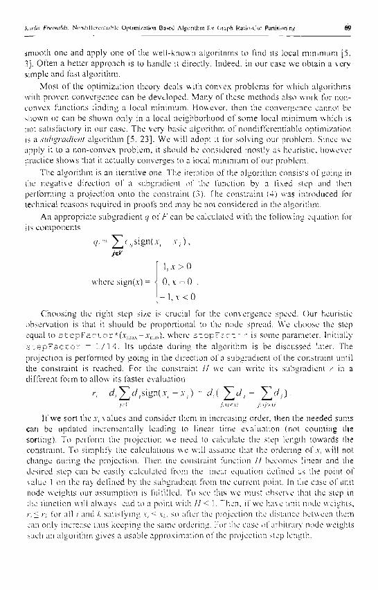
Kj/iis Frt'ivatils N n n d i t l e r c i u i a h l e O p t i m i z a t i o n Ba^cd AI^uriLhm for Graph R a t i o - C u t Part i t ioning 69

smooth one and apply one of the wel l -known algori thms to find its local m i n i m u m [5. 3]. Often a better approach is to handle it directly. Indeed, in our case we obtain a very simple and fast a lgori thm.

Most of the opt imizat ion theory deals with convex p rob lems for which algori thms with proven convergence can be developed. Many of these methods also work for non-convex functions finding a local min imum. However, then the convergence cannot be shown or can be shown only in a local neighborhood of some local m i n i m u m which is not satisfactory in our case. The very basic algorithm of nondifferentiable optimization is a subgradient a lgori thm [5. 23] . W e will adopt it for solving our problem. Since we apply it to a non-convex prob lem, it should be considered most ly as heurist ic, however practice shows that it actual ly converges to a local m i n i m u m of our problem.

The algori thm is an iterative one. The iteration of the algori thm consists of going in the negat ive direction of a subgradient of the function by a fixed step and then performing a projection on to the constraint (3). The constraint (4) was introduced for technical reasons required in proofs and may be not considered in the algori thm.

An appropriate subgradient q of F can be calculated with the following equation for its componen t s

Choos ing the right step size is crucial for the convergence speed. Our heuristic observation is that it should be proportional to the node spread. W e choose the step equal to s t e p F f - . o r * ( . r m a x - x , K m ) . where s t e p F a c t ^ r is some parameter . Initially o t e p P ' a c L o r = 1 / 1 4 . Its update dur ing the algori thm is be discussed later. The projection is performed by going in the direction of a subgradient of the constraint until the constraint is reached. For the constraint H we can write its subgradient /• in a different form to allow its faster evaluat ion

If we sort the .v, va lues and consider them in increasing order, then the needed sums can be updated incremental ly leading to linear t ime evaluat ion (not counting the sorting). To perform the projection we need to calculate the step length towards the constraint. To simplify the calculat ions we will assume that the ordering of .v, will not change dur ing the projection. Then the constraint function H becomes linear and the desired step can be easily calculated from the linear equat ion defined us the point of value 1 on the ray defined by the subgradient from the current point. In the case of unit node weights our assumpt ion is fulfilled. To see this we must observe that the step in the function will a lways lead to a point with If < 1. Then, if we have unit node weights , r, < ;> for all / and k satisfying .v, < A, ; , so after the projection the distance between them can only increase thus keeping the same ordering. For the case of arbitrary node weights such an algori thm gives a usable approximat ion of the projection step length.

1&

where sign(x)

1 , A - > 0

0,.v = 0

- 1 , * < 0

r. •,= t 7 , ^ c / / s i g n ( . T . - x . ) = d:( } - V ( / ( )

70 D A T O R Z I N A T N E L'N I N F O R M A C I J A S T E H N O L O G I J A S

The whole algori thm starts with a r andom initialization. We assign a random position for each node such that H < 1 and then perform a projection to obtain a feasible starting position. We exper imented also with several other init ial izations, but obtained significant improvements only for tree g raphs . Since the opt imal cut for trees can be found in linear t ime, we can construct a start ing posit ion that reveals it and the algorithm will only perform a few iterations to confirm that the solution does not improve. Hence to get a comprehens ive picture of the a lgor i thm behavior we decided to consider random initialization only.

After the initialization we perform iterations until convergence . To tell when the process is converged we track the m i n i m u m posit ional cut values obtained at each iteration. The same values will also tell us how to change the step size parameter s t e p F a c t o r . If the new cut value is lower than the previous one. then we are making progress and we should cont inue with the s a m e step size. If the value is higher than the previous one, then the step size is too large. If the cut does not change, then we have a clue that the process has converged. O f course we do not hurry to make decisions only from one iteration. Instead we wait for a certain number of iterations control led by the constants MA.x_OSCILLATIONS and MAX_EQUAL before making the decision. Such a delay also improves the convergence speed by a l lowing to iterate longer with a larger step size

To determine the posit ional cut value at each iteration, we proceed as follows. We consider the soiled sequence of nodes, calculate the posit ional cut in each interval between two consecutive nodes , and take the m i n i m u m one. W e can do it incremental ly on the sorted sequence in t ime 0(n r m) p rovided by the sor t ing, where m is the number of edges in the graph.

As suggested in one of the exercises in [5] , the per formance of this a lgori thm can be improved by taking the previous direct ions into account . W e add the previous direction to the current one reduced by some constant R E DU C T I ON_ F AC TO R between 0 and 1. It models a heavy ball mot ion in the presence of a force in the direction of the subgradient . In our exper iments such a modif icat ion with REDUCTION_FACTOR = 0 . 9 5 performed substantially better.

All the steps described before can be imp lemen ted to run in time 0 ( « - m). Adding the time needed for sort ing the nodes o n e iteration takes t ime 0(m - n log n). The number of iterations is hard to est imate so w e will provide exper imental data in the next sections. The constants MAX O S C I L L A T I O N S and MAX_EQUAL have the most impact on the iteration count and also on the quali ty of the obtained cut. So we must select them carefully. After some exper imenta t ion we chose MAX_EQUAL = 2 0 0 and N!AX_OSCILLATIONS - 3 0 .

a l g o r i t h m ra~io-cut calculate a ran.co:ri feasible initial position acam - 0 osci 1 la uioo.Countor = 0 equalityCounter = 0 stepFactor = 1/14 w h i l e (equalit-yCounter < MAX E Q U A L !

Karlis r'rt'ivdlds. NondilTercniuhlc O p t i m i z a t i o n B a s e d A l g u n i h m tor Graph RaMi>-OiL Ptetitipning 7 1

X = x -- ' acu~ - scam * REjU-JTIO'." FACTOR + d

if (minimum positional cot value has incrioses : r. this i t e r a t i o n )

e q u a l i t y C c u n t e r = 0 o s c i l l a t i c n C o u n t e r ++

or else (minimum p o s i t i o n a l cut v a l u e has decreased in :'r.:.s i t e r a t i i r . )

e q u a l i t y C c u n t e r = • or else

e q u a l i t y C o u n t e r +4

if ( o s c i l l a t i o n C o u n t e r > M & X J 3 S C I L L A T I O N 5 ) s t e p F a c t o r / = 1 . 3 o s c i l l a t i o n C o u n t e r = 0

endwhile end

function d i r e c t i o n (x) d = subgrad ien t (x) s t e p = {•/... ... - x.. _.,) * s t e p F a c t o r x. = x + d * s t e p x ; = p r o j e c t i o n of x or. t h e c o n s t r a i n t return x

end

The Data

We evaluated the proposed algori thm on three families of graphs: random cubic graphs , random geometr ic graphs and random trees. We considered only graphs with unit weight nodes and edges.

Random cubic graphs are potentially hard for ratio-cut a lgor i thms, because in [11] it was shown that there is actually an 0 ( l o g n) gap between the min imum ratio-cut and the m a x i m u m concurrent flow on these graphs . We generate them using the algorithm provided in [14].

R a n d o m geometr ic graphs are s tandard test suite for balanced cut problems used in several papers [9, 22] , To generate a geometr ic graph we place the nodes of the graph randomly in the unit square. Then we include an edge be tween each of two nodes that are within distance 6 in the graph, where <5 is the minimum value such that the resulting graph is connected.

Tree graphs are seemingly easy graphs because their optimal ralio-cul can be calculated in linear time. Also it is not hard to show that only one local m i n i m u m exists for the corresponding opt imizat ion problem. Nevertheless , it is an interest ing family since our exper iments indicate a slow convergence of our algorithm on these graphs. Also, we can compare our result with the optimal one. We generate random trees with the classical algori thm, where each tree is produced with the same probabil i ty. This

72 D A T O R Z I N A T N E UN I N F O R M A C I J A S T E H N O L O G I J A S

algorithm produces long and skinny trees, which are part icularly difficult for our algorithm.

Experimental Results

We implemented the algorithm in and evaluated its performance on a computer equipped with a Pentium III 800 M H z processor and 256 Mbytes of R A M . For each graph family vve measured the runn ing t ime in seconds, the number of iterations and the quality of the produced cuts . Since we did not know the exact cut values for random and geometr ic graphs, we evaluated h o w much the ratio-cut value decreases when we continue the a lgor i thm for the s ame number of iterations as performed before termination. Measur ing the decrease of the ratio-cut value we can est imate how far the result is from the opt imal .

The algori thm was run on a series of g raphs of exponent ia l ly increasing size from 100 up to 204800 nodes . Ten graphs were genera ted for each size and the results were averaged. The average node degree for all graph families is constant. Al though we cannot specify the degree explicitly for geomet r i c graphs , due to their nature it was about 10 on all instances. The exper imental results are given in tables 1-3. For each graph size tables show the iteration count, the running t ime, the obtained ratio-cut value and the improved ratio-cut value when the iteration count is doubled. For tree graphs the optimal ratio-cut value is shown also. Let us d iscuss the results separately for each graph family.

Cubic Graphs

Although these graphs were suggested as difficult, the algori thm performed very well on them. It took on average about 35 minutes to parti t ion the 204800 node graphs. The running t ime dependence on the graph s ize is shown in Fig. 4. When we approximated the running time with a function in a form 0(rr") we get the asymptot ical running t ime about 0{nb) on these graphs.

The algori thm seems to find a very close to opt imal cut since after doubl ing the iteration count, the quali ty increased only by less than 0 .4%. Even more, the quality improved for the larger graphs approaching 1 (see Fig. 7). Such behavior is not surprising since it is not hard to prove that the rat io of a cut (A, A') of a r andom cubic

graph is on average independent ly of the sizes of A and A' (a similar proof for n -1

general r andom graphs is presented in [20]). Then it is unl ikely that the min imum ratio cut will be much different from this average value.

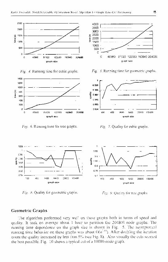
Kitrlis f-reivalds. N o n d i t ' t c r e n l i a b l c O p t i m i z a t i o n B a s e d A l g o r i t h m to r G r a p h R a l i o - C u l P a r t j i i u n i n y 73

8 1 9 2 0 1 2 2 8 8 0 163840 2 0 * 3 0 0

g r a p h s i ze

4000

3 5 0 0

3000

2500

2000

1500

1000

500 \

0

0 4 0 9 6 0 81920 122880 163840 204800

g r a p h s ize

Fig. 4. Running time for cubic graphs. Fig. 5. Running time for geometric graphs.

0 4 0 9 6 0 8 1 9 2 0 1 2 2 8 8 0 163843 2 0 4 8 0 0

g r a p h s ize

tflfj 4O0 1603 64 X 2 5 6 0 0 102400

g r a p h size

Fig. 6. Running time for tree graphs. Pig. 7. Quality for cubic graphs.

1.01 ,

0 94 1 ;

100 400 1600 6 4 0 0 25600 102400

g r a p h s ize

Fig. iV . Quality for geometric graphs.

0.75 i

0 7 ,

100 4 0 0 1600 6400 2 5 6 0 0 102400

g r a p h size

Fig. 9. Quality for tree graphs

Geometric Graphs

The algor i thm performed very well on these graphs both in terms of speed and quality. It took on average abotit 1 hour to partition the 204800 node graphs . The running t ime dependence on the graph size is shown in Fig. 5. The asymptotical running t ime behavior on these graphs was about Q ( « A f t e r doubl ing the iteration count the quality increased by less than (see Fig. 8). A l so visually the cuts seemed the best possible. Fig. 10 shows a typical cut of a 10000-node graph.

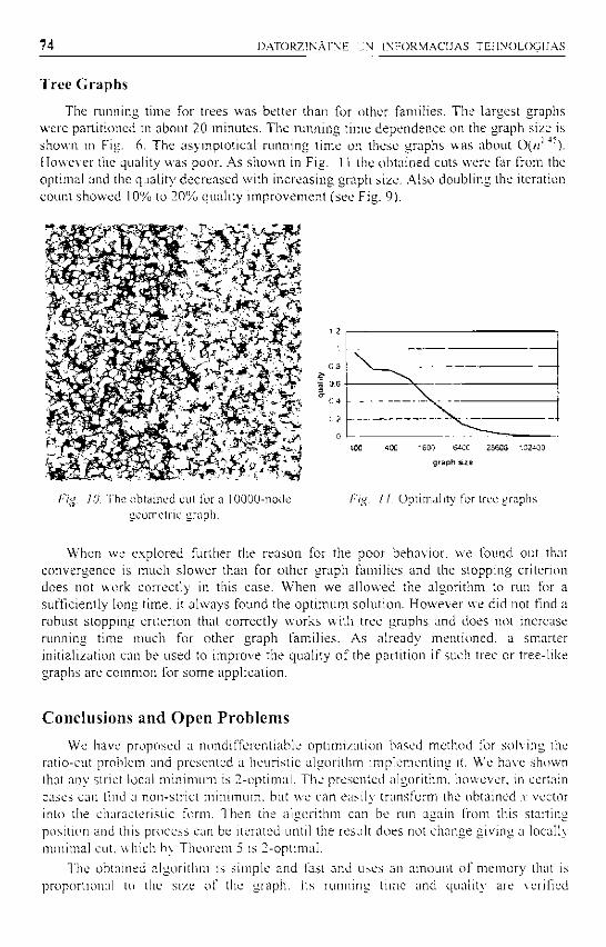
74 D A T O R Z I N A T N E E N I N F O R M A C I J A S T E H N O L O G I J A S

Tree Graphs

The running time for trees was better than for other families. The largest graphs were part i t ioned in about 20 minutes. T h e running t ime dependence on the graph size is shown m Fig. 6. The asymptot ica l running t ime on these graphs was about 0(n] 45). However the quality was poor. As shown in Fig. 1 1 the obtained cuts were far from the optimal and the quality decreased with increasing graph size. Also doubl ing the iteration count showed 10% to 2 0 % quality improvement (see Fig. 9) .

Fig, 10. The obtained cut for a 10000-node Fig. 11. Optimality for tree graphs geometric graph.

When we explored further the reason for the poor behavior , we found out that convergence is much s lower than for other graph families and the s topping criterion does not work correctly in this case. When we a l lowed the algori thm to run for a sufficiently long t ime, it a lways found the o p t i m u m solution. However we did not find a robust s topping criterion that correctly works with tree graphs and does not increase running time much for other graph families. As already ment ioned, a smarter initialization can be used to improve the qual i ty of the parti t ion if such tree or tree-like graphs are common for some application.

Conclusions and Open Problems

We have proposed a nondifferentiable opt imizat ion based method for solving the ratio-cut problem and presented a heurist ic a lgor i thm implement ing it. W e have shown that any strict local m i n i m u m is 2-opt imal . The presented algori thm, however , in certain cases can find a non-str ict m in imum, but we can easily transform the obtained .v vector into the characterist ic form. Then the a lgor i thm can be run again from this starting position and this process can be iterated until the result does not change giving a locally minimal cut. which by Theorem 5 is 2-optimal .

The obtained a lgor i thm is s imple and fast and uses an amount of m e m o r y that is proportional to the size of the graph. Its running t ime and quality are verified

Karlis I-reivahts. N i m d i f i c r e n l i a b l c O p t i m i z a t i o n B a s e d A l g o r i t h m tor Graph R a l i o - C u l Part i t ioning 75

experimental ly. Its practical running t ime is about 0(n)t') on our test data. The algorithm produces high quali ty cuts on random cubic and geometr ic graphs. On trees and other very sparse graphs the quality can be significantly improved by choosing a better starting position than a random one. We evaluated the algorithm on artificially generated data. As further s tudy it would be important to evaluate its performance on real-life problems.

Although the algori thm performed well on most graphs,, it is heuristic anyway. Is it an open question whether we can find a local min imum of (2 . 3 , 4) in polynomial time?

Acknowledgements

The author would like to thank Paulis Kikusts and Krists Boi tmanis for valuable discussion and help in preparat ion of this paper.

References

1. C. J. Alpert and A. Kahng. Recent Directions in Netlist Partitioning: a Survey. Tech. Report, Computer Science Department. University of California at Los Angeles. 1995.

2. C. J. Alpert, J.-H. Huang, and A. B. Kahng. Multilevel circuit partitioning. Proc. Design Automation Conf, pp. 530 533, 1997.

3. R. Baldick. A. B. Kahng, A. Kennings and T. L. Markov. Function Smoothing with Applications to VLSI Layout, Proc. Asia and South Pacific Design Automation Conf., Jan. 1999.

4. J. W. Bern,' and M. K. Goldberg. Path Optimization for Graph Partitioning Problems. Technical report TR: 95-34, DiMAC'S, 1995.

5. D. Bertsekas. Nonlinear Programming. Athena Scientific. 1 999. 6. L. Hagen and A. B. Kahng. New Spectral Methods for Ratio Cut Partitioning and Clustering.

IEEE Trans. Computer-Aided Design. 1 1 (1992). pp. 1074 1085. 7. T. Hamada. C.-K. Cheng. P. M. Chau. An Efficient Multilevel Placement Technique using

Hierarchical Partitioning. IEEE Trans, on Circuits and Systems, vol. 39(6) pp. 432 439. June 1992.

8. P. Klein. S. Plotkin, C. Stein, E. Tardos. Faster Approximation Algorithms for Unit Capacity Concurrent Flow Problems with Applications to Routing and Sparsest Cuts. SIA.M J Computing. 3(231(1994). pp. 466-488.

'•). K. Lang and S. Rao. Finding Near-Optimal Cuts: An Empirical Evaluation. 4th. ACXf-SIAM Svmposium on Discrete Algorithms, pp. 2 1 2 -221. 1993.

10. T. Leighton. F. Makcdon. S. Plotkin, C. Stein. E. Tardos, S. Tragoudas. Fast Approximation Algorithms for Multicommodity Flow Problems. Journal of Computer and System Sciences. 50(2), pp. 228-243. April 1995.

11. T. Leighton. S. Rao. Multicommodity Max-Flow Min-Cut Theorems and their use in Designing Approximation Algorithms. Journal of the ACM. vol 46 . No. 6 (Now 1999), pp. 787 • 832.

12. T. Lengauer. Combinatorial Algorithms for Integrated Circuit Layout. Stuttgart. John Wiley & Sons 1 994.

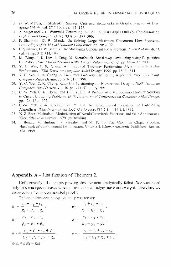
76 D A T O R Z I N A T N E UN I N F O R M A C I J A S T E H N O L O G I J A S

13. D. W. Matula, F. Shahrokhi. Sparsest Cuts and Bottlenecks in Graphs. Journal of Disc. Applied Math., vol. 27 (1990). pp. 113 123.

14. A. Steger and X. C. Wormald. Generating Random Regular Graphs Quickly. Combinatorics, Probah. and Comput. vol. S (1999). pp. 377 396.

15. F. Shahrokhi, D. W. Matula. On Solving Large Maximum Concurrent Flow Problems. Proceedings of ACM 1987 National Conference, pp. 205-209.

16. F. Shahroki, D. W. Manila. The Maximum Concurrent Flow Problem. Journal of the ACM, vol. 37. pp. 3 IS 334. 1990.

17. M. Wang, S. K. Lim, J. Cong, M. Sarrafzadeh. Multi-way Partitioning using Bi-partition I leuristics. Proc. Asia and South Pacific Design Automation Conf. pp. 667-672. 2000.

18. Y. C. Wei, C. K. Cheng. An Improved Two-way Partitioning Algorithm with Stable Performance, IEEE Trans, on Computer-Aided Design, 1990, pp. 1502-1511.

19. Y. C. Wei. C. K. Cheng. A Two-level Two-way Partitioning Algorithm. Proc. lnt'l. Conf Computer-Aided Design, pp. 516-519. 1990.

20. Y. C. Wei. C. K. Cheng. Ratio Cut Partitioning for Hierarchical Designs. IEEE Trans, on Computer-Aided Design, vol. 10. pp. 9 i 1 -92 I. July 1991.

21. C.-W. Yeh. C.-K. Cheng, and T.-T. Y. Lin. A Probabilistic Multicommodity-flow Solution to Circuit Clustering Problems. IEEE International Conference on Computer-Aided Design. pp. 428 4 3 1 , 1992."

22. C.-W. Yeh. C.-K. Cheng, T.-T. Y. Lin. An Experimental Evaluation of Partitioning Algorithms. IEEE International ASIC Conference. PI4-I . I - P14-14: 1991.

23. X. Z. Shor. Methods of Minimization of Nondifferentiable Functions and their Applications. Kiev, "Naukova Dumka" 1979. (in Russian).

24. I. Bomze, M. Budinich. P. Pardalos, and M. Pclillo. The Maximum Clique Problem. Handbook of Combinatorial Optimization, Volume 4. Kluwer Academic Publishers. Boston, MA, 1999.

Appendix A - J u s t i f i c a t i o n o f T h e o r e m 2.

Unfortunately all a t tempts proving this theorem analytical ly failed. W e succeeded only in some special cases when all nodes or all edges have unit weight . Therefore we resorted to a '"computer assisted p r o o f .

The equali t ies can be eqtuvalently writ ten as:

c, + c, +c, c, — c\ + c-

A'i/n'.-.v Frftvalds. N o n d i r i e r c n l i a h l c O p l i r m / i i i i o n B a s e d A l ^ i i n l h m lor Graph R a l i o - C u l P a v i l i o n i n g 77

A, >Rtl, R2>R\z- A'; ' A' .-. • A'- .

prove:

Since all the inequali t ies do not change when we multiply all c. with some constant , we can choose this constant such, that R]2 = I- Solving this equality for c ; and substi tuting the result into the inequalities we obtain. ( l iven:

This is the s ame as p rov ing that (1)—(5) together with the negation of (6) can never be satisfied for any values of the involved variables. Let us also remember that the variables come from node weights and edge capacit ies that are nonneganve . W e can further require that g, are strictly positive; in the opposite case the proof is easy. W e verified that these inequalit ies have no solution with several numerical solvers, however that does not guarantee the correctness due to numerical errors. Therefore we used the Cylindrical Algebra ic Decomposi t ion method implemented in Mathemat ics 4.0 to verify the inequalit ies using symbolic computat ion. The running time of the Cylindrical Algebraic Decomposi t ion algori thm is inherently doubly exponent ia l : hence we had to transform the inequali t ies and write support ing functions to obtain results in practically reasonable t ime. Using symbol ic computat ion we can be certain, if Mathemat ica has no implementat ion bugs, our conjecture holds.

The Mathemat ica 4.0 no tebook to verify these inequalities follows.

(.1)

gs - g(, > 0

78 D A T O R Z I N A T N E : I N I N F O R M A C U A S T E H N O L O C I J A S

(ri[11 = ( v We i n t r o d u c e a u x i l a r y f u n c t i o n t o s p e e d u p t h e c a l c u l a t i o n s . 1 1

r e t u r n s F a l s e i f a n d o n l y i f t h e e x p r e s s i o n i s a l w a y s f a l s e * )

V e r i f y [ a _ | | b ] : = ( E x a m i n e [ a ] || V e r i f y [ O r [ b ] ] ) ;

V e r i f y [ a ] : = E x a m i n e [ a ] ;

E x a m i n e [ a ] : = E x p e r i m e n t a l C y l i n d r i c a l J S V l g e b r a i c D e c o m p o s i t i o n [

a , ( g l , g2 , g 3 , g 4 , g 5 , g6, c 5 , c 6 , c l , c 3 , c 4 } ] ;

$ E . e c u r s i o n l i m i t = 1 0 0 0 0 ;

e q l ^ c l * c 4 + c 6 - g l - g 4 - g 6 ;

e q 2 - c l - c 4 - c 6 - g l + g 4 +• g 6 ;

e q 3 E c 3 - c 4 - c 5 - g 3 * g 4 + g5 ; e q 4 - c 3 + c 4 + c 5 - g 3 - g 4 - g5 ; e q i m j i = 2 ( c l + c 3 *• c 5 + c G ) - g l - g 3 - g.5 - g 6 ;

(w Do t h e v e r i f i c a t i o n i n t w o s t e p s . D o i n g i t a l l t o g e t h e r

t a k e s t o o m u c h t i m e *•)

t m p R e s u l t = E x p e r i m e n t a l " C y l i n d r i c a l A l g e b r a i c D e c o m p o s i t i o n [

c 5 >= 0&& c 6 > = 0 S & e q 2 > = 0 && e q 4 > = 0 && e q l > = 0 && e q 3 >= 0 &&

e q i m p < 0 g l > 0 g3 > 0 && g 5 > 0 ,

{ c 5 , c 6 , g l , g 2 , g 3 , g 4 , g 5 , g 6 , c l , c 3 y c 4 } ] ;

V e r i f y [ L o g i c a l E x p a n d [ t m p R e s u l t g l w g 3 — g 2 * g 4 == g5 * g 6 ] ]

0Ji\]"= F a l s e

Table I. Exper imenta l results for tree graphs .

Node count

Iterations Time (s) Cut value Improved cut Optimal cut

100 257 0.01755 0.000424058 0.000421019 0.000407809 200 377 0.05105 0.000131803 0.00010598 0.000101407 400 512 0.1377 3.38841 E-05 3.14657E-05 2.55342E-05 800 739 0.43965 9.62S36E-06 7.94314E-06 6.32I58E-06

1600 906 1.14515 3.49721E-06 3.10424E-O6 1.58787E-06 3200 987 2.72245 1.3683E-06 1.14917E-06 3.97123E-07 6400 1085 8.336 7.15262E-07 5.51447E-07 9.884S5E-08

12800 1294 27.96925 3.34456E-07 2.98915E-07 2.46653E-08 25600 1343 79.48075 1.78731 E-07 1.59801 E-07 6.19941E-09 5 1200 1374 199.9305 1.031S7E-07 9.352E-08 1.53453E-09

102400 1115 359.242b 6.66622E-0S 6.17942 E-08 3.89972E-I0 204800 1734 1197.7344 2.S1771E-08 2.60658E-08 9.6445E-I I

Ktirlis i'reivtdds. N o n d t f l c r c n l i a h l c O p t i m i z a t i o n B a s e d A l g o r i t h m for G r a p h R a i i o - C u i Pa r i i t i nn in - j

Table 2. Experimental results for cubic graphs .

Node count Iteration count Time (s) Cut value Improved cut 100 199 0.013 0.005185495 0.005166088 200 290 0.04205 0.002513133 0.002510172 400 383 0.11065 0.001214463 0.001213595 800 570 0.36905 0.0005994 0.000598147

1600 727 1.02045 0.000296 0.000295773 3200 835 2.69475 0.000147637 0.000147552 6400 1012 8.92785 7.36747E-05 7.36234E-05

12800 1 195 30.71865 3.67635E-05 3.675E-05 25600 1455 107.70535 1.8375E-05 1.83679E-05 51200 1672 320.36415 9.15616E-06 9.15434E-06

102400 1998 834.6924 4.56971E-06 4.56927E-06 204800 2500 2254.4636 2.28649E-06 2.28627E-06

Table 3. Exper imenta l results for geometric graphs .

Node count Iteration count Time (s) Cut value Improved cut 100 129 0.016 0.002848427 0.002845499 200 146 0.04305 0.001631237 0.001620948 400 204 0.1282 0.000592549 0.0005825 800 266 0.4532 0.000338845 0.000333014

1600 389 1.9732 0.0001 16216 0.000113355 3200 430 5.28105 5.88979E-05 5.82837E-05 6400 530 14.3365 2.34042E-05 2.25542E-05

12800 681 45.96155 1.13718E-05 1.09091E-05 25600 800 149.0739 5.18003E-06 5.18003E-06 51200 886 461.85255 2.88345E-06 2.88345E-06

102400 976 1 169.0154 1.4I57E-06 1.4157E-06 204800 1417 3797.3582 3.32351E-07 3.14612E-07

L A T V I J A S U N1V E R SI T A T E S R A K S T 1 . 2 0 0 4 . 6 6 9 . s e j . : D A T O R Z I N A T N E U N I N F O R M A C I J A S T E H N O L O G I J A S . t O 88. l P p .

Review of Traceability Models for Software Testing Processes

Martins Gills Riga Information Techno logy Institute

Kuldigas i e l a 4 5 , Riga. L V - 1 0 8 3 . Latvia martins.gil ls(a ; r i t i . lv

A considerable part of software development activities is devoted to testing. The scale of testing may depend on quality criteria for the particular development project. As soon as development and testing is performed in some organized manner, there exist some relations and dependencies between all types of project items. The relations outline some path of traceability that starts from the origins of a particular item, and follows to its derivatives in a form of other item types. This paper reviews various traceability models for software projects, and analyses the sub-models of testing processes. The common properties of these models arc identified. Key words: traceability, problem reporting, testing process.

Introduction

The property of traceability for software development projects has been known for long. It usually assures a better control over software development artefacts, provides a more organized project life-cycle and. consequently, reduces the risk of developing a low quality product [6], Testing as one of software processes is extensively dependent on the established traceability principles or. more formally, a traceability model within the given project. A vital problem in software testing is to establish an appropriate coverage of requirements. Typically, the formal coverage could be achieved according to some criteria, e.g. stating that each requirement must have at least one appropriate test, or in more advanced situations using standard requirements like ones of BS 7925-2 [3j . It is especially important to evaluate the impacts of requirement 's changes or to analyse the updates within the test suite. The previously mentioned issues are related to traceability property within the software development life cycle and to the testing process in particular.

Software testing process properties

A large part of the effort devoted to software development is due to software testing [11]. Software testing can be regarded as one of the processes presenting within any software development life cycle. Although it may not appear explicitly within the formal list of processes (like e.g. in ISO/IEC 12207 [8]). it may be derived as a tailored process.

Typically, the testing is organized at various levels, depending on what is the focus of the specific testing activity. The concept of test levels (test activities with a common direction) is mainly derived from the software development V-model. The model itself originally comes from the Software Lifecycle Process Model [4], more often it is represented in a very simplified form [10], and as a more generic model is shown in F ig . l . In principle, the V-model is close to the more classical Waterfall software development model [11]. Every project has a different testing process, and not all projects do have tasks corresponding to

Marlins Gills. R e v i e w of T r a c e a b i l i t y M o d e l s for S o f t w a r e Tes t ing P r o c e s s e s 81

every test level - some may have very specific ones. Main differences can be due to different naming and due to the combination or subdivision of particular test levels. In each case various organizational and methodological issues play a role in defining the way these test levels are implemented. For example, a unit test may be called a component test, but acceptance testing may be subdivided as factory acceptance testing and user acceptance testing, or this level may be supplemented by qualification testing. Every test level has a different object to be tested, and the tests themselves are based on different project artefacts.

R e q u i r e m e n t s A c c e p t a n c e Tes t ing

S p e c i f i c a t i o n S y s t e m l e s t i n g S p e c i f i c a t i o n S y s t e m l e s t i n g

A r c h i t e c t u r a l .s I n t e g r a t i o n D e s i g n > T e s t i n g

\ / / Deta i l ed Des ign Uni t T e s t i n g De ta i l ed Des ign Uni t T e s t i n g

\ / /

C o d i n g - > o n the bas is of

Figure /. The V-model.

The Author has found out that in rare cases the projects can immediately say what kind of life cycle model they use. In most cases such a model exists, but it is not formally described in an explicit form, rather it is hidden within the project plan, procedures or standards. Although the notion of test levels is explicitly used in the V-model. they can be a part of other models as well. It could be extremely difficult to indicate a development process where testing is just a once-through activity with only one testing level. Even the simplest approach of quality requires a product (e.g. software element) checking activity prior to passing it further for integration into a larger product or prior to delivery. As the typical software development consists of numerous developers, project stages (typically, with cycles), there are at least two test levels present.

Traceability models for development process

According to the concept of the traceability model [5]. it is formed from project items and relations between them. The most convenient form of representation is graphical where boxes are item types and arrows indicate relations. To analyse the testing process items, the author compiled preliminary information from 14 projects. Each of those represented a slightly different development approach, but at the same time, each project from this group could be mapped to the typical life cycle building blocks defined by the standard J-STD-016 [7]. For this paper, four different models were selected, each representing some possible class of traceability models. Three of them represent custom information system development projects, and one represents development of small utility software.

Project A (see Fig.2A) represents the most popular class of traceability relations. Formal requirements are derived from customer proposals, tests are based on these requirements,

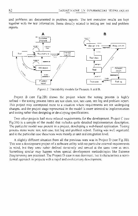
82 D A T O R Z I N A T N E U N I N F O R M A C U A S T E H N O L O G I J A S

and problems are documented in problem reports. The test execution results are kept together with the test information. Items directly related to testing are: test and problem reports.

B

C h a n g e r e q u e s t

D e s i g n i t e m R e q u i r e m e n t D e s i g n i t e m implements

R e q u i r e m e n t

T e s t P r o b l e m

r e p o r t

A described ki j

V T e s t c a s e

execution ol T e s t l og

Figure 2. Traceability models for Projects A and B.

Project B (see Fig.2B) shows the project where the testing process is highly refined — the testing process items are test class, test, test case, test log and problem report. This project may correspond more to a situation where requirements are not undergoing changes, and the project stage represented in the model is more oriented to implementation and testing rather than designing or developing specifications.

Two other projects had more relaxed requirements for the development. Project C (see Fig.3A) is a sample of the model that includes quite detailed implementation description. The particular model was present in a project, developing a web-based application. Testing process items were: test, test case, test log and problem report. Testing was well organized, and in the particular case these tests were most ly at unit and integration level.

A slightly different situation from all the previous ones was in Project D (see Fig.3B). This was a development project of a software utility with no particular external requirements in mind, but they were rather defined iteratively and served at the same time as tests. Something similar may happen when special development methodologies like Extreme Programming are practiced. Tire Project D case is not dominant, but it characterizes a semi-formal approach in projects with a rapid and evolutionary development.

Martins Gills. R e v i e w o f T r a c e a b i l i t y M o d e l s for S o f t w a r e Tes t i ng P r o c e s s e s 83

Figure 3. Traceability models for Projects C and D.

The Author found out that it was possible to map the traceability models of all 14 reviewed projects to the four models previously presented. The main difference could be that specific names are given for particular item types in each particular project. For example, requirement could be a particular diagram, use case, scenario, instruction, feature, etc.

Typical item types of testing process

The identification of testing items within the development process traceability model allows defining the traceability for the testing process. The typical constituents of the testing process are project i tems shown in Table 1.

Table I. Testing-related project i tems.

Test A set of objectives, methods and criteria to be applied in verification/checking purposes to a certain software item.

Test case A set of inputs, execution preconditions, and expected outcomes developed for a particular test objective. In some cases the test case may be created in the form of a test script for automated tests.

Test class A set of tests with similar test objectives, methods or test levels. Test configuration A set of additional test attributes to be applied during execution

for certain test cases. Test suite A set of test cases to be executed within a certain test session,

scenario or by the particular personnel. Test suite can be implemented in the form of a test script for automated tests.

Test log record Information about the status of test execution. Problem report A detailed description of test incidents, a record describing all

events requiring an additional exploration.

The identification of testing process items within project traceability models shows that the relations between these items are not random. There are typical directions of dependencies. In every project, the testing process items form some subset of a more generalized model. Figure 4 shows a generalized model of the testing process. Each individual project m a y include a subset of these, or define some specific additional testing-

84 D A T O R Z I N A T N E UN I N F O R M A C U A S T E H N O L O G I J A S

related items. For example, the test script as an item type can be added to the model for projects with a high level of test automation.

Test Test class Test b e i o r g s to

Test class

t ^ is pa r i of

Test case conta ins

Test suite Test case ^ Test suite

marks execut ion of

1 ; Test log Test record is execu ted wi th configuration

marfcs p rob lem in Problem

report

Figure 4. A generalized traceability model for testing process.

Items shown on the left side (Fig. 4) represent the typical constituents of the information set for testing that could be derived from software engineering standards like J-STD-016 [7]. The information set of the testing process has to provide answers to the following three question areas that are vital for project management and product quality:

• what is to be (or was) tested and how?

• when and how were the tests executed?

• what problems are encountered?

In Fig. 4, the project items on the right side do have a more classifying role - in some cases they could not be regarded as separate items but rather as attributes to the project items on the left side.

The most common approach in industrial projects is not to distinguish between tests and test cases. All are called tests, and the i tem could be either very detailed (like the test case), or it could outline jus t the main issues (like the test). S o m e other optimisations could take place, sometimes reducing the minimal test item set to only two project item types. Fig. 5 shows two possible cases that were observed in the projects. In case (a) there are separate tests defined, but all testing results are maintained as one log. This can function in small teams where it is not important to establish a formalized communicat ion between testers and developers, but at the same t ime testers recognize the need to document the progress and problems. Case (b) formalizes the situation in which attention is paid mainly to problem registering, and probably tests are not even in every case formally documented, but rather briefly described while they are executed. This may be typical for larger project teams than in case (a).

a) Test b) Test & execution info

marks execu t i on ot descr ibes p r o b l e m of

Resul ts of test ing (including Pr.Rep.) Prob lem report

Figure 5. Possible optimisations of traceability models of the testing process.

Martins Gills. R e v i e w of T r a c e a b i l i t y M o d e l s for S o f t w a r e Tes t ing P r o c e s s e s 85

I n s o m e p r o j e c t s , i n t e n t i o n s h a v e b e e n s e e n t o o m i t w r i t i n g t h e t e s t s , o r t e s t s a r e w r i t t e n

a s a n e x a c t c o p y o f r e q u i r e m e n t s l i s t w i t h w o r d s l i k e " m a k e s u r e t h a t " , " c h e c k " o r " v e r i f y "

a d d e d . S o m e t i m e s t h e m a i n m o t i v a t i o n f o r t h i s i s t h e n e e d t o m i n u n i z e t h e e f f o r t s p e n t o n

d o c u m e n t i n g ( d u e t o e c o n o m y r e a s o n s ) . T h i s f o r m a l i s m i s q u i t e w i d e s p r e a d i n s o f t w a r e

e n g i n e e r i n g , i t a s s u r e s a g o o d t r a c e a b i l i t y , b u t i t i s n o t e f f i c i e n t i n t e r m s o f g o o d t e s t i n g [1].

T h e O v e r a l l e v a l u a t i o n s h o w s t h a t t h e b a s e e l e m e n t , t h e i t e m t y p e f o r t e s t - r e l a t e d p r o j e c t

i t e m s i s t h e T e s t - i t h a s t o b e p r e s e n t i n t h e p r o j e c t i f t h e t e s t i n g i s m a d e . A l l o t h e r t e s t i n g

p r o c e s s i t e m s m a i n l y d e p e n d o n t h i s . T h e d e p e n d e n c e o f t h e t e s t o n t h e p r o b l e m r e p o r t d o e s

n o t p l a y a s i g n i f i c a n t r o l e - i t i n d i c a t e s t h e c a s e w h e r e n e w t e s t s m a y b e a d d e d a s a r e s u l t o f

f o u n d p r o b l e m s .

External relations of testing process items

T h e P r e v i o u s c h a p t e r d e f i n e d t h e g e n e r a l i z e d t r a c e a b i l i t y m o d e l f o r t e s t i n g p r o c e s s . A t

l e a s t t w o i t e m s - t h e t e s t a n d t h e p r o b l e m r e p o r t - w i t h i n t h i s m o d e l h a v e r e l a t i o n s w i t h

p r o j e c t i t e m s t h a t a r e n o t p a r t o f t h e t e s t i n g p r o c e s s .

Dependencies of the test

I t e m s e x t e r n a l l y d i r e c t l y r e l a t e d t o t h e t e s t ( r e l a t i v e t o t h e t e s t i n g p r o c e s s ) c a n b e

c l a s s i f i e d i n t o t h r e e g r o u p s :

• s o f t w a r e s y s t e m d e f i n i n g i t e m s ( r e q u i r e m e n t s , d e s i g n i t e m s ) ,

• t h e c o d e ,

• c o - p r o d u c t s ( e . g . u s e r ' s m a n u a l ) .

T h e t e s t i s u s u a l l y s t r o n g l y d e p e n d e n t o n t h e s e i t e m s . T h e r e i s a c o r r e l a t i o n b e t w e e n t e s t

l e v e l s a n d t h e d e p e n d e n c i e s o f t h e t e s t ( s e e T a b l e 3 ) . T h e t e s t c a n a l s o b e d e r i v e d f r o m t h e

p r o b l e m r e p o r t ( s e e F i g . 4 ) , b u t t h i s i s n o t d e p e n d e n t o n t h e t e s t l e v e l , r a t h e r o n t e s t p r o c e s s

o r g a n i z a t i o n .

T h e r e l a t i o n t o t h e i n i t i a l o r r e f i n e d r e q u i r e m e n t c o u l d b e c o n s i d e r e d a s a n o r m f o r

f u n c t i o n a l t e s t i n g . T h i s p r o v i d e s i n t h e m o s t d i r e c t w a y t h e a n s w e r t o t h e q u e s t i o n w h e t h e r

t h e e x p e c t a t i o n s o f t h e c u s t o m e r a r e m e t . D e s i g n i t e m s a n d c o d e e l e m e n t s a r e r e f e r e n c e d

p r i m a r i l y i n d e v e l o p e r t e s t s , b e c a u s e i n a t r a d i t i o n a l s e t t i n g n e i t h e r u s e r s n o r i n d e p e n d e n t

t e s t e r s w o u l d h a v e t h e a v a i l a b i l i t y t o e x p l o i t i n t e r n a l d e v e l o p m e n t i n f o r m a t i o n .

Table 3. Items related to the test and the corresponding test levels.

Project item Test levels Initial requirement acceptance Requirement system Design item integration Code element unit User's manual system, acceptance Problem report unit, integration, system, acceptance

86 D A T O R Z I N A T N E U N I N F O R M A C U A S T E H N O L O G I J A S

The relation of the test to the user 's manual is quite interesting. It could be applied in two cases - either when the documentation is under test, or when there are no formally specified requirements. Of course, there may be some defined requirements, but at the time of testing they are completely outdated, and there is no practical feasibility to base the test on these requirements. An interesting alternative approach with case studies has been proposed - to use the user ' s manual as a requirements specification [2]. Such an approach requires systematic writing of the manual, but for m a n y real-life projects this method could be less expensive than writing and maintaining two documents . A Special advantage is gained when the customer does not request these two. Relation with a problem report is typical for the tests added during the test execution phase to check the problem areas in later testing cycles.

Relations of the problem report

The problem report is an event-provoked item, and therefore it is tied with a weak relation to other items - no changes in other related items can provoke change into the problem report itself. The problem report can be related to almost any project item, but the most typical are the same as for the test. It may have numerous indirect relations (e.g. through an interface element problem it m a y point to some specific requirement). The existence of particular direct relations depends on the test level (see Table 4). In each particular project, only part of the above mentioned items are usually used. The problem report's relation to the test or test log indicates what kind activity led to the given problem report. Design, code, interface elements or the user 's manual or do indicate the location of the problem observable by the tester. Reference to the requirement could be used either to indicate problem in requirements or into its derivatives.

Table 4. Items related to the problem report and the corresponding test levels.

Project item Test levels Test unit, integration, system, acceptance Test log record unit, integration, system, acceptance Design element integration, system Interface element system, acceptance Code element unit, integration Requirement acceptance User manual system

Additionally, there is an external item that depends on the problem report - the change request. Usually, it is further related to the requirements.

Related work

A comprehensive analysis of traceability models within software development projects is made in [12]. At the same time, it is more focused on generalization of the problem rather than analysing individual relations of project items. In [9] a model of trace links within testing activities is shown. At the same t ime it describes a particular case of traceability links with generalized, bi-directional relations. The Main focus is on coverage-oriented questions. Some papers (e.g. [13]) express the need for increased traceability for software development

Marlins Gills. R e v i e w of T r a c e a b i l i t y M o d e l s for S o f t w a r e Tes t i ng P r o c e s s e s 87

quality techniques to be more similar to traditional measurement principles. N o reports were found that are focused on traceability and software testing relations.

Summary

The traceability models of software testing processes belonging to different development life cycle models indicate similar properties. There are considerable similarities between every testing process, and no contradictory principles were found. These particular testing process models can be regarded as a subset of a generalised traceability model of the testing process. The Main differences could be found within the terminology - how each item type is called in a particular project, and the level of optimisation - which items are skipped or regrouped. T h e quality of testing can be considerably improved if traceability information is taken into account. This increases the level of maintainability of tests, and could reduce effort and t ime spent to carry out a change.

The Author has indicated possible research areas concerning the traceability within the projects. From the application point of view, a potential interest could be in finding influence on the properties of the traceability model caused by the duration of the project, its particular life cycle model , project team size, project (sub-jcontract conditions, project scope and tasks, development methodology and development environment.

Acknowledgement

The author would like to thank the Riga Infonnation Technology Institute for making it possible to analyse the software development projects and the Latvian Council of Science Grant (grant assignation decision No. 3-2-1, 2002.07.09) for partial financing of the research.

References

1. Bach J. Risk and Requirements-Based Testing. Computer, June 1999. pp. 113-114. 2. Berry, D.M., Daudjee. K., Dong. J.. Nelson, M.A., and Nelson, T. User's Manual as a

Requirements Specification. Technical Report, CS 2001-17. University of Waterloo, Waterloo, ON, Canada. May. 2001.

3. BS 7925-2 Software component testing, BSI 1998. 4. DSK RR413320010. Allgemeiner Umdruck 250/4. BWB IT 1997. Entwicklungsstandard fur

IT-Systeme des Bundes, Vorgehcnsmodell. (Toil 1: Regclungsteil. Toil 3: Handbuchsammlung).

5. Gills. M.. The Concept of a Universal Traceability Tool for Software Development Projects. Scientific Proceedings of the Riga Technical University. Computer Science. Applied Computer Systems. 2st thematic issue. Riga. 2001. pp 33-4 I.

h. Gotel O. C. Z.; Finkelstein A. C. \Y.. An Analysis of the Requirements Traceability Problem. 1994. p.8 http://citesccr.nj.nec.com/78573.htm!

7. IEEE. J-STD-016-1995. Standard for Information Technology Software Life Cycle Processes. 1995.

88 D A T O R Z I N A T N E U N I N F O R M A C U A S T E H N O L O G I J A S

8. ISO. Standard ISO/TEC 12207. Standard Information technology - Software life cycle processes. 1995.

9. Linde S.. Relationships between quality and testing - Kvalitates un testesanas attiecfbas (in Latvian). Scientific Proceedings of the Riga Technical University, Computer Science, Applied Computer Systems, 2st thematic issue. Riga, 2001. pp 68-74.

10. Pol, Martin; van Veenendaal, Erik. Structured testing of information systems - an introduction to TMap. Kluwer Bedrijfslnformatie, 1998. p 177.

11. Pressman. Roger S. Software engineering: a practitioner's approach. McGraw-Hill, Inc. 1997 (4th ed.) p. 852.

12. Ramesh, Balasubramaniam; Jarke, Matthias. Toward Reference Models for Requirements Traceability. IEEE Transactions On Software Engineering, vol. 27. no. 1, January 2001. pp 58-93.

13. Wakid. Shukn A.; Kuhn, D. Richard. Wallace. Dolores R.. Toward Credible IT Testing and Certification. IEEE Software. July 1999. pp. 39-47.

L A T V I J A S U N T V E R S I T A T E S R A K S T I . 20O4. 6 6 9 . se j . : D A T O R Z I N A T N E U N I N F O R M A C I J A S T E H N O L O G I J A S . X9.-9X. Ipp.

Benchmarking Problems of Topic Telecommunications and Access in Latvia

Mara Gulbe*, Amis Gulbis** *Universi ty of Latvia, Aspazijas blv. 5, Riga, mgulbe@latnet . lv

**Riga Technical Universi ty, Azenes 12. Riga, arnisg(g(di.Lv

The problems related to benchmarking of telecommunications and access area in Latvia are analyzed. The topic under consideration is important because it represents the backbone of all information Society characterizing issues. The availability of data on T&A from national statistical sources is analyzed and indicators used for benchmarking of the topic T&A in Latvia are considered. Key words: telecommunication, benchmarking.

Introduction

Taking into account the fact that Latvia is going to b e c o m e a member state of EU the priorit ies of EU also b e c o m e actual in Latvia. The eEurope+ action plan [1] directed towards the acceleration of the formation of Information Society in MAS. serves as proof of this s ta tement . All MAS countr ies have agreed to take part in the implementa t ion of this act ion plan in their respective countr ies . U p to now our governments have suppor ted this process in Latvia. As an example we can mention National p rogram " Informat ics" [2] and soc io-economic p rogram e-Latvia [3]. At the same t ime the attention paid to benchmark ing of action results is unsatisfied, though the 2003 action plan of central statistical bureau includes the data collection in accordance with the needs of eEurope+ activities. These data will be available only in 2004. Never theless EC has significant interest about the present state of IS (Information Society) character izing areas in N A S countr ies . Therefore, independent invest igations are suppor ted by EC. Here we can ment ion the SIBIS project [4] , which also extends the benchmark ing process of IS to N A S countr ies . The level achieved in the deve lopmen t of Te lecommunica t ions and Access serves as the backbone for IS activities in different areas of society and individual lives. The present paper reflects the invest igat ion of the topic T & A in Latvia carried out in framework of SIBIS project (supported by EC as FP5 invest igat ion) .

Telecommunications Infrastructure

To facilitate the better unders tanding of the topic some insight into the te lecommunica t ions and access infrastructure in Latvia is necessary. It includes:

• Fixed public exchange network;

• State significance data transmission network and other specialized networks:

• Mobile telephone network:

• Cable TV network.

90 D A T O R Z I N A T N E L'N I N F O R M A C U A S T E H N O L O G I J A S

Fixed Public Exchange Network

After the renewal of independence in 1991, the government owned a rather backward fixed public exchange ne twork infrastructure where there was an almost hundred percent dominance o f ana logue te lephone l ines. Very often one te lephone line was shared by two users making s imul taneous calls impossible . The access demand was higher then the supply. Under these c i rcumstances qu ick measures were necessary to accelerate the progress in the field under considerat ion. T o st imulate the implementat ion of digital technologies in the area of t e l ecommunica t i ons and to satisfy the access needs of the population, foreign capital was involved. The ownersh ip of the fixed public exchange network w a s shared be tween Lat te lekom (representa t ive of the state) and one foreign te lecommunicat ion company (after the change of its shareholder it is n o w the Finnish Sonera) under condi t ions specified in the agreement between bo th part ies . The agreement foresees the comple te digi tal izat ion of the fixed publ ic exchange ne twork in Latvia by Lat te lekom according to a t ime schedule fixed in the agreement . The agreement a lso established the Lat te lekom ( together wi th a second owner) monopoly on the fixed publ ic exchange network (superv is ion , deve lopment , maintenance) for a time period of twenty years (up to 2013) . This means that the fixed te lecommunicat ion market was forbidden for o ther parties who wanted to play in that market up to th is date. This , in turn, acts against the price reduct ion in the t e lecommunica t ion market . Later it turned out that this m o n o p o l y also m a k e s a ser ious barr ier for Internet penetrat ion and usage by households in Latvia due to inappropriately high pr ice when compared with the average salary of employees in this country. After this became clear to the government , efforts were under taken to get free from that monopo ly . This was also st imulated by E U recommenda t ions d e m a n d i n g the liberalization of the te lecommunicat ion market . In case o f a successful ag reement between both players the l iberalization of the fixed t e lecommunica t ion market should b e achieved in 2 0 0 3 . This is stated in the l aw "On t e l ecommunica t ions" a n d is wha t is expected by the government .

Now Lat te lekom Ltd is the largest t e lecommunica t ion company in Latvia. It offers to clients different t e lecommunica t ion services including voice te lephony, Internet, lease of te lephone lines, etc . Through its subsidiary Apol lo Lat te lekom also acts as an Internet provider. T h e following Internet access possibilit ies are offered:

• Dial-up:

. ISDN;

• xDSL.

Depending on the purpose (business or household) different types of ISDN and x D S L are offered. S o m e types of x D S L can not be cons idered as broadband.

One more point must be ment ioned here . Lat te lekom does not keep its promises regarding digitalization of te lephone lines eve rywhe re in Latvia according to the t ime schedule set in the agreement with t he government .

The argumenta t ion is based on the s ta tement that in rtiral regions, digitalization is unprofi table. At the same t ime the quality o f data t ransmiss ion by dial-up connect ion through analogue lines is somet imes very bad. This could become a reason for digital divide.

Mara Culbe. Amis (julbis. B e n c h m a r k i n g P r o b l e m s of Topic T e l e c o m m u n i c a t i o n s and A c c e s s .. 91

On the o the r hand other Internet service providers can not extend their services through the fixed te lephone network to rural regions and must try to lind an alternative (radio-link or Internet through satellite if possible) .

State Significance Data Transmission Network and Other Specialized Networks

There is a state significance data t ransmission ne twork (Latvian abbreviat ion V N D P T ) in Latvia. This network is independent from the fixed public exchange network ( though some lines are leased from Lat te lekom) and is supervised by the state agency VITA (Latvian abbreviat ion from the Agency of Government Information Networks) . V I T A is a Nonprof i t Organizat ion State Joint-stock Company establ ished in 1997 accord ing to order of Cabinet of Minis ters N o 44. The aim of building up of the agency was to provide the deve lopment and main tenance of a joint governmenta l information system. A s provider of State significance data t ransmission network services V I T A mainta ins the corporat ive (intranet) computer network cover ing all the territory of Latvia. In this network the F rame Relay packet switching technology is used. T h e advantage o f such a technology is the possibili ty of several logical channels in one physical channel and the foreseeable requi rements of both data t ransmission speed (28.8 kbps - 2 M b p s ) and query response t ime in the address space governed by TCP/IP protocol . Bes ides , the logical channel of one user is not available for others.

Services provided by V I T A are available in all of Latvia for both governmenta l es tabl ishments and state registers.

T h e V N D P T ne twork is a closed ne twork available for governmenta l institutions on-line 24 hours a day.

Access to State significance information systems from outside (Internet) is controlled through a fire-wall system. Access to public servers (containing e.g. home page informat ion of Ministr ies) is open.

In order to improve client needs regarding an increased data transmission rate a transition to optical fibre connect ions is in progress . F ive ministries and some state significance registers a re connected through optical cables.

A new service offered by VITA is IP telephony, which allows the reduct ion of te lecommunicat ion cos ts for their clients.

In general benefits from V I T A services for governmenta l institutions are as follows:

• Lower access and traffic costs when compared with those offered by other providers:

• Increased security of access and data transmission. In European context the future object ive for the V N D P T network is closer

integration wi th IDA networks .

Besides the ne twork supervised by V I T A there are some other specialized te lecommunicat ion ne tworks in Latvia, those of Latv ia ' s Railroad, the Ministry of the Interior, Latvenergo ( the biggest energy supplier in Latvia) , Latvia State Center of Radio and Televis ion. Due to restricted range of usage they are less important.

92 D A T O R Z I N A T N E U N I N F O R M A C U A S T E H N O L O G I J A S

Mobile network

There are two mobi le te lephone ne tworks in Latvia:

• LMT (Latvian abbreviation from Latvia 's Mobile Telephone);

• TELL2 (subsidiary of the Tele2 AB (at the time "NetCom AB")).

Both operators are provid ing te lecommunica t ion services in G S M 9 0 0 and G S M 1800 frequencies and offering the fol lowing set o f services:

• Voice telephony,

• SMS:

• Fax transmission;

• Data transmission;

• Internet:

• E-mail;

• WAP.

Types of connect ion used to initiate da ta t ransmiss ion are :

• Analogue;

• ISDN. LMT services suppor t wider possibi l i t ies for mobi le connect ion with PC when

compared with those offered by T E L E 2 . T h e s e include also Bluetooth technology.

The data t ransmiss ion rate 9.6 Kbps is provided by bo th opera tors , but LMT also offers another m o r e advanced technology H S C S D (High Speed Circui t Switched Data) with a data transmission rate up to 38.4 K b p s .

L M T sendees also inc lude a n e w data t ransmiss ion technology for G S M networks -GPRS (General Packet Radio Service) based on packe t swi tching and offering addit ional possibilit ies for data t ransmiss ion sendees .

Historically the first mobi le opera tor in Latvia was L M T . T h e appearance o f a second operator leads to reduct ion of costs for mobi le t e lephone services.

One more point mus t be men t ioned here. T h e r e is little hope that in the nearest years the services of the fixed te lephone ne twork wi l l be avai lable for many inhabitants of rural regions. This is d u e to the lack o f te lephone lines o f the fixed network in m a n y places. The alternative is the usage of services p rov ided by mobi le operators. The services offered by L M T are avai lable a lmost in all of the territory of Latvia. The connection possibilities o f the Te l e2 ne twork are not so good. D u e to c i rcumstances described many people of rural regions are us ing mobi les but mainly for voice telephony. Of course , Internet access th rough mobi le is a l so available for them but only with a rather low data t ransmission rate provided by G S M . In the context of an increased data t ransmiss ion rate the possibili t ies offered by 3G mobi le services seems to be very attractive for inhabitants of rural regions, of cour se , only in case of acceptable service costs. T h e Internet via satellite is also poss ib le but the exploitat ion of this service is less probable .

In order to increase the n u m b e r of players in the t e l ecommunica t ion market and facilitate its l iberal izat ion the bid of three L 'MTS licenses w a s organized by the government in 2002. Both mobi le operators L M T and T E L E 2 succeeded in that bid. The third license was not sold and . therefore, the bid must be repeated once more.

Mara Gulbe, Amis Culbis. B e n c h m a r k i n g P r o b l e m s of Topic T e l e c o m m u n i c a t i o n s a n d A c c e s s .. 93

Cable TV Networks

There are several cable T V providers in Latvia, main ly in the capital Riga (one wel l -known in Riga is Bal tkom (www.bal tkom. lv) , but there are also others) . The service is available in areas with a high density of inhabitants where it is profitable. Up to n o w the barrier for deve lopment of cable T V services was the Lat te lekom monopoly on underground cables. To ove rcome this difficulty very often TV programs were sent through the air from the base station to some antenna located on a definite building connected wi th neighboring buildings by cables also going through the air. The same solution is a lso used by Internet providers offering Internet access via radio-link. In fact, under the condi t ions o f the Lat te lekom monopoly , Internet access via radio-link is a very popular and widely used service.

A s could be expected, s o m e cable TV providers also offer Internet services, of course , only in the places whe re the cable TV network is available. For this the cable m o d e m is necessary. The service offered is on-line connect ion with rather good parameters (b roadband) .

T h e barrier for Internet through cable TV network is rather high service prices. The cable m o d e m is also not cheap.

Internet Via Satellite

Access to Internet is also offered by satellite TV providers (e.g. Unisa t in Riga). Two possibi l i t ies for Internet via satellite are offered. T h e s e are:

• Europe Online (the query to specialized European proxy server and the query result through satellite to user);

• DiRECWAY (specialized equipment for up-link to satellite and cable modem is necessary).

T h e last possibili ty is convenient not on ly for individual access but also for collective access (for not very large Intranets) , especially in places where other kinds of access are not available or are of bad quality.

T h e barrier for Internet through satellite is a rather high price for the service.

Policy Documents on Telecommunications and Access

This chapter covers a variety of policy documents at the national level, which contain information on national pol icy directions and priorities, regulat ion and legislation. These documen t s contain those which must be highl ighted as particularly important or central to the topic T & A . From the T&A infrastructure cons idered above and the analysis of pol icy document s and national data sources given be low, w e shall try t o identify the indicators which mus t be applied to the benchmark ing of main issues of the topic T & A .

National Program "Informatics" 1999—2005 , Minis try of Transpor t . 1998.

This document is an action plan which outlines the Latvian w a y towards the Information Society. It includes the large set o f tasks which mus t be solved to achieve the target. It is a complex program cover ing the time period 1999-2005 and consisting of 13 subprograms. It foresees the realization of more then 120 individual projects

94 D A T O R Z I N A T N E U N I N F O R M A C I J A S T E H N O L O G I J A S

directed mainly to the implementa t ion of information and communica t ion technologies in the different areas of society and individual lives as wel l as wide international cooperat ion in integration of European da ta t ransmission networks and services. Regarding the topic T & A the fol lowing subprograms mus t be selected:

• telecommunication networks and services (9 projects),

• information and data transmission networks (15 projects).

• development of information and telecommunication networks (3 projects),

• state significance statistics (4 projects).

The goal of the subprogram " T e l e c o m m u n i c a t i o n Ne tworks and Sse rv ices" is the reform of t e lecommunica t ion sector in Latvia accord ing to principles accepted by EU. A plan of such reform is considered in detail .

In the subprogram ' i n fo rma t ion and Data Transmiss ion N e t w o r k s " the architecture of exist ing data t ransmission ne tworks in Latvia is cons idered and actions necessary for further deve lopment of these ne tworks are outl ined.

In the subprogram "Deve lopmen t o f Information and Telecommunica t ion N e t w o r k s " a survey on perspect ive Informat ion and communica t ion technologies is given and a special role of network t echno log ies (Intranet , Internet) is emphas ized . The s ta te ' s role in the deve lopmen t of ITC is outl ined.

The goal of the subprogram "Sta te Significance Sta t is t ics" is the deve lopment of a m o d e m ICT-based statistical system in Latvia which is in accordance wi th standards of such a system in EU'.

The laws related to the topic T & A and considered above are results of the implementat ion of nat ional p rogram "Informat ics" , or more precisely, the legislation part of this program.

Conceptual Guide l ines of Soc io -Economic P r o g r a m "•e-Latvia", Ministry of Economics , 2000

The document outl ines the main object ives of the soc io-economic program e-Latvia wh ich appeared as a response to e -Europe initiative and in fact can be considered as a further deve lopmen t of the nat ional p rog ram " Informat ics" . The program e-Latvia represents the Latvian contr ibution into e -Europe . T h e main object ives of e-Latvia are as follows:

• significantly improve the access possibilities to Internet for citizens,

• based on improved computer literacy and training possibilities, to provide for everybody the use of modern information technologies.

• provide for everybody the access to global and national information resources,

• stimulate the development of e-commerce and e-government.

Analogously to e-Europe action evaluat ion e-Latvia is s tructured along three key

object ives:

• A cheaper, faster and secure internet:

• Investing in people and skills;

• Stimulating the use of internet.

Mara Culbe, Amis Gulhis. B e n c h m a r k i n g P r o b l e m s of Top ic T e l e c o m m u n i c a t i o n s and A c c e s s .. 95

For T & A the following issues from e-Latvia are of importance:

• Full digitalization of the telecommunication network,

• Full liberalization of the telecommunication market, opening of the market of leased lines,

• Regulation of Internet sector and services, Internet services provider's responsibility regarding data security,

• Installation of public Internet access terminals in every local government, school and library,

• Provision of personal data security.

T h u s the conceptual guidel ines p ropose actions st imulat ing both the deve lopment of te lecommunica t ions and access possibil i t ies to Internet. Regard ing the topic T & A two projects involved in the e-Latvia action plan must be highlighted. These are a Latvian educat ion informatizat ion sys tem and a Unified information system for Latvia ' s l ibraries. Both projects are interesting from the point of v iew of public Internet access points (PIAP) . Access to Internet in schools is available for pupils and teachers and not available for people from outside (restricted public access possibili t ies). In libraries such access is available for everybody. Thus the implementa t ion of both projects is very important to extend the Internet access possibil i t ies for the public.

Relevant National Statistical Sources Identification and Documentation

A t first it must be noted here that Information Society statistics in Latvia are in their beginning s tage. Up to 2002 there was no systematical collection of statistical data on Information society, though some aspects of such statistics were covered. The deve lopment in the area is greatly st imulated by e-Europe^- initiative. The 2003 action plan o f central statistical bureau (www.csb . lv) (governmental institution) serves as a proof o f this s ta tement though the respective data will be available only at the beginning of 2 0 0 4 . Therefore the main issues from this plan related to topic T & A are not included in the fol lowing table cover ing the main national and international data sources .

Every year data collected by Central statistical bureau are published in "The Statistical Yearbook" . Important information regarding prices of cor responding te lecommunica t ion services are given in the websi tes of the largest fixed and mobi le network operators . It should be noted that exactly the service price is the most important barrier to wide penetrat ion of Internet into households . It is also clear that there is a strong correlation between the number of computers and the number of Internet connect ions (if we exclude W A P ) . Without a computer there is no need for an Internet connection.

96 D A T O R Z I N A T N E U N I N F O R M A C U A S T E H N O L O G I J A S

N a m e o f data s o u r c e ( A c r o n y m ) M a i n p u b l i c a t i o n ( s ) o f i n t e r e s t for S I B I S

D e s c r i p t i o n ( i nc l . t a r g e t , s u r v e y u n i t ) R e s p o n s i b l e

C o m p u t e r u s a g e in e n t e r p r i s e s , In te rne t usage ( n u m b e r o f c o m p u t e r s , n u m b e r o f I n t e r n e t c o n n e c t i o n s , e t c . ) , e - c o m m e r c e

D a t a o f C e n t r a l s ta t i s t i ca l b u r e a u

R e s p o n s e on e - E u r o p e + in i t i a t i ve , da ta c o l l e c t i o n is b a s e d on E u r o s i a t m o d u l e 4 9 1 , s u r v e y q u e s t i o n n a i r e s arc u s e d

C e n t r a l s ta t is t ical b u r e a u

C a b l e T V n e t w o r k usage ( n u m b e r of c u s t o m e r s , e m p l o y e e s , f inancia l f igures , e tc . )

D a t a of C e n t r a l s ta t i s t i ca l b u r e a u

R e s p o n s e on U N E S C O in i t i a t i ve , da ta col l ec t ion b a s e d on E u r o s t a t m o d u l e 4 9 3 , s u r v e y q u e s t i o n n a i r e is u sed

C e n t r a l s ta t is t ical b u r e a u

T h e stat is t ical y e a r b o o k y y y y D a t a of C e n t r a l s ta t i s t ica l b u r e a u

D a t a o n all t o p i c s c h a r a c t e r i s i n g t h e d e v e l o p m e n t o f coun t ry

Cent ra l s ta t i s t ica l b u r e a u

R e p o r t on d e v e l o p m e n t o f L a t v i a ' s na t iona l e c o n o m y

M i n i s t r y o f e c o n o m i c s D a t a on all t o p i c s c h a r a c t e r i z i n g the d e v e l o p m e n t o f coun t ry

Min i s t ry o f e c o n o m i c s

e L u r o p e - r 2 0 0 3 , p rogress r epo r t , J u n e 2002

Jo in t High Leve l C o m m i t t e e

e E u r o p e ^ - s u r v e y Join t H i g h Level C o m m i t t e e

In fo rmat ion s o c i e t y s t a t i s t i c s , D a t a on c a n d i d a t e c o u n t r i e s

S ta t i s t ics in focus , T h e m e 4 - 1 7 / 2 0 0 2

I n f o r m a t i o n s o c i e t y s t a t i s t i c s

Euros ta t , A u t h o r R icha rd De i s s

In fo rmat ion s o c i e t y s t a t i s t i c s , R a p i d g rowth o f Internet a n d m o b i l e phone u s a g e in c a n d i d a t e c o u n t r i e s

S ta t i s t ics in focus . T h e m e 4 - 3 7 / 2 0 0 1

I n f o r m a t i o n s o c i e t y s t a t i s t i c s

Euros ta t , A u t h o r Richard De i s s

M a r k e t of IT a n d t e l e c o m m u n i c a t i o n s ( p e r c e n t a g e o f d ig i ta l n e t w o r k , n u m b e r of m o b i l e n e t w o r k c u s t o m e r s , n u m b e r of I S D N lines, e t c . )

D e p a r t m e n t o f I n f o r m a t i c s at M i n i s t r y o f T r a n s p o r t , w e b s i t e

C o n t r o l of d e v e l o p m e n t o f I C T sec to r

Min i s t ry o f t r anspor t

E q u i p m e n t u s e d to benef i t from I C T services ( n u m b e r o f t e l e p h o n e s , m o d e m s , c o m p u t e r s in h o u s e h o l d s a n d b u s i n e s s , etc.)

D e p a r t m e n t o f I n f o r m a t i c s at M i n i s t r y o f T r a n s p o r t , webs i t e

C o n t r o l of d e v e l o p m e n t o f I C T sec to r

Min i s t ry o f t ranspor t

W e b s i t e of L a t t e l e k o m D a t a on l a rges t f ixed n e t w o r k s e r v i c e s p r o v i d e r in Latvia

A v a i l a b l e da t a i m p o r t a n t for top ic T & A

L a t t e l e k o m

W e b s i t e of L M T D a t a on o n e (of two) m o b i l e s e r v i c e s p r o v i d e r in Latvia

A v a i l a b l e d a t a i m p o r t a n t for top ic T & A

L M T

W e b s i t e o t ' T e l e 2 D a t a on o n e (of t w o ) m o b i l e s e r v i c e s p r o v i d e r in Latvia

A v a i l a b l e d a t a i m p o r t a n t for top ic T & A

Te le2

W e b s i t e of L a t v i a ' s I n t e r n e t a s soc ia t ion

Da ta on In te rne t s e r v i c e s c u s t o m e r s

A v a i l a b l e da t a i m p o r t a n t for top ic T & A

LI A

Here w e shall focus ou r attention on convent ional indicators used to characterize the topic T & A in Latvia. A list of such indicators is as follows.

1. Percentage of households that have fixed telephone service 2. Fixed lines per 100 inhabitants

Mara Gulbe, Amis Gulbis. B e n c h m a r k i n g P r o b l e m * of Top ic T e l e c o m m u n i c a t i o n s and A c c e s s .. 97

3. Mobile phone subscriptions 4. Percentage of households with Internet access 5. Percentage of population regularly using Internet 6. Internet access costs 7. Number of personal computers 8. Internet users 9. Number of Public Internet Access Points per 1000 inhabitants 10. Number of Internet hosts 11. Computerized enterprises 12. Enterprises with access to the Internet 13. Type of Internet connection in enterprises 14. Enterprises with a home page on the Internet 15. Number of employees that at their work place regularly use a computer with

internet connection 16. Number of computers with access to the internet used by enterprises 17. Number of cable TV stations 18. Number of cable TV customers 19. Expenditure for cable TV business 20. Revenue from cable TV business 21 . Information technology expenditure 22. Telecommunication expenditure

Glossary

CSB Central statistical bureau DSL Digital Subscriber Line EC European Commission EDI Electronic Data Interchange ESS European Statistical System EU European Union Eurostat Statistical Office of the European Commission FP5 5 I h Framework Program ICT Information and Communication Technologies IDA Interchange Data between Administration IS Information Society ISDN Integrated Services Digital Network MS Member States NAS Newly Accessing States SIBIS Statistical Indicators Benchmarking the Information Society SMS Short Message Service T&A Telecommunications and Access UMTS Universal Mobile Telecommunications System WAP Wireless Application Protocol

98 D A T O R Z I N A T N E UN I N F O R M A C U A S T E H N O L O G I J A S

References

[1] eEurope- 2003, Action Plan, prepared by the candidate countries with the assistance of the European Commission, June 2001.

[2] National program "Informatics", Ministry of Transports, 1998 (in Latvian). [3] Conceptual guidelines of socio-economic program e-Latvia, Ministry of economics, 2000 (in

Latvian). [4] www.sibis-eu.org.

L A T V I J A S U N I V E R S I T A T E S RAK.STI . 20()4. 6 6 9 . se j . : D A T O R Z I N A T N E U N I N F O R M A C U A S T E H N O L O G I J A S . 9 9 . - 1 0 6 . lpp

Design Interpretarion Principles in Development and Usage of Informative Systems

Janis Iljins Univers i ty of Latvia, Raina 29 , Riga, Latvia

Janisj@lanet. lv

The paper summarizes the experience and ideas of the last five years in developing Informative Systems by means of Informative System Technology (1ST) and shows the application of these ideas in practice. One of the main methods discussed in the paper allows exact implementation of the svstem compatible to the design - design interpreter method. In the paper the system design formalization method interpreted during the operation of the system is suggested. The 1ST environment acts as the design interpreter. Other advantages of 1ST are described - modularity and simple maintenance, the possibility to automate the system prototype development, to generate the system documentation automatically and other advantages. All the described methods are evaluated according to their practical application. Key words: informative systems, 1ST. system prototype, maintenance.

Introduction

In order to develop and operate the Informative System (IS) according to the classic IS "water fa l l" life cycle it is necessary to describe the p rob lem statement or design from the needs of the real wor ld . It is the base of system implementa t ion [ I ] . Typical problems occurr ing in this approach are design incompl iance to actual requirements and implementat ion incompl iance to design. The last most often occurs in the phase of system implementa t ion and main tenance when errors are stated in the implemented system; they are e l iminated wi thout any changes in the des ign. In the practice often systems the design specification and sys tem documenta t ion of which are older then implementa t ion are met. They do not contain information on the latest changes and innovat ions in the system.

There are w e l l - k n o w n ways how to solve the above-ment ioned problems. The system proto type is usual ly used to check the compl iance of the design to the requirements . Before implementa t ion of the system the prototype is tested and changes can be easi ly done . As often the system prototype is automatical ly generated from the design specification, it exactly compl ies with the design. To achieve the system implementat ion compl iance with the design used code generat ion is usually. In such a case the design should be formalized by means insuring code generation. Such means are offered by the specification language G R A P E S and its environment G R A D E elaborated in Latvia [2][3] , M a n y other tools like R A T I O N A L ROSE. O R A C L E Designer 2000 [4] etc. a re widely successfully used in the world. As the design specification does not conta in information on implementat ion details, code generat ion makes p r o g r a m m i n g eas ier but does not el iminate it. It is possible to change the generated system code, so causing danger that the changed code may not comply with the design.

100 D A T O R Z I N A T N E U N I N F O R M A C I J A S T E H N O L O G I J A S

At the Bank of Latvia in 1995 deve lopmen t of the Cur rency Opera t ion Management Informative System ( V O P I S ) was started under the leadership of Professor M. Tre imanis . It was clear at the beg inn ing that the sys tem will have to be able to operate in an envi ronment in which requ i rements are chang ing very fast and it will be necessary to make many changes dur ing its main tenance . Therefore special attention was paid to the fact how to deve lop the sys tem so that it is easy to change it in the future and how to achieve that the changes are easi ly reflected in the system documentat ion. Professor M . Treimanis offered to develop the 1ST con ta in ing the des ign me thod and the environment suppor t ing the me thod [5] . The specif ied design is stored in the database by means of the method . 1ST env i ronment can interpret the design. Such an approach al lows us to:

• combine design and implementation as the system implementation will directly use the design definition, so implementation will exactly comply with the design;

• change the applied system easily, for to make changes in the system functionality, in most cases, it is necessary to make changes only in the data stored in the database;

• maintain the system documentation corresponding to implementation as it can be obtained automatically from the design definition.

1ST was successfully used in V O P I S deve lopmen t and operat ion. Later 1ST became the technology of all IS in the B a n k of Latvia whe re it is still used. 1ST is also successfully used in Dator ikas Insti tuts Ltd. e laborated IS.

Fol lowing paper chapters show the 1ST offered des ign formalizat ion methods and describe the project interpreter. Different 1ST possibil i ty appl icat ions in real projects, their advantages and d isadvantages are analyzed.

System Design Method

The IS developed based on this design method is opera ted by means of the design interpreter - 1ST.

To develop a system by 1ST me thod the work cons is t s o f three independent parts:

• database design,

• technology definition,

• development of specific applications. The essence of these parts will be descr ibed further.

Database Design

Target system database design is deve loped by m e a n s o f the classic ER model. Usual ly , in actual 1ST des igns in database ER m o d e l d iagrams , Object Mode l

notation is used [6].

1ST also envisages the registration o f the entit ies and relations of ER model in the database, al though it is not compulsory . If the deve loped ER model is registered in the technology database, it g ives the fol lowing advantages:

• automatic data structure (table) formation (definition script generation) is possible;

Janis lljins. D e s i g n I n t e r p r e t a t i o n P r i n c i p l e s in D e v e l o p m e n t a n d U s a g e of I n f o r m a t i v e S y s t e m s 101

• development of the system prototype even before development of the actual data structure is possible;

• automatic system documentation generation;

• technology definition work is made easer.

Several real sys tems have been deve loped in which the target sys tem database is deve loped by means of classical relation database tools. In such cases these advantages are not used and ER model descript ion (entities and relations) is not registered in the technology database. Never the less , the system is successfully operated by m e a n s of 1ST interpreter.

Technology Definition

The basic principles and metamode l of technology definition are described in [5]. To develop IS it is necessary to define the organization work technology. It is done

by combin ing various me thods already known described in [6] [7] [8] [9].

In order to define the technology the following quest ions should be answered;

• "Why?" - the tasks of the organization should be understood. 1ST envisages defining the tasks, to define the subtasks for the tasks that can be described in more detail. In the result a hierarchic network is formed. 1ST task module helps programmers understand the target system, but it is not necessary during operation. Therefore the design interpreter does not use it.

• "Who?" - it should be clarified what structural units and what staff of the organization are involved in implementation of the task. The design interpreter uses the information on the staff from 1ST organization module in order to give them Login rights and control the staff rights to work with IS.

• "Where?" - according to the posts and responsibilities of the organization's staff members the necessary work places and what rights and appearance are needed for every work place should be specified. Starting a work session with the design interpreter in 1ST environment the user identifies and chooses one of the available work places where he will work during the work session. The user will be offered those IS possibilities which are envisaged in the design for the particular work place.

• "What?" - the design determines which database objects the user may process at the particular work place. The 1ST view concept is introduced - 1ST view is a set of objects of a single object class of the target system. In the context of a work place a hierarchic view network may be formed. As a view is a set of objects a sub view can be defined as the set of objects related to the selected view object. The project interpreter offers the user to see the available views and the objects in them, to find and select them for implementation of operation.

• "How?" - in the context of a work place an operation can be implemented for the view or object in view. Calling the operation the design interpreter starts another application shown in the design. The application receives a parameter from 1ST environment - the selected object in the view network.

• "When?" - for particular target system object classes state-transition diagrams can be designed. The technological process for each object of this class is started during the work and the object is set in a definite state of the state-transition diagram. 1ST environment offers the possibility to change the object state according to the state transition diagram. The view network should be designed so that the views containing

102 D A T O R Z I N A T N E U N I N F O R M A C I J A S T E H N O L O G I J A S

the objects in the needed state could be available in the particular work places. The operation should be linked to the views that change the object state.

The descript ions of the system users , w o r k p laces , w o r k place view ne twork and operat ions linked to the views as wel l as state transi t ion d iagrams together form an interpreted technology that at the s a m e t ime is IS des ign . In order to operate IS only the design description has to be interpreted.

Application Development

Specific target sys tem applicat ions are deve loped separately. They differ for every system. Therefore they are designed separate ly and independent ly of the organizat ion technology used by 1ST.

The principle of modular i ty is observed in d e v e l o p m e n t of applicat ions - every specific function of the system has its o w n appl ica t ion. Typical ly every target system object class has its own applicat ion to register the objects of this class and to edit their attributes.

In 1ST operat ion it is indicated which specif ic appl ica t ion and which specific mode to call it. For all appl icat ions it is necessa ry to use a predef ined command line interface by means of which the 1ST env i ronment conveys information to application on the user ' s activities - wha t objects the user has selected in the 1ST environment and wants to indicate as parameters for application.

Design Interpreter Implementation

Implemented Metamodel

The interpreted design description is formal ized by the 1ST metamodel work place module [5] (Figure 1.)

W o r k Place

is c o n n e c t e d with p r o v i d e s

-O-Messaee

p r o v i d e s Q

is a l lowed to

is related to

is c o n n e c t e d with is c o n n e c t e d in con tex t wi th of

in con tex t has b e e n s£ a p p h e d

View Operation Employee

Figure I: Part of the 1ST Workplace Module

The notion of the Workplace is used to define the e m p l o y e e ' s rights and duties. More formally, the 1ST Workplace M o d u l e defines

• Workplace

o The Workplace entity attributes are the name and the comment. This entity is used as a placeholder to define the employees ' rights and duties.

Janis lljins. D e s i g n I n t e r p r e t a t i o n P r inc ip l e s in D e v e l o p m e n t a n d U s a g e of I n fo rma t ive S y s t e m s 1 0 3

• Message

o The Message entity main attributes are the text (for instance. Warning: FX deals are waiting confirmation!), the icon-representing message and SELECT statement. It is possible to use arbitrary SELECT statements with a set of predefined variables. ISTE executes this statement after defined time intervals. The message text appears, if SELECT statement, when executed, finds some object.

• Set of technological relations

o the relation between the Employee and the Workplace entities allows employees to participate in the organization's technological process with a predefined set of rights, which will be defined below;

o the relation between the View and the Workplace entities allows the employee who works in a particular Workplace to get access only to predefined sets of Views and Objects;

o the relation between the View, the Operation and the Workplace entities allows the employee to execute a predefined set of Operations with Views and objects in a particular Workplace;

The relation between the Message and the Workplace entities allows the employee to receive Messages about predefined events , which is connected with the Workplace. Usually these messages are related to a necessi ty to process some object that "arr ives" in the Workp lace in some View. The relation be tween the Message and the View entities a l lows the employee to find those objects easily.

1ST interprets these technological relat ionships and thus enforces employees to perform the organ iza t ion ' s tasks according to predefined O T M .

Functional Shell

The Functional Shell is a program - design interpreter operat ing according to the above descr ibed me tamode l and interprets the system design description coded in it. The p rogram controls the user approach to the database, thus so controll ing operation of the sys tem. T h e program insures work in a part icular work place available to the user. In windows the v iew ne twork - views and the objects they contain which may have linked sub v iews . So it is control led what the user sees and can process from the database. Selecting a part icular object or view operat ions by m e a n s of which the selected object can be processed are shown. This indicates h o w the process ing is done. After a definite time interval the message w i n d o w is refreshed. In it the user can see when to do the appropriate activities. The main w i n d o w of the functional shell as it is seen by the system user is shown in Figure 2,

104 D A T O R Z I N A T N E U N I N F O R M A C U A S T E H N O L O G I J A S

W h o 9

Skatit darijumu »izsauktsf Figure 2. Main window of the Functional Shell.

1ST Additional Possibilities

Besides the Funct ional Shell it is a lso poss ib le to real ize other possibil i t ies using the system design entered in the da tabase . One of such possibil i t ies is data structure generation. If in the technology descr ipt ion the sys tem database entity types and relations between them as well as entity at tr ibutes are defined it is possible to develop a program that t ransforms the design descript ion coded in the database into S Q L C R E A T E T A B L E s ta tements , so creat ing a real da tabase s tructure.

It is possible to enter in the technology da tabase objec ts -examples for every type of entities. The sys tem design can be m a d e including w o r k places and the views they contain so that the objects shown in the v iews are ob jec t s -examples from the technology database. Thus it is possible to develop a sys tem pro to type even before the real database structure is deve loped . The prototype will be opera ted by the real design interpreted by means of which the implemented sys tem will be opera ted later. So the prototype will precisely coincide wi th the system implementa t ion .

The design descr ipt ion that can be interpreted or used for data base structure generation can be pr in ted in a prepared documen ta t ion template . For it a program is needed that reads the design descript ion in the da tabase and passes it to a tool like VISIO or M S Word .

Information on reports necessary to print from the target system can be entered into the technology da tabase . The technology database s tores information on the data needed for the report (SQL S E L E C T s ta tement re turning the data) and information on how the data should be shown in the report templates . So a p rog ram - report interpreter can be implemented by m e a n s of which most of the system reports can be developed.

Janis Iljins. D e s i g n I n t e r p r e t a t i o n P r inc ip l e s in D e v e l o p m e n t a n d U s a g e of I n f o r m a t i v e S y s t e m s 1 0 5

1ST Application Examples

Experience

ISTechnology current ly is used in the Bank of Latvia as the standard framework for bui lding Information Sys tems . Besides the Bank of Latvia between 1996 and 2001 ISTechnology f ramework w a s used in many other organizat ions to build and maintain complex Information Sys t ems (Figure 3).

Information Svstem Organization

ISTechnology (as described in this paper) Computer and Software Engineering Institute I Ltd.

Salaries Management IS Bank of Latvia Employees Management IS Bank of Latvia Commercial Banks Management IS Bank of Latvia Trade and Treasury Management IS for Central Bank Bank of Latvia

Trade and Treasury Management IS for Commercial Bank Unibank of Latvia

Trade and Treasury Management IS for Investment fund Optimus fund

Patient Register IS Health Department of Riga Municipality 1 Pension Capital Management IS for • Private Pension Fund

Unipensija

Figure 3. Examples of ISTechnology usage.

Application Evaluation

All 1ST possibil i t ies w e r e mos t complete ly applied in the Bank of Latvia. All systems where deigned by the 1ST method and operated by the design interpreter - 1ST Funct ional Shell. Several sys tem deve lopment envi ronments were created in one 1ST environment . A part of the 1ST modules was assessed as successful. But for a part of the implemented modules the applicat ion in pract ice did not prove to be useful. The functions of these modu les were carried out by other tools and they were not actually used. So the data s t ructures were not generated by means of 1ST, as the applied SQL Server Software includes sufficiently easy to use structure creation tools, and there was no need to use 1ST tools . System documenta t ion generat ion and system prototyping before data structure generat ion also was not justified in practice because too much configuration work was needed for it.

The main reason w h y 1ST modules were not used is the complicated configuration work needed to enter the technology definition in the database. Handy editors are lacking. It would be wor th developing such, but it is a t ime consuming process.

The 1ST module that proved to be the most efficient is the design interpreter described in this paper. T h e method for the technology definition by which work place configuration is descr ibed indicating the work place view network and the linked

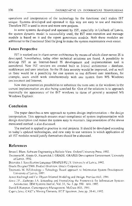
106 D A T O R Z I N A T N E U N I N F O R M A C U A S T E H N O L O G I J A S

operations and interpretation of the t echno logy by the functional shell m a k e s 1ST unique. Systems developed and opera ted in this w a y are easy to use and maintain. Therefore 1ST is used in more and more n e w projects .

In some systems developed and opera ted by 1ST, especial ly in Un ibank of Latvia, the system dynamic model is successfully used , the 1ST state-transition and message module is based on it and the report genera t ion modu le . Both these modules are additional to the Funct ional Shell he lp ing to m a k e the sys tem main tenance even easier.

Future Perspective

1ST is worked out in cl ient-server archi tec ture by m e a n s of which cl ient-server IS is developed. Never the less , today other technical so lu t ions are found. A possibil i ty to develop 1ST as an In temet-based IS deve lopmen t and implementat ion tool is considered. N e w 1ST versions are crea ted buil t in 3-level architecture - database, middleware and user interface. So the IS data securi ty would be improved, and as well as there would be a possibili ty for one sys tem to use different user interfaces, for example , users could work s imul taneous ly with one system from M S W i n d o w s envi ronment and Internet.

N e w data presentat ion possibil i t ies to subst i tute the trees seen in the w indows in the current implementa t ion are also be ing sea rched for. One of the solutions is to approach maximal ly the appearance of the 1ST w i n d o w s to those of generally accepted M S W i n d o w s Explorer.

Conclusion

The paper descr ibes a new approach to sys tem des ign implementa t ion - the design interpretation. This approach ensures exact compl i ance of sys tem implementa t ion wi th design description and makes the sys tem easy to main ta in . Implementa t ion of the above ment ioned method is also discussed.

The method is applied in pract ice in real projects . It should be developed according to today ' s updated technologies , and n e w easy to use vers ions in which applicat ion of all 1ST modules wou ld justify themse lves shou ld be elaborated.

References

Brace I. Blum. Software Engineering a Holistic View. Oxford University Press, 1992. Treimanis M.. tvrasts O., Nazartchik I. GRADE. GRAPES Development Environment. University

of Latvia, 1992. Bicevskis J. Specification Language GRAPES/PLUS. University of Latvia, 1992. Oracle Designer'2000. Product Overview. Oracle Corporation. Treimanis M. ISTchnology - Tehnology Based approach to Information System Development.

University of Latvia, 1997. James Ruabaugh and Co. Object-Oriented Modeling and Design. Prentice-Hall, 1991. Sowa J.F., Zachman J.A. Extending and Formalizing the Framework for Information Systems

Architecture. IBM Systems Journal, Vol. 3 1, No. 3. pp. 590 - 6 1 6 , 1992. David R.Hampton. Contemporary Management. McGraw-Hill, 1981. Capers Jones. CASE'S Missing Elements. IEEE Spectrum, June pp. 38-41. 1992.

L A T V I J A S U N I V E R S I T A T E S R A K S T I . 2 0 0 4 . 6 6 9 . se j . : D A T O R Z I N A T N E UN I N F O R M A C I J A S T E H N O L O G I J A S . I 0 7 . - 1 I 6 . lpp

Semantics and Equivalence of UML Class Diagrams Girts Linde

I M C S , Univers i ty of Latvia, g l inde@acm.org

One and the same "real world" can be modeled by different UML class diagrams, which in such a case can be considered "intuitively equivalent". A new approach to the formalization of this "intuitive equivalence" of class diagrams is proposed, based on the fonnal object-oriented cognitive process. Two theorems are proved to support this approach. The new formalization can be used to construct algorithms for class diagram analysis. Key words: UML, class diagrams, equivalence.

Introduction

As object model ing gains popularity, starting from the pioneering work [1], a need emerges for methods of handling and evaluating models . Object models are used in various stages of system development - from definition of requirements to system design. One problem is to validate the model as it gets transformed and refined in the lifecycle of system development . Research is already being done on this topic [2 -5] . A more general problem is to compare several alternative object models of the same "real world".

Our goal is to formalize this "intuitive equivalence" for object models represented with U M L class diagrams. Consider the class diagrams mode l ing directed graphs shown in Figure 1.

Node 1

N o d e , S ta r t s at , 1 E d g e

E n d s at

E d g e to

C o n n e c t e d to , Standpoint Standpoint

1

N o d e 1

* Endpoint

C o n n e c t e d to Endpoint

S ta r t s with

Edge

E n d s with

Fig. L Three class diagrams of a directed graph

Formally , we have here 3 totally different class diagrams. Each of them describes different instance diagrams. But intuitively we know that all three of these diagrams describe the same "real world" - directed graphs.

108 D A T O R Z I N A T N E U N I N F O R M A C U A S T E H N O L O G I J A S

In [6] a formal definition of the "intuitive equivalence" o f class diagrams is proposed called reduction. It is defined on the instance diagram level and uses composi te classes to define the transformation between the class d iagrams. In this paper a new approach to the definition of the "intuitive equivalence" of class d iagrams is proposed, called semantical implication. It is based on the formalization of the object-oriented cognitive process, introduced in [7]. T w o theorems are proved confirming that the new approach is more general and intuitive.

The paper is structured as follows. In section 2 a restricted formalization of the cognitive process is outl ined. In section 3 the new definition of the "intuitive equivalence" is presented. In section 4 the reduction of class d iagrams is briefly outlined. And finally in section 5 the difference between the two definitions of the "intuitive equivalence" is examined, proving two theorems.

The formalization of the cognitive process

The definition of the class diagram semantical implication is based on a restricted version of the formal cognit ive process (for the full version see [7]) happening in the mind of a modeler when he analyzes a fragment of the real wor ld and builds an object model for it. The fragment of the real world to be modeled , together with the object-oriented structure that gets created in the mind of the modeler we represent with a labeled directed graph and call it the cognition state (Fig. 2 ) . Dur ing the cognit ive process, as the modeler learns new concepts from the fragment of the real world, his mind is populated with new elements that correspond to objects, classes, links and associat ions. With every addition of a new element a new cognit ion state is created. The resul t ing sequence of cognition states we call the cognition path. The cognition path ends with a cognition state that contains the final object model as a part of it (Fig. 3).

State of t he abs t rac t w o r l d ,<

Sta te o f tbe-'real wDr ld

Fig. 2. A cognition state

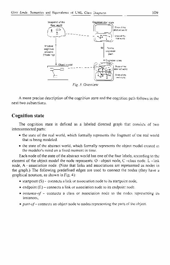
Girts Linde. S e m a n t i c s and E q u i v a l e n c e of L ' M L C l a s s D i a g r a m s 109

S n a p s h o t o f t he R e a l w o r i d

n i t i o n s tar t s t a t e

State Gf the bs l rac l w o r i d

Fig. 3. Overview

A more precise description of the cognition state and the cognition path follows in the next two subsections.

Cognition state

The cognition state is defined as a labeled directed graph that consists of two interconnected parts:

• the state of the real world, which formally represents the fragment of the real world that is being modeled.

• the state of the abstract world, which formally represents the object model created in the modeler 's mind on a fixed moment in time.

Each node of the state o f the abstract world has one of the four labels, according to the element of the object mode l the node represents: O -objec t node, C -class node, L - l ink node, A —association node. (Note that links and associations are represented as nodes in the graph.) The following predefined edges are used to connect the nodes (they have a graphical notation, as shown in Fig. 4):

• startpoint (S) - connects a link or association node to its startpoint node,

• endpoint (E) - connects a link or association node to its endpoint node.

• instance-of - connects a class or association node to the nodes representing its instances,

• part-of- connects an object node to nodes representing the parts of the object.

110 D A T O R Z I N A T N E U N I N F O R M A C U A S T E H N O L O G I J A S

Start state of the abstract world

- S -

-E-

s t a r t p o i n t

e n d p o i n t

i n s t a n c e - o f •

p a r t - o f •

Fig. 4. Notation of predefined edges

( empty )

State of the real world

s r

Fig. 5. A cognition start state

We define the cognition start state as a cognit ion state that consists of a state of the real world and an empty state of the abstract wor ld (Fig. 5).

Cognition path

During the cognitive process, a cognit ion path is incremental ly created. It is a sequence of cognition states, beginning with a cognition start state. Given a cognition state, the next cognition state is produced by extending the state of the abstract world in it - by adding a new node or by adding one of the predefined edges between the nodes. As in [6], in this paper we work with the basic class d iagrams containing classes, binary associations and the four mos t popular multiplicity constraints (0 . .1 , 1..1, 1..*, 0..*). So, the cognitive process can be restricted to use only the needed steps. W e call the resulting cognition path a constructive cognition path.

Definition. W e call a cognition path constructed us ing the following steps a constructive cognition path (CCP):

• "create a new aggregate object" (Fig. 6), which represents a subgraph of the real world state: create a node with label O, and connect it to all nodes of the subgraph by the edge part-of;

• "create a new class": create a node with label C (a class node);

• create an edge instance-of from an existing class node to any existing object node that has no instance-of edges connected to it;

• "create a new association": create a node with label A (an association node), connect it to two existing class nodes by the edge S and the edge E;

• "create a new link" (Fig. 7): create a node with label L (a link node), connect it to two existing object nodes by the edge S and the edge E;

• create an edge instance-of from an existing association node to any existing link node that has no instance-of edges connected to it; this is allowed only if the nodes connected by the link (nodes to which edges S and E go) are connected by instance-of edges to the class nodes, connected by the association (with edges S and E. respectively).

Girls Linde. S e m a n t i c s a n d E q u i v a l e n c e of U M L C l a s s D i a g r a m s 111

Fig. 6. Adding an object

r-s,„.„,... "S

(O) f

V / s£- E

F;g. 7. Adding a link

If we assign names to the class and association nodes of a given CCP then we can construct the corresponding instance diagram.

The new definition of the "intuitive equivalence"

Consider a real world state R, and two C C P s PI and P2 starting from this real world state R. If P2 can be obtained from PI aggregating some of the objects and classes while preserving some properties of the structure, then we assume that these cognition paths model the same concept in different levels of detail. A more precise definition follows.

Definition. W e say that P2 is less detailed than P I , if the following 4 conditions hold: 1) if two nodes of R in PI are connected by part-of edges to one and the same object

node (Fig. 8 a), then in P2 they are also connected by part-of edges to one and the same object node (Fig. 8 b),

Cognition path P1 Cognition path P2

(a) (b)

Fig. S. Condition for object nodes

112 D A T O R Z I N A T N E U N I N F O R M A C U A S T E H N O L O G I J A S

2) if there are two nodes a and b in R that are in P I connected by part-of edges to object nodes cl and d l , respectively, and there is a link node connected by S edge to cl and by E edge to dl (Fig. 9 a) , then in P2 they are connected by part-of edges to one object node (Fig. 9 b) or they are connected by part-of edges to object nodes c2 and d2, respectively, and there is a link node connected by S edge to c2 and by E edge to d2 (Fig. 9 c) .

C o g n i t i o n p a t h P 1 C o g n i t i o n p a t h P2

, s \ b K E

( o ) c l ( 0 ) d l

6 6 ( a )

o > 2 0 ) c 2 d2

6 b 6 6 i

(b)

Fig. 9. Condition for link nodes

(c)

3) if there are two nodes a and b in R that are in P I connected by part-of edges to object nodes cl and d l , respectively, and the object nodes cl and dl are connected by instance-of edges to the same class node (Fig. 10 a), then in P2 they are connected by part-of edges to one object node (Fig. 10 b) or they are connected by part-of edges to object nodes c2 and d2, respectively, and the object nodes c2 and d2 are connected by instance-of edges to the same class node (Fig. 10 c).

C o g n i t i o n p a t h P1 C o g n i t i o n p a t h P2

( o ) c . ( o ) d l

6 6b

( a )

O ) c 2 & (2) d2

6 b 6 6 (b)

Fie. 10. Condition for class nodes

(c)

4) if there are 4 nodes a, b . c and d in R. and PI contains 4 object nodes a l , b l , c l and d l , 2 link nodes el and f l , and an association n o d e g l , connected as in (Fig. 11 a), then in P2 there are two cases possible:

• a and b are connected by part-of edges to one and the same object node, and c and d are connected by part-of edges to one and the same object node (Fig. 11 b)

• or there is the same configuration as in P1 - there are 4 object nodes a2, b2, c2 and d2, and 2 link nodes e2 and f2, and an association node g2, connected as in Fig. 1 1 c.

Gins Linde. S e m a n t i c s a n d E q u i v a l e n c e of U M L C l a s s D i a g r a m s 113

Cognition path P1

( 0 ) a l © > > 1 (O)" ( O ) 1 1 1

Cognition path P2

C o ) * © » vo ) " 2 (") KC$ c 2 (°)'

la) lb]

f7g. / / . Condition for association nodes

N o w , using this method of comparing cognition paths we define the "intuitive equivalence" o f class diagrams, in this paper called semantical implication.

Definition. We will say that a class diagram CD1 semantically implies a class diagram CD2, if for every state of the real world R:

• if there exists a CCP PI starting from R whose corresponding instance diagram ID1 satisfies CD1,

• then there exists a CPP P2 starting from R that is less detailed than PI and whose corresponding instance diagram ID2 satisfies CD2.

Reduction of class diagrams

In [6] the "intuitive equivalence" of class diagrams is formalized as a reduction. The reduction of the more detailed diagram to the less detailed one is defined introducing a set of concepts. Every concept is represented with a composite class containing some of the existing classes and associations, and assigning multiplicity constraints to the enclosed classes. The set o f new concepts must cover all the classes o f the class diagram.

The multiplicity constraints assigned to the contained classes must guarantee that the composite classes have only connected instances. When reducing an instance diagram with a set of concepts, each group o f objects and links that forms an instance of one of the concepts is replaced with a new object, and so a new (less detailed) instance diagram is constructed.

Definition. We will say that a class diagram D l can be reduced to a class diagram D2, if there exists such a set of new concepts S, using which every instance diagram of D1 can be reduced to an instance diagram of D2 , and all instance diagrams of D2 can be constructed this way from instance diagrams o f D l .

The relation between the two definitions

In this section we show that the semantical implication is more general than the reduction.

Theorem 1. If a class diagram D l can be reduced to a class diagram D2, then Dl semantically implies D2.

114 D A T O R Z I N A T N E U N I N F O R M A C U A S T E H N O L O G I J A S

Proof.

Consider

• a class diagram Dl that can be reduced to D2 by a set of concepts S,

• a state of the real world R, for which a constructive cognition path PI exists starting from R, whose corresponding instance diagram ID1 satisfies D l ,

• an instance diagram ID2 that is reduced from ID1 using a set of concepts S.

To prove the theorem we show that w e can construct a constructive cognition path P2 starting from R that is less detailed than PI and whose corresponding instance diagram is ID2.

First we construct the last cognition state X o f P2 whose corresponding instance diagram is ID2 and which is based on the same state o f the real world R:

• group the object and link nodes and the class and association nodes into subgraphs according to the new concepts in S,

• replace each object-link subgraph with an object node, and each class-association subgraph with a class node,

• replace multiple instance-of edges between two nodes with one instance-of edge,

• replace multiple link nodes (together with S and E edges) that are between the same object nodes, and that are connected by instance-of edges to the same association node, with one link node (and one pair of S and E edges).

N o w it is easy to construct a constructive cognition path P2 that starts with the state of the real world R and ends with the state X. The cognition path P2 is constructed in the following order:

1) create aggregate object nodes with part-of edges (in any order),

2) create link nodes with S and E edges (in any order),

3) create class nodes (in any order),

4) create instance-of edges between object nodes and class nodes (in any order),

5) create association nodes with S and E edges (in any order),

6) create instance-of edges between link nodes and association nodes (in any order).

The set o f new concepts S by definition is constructed so that every class and association of D l belongs to exactly one new concept. Keeping that in mind it is easy to see that the new cognition path P2 is less detailed than the cognition path PI (all four conditions are satisfied).

Theorem 2. There exist two class diagrams D l and D 2 , such that

• D l semantically implies D2, but

• D l cannot be reduced to D2.

Proof.

Consider the two class diagrams in Fig. 12. They both describe directed graphs. The difference is that Dl al lows us to model the structure o f graphs, but for D2 every object instance is a whole graph.

Girts Linde. S e m a n t i c s a n d E q u i v a l e n c e of U M L C l a s s D i a g r a m s 115

c lass diagram D1

E d g e to c lass diagram D2

N o d e

Fig. 12. Two class diagrams of a directed graph

Let's prove that D l semantically implies D2. Consider an arbitrary state of the real world R, for which there exists a CCP PI whose corresponding instance diagram satisfies D l . We can construct a CCP P2 that starts from the same state of the real world R and contains one object node, which is connected by part-of edges to all the nodes of R, and which is connected by an instance-of edge to a class node. The corresponding instance diagram o f P2 satisfies D2 . It is easy to see that P2 is a less detailed CCP than PI.

Now, let's see if D l can be reduced to D2 . It can be proved that the only new concept that can be constructed for the diagram D l is a trivial composite class that contains the class Node, but doesn't contain the association Edge-to. The association Edge-to cannot be included in a new concept together with Node, because it forms a cycle, and cycles are not allowed inside the concept (that comes from the requirement that a new concept must have only connected instances). Therefore, D l can be reduced only to D l , but cannot be reduced to D2.

Conclusion

In the paper a new formalization approach of the U M L class diagram "intuitive equivalence" is presented. It is enabled by the semantics of class diagrams that is based on the formalization o f the object-oriented cognitive process. T w o theorems are proved to compare the two definitions of the class diagram "intuitive equivalence". The theorems confirm that the new definition is more general - the reduction is a special case of the semantical implication.

In fact, Theorem 2 can be generalized to prove that any class diagram semantically implies the trivial class diagram containing one class. That is a fundamental property of system modeling. These theoretical results show that the semantical implication is now very close to the concept o f the class diagram "intuitive equivalence". The next problem that must be researched is the algorithmical decidability of the class diagram semantical implication, as it is already done for the reduction in [6].

Finally, it must be noted that this paper gives another confirmation of the sufficient generality of the object-oriented cognitive process formalization. It is shown that the formalization can be successfully used to reason about the problems of the class diagram equivalence.

116 D A T O R Z I N A T N E U N I N F O R M A C I J A S T E H N O L O G I J A S

References

J.Rumbaugh, M.Blaha, W.Premerlani, F.Eddy W.Lorsen. Object-oriented modeling and design. Englewood Cliffs, NJ: Prentice Hall, 1991.

A.S.Evans, R.B.France, K.C.Lano, B.Rumpe. The UML as a Formal Modelling Notation. UML'98. LNCS, Vol. 1618, Springer, 1999

K.Lano, J.Bicarregui. Semantics and Transformations for UML Models. UML'98. LNCS, Vol. 1618, Springer, 1999

A.S.Evans. Reasoning with UML class diagrams. WIFT'98. IEEE CS Press, 1998 K.C.Lano, A.S.Evans. Rigorous Development in UML. FASE'99, ETAPS'99. LNCS, Vol. 1577,

Springer, 1999 G. Linde. Reduction of UML Class Diagrams. In: proceedings of the Fifth International Baltic

Conference on Databases and Information Systems. Tallinn, 2002. G. Linde. The Cartoon Method of Semantics Definition for Modeling Languages. Submitted to:

Proceedings of the Latvian Academy of Sciences. Riga, 2003.

L A T V I J A S U N I V E R S I T A T E S R A K S T I . 2 0 0 4 . 6 6 9 . se j . : D A T O R Z I N A T N E U N I N F O R M A C I J A S

T E H N O L O G I J A S . I 1 7 . - 1 2 5 . Ipp.

Requirements and Options for Data Warehouses at Universities

Laila Niedrite Lecturer at the Univers i ty of Latvia

Raina blvd. 19, Riga , Latvia , +371 7034439 lnied@lanet . lv

This paper deals with the problems of the changing role of traditional universities on the educational market, and how data warehousing could help the universities solve their problems. It describes the experience of different universities and the issues of feasibility study of the data warehousing project at the university. Key words: data warehouses, requirements, universities.

Introduction

Data w a r e h o u s i n g is tradit ionally used in bus iness . Higher education is trying to follow the g rowing trend in development and usage of data warehouses ; however , the reasons for doing it are often more concerned wi th scientific and educational issues than wi th financial benefi ts . Higher educational institutions have grown in recent years into large bus inesses and the managemen t of these insti tutions has changed and become more bus iness- l ike . The managemen t of h igher educat ional institutions can benefit from using data wa rehous ing jus t as other tradit ional bus iness organizat ions.

The topic of data warehous ing [5], [13] , [4] , and [7] comprises architectures, a lgor i thms, mode l s , tools, organizat ional and m a n a g e m e n t issues for integrating data from several operat ional sys tems in order to p rov ide information for decision support, e.g., us ing data min ing or O L A P tools. T h e data warehous ing technology provides integrated, consol ida ted and historical data. A data warehouse can be realized as a separate da tabase conta ining these integrated data.

A data warehouse is built by extract ing data from different data sources, t ransforming them and then loading into a separate database where specialized data model l ing concepts , e.g. star schema, and da tabase structures like materialized views [14] are used . Final ly, the data are accessed wi th different data analysis tools as shown in Figure 1.

118 D A T O R Z I N A T N E U N I N F O R M A C U A S T E H N O L O G I J A S

Data source systems: Students, Financing, HRM ..

The Data Warehouse target database

Data access and Analysis

f^Data Mining)

Statistics ^

Q Reporting ^

Figure J. Common data warehousing environment

This paper will give further insight into the business processes o f higher educational institutions, and some key benefits of having a data warehouse in business are examined concerning higher education.

The following section presents the business process model for higher educational institutions and university management issues in the new competit ive environment. An overview of possible areas o f application o f data warehousing in education is given in Section 2. Section 3 presents the possible system architecture for the new application area, and the relevant experience of universities using data warehousing. Section 4 draws conclusions on the data warehouse feasibility study at the University o f Latvia.

The Education Process as a Business Process

The starting point for finding out the necessity for higher education institutions to build and use data warehousing could be their traditional management and business processes. The two main university activities are education and research, and the most important support processes are human resource management and financial resource management [11] .

In the last decade universities have experienced significant changes in the education area. One of the important issues is the growing competition between educational institutions.

Colleges and universities rarely express their policies, intentions, and practices in competitive terms. However, the pressure on traditional resources doubled with the emergence of technology-based education delivery systems will force competitive thinking [6],

If w e consider education as business; w e have to define the key terms in this context. The universities as "education providers" have to find out, what is the product? What are the resources? What is the price o f the product? The students as „customers" have different important questions: from which institution to buy, which product exactly to buy? Finally, the customer will have to know about the quality and price of the product to be able to make the right decision.

Laila Niedrite. R e q u i r e m e n t s a n d O p t i o n s for D a t a W a r e h o u s e s at U n i v e r s i t i e s 119

There are many examples of using the market terminology in higher education now. One of the best known cases in this area is the University of Phoenix, which focuses on educational needs o f adults. The new trend is the formation and growth of corporate educational institutions, many of which have become universities with accredited study programs in recent years. For example, Motorola University co-operates with universities around the world to develop and deliver courses for the Motorola Corporation employees.

The most challenging issues for university management in the new competitive environment are [12]:

• Public relations,

• Competition, including universities abroad,

• Market analysis,

• Strategic planning,

• Revenues/ expend iture analysis,

• Calculation of expenses,

• Cooperation with traditional businesses.

Alongside developing their policies in the new competitive environment, universities are looking for methods to help them evaluate the answers and to support them and their customers to make the right decisions.

Higher education is facing many problems in the next years and IT will play a major role in determining how institutions resolve and solve these problems [15] . Many universities are looking at data warehousing with the hope that it can help them to solve their problems.

The reasons w h y data warehouses are developed and successfully used in management and decision support in traditional business areas like sales, banking and others are the following:

• the data warehouse makes the information in the organization more accessible,

• integrates data from many operational data sources and thus ensures quick access to the information about business activities of the whole organization

• the data are user-friendly and consistent.

As it has been mentioned above, the universities' main activities are education, research and management, and also the new business activities, for example, processes which become important for the existence and development of universities. Therefore, we can assume that universities, like businesses, can benefit from data warehousing.

The following section deals with some scenario examples for data warehouse development at universities, which are connected with the traditional higher education institution's processes (scenarios 3 and 4) and also with the new business processes (scenarios 1 and 2).

120 DATORZINATNE UN INFORMACUAS TEHNOLOGIJAS

Specifications for the University Data Warehouse

There are some attractive university data warehouse implementation scenarios. Components of them have been implemented at European and American universities [1] , [2], [3] .

Data warehouse implementation scenario 1.

The first specification is about attracting good students. With the ever escalating costs and competition associated with higher education, universities and col leges are very interested in attracting and retaining high-quality students [8].

A data warehouse can enhance the existing information system that handles admissions to university study programmes, providing access To the required information. One example data warehouse star schema for the admission process is shown in Figure 3. The star schema reflects the current administrative processes for student admission in the IS o f the University o f Latvia.

rime

PK T i m e kev

D a t e Month Y e a r A c a d e m i c year

Faculty

PK Facultv kev PK

Facul ty_code N u m b e r student

Admisian fact

PK Time admiss FK PK Time e x a m l FK PK Time exam2 FK PK Time results FK PK Proaramme FK PK ADDlicant FK PK Faculty FK

Sta tus > -

G r a d e l Grade2 Priority

Study Programme

PK Proaramme kev

D e g r e e No_of_appl tcants N o _ o f _ a p p r o v e d M a x _ g r a d e _ a p p r o v e d Start ef fect ive da ta

Applicant

PK ADDlicant kev

First n a m e Family n a m e Date of birth S t u d e n t n u m b e r S e x A d d r e s s

Figure 3. Example data warehouse star schema for admissions.

For example [1] , if the admission algorithm is based on school grades and selected number o f study programmes in priority order, the information about the admission process in previous years could help applicants avoid mistakes in choosing the programmes, because they do not really comprehend the selection algorithm.

Data warehouse implementation scenario 2

The next specification is to support customer relationship management (CRM) strategies.

Luila Niedrite. Requirements and Options for Data Warehouses at Universities 121

'CRM aligns business processes with customer strategies to build customer loyalty and increase profits over time.' (Harvard Business Review, 2002) .

Each year colleges and universities confront the challenge of meeting higher levels of service demanded by an increasingly sophisticated and competitive marketplace and consumer base. At the same time there is an ever present need to cut costs and tighten budgets. Therefore, it becomes more and more important for each service interaction to be effective in both cost and outcome. In order to do this, a greater understanding o f the customer is critical [9] .

Universities are now challenged with the needs of many different groups of learners. The universities are working with multi-generational students, and also the correspondence students are expecting new services. Another important issue is the feature o f learners in the information age to get information when and how they choose.

Universities must now evaluate their services taking into account that the students are customers. Universities are starting to develop new strategies to manage their customer relationships in various stages o f the student's lifecycle. The universities have to think about new services in each phase o f the lifecycle to support students' different needs on the way towards graduation.

There are some additional outcomes with effective CRM strategy: reduced costs, if the self-service is supported with web—applications; improved document flow in the institution and influence on new technologies and investments.

Data warehouse implementation scenario 3

This scenario focuses on the improvement o f the study process [2], for example, the assessment o f study courses concerning the student and course performance. The evaluation o f detailed statistics such as the number of students enrolled, evaluated and approved, the average mark, and the average approved mark can help to find out the potential problems for a particular course before they arise. It helps better understand the student needs, or in business terms, what are the students buying?

Another issue is the quality assessment o f the study programme. Statistics on admissions, new students, drop-outs and graduates and average studying duration before graduation can give the faculty management the necessary feedback and can influence how the programme works and changes.

Another possible way to conduct course and study programme evaluation is by getting information from student questionnaires and by publication of aggregated data for all participants: students, lecturers and managers.

Data warehouse implementation scenario 4

This scenario describes resource planning at the university, for example, planning the teaching service. If the managers o f the faculty plan the necessary number o f classes for a particular course, they must know the statistics about the previous year. It can help to avoid empty or full classes and to find out the workload of teaching staff.

Another example is Human Resources, when saving all transactions made with university personnel records can help plan the carrier of employees and make the right decisions about new recruitments.

122 D A T O R Z I N A T N E U N I N F O R M A C U A S T E H N O L O G I J A S

The financial resources of a university, in context with the size of the student body, as scientific results over several years are also very significant issues to analyze.

One less obvious example [3] for this scenario aims to measure the international attractiveness o f the institution. The purpose is to control the institution's policy on its international reputation and exchanges, with budget involved.

Data Warehouse and University Information Technology Architecture

Because many universities' data warehousing scenarios mentioned above are concerned with Customer Relationship Management (CRM), it is necessary to understand the role o f the data warehouse in the university IT architecture and its connection with CRM applications

The Connect Enterprise Architecture [9] also fits for universities and illustrates as in Figure 4, how CRM integrates many existing applications into a unified customer facing strategy.

Students Employees Management Alumni

Application Intsgratinn Customer relationship management

Infnrmatinn C^Data m i n ^ n g ^ ) < ^ ^ e p o m r v g ^ > < ^ ^ 0 1 ^ p ~ analysis

Data Integration Data warehouse

IS-data source

Figure 4. Data warehouse connections with CRM applications.

The layer of Enterprise Application Integration provides access to Back Office applications (ERP, Student IS . . . ) from various solutions: data mining, CRM applications, Portals, Knowledge Management applications.

The integration o f Back Office Applications' data can be solved by using a data warehouse. The data warehouse also serves the reporting and analytical needs of an

Laikt Niedrite. R e q u i r e m e n t s a n d O p t i o n s for D a t a W a r e h o u s e s at Un ive r s i t i e s 123

institution, so the data warehouse can be a part of CRM solution which focuses on front office activities, e.g., customer service and support.

The present developments in universities in the field of data warehousing are very different in their decisions, which architecture and tools to use, and also which business processes to support with data warehousing solutions.

A m o n g higher education institutions in the USA, less than 25% have or are planning a data warehouse [10] . Only a limited number of database tools is used.

The choice mostly depends on existing environments in other projects at the university. This is also true for client tools. The most popular is the ORACLE database and Web based client side tools.

Only a very small number of universities have all their information sources integrated into a corporate warehouse. Most are starting with students' data, human resources or finance data.

Many data warehousing projects in universities have been initiated in the IT department, and not all o f them have obtained management sponsorship yet.

N o similar survey has been done in Europe, and to asses the situation with data warehouses in European universities one has to look up the information on the Internet and the annual conference 'European Universities Information Systems' (EUNIS). The number of participating universities from different countries is usually around 100 every year, but during the last 5 years, the number o f presentations on data warehouses was less than 10. For example, in 1999 there were 2 presentations from Ljubljana in Slovenia and from Porto in Portugal. The most significant data warehouse project in Europe among universities is in France, where the project is developed on a national scale. All French universities which had previously implemented the university information system A P O G E E (also a national-scale project) can now participate in the data warehouse project.

The Data Warehouse Feasibility Study at The University of Latvia

As an example of a university starting the development of the university data warehouse w e can consider the University o f Latvia. The following issues are important at the starting point of the project:

The existence and quality of data sources

In the case o f the University of Latvia, an information system was developed based on the Oracle database and Oracle Application Server. During the 5 years of the system development and implementation process, a large amount of various data have been collected. It is now possible to provide access to operational data, but the possibility to analyze historical data in different ways is limited. One of the questions for the evaluation o f the feasibility of the data warehouse is the technical feasibility, which means the existence o f data for expected data warehouse and the quality of existing data. At the University o f Latvia the management information system (LUIS in Latvian) has been developed since 1996. The starting year of the students' module was 1997, of the study fees module - 1998, of the courses and courses' enrolment module - 2000, and the starting year of the admission module was 1998. The data accuracy differs not

124 D A T O R Z I N A T N E U N I N F O R M A C U A S T E H N O L O G I J A S

depending on the module, but on the faculty, in some cases it depends on a particular program of study. The existing data are accurate enough, but in some cases the lack of data is obvious. The second possible data source for the data warehouse at the University of Latvia in addition to LUIS is the accounting system.

Reasons for having a data warehouse

For example, one reason for starting a feasibility study o f a data warehousing project at the University of Latvia is burdened access to the necessary information in the operational systems. Another reason is the growth o f competition among universities and the new roles of traditional universities. One more question regarding readiness is the business motivation of the institution. The business motivation of the University of Latvia is based on the changing situation in education, which was described earlier in this paper. The management o f the University o f Latvia is interested in a more flexible reporting facility, in the analysis of the integrated information, and the most actual need is a new portal. The idea o f the portal fits CRM solutions and also fits the data warehouse as a data integrator.

Users' acceptance

Prior to starting a data warehouse project it is important to understand the readiness of the institution to have a data warehouse [7] . One of the questions for evaluation is the existence o f data for the expected data warehouse. A l so an important question is the readiness of people to use the data warehouse information. In the University o f Latvia the users have long experience in usage o f operational systems, and if the data warehouse will satisfy also the reporting needs of the users, the acceptance of the data warehouse will depend on the correctness of extracted data and reports. The users were also involved in the requirements analysis.

The decision between different development scenarios and the right choice for the first development stage.

The possible scenarios regarding specifications have to be presented to the university management and discussed. The information about users' needs and priorities help to make the right decision. In our case study w e collected information about the number of potential users and about the purposes o f the usage. W e evaluated this information to get quantitative measurements expressing the more urgent needs. The earlier mentioned 4 * implementation scenario's subset of problems concerning the human resources and the financial resources of the university in context with the number of students, and scientific results were accepted as the starting point of the implementation.

Conclusions

Universities are not the typical owners of a data warehouse system, because the data warehouse projects need financial investments, which in the case of universities, are not obviously comparable with gained results in terms of money. The reasons why universities have or are starting the development of the data warehouse are only in the long term the expected return on investment, or the growing competition. According to

Laila Niedrite. R e q u i r e m e n t s and O p t i o n s for D a t a W a r e h o u s e s at U n i v e r s i t i e s 125

their prior business functions and goals, universities build data warehouses to improve the quality o f education and communication with their customers - students. The improvement of the existing reporting facility o f operational systems and improvement of data accessibility can be mentioned as a secondary reason.

References

[I] Bajec,M., Rupnik.R., Krisper,M. Using Data Warehouses in University Information Systems, Proceedings of conference EUNIS99, Espoo, Finland, 1999.

[2] David,G., Ribeiro.L. Getting Management Support from a University Information System. Proceedings of conference EUNIS99, Espoo, Finland, 1999.

[3] DesnosJ.F. A National Data Warehouse Project for French Universities, Proceedings of conference EUNIS2001, Berlin, 2001.

[4] Hammer.J., Garcia-Molina,H., Widom,J., Labio.W., Zhuge,Y. The Stanford Data Warehousing Project.

[5] Inmon,W.H. Building the Data Warehouse, John Wiley, 1996. [6] Katz,R.N. Competitive Strategies for Higher.Education in the Information Age, Proceedings

of conference EUNIS99, Espoo, Finland, 1999. [7] Kimball,R., Reeves,L., Ross,M., Thornthwite,W. The Data Warehouse Lifecycle Toolkit,

John Wiley, 1998. [8] KimbalfR., Ross M. The Data Warehouse Toolkit: The Complete Guide to Dimensional

Modeling, John Wiley, 2002. [9] KPMG Consulting, Managing Customer Relationships in Higher Education, 2002 [10] NCHEMS, Information Architecture: the Data Warehouse Foundation, CAUSE/EFFECT ,

Volume 20, Number 2, Summer 1997, pp. 31-33, 38-40, 60. [II] Sinz, E. J.; Bohnlein, M.; Ulbrich-vom Ende, A.: Konzeption eines Data Warehouse-

Systems fur Hochschulen. In: Workshop "Unternehmen Hochschule" (Inforniatik'99, 29. Jahrestagung der Gesellschaft fur Informatik, Paderbom, 5.-9. Oktober), 1999, S. 111-124.

[12] Stonis J., Augstaka izglitlba ka pakalpojumu tirgus dallbnieks, LU konference, 2003. [13] WidomJ. (ed). Special Issue on Materialized Views and Data Warehousing, IEEE Data

Engineering Bulletin, June 1995. [14] YangJ. , Karlapalem,K., Li,Q. Algorithms for Materialized View Design in Data

Warehousing Environment, Proceedings of the 2 3 r d International Conference on Very Large Data Bases, Athens, Greece, August 1997.

[15] Zastrocky, M.R. The Information- and Technology- Enabled University of 2004, Proceedings of conference EUNIS99, Espoo, Finland, 1999.