28 September 2004

Virtual Prototyping and Performance Analysis of RapidIO-based System Architectures for Space-Based Radar

David Bueno, Adam Leko, Chris Conger,

Ian Troxel, and Alan D. George

HCS Research Laboratory

College of Engineering

University of Florida

28 September 2004 2

Outline

I. Project OverviewII. Background

I. RapidIO (RIO)II. Ground-Moving Target Indicator (GMTI)

III. Partitioning MethodsIV. Modeling Environment and Models

I. Compute node and RIO endpoint modelsII. RapidIO switch modelIII. GMTI modelsIV. System and backplane model

V. Experiments and ResultsI. Result latencyII. Switch memory utilizationIII. Parallel efficiency

VI. Conclusions

28 September 2004 3

Project Overview

Simulative analysis of Space-Based Radar (SBR) systems using RapidIO interconnection networks RapidIO (RIO) is a high-performance, switched interconnect for

embedded systems Can scale to many nodes Provides better bisection bandwidth than existing bus-based technologies

Study optimal method of constructing scalable RIO-based systems for Ground Moving Target Indicator (GMTI) Identify system-level tradeoffs in system designs Discrete-event simulation of RapidIO network,

processing elements, and GMTI algorithm Identify limitations of RIO design for SBR Determine effectiveness of various GMTI algorithm

partitionings over RIO network

Image courtesy [1]

28 September 2004 4

Background- RapidIO

Three-layered, embedded system interconnect architecture Logical – memory mapped I/O, message passing, and globally shared memory Transport Physical – serial and parallel

Point-to-point, packet-switched interconnect Peak single-link throughput ranging from 2 to 64 Gb/s Focus on 16-bit parallel LVDS RIO implementation for satellite systems

Image courtesy [2]

28 September 2004 5

Background- GMTI

GMTI used to track moving targets on ground Estimated processing requirements range from

40 (aircraft) to 280 (satellite) GFLOPs GMTI broken into four stages:

Pulse Compression (PC) Doppler Processing (DP) Space-Time Adaptive Processing (STAP) Constant False-Alarm Rate detection (CFAR)

Incoming data organized as 3-D matrix (data cube) Data reorganization (“corner turn”) necessary between stages for processing efficiency Size of each cube dictated by Coherent Processing Interval (CPI)

PulseCompression

DopplerProcessing

Space-TimeAdaptive

Processing(STAP)

ConstantFalse Alarm

Rate(CFAR)

Receive Cube

Send Results

Corner Turn Partitioned along range dimension

Partitioned along pulse dimension

DATA CUBE

Ranges

Puls

es

28 September 2004 6

GMTI Partitioning Methods- Straightforward

Data cubes divided among all Processing Elements (PEs) Partitioned along optimal dimension for any particular stage Data reorganization between stages implies personalized all-to-all

communication (corner turn) stresses backplane links Minimal latency

Entire cube must be processed within one CPI to receive next cube

Incoming Data Cube

to PE 1

to PE 2

...toPEn

time

1 CPI

PE#4

PE#3

PE#2

PE#1

PE#4

PE#3

PE#2

PE#1

PE#4

PE#3

PE#2

PE#1

PE#4

PE#3

PE#2

PE#1

PC DP STAP CFAR

28 September 2004 7

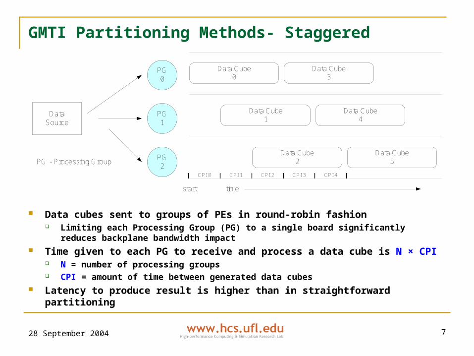
GMTI Partitioning Methods- Staggered

Data cubes sent to groups of PEs in round-robin fashion Limiting each Processing Group (PG) to a single board significantly reduces

backplane bandwidth impact Time given to each PG to receive and process a data cube is N × CPI

N = number of processing groups CPI = amount of time between generated data cubes

Latency to produce result is higher than in straightforward partitioning

DataSource

PG0

PG1

PG2

PG - Processing Group

Data Cube0

Data Cube1

Data Cube2

Data Cube3

Data Cube4

Data Cube5

timestart

CPI 0 CPI 1 CPI 2 CPI 3 CPI 4

28 September 2004 8

GMTI Partitioning Methods- Pipelined

Each PE group assigned to process a single stage of GMTI Groups may have varying numbers of PEs depending upon processing

requirements of each stage Potential for high cross-system bandwidth requirements

Irregular and less predictable traffic distribution Frequent communication between different group sizes

Latency to produce result is higher than straightforward method One result emerges each CPI, but the results are three CPIs old

PE #7

PE #5

PE #4

PE #3

PE #2

PE #1

PE #9

PE #6

PE #8

PulseCompression

Doppler Processing STAP + CFAR

28 September 2004 9

Model Library Overview

Modeling library created using Mission Level Designer (MLD), a commercial discrete-event simulation modeling tool C++-based, block-level, hierarchical modeling tool

Algorithm modeling accomplished via script-based processing All processing nodes read from a global script file to determine when/where

to send data, and when/how long to compute Our model library includes:

RIO central-memory switch Compute node with RIO endpoint GMTI traffic source/sink RIO logical message-passing layer Transport and parallel physical

layers

Model of Compute Nodewith RIO Endpoint

28 September 2004 10

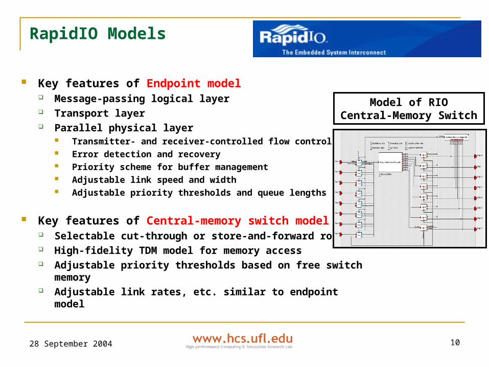
RapidIO Models

Key features of Endpoint model Message-passing logical layer Transport layer Parallel physical layer

Transmitter- and receiver-controlled flow control Error detection and recovery Priority scheme for buffer management Adjustable link speed and width Adjustable priority thresholds and queue lengths

Key features of Central-memory switch model Selectable cut-through or store-and-forward routing High-fidelity TDM model for memory access Adjustable priority thresholds based on free switch memory Adjustable link rates, etc. similar to endpoint model

Model of RIOCentral-Memory Switch

28 September 2004 11

GMTI Processor Board Models

System contains many processor boards connected via backplane Each processor board contains one RIO switch and four

processors Processors modeled with three-stage

finite state machine Send data Receive data Compute

Behavior of processors controlledwith script files Script generator converts high-level

GMTI parameters to script Script is fed into simulations

Model ofFour-Processor Board

Scriptgenerator

SimulationGMTI & system parameters

Processor scriptsend…

receive…

28 September 2004 12

System Design Constraints

16-bit parallel 250MHz DDR RapidIO links (1 GB/s) Expected radiation-hardened component performance by time RIO and

SBR ready to fly in ~2008 to 2010 Systems composed of processor boards interconnected by RIO

backplane 4 processors per board 8 Floating-Point Units (FPUs) per processor One 8-port central-memory switch per board; implies 4 connections to

backplane per board Baseline GMTI algorithm parameters:

Data cube: 64k ranges, 256 pulses, 6 beams CPI = 256ms Requires ~3 GB/s of aggregate throughput from source to sink to meet

real-time constraints

28 September 2004 13

7-Board System

Backplane and System Models

High throughput requirements for data source and corner turns require non-blocking connectivity between all nodes and data sources

4-Switch Non-blocking Backplane

Backplane-to-Board 0, 1, 2, 3 Connections

Backplane-to-Board 4, 5, 6, and Data Source Connections

28 September 2004 14

Overview of Experiments

Experiments conducted to evaluate strengths and weaknesses of each partitioning method

Same switch backplane used for each experiment Varied data cube size

256 pulses, 6 beams for all tests Varied number of ranges from 32k to 64k

Several system sizes used Analysis determined that 7-board configuration necessary for

straightforward method to meet deadline Both 6- and 7-board configurations used for pipelined method Staggered method does not benefit from a system larger than 5 boards

with configuration used Staggering performed with one processor board per group Larger system-configurations leave processors idle

28 September 2004 15

Result Latency Comparison

Result latency is interval from data arrival until results reported

Straightforward achieved lowest latency, required most processor boards No result for 64k ranges because

system could not meet real-time deadline

Staggered requires least number of processor boards to meet deadline Efficient system configuration,

small communication groups Tradeoff is result latency

Pipelined method a compromise

0

256

512

768

1024

1280

1536

32000 40000 48000 56000 64000

Number of ranges

Lat

ency

(m

s)

Straightforward, 7 boards

Staggered, 5 boards

Pipelined, 6 boards

Pipelined, 7 boards

28 September 2004 16

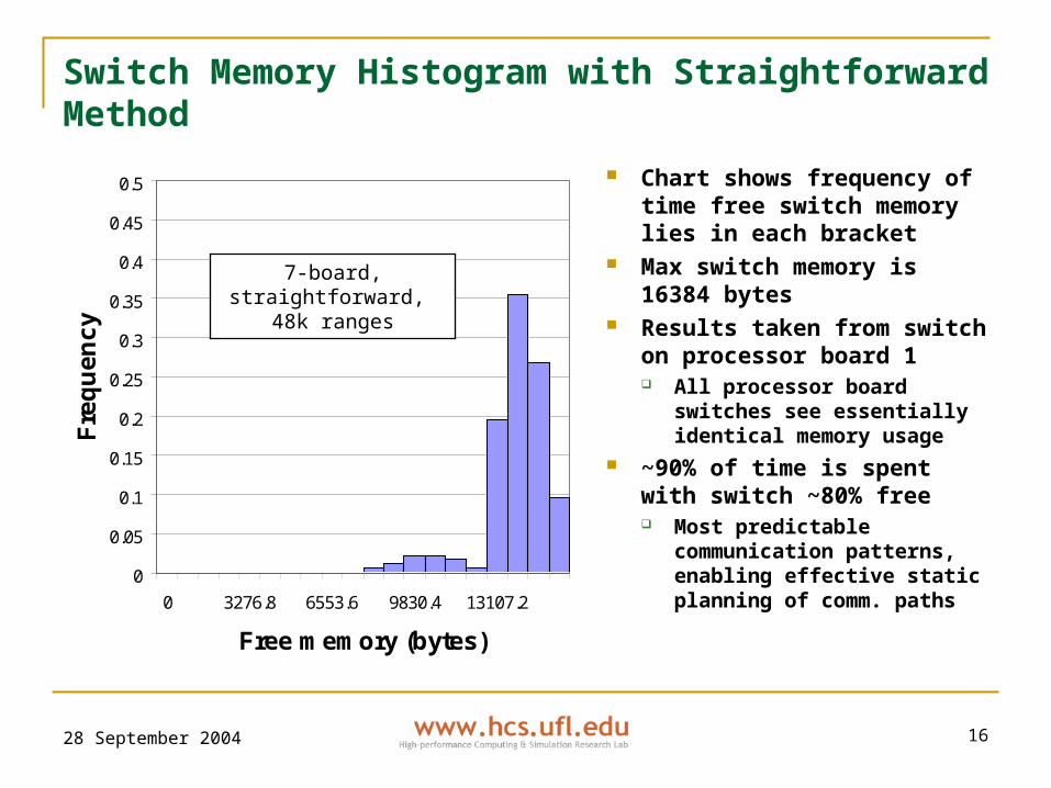
Switch Memory Histogram with Straightforward Method

0

0.05

0.1

0.15

0.2

0.25

0.3

0.35

0.4

0.45

0.5

0 3276.8 6553.6 9830.4 13107.2

Free memory (bytes)

Fre

qu

en

cy

Chart shows frequency of time free switch memory lies in each bracket

Max switch memory is 16384 bytes

Results taken from switch on processor board 1 All processor board

switches see essentially identical memory usage

~90% of time is spent with switch ~80% free Most predictable

communication patterns, enabling effective static planning of comm. paths

7-board, straightforward, 48k ranges

28 September 2004 17

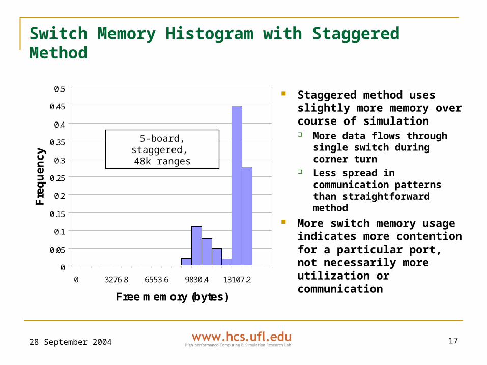
Switch Memory Histogram with Staggered Method

0

0.05

0.1

0.15

0.2

0.25

0.3

0.35

0.4

0.45

0.5

0 3276.8 6553.6 9830.4 13107.2

Free memory (bytes)

Fre

qu

en

cy

Staggered method uses slightly more memory over course of simulation More data flows through

single switch during corner turn

Less spread in communication patterns than straightforward method

More switch memory usage indicates more contention for a particular port, not necessarily more utilization or communication

5-board, staggered, 48k ranges

28 September 2004 18

Switch Memory Histogram with Pipelined Method

0

0.05

0.1

0.15

0.2

0.25

0.3

0.35

0.4

0.45

0.5

0 3276.8 6553.6 9830.4 13107.2

Free memory (bytes)

Fre

qu

en

cy

Pipelined method stresses network Irregular comm. patterns Greater possibility for

output port contention Non-blocking network not

helpful when multiple senders vying for same destination

Difficult to plan out optimal comm. paths beforehand Much synchronization

required to stagger many-to-one communication, but not extremely costly in total execution time

7-board, pipelined, 48k ranges

28 September 2004 19

Average Parallel Efficiency

Parallel efficiency defined as sequential execution time (i.e. result latency) divided by N times the parallel execution time N = number of processors that work on a single CPI Pipelined efficiency a special case, must use N/3 for fair comparison (shown) since all processors do not work on a CPI at the same

time Staggered method most efficient due to small communication groups and low number of processors working on same

CPI Straightforward method worst for opposite reason, pipelined method a compromise

0

0.1

0.2

0.3

0.4

0.5

0.6

0.7

0.8

Straightforward,7 boards

Staggered,5 boards

Pipelined,6 boards

Pipelined,7 boards

Eff

icie

ncy

28 September 2004 20

Conclusions

Developed suite of simulation models and mechanisms for evaluation of RapidIO designs for space-based radar

Evaluated three partitioning methods for GMTI over a fixed RapidIO non-blocking network topology

Straightforward partitioning method produced lowest result latencies, but least scalable Unable to meet real-time deadline with our maximum data cube size

Staggered partitioning method produced worst result latencies, but highest parallel efficiency Also able to perform algorithm with least number of processing boards Important for systems where power consumption, weight are a concern

Pipelined partitioning method is a compromise in terms of latency, efficiency, and scalability, but heavily taxes network

RapidIO provides feasible path to flight for space-based radar Future work to focus on additional SBR variants (e.g. Synthetic Aperture

Radar) and experimental RIO analysis

28 September 2004 21

Bibliography

[1] http://www.afa.org/magazine/aug2002/0802radar.asp[2] G. Shippen, “RapidIO Technical Deep Dive 1: Architecture & Protocol,” Motorola Smart

Network Developers Forum, 2003.[3] “RapidIO Interconnect Specification (Parts I-IV), ” RapidIO Trade Association, June

2002.[4] “RapidIO Interconnect Specification, Part VI: Physical Layer 1x/4x LP-Serial

Specification,” RapidIO Trade Association, June 2002.[5] M. Linderman and R. Linderman, “Real-Time STAP Demonstration on an Embedded

High Performance Computer,” Proc. of the IEEE National Radar Conference, Syracuse, NY, May 13-15, 1997.

[6] “Space-Time Adaptive Processing for Airborne Radar,” Tech. Rep. 1015, MIT Lincoln Laboratory, 1994.

[7] G. Schorcht, I. Troxel, K. Farhangian, P. Unger, D. Zinn, C. Mick, A. George, and H. Salzwedel, “System-Level Simulation Modeling with MLDesigner,” Proc. of 11th IEEE/ACM International Symposium on Modeling, Analysis, and Simulation of Computer and Telecommunications Systems (MASCOTS), Orlando, FL, October 12-15, 2003.

[7] R. Brown and R. Linderman, “Algorithm Development for an Airborne Real-Time STAP Demonsttration,” Proc. of the IEEE National Radar Conference, Syracuse, NY, May 13-15, 1997.

[8] A. Choudhary, W. Liao, D. Weiner, P. Varshney, R. Linderman, M. Linderman, and R. Brown, “Design, Implementation and Evaluation of Parallel Pipelined STAP on Parallel Computers,” IEEE Trans. on Aerospace and Electrical Systems, vol. 36, pp 528-548, April 2000.

28 September 2004 22

Acknowledgements

We wish to thank Honeywell Space Systems in Clearwater, FL for their funding and technical guidance in support of this research.

We wish to thank MLDesign Technologies in Palo Alto, CA for providing us the MLD simulation tool that made this work possible.