david m. rosen
TRANSCRIPT

Certifiably Correct SLAM
by
David M. Rosen
B.S., California Institute of Technology (2008)M.A., The University of Texas at Austin (2010)
Submitted to the Department of Electrical Engineering and ComputerScience
in partial fulfillment of the requirements for the degree of
Doctor of Science
at the
MASSACHUSETTS INSTITUTE OF TECHNOLOGY
September 2016
c David M. Rosen, MMXVI. All rights reserved.
The author hereby grants to MIT permission to reproduce and todistribute publicly paper and electronic copies of this thesis documentin whole or in part in any medium now known or hereafter created.
Author . . . . . . . . . . . . . . . . . . . . . . . . . . . . . . . . . . . . . . . . . . . . . . . . . . . . . . . . . . . . . . . .Department of Electrical Engineering and Computer Science
August 31, 2016
Certified by. . . . . . . . . . . . . . . . . . . . . . . . . . . . . . . . . . . . . . . . . . . . . . . . . . . . . . . . . . . .Professor John J. Leonard
Samuel C. Collins Professor of Mechanical and Ocean EngineeringThesis Supervisor
Accepted by . . . . . . . . . . . . . . . . . . . . . . . . . . . . . . . . . . . . . . . . . . . . . . . . . . . . . . . . . . .Professor Leslie A. Kolodziejski
Chair, EECS Committee on Graduate Students

2

Certifiably Correct SLAM
by
David M. Rosen
Submitted to the Department of Electrical Engineering and Computer Scienceon August 31, 2016, in partial fulfillment of the
requirements for the degree ofDoctor of Science
Abstract
The ability to construct an accurate model of the environment is an essential capabil-ity for mobile autonomous systems, enabling such fundamental functions as planning,navigation, and manipulation. However, the general form of this problem, simul-taneous localization and mapping (SLAM), is typically formulated as a maximum-likelihood estimation (MLE) that requires solving a nonconvex nonlinear program,which is computationally hard. Current state-of-the-art SLAM algorithms addressthis difficulty by applying fast local optimization methods to compute a critical pointof the MLE. While this approach has enabled significant advances in SLAM as apractical technology by admitting the development of fast and scalable estimationmethods, it provides no guarantees on the quality of the recovered estimates. Thislack of reliability in existing SLAM algorithms in turn presents a serious barrier tothe development of robust autonomous systems generally.
To address this problem, in this thesis we develop a suite of algorithms for SLAMthat preserve the computational efficiency of existing state-of-the-art methods whileadditionally providing explicit performance guarantees. Our contribution is threefold.
First, we develop a provably reliable method for performing fast local optimizationin the online setting. Our algorithm, Robust Incremental least-Squares Estimation(RISE), maintains the superlinear convergence rate of existing state-of-the-art onlineSLAM solvers while providing superior robustness to nonlinearity and numerical ill-conditioning; in particular, we prove that RISE is globally convergent under verymild hypotheses (namely, that the objective is twice-continuously differentiable withbounded sublevel sets). We show experimentally that RISE’s enhanced convergenceproperties lead to dramatically improved performance versus alternative methods onSLAM problems exhibiting strong nonlinearities, such as those encountered in visualmapping or when employing robust cost functions.
Next, we address the lack of a priori performance guarantees when applying localoptimization methods to the nonconvex SLAM MLE by proposing a post hoc verifica-tion method for computationally certifying the correctness of a recovered estimate forpose-graph SLAM. The crux of our approach is the development of a (convex) semidef-inite relaxation of the SLAM MLE that is frequently exact in the low to moderate
3

measurement noise regime. We show that when exactness holds, it is straightforwardto construct an optimal solution 𝑍* for this relaxation from an optimal solution 𝑥* ofthe SLAM problem; the dual solution 𝑍* (whose optimality can be verified directlypost hoc) then serves as a certificate of optimality for the solution 𝑥* from whichit was constructed. Extensive evaluation on a variety of simulated and real-worldpose-graph SLAM datasets shows that this verification method succeeds in certifyingoptimal solutions across a broad spectrum of operating conditions, including thosetypically encountered in application.
Our final contribution is the development of SE-Sync, a pose-graph SLAM in-ference algorithm that employs a fast purpose-built optimization method to directlysolve the aforementioned semidefinite relaxation, and thereby recover a certifiablyglobally optimal solution of the SLAM MLE whenever exactness holds. As in the caseof our verification technique, extensive empirical evaluation on a variety of simulatedand real-world datasets shows that SE-Sync is capable of recovering globally optimalpose-graph SLAM solutions across a broad spectrum of operating conditions (includ-ing those typically encountered in application), and does so at a computational costthat scales comparably with that of fast Newton-based local search techniques.
Collectively, these algorithms provide fast and robust inference and verificationmethods for pose-graph SLAM in both the online and offline settings, and can bestraightforwardly incorporated into existing concurrent filtering smoothing architec-tures. The result is a framework for real-time mapping and navigation that preservesthe computational speed of current state-of-the-art techniques while delivering certi-fiably correct solutions.
Thesis Supervisor: Professor John J. LeonardTitle: Samuel C. Collins Professor of Mechanical and Ocean Engineering
4

Acknowledgments
While there may only be one author listed on the title page of this document, the
production of a doctoral thesis, like most scientific endeavors, is a team effort, and I
am deeply grateful to the many friends and colleagues who have contributed to the
success of this enterprise.
First and foremost, I would like to thank my doctoral advisor John Leonard for
enabling me to come to MIT, and for his unwavering and enthusiastic support of my
research program, especially for those projects in which the approach was unortho-
dox and the outcome far from certain at the outset. Having the freedom to pursue
investigations wherever they lead at an institution as intellectually vibrant as MIT
has been a truly superlative experience.
I have also been privileged to collaborate with an extraordinarily talented and
generous group of postdoctoral scholars and research scientists over the course of my
graduate studies. I am particularly indebted to Michael Kaess, whose work on online
mapping methods inspired me to seek out the Marine Robotics Group at CSAIL, and
who very graciously supported my rooting around in the codebase for his signature
algorithms as part of my first real research project as a graduate student.1 I have
likewise been extraordinarily fortunate to collaborate with Luca Carlone and Afonso
Bandeira on the development of the semidefinite relaxation methods for pose-graph
SLAM that form the second half of this thesis; if I could have drafted my own fantasy
team of researchers for this project, I would have picked them, and working alongside
them on it has been an absolute joy.
I would also like to thank the other members and affiliates of the Marine Robotics
Group for being such wonderful colleagues. Special thanks to Maurice Fallon, Liam
Paull, Andrea Censi, Michael Novitzky, Mark van Middlesworth, Ross Finman, De-
hann Fourie, Sudeep Pillai, Janille Maragh, Julian Straub, Pedro Teixeira, and Mei
Cheung for putting up with me for as long as they have. Their good humor and
willingness to engage in regular “vigorous intellectual exercise” have made going to
1This ultimately led to the development of the RISE algorithm reported in this thesis.
5

work (and particularly conferences) both edifying and tremendously fun.
Aside from work, I am beyond grateful for the many friends both here in Cam-
bridge and around the world that have made this six-year period the wonderful ex-
perience that it has been; this has truly been an embarrassment of riches far beyond
what could properly be accounted here. Special thanks to the extended Sidney-Pacific
Graduate Community (particularly Ahmed Helal, Burcu Erkmen, Jit Hin Tan, Matt
and Amanda Edwards, George Chen, Boris Braverman, Dina El-Zanfaly, Rachael
Harding, Fabián Kozynski, Jenny Wang, Brian Spatocco, and Tarun Jain) for mak-
ing MIT feel like home, to the extended Lloyd House alumni (particularly Kevin Watts
and Melinda Jenkins, Tim and Chelsea Curran, Joe Donovan, Vamsi Chavakula and
Christina Weng, Vivek and Karthik Narsimhan, Matt Lew, Hanwen Yan, Chi Wan
Ko, and Stephen Cheng) for friendship that has spanned decades(!) and continents,
and to Christina Zimmermann for her patience, support, and good humor during the
final hectic sprint to complete my defense and this document.
And finally, tremendous thanks to my family for their enduring patience and
support throughout my time at MIT. Special thanks to my mom, who has been the
recipient of more than her fair share of odd-hours dark-night-of-the-soul phone calls
during the more difficult periods of this research (years 4–5),2 and to my grandfather
Arthur Adam, for showing me the pleasure of finding things out. Without them, none
of this would have been possible.
2Confidential to future graduate students: this will happen to you too. Brace yourselves!
6

Contents
1 Introduction 17
1.1 Motivation . . . . . . . . . . . . . . . . . . . . . . . . . . . . . . . . . 17
1.2 Contributions . . . . . . . . . . . . . . . . . . . . . . . . . . . . . . . 20
1.3 Notation and mathematical preliminaries . . . . . . . . . . . . . . . . 22
1.4 Overview . . . . . . . . . . . . . . . . . . . . . . . . . . . . . . . . . . 26
2 A review of graphical SLAM 27
2.1 The maximum-likelihood formulation of SLAM . . . . . . . . . . . . 27
2.2 The factor graph model of SLAM . . . . . . . . . . . . . . . . . . . . 30
2.3 Pose-graph SLAM . . . . . . . . . . . . . . . . . . . . . . . . . . . . . 33
2.4 Overview of related work . . . . . . . . . . . . . . . . . . . . . . . . . 35
3 Robust incremental least-squares estimation 43
3.1 Problem formulation . . . . . . . . . . . . . . . . . . . . . . . . . . . 45
3.2 Review of Newton-type optimization methods and iSAM . . . . . . . 46
3.2.1 Newton’s method and its approximations . . . . . . . . . . . . 47
3.2.2 The Gauss-Newton method . . . . . . . . . . . . . . . . . . . 48
3.2.3 iSAM: Incrementalizing Gauss-Newton . . . . . . . . . . . . . 50
3.3 From Gauss-Newton to Powell’s Dog-Leg . . . . . . . . . . . . . . . . 54
3.3.1 The trust-region approach . . . . . . . . . . . . . . . . . . . . 57
3.3.2 Powell’s Dog-Leg . . . . . . . . . . . . . . . . . . . . . . . . . 59
3.3.3 Indefinite Gauss-Newton-Powell’s Dog-Leg . . . . . . . . . . . 62
3.3.4 Analysis of the IGN-PDL algorithm . . . . . . . . . . . . . . . 64
7

3.4 RISE: Incrementalizing Powell’s Dog-Leg . . . . . . . . . . . . . . . . 70
3.4.1 Derivation of RISE . . . . . . . . . . . . . . . . . . . . . . . . 71
3.4.2 RISE2: Enabling fluid relinearization . . . . . . . . . . . . . . 73
3.5 Experimental results . . . . . . . . . . . . . . . . . . . . . . . . . . . 78
3.5.1 Simulated data: sphere2500 . . . . . . . . . . . . . . . . . . . 79
3.5.2 Visual mapping with a calibrated monocular camera . . . . . 82
4 Solution verification 87
4.1 Pose-graph SLAM revisited . . . . . . . . . . . . . . . . . . . . . . . 88
4.2 Forming the semidefinite relaxation . . . . . . . . . . . . . . . . . . . 90
4.2.1 Simplifying the maximum-likelihood estimation . . . . . . . . 90
4.2.2 Relaxing the maximum-likelihood estimation . . . . . . . . . . 94
4.3 Certifying optimal solutions . . . . . . . . . . . . . . . . . . . . . . . 98
4.4 Experimental results . . . . . . . . . . . . . . . . . . . . . . . . . . . 99
4.4.1 Characterizing exactness . . . . . . . . . . . . . . . . . . . . . 99
4.4.2 Large-scale pose-graph SLAM datasets . . . . . . . . . . . . . 101
5 Certifiably correct pose-graph SLAM 103
5.1 The SE-Sync algorithm . . . . . . . . . . . . . . . . . . . . . . . . . . 104
5.1.1 Solving the semidefinite relaxation . . . . . . . . . . . . . . . 105
5.1.2 Rounding the solution . . . . . . . . . . . . . . . . . . . . . . 111
5.1.3 The complete algorithm . . . . . . . . . . . . . . . . . . . . . 113
5.2 Experimental results . . . . . . . . . . . . . . . . . . . . . . . . . . . 114
5.2.1 Cube experiments . . . . . . . . . . . . . . . . . . . . . . . . . 115
5.2.2 Large-scale pose-graph SLAM datasets . . . . . . . . . . . . . 116
6 Conclusion 121
6.1 Contributions . . . . . . . . . . . . . . . . . . . . . . . . . . . . . . . 121
6.2 Discussion and future research . . . . . . . . . . . . . . . . . . . . . . 122
A Proof of Theorem 4 125
8

B The cycle space of a graph 129
B.1 Definition . . . . . . . . . . . . . . . . . . . . . . . . . . . . . . . . . 129
B.2 Computing the orthogonal projection matrix . . . . . . . . . . . . . . 131
C Simplifying the pose-graph estimation problem 135
C.1 Deriving Problem 4 from Problem 3 . . . . . . . . . . . . . . . . . . . 135
C.2 Deriving Problem 5 from Problem 4 . . . . . . . . . . . . . . . . . . . 139
C.3 Simplifying the translational data matrix 𝜏 . . . . . . . . . . . . . . 141
C.4 Deriving Problem 9 from Problem 8 . . . . . . . . . . . . . . . . . . . 144
D Proof of Theorem 6 147
9

10

List of Figures
1-1 Examples of suboptimal estimates in pose-graph SLAM . . . . . . . . 19
2-1 Factor graph representation of the SLAMmaximum-likelihood estimation 32
2-2 Pose-graph SLAM . . . . . . . . . . . . . . . . . . . . . . . . . . . . . 35
3-1 Computing the Powell’s Dog-Leg update step . . . . . . . . . . . . . 45
3-2 Failure of the Gauss-Newton method . . . . . . . . . . . . . . . . . . 56
3-3 Exact trust-region and Powell’s Dog-Leg update paths . . . . . . . . 61
3-4 Example results for batch nonlinear least-squares methods on the sphere2500
dataset . . . . . . . . . . . . . . . . . . . . . . . . . . . . . . . . . . . 80
3-5 Incremental visual mapping using a calibrated monocular camera . . 84
4-1 An example realization of the cube dataset . . . . . . . . . . . . . . . 99
4-2 Characterizing the exactness of the relaxation Problem 9 . . . . . . . 100
5-1 Results for the cube experiments. . . . . . . . . . . . . . . . . . . . . 117
5-2 Visualizations of optimal solutions recovered by SE-Sync for large-scale
3D pose-graph SLAM datasets . . . . . . . . . . . . . . . . . . . . . . 118
11

12

List of Tables
3.1 Summary of results for batch nonlinear least-squares methods on the
sphere2500 dataset . . . . . . . . . . . . . . . . . . . . . . . . . . . . 80
3.2 Summary of results for incremental nonlinear least-squares methods on
the sphere2500 dataset . . . . . . . . . . . . . . . . . . . . . . . . . . 82
3.3 Summary of results for the incremental nonlinear least-squares meth-
ods in online visual mapping . . . . . . . . . . . . . . . . . . . . . . . 84
4.1 Results for large-scale pose-graph SLAM solution verification experi-
ments . . . . . . . . . . . . . . . . . . . . . . . . . . . . . . . . . . . 101
5.1 Results of applying SE-Sync to large-scale 3D pose-graph SLAM bench-
marks . . . . . . . . . . . . . . . . . . . . . . . . . . . . . . . . . . . 118
13

14

List of Algorithms
3.1 Updating the trust-region radius ∆ . . . . . . . . . . . . . . . . . . . 59
3.2 The trust-region minimization method . . . . . . . . . . . . . . . . . 59
3.3 Computing the dog-leg step ℎ𝑑𝑙 . . . . . . . . . . . . . . . . . . . . . 63
3.4 The indefinite Gauss-Newton-Powell’s Dog-Leg algorithm . . . . . . . 65
3.5 The RISE algorithm . . . . . . . . . . . . . . . . . . . . . . . . . . . 74
3.6 The RISE2 algorithm . . . . . . . . . . . . . . . . . . . . . . . . . . . 77
5.1 The Riemannian Staircase . . . . . . . . . . . . . . . . . . . . . . . . 109
5.2 Rounding procedure for solutions of Problem 11 . . . . . . . . . . . . 113
5.3 The SE-Sync algorithm . . . . . . . . . . . . . . . . . . . . . . . . . . 114
15

16

Chapter 1
Introduction
1.1 Motivation
The preceding decades have witnessed remarkable advances in both the capability
and reliability of autonomous robots. As a result, robotics is now on the cusp of
transitioning from an academic research project to a ubiquitous technology in industry
and in everyday life. Over the coming years, the increasingly widespread utilization
of robotic technology in applications such as transportation [77, 130, 138], medicine
[21, 126, 127], and disaster response [42, 63, 103] has tremendous potential to increase
productivity, alleviate suffering, and preserve life.
At the same time however, the very applications for which robotics is poised
to realize the greatest benefit typically carry a correspondingly high cost of poor
performance. For example, in the case of transportation, the failure of an autonomous
vehicle to function correctly may lead to destruction of property, severe injury, or
even loss of life [141]. This high cost of poor performance presents a serious barrier to
the widespread adoption of robotic technology in the high-impact but safety-critical
applications that we would most like to address, absent some guarantee of “good
behavior” on the part of the autonomous agent(s). While such guarantees (viz. of
correctness, feasibility, optimality, bounded suboptimality, etc.), have long been a
feature of algorithms for planning [111] and control [1, 120], to date it appears that
the development of practical algorithms with guaranteed performance for robotic
17

perception has to a great extent remained an open problem.
One particularly salient example of this general trend is the problem of simulta-
neous localization and mapping (SLAM). As its name suggests, this is the perceptual
problem in which a robot attempts to estimate a model of its environment (mapping)
while simultaneously estimating its position and orientation within that model (lo-
calization). Mathematically, this problem entails the joint estimation of the absolute
configurations of a collection of entities (typically the robot’s pose(s) and the pose(s)
of any interesting object(s) discovered in the environment) in some global coordi-
nate system based upon a set of noisy measurements of relative geometric relations
amongst them. This latter formulation, however, immediately generalizes far beyond
the estimation of maps: in this broader view, SLAM is the problem of estimating
global geometry from local measurements. The need to perform such geometric esti-
mation is ubiquitous throughout robotics and automation, as the resulting estimates
are required for such fundamental functions as planning, navigation, object learning
and discovery, and manipulation (cf. e.g. [131] generally). In consequence, SLAM is
an essential enabling technology for mobile robots, and the development of fast and
reliable algorithms for solving this problem is of considerable practical import.
Current state-of-the-art approaches to SLAM formulate this inference problem as
an instance of maximum-likelihood estimation (MLE) under an assumed probability
distribution for the errors corrupting a robot’s available measurements [118]. This
formulation is attractive from a theoretical standpoint due to the powerful analytical
framework and strong performance guarantees that maximum-likelihood estimation
affords [43]. However, actually obtaining the maximum-likelihood estimate requires
solving a high-dimensional nonconvex nonlinear program, which is a fundamentally
hard computational problem. As a result, these algorithms instead focus upon the ef-
ficient computation of (hopefully) high-quality approximate solutions by applying fast
first- or second-order smooth numerical optimization methods to compute a critical
point of the SLAM MLE. This approach is particularly attractive because the rapid
convergence speed of second-order optimization methods [96], together with their
ability to exploit the measurement sparsity that typically occurs in naturalistic prob-
18

(a) Optimal estimate (b) Suboptimal critical point
(c) Suboptimal critical point (d) Suboptimal critical point
Figure 1-1: Examples of suboptimal estimates in pose-graph SLAM. This figure showsseveral estimates for the trajectory of a robot as it enters and explores a multi-levelparking garage, obtained as critical points of the corresponding pose-graph SLAMmaximum-likelihood estimation. Fig. 1-1(a) shows the globally optimal trajectoryestimate, obtained using SE-Sync (Chp. 5), while 1-1(b), 1-1(c), and 1-1(d) are sub-optimal critical points of the MLE obtained using local search.
lem instances [34], enables these techniques to scale effectively to large problem sizes
while maintaining real-time operation. Indeed, there now exist a variety of mature
algorithms and software libraries based upon this approach that are able to process
SLAM problems involving tens of thousands of latent states in a matter of minutes
using only a single thread on a commodity processor [35, 52, 68, 73, 75, 84, 107].
However, while the efficient computation that these fast approximate algorithms
afford has been crucial in reducing SLAM to a practically-solvable problem, this
computational expedience comes at the expense of reliability, as the restriction to local
search leaves these methods vulnerable to convergence to significantly suboptimal
critical points. Indeed, it is not difficult to find even fairly simple real-world examples
where estimates recovered by local search methods are so poor as to be effectively
unusable (Fig. 1-1). Given the crucial role that the estimates supplied by SLAM
19

systems play in enabling the basic functions of mobile robots, this lack of reliability
in existing SLAM inference methods represents a serious barrier to the development
of robust autonomous agents generally.
1.2 Contributions
Motivated by the preceding considerations, this thesis addresses the problem of devel-
oping algorithms for SLAM that preserve the computational speed of existing state-
of-the-art techniques while additionally providing explicit guarantees on the quality
of the recovered estimates. Our contributions are threefold:
1. We develop RISE, an incremental trust-region method for robust online sparse
least-squares estimation, to perform fast and numerically stable local optimiza-
tion in the online SLAM setting. RISE preserves the computational speed and
superlinear convergence rate of existing state-of-the-art online SLAM solvers
while providing superior robustness to nonlinearity and numerical ill-conditioning;
in particular, RISE is globally convergent under very mild hypotheses (namely,
that the objective is twice-continuously differentiable with bounded sublevel
sets). We show experimentally that RISE’s enhanced convergence proper-
ties lead to dramatically improved performance versus existing state-of-the-
art techniques for SLAM problems exhibiting strong nonlinearities, such as
those encountered in visual mapping or when employing robust cost functions
[104, 105, 107].
2. We address the lack of a priori performance guarantees when applying local
optimization methods to the nonconvex SLAM maximum-likelihood estima-
tion by developing a post hoc verification method for computationally certifying
the correctness (i.e. global optimality) of a recovered estimate for pose-graph
SLAM. The crux of our approach is the development of a (convex) semidefinite
relaxation of the SLAM MLE that is frequently exact in the low to moderate
measurement noise regime. We show that when exactness holds, it is straight-
20

forward to construct an optimal solution 𝑍* for this relaxation from an optimal
solution 𝑥* of the SLAM problem; the dual solution 𝑍* (whose optimality can
be verified directly post hoc) then serves as a certificate of optimality for the
solution 𝑥* from which it was constructed. Extensive evaluation on a variety
of simulated and real-world pose-graph SLAM datasets shows that this verifi-
cation method succeeds in certifying optimal solutions across a broad spectrum
of operating conditions, including those typically encountered in application
[26, 109, 136].
3. We develop SE-Sync, a pose-graph SLAM inference algorithm that employs
a fast purpose-built optimization method to directly solve the aforementioned
semidefinite relaxation, and thereby recover a certifiably globally optimal so-
lution of the SLAM MLE whenever exactness holds. As in the case of our
verification technique, extensive empirical evaluation on a variety of simulated
and real-world datasets shows that SE-Sync is capable of recovering globally
optimal pose-graph SLAM solutions across a broad spectrum of operating con-
ditions (including those typically encountered in application), and does so at a
computational cost that scales comparably with that of the fast Newton-based
local search techniques that form the basis of current state-of-the-art SLAM
algorithms [109].
Collectively, the algorithms developed herein provide fast and robust inference and
verification methods for pose-graph SLAM in both the online and offline settings, and
can be straightforwardly incorporated into existing concurrent filtering and smoothing
architectures [146]. The result is a framework for real-time mapping and navigation
that preserves the computational speed of current state-of-the-art techniques while
delivering certifiably correct solutions.
21

1.3 Notation and mathematical preliminaries
Before proceeding, in this section we collect some notation and mathematical prelim-
inaries that will be of use throughout the remainder of this thesis.
Miscellaneous sets: The symbol Z denotes the integers, N the nonnegative
integers, Q the rational numbers, R the real numbers, and we write [𝑛] , 1, . . . , 𝑛
for 𝑛 > 0 as a convenient shorthand notation for sets of indexing integers. We use
|𝑆| to denote the cardinality of a set 𝑆.
Differential geometry and Lie groups: We will encounter several smooth
manifolds and Lie groups, and will often make use of both the intrinsic and extrinsic
formulations of the same manifold as convenience dictates; our notation will generally
be consistent with that of [144] in the former case and [55] in the latter. When consid-
ering an extrinsic realizationℳ⊆ R𝑑 of a manifoldℳ as an embedded submanifold
of a Euclidean space and a function 𝑓 : R𝑑 → R, it will occasionally be important for
us to distinguish the notions of 𝑓 considered as a function on R𝑑 and 𝑓 considered as
a function on the submanifold ℳ; in these cases, to avoid confusion we will always
reserve ∇𝑓 and ∇2𝑓 for the gradient and Hessian of 𝑓 with respect to the usual
metric on R𝑑, and write grad 𝑓 and Hess 𝑓 to refer to the Riemannian gradient and
Hessian of 𝑓 considered as a function onℳ (equipped with the metric inherited from
its embedding) [10].
We let O(𝑑), SO(𝑑), and SE(𝑑) denote the orthogonal, special orthogonal, and
special Euclidean groups in dimension 𝑑, respectively. For computational convenience
we will often identify the (abstract) Lie groups O(𝑑) and SO(𝑑) with their realizations
as the matrix groups:
O(𝑑) ∼= 𝑅 ∈ R𝑑×𝑑 | 𝑅T𝑅 = 𝑅𝑅T = 𝐼𝑑 (1.1a)
SO(𝑑) ∼= 𝑅 ∈ R𝑑×𝑑 | 𝑅T𝑅 = 𝑅𝑅T = 𝐼𝑑, det(𝑅) = +1, (1.1b)
22

and SE(𝑑) with the semidirect product R𝑑 o SO(𝑑) with group operations:
(𝑡1, 𝑅1) · (𝑡2, 𝑅2) = (𝑡1 +𝑅1𝑡2, 𝑅1𝑅2). (1.2a)
(𝑡, 𝑅)−1 = (−𝑅−1𝑡, 𝑅−1). (1.2b)
The set of orthonormal 𝑘-frames in R𝑛 (𝑘 ≤ 𝑛):
St(𝑘, 𝑛) ,𝑌 ∈ R𝑛×𝑘 | 𝑌 T𝑌 = 𝐼𝑘
(1.3)
is also a smooth compact manifold, called the Stiefel manifold ; we equip St(𝑘, 𝑛) with
the Riemannian metric induced by its embedding into R𝑛×𝑘 [3, Sec. 3.3.2].
Linear algebra: In addition to the matrix groups defined above, we write Sym(𝑑)
for the set of real 𝑑×𝑑 symmetric matrices; 𝐴 ⪰ 0 and 𝐴 ≻ 0 indicate that 𝐴 ∈ Sym(𝑑)
is positive semidefinite and positive definite, respectively. For general matrices 𝐴 and
𝐵, 𝐴 ⊗ 𝐵 indicates the Kronecker (matrix tensor) product, 𝐴† the Moore-Penrose
pseudoinverse, and vec(𝐴) the vectorization operator that concatenates the columns
of 𝐴 [59, Sec. 4.2]. We write 𝑒𝑖 ∈ R𝑑 and 𝐸𝑖𝑗 ∈ R𝑚×𝑛 for the 𝑖th unit coordinate
vector and (𝑖, 𝑗)-th unit coordinate matrix, respectively, and 1𝑑 ∈ R𝑑 for the all-1’s
vector.
We will also frequently consider various (𝑑 × 𝑑)-block-structured matrices, and
it will be useful to have specialized operators for them. To that end, given square
matrices 𝐴𝑖 ∈ R𝑑×𝑑 for 𝑖 ∈ [𝑛], we let Diag(𝐴1, . . . , 𝐴𝑛) denote their matrix direct
sum. Conversely, given a (𝑑× 𝑑)-block-structured matrix 𝑀 ∈ R𝑑𝑛×𝑑𝑛 with 𝑖𝑗-block
𝑀𝑖𝑗 ∈ R𝑑×𝑑, we let BlockDiag𝑑(𝑀) denote the linear operator that extracts 𝑀 ’s
(𝑑× 𝑑)-block diagonal:
BlockDiag𝑑(𝑀) , Diag(𝑀11, . . . ,𝑀𝑛𝑛) =
⎛⎜⎜⎜⎝𝑀11
. . .
𝑀𝑛𝑛
⎞⎟⎟⎟⎠ (1.4)
23

and SymBlockDiag𝑑 its corresponding symmetrized form:
SymBlockDiag𝑑(𝑀) ,1
2BlockDiag𝑑
(𝑀 +𝑀T
). (1.5)
Finally, we let SBD(𝑑, 𝑛) denote the set of symmetric (𝑑×𝑑)-block-diagonal matrices
in R𝑑𝑛×𝑑𝑛:
SBD(𝑑, 𝑛) , Diag(𝑆1, . . . , 𝑆𝑛) | 𝑆1, . . . , 𝑆𝑛 ∈ Sym(𝑑). (1.6)
Graph theory: An undirected graph is a pair 𝐺 = (𝒱 , ℰ), where 𝒱 is a finite set
and ℰ is a set of unordered pairs 𝑖, 𝑗 with 𝑖, 𝑗 ∈ 𝒱 and 𝑖 = 𝑗. Elements of 𝒱 are
called vertices or nodes, and elements of ℰ are called edges. An edge 𝑒 = 𝑖, 𝑗 ∈ ℰ is
said to be incident to the vertices 𝑖 and 𝑗; 𝑖 and 𝑗 are called the endpoints of 𝑒. We
write 𝛿(𝑣) for the set of edges incident to a vertex 𝑣.
A directed graph is a pair = (𝒱 , ℰ), where 𝒱 is a finite set and ℰ ⊂ 𝒱 × 𝒱 is a
set of ordered pairs (𝑖, 𝑗) with 𝑖 = 𝑗.1 As before, elements of 𝒱 are called vertices or
nodes, and elements of ℰ are called (directed) edges or arcs. Vertices 𝑖 and 𝑗 are called
the tail and head of the directed edge 𝑒 = (𝑖, 𝑗), respectively; 𝑒 is said to leave 𝑖 and
enter 𝑗 (we also say that 𝑒 is incident to 𝑖 and 𝑗 and that 𝑖 and 𝑗 are 𝑒’s endpoints, as
in the case of undirected graphs). We let 𝑡, ℎ : ℰ → 𝒱 denote the functions mapping
each edge to its tail and head, respectively, so that 𝑡(𝑒) = 𝑖 and ℎ(𝑒) = 𝑗 for all
𝑒 = (𝑖, 𝑗) ∈ ℰ . Finally, we again let 𝛿(𝑣) denote the set of directed edges incident
to 𝑣, and 𝛿−(𝑣) and 𝛿+(𝑣) denote the sets of edges leaving and entering vertex 𝑣,
respectively.
Given an undirected graph 𝐺 = (𝒱 , ℰ), we can construct a directed graph =
(𝒱 , ℰ) from it by arbitrarily ordering the elements of each pair 𝑖, 𝑗 ∈ ℰ ; the graph
so obtained is called an orientation of 𝐺.
A weighted graph is a triplet 𝐺 = (𝒱 , ℰ , 𝑤) comprised of a graph (𝒱 , ℰ) and a
weight function 𝑤 : ℰ → R defined on the edges of this graph; since ℰ is finite, we can
1Note that our definitions of directed and undirected graphs explicitly exclude the possibility ofloops and parallel edges.
24

alternatively specify the weight function 𝑤 by simply listing its values 𝑤𝑖𝑗𝑖𝑗∈ℰ on
each edge. Any unweighted graph can be interpreted as a weighted graph equipped
with the uniform weight function 𝑤 ≡ 1.
We can associate to a directed graph = (𝒱 , ℰ) with 𝑛 = |𝒱| and 𝑚 = |ℰ | the
incidence matrix 𝐴() ∈ R𝑛×𝑚 whose rows and columns are indexed by 𝑖 ∈ 𝒱 and
𝑒 ∈ ℰ , respectively, and whose elements are determined by:
𝐴()𝑖𝑒 =
⎧⎪⎪⎪⎪⎪⎨⎪⎪⎪⎪⎪⎩+1, 𝑒 ∈ 𝛿+(𝑖)
−1, 𝑒 ∈ 𝛿−(𝑖),
0, otherwise.
(1.7)
Similarly, we can associate to an undirected graph 𝐺 an oriented incidence matrix
𝐴(𝐺) obtained as the incidence matrix of any of its orientations . We obtain a re-
duced (oriented) incidence matrix¯𝐴(𝐺) by removing the final row from the (oriented)
incidence matrix 𝐴(𝐺).
Finally, we can associate to a weighted undirected graph 𝐺 = (𝒱 , ℰ , 𝑤) with
𝑛 = |𝒱| the Laplacian matrix 𝐿(𝐺) ∈ Sym(𝑛) whose rows and columns are indexed
by 𝑖 ∈ 𝒱 , and whose elements are determined by:
𝐿(𝐺)𝑖𝑗 =
⎧⎪⎪⎪⎪⎪⎨⎪⎪⎪⎪⎪⎩
∑𝑒∈𝛿(𝑖)𝑤(𝑒), 𝑖 = 𝑗,
−𝑤(𝑒), 𝑖 = 𝑗 and 𝑒 = 𝑖, 𝑗 ∈ ℰ ,
0, otherwise.
(1.8)
A straightforward computation shows that the Laplacian of a weighted graph 𝐺 and
the incidence matrix of one of its orientations are related by:
𝐿(𝐺) = 𝐴()𝑊𝐴()T, (1.9)
where 𝑊 , Diag(𝑤(𝑒1), . . . , 𝑤(𝑒𝑚)) is the diagonal matrix containing the weights of
𝐺’s edges.
25

Probability and statistics: We write 𝒩 (𝜇,Σ) for the multivariate Gaussian
distribution with mean 𝜇 ∈ R𝑑 and covariance matrix 0 ⪯ Σ ∈ Sym(𝑑), and
Langevin(𝜅,𝑀) for the isotropic Langevin distribution with mode 𝑀 ∈ SO(𝑑) and
concentration parameter 𝜅 ≥ 0; the latter is the distribution on SO(𝑑) whose proba-
bility density function is given by:
𝑝(𝑅;𝜅,𝑀) =1
𝑐𝑑(𝜅)exp
(𝜅 tr(𝑀T𝑅)
)(1.10)
with respect to the Haar measure [31]. With reference to a hidden parameter 𝑋
whose value we wish to infer, we will write¯𝑋 for its true (latent) value, to denote
a noisy observation of¯𝑋, and to denote an estimate of
¯𝑋.
1.4 Overview
The remainder of this thesis is organized as follows. Chapter 2 provides a review of
the maximum-likelihood formulation of the full or smoothing SLAM problem that
will form the basis of our subsequent development, its representation by means of
probabilistic graphical models, and an overview of related work on the formulation
and solution of this problem. Chapter 3 develops the RISE algorithm. Chapter 4
introduces the semidefinite relaxation that will form the basis of our work on pose-
graph SLAM, and then shows how to exploit this relaxation to produce our solution
verification method. Chapter 5 continues with the development of SE-Sync. Finally,
Chapter 6 concludes with a summary of this thesis’s contributions and a discussion
of future research directions.
26
Chapter 2
A review of graphical SLAM
This chapter provides a brief self-contained overview of the maximum-likelihood for-
mulation of the full or smoothing SLAM problem that will form the foundation of our
subsequent development.1 We begin with a first-principles derivation of this problem
formulation in Section 2.1, and describe its corresponding representation via factor
graphs in Section 2.2. Section 2.3 discusses the important special case of pose-graph
SLAM and its associated specialized graphical model, the pose-graph. Finally, Section
2.4 provides an overview of prior work on the formulation and solution of the SLAM
inference problem, focusing in particular on graphical SLAM techniques. Readers
already familiar with this general background material may safely skip ahead to the
remaining chapters of this thesis.
2.1 The maximum-likelihood formulation of SLAM
Here we review the maximum-likelihood formulation of the full or smoothing SLAM
problem. Our presentation will be fairly abstract in order to emphasize the broad
generality of the approach, as well as the essential mathematical features of the result-
ing inference problem. Readers interested in a more concrete or application-oriented
1In the robotics literature, this formulation is often referred to as graphical SLAM [53], as currentstate-of-the-art algorithms and software libraries for solving it heavily exploit its representation inthe form of a probabilistic graphical model [71] to achieve both efficient inference (through theexploitation of conditional independence relations as revealed in the graph’s edge structure) andconcise problem specification.
27

introduction, or alternative formulations of the SLAM problem, are encouraged to
consult the excellent standard reference [131, Chp. 10] or the survey articles [37, 118].
Let us consider a robot exploring some initially unknown environment. As the
robot explores, it uses a complement of onboard sensors to collect a set of mea-
surements 𝑍 = 𝑧𝑖𝑚𝑖=1 that provide information about some set of latent states
Θ = 𝜃𝑖𝑛𝑖=1 that we would like to estimate. Typically, the latent states Θ are com-
prised of the sequence of poses2 that the robot moves through as it explores the
environment, together with a collection of parameters that describe any interesting
environmental features that the robot discovers during its exploration (these may
include, for example, the positions of any distinctive landmarks, or the poses of any
objects, that the robot detects using e.g. an onboard laser scanner or camera system).
In general, each measurement 𝑧𝑖 collected by one of the sensors carried aboard
a mobile robot arises from the interaction of a small subset Θ𝑖 = 𝜃𝑖𝑘𝑛𝑖𝑘=1 of the
complete set Θ of latent states that we are interested in estimating. For example, the
position measurement reported by a GPS receiver (if one is available) depends only
upon the robot’s immediate position at the moment that measurement is obtained
(and not, e.g., on its position five minutes previously). Similarly, an individual mea-
surement collected by a laser scanner provides information about the location of a
point relative to the scanner itself, and so depends only upon the absolute pose of
that scanner and the absolute position of that point in some global coordinate frame
at the moment the measurement is collected.
We can make these dependencies explicit by associating to the 𝑖th measurement
𝑧𝑖 a corresponding measurement function ℎ𝑖(·) that encodes how the latent states Θ𝑖
upon which that measurement depends combine to produce an idealized exact (i.e.
noiseless) observation 𝑧𝑖:
𝑧𝑖 = ℎ𝑖(Θ𝑖); (2.1)
in this equation, the functional form of ℎ𝑖(·) (including its arity), as well as the
domains in which the latent states Θ𝑖 = 𝜃𝑖1 , . . . , 𝜃𝑖𝑘 and idealized measurement 𝑧𝑖
2The pose of an object is its position and orientation in an ambient Euclidean space R𝑑; this isa value in the corresponding special Euclidean group SE(𝑑) (cf. Section 1.3).
28

lie, depend upon what kind of measurement is being described, and are determined
by the geometry of the sensing apparatus. For example, in the case of odometry
measurements, ℎ𝑖(·) is binary (since an odometry measurement relates two robot
poses), Θ𝑖 = 𝑥𝑖1 , 𝑥𝑖2 with 𝑥𝑖1 , 𝑥𝑖2 ∈ SE(𝑑), and the measurement function ℎ𝑖(·) is
given explicitly by ℎ(𝑥𝑖1 , 𝑥𝑖2) = 𝑥−1𝑖1𝑥𝑖2 , where the operations on the right-hand side of
this equation are to be interpreted using SE(𝑑)’s group inversion and multiplication
operations (1.2). Similarly, in the case that (2.1) describes a measurement made with
a monocular camera, ℎ𝑖(·) is a ternary measurement function ℎ𝑖(𝑡𝑖, 𝑥𝑖, 𝐾𝑖) encoding
the pinhole camera projection model [58, Sec. 6.1], which describes how the camera’s
pose 𝑥𝑖 ∈ SE(3) and intrinsic calibration 𝐾𝑖 ∈ R3×3, together with the position of
the imaged point 𝑡𝑖 ∈ R3 in the world, determine the projection 𝑧𝑖 ∈ R2 of that point
onto the camera’s image plane.
Of course, in reality each of the measurements 𝑧𝑖 is corrupted by some amount of
measurement noise, and so in practice, following the paradigm of probabilistic robotics
[131, Chp. 1], we attempt to explicitly account for the presence of this measurement
error (and our resulting uncertainty about the value of the “true” measurement 𝑧𝑖) by
considering each observation 𝑧𝑖 to be a random realization drawn from a conditional
measurement distribution:
𝑧𝑖 ∼ 𝑝𝑖(·|Θ𝑖); (2.2)
here the specific form of the distribution on the right-hand side of (2.2) is determined
by both the idealized measurement model (2.1) and the form of the noise that is
hypothesized to be corrupting the observation 𝑧𝑖. For example, under the common
assumption that 𝑧𝑖 is the result of corrupting an idealized measurement 𝑧𝑖 = ℎ𝑖(Θ𝑖)
with additive mean-zero Gaussian noise with covariance Σ𝑖 ∈ Sym(𝑑𝑖):
𝑧𝑖 = ℎ𝑖(Θ𝑖) + 𝜖𝑖 𝜖𝑖 ∼ 𝒩 (0,Σ𝑖), (2.3)
it follows that the corresponding conditional distribution on the right-hand side of
29

(2.2) can be written in closed form as:
𝑝𝑖(𝑧𝑖|Θ𝑖) = (2𝜋)−𝑑𝑖/2|Σ𝑖|−𝑑𝑖/2 exp
(−1
2‖𝑧𝑖 − ℎ𝑖(Θ𝑖)‖2Σ𝑖
), (2.4)
where ‖𝑥‖Σ ,√𝑥TΣ𝑥 denotes the Mahalanobis distance determined by Σ. Explicit
forms of the conditional densities (2.2) corresponding to other choices of noise model
can be derived in an analogous fashion.
Now, under the assumption that the errors corrupting each individual measure-
ment 𝑧𝑖 are independent, the conditional distribution 𝑝(𝑍|Θ) for the complete set of
observations 𝑍 given the complete set of latent states Θ factors as the product of the
individual measurement distributions (2.2):
𝑝(𝑍|Θ) =𝑚∏𝑖=1
𝑝𝑖(𝑧𝑖|Θ𝑖). (2.5)
By virtue of (2.5), we may therefore obtain a maximum-likelihood estimate ΘMLE for
the latent states Θ based upon the measurements 𝑍 according to:
Problem 1 (SLAM maximum-likelihood estimation).
ΘMLE , argmaxΘ
𝑝(𝑍|Θ) = argminΘ
𝑚∑𝑖=1
− ln 𝑝𝑖(𝑧𝑖|Θ𝑖). (2.6)
Our focus in the remainder of this thesis will be on the development of efficient
and reliable methods for actually carrying out the minimization indicated in (2.6).
2.2 The factor graph model of SLAM
Equation (2.5) provides a decomposition of the joint conditional density 𝑝(𝑍|Θ) that
appears in the SLAM maximum-likelihood estimation Problem 1 in terms of the
conditional densities (2.2) that model the generative process for each individual mea-
surement 𝑧𝑖. In general, the existence of a factorization of a joint probability distribu-
tion corresponds to the existence of conditional independences amongst the random
30

variables that distribution describes. It is often convenient to associate to such a
factorization a probabilistic graphical model [71], a graph whose edge structure makes
explicit the corresponding conditional independence relations implied by that fac-
torization. Conversely, one can also use a probabilistic graphical model to specify
a complicated joint distribution by describing how it can be “wired together” from
simpler conditional distributions, as in (2.5). Here we briefly describe one class of
probabilistic graphical models, factor graphs [74, 82], and their use in modeling the
SLAM problem (2.6), following the presentation given in our prior work [106, 110].
Readers interested in a more detailed exposition of the use of factor graph models in
SLAM are encouraged to consult the excellent references [33, 34].
Formally, a factor graph is a bipartite graph that encodes the factorization of a
function 𝑓(Θ) of several variables Θ = 𝜃1, . . . , 𝜃𝑛: given the factorization
𝑓(Θ) =𝑚∏𝑖=1
𝑓𝑖(Θ𝑖), (2.7)
with Θ𝑖 ⊆ Θ for all 1 ≤ 𝑖 ≤ 𝑚, the corresponding factor graph 𝒢 = (ℱ ,Θ, ℰ) is:
ℱ = 𝑓1, . . . , 𝑓𝑚,
Θ = 𝜃1, . . . , 𝜃𝑛,
ℰ = 𝑓𝑖, 𝜃𝑗 | 𝑖 ∈ [𝑚], 𝜃𝑗 ∈ Θ𝑖 .
(2.8)
By (2.8), the elements of the vertex set ℱ (called factor nodes) are in one-to-one
correspondence with the factors 𝑓𝑖(·) in (2.7), the elements of the vertex set Θ (called
variable nodes) are in one-to-one correspondence with the arguments 𝜃𝑗 of 𝑓(·), and
𝒢 has an edge between a factor node 𝑓𝑖 and a variable node 𝜃𝑗 if and only if 𝜃𝑗 is an
argument of 𝑓𝑖(·) in (2.7).
Fig. 2-1 depicts a representative snippet from the factor graph model of a typical
pose-and-landmark SLAM problem. The use of such models provides several advan-
tages as a means of specifying the SLAM inference problem (2.6). First, the edge set
in a factor graph explicitly encodes the conditional independence relations amongst
31

Figure 2-1: The factor graph representation of the SLAM maximum-likelihood esti-mation Problem 1. This figure depicts a representative snippet from the factor graphmodel of a typical pose-and-landmark SLAM problem. Here variable nodes are shownas large circles and factor nodes as small solid circles. The variables consist of robotposes 𝑥 and landmark positions 𝑙, and the factors are odometry measurements 𝑢,a prior 𝑝 on the initial robot pose 𝑥0, loop closure measurements 𝑐, and landmarkmeasurements 𝑚. Each of the factor nodes in this diagram corresponds to a factor𝑝𝑖(𝑧𝑖|Θ𝑖) on the right-hand sides of (2.5) and (2.6).
the random variables that it models. The deft exploitation of these conditional in-
dependences is crucial for the design of efficient algorithms for performing inference
over the probabilistic generative model that the factor graph encodes. By making
them explicit, factor graphs thus expose these independence relations in a way that
can be algorithmically exploited to enable the automatic generation of efficient in-
ference procedures [67]. Second, because factor graphs are abstracted at the level
of probability distributions, they provide a convenient modular architecture that en-
ables the straightforward integration of heterogeneous data sources, including both
sensor observations and prior knowledge (specified in the form of prior probability
distributions). This “plug-and-play” framework provides a formal model that greatly
simplifies the design and implementation of complex systems while ensuring the cor-
rectness of the associated inference procedures. Finally, factor graphs lend themselves
to straightforward implementation and manipulation in software via objected-oriented
programming, making them a convenient formalism to apply in practice.
In light of these advantages, it has become common practice to specify SLAM
inference problems of the form (2.6) in terms of their factor graph representations
(or specializations thereof), and indeed current state-of-the-art inference algorithms
and software libraries typically require a specification of this form [52, 68, 75, 107].
32

Consequently, in the sequel we will assume the availability of such representations
without comment, and will exploit several of their graph-theoretic properties in the
design of our algorithms.
2.3 Pose-graph SLAM
One particularly important special case of the general maximum-likelihood SLAM
formulation (2.6) is pose-graph SLAM [53]; in this case, the latent states of interest
are a collection of robot poses 𝑥1, . . . , 𝑥𝑛 ∈ SE(𝑑), and the observations consist of
noisy measurements 𝑖𝑗 ∈ SE(𝑑) of a subset of the pairwise relative transforms 𝑥−1𝑖 𝑥𝑗
between them. Letting ℰ ⊂ [𝑛]×[𝑛] denote the subset of ordered pairs3 for which there
is an available measurement 𝑖𝑗, the corresponding instance of the SLAM maximum-
likelihood estimation Problem 1 is thus:
Problem 2 (Pose-graph SLAM maximum-likelihood estimation).
MLE = argmin𝑥∈SE(𝑑)𝑛
∑(𝑖,𝑗)∈ℰ
− ln 𝑝𝑖𝑗(𝑖𝑗|𝑥𝑖, 𝑥𝑗) (2.9)
This formulation of the SLAM problem arises when one uses measurements of the
external environment as a means of estimating the relative transforms between pairs
of poses at which scans were collected (as is the case, for example, when applying
laser scan matching or stereoframe matching). The appeal of this formulation is
that it eliminates the external environmental features from the estimation problem;
as there are often orders of magnitude more environmental features than poses in
a typical pose-and-landmark SLAM problem, this represents a significant savings in
terms of both computation and memory. At the same time, however, it is easy to
see from the structure of the pose-and-landmark factor graph in Fig. 2-1 that the
estimates of the landmark locations in the environment are conditionally independent
given an estimate for the set of robot poses 𝑥1, . . . 𝑥𝑛 (this follows from the fact that
3The ordering here is important because the measurement distributions 𝑝𝑖(𝑖𝑗 |𝑥𝑖, 𝑥𝑗) appearingin (2.9) may not be symmetric in the arguments 𝑥𝑖 and 𝑥𝑗 .
33

landmarks only connect to robot poses, and not, for example, to each other). This
implies that, having obtained an estimate for the set of robot poses by solving Problem
2, reconstructing a model of the environment given this estimate reduces to solving
a collection of (small) independent estimation problems, one for each environmental
feature. Consequently, pose-graph SLAM provides a particularly convenient, compact
and computationally efficient formulation of the SLAM problem, and for this reason
has become arguably the most important and common formulation in the robotics
literature.4
Now as Problem 2 specializes Problem 1, there is an associated specialization
of the SLAM factor graph model of Section 2.2 to Problem 2, called a pose graph.
Observe that since each factor 𝑝𝑖𝑗(𝑖𝑗|𝑥𝑖, 𝑥𝑗) in (2.9) has two arguments,5 every factor
node 𝑝𝑖𝑗 in the factor graph model of Problem 2 is binary. But in that case, rather
than associating pairs of variable nodes 𝑥𝑖 and 𝑥𝑗 with an explicit binary factor node
𝑝𝑖𝑗, it would serve just as well to associate 𝑥𝑖 and 𝑥𝑗 with a directed edge (𝑖, 𝑗) that
models the presence of 𝑝𝑖𝑗. Concretely then, the pose-graph model associated with
Problem 2 is the directed graph 𝒢 = (𝒳 , ℰ) whose vertices 𝒳 = 𝑥𝑖𝑛𝑖=1 are in one-to-
one correspondence with the poses 𝑥𝑖 to be estimated, and whose directed edges are
in one-to-one correspondence with the binary conditional measurement distributions
𝑝𝑖𝑗(𝑖𝑗|𝑥𝑖, 𝑥𝑗) in (2.9). Fig. 2-2 depicts a snippet from a representative pose-graph.
Finally, the specific version of the pose-graph SLAM maximum-likelihood esti-
mation Problem 2 that appears in the robotics literature typically assumes that the
conditional measurement densities 𝑝𝑖𝑗(𝑖𝑗|𝑥𝑖, 𝑥𝑗) correspond to additive mean-zero
Gaussian noise corrupting the translational observations and multiplicative noise cor-
rupting the rotational observations that is obtained by exponentiating an element of
4Historically, pose-graph SLAM was also the first instantiation of the general maximum-likelihoodsmoothing formulation (2.6) to appear in the robotics literature, as it was this specific form ofProblem 1 that appeared in the original paper proposing this paradigm [85].
5Here we are treating the (given) observation 𝑖𝑗 as a fixed parameter of the function 𝑝𝑖𝑗(𝑖𝑗 |·, ·).
34

𝑥1 𝑥2 𝑥3
𝑥4𝑥5𝑥6𝑥𝑖
12 23
𝑥 34
4556
𝑥 52
𝑥 61
Figure 2-2: This figure depicts a representative snippet from the pose graph corre-sponding to a typical instance of pose-graph SLAM. Here the vertices and directededges are in one-to-one correspondence with the robot poses 𝑥𝑖 and conditional mea-surement distributions 𝑝𝑖𝑗(𝑖𝑗|𝑥𝑖, 𝑥𝑗) in Problem 2, respectively.
so(𝑑) sampled from a mean-zero Gaussian distribution:
𝑡𝑖𝑗 =¯𝑡𝑖𝑗 + 𝛿𝑡𝑖𝑗, 𝛿𝑡𝑖𝑗 ∼ 𝒩 (0,Σ𝑡
𝑖𝑗),
𝑖𝑗 =¯𝑅𝑖𝑗 exp(𝛿𝑅𝑖𝑗), 𝛿𝑅𝑖𝑗 ∼ 𝒩 (0,Σ𝑅
𝑖𝑗),(2.10)
where¯𝑥𝑖𝑗 = (
¯𝑡𝑖𝑗,
¯𝑅𝑖𝑗) ∈ SE(𝑑) denotes the true (latent) value of the 𝑖𝑗-th relative
transform. The appeal of the measurement model (2.10) is that the assumption of
Gaussian sensor noise leads to a maximum-likelihood estimation (2.9) that takes the
form of a sparse nonlinear least-squares problem:
= argmin𝑥∈SE(𝑑)𝑛
∑(𝑖,𝑗)∈ℰ
log(𝑅−1
𝑗 𝑅𝑖𝑖𝑗
)2Σ𝑅
𝑖𝑗
+𝑡𝑖𝑗 −𝑅−1
𝑖 (𝑡𝑗 − 𝑡𝑖)2Σ𝑡
𝑖𝑗. (2.11)
Sparse nonlinear least-squares problems of this form can be processed very efficiently
in practice using sparsity-exploiting second-order optimization methods [96].
2.4 Overview of related work
As befits one of the most important problems in robotics, there is a vast body of prior
work on SLAM. Since our interest in this thesis is in the development of methods for
the exact solution of the maximum-likelihood formulation of this problem (2.6), our
coverage here will focus primarily on work related to the development of this specific
35

formalism and algorithms for its exact solution. Readers interested in a broader
overview of prior work on SLAM, including a more detailed description of alternative
(although now largely outdated) formulations, or a discussion of other aspects of the
problem unrelated to the solution of (2.6), are encouraged to consult the standard
references [131, Chp. 10] and [37] and the excellent recent surveys [22, 118].
Geodesy and photogrammetry
Given that one of the principal motivations for the development of SLAM was to
equip robots with the means of generating maps, it is perhaps unsurprising that
estimation problems similar to (2.6) first arose in the context of geodesy. Indeed the
specific formulation of Problem 1 (viz., the estimation of the geometric configuration
of a set of states by means of maximum-likelihood estimation over a network of
measurements of relative geometric relations, cf. Fig. 2-1) dates at least as far back
as 1818, when Gauss applied this estimation procedure (in the form of least-squares
estimation under the assumption of additive Gaussian errors) as part of his celebrated
triangulation of the Kingdom of Hanover [56, pg. 56].6 This basic idea of mapping
by applying maximum-likelihood estimation to relative geometric measurements in
(often continent-scale) triangulation networks subsequently formed the foundation of
geodetic mapping methods from the mid-19th century until the widespead adoption
of GPS.7 Over a century later, in the late 1950s essentially the same estimation
procedure was applied to photogrammetry (in form of the photogrammetric bundle
method, i.e. bundle adjustment [135]) for application to aerial cartography [17, 18].
However, despite the historical precedence of these geodetic and photogrammetric
methods, the robotics community appears to have developed early formulations of
SLAM largely independently of them.
6In fact, it was actually Gauss’s interest in the solution of this first SLAM problem (as we wouldunderstand it today) that catalyzed some of his later work in the development of the method of leastsquares [47].
7Interested readers are encouraged to consult the recent survey [4] for a very interesting discussionof large-scale geodetic mapping methods and their connections to modern approaches to SLAM.
36

EKF-SLAM
Within the field of robotics itself, the earliest formulation of the spatial perception
problem as a probabilistic inference problem over a network of uncertain geometric
relations amongst several entities is due to the series of seminal papers [29, 115, 116];
these proposed to explicitly represent the uncertainty in the estimated spatial rela-
tions (including the correlations amongst them) by maintaining a jointly Gaussian
belief over them, and updating this belief using an extended Kalman filter (EKF) [69].
Consequently, the earliest operational SLAM systems were based on this EKF-SLAM
formalism [78, 94]. However, it quickly became apparent that EKF-SLAM suffers
from two serious drawbacks. First, the standard formulation of the Kalman Filter
used in EKF-SLAM marginalizes all but the current robot pose from the estimated
states; as can be seen by applying the elimination algorithm [71, Chp. 9] to the odo-
metric backbone in the factor graph model shown in Fig. 2-1, this marginalization
leads to a completely dense state covariance matrix. Since general (i.e. dense) Kalman
filter measurement updates have 𝑂(𝑛2) computational cost, vanilla EKF-SLAM tech-
niques do not scale well to maps containing more than a few hundred states. The
second serious drawback concerns the incorporation of observations corresponding to
nonlinear measurement functions (2.1): in the extended Kalman filter, nonlinear mea-
surements are fused using a linearization of the measurement function ℎ𝑖(·) evaluated
at the current state estimate, and then discarded. In the context of EKF-SLAM,
robot pose estimates can be subject to significant drift after dead-reckoning during
exploratory phases; when these high-error pose estimates are used to linearize ℎ𝑖(·)
in order to fuse new measurements and then subsequently marginalized, these erro-
neous linearizations then become irreversibly baked into all subsequent joint state
estimates. While the former of these two drawbacks can be mitigated to some extent
through the use of a (possibly approximate) sparse information form of the extended
Kalman filter [41, 129, 142], the latter is intrinsic to the filtering paradigm, and is
well-known to lead to inconsistency in the resulting SLAM estimates [6, 60, 64].
37

Particle filtering methods
As an alternative to EKF-SLAM, another major SLAM paradigm proposes to replace
the extended Kalman filter in EKF-SLAM with a (nonparametric) sequential Monte
Carlo (SMC) estimator (i.e. particle filter) [81]. This approach exploits the condi-
tional independence of the environmental observations given the complete sequence
of robot poses (cf. Fig. 2-1) to factor the SLAM posterior distribution into a (large)
posterior distribution over the robot’s path and the product of many small posterior
distributions for the individual environmental features given this path; this factor-
ization enables the implementation of an efficient Rao-Blackwellized particle filter in
which the estimation over the robot path is performed via sequential Monte Carlo
inference, and each sample maintains a collection of independent posterior distri-
butions corresponding to the environmental features via a collection of independent
extended Kalman filters [91, 95]. The principal advantage of this approach versus
EKF-SLAM is that it provides a formally exact method for decoupling the estima-
tion of the environmental features into independent subproblems with constant time
updates, and thereby avoids the quadratic computational cost associated with main-
taining a single joint environmental state estimate in an EKF. Consequently, early
particle-filtering-based methods for SLAM were able to scale to environments that
were orders of magnitude larger than what contemporary EKF-SLAM algorithms
could process [91]. However, this new approach does not come without its own set
of drawbacks: unlike EKF-SLAM, in which only the current robot pose remains in
the filter’s state estimate, particle-filtering SLAM methods must maintain the entire
robot path in order to take advantage of the SLAM problem’s conditional indepen-
dence structure. Consequently, the dimension of the robot state that must be esti-
mated using SMC grows continuously as the robot operates. Since the number of
samples that are required to cover a state space with a specified density grows expo-
nentially in the dimension of that space, the use of sample-based SMC methods to
estimate the (very high-dimensional) robot path renders these techniques vulnerable
to particle depletion. Furthermore, because the sample propagation and resampling
38

steps in the particle filter construct the next sample set by modifying the current one,
once significant estimation errors have accumulated in the sampled set of robot paths
(due to e.g. the aforementioned particle depletion problem or the accumulation of
significant dead-reckoning error during exploratory phases), these errors also become
irreversibly baked into the filter in a manner analogous to the case of EKF-SLAM.
As before, while this drawback can be alleviated to some extent through the use of
more efficient proposal distributions and resampling strategies [49, 92, 117, 139], or
by enabling particles to “share” maps efficiently (thereby increasing the number of
samples that can be tractably maintained in the filter) [39, 40], it too is an intrin-
sic limitation of performing sequential Monte Carlo over high-dimensional parameter
spaces.
Graphical SLAM
In consequence of the potential inconsistency of EKF- and SMC-based methods, the
SLAM community has now largely settled upon Problem 1 as the standard formula-
tion of the SLAM problem: this approach elegantly addresses the major drawbacks
of the previous paradigms by performing joint maximum-likelihood estimation over
the entire network of states and measurements, thereby ensuring the consistency of
the recovered estimates. However, actually obtaining these estimates requires solving
the large-scale nonconvex nonlinear program (2.6), which is a computationally hard
problem. As a result, much of the work on graphical SLAM over the preceding two
decades has been devoted to the development of optimization procedures that are
capable of processing large-scale instances of Problem 1 efficiently in practice.
Within robotics, the original formulation of SLAM as an instance of Problem
1 is due to Lu & Milios [85], who proposed to solve it using the Gauss-Newton
method. This approach remains perhaps the most popular, with many well-known
SLAM algorithms [45, 54, 68, 72, 73, 75, 84, 128] differing only in how they solve
the corresponding normal equations. Lu & Milios themselves [85] originally proposed
to use dense matrix inversion, but the 𝑂(𝑛3) computational cost of this technique is
only tractable for fairly small problems. Subsequent work achieved improved com-
39

putational speeds by exploiting symmetric positive definiteness and sparsity in the
Gauss-Newton Hessian approximation using iterative methods such as sparse pre-
conditioned conjugate gradient [35, 72] or (multiresolution) Gauss-Seidel relaxation
[45]. Thrun & Montemerlo [128] exploited the sparse block structure of the Hessian
in a direct method by using the Schur complement to solve first the (dense but low-
dimensional) system corresponding to the robot pose update and then the (large but
sparse) system corresponding to the landmark update. Grisetti et al. [54] exploited
sparsity by implementing a hierarchical version of Gauss-Newton on a multiresolution
pyramid and using lazy evaluation when propagating updates downward.
To further exploit sparsity, Dellaert & Kaess [34] conducted a thorough investiga-
tion of direct linear-algebraic techniques for efficiently solving the sparse linear system
determining the Gauss-Newton update step. One surprising result of this analysis was
the primacy of variable ordering strategies as a factor in the computational cost of
solving these systems; indeed, the use of fast sparse matrix factorization algorithms
(such as sparse multifrontal QR [89] or Cholesky [30] decompositions) coupled with
good variable ordering heuristics [32] enables these linear systems to be solved in a
fraction of the time needed to simply construct it (i.e. evaluate the Jacobian or Hes-
sian). These insights in turn eventually led to the development of iSAM and iSAM2
[66–68]; these methods achieve fast computation in the online version of Problem
1 by applying incremental direct updates to the linear system used to compute the
Gauss-Newton update step whenever a new observation 𝑧𝑖 is incorporated, rather than
recomputing this linear system de novo. This completely incremental approach is the
current state of the art for superlinear optimization methods for the online SLAM
estimation (2.6), and is capable of solving problems involving tens of thousands of
latent states in real-time on a single processor.
Alternatively, some SLAM approaches propose to solve Problem 1 using first-order
methods. By omitting (approximate) Hessian operations entirely, these methods are
able to scale to SLAM problems involving hundreds of thousands of latent states,
although the lack of access to curvature information limits them to a much slower
(linear) convergence rate. Olson et al. [98] proposed to overcome this slow conver-
40

gence by using a deterministic variation of Jacobi-preconditioned stochastic gradient
descent in combination with a clever relative state parameterization that enables the
algorithm to make more rapid progress through the state space. While originally con-
ceived as a batch algorithm, Olson’s method was later adapted to the online setting
through the use of spatially-varying learning rates and lazy evaluation [99]. Grisetti et
al. [50] improved upon Olson’s original parameterization by ordering variables using
a spanning tree through the network of constraints rather than temporally. These
approaches were later unified to produce TORO [51], a state-of-the-art linear opti-
mization algorithm for large-scale SLAM problems.
The state of the art
The graph-based maximum-likelihood SLAM algorithms described in the preceding
subsection represent the current state of the art, providing fast and scalable infer-
ence procedures for recovering high-accuracy SLAM estimates. The development and
refinement of these methods has been critical in reducing SLAM to a practically-
solvable problem. At the same time, however, these methods are not without their
own limitations. In our view, the most serious of these concern the issue of reliability.
In the online SLAM setting, incremental Gauss-Newton-based algorithms [66, 68,
100] have become the method of choice for most problems, due to their fast (super-
linear) convergence rate and their ability to exploit the sequential structure of the
underlying inference problem. However, it is well-known that the Gauss-Newton op-
timization method upon which these algorithms are based can exhibit poor (even
globally divergent [44, pg. 113]) behavior when applied to optimization problems ex-
hibiting significant nonlinearity. This is frequently the case for SLAM, due to e.g. the
presence of (non-Euclidean) orientation estimates in robot poses, the use of (nonlin-
ear) camera projection models (2.1), and the introduction of robust loss functions [62]
to attenuate the ill effects of grossly corrupted measurements, among other sources.
This lack of robustness to nonlinearity presents a serious challenge to the reliable
operation of these methods.
More generally, all existing graphical SLAM algorithms are based upon the ap-
41

plication of fast local optimization methods, which can only guarantee convergence
to a first-order critical point, rather than a globally optimal solution (i.e., the actual
maximum-likelihood estimate). This restriction to local rather than global solutions
is particularly pernicious in the case of the SLAM maximum-likelihood estimation
(2.6), where the combination of a high-dimensional state space and highly nonlinear
objective give rise to complex cost surfaces containing many significantly suboptimal
local minima in which these local search methods can become entrapped (Fig. 1-1).
Some recent research has attempted to address this shortcoming by proposing, e.g.,
the use of stochastic gradient methods in conjunction with a clever state parameteri-
zation [50, 51, 98, 99] in an effort to promote escape from local minima, or the use of
more advanced initialization schemes [25, 27] to initiate the search (hopefully) close to
the correct solution. Ultimately, however, these methods are all heuristic: at present,
existing graphical SLAM algorithms provide no guarantees on the correctness of the
estimates that they recover.
The remainder of this thesis is devoted to the development of algorithms for
graphical SLAM that can address these limitations, while preserving the desirable
computational properties of existing state-of-the-art techniques.
42

Chapter 3
Robust incremental least-squares
estimation
Many point estimation problems in robotics, computer vision, and machine learn-
ing can be formulated as instances of the general problem of minimizing a sparse
nonlinear sum-of-squares objective. For example, the standard formulations of SLAM
[131, Chp. 9] and bundle adjustment [58, 135] (corresponding to Problem 1 of Section
2.1 under the assumption of additive mean-zero Gaussian errors, as in (2.3) and (2.4))
and sparse (kernel) regularized least-squares classification and regression [9, 112] all
belong to this class. For inference problems of this type, each input datum gives rise
to a summand in the objective function, and therefore performing online inference (in
which the data are collected sequentially and the estimate updated after the incorpo-
ration of each new datum) corresponds to solving a sequence of sparse least-squares
problems in which additional summands are added to the objective function over
time.
In practice, these online inference problems are often solved by computing each
estimate in the sequence as the solution of an independent minimization problem us-
ing standard sparse least-squares techniques (most commonly Levenberg-Marquardt
[80, 87, 96]). While this approach is general and produces good results, it is compu-
The contents of this chapter are based upon material originally presented in [104, 105, 107].
43

tationally expensive, and does not exploit the sequential structure of the underlying
inference problem; this limits its utility in real-time online applications, where speed
is crucial.
More sophisticated solutions achieve faster computation by directly exploiting the
sequentiality of the online inference problem. The canonical example is online gra-
dient descent, which is attractive for its robustness, simplicity, and low memory and
per-iteration computational costs, but its first-order rate can lead to painfully slow
convergence [96]. Alternatively, some more recent work has led to the development of
incrementalized Gauss-Newton methods [66, 68, 100] such as iSAM, that are specifi-
cally designed to efficiently solve online least-squares estimation problems by applying
direct updates to the system of equations defining the Gauss-Newton step whenever
new data is acquired. This incremental approach, together with the Gauss-Newton
method’s superlinear convergence rate, enables these techniques to achieve computa-
tional speeds unmatched by iterated batch techniques. However, the Gauss-Newton
method can exhibit poor (even globally divergent) behavior when applied to objective
functions with significant nonlinearity (such as those encountered in visual mapping
or when employing robust cost functions), which restricts the class of problems to
which these Gauss-Newton-based methods can be reliably applied.
To that end, in this chapter we develop Robust Incremental least-Squares Esti-
mation (RISE), an incrementalized version of the Powell’s Dog-Leg numerical opti-
mization algorithm [96, 101] suitable for use in online sequential sparse least-squares
problems. As a trust-region method (Fig. 3-1), Powell’s Dog-Leg is naturally ro-
bust to objective function nonlinearity and numerical ill-conditioning, and enjoys
excellent global convergence properties [28, 102, 113]; furthermore, it is known to
perform significantly faster than Levenberg-Marquardt in batch sparse least-squares
minimization while obtaining solutions of comparable quality [83]. By exploiting
iSAM’s pre-existing functionality to incrementalize the computation of the dog-leg
step, RISE maintains the speed of current state-of-the-art online sparse least-squares
solvers while providing superior robustness to objective function nonlinearity and
numerical ill-conditioning.
44
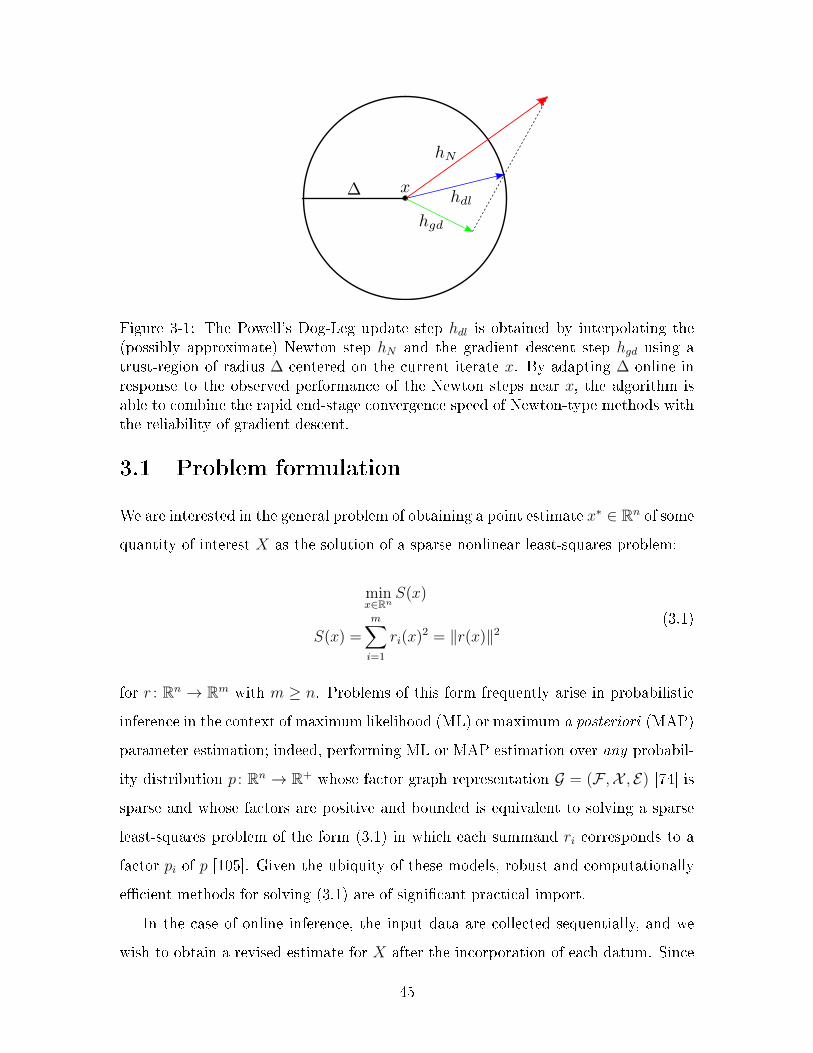
Figure 3-1: The Powell’s Dog-Leg update step ℎ𝑑𝑙 is obtained by interpolating the(possibly approximate) Newton step ℎ𝑁 and the gradient descent step ℎ𝑔𝑑 using atrust-region of radius ∆ centered on the current iterate 𝑥. By adapting ∆ online inresponse to the observed performance of the Newton steps near 𝑥, the algorithm isable to combine the rapid end-stage convergence speed of Newton-type methods withthe reliability of gradient descent.
3.1 Problem formulation
We are interested in the general problem of obtaining a point estimate 𝑥* ∈ R𝑛 of some
quantity of interest 𝑋 as the solution of a sparse nonlinear least-squares problem:
min𝑥∈R𝑛
𝑆(𝑥)
𝑆(𝑥) =𝑚∑𝑖=1
𝑟𝑖(𝑥)2 = ‖𝑟(𝑥)‖2(3.1)
for 𝑟 : R𝑛 → R𝑚 with 𝑚 ≥ 𝑛. Problems of this form frequently arise in probabilistic
inference in the context of maximum likelihood (ML) or maximum a posteriori (MAP)
parameter estimation; indeed, performing ML or MAP estimation over any probabil-
ity distribution 𝑝 : R𝑛 → R+ whose factor graph representation 𝒢 = (ℱ ,𝒳 , ℰ) [74] is
sparse and whose factors are positive and bounded is equivalent to solving a sparse
least-squares problem of the form (3.1) in which each summand 𝑟𝑖 corresponds to a
factor 𝑝𝑖 of 𝑝 [105]. Given the ubiquity of these models, robust and computationally
efficient methods for solving (3.1) are of significant practical import.
In the case of online inference, the input data are collected sequentially, and we
wish to obtain a revised estimate for 𝑋 after the incorporation of each datum. Since
45

each input datum gives rise to a summand in (3.1), online inference corresponds to
solving the sequence of sparse least-squares problems
min𝑥𝑡∈R𝑛𝑡
𝑆(𝑡)(𝑥𝑡)
𝑆(𝑡)(𝑥𝑡) =𝑚𝑡∑𝑖=1
𝑟𝑖 (𝑥𝑖)2 =
𝑟(𝑡)(𝑥𝑡)
2 (3.2)
for 𝑟(𝑡) : R𝑛𝑡 → R𝑚𝑡 and 𝑡 = 1, 2, . . . , where:
1. 𝑚𝑡, 𝑛𝑡 ∈ N+ are monotonically non-decreasing in 𝑡,
2. 𝑥𝑖 ∈ R𝑛𝑖 for all 𝑖 and 𝑥𝑖 ⊆ 𝑥𝑗 for all 𝑖 ≤ 𝑗.
Condition 1 above expresses the fact that the summation in (3.2) evolves over time
only through the addition of new terms. Condition 2 formalizes the idea that we also
allow the vector of states 𝑋 that we wish to estimate to be augmented online by the
addition of new quantities of interest (for example, as in the case of robotic mapping
when exploring previously unseen areas, cf. Fig. 2-1).
Our goal in this chapter is to develop a fully incremental algorithm capable of
robustly solving online sparse least-squares minimization problems of the form (3.2)
in real-time.
3.2 Review of Newton-type optimization methods
and iSAM
The RISE algorithm that we develop in Section 3.4 exploits iSAM’s incremental
computation of the Gauss-Newton step in order to solve the sequential sparse least-
squares problem (3.2) efficiently in the online case. In this section, we review the
general class of Newton-type optimization methods, their specialization to the Gauss-
Newton method, and Gauss-Newton’s incremental implementation in iSAM.
46

3.2.1 Newton’s method and its approximations
Newton’s method [44, 96] is an iterative numerical method for estimating a solution
𝑥* of the general nonlinear minimization problem
min𝑥∈R𝑛
𝑓(𝑥), 𝑓 ∈ 𝐶2(R𝑛). (3.3)
Given an initial estimate 𝑥(𝑖) for 𝑥*, the function 𝑓 is locally approximated at 𝑥(𝑖) by
its second-order Taylor expansion 𝑞(𝑖):
𝑞(𝑖)(𝑥(𝑖) + ℎ) = 𝑓(𝑥(𝑖)) +∇𝑓(𝑥(𝑖))Tℎ+1
2ℎT𝜕2𝑓
𝜕𝑥2(𝑥(𝑖))ℎ, (3.4)
and a revised estimate
𝑥(𝑖+1) = 𝑥(𝑖) + ℎ(𝑖)𝑁 (3.5)
is computed by choosing the Newton step ℎ(𝑖)𝑁 to be any increment to 𝑥(𝑖) that mini-
mizes the value of the local approximation (3.4):
ℎ(𝑖)𝑁 ∈ argmin
ℎ∈R𝑛
𝑞(𝑖)(𝑥(𝑖) + ℎ
). (3.6)
Provided that 𝜕2𝑓𝜕𝑥2 (𝑥(𝑖)) ≻ 0, there is a unique minimizer ℎ(𝑖)𝑁 in (3.6), which is deter-
mined as the solution of
𝜕2𝑓
𝜕𝑥2(𝑥(𝑖))ℎ(𝑖)𝑁 = −∇𝑓(𝑥(𝑖)). (3.7)
Assuming that each of the steps ℎ(𝑖)𝑁 in (3.6) exists, Newton’s method consists of
iteratively applying equations (3.4), (3.6), and (3.5), in that order, to generate a
sequence of estimates 𝑥(0), 𝑥(1), . . . for 𝑥* until some stopping criterion is satisfied.
Newton’s method has several attractive theoretical properties, in particular a fast
(quadratic) convergence rate when initialized with an estimate 𝑥(0) that is close to a
minimizer 𝑥* of a sufficiently regular function 𝑓 [96]. However, in application it may
not always be practical or computationally feasible to evaluate the gradient ∇𝑓(𝑥(𝑖))
47

or Hessian 𝜕2𝑓𝜕𝑥2 (𝑥(𝑖)) in the quadratic model (3.4) at every iteration (depending upon
the dimension 𝑛 and analytical complexity of the function 𝑓). In these cases, the
local model (3.4) is often relaxed to
𝑞(𝑖)(𝑥(𝑖) + ℎ) = 𝑓(𝑥(𝑖)) +(𝑔(𝑖))Tℎ+
1
2ℎT𝐵(𝑖)ℎ, (3.8)
where 𝑔(𝑖) ∈ R𝑛 and 𝐵(𝑖) ∈ R𝑛×𝑛 symmetric are chosen such that
𝑔(𝑖) ≈ ∇𝑓(𝑥(𝑖)), 𝐵(𝑖) ≈ 𝜕2𝑓
𝜕𝑥2(𝑥(𝑖)), (3.9)
and the corresponding update step ℎ(𝑖)𝑁 is computed as a solution of
𝐵(𝑖)ℎ(𝑖)𝑁 = −𝑔(𝑖). (3.10)
The selection of different methods for performing the approximations (3.9) gives rise
to a broad class of optimization algorithms collectively referred to as Newton-type or
approximate Newton methods. With a careful choice of approximation scheme in (3.9)
it is possible to preserve many of the desirable properties of Newton’s method (most
importantly a superlinear end-stage convergence rate) while dramatically reducing
the computational burden of computing the update steps ℎ(𝑖)𝑁 .
3.2.2 The Gauss-Newton method
The Gauss-Newton method [44, 96] is an approximate Newton method for solving the
minimization problem (3.3) in the special case (3.1) in which the objective function
is a sum of squared nonlinear terms. In this case we have
𝜕𝑆
𝜕𝑥𝑗= 2
𝑚∑𝑖=1
𝑟𝑖𝜕𝑟𝑖𝜕𝑥𝑗
, (3.11a)
𝜕2𝑆
𝜕𝑥𝑗𝜕𝑥𝑘= 2
𝑚∑𝑖=1
𝜕𝑟𝑖𝜕𝑥𝑗
𝜕𝑟𝑖𝜕𝑥𝑘
+ 𝑟𝑖𝜕2𝑟𝑖
𝜕𝑥𝑗𝜕𝑥𝑘, (3.11b)
48

and the Gauss-Newton method is obtained as an approximate Newton method by
ignoring the effects of the second-order partial derivatives of 𝑟 when forming the
approximate Hessian 𝐵(𝑖) in (3.9):
𝜕2𝑆
𝜕𝑥𝑗𝜕𝑥𝑘≈ 2
𝑚∑𝑖=1
𝜕𝑟𝑖𝜕𝑥𝑗
𝜕𝑟𝑖𝜕𝑥𝑘
(3.12)
(the exact gradient ∇𝑆(𝑥(𝑖)) corresponding to (3.11a) is used for 𝑔(𝑖)). Using the
function 𝑟 : R𝑛 → R𝑚, we can write this approximation more conveniently in matrix
notation as
𝑔(𝑖) = 2𝐽(𝑥(𝑖))T𝑟(𝑥(𝑖)), (3.13a)
𝐵(𝑖) = 2𝐽(𝑥(𝑖))T𝐽(𝑥(𝑖)), (3.13b)
where 𝐽(𝑥(𝑖)) denotes the Jacobian of 𝑟 evaluated at 𝑥(𝑖):
𝐽(𝑥(𝑖)) =𝜕𝑟
𝜕𝑥
𝑥=𝑥(𝑖)
∈ R𝑚×𝑛. (3.14)
We observe that the approximation (3.12) is equivalent to the assumption that 𝑟
is locally linear. Indeed, substitution of (3.13) into (3.8) produces
𝑞(𝑖)(𝑥(𝑖) + ℎ) = 𝑟(𝑥(𝑖))T𝑟(𝑥(𝑖)) + 2𝑟(𝑥(𝑖))T𝐽(𝑥(𝑖))ℎ
+ ℎT𝐽(𝑥(𝑖))T𝐽(𝑥(𝑖))ℎ
=𝐿(𝑖)(𝑥(𝑖) + ℎ)
2,
(3.15)
where
𝐿(𝑖)(𝑥(𝑖) + ℎ) = 𝑟(𝑥(𝑖)) + 𝐽(𝑥(𝑖))ℎ (3.16)
is the first-order Taylor expansion (i.e. linearization) of 𝑟 about 𝑥(𝑖). Consequently,
by virtue of (3.11b), (3.12), and (3.15), we expect the Gauss-Newton method to
produce the best results when applied to functions 𝑟 that have relatively modest
nonlinearities (as quantified by the magnitudes of their second partial derivatives)
49

and small magnitudes ‖𝑟‖.
To compute the Gauss-Newton step ℎ(𝑖)𝐺𝑁 , we observe that if 𝐽(𝑥(𝑖)) is full-rank,
then 𝐵(𝑖) as defined in (3.13b) is positive definite, and ℎ(𝑖)𝐺𝑁 is determined by
2𝐽(𝑥(𝑖))T𝐽(𝑥(𝑖))ℎ(𝑖)𝐺𝑁 = −2𝐽(𝑥(𝑖))T𝑟(𝑥(𝑖)) (3.17)
following (3.10). Letting
𝑄(𝑖)
⎛⎝𝑅(𝑖)
0
⎞⎠ = 𝐽(𝑥(𝑖)) (3.18)
be a QR decomposition [48] of the Jacobian 𝐽(𝑥(𝑖)) and
⎛⎝𝑑(𝑖)𝑒(𝑖)
⎞⎠ =(𝑄(𝑖)
)T𝑟(𝑥(𝑖)) (3.19)
for 𝑑(𝑖) ∈ R𝑛 and 𝑒(𝑖) ∈ R𝑚−𝑛, we can simplify (3.17) to
𝑅(𝑖)ℎ(𝑖)𝐺𝑁 = −𝑑(𝑖). (3.20)
Since 𝑅(𝑖) is upper-triangular, equation (3.20) can be efficiently solved for ℎ(𝑖)𝐺𝑁 by
back-substitution.
3.2.3 iSAM: Incrementalizing Gauss-Newton
As shown in Section 3.1, the arrival of new data corresponds to augmenting the
function 𝑟 = 𝑟𝑜𝑙𝑑 : R𝑛 → R𝑚 on the right-hand side of (3.1) to the function
𝑟 : R𝑛+𝑛𝑛𝑒𝑤 → R𝑚+𝑚𝑛𝑒𝑤
𝑟 (𝑥𝑜𝑙𝑑, 𝑥𝑛𝑒𝑤) =
⎛⎝ 𝑟𝑜𝑙𝑑 (𝑥𝑜𝑙𝑑)
𝑟𝑛𝑒𝑤 (𝑥𝑜𝑙𝑑, 𝑥𝑛𝑒𝑤)
⎞⎠ ,(3.21)
where here 𝑟𝑛𝑒𝑤 : R𝑛+𝑛𝑛𝑒𝑤 → R𝑚𝑛𝑒𝑤 is the set of new measurement functions and
𝑥𝑛𝑒𝑤 ∈ R𝑛𝑛𝑒𝑤 is the set of new variables introduced as a result of the new observations.
50

In the naïve application of the Gauss-Newton algorithm of Section 3.2.2, the
solution 𝑥* = (𝑥*𝑜𝑙𝑑, 𝑥*𝑛𝑒𝑤) for the augmented least-squares problem determined by
(3.21) would be found by performing Gauss-Newton iterations until convergence.
However, in the context of the sequential estimation problem (3.2) we already have a
good estimate 𝑜𝑙𝑑 for the values of the previously-introduced variables 𝑥𝑜𝑙𝑑, obtained
by solving the least-squares minimization problem (3.1) prior to the introduction of
the new measurement functions 𝑟𝑛𝑒𝑤. Thus, given any good initialization 𝑛𝑒𝑤 for the
newly-introduced system variables 𝑥𝑛𝑒𝑤, = (𝑜𝑙𝑑, 𝑛𝑒𝑤) provides a good initialization
for the augmented state 𝑥 = (𝑥𝑜𝑙𝑑, 𝑥𝑛𝑒𝑤) for the Gauss-Newton algorithm.
Furthermore, since we generally expect the initial estimate to be close to the
true minimizing value 𝑥*, in practice it is not usually necessary to iterate the Gauss-
Newton algorithm until convergence after integration of every new observation; in-
stead, a single Gauss-Newton step is computed and used to correct the initial estimate
. The advantage to this approach is that it avoids having to recompute the Jacobian
𝐽() for 𝑟 and its QR decomposition anew each time new observations arrive; instead,
iSAM efficiently obtains 𝐽() together with its QR decomposition by updating the
Jacobian 𝐽(𝑜𝑙𝑑) and its QR decomposition, as we now describe.
Letting 𝑥 = (𝑥𝑜𝑙𝑑, 𝑥𝑛𝑒𝑤), the Jacobian 𝐽(𝑥) for the augmented system (3.21) can
be decomposed into block form as
𝐽(𝑥) =𝜕𝑟
𝜕𝑥=
⎛⎝ 𝜕𝑟𝑜𝑙𝑑𝜕𝑥𝑜𝑙𝑑
0
𝜕𝑟𝑛𝑒𝑤
𝜕𝑥𝑜𝑙𝑑
𝜕𝑟𝑛𝑒𝑤
𝜕𝑥𝑛𝑒𝑤
⎞⎠ =
⎛⎝𝐽 (𝑥𝑜𝑙𝑑) 0
𝐽𝑛𝑒𝑤(𝑥)
⎞⎠ (3.22)
where
𝐽 (𝑥𝑜𝑙𝑑) =𝜕𝑟𝑜𝑙𝑑𝜕𝑥𝑜𝑙𝑑
∈ R𝑚×𝑛 (3.23)
is the Jacobian of the previous function 𝑟𝑜𝑙𝑑 and
𝐽𝑛𝑒𝑤(𝑥) =𝜕𝑟𝑛𝑒𝑤𝜕𝑥
∈ R𝑚𝑛𝑒𝑤×(𝑛+𝑛𝑛𝑒𝑤) (3.24)
51

is the Jacobian of the new measurement function 𝑟𝑛𝑒𝑤. Letting
𝐽 (𝑜𝑙𝑑) =(𝑄1 𝑄2
)⎛⎝𝑅0
⎞⎠ (3.25)
be a QR decomposition for 𝐽(𝑜𝑙𝑑), where 𝑄1 ∈ R𝑚×𝑛 and 𝑄2 ∈ R𝑚×(𝑚−𝑛), we have
⎛⎝𝑄1 0 𝑄2
0 𝐼 0
⎞⎠⎛⎜⎜⎜⎝
𝑅 0
𝐽𝑛𝑒𝑤()
0
⎞⎟⎟⎟⎠ =
⎛⎝𝑄1𝑅 0
𝐽𝑛𝑒𝑤()
⎞⎠ = 𝐽() (3.26)
by (3.22) and (3.25), which gives a partial QR decomposition of 𝐽(). This partial
decomposition can be completed by using Givens rotations to zero out the remaining
nonzero elements below the main diagonal. Let 𝐺 ∈ R(𝑛+𝑚𝑛𝑒𝑤)×(𝑛+𝑚𝑛𝑒𝑤) denote a
matrix of Givens rotations such that
𝐺
⎛⎝ 𝑅 0
𝐽𝑛𝑒𝑤()
⎞⎠ =
⎛⎝0
⎞⎠ (3.27)
where ∈ R(𝑛+𝑛𝑛𝑒𝑤)×(𝑛+𝑛𝑛𝑒𝑤) is upper-triangular. Defining
=
⎛⎝𝐺 0
0 𝐼
⎞⎠ , =
⎛⎝𝑄1 0 𝑄2
0 𝐼 0
⎞⎠ T, (3.28)
(so that , ∈ R(𝑚+𝑚𝑛𝑒𝑤)×(𝑚+𝑚𝑛𝑒𝑤) are also orthogonal), equations (3.26), (3.27) and
(3.28) show that
𝐽() =
⎛⎝0
⎞⎠ (3.29)
is a QR decomposition for the augmented Jacobian 𝐽(). Now we can use (3.19) and
52

(3.20) to compute the Gauss-Newton step ℎ𝐺𝑁 for the augmented system:
T𝑟() =
⎛⎝𝐺 0
0 𝐼
⎞⎠⎛⎜⎜⎜⎝𝑄T
1 0
0 𝐼
𝑄T2 0
⎞⎟⎟⎟⎠⎛⎝𝑟𝑜𝑙𝑑(𝑜𝑙𝑑)𝑟𝑛𝑒𝑤()
⎞⎠
=
⎛⎝𝐺 0
0 𝐼
⎞⎠⎛⎜⎜⎜⎝
𝑑𝑜𝑙𝑑
𝑟𝑛𝑒𝑤()
𝑒𝑜𝑙𝑑
⎞⎟⎟⎟⎠
=
⎛⎜⎜⎜⎝𝑑
𝑒𝑛𝑒𝑤
𝑒𝑜𝑙𝑑
⎞⎟⎟⎟⎠=
⎛⎝𝑑𝑒
⎞⎠ ,
(3.30)
where ⎛⎝ 𝑑
𝑒𝑛𝑒𝑤
⎞⎠ = 𝐺
⎛⎝ 𝑑𝑜𝑙𝑑
𝑟𝑛𝑒𝑤()
⎞⎠ (3.31)
for 𝑑 ∈ R𝑛+𝑛𝑛𝑒𝑤 . The Gauss-Newton step ℎ𝐺𝑁 used to correct the estimate for the
augmented system is then computed as the solution of
ℎ𝐺𝑁 = −𝑑. (3.32)
Equations (3.24), (3.27) and (3.31) show how to obtain the factor of the QR
decomposition of 𝐽() and the corresponding linear system (3.32) by updating the
𝑅 factor and linear system for the previous Jacobian 𝐽(𝑜𝑙𝑑) using Givens rotations.
Since the updated factor and the new right-hand side vector 𝑑 are obtained by
applying 𝐺 directly to the augmented factor 𝑅 in (3.27) and the augmented right-
hand side vector 𝑑 in (3.31), it is not necessary to explicitly form the orthogonal matrix
in (3.28). Nor is it necessary to form the matrix 𝐺 explicitly either; instead, the
appropriate individual Givens rotations can be applied sequentially directly to the
53

matrix in (3.27) and the right-hand side vector in (3.31). Under the assumption of
sparsity, only a few elements of the the Jacobian 𝐽𝑛𝑒𝑤() will be nonzero, and therefore
only a small number of Givens rotations will be needed to perform the update in
(3.27). Obtaining the linear system (3.32) by this method is thus a computationally
efficient operation.
Finally, we observe that while relinearization is not needed after every new ob-
servation, the system should be periodically relinearized about its corrected estimate
in order to perform a full Gauss-Newton iteration and obtain a better estimate of
the local minimum (this is particularly true after observations which are likely to
significantly alter the estimates of system variables). When relinearizing the system
about the corrected estimate, the incremental updating method outlined above is
no longer applicable; instead, the QR factorization of the Jacobian needs to be re-
computed anew. While this is an expensive batch operation, the factorization step
can be combined with a variable reordering step [32] in order to reduce the fill-in
in the resulting factor 𝑅, thereby maintaining sparsity and speeding up subsequent
incremental computations.
3.3 From Gauss-Newton to Powell’s Dog-Leg
The incrementalized Gauss-Newton method outlined in Section 3.2.3 is computation-
ally efficient, straightforward to implement, and enjoys rapid (up to quadratic [44,
pg. 113]) convergence near the minimum. However, the assumption of the local lin-
earity of 𝑟 (which underlies the approximations (3.13b) and (3.15)) means that the
Gauss-Newton method can exhibit poor behavior when either 𝑟 itself or its second
partial derivatives 𝜕2𝑟𝜕𝑥𝑗𝜕𝑥𝑘
have large magnitude. Indeed, convergence of the Gauss-
Newton method is not guaranteed, not even locally ; this is in marked contrast with
the behavior of Newton’s method, which (although not globally convergent) can at
least guarantee fast local convergence for a class of functions that is not excessively
restrictive in practice (cf. Theorem 3.5 of [96]). Furthermore, it is not difficult to
construct simple (even quadratic) examples of 𝑟 where the sequence of Gauss-Newton
54

iterates 𝑥(𝑖)∞𝑖=1 is in fact globally divergent (i.e. fails to converge when initialized at
any point 𝑥(0) = 𝑥*).
As a concrete example, consider the minimization (3.1) determined by:
𝑟 : R→ R2
𝑟(𝑥) =
⎛⎝ 𝑥+ 1
𝜆𝑥2 + 𝑥− 1
⎞⎠ .(3.33)
For 𝜆 = −2, the function 𝑆(𝑥) is 𝐶∞ and strictly convex, and has a single global
minimum at 𝑥* = 0 (cf. Fig. 3-2(a)), hence satisfies all of the standard regularity
conditions customarily assumed in numerical optimization (cf. e.g. [44, 96]). Never-
theless, the Gauss-Newton algorithm is in fact globally divergent when applied to this
function [44, pg. 113]. Fig. 3-2(b) shows the distance from the 𝑖th Gauss-Newton iter-
ate 𝑥(𝑖) to the global minimizer 𝑥* for the first 100 iterations of a sequence initialized
with 𝑥(0) = 10−4. Note that the Gauss-Newton method initially drives the estimate
𝑥(𝑖) away from the global minimum 𝑥* before converging to a 6-periodic orbit. To see
why this is so, Fig. 3-2(c) illustrates the behavior of the Gauss-Newton update rule
𝐺𝑁 : 𝑥(𝑖) ↦→ 𝑥(𝑖+1) and its 6-fold composition 𝐺𝑁 (6) considered as dynamical systems
on R. Note that the graph of 𝐺𝑁 intersects the graph of the identity mapping at the
minimizer 𝑥* = 0, showing that 𝑥* is a fixed point of 𝐺𝑁 (as we would hope); however
∇𝐺𝑁(𝑥*) = −2, so that |∇𝐺𝑁(𝑥*) − 1| = 3 > 1, and therefore this fixed point is
repelling [121, Chp. 10]. The intersections of the graph of 𝐺𝑁 (6) with the graph of
the identity mapping give the 6-periodic points of 𝐺𝑁 , including the members of the
6-periodic orbit to which the Gauss-Newton iterates converge in Fig. 3-2(b). This
lack of robustness even under ideal conditions (viz. a well-behaved objective function
with strong regularity properties and good initialization) is a serious shortcoming of
the Gauss-Newton method.
To address this shortcoming, in this chapter we adopt the Powell’s Dog-Leg al-
gorithm [96, 101] as the method of choice for performing the sparse least-squares
minimization (3.1). This algorithm combines the superlinear end-stage convergence
55

−1.5 −1 −0.5 0 0.5 1 1.50
10
20
30
40
Objective function S(x)
x
S(x
)
(a) The objective function 𝑆(𝑥)
0 20 40 60 80 1000
0.1
0.2
0.3
0.4
0.5
0.6
0.7
Gauss−Newton iterations
Iteration
Dis
tance to m
inim
izer
(b) Gauss-Newton iterates
−1 −0.5 0 0.5 1
−1
−0.5
0
0.5
1
Current iterate
Ne
xt
ite
rate
Gauss−Newton dynamical system
GN
GN(6)
Identity
(c) Gauss-Newton dynamical system
0 2 4 6 8 10 120
0.2
0.4
0.6
0.8
1
IGN−PDL iterations
Iteration
Dis
tan
ce
to
min
imiz
er
(d) IGN-PDL iterates
Figure 3-2: Failure of the Gauss-Newton method. (a): The graph of the sum-of-squares objective function 𝑆(𝑥) determined by (3.33) for 𝜆 = −2. (b): This plotshows the distance from the 𝑖th Gauss-Newton iterate 𝑥(𝑖) to the global minimizer𝑥* of (a) for the first 100 iterations of a sequence initialized with 𝑥(0) = 10−4. (c):This figure plots the Gauss-Newton update rule 𝐺𝑁 : 𝑥(𝑖) ↦→ 𝑥(𝑖+1) and its 6-foldcomposition 𝐺𝑁 (6) considered as dynamical systems on R. (d): This plot showsthe distance from the 𝑖th IGN-PDL iterate 𝑥(𝑖) to the minimizer 𝑥* for 20 sequenceswith initializations 𝑥(0) sampled uniformly randomly from [−1, 1] and parameters∆(0) = .01, 𝜂1 = .25, 𝜂2 = .75, 𝛾1 = .5, 𝛾2 = 2. The 12th iterates 𝑥(12) of thesesequences are all within 3 × 10⁻⁴ of the minimizer 𝑥*. Strong global convergenceproperties and robustness to highly nonlinear and ill-conditioned systems are generalfeatures of this algorithm (cf. Sec. 3.3.4).
56

speed of Newton-type methods with the excellent global convergence properties of
gradient descent approaches [28, 102, 113]. Indeed, when applied to sparse least-
squares minimization problems, Powell’s Dog-Leg performs significantly faster than
Levenberg-Marquardt (the current method of choice in the robotics and computer
vision communities) while maintaining comparable levels of accuracy [83].
3.3.1 The trust-region approach
As shown in Section 3.2.1, in each iteration Newton’s method constructs a local model
𝑞(𝑖) for the objective function 𝑓 on a neighborhood 𝑈 (𝑖) of the current estimate 𝑥(𝑖),
and then determines an update step ℎ(𝑖)𝑁 that minimizes 𝑞(𝑖) in place of 𝑓 . However,
the model 𝑞(𝑖) in (3.4) is constructed using information about 𝑓 ’s first- and second-
order derivatives at 𝑥(𝑖), which depend only upon the local behavior of 𝑓 near 𝑥(𝑖).
Consequently, while 𝑞(𝑖) is a good approximation of 𝑓 near 𝑥(𝑖) (in a sense made precise
by Taylor’s Theorem), its global behavior may be quite different from 𝑓 ’s. This can
become problematic if the update step ℎ(𝑖)𝑁 computed using 𝑞(𝑖) leaves the region 𝑈 (𝑖)
in which 𝑓 is well-approximated by 𝑞(𝑖).
Trust-region methods [96] address this hazard by maintaining an explicit trust-
region, an open ball of radius ∆(𝑖) centered on the current estimate 𝑥(𝑖) within which
𝑓 is considered well-approximated by the local model 𝑞(𝑖). The trust-region update
step ℎ(𝑖)𝑡𝑟 is then obtained as an increment to 𝑥(𝑖) that minimizes the value of 𝑞(𝑖),
subject to the condition that the update step does not leave the trust-region:
ℎ(𝑖)𝑡𝑟 ∈ argmin
‖ℎ‖≤Δ(𝑖)
𝑞(𝑖)(𝑥(𝑖) + ℎ). (3.34)
The following theorem gives necessary and sufficient optimality conditions char-
acterizing the trust-region step ℎ(𝑖)𝑡𝑟 in (3.34) when 𝑞(𝑖) is a quadratic model (as in
approximate Newton methods). Its proof follows from a straightforward application
of the Karush-Kuhn-Tucker first- and second-order necessary optimality conditions
(cf. [96, Chps. 4 and 12]).
57

Theorem 1 (Optimality conditions for the trust-region step). Let 𝑓, 𝑔 ∈ R𝑛, let
𝐵 ∈ R𝑛×𝑛 be symmetric, and define
𝑞 : R𝑛 → R
𝑞(ℎ) = 𝑓 + 𝑔Tℎ+1
2ℎT𝐵ℎ.
(3.35)
Then ℎ* ∈ R𝑛 is a solution of the constrained minimization
minℎ∈R𝑛
𝑞(ℎ) s.t. ‖ℎ‖ ≤ ∆ (3.36)
for ∆ > 0 if and only if ‖ℎ*‖ ≤ ∆ and there exists 𝜆* ≥ 0 such that the following
conditions are satisfied:
(𝐵 + 𝜆*𝐼)ℎ* = −𝑔, (3.37a)
𝜆*(∆− ‖ℎ*‖) = 0, (3.37b)
(𝐵 + 𝜆*𝐼) ⪰ 0. (3.37c)
As the trust-region method proceeds, the radius of the trust region ∆(𝑖) is varied
adaptively according to the gain ratio:
𝜌(𝑖) =ared(𝑖)(ℎ
(𝑖)𝑡𝑟 )
pred(𝑖)(ℎ(𝑖)𝑡𝑟 )
, (3.38)
where
ared(𝑖)(ℎ(𝑖)𝑡𝑟 ) = 𝑓(𝑥(𝑖))− 𝑓(𝑥(𝑖) + ℎ
(𝑖)𝑡𝑟 ),
pred(𝑖)(ℎ(𝑖)𝑡𝑟 ) = 𝑞(𝑖)(𝑥(𝑖))− 𝑞(𝑖)(𝑥(𝑖) + ℎ
(𝑖)𝑡𝑟 );
(3.39)
this compares the actual reduction in the objective function’s value obtained by taking
the proposed trust-region step ℎ(𝑖)𝑡𝑟 with the predicted reduction in function value
using the local model 𝑞(𝑖). Values of 𝜌 close to 1 indicate that the local model 𝑞(𝑖) is
performing well near the current iterate 𝑥(𝑖), so the trust-region radius ∆(𝑖) can be
increased in the next iteration (to allow longer steps and hence faster convergence),
58

Algorithm 3.1 Updating the trust-region radius ∆
1: function Update_Delta(𝜌, ∆, 𝜂1, 𝜂2, 𝛾1, 𝛾2)2: if 𝜌 ≥ 𝜂2 then3: ∆← 𝛾2∆4: else if 𝜌 < 𝜂1 then5: ∆← 𝛾1∆6: end if
7: return ∆8: end function
Algorithm 3.2 The trust-region minimization method1: function Trust-region(𝑓 , 𝑥0, ∆0, 𝜂1, 𝜂2, 𝛾1, 𝛾2)2: Initialize 𝑥← 𝑥0, ∆← ∆0.3: repeat
4: Construct local model 𝑞 for 𝑓 about 𝑥.5: Compute trust-region step ℎ𝑡𝑟 by solving (3.34).6: Set 𝑥𝑝𝑟𝑜𝑝𝑜𝑠𝑒𝑑 ← (𝑥+ ℎ𝑡𝑟).7: Compute 𝜌 using (3.38).8: if 𝜌 ≥ 𝜂1 then9: Set 𝑥← 𝑥𝑝𝑟𝑜𝑝𝑜𝑠𝑒𝑑.10: end if
11: ∆← Update_Delta(𝜌, ∆, 𝜂1, 𝜂2, 𝛾1, 𝛾2).12: until (stopping criteria)13: return 𝑥14: end function
while values close to 0 indicate that the local model is performing poorly, and ∆(𝑖)
should be reduced accordingly (Algorithm 3.1). The entire trust-region method is
summarized as Algorithm 3.2; here 0 < 𝜂1 < 𝜂2 < 1 and 0 < 𝛾1 < 1 < 𝛾2 are user-
supplied parameters specifying the gain-ratio thresholds and scaling factors used in
the update of the trust-region radius.
3.3.2 Powell’s Dog-Leg
While the canonical trust-region method (Algorithm 3.2) is intellectually pleasing and
enjoys excellent convergence and robustness properties (cf. Section 3.3.4), it is not
commonly used in practice because of the computational cost of finding the exact
trust-region step ℎ𝑡𝑟 in (3.34). (Briefly, this entails solving a root-finding problem
for the Lagrange multiplier 𝜆* in (3.37a) that generally requires multiple factoriza-
59

tions of matrices of the form 𝐵 + 𝜆𝐼 [93], a prohibitively expensive operation when
appearing as a single step within another iterative algorithm.) Instead, most practi-
cal trust-region implementations solve (3.34) approximately using a computationally
cheap approximation that is nevertheless accurate enough to preserve the desirable
properties of the canonical algorithm. In this section we describe Powell’s Dog-Leg
[96, 101], one such approximate method that can be used whenever the matrix 𝐵 in
the local quadratic model 𝑞 in (3.34) is positive definite.
The dog-leg approximation is derived by regarding the trust-region step computed
in (3.34) as a function ℎ𝑡𝑟(∆) of the trust-region radius and considering the effect of
varying ∆. For 𝐵 ∈ R𝑛×𝑛 symmetric and positive definite, the local model 𝑞 has a
unique unconstrained minimizer: the Newton step
ℎ𝑁 = −𝐵−1𝑔. (3.40)
If the trust-region radius ∆ is greater than the length of this step, then the constraint
in (3.34) is inactive, and therefore
ℎ𝑡𝑟(∆) = ℎ𝑁 , ‖ℎ𝑁‖ ≤ ∆. (3.41)
Conversely, when the trust-region radius ∆ is small, the (second-order) quadratic
term in the local model (3.8) is dominated by the linear term, and therefore the
trust-region step computed in (3.34) will be well-approximated by the maximum step
length allowable in the direction of steepest descent:
ℎ𝑡𝑟(∆) ≈ − ∆
‖𝑔‖𝑔, ∆ small. (3.42)
As ∆ increases through the range [0,∞), the exact trust-region step ℎ𝑡𝑟(∆) traces a
smooth path interpolating these cases; Powell’s Dog-Leg approximates this path using
a piecewise linear path with two segments (Fig. 3-3). The first segment extends from
𝑥 to the gradient descent step ℎ𝑔𝑑, which we define as the unconstrained minimizer
60

x0
x*
Trust−region and dog−leg paths
−3 −2 −1 0 1 2−3
−2
−1
0
1
2
3
Model contours
Trust−region path
Dog−leg path
Figure 3-3: This figure shows the trust-region and Powell’s Dog-Leg paths for aquadratic model 𝑞 constructed at 𝑥0 with minimizer 𝑥*. As the trust-region ra-dius ∆ increases, the trust-region step ℎ𝑡𝑟(∆) traces a smooth path interpolating theconstrained gradient descent step and the Newton step ℎ𝑁 . Powell’s Dog-Leg approx-imates this path using a piecewise linear path with two segments: the first from 𝑥0to the full gradient descent step ℎ𝑔𝑑, and the second from ℎ𝑔𝑑 to the Newton step ℎ𝑁 .
of the local model 𝑞 along the steepest descent direction:
ℎ𝑔𝑑 = −𝛼𝑔, 𝛼 = argmin𝑎∈R+
𝑞(𝑥− 𝑎𝑔). (3.43)
Using the definition of the local model (3.8) and the fact that 𝐵 ≻ 0 by hypothesis,
the gradient descent step defined in (3.43) can be written in closed form as:
ℎ𝑔𝑑 = −𝛼𝑔, 𝛼 =𝑔T𝑔
𝑔T𝐵𝑔. (3.44)
The second segment linearly interpolates the gradient descent step ℎ𝑔𝑑 and the Newton
step ℎ𝑁 . Parameterizing the dog-leg path as 𝑝𝑑𝑙 : [0, 1]→ R𝑛, we have
𝑝𝑑𝑙(𝑡) =
⎧⎪⎨⎪⎩2𝑡ℎ𝑔𝑑, 0 ≤ 𝑡 ≤ 12,
ℎ𝑔𝑑 + (2𝑡− 1)(ℎ𝑁 − ℎ𝑔𝑑), 12≤ 𝑡 ≤ 1.
(3.45)
A direct computation using the definitions (3.40), (3.43), and (3.45) proves the
following result (cf. e.g. [96, Sec. 4.1]).
61

Lemma 2. The dog-leg path 𝑝𝑑𝑙 defined in (3.45) satisfies the following properties:
(i) ‖𝑝𝑑𝑙(𝑡)‖ is monotonically increasing for all 𝑡 ∈ [0, 1].
(ii) 𝑞(𝑝𝑑𝑙(𝑡)) is monotonically decreasing for all 𝑡 ∈ [0, 1].
By virtue of Lemma 2, the Powell’s Dog-Leg step ℎ𝑑𝑙 is defined to be the (unique)
farthest point along the dog-leg path 𝑝𝑑𝑙 lying inside the trust-region boundary (cf.
Fig. 3-1):
ℎ𝑑𝑙 = 𝑝𝑑𝑙(𝜏),
𝜏 = max 𝑡 ∈ [0, 1] | ‖𝑝𝑑𝑙(𝑡)‖ ≤ ∆ .(3.46)
The algorithmic computation of the dog-leg step ℎ𝑑𝑙 corresponding to definition (3.46)
is given in Algorithm 3.3. The scalar 𝛽 appearing in line 7 is chosen to satisfy
‖ℎ𝑔𝑑 + 𝛽(ℎ𝑁 − ℎ𝑔𝑑)‖2 = ∆2, (3.47)
which is quadratic in 𝛽. By Lemma 2, (3.47) has exactly one solution in (0, 1), which
can be written in closed form as
𝑣 = ℎ𝑁 − ℎ𝑔𝑑,
𝛽 =−ℎT𝑔𝑑𝑣 +
√(ℎT𝑔𝑑𝑣)2 + (∆2 − ‖ℎ𝑔𝑑‖2)‖𝑣‖2
‖𝑣‖2.
(3.48)
The complete Powell’s Dog-Leg algorithm is obtained from Algorithm 3.2 by re-
placing the computation of the trust-region step ℎ𝑡𝑟 in line 5 with the computation
of the dog-leg step ℎ𝑑𝑙 defined by equations (3.40), (3.44), and Algorithm 3.3.
3.3.3 Indefinite Gauss-Newton-Powell’s Dog-Leg
In this subsection we derive an approximate trust-region algorithm based on Powell’s
Dog-Leg with Gauss-Newton steps for solving problems of the form (3.1).
To begin, we observe that by virtue of the Hessian approximations (3.13b) used
in the Gauss-Newton local model 𝑞, 𝐵 ⪰ 0 always. If 𝐽(𝑥) is full-rank, then 𝐵 ≻ 0
62

Algorithm 3.3 Computing the dog-leg step ℎ𝑑𝑙1: function Compute_Dog-Leg(ℎ𝑁 , ℎ𝑔𝑑, ∆)2: if ‖ℎ𝑁‖ ≤ ∆ then
3: ℎ𝑑𝑙 ← ℎ𝑁4: else if ‖ℎ𝑔𝑑‖ ≥ ∆ then
5: ℎ𝑑𝑙 ←(
Δ‖ℎ𝑔𝑑‖
)ℎ𝑔𝑑
6: else
7: ℎ𝑑𝑙 ← ℎ𝑔𝑑 + 𝛽 (ℎ𝑁 − ℎ𝑔𝑑), where 𝛽 ∈ (0, 1) is chosen such that ‖ℎ𝑑𝑙‖ = ∆(cf. equation (3.48)).
8: end if
9: return ℎ𝑑𝑙10: end function
and the dog-leg step ℎ𝑑𝑙 defined in Section 3.3.2 exists and can be computed in terms
of the Gauss-Newton step ℎ𝐺𝑁 and the gradient descent step ℎ𝑔𝑑. Equations (3.18)–
(3.20) already provide a closed-form solution for computing the Gauss-Newton step,
so it suffices to provide a closed-form solution for the gradient descent step ℎ𝑔𝑑 in
(3.44). Substituting the expressions for 𝐵 and 𝑔 from (3.13) into (3.44), we find
𝑔 = 2𝐽(𝑥)T𝑟(𝑥), 𝛼 =‖𝑔‖2
2‖𝐽(𝑥)𝑔‖2. (3.49)
Equations (3.18)–(3.20), (3.49), and Algorithm 3.3 thus enable the computation
of the dog-leg step ℎ𝑑𝑙 when 𝐵 ≻ 0.
In the case that 𝐽(𝑥) is not full-rank, 𝐵 is not positive definite and the dog-leg
step is not defined. However, the Cauchy step ℎ𝐶 (the constrained minimizer of the
local model 𝑞 along the steepest descent direction):
ℎ𝐶 = −𝜅𝑔
𝜅 = argmin0≤𝑎≤ Δ
‖𝑔‖
𝑞(𝑥− 𝑎𝑔)(3.50)
always exists and is unique for 𝑔 = 0 and arbitrary symmetric 𝐵 ∈ R𝑛×𝑛 in the local
model (3.8). Indeed, direct computation in (3.50) shows that the step-length 𝜅 can
63

be written in a simple closed form as:
𝜅 =
⎧⎪⎨⎪⎩min
Δ‖𝑔‖ ,
‖𝑔‖2𝑔T𝐵𝑔
, 𝑔T𝐵𝑔 > 0,
Δ‖𝑔‖ , 𝑔T𝐵𝑔 ≤ 0.
(3.51)
Substituting the approximate Hessian (3.13b) from the Gauss-Newton local model
into (3.51) produces:
𝜅 =
⎧⎪⎨⎪⎩min
Δ‖𝑔‖ ,
‖𝑔‖22‖𝐽(𝑥)𝑔‖2
, ‖𝐽(𝑥)𝑔‖ > 0,
Δ‖𝑔‖ , ‖𝐽(𝑥)𝑔‖ = 0.
(3.52)
Our proposed algorithm, which we refer to as the indefinite Gauss-Newton-Powell’s
Dog-Leg (IGN-PDL) algorithm, is obtained from Algorithm 3.2 by using Gauss-
Newton-Powell’s Dog-Leg steps in line 5 when 𝐽(𝑥) is full-rank, and constrained
Cauchy steps otherwise.
Finally, for the sake of notational simplicity and to avoid unnecessary work, we
simplify the computations in (3.49) and (3.52) by canceling the common factors of 2
in the gradient vector 𝑔 and the stepsizes 𝛼 and 𝜅. This produces
𝑔 = 𝐽(𝑥)T𝑟(𝑥), (3.53a)
𝛼 =‖𝑔‖2
‖𝐽(𝑥)𝑔‖2, (3.53b)
𝜅 =
⎧⎪⎨⎪⎩min
Δ‖𝑔‖ ,
‖𝑔‖2‖𝐽(𝑥)𝑔‖2
, ‖𝐽(𝑥)𝑔‖ > 0,
Δ‖𝑔‖ , ‖𝐽(𝑥)𝑔‖ = 0.
(3.53c)
The IGN-PDL algorithm is summarized as Algorithm 3.4.
3.3.4 Analysis of the IGN-PDL algorithm
While the trust-region approach of Section 3.3.1 may appear to be only a slight vari-
ation on the Newton-type methods, in fact trust-region algorithms possess markedly
superior robustness properties. In this subsection we examine two such properties
64

Algorithm 3.4 The indefinite Gauss-Newton-Powell’s Dog-Leg algorithm1: function IGN-PDL(𝑟, 𝑥0, ∆0, 𝜂1, 𝜂2, 𝛾1, 𝛾2)2: Initialize 𝑥← 𝑥0, ∆← ∆0.3: repeat
4: Set 𝑔 ← 𝐽(𝑥)T𝑟(𝑥).5: Compute 𝑅 factor and right-hand side vector 𝑑
as in equations (3.18) and (3.19).6: if 𝑅 is nonsingular then7: Compute Gauss-Newton step ℎ𝐺𝑁 using (3.20).8: Set 𝛼← ‖𝑔‖2/‖𝐽(𝑥)𝑔‖2.9: Set ℎ𝑔𝑑 ← −𝛼𝑔.10: Set ℎ←Compute_Dog-Leg(ℎ𝐺𝑁 , ℎ𝑔𝑑, ∆).11: else
12: Compute 𝜅 using equation (3.53c).13: Set ℎ← −𝜅𝑔.14: end if
15: Set 𝑥𝑝𝑟𝑜𝑝𝑜𝑠𝑒𝑑 ← (𝑥+ ℎ).16: Compute 𝜌 using (3.38).17: if 𝜌 ≥ 𝜂1 then18: Set 𝑥← 𝑥𝑝𝑟𝑜𝑝𝑜𝑠𝑒𝑑.19: end if
20: ∆← Update_Delta(𝜌, ∆, 𝜂1, 𝜂2, 𝛾1, 𝛾2).21: until (stopping criteria)22: return 𝑥23: end function
(global convergence and robustness to numerical ill-conditioning), and prove a strong
global convergence result for the IGN-PDL algorithm of Section 3.3.3.
Global convergence
One of the most attractive and powerful features of trust-region algorithms is that
they are globally convergent under very general conditions, even when using (possibly
very loose) gradient and Hessian approximations in the local models 𝑞(𝑖). By way of
illustration, the following remarkable theorem is due to R.G. Carter [28].
Theorem 3 (Global convergence of trust-region methods). Let 𝑓 : R𝑛 → R, 𝑥(0) ∈
R𝑛, and let Ω ⊆ R𝑛 be any convex open set containing the sublevel set ℒ𝑓 (𝑥(0)) of 𝑓
at 𝑥(0):
ℒ𝑓 (𝑥(0)) =𝑥 ∈ R𝑛 | 𝑓(𝑥) ≤ 𝑓(𝑥(0))
. (3.54)
65

Assume further that 𝑓 is lower-bounded on Ω, 𝑓 ∈ 𝐶1(Ω), and that ∇𝑓 is Lipschitz
continuous on Ω.
Fix constants 0 < 𝜂1 < 𝜂2 < 1 and 0 < 𝛾1 < 1 < 𝛾2, 𝜁 < 1 − 𝜂2, 𝛽, 𝜎 ∈ (0,∞), and
𝑐 ∈ (0, 1], and let 𝑥(𝑖)∞𝑖=0 be the sequence of iterates obtained in Algorithm 3.2 using
local models 𝑞(𝑖) and approximate trust-region update steps ℎ(𝑖)𝑡𝑟 in line 5 that satisfy
the following criteria:
(i) Feasibility: ‖ℎ(𝑖)𝑡𝑟 ‖ ≤ ∆(𝑖) for all 𝑖 ≥ 0.
(ii) Gradient approximation error: the approximate gradients 𝑔(𝑖) used in each of
the local models 𝑞(𝑖) satisfy the bounded relative error criterion:
‖𝑔(𝑖) −∇𝑓(𝑥(𝑖))‖‖𝑔(𝑖)‖
≤ 𝜁. (3.55)
(iii) Uniform boundedness of approximate Hessians: each 𝐵(𝑖) ∈ R𝑛×𝑛 is symmetric
and satisfies ‖𝐵(𝑖)‖ ≤ 𝛽.
(iv) Asymptotic step direction: assuming that ‖𝐵(𝑖)‖ ≤ 𝛽 for all 𝑖 ≥ 0 and that
lim inf𝑖→∞
‖𝑔(𝑖)‖ > 0 and lim𝑖→∞
∆(𝑖) = 0, (3.56)
the step direction Θ(𝑖) satisfies
lim𝑖→∞
cos Θ(𝑖) = 1, (3.57)
where
cos Θ(𝑖) = −(𝑔(𝑖))Tℎ(𝑖)𝑡𝑟
‖𝑔(𝑖)‖‖ℎ(𝑖)𝑡𝑟 ‖. (3.58)
(v) Uniform predicted decrease: each of the proposed update steps ℎ(𝑖)𝑡𝑟 satisfies:
pred(𝑖)(ℎ(𝑖)𝑡𝑟 ) ≥ 1
2𝑐‖𝑔(𝑖)‖min
∆(𝑖),
‖𝑔(𝑖)‖𝜎
. (3.59)
66
Then either ∇𝑓(𝑥(𝑖)) = 0 for some iterate 𝑥(𝑖), or the infinite subsequence 𝑥(𝑖𝑘)∞𝑘=0 ⊆
𝑥(𝑖)∞𝑖=0 of iterates that are accepted in line 9 of Algorithm 3.2 satisfies
lim𝑘→∞‖∇𝑓(𝑥(𝑖𝑘))‖ = 0. (3.60)
With the aid of Theorem 3, we prove the following convergence result for the
IGN-PDL algorithm (Algorithm 3.4).
Theorem 4 (Global convergence of the IGN-PDL algorithm). Let 𝑟 : R𝑛 → R𝑚 be
𝐶2, define
𝑆(𝑥) = ‖𝑟(𝑥)‖2, (3.61)
and fix 0 < 𝜂1 < 𝜂2 < 1 and 0 < 𝛾1 < 1 < 𝛾2. Given any 𝑥(0) ∈ R𝑛, if the sublevel
set ℒ𝑆(𝑥(0)) is bounded, then the sequence 𝑥(𝑖) of iterates accepted in line 18 of
Algorithm 3.4 either terminates at some 𝑥(𝑘) with ∇𝑆(𝑥(𝑘)) = 0 or satisfies
lim𝑖→∞‖∇𝑆(𝑥(𝑖))‖ → 0. (3.62)
This theorem is proved in Appendix A.
In practice, the hypotheses of Theorem 4 are quite general; intuitively, the bounded
sublevel set condition simply prohibits the cost function 𝑆 from assigning the same
quality to arbitrarily large regions of the state space. Any reasonable inferential cost
function arising in practice will satisfy this condition.
Robustness to numerical ill-conditioning
In addition to their strong convergence properties, trust-region methods are also nat-
urally robust against numerical ill-conditioning in the linear system (3.10) used to
solve for the Newton step.
Recall that for a matrix 𝐴 ∈ R𝑚×𝑛 with 𝑚 ≥ 𝑛, the condition number 𝜅2(𝐴) (cf.
[48, pg. 230]) is
𝜅2(𝐴) =
⎧⎪⎨⎪⎩𝜎max(𝐴)𝜎min(𝐴)
, rank(𝐴) = 𝑛,
∞, rank(𝐴) < 𝑛,
(3.63)
67
where 𝜎max(𝐴) and 𝜎min(𝐴) give the maximum and minimum singular values of 𝐴,
respectively. Matrices 𝐴 with 𝜅2(𝐴) ≫ 1 are called ill-conditioned ; these matrices
tend to have poor numerical properties when used as the coefficient matrix for inverse
problems of the form
min𝑥∈R𝑛‖𝐴𝑥− 𝑏‖2 (3.64)
for 𝑏 ∈ R𝑚 (of which (3.10) and (3.15) are special cases). To see why this is so,
observe that if rank(𝐴) = 𝑛, then (3.64) has the unique minimizer
𝑥𝐿𝑆 = argmin𝑥∈R𝑛
‖𝐴𝑥− 𝑏‖2 =𝑛∑
𝑖=1
𝑢T𝑖 𝑏
𝜎𝑖𝑣𝑖, (3.65)
where 𝜎1 ≥ · · · ≥ 𝜎𝑛 > 0 are the singular values of 𝐴, and 𝑢𝑖 ∈ R𝑚×1 and 𝑣𝑖 ∈ R𝑛×1 are
the left- and right-singular vectors (respectively) corresponding to 𝜎𝑖 for all 1 ≤ 𝑖 ≤ 𝑛
(cf. [48, Sec. 5.5.3]). If 𝜅2(𝐴)≫ 1, then since 𝑢𝑖𝑛𝑖=1 and 𝑣𝑖𝑛𝑖=1 are orthonormal sets,
(3.65) shows that 𝑥𝐿𝑆 will tend to be dominated by the effects of those (generally few)
components of 𝑏 lying in subspaces spanned by left-singular vectors 𝑢𝑖 corresponding
to small singular values 𝜎𝑖. In practice, this commonly manifests as the least-squares
solution 𝑥𝐿𝑆 “exploding” (as measured by ‖·‖) through subspaces of R𝑛 spanned by
right-singular vectors 𝑣𝑖 corresponding to small singular values 𝜎𝑖 whenever 𝐴 is ill-
conditioned.
One standard approach for addressing poor numerical conditioning in (3.64) is
Tikhonov regularization [132]. In this approach, problem (3.64) is replaced by
min𝑥∈R𝑛‖𝐴𝑥− 𝑏‖2 + 𝜆‖Γ𝑥‖2, (3.66)
where Γ ∈ R𝑛×𝑛 is a conditioning matrix designed to control some property of interest
of the Tikhonov-regularized solution, and 𝜆 ≥ 0 is a parameter controlling the applied
degree of regularization. The minimizer 𝑥𝜆 of (3.66) can be formally computed in
68

closed form as
𝑥𝜆 = argmin𝑥∈R𝑛
‖𝐴𝑥− 𝑏‖2 + 𝜆‖Γ𝑥‖2
= (𝐴T𝐴+ 𝜆ΓTΓ)−1𝐴T𝑏.
(3.67)
The standard form of Tikhonov regularization has Γ = 𝐼, which simply controls
the norm of 𝑥𝜆. More interestingly, this choice also has the effect of improving the
numerical conditioning of (3.66) versus (3.64). To see this, observe that (3.66) with
Γ = 𝐼 can be expressed as an instance of (3.64):
min𝑥∈R𝑛‖𝐴𝑥− 𝑏‖2 + 𝜆‖𝑥‖2 = min
𝑥∈R𝑛
𝐴𝑥−
2, (3.68)
where
𝐴 =
⎛⎝ 𝐴√𝜆𝐼
⎞⎠ , =
⎛⎝𝑏0
⎞⎠ . (3.69)
The 𝑛×𝑛 block√𝜆𝐼 of the augmented coefficient matrix 𝐴 ensures that 𝜎min(𝐴) ≥
√𝜆, and the Pythagorean theorem implies that 𝜎max(𝐴) = ‖𝐴‖ ≤
√𝜆+ ‖𝐴‖2. These
two inequalities together imply that
𝜅2(𝐴) ≤√𝜆+ ‖𝐴‖2√
𝜆=
√1 +‖𝐴‖2𝜆
. (3.70)
Equation (3.70) shows that the regularization parameter 𝜆 controls the effective con-
ditioning of the Tikhonov-regularized system (3.66)–(3.69) when Γ = 𝐼.
We now highlight a remarkable connection between trust-region methods and
Tikhonov regularization. Consider the optimality condition (3.37a) for the trust-
region step in Theorem 1, and suppose that 𝐵 ⪰ 0. Since 𝐵 is symmetric, it can be
diagonalized by an orthogonal matrix 𝑄:
𝐵 = 𝑄Diag(𝜆1, . . . , 𝜆𝑛)𝑄T (3.71)
where 𝜆1 ≥ · · · ≥ 𝜆𝑛 ≥ 0 since 𝐵 ⪰ 0; (3.71) is thus also a singular value decompo-
69

sition for 𝐵, and 𝜅2(𝐵) = 𝜆1/𝜆𝑛. The same 𝑄 appearing in (3.71) also diagonalizes
the matrix = 𝐵 + 𝜆*𝐼 appearing in (3.37a):
= 𝑄Diag(𝜆1 + 𝜆*, . . . , 𝜆𝑛 + 𝜆*)𝑄T, (3.72)
and therefore
𝜅2() =𝜆1 + 𝜆*
𝜆𝑛 + 𝜆*≤ 𝜆1𝜆𝑛
= 𝜅2(𝐵), (3.73)
where the inequality in (3.73) is strict if 𝜆* > 0.
Theorem 1 and equations (3.71)–(3.73) show that the trust-region step ℎ𝑡𝑟 de-
termined by (3.34) can be interpreted as a kind of Tikhonov-regularized solution of
the system (3.10) defining the (approximate) Newton step ℎ𝑁 ; indeed, in the spe-
cific case of the Gauss-Newton system defined by (3.13), the corresponding first-order
optimality condition (3.37a) is
(𝐽(𝑥)T𝐽(𝑥) + 𝜆*𝐼
)ℎ𝑡𝑟 = −𝐽(𝑥)T𝑟(𝑥), (3.74)
which is an instance of the Tikhonov-regularized system (3.67). In particular, equa-
tion (3.73) shows that ℎ𝑡𝑟 is the solution of a system whose conditioning is always at
least as good as that of the system (3.10) defining ℎ𝑁 .
This analysis shows that trust-region methods are innately robust to ill-conditioning,
and we therefore expect them to be particularly effective (as compared to pure
Newton-type methods) whenever the approximate Hessians 𝐵(𝑖) used in the local
quadratic models (3.8) are ill-conditioned.
3.4 RISE: Incrementalizing Powell’s Dog-Leg
In this section we present Robust Incremental least-Squares Estimation (RISE), an
incrementalized version of the IGN-PDL algorithm (Algorithm 3.4). For pedagogical
clarity, we begin by following the original derivation of RISE as given in [104], in
which IGN-PDL is incrementalized with the aid of iSAM. We then derive RISE2, an
70

improved version of the RISE algorithm obtained by using iSAM2 [68] in place of the
original iSAM.
3.4.1 Derivation of RISE
The IGN-PDL algorithm computes the approximate trust-region update step ℎ from
the Gauss-Newton step ℎ𝐺𝑁 and the gradient descent step ℎ𝑔𝑑 when 𝑅 is nonsingular,
and the Cauchy step ℎ𝐶 when 𝑅 is singular (cf. lines 7–10 and 13 of Algorithm 3.4).
As iSAM already implements an efficient incremental algorithm for computing ℎ𝐺𝑁
in the nonsingular case, it remains only to develop efficient methods to compute ℎ𝑔𝑑
and ℎ𝐶 . In turn, lines 9 and 13 of Algorithm 3.4 show that ℎ𝑔𝑑 and ℎ𝐶 are computed
in terms of the gradient direction vector 𝑔 and the scale factors 𝛼 and 𝜅 defined in
(3.53). Thus, it suffices to determine efficient incrementalized versions of equations
(3.53a)–(3.53c).
Letting 𝑥 = (𝑥𝑜𝑙𝑑, 𝑥𝑛𝑒𝑤) as before and substituting the block decompositions (3.21)
and (3.22) into (3.53a) produces
𝑔 = 𝐽()T𝑟()
=
⎛⎝𝐽(𝑜𝑙𝑑)T
0𝐽𝑛𝑒𝑤()T
⎞⎠⎛⎝𝑟𝑜𝑙𝑑(𝑜𝑙𝑑)𝑟𝑛𝑒𝑤()
⎞⎠=
⎛⎝𝐽(𝑜𝑙𝑑)T𝑟𝑜𝑙𝑑(𝑜𝑙𝑑)
0
⎞⎠+ 𝐽𝑛𝑒𝑤()T𝑟𝑛𝑒𝑤().
(3.75)
Comparing the right-hand side of (3.75) with (3.53a), we recognize the product
𝐽(𝑜𝑙𝑑)T𝑟𝑜𝑙𝑑(𝑜𝑙𝑑) as nothing more than 𝑔 = 𝑔𝑜𝑙𝑑, the gradient direction vector of
the original (i.e. unaugmented) system at the linearization point 𝑜𝑙𝑑. Thus, (3.75)
can be reduced to
𝑔 =
⎛⎝𝑔0
⎞⎠+ 𝐽𝑛𝑒𝑤()T𝑟𝑛𝑒𝑤(). (3.76)
Since the matrix 𝐽𝑛𝑒𝑤() is sparse and its row dimension is equal to the (small)
number of new measurements added when the system is extended, equation (3.76)
71

provides an efficient method for obtaining the gradient direction vector 𝑔 for the
augmented system by incrementally updating the previous gradient direction vector
𝑔, as desired.
Furthermore, in addition to obtaining 𝑔 from 𝑔 using (3.76) in incremental update
steps, we can also exploit computations already performed by iSAM to more efficiently
batch-compute 𝑔 during relinearization steps, when incremental updates cannot be
performed. Substituting (3.29) into (3.53a), we obtain:
𝑔 =
⎛⎝⎛⎝
0
⎞⎠⎞⎠T
𝑟() =(T 0
)T𝑟(). (3.77)
Comparing (3.77) with (3.30) then shows that
𝑔 =(T 0
)⎛⎝𝑑𝑒
⎞⎠ = T𝑑. (3.78)
The advantage of equation (3.78) versus equation (3.53a) is that is a sparse matrix
of smaller dimension than 𝐽(), so that the matrix-vector multiplication in (3.78) will
be faster. Moreover, since iSAM already computes the factor and the right-hand
side vector 𝑑, the factors on the right-hand side of (3.78) are available at no additional
computational expense.
Having shown how to compute the vector 𝑔, it remains only to determine the
scaling factors 𝛼 and 𝜅 as in (3.53b) and (3.53c). The magnitude of 𝑔 can be computed
efficiently directly from 𝑔 itself, which leaves only the denominator ‖𝐽()𝑔‖2. To
compute this quantity we again exploit the fact that iSAM already maintains the
factor of the QR decomposition for 𝐽(); for since is orthogonal, then
𝐽()𝑔
=
⎛⎝
⎛⎝0
⎞⎠⎞⎠ 𝑔
=
⎛⎝
0
⎞⎠ 𝑔
=
𝑔, (3.79)
72

and equations (3.53b) and (3.53c) are therefore equivalent to
𝛼 =‖𝑔‖2
‖𝑔‖2, (3.80a)
𝜅 =
⎧⎪⎨⎪⎩min
Δ‖𝑔‖ ,
‖𝑔‖2‖𝑔‖2
, ‖𝑔‖ > 0,
Δ‖𝑔‖ , ‖𝑔‖ = 0.
(3.80b)
Again, since is sparse, the matrix-vector multiplication in (3.80) is efficient.
Equations (3.76), (3.78), and (3.80) enable the implementation of RISE, a fully
incrementalized version of the IGN-PDL algorithm that integrates directly into the
existing iSAM framework (Algorithm 3.5).
3.4.2 RISE2: Enabling fluid relinearization
In this section we present RISE2, an improved version of RISE obtained by replacing
iSAM with iSAM2 [68] in the derivation given in Section 3.4.1. iSAM2 improves
upon iSAM by eliminating the need to periodically reevaluate and refactor the entire
Jacobian (two very expensive batch operations) in order to relinearize the system
about its corrected estimate (cf. Section 3.2.3); instead, iSAM2 efficiently relinearizes
the system at every iteration by applying direct updates only to those (few) rows
of 𝑅 and 𝑑 that are modified when relinearization occurs, a process known as fluid
relinearization. Similarly, RISE2 eliminates expensive periodic batch factorizations
(cf. lines 4 to 8 in Algorithm 3.5) by applying iSAM2’s fluid relinearization in order
to efficiently update 𝑅, 𝑑, and the gradient direction vector 𝑔 to their values at the
updated estimate 𝑒𝑠𝑡𝑖𝑚𝑎𝑡𝑒 at every iteration.
Internally, iSAM2 achieves efficient computation by means of the Bayes Tree [67],
which encodes a symbolic factorization of the 𝑅 factor and right-hand side vector 𝑑
of the linear system (3.20) obtained from the QR decomposition (3.18), (3.19). Each
node in the tree stores pairs of the form [𝑅𝑖, 𝑑𝑖], where 𝑅𝑖 ∈ R1×𝑛 is the 𝑖th row of
73

Algorithm 3.5 The RISE algorithm1: function RISE
2: Initialization: 𝑜𝑙𝑑, 𝑒𝑠𝑡𝑖𝑚𝑎𝑡𝑒 ← 𝑥0, ∆← ∆0.3: while (∃ new data (𝑛𝑒𝑤, 𝑟𝑛𝑒𝑤)) do4: if (relinearize) then5: Update linearization point: 𝑜𝑙𝑑 ← 𝑒𝑠𝑡𝑖𝑚𝑎𝑡𝑒.6: Construct Jacobian 𝐽(𝑜𝑙𝑑, 𝑛𝑒𝑤).7: Perform complete QR decomposition on 𝐽(), cache factor and
right-hand side vector 𝑑 as in equations (3.18) and (3.19).8: Set 𝑔 ← T𝑑.9: else
10: Compute the partial Jacobian 𝐽𝑛𝑒𝑤() in (3.24).11: Obtain and cache the new factor and new right-hand side vector 𝑑
by means of Givens rotations as in equations (3.27) and (3.31).12: Set
𝑔 ←(𝑔0
)+ 𝐽𝑛𝑒𝑤()T𝑟𝑛𝑒𝑤().
13: end if
14: if is nonsingular then15: Compute Gauss-Newton step ℎ𝐺𝑁 using (3.32).16: Set 𝛼← ‖𝑔‖2/‖𝑔‖2.17: Set ℎ𝑔𝑑 ← −𝛼𝑔.18: Set ℎ←Compute_Dog-Leg(ℎ𝐺𝑁 , ℎ𝑔𝑑, ∆).19: else
20: Compute 𝜅 using (3.80b).21: Set ℎ← −𝜅𝑔.22: end if
23: Set 𝑝𝑟𝑜𝑝𝑜𝑠𝑒𝑑 ← (+ ℎ).24: Compute 𝜌 using (3.38).25: if 𝜌 ≥ 𝜂1 then26: Update estimate: 𝑒𝑠𝑡𝑖𝑚𝑎𝑡𝑒 ← 𝑝𝑟𝑜𝑝𝑜𝑠𝑒𝑑.27: else
28: Retain current estimate: 𝑒𝑠𝑡𝑖𝑚𝑎𝑡𝑒 ← .29: end if
30: Set ∆←Update_Delta(𝜌, ∆, 𝜂1, 𝜂2, 𝛾1, 𝛾2).31: Update cached variables: 𝑜𝑙𝑑 ← , 𝑟 ← 𝑟, 𝑔 ← 𝑔, 𝑅← , 𝑑← 𝑑.32: end while
33: return 𝑒𝑠𝑡𝑖𝑚𝑎𝑡𝑒
34: end function
74

the matrix 𝑅 and 𝑑𝑖 ∈ R is the 𝑖th element of the right-hand side vector 𝑑:
𝑅 =
⎛⎜⎜⎜⎝𝑅1
...
𝑅𝑛
⎞⎟⎟⎟⎠ ∈ R𝑛×𝑛, 𝑑 =
⎛⎜⎜⎜⎝𝑑1...
𝑑𝑛
⎞⎟⎟⎟⎠ ∈ R𝑛×1 (3.81)
(cf. Fig. 3(c) in [68]). Updating 𝑅 and 𝑑 by adding new measurements to the system
or relinearizing the system about its updated estimate 𝑒𝑠𝑡𝑖𝑚𝑎𝑡𝑒 can be implemented as
simple, computationally efficient editing operations on the tree itself (cf. Algorithms
4 and 5 of [68], respectively); similarly, solving the updated system for the Gauss-
Newton step is achieved by means of a simple single-pass algorithm flowing from the
root towards the leaves (Algorithm 7 of [68]). As in the case of the original RISE
algorithm, we obtain RISE2 by exploiting these computations to produce an efficient
incremental update rule for the gradient direction vector 𝑔.
According to (3.78), 𝑔 can be computed from 𝑅 and 𝑑 as:
𝑔 = 𝑅T𝑑. (3.82)
Substituting the block decomposition (3.81) into (3.82) produces
𝑔 = 𝑅T𝑑 =(𝑅T
1 · · · 𝑅T𝑛
)⎛⎜⎜⎜⎝𝑑1...
𝑑𝑛
⎞⎟⎟⎟⎠ =𝑛∑
𝑖=1
𝑑𝑖𝑅T𝑖 , (3.83)
which expresses 𝑔 as a linear combination of the rows of 𝑅.
When fluid relinearization and updating are applied, some of the values [𝑅𝑖, 𝑑𝑖] in
the nodes of the Bayes Tree may be modified. By means of (3.83), we can recover the
updated value 𝑔 of the gradient direction vector corresponding to the new linearization
point 𝑒𝑠𝑡𝑖𝑚𝑎𝑡𝑒 using only those quantities that the Bayes Tree already computes during
75

this update. Specifically, we initialize 𝑔 according to:
𝑔 ←
⎛⎝𝑔0
⎞⎠ , (3.84)
and for each pair [𝑅𝑖, 𝑑𝑖] that was modified during the update of the Bayes Tree, we
likewise update 𝑔 according to:
𝑔 ← 𝑔 −
⎛⎝𝑔𝑖0
⎞⎠+ 𝑔𝑖 (3.85)
where
𝑔𝑖 = 𝑑𝑖𝑅T𝑖 , 𝑔𝑖 = 𝑑𝑖
T𝑖 ; (3.86)
here [𝑅𝑖, 𝑑𝑖] gives the values in row 𝑖 prior to their update, and [𝑖, 𝑑𝑖] gives these
values after their update. Equations (3.85) and (3.86) indicate that the update to
𝑔 due to row 𝑖’s update simply consists of subtracting off the contribution 𝑔𝑖 to the
gradient direction vector coming from row 𝑖 prior to its update and replacing it with
the updated contribution 𝑔𝑖.
Replacing the computation of 𝑔 in the original RISE algorithm (lines 4 to 13 of
Algorithm 3.5) with the new incremental update procedure (3.84)–(3.86) produces
RISE2 (Algorithm 3.6).
We point out that in both cases RISE(2)’s efficiency and incrementality are a direct
result of exploiting iSAM(2)’s pre-existing functionality for incrementally updating
𝑅 and 𝑑. In addition to being a purely intellectually pleasing result, this also means
that any other computations depending upon pre-existing iSAM(2) functionality (for
example, online covariance extraction for data association [65]) can proceed with
RISE(2) without modification.
Finally, we observe that although RISE and RISE2 were derived in the context of
optimization of functions defined on Euclidean spaces, since the computations that
they implement depend only upon the function value 𝑟() and Jacobian 𝐽() (i.e.,
upon the local behavior of 𝑟 in a neighborhood 𝑈 of the current estimate ), these
76

Algorithm 3.6 The RISE2 algorithm1: function RISE2
2: Initialization: 𝑒𝑠𝑡𝑖𝑚𝑎𝑡𝑒 ← 𝑥0, ∆← ∆0.3: while (∃ new data (𝑛𝑒𝑤, 𝑟𝑛𝑒𝑤)) do4: Add new nodes for 𝑟𝑛𝑒𝑤 to Bayes Tree and set initial augmented estimate
= (𝑒𝑠𝑡𝑖𝑚𝑎𝑡𝑒, 𝑛𝑒𝑤).5: Apply Algorithm 6 of [68] to update the Bayes Tree, 𝑅 and 𝑑, and the
linearization point 𝑙𝑖𝑛.6: Initialize gradient 𝑔 for augmented system:
𝑔 ←(𝑔0
).
7: for all (pairs [𝑅𝑖, 𝑑𝑖] modified in Step 5) do8: Compute the updated contribution 𝑔𝑖 to the gradient direction vector
𝑔 coming from row 𝑖:
𝑔𝑖 ← 𝑑𝑖T𝑖 .
9: Update gradient direction vector:
𝑔 ← 𝑔 −(𝑔𝑖0
)+ 𝑔𝑖.
10: Cache updated value of 𝑔𝑖: 𝑔𝑖 ← 𝑔𝑖.11: end for
12: Cache updated value of gradient: 𝑔 ← 𝑔.13: if 𝑅 is nonsingular then14: Compute the Gauss-Newton step ℎ𝐺𝑁 using Algorithm 7 of [68].15: Set 𝛼← ‖𝑔‖2/‖𝑅𝑔‖2.16: Set ℎ𝑔𝑑 ← −𝛼𝑔.17: Set ℎ←Compute_Dog-Leg(ℎ𝐺𝑁 , ℎ𝑔𝑑, ∆).18: else
19: Compute 𝜅 using (3.80b).20: Set ℎ← −𝜅𝑔.21: end if
22: Set 𝑝𝑟𝑜𝑝𝑜𝑠𝑒𝑑 ← (𝑙𝑖𝑛 + ℎ).23: Compute 𝜌 using (3.38).24: if 𝜌 ≥ 𝜂1 then25: Update estimate: 𝑒𝑠𝑡𝑖𝑚𝑎𝑡𝑒 ← 𝑝𝑟𝑜𝑝𝑜𝑠𝑒𝑑.26: else
27: Retain current estimate: 𝑒𝑠𝑡𝑖𝑚𝑎𝑡𝑒 ← 𝑙𝑖𝑛.28: end if
29: ∆← Update_Delta(𝜌, ∆, 𝜂1, 𝜂2, 𝛾1, 𝛾2).30: end while
31: return 𝑒𝑠𝑡𝑖𝑚𝑎𝑡𝑒
32: end function
77

algorithms immediately generalize to the case of unconstrained optimization on any
smooth manifold𝑀 equipped with an exponential map (e.g. Lie groups [144] and Rie-
mannian manifolds [10]). In this case the Jacobians 𝐽(), the linear system elements
𝑅 and 𝑑, and the update step ℎ are all computed with respect to a local coordinate
system defined on 𝑈 , and the proposed updated estimate 𝑝𝑟𝑜𝑝𝑜𝑠𝑒𝑑 is obtained from
𝑙𝑖𝑛 and ℎ (cf. line 22 of Algorithm 3.6) using the exponential map:
𝑝𝑟𝑜𝑝𝑜𝑠𝑒𝑑 = exp𝑙𝑖𝑛(ℎ), (3.87)
or more generally, a retraction [2].
3.5 Experimental results
In this section we illustrate the performance of the Powell’s Dog-Leg, Gauss-Newton,
and Levenberg-Marquardt batch methods and the iSAM(2) and RISE(2) incremen-
tal methods on a few representative optimization problems arising in the context of
robotic mapping. We use the implementations of these algorithms (including pre-
liminary research implementations of RISE and RISE2) available in the iSAM1 and
GTSAM2 software libraries. Within each experiment, all algorithms are implemented
atop a common set of data structures, so any differences in their performance are due
solely to differences amongst the algorithms themselves.
Since our aim in these experiments is to characterize the performance of opti-
mization algorithms, our primary experimental metrics will be the objective function
value(s) obtained by each method and their total elapsed computation times. To
that end, we have selected test problem instances for which the objective function
is correctly specified (i.e. for which the data association is known and correct, ei-
ther by construction in simulation or through the use of visual fiducials in real-world
experiments) in order to experimentally control for the effects of front-end feature
1The iSAM Library (version 1.6), available through http://people.csail.mit.edu/kaess/
isam/isam_v1_6.tgz.2The GTSAM Library (version 2.1.0), available through https://research.cc.gatech.edu/
borg/sites/edu.borg/files/downloads/gtsam-2.1.0.tgz
78

extraction and data association.
Finally, one of our principal motivations in developing an incremental optimiza-
tion method that is more resilient to nonlinearity is to enable the use of robust cost
functions in SLAM and visual mapping applications in order to attenuate the ill ef-
fects of occasional gross measurement errors. To that end, in the sequel we formulate
M-estimation using a robust cost function 𝐶(𝛿) ≥ 0 as an instance of least-squares
minimization by defining, for each raw residual 𝑟𝑖(𝑥), the corresponding robust least-
squares residual 𝑟′𝑖(𝑥) = ±√𝐶(𝑟𝑖(𝑥)); the M-estimate is then obtained as the mini-
mizer of the least-squares problem (3.1) in the residuals 𝑟′𝑖(𝑥).
3.5.1 Simulated data: sphere2500
Here we consider the performance of the Powell’s Dog-Leg, Gauss-Newton, and Levenberg-
Marquardt batch methods and the iSAM and RISE incremental methods on 1000
randomly-generated instances3 of the sphere2500 dataset [68], a standard 6DOF pose-
graph SLAM benchmark. In these experiments we use the implementations of these
algorithms available in the iSAM v1.6 library with their default settings, and apply
the pseudo-Huber robust cost function (cf. [58, Sec. A6.8]) with parameter 𝑏 = .5.
Batch methods
In this experiment we compare the performance of the three batch methods to val-
idate our adoption of Powell’s Dog-Leg in Section 3.3 as the sparse least-squares
optimization method of choice. All algorithms use the same stopping criteria, and (in
the interest of time) are limited to a maximum of 500 iterations. The initial estimate
of the robot path is obtained by integrating the simulated raw odometry measure-
ments. Results from the experiment are summarized in Table 3.1, and the solutions
computed by each algorithm for a single representative problem instance are shown
in Fig. 3-4.
As expected, Powell’s Dog-Leg and Levenberg-Marquardt obtain solutions of com-
3Generated using the generateSpheresICRA2012.cpp executable in the iSAM v1.6 library.
79

(a) Initial estimate (b) Gauss-Newton
(c) Levenberg-Marquardt (d) Powell’s Dog-Leg
Figure 3-4: A representative instance of the sphere2500 6DOF SLAM problem fromthe batch experiments. (a): The initial estimate for the solution (objective functionvalue 1.221 E8). (b): The solution obtained by Gauss-Newton (3.494 E6). (c): Thesolution obtained by Levenberg-Marquardt (8.306 E3). (d): The solution obtainedby Powell’s Dog-Leg (8.309 E3). Note that the objective function value for each ofthese solutions is within ±0.5% of the median value for the corresponding methodgiven in Table 3.1.
Powell’s Dog-Leg Gauss-Newton Levenberg-MarquardtMean Median Std. Dev. Mean Median Std. Dev. Mean Median Std. Dev.
Objective function value 8.285 E3 8.282 E3 71.40 4.544 E6 3.508 E6 4.443 E6 9.383 E3 8.326 E3 2.650 E3Computation time (sec) 16.06 15.73 1.960 226.2 226.0 2.028 126.7 127.0 43.51
# Iterations 34.48 34 4.171 499.9 500 2.500 338.2 328 138.9# Iteration limit reached 0 998 311
Table 3.1: Summary of results for sphere2500 batch experiments
80

parable quality, significantly outperforming Gauss-Newton. The superior performance
of these algorithms can be understood in terms of their robust convergence properties
and high tolerance for nonlinearity; it is clear from Table 3.1 that Gauss-Newton
makes only marginal progress towards the minima in these examples.
Furthermore, in addition to its favorable accuracy, Powell’s Dog-Leg is also the
fastest algorithm of the three by an order of magnitude, both in terms of the number
of iterations necessary to converge to a local minimum and the total elapsed compu-
tation time. In this case the superior speed of Powell’s Dog-Leg versus Gauss-Newton
is a consequence of its improved convergence; its superior speed versus Levenberg-
Marquardt has been studied previously [83], and is due in part to the fact that Powell’s
Dog-Leg need only solve (3.10) for the Newton step once at each linearization point,
whereas Levenberg-Marquardt must solve the modified normal equations (3.74) (an
expensive operation) whenever the linearization point is updated or the damping
parameter 𝜆 is changed.
Incremental methods
Next we compare the original iSAM algorithm with RISE (Algorithm 3.5); results are
summarized in Table 3.2 (note that the statistics given for each method in the first
and second rows of Table 3.2 are computed using only the set of problem instances
for which that method ran to completion, as explained below).
As expected, RISE significantly outperformed iSAM in terms of final solution qual-
ity. In over half of the problem instances, the solution computed by iSAM diverged
so far from the true minimum that the numerically-computed Jacobian became rank-
deficient, forcing the algorithm to abort the computation (solving equation (3.20) for
the Gauss-Newton step requires that the Jacobian be full-rank). Even for those prob-
lem instances in which iSAM ran to completion (which are necessarily the instances
that are the “easiest” to solve), Table 3.2 shows that the solutions computed using
the incremental Gauss-Newton approach have significantly greater costs than those
computed using the incremental Powell’s Dog-Leg method. Indeed, RISE’s perfor-
mance on all of the problem instances was, on the average, significantly better than
81

RISE iSAMMean Median Std. Dev. Mean Median Std. Dev.
Objective function value 9.292 E3 9.180 E3 5.840 E2 6.904 E11 1.811 E4 1.242 E13Computation time (sec) 50.21 50.18 0.13 42.97 42.95 0.13
# Rank-deficient Jacobians 0 (0.0%) 586 (58.6%)
Table 3.2: Summary of results for sphere2500 incremental experiments
iSAM’s performance on only the easiest instances.
RISE’s enhanced robustness versus iSAM does come at a slightly greater compu-
tational cost: each iteration of the RISE algorithm must compute the Gauss-Newton
step (the output of iSAM) as an intermediate result in the computation of the dog-leg
step. As shown in Algorithms 3.3 and 3.5, the cost of computing the dog-leg step
given the Gauss-Newton step is dominated by the costs of the matrix-vector multi-
plications needed to compute the gradient descent step; since these have the same
asymptotic time-complexity as the backsubstitution that iSAM already performs to
compute the Gauss-Newton step, we expect that RISE will suffer at most a small
constant-factor slowdown in speed versus iSAM. The results in Table 3.2 show that
in practice this constant-factor slowdown has only a modest effect on RISE’s overall
execution speed (an increase of about 20% versus iSAM) when the computational
costs of manipulating the underlying data structures are also included: both iSAM
and RISE are fast enough to run comfortably in real-time.
3.5.2 Visual mapping with a calibrated monocular camera
In this experiment we consider a significantly more challenging test scenario: visual
mapping with a calibrated monocular camera via incremental bundle adjustment.
Bundle adjustment is known to suffer from a litany of numerical challenges, including
strong nonlinearities in the objective function (due to the nonlinear camera projection
mappings, the rotational degrees of freedom in the camera pose estimates, and the use
of robust cost functions) and poor numerical conditioning (which can be caused by
unfavorable camera configurations or large variations across the uncertainties of the
reconstructed camera poses and point positions) [135]. Successful bundle adjustment
82

optimization methods must be able to robustly address these numerical difficulties.
The input for this experiment consists of a short (141 second) 640×480 monochrome
video sequence recorded by the left camera of a Bumblebee2 stereocamera as it was
hand-scanned over a room-sized static scene containing 46 AprilTags [97]. A set of
keyframes and point observations was extracted from this video by sampling at 1 Hz
(to provide a reasonable baseline between successive keyframes) and then selecting
as keyframes all images in which at least 3 AprilTags were detected; this yielded 104
keyframes containing 3876 observations of the 184 AprilTag corner points. These
observations were used to estimate the 3D camera pose of each keyframe and the 3D
position of each corner point via bundle adjustment (i.e. by minimizing the sum of
reprojection errors under the Huber robust cost function (cf. [58, Sec. A6.8]) with pa-
rameter 𝑏 = 1); the camera’s internal calibration was estimated using Zhang’s method
[148] immediately prior to recording the video and treated as a fixed constant. No
prior information about the AprilTags’ geometry was included in the adjustment; the
tags were used only to solve the data association problem, which is beyond the scope
of this work. Ground truth was also acquired by tracking the position of the camera
using a Vicon system.4
Incremental bundle adjustment was performed using the iSAM2 and RISE2 im-
plementations available in the GTSAM v2.1.0 library (here one iteration comprised
the incorporation of all observations from a single keyframe). Camera poses were ini-
tialized using the EPnP algorithm [79] (whenever at least four previously-initialized
points were in view) or the two-view homogeneous DLT method of [58, Sec. 9.6];
points were initialized using either the homogeneous DLT triangulation method of
[58, Sec. 12.2] or the two-view homogeneous method of [58, Sec. 9.6]. Results from
the experiment are shown in Fig. 3-5 and Table 3.3.
The RISE2 algorithm successfully processed all 104 frames, converging to a final
solution with an objective function value of 558.8 and a raw RMS reprojection error
of .3797 pixels. In contrast, the iSAM2 algorithm did not even run to completion on
4The complete dataset for this experiment (including ground truth) is available through http:
//groups.csail.mit.edu/marine/apriltags_groundtruth_BA/
83

(a) Keyframe 96
−2 −1 0 1 2
−1.5
−1
−0.5
0
0.5
1
1.5
2
Y (m)
X (
m)
Camera position estimates
Point position estimates
Vicon ground truth
(b) Final RISE2 BA solution
0 5 10 15 20 25 300
0.5
1
1.5
2
2.5
3
3.5
4x 10
5
Fu
nctio
n v
alu
e
Iteration
0 5 10 15 20 25 300
5
10
15
20
25
30
35
40
Up
da
te v
ecto
r m
ag
nitu
de
RISE2 func val
iSAM2 func val
RISE2 update mag
iSAM2 update mag
(c) Incremental optimization
Figure 3-5: Visual mapping with a calibrated monocular camera. (a): A graphicaloverlay highlighting 14 detected AprilTags and the estimated positions of their cornerpoints in keyframe 96, one of 104 keyframes extracted from the input video. (b): Anoverhead view of the final camera and point position estimates obtained via incre-mental bundle adjustment using RISE2, registered against the Vicon system groundtruth. (c): A plot of the objective function values and update vector magnitudescomputed by iSAM2 and RISE2 for the first 30 iterations of the visual mapping task(the iSAM2 algorithm aborted the computation in iteration 31 with a numericallyrank-deficient Jacobian).
RISE2 (final) RISE2 (iteration 30) iSAM2 (iteration 30)Mean Median Std. Dev. Mean Median Std. Dev. Mean Median Std. Dev.
Objective function value 5.588 E2 8.157 E3 1.574 E7Computation time (sec) 1.040 E2 8.618 E-1 7.746 E-1
Camera position errors (m) 1.574 E-2 1.384 E-2 8.209 E-3 1.844 E-1 6.170 E-2 5.855 E-1 3.164 E-1 4.117 E-2 6.967 E-1
Table 3.3: Summary of results for online visual mapping
84

this example; in the 31st iteration it reported that the Jacobian 𝐽(𝑥(31)) was numeri-
cally rank-deficient and aborted the computation. A closer investigation reveals that
the Gauss-Newton update step applied by iSAM2 in iteration 30 overshot the true
objective function minimizer by moving 5 points behind several of the cameras from
which they were visible (cf. Fig. 3-5(c) and Table 3.3); this led to a poor initialization
of the camera pose for keyframe 31 and the subsequent failure of the algorithm.
Our experience has been that this failure mode (overshooting followed by the rank-
deficiency of the Jacobian computed in the next iteration) is generic when iSAM(2) is
applied to highly nonlinear or ill-conditioned systems. In contrast, RISE(2)’s use of
the trust-region approach enables it to reliably overcome these numerical challenges.
85

86

Chapter 4
Solution verification
Current state-of-the-art inference methods for SLAM are based upon applying a
fast local optimization method to recover a critical point of the SLAM maximum-
likelihood estimation (Problem 1 of Section 2.1). As discussed in Chapter 2, the
development of this fast and scalable approach has been instrumental in reducing
SLAM to a practically-solvable problem. However, despite the fact that these tech-
niques are often observed to work well in practice, they are ultimately heuristic, and
cannot guarantee the correctness of the estimates that they compute. This lack of
reliability in existing SLAM algorithms presents a serious obstacle to the development
of robust autonomous agents generally.
To address this challenge, in this chapter and the next we develop a pair of compu-
tationally efficient algorithms that enable certifiably correct inference for the archety-
pal case of pose-graph SLAM (Problem 2 of Section 2.3). Our approach is based
upon a non-standard reformulation of the problem that leads to a simple quadratic
objective in the maximum-likelihood estimation. The advantage of this reformulation
is that, as we will show, it admits a semidefinite relaxation [140] that is frequently
exact under typical operating conditions; that is, solutions of this (convex) relaxation
actually yield exact globally optimal solutions of the original (hard) nonconvex es-
The contents of this chapter are based upon material originally reported in [26] (itself a com-bination of ideas from the papers [24, 108]), although presented using the notation and derivationsdeveloped in the subsequent work [109] for pedagogical clarity.
87

timation Problem 2. Furthermore, we show that when this occurs in practice, it is
staightforward to computationally verify that this is so.
In this chapter, we initiate our campaign by describing our formulation of the
pose-graph SLAM inference problem (in Section 4.1) and its semidefinite relaxation
(in Section 4.2). We then show (in Section 4.3) how one can exploit the correspon-
dence between optimal solutions of the pose-graph SLAM problem and its semidefinite
relaxation to produce computational certificates of optimality for correct solutions of
the pose-graph SLAM inference problem whenever exactness obtains.
4.1 Pose-graph SLAM revisited
As discussed in Section 2.3, the pose-graph SLAM problem (2.9) is typically formu-
lated under an assumption of Gaussian noise (2.10) on both the translational and
rotational observations in order to obtain a maximum-likelihood estimation in the
form of a nonlinear least-squares problem (2.11). In this section, we propose an alter-
native rotational noise model based upon the isotropic Langevin distribution (1.10).
Like the standard formulation, our approach leads to a maximum-likelihood estima-
tion in the form of a sparse nonlinear least-squares problem, but has the additional
advantage that the objective in this optimization problem is a convex quadratic form.
This will enable us to produce a particularly elegant convex relaxation of our modified
maximum-likelihood estimation.
Let 𝐺 = (𝒱 , ℰ) be a connected1 undirected graph in which the nodes 𝑖 ∈ 𝒱 are in
one-to-one correspondence with the unknown poses 𝑥𝑖 and the edges 𝑖, 𝑗 ∈ ℰ are in
one-to-one correspondence with the set of available measurements, and = (𝒱 , ℰ) be
the directed graph obtained from 𝐺 by fixing an orientation for each of 𝐺’s edges.2 We
assume that a noisy measurement 𝑖𝑗 of the relative transform 𝑥𝑖𝑗 = (𝑡𝑖𝑗, 𝑅𝑖𝑗) ∈ SE(𝑑)
1If 𝐺 is not connected, then the problem of estimating the poses 𝑥1, . . . , 𝑥𝑛 decomposes into aset of independent estimation problems that are in one-to-one correspondence with the connectedcomponents of 𝐺; thus, the general case is always reducible to the case of connected graphs.
2Note that the effect of this construction is to ensure that has at most one edge incident onany pair of poses 𝑥𝑖 and 𝑥𝑗 . While this is not strictly necessary (all of the algorithms that we willdescribe here and in Chapter 5 immediately generalize to the case of multiple edges), it will serveto significantly simplify the the notation and presentation of the algorithms.
88

is obtained by sampling from the following probabilistic generative model:
𝑡𝑖𝑗 =¯𝑡𝑖𝑗 + 𝑡𝜖𝑖𝑗, 𝑡𝜖𝑖𝑗 ∼ 𝒩
(0, 𝜏−1
𝑖𝑗 𝐼3),
𝑖𝑗 =¯𝑅𝑖𝑗𝑅
𝜖𝑖𝑗, 𝑅𝜖
𝑖𝑗 ∼ Langevin (𝜅𝑖𝑗, 𝐼3) ,∀(𝑖, 𝑗) ∈ ℰ (4.1)
where¯𝑥𝑖𝑗 = (
¯𝑡𝑖𝑗,
¯𝑅𝑖𝑗) is the true (latent) value of 𝑥𝑖𝑗. Finally, we define 𝑗𝑖 , −1
𝑖𝑗 ,
𝜅𝑗𝑖 , 𝜅𝑖𝑗, 𝜏𝑗𝑖 , 𝜏𝑖𝑗, and 𝑗𝑖 , T𝑖𝑗 for all (𝑖, 𝑗) ∈ ℰ .
Now, given a set of measurements 𝑖𝑗 sampled from the generative model (4.1),
a straightforward computation shows that a maximum-likelihood estimate MLE ∈
SE(𝑑)𝑛 for the poses 𝑥1, . . . , 𝑥𝑛 is obtained as a minimizer of:3
min𝑡𝑖∈R𝑑
𝑅𝑖∈SO(𝑑)
∑(𝑖,𝑗)∈ℰ
−𝜅𝑖𝑗 tr(𝑖𝑗𝑅
−1𝑗 𝑅𝑖
)+𝜏𝑖𝑗2
𝑡𝑖𝑗 −
(𝑅−1
𝑖 (𝑡𝑗 − 𝑡𝑖))2
2. (4.2)
Using the fact that 𝐴−1 = 𝐴T and ‖𝐴 − 𝐵‖2𝐹 = 2𝑑 − 2 tr(𝐴T𝐵) for all 𝐴,𝐵 ∈
O(𝑑) together with the orthogonal invariance of the Frobenius and ℓ2 norms, it is
straightforward to verify that 𝑥* ∈ SE(𝑑)𝑛 is a minimizer of (4.2) if and only if it is
also a minimizer of the following nonlinear least-squares problem:
Problem 3 (Revised maximum-likelihood estimation for pose-graph SLAM).
𝑝*MLE = min𝑡𝑖∈R𝑑
𝑅𝑖∈SO(𝑑)
∑(𝑖,𝑗)∈ℰ
𝜅𝑖𝑗‖𝑅𝑗 −𝑅𝑖𝑖𝑗‖2𝐹 + 𝜏𝑖𝑗𝑡𝑗 − 𝑡𝑖 −𝑅𝑖𝑡𝑖𝑗
22
(4.3)
The advantage of Problem 3 versus the standard formulation of the pose-graph
SLAM problem (2.11) is that (4.3) has an objective that is quadratic in the rotational
states 𝑅𝑖. As we will see in the next section, this will enable us to derive a particularly
elegant semidefinite relaxation of Problem 3.
3Note that a minimizer of problem (4.2) is a maximum-likelihood estimate (rather than the
maximum-likelihood estimate) because problem (4.2) always has multiple solutions: since the ob-jective function in (4.2) is constructed from relative measurements of the form 𝑥−1
𝑖 𝑥𝑗 , if 𝑥* =
(𝑥*1, . . . , 𝑥
*𝑛) ∈ SE(𝑑)𝑛 minimizes (4.2), then 𝑔 ∙ 𝑥* , (𝑔 · 𝑥*
1, . . . , 𝑔 · 𝑥*𝑛) also minimizes (4.2) for all
𝑔 ∈ SE(𝑑). Consequently, the solution set of (4.2) is organized into orbits of the diagonal action ∙ ofSE(𝑑) on SE(𝑑)𝑛. This gauge symmetry simply corresponds to the fact that relative measurements𝑥−1𝑖 𝑥𝑗 provide no information about the absolute values of the states 𝑥𝑖.
89

4.2 Forming the semidefinite relaxation
In this section we develop the semidefinite relaxation of Problem 3 that will form the
basis of our subsequent development. Our approach proceeds in two stages. We begin
in Section 4.2.1 by developing a sequence of simplified but equivalent reformulations of
Problem 3 with the twofold goal of simplifying its analysis and elucidating some of the
structural correspondences between the optimization (4.3) and several simple graph-
theoretic objects that can be constructed from the set of available measurements 𝑖𝑗
and the graphs 𝐺 and . We then exploit the simplified versions of Problem 3 so
obtained to derive the semidefinite relaxation in Section 4.2.2.
4.2.1 Simplifying the maximum-likelihood estimation
Our first step is to rewrite Problem 3 in a more standard form for quadratic programs.
Define the translational weight graph 𝑊 𝜏 = (𝒱 , ℰ , 𝜏𝑖𝑗) to be the weighted undirected
graph with node set 𝒱 , edge set ℰ , and edge weights 𝜏𝑖𝑗 for 𝑖, 𝑗 ∈ ℰ . The Laplacian
𝐿(𝑊 𝜏 ) of 𝑊 𝜏 is then:
𝐿(𝑊 𝜏 )𝑖𝑗 =
⎧⎪⎪⎪⎪⎪⎨⎪⎪⎪⎪⎪⎩
∑𝑒∈𝛿(𝑖) 𝜏𝑒, 𝑖 = 𝑗,
−𝜏𝑖𝑗, 𝑖, 𝑗 ∈ ℰ ,
0, 𝑖, 𝑗 /∈ ℰ .
(4.4)
Similarly, let 𝐿(𝜌) denote the connection Laplacian for the rotational synchroniza-
tion problem determined by the measurements 𝑖𝑗 and weights 𝜅𝑖𝑗 for (𝑖, 𝑗) ∈ ℰ ; this
is the symmetric (𝑑× 𝑑)-block-structured matrix determined by (cf. [114, 143]):
𝐿(𝜌) ∈ Sym(𝑑𝑛)
𝐿(𝜌)𝑖𝑗 ,
⎧⎪⎪⎪⎪⎪⎨⎪⎪⎪⎪⎪⎩𝑑𝜌𝑖 𝐼𝑑, 𝑖 = 𝑗,
−𝜅𝑖𝑗𝑖𝑗, 𝑖, 𝑗 ∈ ℰ ,
0𝑑×𝑑, 𝑖, 𝑗 /∈ ℰ ,
(4.5a)
90
𝑑𝜌𝑖 ,∑𝑒∈𝛿(𝑖)
𝜅𝑒. (4.5b)
Finally, let 𝑉 ∈ R𝑛×𝑑𝑛 be the (1× 𝑑)-block-structured matrix with (𝑖, 𝑗)-blocks:
𝑉𝑖𝑗 ,
⎧⎪⎪⎪⎪⎪⎨⎪⎪⎪⎪⎪⎩
∑𝑘∈𝒱|(𝑗,𝑘)∈ℰ 𝜏𝑗𝑘𝑡
T𝑗𝑘, 𝑖 = 𝑗,
−𝜏𝑗𝑖𝑡T𝑗𝑖, (𝑗, 𝑖) ∈ ℰ ,
01×𝑑, otherwise,
(4.6)
and Σ the (𝑑× 𝑑)-block-structured block-diagonal matrix determined by:
Σ , Diag(Σ1, . . . , Σ𝑛) ∈ SBD(𝑑, 𝑛)
Σ𝑖 ,∑
𝑗∈𝒱|(𝑖,𝑗)∈ℰ
𝜏𝑖𝑗𝑡𝑖𝑗𝑡T𝑖𝑗.
(4.7)
Aggregating the rotational and translational states into the block matrices:
𝑅 ,(𝑅1 · · · 𝑅𝑛
)∈ SO(𝑑)𝑛 ⊂ R𝑑×𝑑𝑛 (4.8a)
𝑡 ,
⎛⎜⎜⎜⎝𝑡1...
𝑡𝑛
⎞⎟⎟⎟⎠ ∈ R𝑑𝑛 (4.8b)
and exploiting definitions (4.4)–(4.7), Problem 3 can be rewritten more compactly in
the following standard form:
Problem 4 (Pose-graph maximum-likelihood estimation in quadratic form).
𝑝*MLE = min𝑡∈R𝑑𝑛
𝑅∈SO(𝑑)𝑛
⎛⎝ 𝑡
vec(𝑅)
⎞⎠T
(𝑀 ⊗ 𝐼𝑑)
⎛⎝ 𝑡
vec(𝑅)
⎞⎠ , (4.9a)
91

𝑀 ,
⎛⎝𝐿(𝑊 𝜏 ) 𝑉
𝑉 T 𝐿(𝜌) + Σ
⎞⎠ . (4.9b)
Problem 4 is obtained from Problem 3 through a straightforward (although some-
what tedious) manipulation of the objective function (Appendix C.1).
Expanding the quadratic form in (4.9), we obtain:
𝑝*MLE = min𝑡∈R𝑑𝑛
𝑅∈SO(𝑑)𝑛
⎧⎪⎨⎪⎩𝑡T (𝐿(𝑊 𝜏 )⊗ 𝐼𝑑) 𝑡+ 2𝑡T
(𝑉 ⊗ 𝐼𝑑
)vec(𝑅)
+ vec(𝑅)T((𝐿(𝜌) + Σ
)⊗ 𝐼𝑑
)vec(𝑅)
⎫⎪⎬⎪⎭ . (4.10)
Now observe that for a fixed value of 𝑅, (4.10) reduces to the unconstrained mini-
mization of a quadratic form in the translational variable 𝑡, for which we can find a
closed-form solution. This enables us to analytically eliminate 𝑡 from the optimization
problem (4.10), thereby obtaining:
Problem 5 (Rotation-only maximum-likelihood estimation).
𝑝*MLE = min𝑅∈SO(𝑑)𝑛
tr(𝑅T𝑅) (4.11a)
, 𝐿(𝜌) + Σ− 𝑉 T𝐿(𝑊 𝜏 )†𝑉⏟ ⏞ 𝜏
(4.11b)
Furthermore, given any minimizer 𝑅* of (4.11), we can recover a corresponding opti-
mal value 𝑡* for 𝑡 according to:
𝑡* = − vec(𝑅*𝑉 T𝐿(𝑊 𝜏 )†
). (4.12)
The derivation of (4.11) and (4.12) from (4.10) is given in Appendix C.2.
Finally, we derive a simplified expression for the translational data matrix 𝜏
appearing in (4.11b). Let
Ω , Diag(𝜏𝑒1 , . . . , 𝜏𝑒𝑚) ∈ Sym(𝑚) (4.13)
92

denote the diagonal matrix whose rows and columns are indexed by the directed
edges 𝑒 ∈ ℰ and whose 𝑒th diagonal element gives the precision of the translational
observation corresponding to that edge. Similarly, let 𝑇 ∈ R𝑚×𝑑𝑛 denote the (1 ×
𝑑)-block-structured matrix with rows and columns indexed by 𝑒 ∈ ℰ and 𝑘 ∈ 𝒱 ,
respectively, and whose (𝑒, 𝑘)-block is given by:
𝑇𝑒𝑘 ,
⎧⎪⎨⎪⎩−𝑡T𝑘𝑗, 𝑒 = (𝑘, 𝑗) ∈ ℰ ,
01×𝑑, otherwise.(4.14)
Then Problem 5 can be rewritten as:
Problem 6 (Simplified maximum-likelihood estimation).
𝑝*MLE = min𝑅∈SO(𝑑)𝑛
tr(𝑅T𝑅) (4.15a)
= 𝐿(𝜌) + 𝜏 (4.15b)
𝜏 = 𝑇TΠΩΠ𝑇 (4.15c)
where Π ∈ R𝑚×𝑚 is the matrix of the orthogonal projection operator 𝜋 : R𝑚 → 𝑍()
onto the directed cycle space of (cf. Appendix B). The derivation of (4.15c) from
(4.11b) is presented in Appendix C.3.
The advantage of expression (4.15c) for 𝜏 versus the original formulation given in
(4.11b) is that the constituent matrices Π, Ω, and 𝑇 in (4.15c) each admit particularly
simple interpretations in terms of the underlying directed graph and the transla-
tional data (𝜏𝑖𝑗, 𝑡𝑖𝑗) attached to each edge (𝑖, 𝑗) ∈ ℰ ; our subsequent development will
heavily exploit this structure.
93
4.2.2 Relaxing the maximum-likelihood estimation
In this subsection, we turn our attention to the development of the convex relaxation
that will form the basis of our subsequent algorithmic development. We begin by
relaxing the condition that 𝑅 ∈ SO(𝑑)𝑛, obtaining the following:
Problem 7 (Orthogonal relaxation of the pose-graph MLE).
𝑝*O = min𝑅∈O(𝑑)𝑛
tr(𝑅T𝑅). (4.16)
We immediately have that 𝑝*O ≤ 𝑝*MLE since SO(𝑑)𝑛 ⊂ O(𝑑)𝑛. However, we expect
that this relaxation will often be exact in practice: since O(𝑑) is a disjoint union of two
disconnected components separated by a distance of√
2 under the Frobenius norm
and the values¯𝑅𝑖 that we wish to estimate all lie in SO(𝑑), the elements 𝑅*
𝑖 of any
estimate 𝑅* obtained as the minimizer of (4.16) will still all lie in the +1 component
of O(𝑑) so long as the elementwise estimation error in 𝑅* satisfies ‖𝑅*𝑖 − ¯
𝑅𝑖‖𝐹 <√
2
for all 𝑖 ∈ [𝑛]. This latter condition will hold with high probability so long as the
random noise perturbing the data matrix is not too large.4
Now we derive the Lagrangian dual of Problem 7, using its extrinsic formulation:
𝑝*O = min𝑅∈R𝑑×𝑑𝑛
tr(𝑅T𝑅)
s.t. 𝑅T𝑖 𝑅𝑖 = 𝐼𝑑 ∀𝑖 = 1, . . . , 𝑛.
(4.17)
4There is also some empirical evidence that the relaxation from SO(𝑑) to O(𝑑) is not the limitingfactor in the exactness of our approach. In [136], we observed that in the specific case 𝑑 = 3 itis possible to replace the (cubic) determinantal constraint in (1.1b) with an equivalent quadratic
constraint by using the cross-product operation on the columns of each 𝑅𝑖 to enforce the correctorientation; this leads to an equivalent formulation of Problem 3 as a quadratically-constrainedquadratic program that can be relaxed directly to a semidefinite program [86] without the inter-mediate relaxation through O(𝑑). We found no significant difference between the sharpness of therelaxation incorporating the determinantal constraint and the relaxation without (Problem 9).
94
The Lagrangian corresponding to (4.17) is:
ℒ : R𝑑×𝑑𝑛 × Sym(𝑑)𝑛 → R
ℒ(𝑅,Λ1, . . . ,Λ𝑛) = tr(𝑅T𝑅)−𝑛∑
𝑖=1
tr(Λ𝑖(𝑅
T𝑖 𝑅𝑖 − 𝐼𝑑)
)= tr(𝑅T𝑅) +
𝑛∑𝑖=1
tr(Λ𝑖)− tr(Λ𝑖𝑅
T𝑖 𝑅𝑖
) (4.18)
where the Λ𝑖 ∈ Sym(𝑑) are symmetric matrices of Lagrange multipliers for the (sym-
metric) matrix orthogonality constraints in (4.17) for all 𝑖 = 1, . . . , 𝑛. We can simplify
(4.18) by aggregating the Lagrange multipliers Λ𝑖 into a single direct sum matrix
Λ , Diag(Λ1, . . . ,Λ𝑛) ∈ SBD(𝑑, 𝑛) to yield:
ℒ : R𝑑×𝑑𝑛 × SBD(𝑑, 𝑛)→ R
ℒ(𝑅,Λ) = tr(
(− Λ)𝑅T𝑅)
+ tr(Λ).(4.19)
The Lagrangian dual problem for (4.17) is thus:
maxΛ∈SBD(𝑑,𝑛)
inf
𝑅∈R𝑑×𝑑𝑛tr(
(− Λ)𝑅T𝑅)
+ tr(Λ)
, (4.20)
with corresponding dual function:
𝑑(Λ) , inf𝑅∈R𝑑×𝑑𝑛
tr(
(− Λ)𝑅T𝑅)
+ tr(Λ). (4.21)
However, we observe that since
tr(
(− Λ)𝑅T𝑅)
= vec(𝑅)T(
(− Λ)⊗ 𝐼𝑑)
vec(𝑅), (4.22)
then 𝑑(Λ) = −∞ in (4.21) unless ( − Λ) ⊗ 𝐼𝑑 ⪰ 0, in which case the infimum is
attained for 𝑅 = 0. Furthermore, we have (−Λ)⊗ 𝐼𝑑 ⪰ 0 if and only if −Λ ⪰ 0.
Therefore, the dual problem (4.20) is equivalent to the following semidefinite program:
95

Problem 8 (Primal semidefinite relaxation of the pose-graph MLE).
𝑝*SDP = maxΛ∈SBD(𝑑,𝑛)
tr(Λ)
s.t. −Λ ⪰ 0.
(4.23)
Finally, a straightforward application of the duality theory for semidefinite pro-
grams (see Appendix C.4 for details) shows that the dual of Problem 8 is:
Problem 9 (Dual semidefinite relaxation of the pose-graph MLE).
𝑝*SDP = min𝑍∈Sym(𝑑𝑛)
tr(𝑍)
s.t. 𝑍 =
⎛⎜⎜⎜⎜⎜⎜⎜⎜⎜⎝
𝐼𝑑 * * · · · *
* 𝐼𝑑 * · · · *
* * 𝐼𝑑 *...
.... . .
...
* * * · · · 𝐼𝑑
⎞⎟⎟⎟⎟⎟⎟⎟⎟⎟⎠⪰ 0.
(4.24)
At this point it is instructive to compare the dual semidefinite relaxation (4.24)
with the simplified maximum-likelihood estimation (4.15). For any 𝑅 ∈ SO(𝑑)𝑛,
the product 𝑍 = 𝑅T𝑅 is positive semidefinite and has identity matrices along its
(𝑑 × 𝑑)-block-diagonal, and so is a feasible point of (4.24); in other words, (4.24)
can be regarded as a relaxation of the maximum-likelihood estimation obtained by
expanding (4.15)’s feasible set. Consequently, if it happens that a minimizer 𝑍* of
Problem 9 admits a decomposition of the form 𝑍* = 𝑅*T𝑅* for some 𝑅* ∈ SO(𝑑)𝑛,
then it is straightforward to verify that this 𝑅* is also a minimizer of Problem 6.
More precisely, we have the following:
Theorem 5 (Exact recovery via the semidefinite relaxation). Let 𝑍* be a minimizer
of the semidefinite relaxation Problem 9. If 𝑍* factors as:
𝑍* = 𝑅*T𝑅*, 𝑅* ∈ O(𝑑)𝑛, (4.25)
96

then 𝑅* is a minimizer of Problem 7. If additionally 𝑅* ∈ SO(𝑑)𝑛, then 𝑅* is also
a minimizer of Problem 6, and 𝑥* = (𝑡*, 𝑅*) (with 𝑡* given by equation (4.12)) is an
optimal solution of the maximum-likelihood estimation Problem 3.
Proof. Weak Lagrangian duality implies that the optimal values of Problems 7 and 8
satisfy 𝑝*SDP ≤ 𝑝*O. But if 𝑍* admits the factorization (4.25), then 𝑅* is also a feasible
point of (4.16), and so we must have that 𝑝*O ≤ tr(𝑅*T𝑅*) = 𝑝*SDP. This shows that
𝑝*O = 𝑝*SDP, and consequently that 𝑅* is a minimizer of Problem 7, since it attains
the optimal value.
Similarly, we have already established that the optimal values of Problems 6 and
7 satisfy 𝑝*O ≤ 𝑝*MLE. But if additionally 𝑅* ∈ SO(𝑑)𝑛, then 𝑅* is feasible for Problem
6, and so by the same logic as before we have that 𝑝*O = 𝑝*MLE and 𝑅* is a minimizer
of Problem 6. The final claim now follows from the optimality of 𝑅* for Problem 6
together with equation (4.12).
The critical fact that justifies our interest in the relaxation Problem 9 is that
naturalistic instances of this problem typically have a unique minimizer of just the
form described in Theorem 5. This phenomenon has been studied previously in the
simplified case of angular synchronization with complete measurements [7]; in brief,
the results of that investigation (which translate to Problem 9 directly) indicate that
this exactness phenomenon occurs because there is a critical threshold 𝛽 > 0 such
that Problem 9 is exact whenever the deviation ‖ −¯𝑄‖𝐹 of the (measured) data
matrix from the true (latent) value¯𝑄 is less than 𝛽. As we will show in our subse-
quent experiments, the maximum admissible noise level in the probabilistic generative
model (4.1) such that this condition is satisfied with high probability appears to be
approximately one to two orders of magnitude greater than the noise corrupting the
sensors typically carried aboard mobile robots. Consequently, the relaxation Problem
9 is generically exact under typical operating conditions.
97

4.3 Certifying optimal solutions
As a first application of the semidefinite relaxation Problem 9, we show in this section
how it can be used to construct a certificate of optimality for a correct solution of
the pose-graph SLAM problem whenever exactness holds. In brief, given a first-
order critical point5 𝑅 ∈ SO(𝑑)𝑛 as a proposed solution of Problem 6, our approach
constructs what should be the corresponding optimal solution 𝑍 = 𝑅T𝑅 of Problem
9 under the assumptions that (i) 𝑅 actually is a global minimizer of Problem 6 and
(ii) exactness holds, and then verifies post hoc that this 𝑍 is indeed a minimizer; the
optimality of 𝑅 as a solution of Problem 6 then follows from Theorem 5. Formally,
we have the following:
Theorem 6 (Certificates of optimality for pose-graph SLAM). Let 𝑅 ∈ SO(𝑑)𝑛 be a
first-order critical point of Problem 6, and define:
Λ(𝑅) , SymBlockDiag𝑑(𝑅T𝑅), (4.26a)
𝐶(𝑅) , − Λ(𝑅). (4.26b)
If 𝐶(𝑅) ⪰ 0, then 𝑅 is a global minimizer of Problem 6.
This theorem is proven in Appendix D.
From a practical standpoint, Theorem 6 shows how to construct a certificate 𝐶(𝑅)
whose positive semidefiniteness proves the correctness of a first-order critical point
𝑅 ∈ SO(𝑑)𝑛 proposed as a solution of Problem 6. This verification procedure succeeds
in certifying minimizers of Problem 6 as correct solutions whenever exactness holds; as
we will see in the next section and in Chapter 5, this is generically the case whenever
the observations 𝑖𝑗 in (4.1) are corrupted by “reasonable” levels of noise.
5Recall that the fixed points of local optimization methods are precisely first-order critical points,and therefore any feasible point 𝑅 ∈ SO(𝑑)𝑛 returned by such a method applied to Problem 6 willsatisfy this first-order criticality condition.
98

Figure 4-1: An example realization of the cube dataset with 𝑠 = 5. Odometricmeasurements are shown as solid blue lines, and loop closures as dashed cyan lines.
4.4 Experimental results
4.4.1 Characterizing exactness
In this first set of experiments, we investigate what factors influence the exactness of
the relaxation Problem 9, and consequently, the ability of the certification procedure
based upon Theorem 6 to successfully validate correct solutions. To that end, we con-
duct a series of simulation studies using an ensemble of randomly generated instances
of the cube dataset; this scenario simulates a robot traveling along a rectilinear path
through a regular cubical lattice with a side length of 𝑠, with an odometric mea-
surement available between each pair of sequential poses, and measurements between
nearby nonsequential poses (loop closures) sampled independently with probability
𝑝𝐿𝐶 (Fig. 4-1). The measurement values themselves are obtained by corrupting the
true translation with additive mean-zero isotropic Gaussian noise with standard devi-
ation 𝜎𝑇 , and the true rotation with a multiplicative error obtained by exponentiating
an element of so(3) sampled from a mean-zero isotropic Gaussian with standard de-
viation 𝜎𝑅. We fix default values for these parameters at 𝑠 = 5, 𝑝𝐿𝐶 = .3, 𝜎𝑇 = .1 m,
and 𝜎𝑅 = .05 rad, and consider the effect of varying each of them individually; our
complete dataset consists of 10 realizations of the cube sampled from the generative
model just described for each joint setting of the parameters 𝑠, 𝑝𝐿𝐶 , 𝜎𝑇 , and 𝜎𝑅.
99
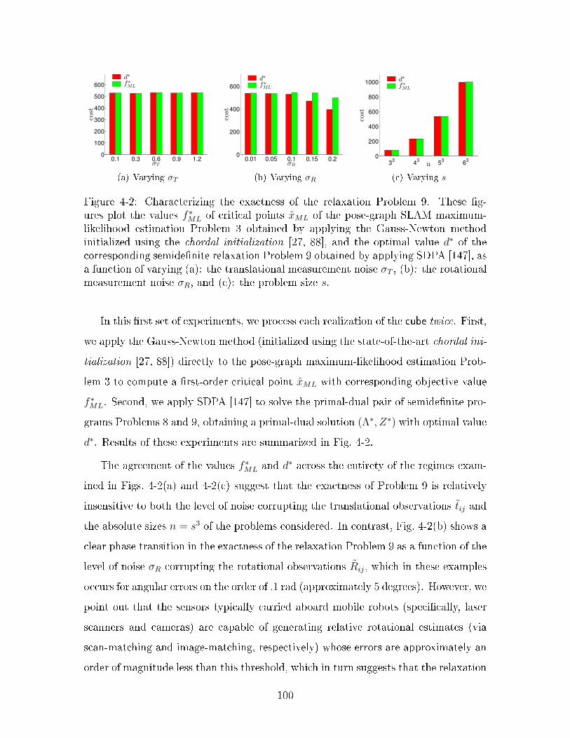
0.1 0.3 0.6 0.9 1.20
100
200
300
400
500
600
σT
cost
d⋆
f⋆ML
(a) Varying 𝜎𝑇
0.01 0.05 0.1 0.15 0.20
200
400
600
σR
cost
d⋆
f⋆ML
(b) Varying 𝜎𝑅
0
200
400
600
800
1000
n
cost
33
43
53
63
d⋆
f⋆ML
(c) Varying 𝑠
Figure 4-2: Characterizing the exactness of the relaxation Problem 9. These fig-ures plot the values 𝑓 *
𝑀𝐿 of critical points 𝑀𝐿 of the pose-graph SLAM maximum-likelihood estimation Problem 3 obtained by applying the Gauss-Newton methodinitialized using the chordal initialization [27, 88], and the optimal value 𝑑* of thecorresponding semidefinite relaxation Problem 9 obtained by applying SDPA [147], asa function of varying (a): the translational measurement noise 𝜎𝑇 , (b): the rotationalmeasurement noise 𝜎𝑅, and (c): the problem size 𝑠.
In this first set of experiments, we process each realization of the cube twice. First,
we apply the Gauss-Newton method (initialized using the state-of-the-art chordal ini-
tialization [27, 88]) directly to the pose-graph maximum-likelihood estimation Prob-
lem 3 to compute a first-order critical point 𝑀𝐿 with corresponding objective value
𝑓 *𝑀𝐿. Second, we apply SDPA [147] to solve the primal-dual pair of semidefinite pro-
grams Problems 8 and 9, obtaining a primal-dual solution (Λ*, 𝑍*) with optimal value
𝑑*. Results of these experiments are summarized in Fig. 4-2.
The agreement of the values 𝑓 *𝑀𝐿 and 𝑑* across the entirety of the regimes exam-
ined in Figs. 4-2(a) and 4-2(c) suggest that the exactness of Problem 9 is relatively
insensitive to both the level of noise corrupting the translational observations 𝑡𝑖𝑗 and
the absolute sizes 𝑛 = 𝑠3 of the problems considered. In contrast, Fig. 4-2(b) shows a
clear phase transition in the exactness of the relaxation Problem 9 as a function of the
level of noise 𝜎𝑅 corrupting the rotational observations 𝑖𝑗, which in these examples
occurs for angular errors on the order of .1 rad (approximately 5 degrees). However, we
point out that the sensors typically carried aboard mobile robots (specifically, laser
scanners and cameras) are capable of generating relative rotational estimates (via
scan-matching and image-matching, respectively) whose errors are approximately an
order of magnitude less than this threshold, which in turn suggests that the relaxation
100

GN-chordal GN-random
# nodes # measurements 𝑓() 𝜆min(𝐶()) 𝑓() 𝜆min(𝐶())sphere 2500 4949 1.0326 · 104 2.1458 · 10−5 7.2014 · 104 −5.1410 · 102sphere-a 2200 8647 7.8757 · 105 1.9597 · 10−4 1.0342 · 106 −8.5644 · 101torus 5000 9048 3.6542 · 104 1.0413 · 10−5 6.6950 · 105 −4.1791 · 102cube 8000 22236 1.2716 · 105 1.4208 · 10−4 1.2716 · 105 1.0658 · 10−4
garage 1661 6275 1.3150 · 102 1.8020 · 10−3 6.5748 · 104 −1.1136 · 102cubicle 5750 16869 1.6045 · 103 2.7418 · 10−5 8.7823 · 105 −8.1874 · 102rim 10195 29743 4.1819 · 104 1.6596 · 10−3 3.9560 · 105 −8.7068 · 102
Table 4.1: Results for large-scale pose-graph SLAM solution verification experiments
Problem 9 will remain exact under ordinary operating conditions.
4.4.2 Large-scale pose-graph SLAM datasets
The phenomenological simulation studies carried out in Section 4.4.1 suggest that the
relaxation Problem 9 should be exact under typical operating conditions for mobile
robots, and therefore the verification method based upon Theorem 6, which we refer
to as V2,6 should be able to correctly classify optimal versus suboptimal pose-graph
SLAM solutions, certifying the correctness of the former. In this next set of experi-
ments, we validate this hypothesis by applying V2 to several large-scale pose-graph
SLAM benchmark datasets.
Concretely, we consider two possible estimates = (𝑡, ) for each dataset: one
obtained by applying the Gauss-Newton method to Problem 6 using the state-of-the-
art chordal initialization (which we expect will often be the correct solution), and
the other obtained by applying the same Gauss-Newton method using a randomly-
sampled initialization (which we expect will typically produce a poor result). We
then apply the verification method V2 to each estimate in an attempt to certify
its optimality. Results from this experiment are summarized in Table 4.1, which
records the objective function value 𝑓() attained by each estimate, and the minimum
eigenvalue 𝜆min(𝐶()) of the corresponding certificate matrix 𝐶() defined in (4.26b).
We observe that in every one of our test cases, V2 succeeds in certifying the global
6We adopt this nomenclature in order to maintain consistency with that introduced in the orginalreport [26]; the method referred to therein as V1 was a precursor to the SE-Sync algorithm we developin the next chapter.
101

optimality of the estimate recovered by the Gauss-Newton method with chordal
initialization (note that 𝜆min(𝐶()) > 0 for each of these cases, and compare with
Theorem 6). In contrast, the suboptimal estimates recovered by the Gauss-Newton
method with random initialization have corresponding certificates 𝐶() with large
negative eigenvalues (note that this approach did in fact recover the globally optimal
solution for the cube dataset, despite its poor initialization). These results establish
that (i) the exactness of the relaxation Problem 9 does indeed hold under typical
operating conditions for mobile robots, as claimed, and (ii) as a result, V2 provides
an effective means of distinguishing correct from incorrect pose-graph SLAM solutions
in practice.
102

Chapter 5
Certifiably correct pose-graph SLAM
In the previous chapter, we showed that the semidefinite relaxation Problem 9 can
be exploited to produce a post hoc verification method for proving the correctness
of a given estimate ∈ SE(𝑑)𝑛 as a solution of the pose-graph SLAM maximum-
likelihood estimation Problem 3. Of course, this verification method only succeeds if
the supplied estimate actually is a correct solution for the SLAM inference problem.
Unfortunately, while existing graphical SLAM algorithms are often observed to work
well in many applications (as we saw, for example, in Section 4.4), it is precisely
their inability to guarantee the recovery of a correct solution that motivates this
thesis. This raises the question: How can we actually obtain such certifiably correct
solutions in practice?
In this chapter, we respond to the above question by developing an efficient pose-
graph SLAM inference algorithm that is capable of directly computing a globally
optimal solution for any instance of the pose-graph SLAM problem (4.3) whose so-
lutions could be successfully certified as optimal using V2. Recall that V2 attempts
to certify the optimality of a candidate solution ∈ SO(𝑑)𝑛 for the simplified pose-
graph SLAM problem (4.15) by showing that 𝑍 , T is optimal for the relaxation
Problem 9 (cf. Appendix D); consequently, V2 succeeds if and only if (i) the supplied
estimate actually is an optimal solution of Problem 6 and (ii) 𝑍 actually is an
The contents of this chapter are based upon material originally reported in [109].
103
optimal solution of Problem 9 (i.e., the relaxation is exact). Our approach is based
upon the recognition that if condition (ii) holds, then strictly speaking (i) is redun-
dant : rather than requiring that an optimal solution be supplied to V2, one can
instead simply recover from the optimal solution 𝑍 = T obtained by directly
solving the (convex) semidefinite relaxation Problem 9.
However, one complication impedes this approach: while it is true that Problem
9 can always be solved in polynomial time using interior-point methods [133, 140],
in practice the high computational cost of general-purpose semidefinite programming
algorithms prevents these methods1 from scaling effectively to problem instances in-
volving more than a few hundred poses [133]. Unfortunately, the pose-graphs encoun-
tered in real-world robotics applications are typically one to two orders of magnitude
larger than this maximum effective problem size, and are therefore well beyond the
reach of these general-purpose methods.
Consequently, the majority of our effort in this chapter will be devoted to the de-
velopment of a specialized optimization procedure that is capable of solving large-scale
instances of Problem 9 efficiently in practice. By combining this fast optimization
procedure with a simple rounding scheme, we obtain SE-Sync, a certifiably correct
pose-graph SLAM algorithm that is capable of efficiently recovering globally optimal
solutions of Problem 3 whenever exactness holds.
5.1 The SE-Sync algorithm
Our overall strategy in this chapter is to search for exact solutions of the (hard)
maximum-likelihood estimation Problem 3 by solving the (convex) semidefinite re-
laxation Problem 9. In order to realize this strategy as a practical algorithm, we
therefore require (i) a method that is able to solve Problem 9 effectively in appli-
cation, and (ii) a rounding procedure that recovers an optimal solution of Problem
3 from a solution of Problem 9 when exactness obtains, and a feasible approximate
1This encompasses the most commonly-used SDP software libraries, including SDPA [147], Se-DuMi [122], SDPT3 [134], and CSDP [11].
104

solution otherwise. In this section, we develop a pair of algorithms that fulfill these
requirements. Together, these procedures comprise SE-Sync, our proposed algorithm
for certifiably correct pose-graph SLAM.
5.1.1 Solving the semidefinite relaxation
In this section we develop a specialized optimization procedure for solving large-scale
instances of Problem 9 efficiently. To do so, we first exploit this problem’s low-rank,
geometric, and graphical structure to reduce it to an equivalent optimization problem
on a low-dimensional Riemannian manifold [10], and then design a fast Riemannian
optimization method to solve this reduction efficiently.
Simplifying Problem 9
Exploiting low-rank structure: The dominant computational cost when apply-
ing general-purpose semidefinite programming methods to solve Problem 9 is the need
to store and manipulate expressions involving the (large, dense) matrix variable 𝑍.
In particular, the 𝑂(𝑛3) computational cost of multiplying and factoring such expres-
sions quickly becomes intractable as the problem size 𝑛 increases. On the other hand,
in the typical case that exactness holds, we know that the actual solution 𝑍* of Prob-
lem 9 that we seek has a very concise description in the factored form 𝑍* = 𝑅*T𝑅* for
𝑅* ∈ SO(𝑑)𝑛. More generally, even in those cases where exactness fails, minimizers
𝑍* of Problem 9 generically have a rank 𝑟 not much greater than 𝑑, and therefore
admit a symmetric rank decomposition 𝑍* = 𝑌 *T𝑌 * for 𝑌 * ∈ R𝑟×𝑑𝑛 with 𝑟 ≪ 𝑑𝑛.
In a pair of papers, Burer and Monteiro [19, 20] proposed an elegant general
approach to exploit the fact that large-scale semidefinite programs often admit such
low-rank solutions: simply replace every instance of the decision variable 𝑍 with a
rank-𝑟 product of the form 𝑌 T𝑌 to produce a rank-restricted version of the original
problem. This substitution has the two-fold effect of (i) dramatically reducing the
size of the search space and (ii) rendering the positive semidefiniteness constraint
redundant, since 𝑌 T𝑌 ⪰ 0 for any choice of 𝑌 . The resulting rank-restricted form of
105

the problem is thus a low-dimensional nonlinear program, rather than a semidefinite
program. In the specific case of Problem 9, this produces:
Problem 10 (Rank-restricted semidefinite relaxation, NLP form).
𝑝*SDPLR = min𝑌 ∈R𝑟×𝑑𝑛
tr(𝑌 T𝑌 )
s.t. BlockDiag𝑑(𝑌T𝑌 ) = Diag(𝐼𝑑, . . . , 𝐼𝑑).
(5.1)
Provided that Problem 9 admits a solution 𝑍* with rank(𝑍*) ≤ 𝑟, we can recover
such a solution from an optimal solution 𝑌 * of Problem 10 according to 𝑍* = 𝑌 *T𝑌 *.
Exploiting geometric structure: In addition to exploiting Problem 9’s low-rank
structure, following Boumal [12] we also observe that the specific form of the con-
straints appearing in Problems 9 and 10 (i.e., that the 𝑑 × 𝑑 block-diagonals of 𝑍
and 𝑌 T𝑌 must be 𝐼𝑑) admits a nice geometric interpretation that can be exploited
to further simplify Problem 10. Introducing the block decomposition:
𝑌 ,(𝑌1 · · · 𝑌𝑛
)∈ R𝑟×𝑑𝑛, (5.2)
the block-diagonal constraints appearing in (5.1) are equivalent to:
𝑌 T𝑖 𝑌𝑖 = 𝐼𝑑, 𝑌𝑖 ∈ R𝑟×𝑑; (5.3)
i.e., they require that each 𝑌𝑖 be an element of the Stiefel manifold St(𝑑, 𝑟) (1.3).
Consequently, Problem 10 can be equivalently stated as an unconstrained Riemannian
optimization problem over a product of Stiefel manifolds:
Problem 11 (Rank-restricted semidefinite relaxation, Riemannian optimization form).
𝑝*SDPLR = min𝑌 ∈St(𝑑,𝑟)𝑛
tr(𝑌 T𝑌 ). (5.4)
This is the optimization problem that we will actually solve in practice.
106
Exploiting graphical structure: The reduction of Problem 9 to Problem 11 ob-
viates the need to form or manipulate the large, dense matrix variable 𝑍 directly.
However the data matrix that parameterizes each of Problems 6–11 is also dense
and of the same order as 𝑍, and so presents a similar computational difficulty. Here,
we develop an analogous concise description of by exploiting the structure of the
graph associated with the observation model (4.1).
Equations (4.15b) and (4.15c) provide a decomposition of in terms of the sparse
matrices 𝐿(𝜌), 𝑇 , and Ω, and the dense orthogonal projection matrix Π. However,
since Π is also a matrix derived from a sparse graph, we might suspect that it too
should admit some kind of sparse description. And indeed, it turns out that Π admits
a decomposition as:
¯𝐴() = 𝐿𝑄1 (5.5a)
Π = 𝐼𝑚 −¯𝐴()T𝐿−T𝐿−1
¯𝐴() (5.5b)
where equation (5.5a) is a thin LQ decomposition2 of the reduced incidence matrix
¯𝐴() of (this result is derived in Appendix B.2). Note that expression (5.5b)
for Π requires only the sparse lower-triangular factor 𝐿 from (5.5a), which can be
easily and efficiently obtained in practice (e.g. by applying successive Householder
transformations [48, Sec. 5.2.1] directly to¯𝐴() itself).
Together, equations (4.15b), (4.15c), and (5.5b) provide a concise description of
in terms of sparse matrices, as desired. We will exploit this decomposition in Section
5.1.1 to design a fast Riemannian optimization method for Problem 11.
The Riemannian Staircase
At this point, it is again instructive to compare Problem 11 with the simplified
maximum-likelihood estimation Problem 6 and its relaxation Problem 9. Since the
(special) orthogonal matrices satisfy condition (1.3) with 𝑘 = 𝑝 = 𝑑, we have the set
2This is the transpose of a QR decomposition [48, Sec. 5.2].
107

of inclusions:
SO(𝑑) ⊂ O(𝑑) = St(𝑑, 𝑑) ⊂ St(𝑑, 𝑑+ 1) ⊂ · · · ⊂ St(𝑑, 𝑟) ⊂ · · · (5.6)
and we can therefore view the set of rank-restricted Riemannian optimization prob-
lems (5.4) as comprising a hierarchy of relaxations of the maximum-likelihood estima-
tion (4.15) that are intermediate between Problem 7 and Problem 9 for 𝑑 < 𝑟 < 𝑑𝑛.
However, unlike Problem 9, the various instantiations of Problem 11 are nonconvex
due to the (re)introduction of the quadratic orthonormality constraints (1.3). It may
therefore not be clear whether anything has really been gained by relaxing Problem
6 to Problem 11, since it appears that we may have simply replaced one difficult non-
convex optimization problem with another. The following remarkable result (adapted
from Boumal et al. [15]) justifies this approach:
Proposition 7 (Global optima of Problem 11).
(i) If 𝑌 ∈ St(𝑑, 𝑟)𝑛 is a rank-deficient second-order critical point3 of Problem 11,
then 𝑌 is a global minimizer of Problem 11 and 𝑍* = 𝑌 T𝑌 is a solution of the
dual semidefinite relaxation Problem 9.
(ii) If 𝑟 ≥⌈√
𝑑(𝑑+ 1)𝑛⌉, then with probability 1 every first-order critical point of
Problem 11 is rank-deficient.4
Proof. Claim (i) is [15, Corollary 8], and claim (ii) is [15, Lemma 9] specialized to
Problem 11.
Proposition 7 immediately suggests an algorithm for obtaining solutions 𝑍* of
Problem 9 by applying a Riemannian optimization method to search successively
higher levels of the hierarchy of relaxations (5.4) until a rank-deficient second-order
critical point is obtained. This algorithm, the Riemannian Staircase [12, 15], is
summarized as Algorithm 5.1.
3That is, a point satisfying grad𝐹 (𝑌 ) = 0 and Hess𝐹 (𝑌 ) ⪰ 0 (cf. (5.7)–(5.10)).4The probability here refers to the distribution over the data matrix induced by the generative
model (4.1).
108

Algorithm 5.1 The Riemannian StaircaseInput: An initial point 𝑌 ∈ St(𝑑, 𝑟0)
𝑛, 𝑟0 ≥ 𝑑+ 1.Output: A minimizer 𝑌 * of Problem 11 corresponding to a solution 𝑍* = 𝑌 *T𝑌 * of
Problem 9.1: function RiemannianStaircase(𝑌 )2: for 𝑟 = 𝑟0, . . . , ⌈
√𝑑(𝑑+ 1)𝑛⌉ do
3: Starting at 𝑌 , apply a Riemannian optimization method5 to identify asecond-order
critical point 𝑌 * ∈ St(𝑑, 𝑟)𝑛 of Problem 11.4: if rank(𝑌 *) < 𝑟 then5: return 𝑌 *
6: else
7: Set 𝑌 ←(𝑌 *
01×𝑑𝑛
).
8: end if
9: end for
10: end function
We emphasize that while claim (ii) of Proposition 7 implies that we may have
to search up to 𝑂(√𝑛) levels of the hierarchy (5.4) in order to find a rank-deficient
second-order critical point, in practice this a gross overestimate; one or two “stairs”
in Algorithm 5.1 typically suffice.
A Riemannian optimization method for Problem 11
Proposition 7 and the Riemannian Staircase (Algorithm 5.1) provide a means of
obtaining global minimizers of Problem 9 by locally searching for second-order crit-
ical points of Problem 11. To that end, in this subsection we design a Riemannian
optimization method that will enable us to rapidly identify these critical points in
practice.
Equations (4.15b), (4.15c), and (5.5b) provide an efficient means of computing
products with by performing a sequence of sparse matrix multiplications and sparse
triangular solves (i.e., without the need to form directly). These operations are
sufficient to evaluate the objective appearing in Problem 11, as well as the corre-
sponding gradient and Hessian-vector products when considered as a function on the
5For example, the second-order Riemannian trust-region method [14, Algorithm 3].
109
ambient Euclidean space R𝑟×𝑑𝑛:
𝐹 (𝑌 ) , tr(𝑌 T𝑌 ) (5.7a)
∇𝐹 (𝑌 ) = 2𝑌 (5.7b)
∇2𝐹 (𝑌 )[ ] = 2 . (5.7c)
Furthermore, there are simple relations between the ambient Euclidean gradient and
Hessian-vector products in (5.7b) and (5.7c) and their corresponding Riemannian
counterparts when 𝐹 (·) is viewed as a function restricted to the embedded submani-
fold St(𝑑, 𝑟)𝑛 ⊂ R𝑟×𝑑𝑛. With reference to the orthogonal projection operator onto the
tangent space of St(𝑑, 𝑟)𝑛 at 𝑌 [38, eq. (2.3)]:
Proj𝑌 : 𝑇𝑌(R𝑟×𝑑𝑛
)→ 𝑇𝑌 (St(𝑑, 𝑟)𝑛)
Proj𝑌 (𝑋) = 𝑋 − 𝑌 SymBlockDiag𝑑(𝑌T𝑋)
(5.8)
the Riemannian gradient grad𝐹 (𝑌 ) is simply the orthogonal projection of the ambient
Euclidean gradient ∇𝐹 (𝑌 ) (cf. [3, eq. (3.37)]):
grad𝐹 (𝑌 ) = Proj𝑌 ∇𝐹 (𝑌 ). (5.9)
Similarly, the Riemannian Hessian-vector product Hess𝐹 (𝑌 )[ ] can be obtained as
the orthogonal projection of the ambient directional derivative of the gradient vector
field grad𝐹 (𝑌 ) in the direction of (cf. [3, eq. (5.15)]). A straightforward computa-
110

tion shows that this is given by:6
Hess𝐹 (𝑌 )[ ] = Proj𝑌
(D [grad𝐹 (𝑌 )] [ ]
)= Proj𝑌
(∇2𝐹 (𝑌 )[ ]− SymBlockDiag𝑑
(𝑌 T∇𝐹 (𝑌 )
)).
(5.10)
Equations (4.15b), (4.15c), and (5.5)–(5.10) provide an efficient means of com-
puting 𝐹 (𝑌 ), grad𝐹 (𝑌 ), and Hess𝐹 (𝑌 )[ ]. Consequently, we propose to employ a
truncated-Newton trust-region optimization method [36, 119] to solve Problem 11;
this approach will enable us to exploit the availability of an efficient routine for com-
puting Hessian-vector products Hess𝐹 (𝑌 )[ ] to implement a second-order optimiza-
tion method without the need to explicitly form or factor the dense matrix Hess𝐹 (𝑌 ),
and is therefore ideally suited for rapidly solving large-scale instances of Problem 11
to high precision [96, Sec. 7.1]. More specifically, we will apply the truncated-Newton
Riemannian Trust-Region (RTR) method [2, 14] to efficiently compute high-precision7
estimates of second-order critical points of Problem 11 in practice.
5.1.2 Rounding the solution
In the previous subsection, we described an efficient algorithmic approach for com-
puting minimizers 𝑌 * ∈ St(𝑑, 𝑟)𝑛 of Problem 11 that correspond to solutions 𝑍* =
𝑌 *T𝑌 * of Problem 9. However, our ultimate goal is to extract an optimal solution
𝑅* ∈ SO(𝑑)𝑛 of Problem 6 from 𝑍* whenever exactness holds, and a feasible ap-
proximate solution ∈ SO(𝑑)𝑛 otherwise. In this subsection, we develop a rounding
procedure satisfying these criteria. To begin, let us consider the (typical) case in
6We point out that equations (5.8), (5.9), and (5.10) correspond to equations (7), (8), and (9)in [12], with the caveat that [12]’s definition of 𝑌 is the transpose of ours. Our notation followsthe more common convention (cf. e.g. [38]) that elements of a Stiefel manifold are matrices withorthonormal columns, rather than rows.
7The requirement of high precision here is not superfluous: because Proposition 7(i) requires theidentification of rank-deficient second-order critical points, whatever local search technique we applyto Problem 11 must be capable of numerically approximating a critical point precisely enough thatits rank can be correctly determined.
111

which exactness obtains; here:
𝑌 *T𝑌 * = 𝑍* = 𝑅*T𝑅* (5.11)
for some optimal solution 𝑅* ∈ SO(𝑑)𝑛 of Problem 6. Since rank(𝑅*) = 𝑑, this implies
that rank(𝑌 *) = 𝑑 as well. Consequently, letting
𝑌 * = 𝑈𝑑𝛯𝑑𝑉T𝑑 (5.12)
denote a (rank-𝑑) thin singular value decomposition [48, Sec. 2.5.3] of 𝑌 *, and defining
𝑌 , 𝛯𝑑𝑉T𝑑 ∈ R𝑑×𝑑𝑛, (5.13)
it follows from substituting (5.12) into (5.11) that
𝑌 T𝑌 = 𝑍* = 𝑅*T𝑅*. (5.14)
Equation (5.14) implies that the 𝑑× 𝑑 block-diagonal of 𝑌 T𝑌 satisfies 𝑌 T𝑖 𝑌𝑖 = 𝐼𝑑 for
all 𝑖 ∈ [𝑛], i.e. 𝑌 ∈ O(𝑑)𝑛. Similarly, comparing the elements of the first block rows of
𝑌 T𝑌 and 𝑅*T𝑅* in (5.14) shows that 𝑌 T1 𝑌𝑗 = 𝑅*
1𝑅*𝑗 for all 𝑗 ∈ [𝑛]. Left-multiplying
this set of equalities by 𝑌1 and letting 𝐴 = 𝑌1𝑅*1 then gives:
𝑌 = 𝐴𝑅*, 𝐴 ∈ O(𝑑). (5.15)
Since any product of the form 𝐴𝑅* with 𝐴 ∈ SO(𝑑) is also an optimal solution of
Problem 6 (by gauge symmetry), equation (5.15) shows that 𝑌 as defined in (5.13)
is optimal provided that 𝑌 ∈ SO(𝑑) specifically. Furthermore, if this is not the
case, we can always make it so by left-multiplying 𝑌 by any orientation-reversing
element of O(𝑑), for example Diag(1, . . . , 1,−1). Thus, equations (5.12)–(5.15) give
a straightforward means of recovering an optimal solution of Problem 6 from 𝑌 *
whenever exactness holds.
Moreover, this procedure can be straightforwardly generalized to the case that
112

Algorithm 5.2 Rounding procedure for solutions of Problem 11Input: An optimal solution 𝑌 * ∈ St(𝑑, 𝑟)𝑛 of Problem 11.Output: A feasible point ∈ SO(𝑑)𝑛.1: function RoundSolution(𝑌 *)2: Compute a rank-𝑑 truncated singular value decomposition 𝑈𝑑𝛯𝑑𝑉
T𝑑 for 𝑌 *
and assign ← 𝛯𝑑𝑉T𝑑 .
3: Set 𝑁+ ← |𝑖 | det(𝑖) > 0|.4: if 𝑁+ < ⌈𝑛2 ⌉ then5: ← Diag(1, . . . , 1,−1).6: end if
7: for 𝑖 = 1, . . . , 𝑛 do8: Set 𝑖 ← NearestRotation(𝑖).9: end for
10: return 11: end function
exactness fails, thereby producing a convenient rounding scheme. Specifically, we can
consider the right-hand side of (5.13) as taken from a rank-𝑑 truncated singular value
decomposition of 𝑌 * (so that 𝑌 is an orthogonal transform of the best rank-𝑑 approx-
imation of 𝑌 *), multiply 𝑌 by an orientation-reversing element of O(𝑑) according to
whether a majority of its block elements have positive or negative determinant, and
then project each of 𝑌 ’s blocks to the nearest rotation matrix.8 This generalized
rounding scheme is formalized as Algorithm 5.2.
5.1.3 The complete algorithm
Combining the efficient optimization approach of Section 5.1.1 with the rounding
procedure of Section 5.1.2 produces SE-Sync (Algorithm 5.3), our proposed algorithm
for synchronization over the special Euclidean group.
When applied to an instance of SE(𝑑) synchronization, SE-Sync returns a feasible
point ∈ SE(𝑑)𝑛 for the maximum-likelihood estimation Problem 3 and the lower
bound 𝑝*SDP ≤ 𝑝*MLE for Problem 3’s optimal value. This lower bound provides an
upper bound on the suboptimality of any feasible point 𝑥 = (𝑡, 𝑅) ∈ SE(𝑑)𝑛 as a
8This is the special orthogonal Procrustes problem, which admits a simple solution based uponthe singular value decomposition (cf. e.g. [57, 137]).
113

Algorithm 5.3 The SE-Sync algorithmInput: An initial point 𝑌 ∈ St(𝑑, 𝑟0)
𝑛, 𝑟0 ≥ 𝑑+ 1.Output: A feasible estimate ∈ SE(𝑑)𝑛 for the maximum-likelihood estimation
Problem 3 and the lower bound 𝑝*SDP ≤ 𝑝*MLE for Problem 3’s optimal value.1: function SE-Sync(𝑌 )2: Set 𝑌 * ← RiemannianStaircase(𝑌 ). ◁ Solve Problems 9 & 113: Set 𝑝*SDP ← 𝐹 (𝑌 *T𝑌 *). ◁ 𝑍* = 𝑌 *T𝑌 *
4: Set ← RoundSolution(𝑌 *).5: Recover the optimal translational estimates 𝑡 corresponding to via (4.12),
using(1.9) and Lemma 8 in Appendix B.2 to evaluate the right-hand side efficiently.
6: Set ← (𝑡, ).7: return 𝑝*SDP, 8: end function
solution of Problem 3 according to:
𝐹 (𝑅T𝑅)− 𝑝*SDP ≥ 𝐹 (𝑅T𝑅)− 𝑝*MLE. (5.16)
Furthermore, in the (frequent) case that Problem 9 is exact, the estimate = (𝑡, ) ∈
SE(𝑑)𝑛 returned by Algorithm 5.3 attains this lower bound:
𝐹 (T) = 𝑝*SDP; (5.17)
verifying post hoc that (5.17) holds thus provides a means of computationally certifying
’s correctness as a solution of the maximum-likelihood estimation Problem 3. SE-
Sync is thus a certifiably correct algorithm for SE(𝑑) synchronization, as claimed.
5.2 Experimental results
In this section we evaluate SE-Sync’s performance on a variety of 3D pose-graph
SLAM datasets. Our experimental implementation of SE-Sync is written in MAT-
LAB, and takes advantage of the truncated-Newton RTR method supplied by the
Manopt toolbox [13]. For the purposes of the following experiments, we fix 𝑟 = 5 in
114
the Riemannian Staircase,9 and initialize RTR using a randomly sampled point on
St(3, 5)𝑛.
As a basis for comparison, we also evaluate the standard alternative approach of
applying the Gauss-Newton method [96] directly to Problem 3. We consider two vari-
ations of this approach: one using the common odometric initialization (“GN-odom”),
and another using the state-of-the-art chordal initialization (“GN-chord”) [27, 88]. Fi-
nally, since this chapter addresses the development of certifiably correct methods for
SE(𝑑) synchronization, and Gauss-Newton (unlike SE-Sync) does not natively pro-
vide solution certification, we also track the cost of applying the post hoc verification
method V2 described in Chapter 4 to certify the correctness of the estimates recovered
by the Gauss-Newton method with chordal initialization (“GN-chord-v2”).
5.2.1 Cube experiments
In this first set of experiments, we are interested in investigating how the performance
of SE-Sync is affected by factors such as problem size, measurement density, and
measurement noise level. To that end, we conduct a set of simulation studies that
enable us to interrogate each of these factors individually. Concretely, we consider
an ensemble of random realizations of the cube dataset; this scenario simulates a
robot traveling along a rectilinear path through a regular cubical lattice with a side
length of 𝑠, with an odometric measurement available between each pair of sequential
poses, and measurements between nearby nonsequential poses (loop closures) sampled
independently with probability 𝑝𝐿𝐶 . The measurement values themselves are obtained
by corrupting the true translation with additive mean-zero isotropic Gaussian noise
with standard deviation 𝜎𝑇 , and the true rotation with a multiplicative error obtained
by exponentiating an element of so(3) sampled from a mean-zero isotropic Gaussian
with standard deviation 𝜎𝑅. We fix default values for these parameters at 𝑠 = 10,
9This modification is purely for the sake of computational expedience: we have found empiricallythat ascending the hierarchy (5.4) to 𝑟 = 5 is sufficient to enable the recovery of a rank-deficientminimizer 𝑌 * of Problem 11 whenever exactness holds, and that when exactness fails, the roundedapproximate solutions obtained by ascending beyond this level are not appreciably better thanthose obtained by terminating here.
115

𝑝𝐿𝐶 = .1, 𝜎𝑇 = .5 m, and 𝜎𝑅 = .1 rad, and consider the effect of varying each of them
individually; our complete dataset consists of 30 realizations of the cube sampled from
the generative model just described for each joint setting of the parameters 𝑠, 𝑝𝐿𝐶 , 𝜎𝑇 ,
and 𝜎𝑅. Results for these experiments are shown in Fig. 5-1.
Overall, these results indicate that SE-Sync is capable of directly computing a
certifiably globally optimal solution in a running time that is comparable to (or in
these cases, even less than) that of a standard purely local search technique initialized
with a state-of-the-art method. Furthermore, this observation holds across a broad
range of operationally-relevant conditions. The one exception to this general rule
appears to be in the high-rotational-noise regime (Fig. 5-1(d)), where the exactness
of the relaxation Problem 9 breaks down and SE-Sync is unable to recover an exact
solution. Interestingly, the Gauss-Newton method with chordal initialization (GN-
chord) appears to perform remarkably well in this regime, although here it is no
longer possible to certify the correctness of its recovered estimates, as the certification
procedure V2 depends upon the same semidefinite relaxation as does SE-Sync.
5.2.2 Large-scale pose-graph SLAM datasets
In this next set of experiments, we evaluate SE-Sync’s performance on a standard suite
of large-scale SLAM benchmark datasets. We are interested in both the quality of
the estimates that SE-Sync obtains (in particular, whether the semidefinite relaxation
Problem 9 is exact for large-scale real-world examples like the garage and cubicle
datasets) and its computational cost when applied to these large problem instances.
As a basis for comparison, we also evaluate the performance of the Gauss-Newton
method with chordal initialization (GN-chord). Results for these experiments are
summarized in Table 5.1 and Fig. 5-2.
Overall, these results establish that SE-Sync provides an effective means of recov-
ering certifiably globally optimal solutions of large-scale pose-graph SLAM problems.
Furthermore (and consistent with our findings for the simulation studies in the previ-
ous subsection), the timing results reported in Table 5.1 indicate that the computa-
tional cost of computing these global minimizers using the Riemannian optimization
116

# nodes
3 3 5 3 7 3 9 3 11 3 13 3 15 3
Ob
jective
va
lue
0
2000
4000
6000
8000
10000
GN-odomGN-chordSE-Sync
# nodes
3 3 5 3 7 3 9 3 11 3 13 3 15 3
Co
mp
uta
tion
tim
e [
s]
0
10
20
30
40
50
60 GN-odomGN-chordGN-chord-v2SE-Sync
(a) Varying 𝑠 while holding 𝑝𝐿𝐶 = .1, 𝜎𝑇 = .5 m, 𝜎𝑅 = .1 rad.
pLC
0.2 0.4 0.6 0.8 1
Ob
jective v
alu
e
1000
2000
3000
4000
5000
6000
7000
8000
GN-odomGN-chordSE-Sync
pLC
0.2 0.4 0.6 0.8 1
Co
mp
uta
tio
n t
ime
[s]
0
10
20
30
40
50 GN-odomGN-chordGN-chord-v2SE-Sync
(b) Varying 𝑝𝐿𝐶 while holding 𝑠 = 10, 𝜎𝑇 = .5 m, 𝜎𝑅 = .1 rad.
σT
0.2 0.4 0.6 0.8 1 1.2
Ob
jective
va
lue
800
1000
1200
1400
1600
1800
2000
GN-odomGN-chordSE-Sync
σT
0.2 0.4 0.6 0.8 1 1.2
Com
pu
tatio
n tim
e [
s]
0
5
10
15
20
GN-odomGN-chordGN-chord-v2SE-Sync
(c) Varying 𝜎𝑇 while holding 𝑠 = 10, 𝑝𝐿𝐶 = .1, 𝜎𝑅 = .1 rad.
σR
0 0.05 0.1 0.15 0.2 0.25 0.3
Ob
jective
valu
e
800
1000
1200
1400
1600
1800
2000
2200
GN-odomGN-chordSE-Sync
σR
0.05 0.1 0.15 0.2 0.25 0.3
Com
puta
tion tim
e [s]
0
5
10
15
20
25 GN-odomGN-chordGN-chord-v2SE-Sync
(d) Varying 𝜎𝑅 while holding 𝑠 = 10, 𝑝𝐿𝐶 = .1, 𝜎𝑇 = .5 m.
Figure 5-1: Results for the cube experiments.
117

(a) sphere (b) torus (c) cube
(d) garage (e) cubicle (f) rim
Figure 5-2: Visualizations of the optimal solutions recovered by SE-Sync for thelarge-scale 3D pose-graph SLAM datasets listed in Table 5.1. Note that (a)–(c) aresynthetic, while (d)–(f) are real.
GN-chord SE-Sync# Nodes # Measurements Objective value Time [s] Objective value Time [s] Exact?
sphere 2500 4949 1.0326 · 104 48.12 1.0326 · 104 12.30 Xsphere-a 2200 8647 7.8759 · 105 60.38 7.8757 · 105 12.53 Xtorus 5000 9048 3.6544 · 104 58.20 3.6542 · 104 24.91 Xcube 8000 22236 1.2716 · 105 245.34 1.2716 · 105 84.74 Xgarage 1661 6275 1.3150 · 102 22.88 1.3150 · 102 200.00 Xcubicle 5750 16869 1.6045 · 103 159.92 1.6045 · 103 144.00 Xrim 10195 29743 4.1819 · 104 606.12 4.1819 · 104 426.01 X
Table 5.1: Results for the large-scale SLAM benchmarks.
118

scheme developed in Section 5.1.1 scales comparably with that of a fast local search
technique initialized with a state-of-the-art method.
119

120

Chapter 6
Conclusion
Robotics has the potential to make a tremendous positive impact on society over the
coming decades by increasing productivity, alleviating suffering, and preserving life.
At the same time, however, the widespread incorporation of robotics into the fabric of
everyday life, and especially in those safety-critical applications like transportation or
medicine where it can realize the greatest benefit, crucially depends upon autonomous
systems demonstrating that they can be trusted to function in a robust and reliable
way. This thesis contributes to that ultimate goal by developing a collection of algo-
rithms for solving the fundamental problem of simultaneous localization and mapping
that are capable of delivering certifiably correct performance.
6.1 Contributions
Concretely, the specific contributions of this thesis are:
1. We developed RISE, an incremental trust-region method for robust online sparse
least-squares estimation. RISE preserves the computational speed and super-
linear convergence rate of existing state-of-the-art online SLAM solvers while
providing superior robustness to nonlinearity and numerical ill-conditioning; in
particular, RISE is globally convergent under very mild hypotheses (namely,
that the objective is twice-continuously differentiable with bounded sublevel
121

sets). Consequently, RISE expands the class of SLAM problems that can be
reliably processed online to encompass essentially all reasonable inferential cost
functions.
2. We developed a post hoc solution verification method for computationally certi-
fying the correctness of recovered estimates for the archetypal problem of pose-
graph SLAM. This verification procedure enables the reliable use of existing
high-speed approximate inference methods (like RISE) by essentially equipping
these algorithms with a sense of introspection, enabling them to verify when
they have arrived at a correct solution, or conversely, to perform fault detec-
tion in those cases when recovered estimates fail to verify, possibly indicating a
failure in the underlying inference routine.
3. We developed SE-Sync, a pose-graph SLAM algorithm that is capable of effi-
ciently recovering certifiably globally optimal solutions across a broad spectrum
of operating conditions, including those typically encountered in practice. SE-
Sync preserves the speed and scalability of the Newton-type local optimization
methods that form the basis of existing state-of-the-art graphical SLAM algo-
rithms while enabling the computation of globally optimal estimates.
Collectively, these algorithms provide fast and robust inference and verification
methods for pose-graph SLAM in both the online and offline settings, and can be
straightforwardly incorporated into existing concurrent filtering and smoothing ar-
chitectures [146]. The result is a framework for real-time mapping and navigation
that preserves the computational speed of current state-of-the-art techniques while
delivering certifiably correct solutions.
6.2 Discussion and future research
This thesis was motivated by the need to develop reliable methods for solving a
fundamental perceptual problem arising in robotics; however, the majority of the
actual work contained herein directly addresses the design of efficient optimization
122

algorithms. The connection between our motivation and our methodology is provided
by the underlying assumption that the formulation of Problem 1 provides an adequate
encapsulation of the relevant engineering aspects of the SLAM problem, thus enabling
us to reduce the development of methods for its solution to an exercise in applied
mathematics. This has several implications for the scope of the methods developed
herein, as well as future research directions, which we briefly discuss.
First, while the algorithms developed in Chapters 4 and 5 of this thesis are ca-
pable of delivering certifiably correct solutions for the pose-graph SLAM estimation
Problem 3, the successful application of these algorithms, and the utility of the re-
sulting estimates so obtained, depend crucially upon the assumption that the prob-
abilistic generative model (4.1) underlying the maximum-likelihood estimation (4.3)
actually is a reasonable model of the true noise distribution corrupting the available
measurements 𝑖𝑗. While the distribution of sensor noise under nominal operating
conditions can often be characterized fairly well, and reasonably approximated using
(4.1) [61, 145], developing models that can allow for the possibility of exogeneous
sources of gross errors (such as false data associations) presents a serious challenge.
Some recent work has addressed this challenge by proposing “robustified” inference
schemes that attempt to attenuate the ill effects that occasional gross measurment
errors may have upon the recovered SLAM estimate [5, 76, 123, 124]. While these
approaches have indeed demonstrated some success in enhancing the resilience of
graphical SLAM algorithms to these disturbances, they too are ultimately heuristic
(as they all essentially reduce to the application of greedy strategies for deciding
which measurements to include in the estimation process), and it does not appear
that any of them strictly dominates the others in terms of performance [125]. It
would be interesting to see whether the convex relaxation approach developed in this
thesis could be generalized to perform joint measurement selection and parameter
estimation, in order to enable certifiably correct inference in the presence of grossly
contaminated observations; such a method would represent a significant advance over
current (heuristic) state-of-the-art approaches. We intend to pursue this investigation
in future work.
123

More generally, beyond the immediate algorithmic contributions outlined in the
preceding section, our hope is that this thesis can serve as a useful example of, and
tutorial introduction to, the power that the application of structure-exploiting convex
relaxation strategies can bring to bear on hard optimization problems arising in the
context of robotics. Certainly we are far from being the first to propose the use of
such strategies, but it seems that these techniques have not yet found widespread
application in robotic perception (in contrast to, for example, control). However,
the basic idea underlying these approaches is quite general (i.e. it is by no means
tightly-adjusted to the specifics of the SLAM problem considered herein), and it is
our hope that this thesis may therefore inspire others to consider the application of
these techniques in their own research.
124

Appendix A
Proof of Theorem 4
We prove Theorem 4 by means of Theorem 3. Since ℒ𝑆(𝑥(0)) is bounded, there exists
𝐷 > 0 such that ‖𝑥− 𝑥(0)‖ < 𝐷 for all 𝑥 ∈ ℒ𝑆(𝑥(0)). Define the convex open set
Ω = 𝑥 ∈ R𝑛 | ‖𝑥− 𝑥(0)‖ < 𝐷. (A.1)
Then Ω is a closed and bounded (hence compact) subset of R𝑛 containing the sub-
level set ℒ𝑆(𝑥(0)). Equation (3.11b) gives the elements of the Hessian matrix 𝜕2𝑆𝜕𝑥2 ,
which are continuous since 𝑟 ∈ 𝐶2, and therefore ‖𝜕2𝑆𝜕𝑥2 ‖ attains a maximum value 𝐿
on the compact set Ω; 𝐿 is thus a Lipschitz constant for ∇𝑆 on Ω. The same argu-
ment applied to the approximate Hessians 𝐵 whose elements are defined by equation
(3.12) shows that ‖𝐵‖ likewise attains a maximum 𝛽 on Ω. Finally, 𝑆 (as a sum-
of-squares function) is clearly lower-bounded by 0 everywhere. This establishes the
initial hypotheses of Theorem 3.
We now check each of the enumerated criteria (i)–(v) in turn. Condition (i) is
immediate from the definitions of the dog-leg and constrained Cauchy steps in and
(3.46) and (3.50). Condition (ii) is satisfied with 𝜁 = 0 since the gradients used in
Algorithm 3.4 are exact (cf. equation (3.13a)). Condition (iii) is satisfied using the
value of 𝛽 obtained in the preceding paragraph. Condition (iv) is trivially satisfied in
the case of the Cauchy step ℎ𝐶 , since this step is by definition always antiparallel to
the gradient (cf. equation (3.50)). In the case of the dog-leg step, we observe using
125

(3.44) that
‖ℎ𝑔𝑑‖ =
− ‖𝑔‖
2
𝑔𝑇𝐵𝑔𝑔
=‖𝑔‖3
𝑔𝑇𝐵𝑔≥ ‖𝑔‖
3
𝛽‖𝑔‖2=‖𝑔‖𝛽, (A.2)
so that (by virtue of the computation in Algorithm 3.3) ℎ𝑑𝑙 is also antiparallel to the
gradient whenever
∆(𝑖) <‖𝑔(𝑖)‖𝛽≤ ‖ℎ(𝑖)𝑔𝑑‖. (A.3)
Equation (A.3) will hold for all 𝑖 > 𝑁 for some sufficiently large 𝑁 by virtue of the
additional hypotheses (3.56) in effect for the purposes of this condition.
Finally, for condition (v), consider the predicted decrease for the Cauchy step
ℎ𝐶 = −𝜅𝑔 defined in (3.50) and (3.51):
pred(ℎ) = 𝜅‖𝑔‖2 − 1
2𝜅2𝑔𝑇𝐵𝑔. (A.4)
The full (i.e. unconstrained) Cauchy step has 𝜅 = ‖𝑔‖2𝑔𝑇𝐵𝑔
, in which case (A.4) becomes:
pred(ℎ) =
(‖𝑔‖2
𝑔𝑇𝐵𝑔
)‖𝑔‖2 − 1
2
(‖𝑔‖2
𝑔𝑇𝐵𝑔
)2
𝑔𝑇𝐵𝑔
=1
2· ‖𝑔‖
4
𝑔𝑇𝐵𝑔≥ ‖𝑔‖
2
2𝛽
(A.5)
since ‖𝐵‖ ≤ 𝛽. In the constrained case with 𝑔𝑇𝐵𝑔 > 0, 𝜅 = ∆/‖𝑔‖ only when
∆/‖𝑔‖ < ‖𝑔‖2/𝑔𝑇𝐵𝑔 (implying ∆𝑔𝑇𝐵𝑔 < ‖𝑔‖3), in which case (A.4) simplifies as
pred(ℎ) =
(∆
‖𝑔‖
)‖𝑔‖2 − 1
2
(∆
‖𝑔‖
)2
𝑔𝑇𝐵𝑔
= ∆‖𝑔‖ − 1
2
∆
‖𝑔‖2(∆𝑔𝑇𝐵𝑔
)≥ 1
2∆‖𝑔‖.
(A.6)
Finally, for the constrained case with 𝑔𝑇𝐵𝑔 ≤ 0, we observe that in fact 𝑔𝑇𝐵𝑔 = 0
since the Gauss-Newton Hessian approximation (3.13b) is always positive semidefi-
126

nite; thus 𝜅 = Δ‖𝑔‖ and (A.4) simplifies as
pred(ℎ) =
(∆
‖𝑔‖
)‖𝑔‖2 = ∆‖𝑔‖. (A.7)
Equations (A.5)–(A.7) show that the Cauchy step defined in (3.50) satisfies the uni-
form predicted decrease condition (3.59) with 𝑐 = 1 and 𝜎 = 𝛽. For the dog-leg step,
we simply observe that by virtue of (3.45), (3.46) and Lemma 2, pred(ℎ𝑑𝑙) ≥ pred(ℎ𝐶)
whenever ℎ𝑑𝑙 exists. This proves condition (v), and completes the proof.
127

128
Appendix B
The cycle space of a graph
In this section we briefly introduce the notion of the cycle space associated with a
graph; interested readers are directed to [8, 70] for additional detail.
B.1 Definition
Let = (𝒱 , ℰ) be a directed graph with 𝑛 = |𝒱| and 𝑚 = |ℰ | and F be a field. We
may associate to the free F-vector spaces 𝐶1(;F) and 𝐶0(;F) consisting of all
formal F-linear sums of ’s edges and vertices, respectively:
𝐶1(;F) ,
⎧⎨⎩∑𝑒∈ℰ
𝑐𝑒𝑒 | 𝑐𝑒 ∈ F
⎫⎬⎭ ∼= F𝑚, 𝐶0(;F) ,
∑𝑣∈𝒱
𝑐𝑣𝑣 | 𝑐𝑣 ∈ F
∼= F𝑛,
(B.1)
and define a corresponding boundary operator 𝜕1 : 𝐶1(;F)→ 𝐶0(;F) between them
as the unique linear extension of the assignment 𝜕1(𝑣, 𝑤) , 𝑤 − 𝑣 that maps each
directed edge (𝑣, 𝑤) ∈ ℰ to its (oriented) endpoints:
𝜕1 : 𝐶1(;F)→ 𝐶0(;F)
𝜕1
⎛⎝∑𝑒∈ℰ
𝑐𝑒𝑒
⎞⎠ =∑𝑣∈𝒱
⎛⎝ ∑𝑒∈𝛿+(𝑣)
𝑐𝑒 −∑
𝑒∈𝛿−(𝑣)
𝑐𝑒
⎞⎠ 𝑣.(B.2)
129

We denote the kernel of 𝜕1 by 𝑍(;F); it follows from (B.2) that this subspace is
given explicitly by:
𝑍(;F) , ker(𝜕1) =
⎧⎨⎩∑𝑒∈ℰ
𝑐𝑒𝑒 |∑
𝑒∈𝛿+(𝑣)
𝑐𝑒 =∑
𝑒∈𝛿−(𝑣)
𝑐𝑒 ∀𝑣 ∈ 𝒱
⎫⎬⎭ ⊆ 𝐶1(;F). (B.3)
If we interpret each edge 𝑒 = (𝑖, 𝑗) ∈ ℰ as the pathway for a flow from vertex 𝑖
to vertex 𝑗, and its associated coefficient 𝑐𝑒 ∈ F as the (directed) magnitude of that
flow, then the condition appearing in (B.3) is simply the requirement that the net
flows into and out of each vertex 𝑣 ∈ 𝒱 must be equal; we refer to this condition
as flow conservation, and (in consequence) to the elements 𝑧 ∈ 𝑍(;F) as flows or
(F-)cycles. The subspace 𝑍(;F) ⊆ 𝐶1(;F) itself is called the F-cycle space of .1
The support of a cycle in (B.3) is the set of edges 𝑒 ∈ ℰ with 𝑐𝑒 = 0. A cycle
is called simple if 𝑐𝑒 ∈ −1, 0, 1 for all 𝑒 ∈ ℰ , and a simple cycle is a circuit if its
support is weakly connected and for any 𝑣 ∈ 𝒱 there are at most two edges in the
support incident to 𝑣. An F-cycle basis is a set of circuits forming a basis for the
cycle space 𝑍(;F). It can be shown that dim(𝑍(;F)) = 𝑚 − 𝑛 + 𝑐, where 𝑐 is
the number of ’s weakly-connected components, and that 𝑍(;F) always admits a
cycle basis (cf. [70, Theorem 2.3]).2 Consequently, we let 𝜈 , 𝑚− 𝑛+ 𝑐, and refer to
this quantity as ’s cyclomatic number.
We can generalize this construction to an undirected graph 𝐺 by considering
the cycle space of one of its orientations . If and ′ are two orientations of
𝐺, then the cycle spaces 𝑍(;F) and 𝑍(′;F) are isomorphic under the mapping
𝜓 : 𝑍(;F)→ 𝑍(′;F) that reverses the sign of the scalars 𝑐𝑒 in (B.3) corresponding
to edges 𝑒 that are oriented differently in and ′. Consequently, the isomorphism
class of the cycle space 𝑍(;F) associated to 𝐺 in this way does not actually depend
upon the specific orientation selected (i.e. it is determined by the underlying graph
1Readers who are familiar with simplicial homology will also recognize 𝑍(;F) as 𝐻1(;F), thefirst homology group of considered as a simplicial 1-complex (hence the use of our highly suggestivechoice of notation in equations (B.1)–(B.3)).
2Note that this latter point is nontrivial: while the linear space 𝑍(;F) always admits a basis, acycle basis is a basis satisfying additional constraints.
130

𝐺 itself), and we are therefore justified in defining 𝑍(𝐺;F) , 𝑍(;F) and referring
to 𝑍(𝐺;F) as the cycle space of 𝐺.
The most common choices of the field F are F = Q and F = Z2 (the two-element
finite field); in these cases, the cycle spaces and bases are referred to as directed and
undirected, respectively.
B.2 Computing the orthogonal projection matrix
In this subsection we describe two methods for computing the matrix of the orthogonal
projection operator onto the directed cycle space of a weakly connected graph.
Let = (𝒱 , ℰ) be a weakly connected directed graph, F = R, and fix an ordering of
the edges ℰ and vertices 𝒱 (thus providing explicit identifications of 𝐶1() , 𝐶1(;R)
with R𝑚 and 𝐶0() , 𝐶0(;R) with R𝑛). Given any directed cycle basis 𝐵 =
𝐶1, . . . , 𝐶𝜈 ⊂ Z𝑚 for the directed cycle space 𝑍() , 𝑍(,R), we can construct
the associated cycle matrix Γ:
Γ ,(𝐶1 · · · 𝐶𝜈
)∈ Z𝑚×𝜈 . (B.4)
Since 𝐵 is a basis for 𝑍(), then image(Γ) = 𝑍(), and consequently the matrix Π
of the orthogonal projection operator 𝜋 : R𝑚 → 𝑍()) onto the directed cycle space
of is given by [90, eq. (5.13.12)]:
Π = ΓΓ†. (B.5)
Alternatively, we can also compute Π using the incidence matrix 𝐴(). Observe
that the matrix of the boundary operator 𝜕1 in (B.2) is actually 𝐴() itself; to see
this, simply note that the 𝑒th column of 𝐴() has a +1 in the row corresponding to
ℎ(𝑒), a −1 in the row corresponding to 𝑡(𝑒), and zeros elsewhere. Therefore, we also
have the alternative (although completely equivalent) characterization of 𝑍() as:
𝑍() = ker(𝐴()) ⊆ R𝑚. (B.6)
131

It follows from (B.6) that Π can also be expressed as (see again [90, eq. (5.13.12)]):
Π = 𝐼𝑚 − 𝐴()†𝐴(). (B.7)
While computing the pseudoinverse of a large matrix is in general an expensive
operation, in this case we can exploit the additional knowledge that 𝐴() is the
incidence matrix of a weakly-connected directed graph to speed up the computation
of the product on the right-hand side of (B.7). To do so, we will exploit the following
lemma:
Lemma 8. Let 𝐴 ∈ R𝑛×𝑚 be the incidence matrix for a weakly-connected directed
graph. Then the pseudoinverse of 𝐴 is given by:
𝐴† =¯𝐴T(¯𝐴
¯𝐴T)−1(𝐼𝑛−1 − 1
𝑛1𝑛−11
T𝑛−1 − 1
𝑛1𝑛−1
)(B.8)
where¯𝐴 ∈ R(𝑛−1)×𝑚 is the reduced incidence matrix obtained by removing the final
row of 𝐴.
Proof. By definition 𝐴 has a single instance of 1 and −1 in each of its columns, and
therefore 1T𝑛𝐴 = 0. We first show that 𝐴 can be decomposed as follows:
𝐴 =
⎛⎝ 𝐼𝑛−1
−1T𝑛−1
⎞⎠¯𝐴. (B.9)
Letting 𝑎 ∈ R1×𝑚 denote the final row of 𝐴, we observe that
1T𝑛𝐴 = 1
T𝑛
⎛⎝¯𝐴
𝑎
⎞⎠ = 1T𝑛−1¯
𝐴+ 𝑎 = 0; (B.10)
this implies that 𝑎 = −1T𝑛−1¯
𝐴, which is (B.9). Now let 𝐸 ,(𝐼𝑛−1 −1𝑛−1
)Tdenote
the matrix appearing in (B.9), and consider:
𝐴† = (𝐸¯𝐴)† =
¯𝐴†𝐸†. (B.11)
132

Since 𝐸 is full column rank, its pseudoinverse 𝐸† is
𝐸† =(𝐸T𝐸
)−1𝐸T; (B.12)
furthermore, observing that
(𝐸T𝐸
)−1=
⎛⎜⎝⎛⎝ 𝐼𝑛−1
−1T𝑛−1
⎞⎠T⎛⎝ 𝐼𝑛−1
−1T𝑛−1
⎞⎠⎞⎟⎠
−1
=(𝐼𝑛−1 + 1
T𝑛−11𝑛−1
)−1(B.13)
is the inverse of a rank-1 additive update of 𝐼𝑛−1, we may apply the Sherman-Morrison
formula [48, eq. (2.1.4)] to the right-hand side of (B.13) to compute:
(𝐸T𝐸
)−1= 𝐼𝑛−1 −
𝐼𝑛−11𝑛−11T𝑛−1𝐼𝑛−1
1 + 1T𝑛−1𝐼𝑛−11𝑛−1
= 𝐼𝑛−1 −1
𝑛1𝑛−11
T𝑛−1. (B.14)
Substituting (B.14) back into (B.12), we obtain:
(𝐸T𝐸)−1𝐸T =
(𝐼𝑛−1 −
1
𝑛1𝑛−11
T𝑛−1
)⎛⎝ 𝐼𝑛−1
−1T𝑛−1
⎞⎠T
=(𝐼𝑛−1 − 1
𝑛1𝑛−11
T𝑛−1 − 1
𝑛1𝑛−1
).
(B.15)
Similarly,¯𝐴 is full row rank (as it is the reduced incidence matrix of a weakly con-
nected graph), and therefore
¯𝐴† =
¯𝐴T(
¯𝐴
¯𝐴T)−1. (B.16)
Substituting (B.15) and (B.16) into (B.11) gives (B.8).
Applying Lemma 8 and the decomposition (B.9) for 𝐴(), the product on the
133
right-hand side of (B.7) can be expanded as:
𝐴()†𝐴() =
(¯𝐴()T
(¯𝐴()
¯𝐴()T
)−1 (𝐼𝑛−1 − 1
𝑛1𝑛−11
T𝑛−1 − 1
𝑛1𝑛−1
))⎛⎝⎛⎝ 𝐼𝑛−1
−1T𝑛−1
⎞⎠¯𝐴()
⎞⎠=
¯𝐴()T
(¯𝐴()
¯𝐴()T
)−1
¯𝐴().
(B.17)
Furthermore,¯𝐴() is full row rank, as it is the reduced incidence matrix of a weakly-
connected directed graph. Therefore, letting
¯𝐴() =
(𝐿 0
)𝑄 (B.18)
be an LQ decomposition3 of¯𝐴(), equation (B.17) is equivalent to:
𝐴()†𝐴() =¯𝐴()T𝐿−T𝐿−1
¯𝐴(). (B.19)
3This is the transpose of a QR decomposition [48, Sec. 5.2].
134

Appendix C
Simplifying the pose-graph estimation
problem
C.1 Deriving Problem 4 from Problem 3
In this section we show how to derive Problem 4 from Problem 3. Using the fact that
vec(𝑣) = 𝑣 for any 𝑣 ∈ R𝑑×1 and the fact that vec(𝑋𝑌 ) = (𝑌 𝑇 ⊗ 𝐼𝑘) vec(𝑋) for all
𝑋 ∈ R𝑚×𝑘 and 𝑌 ∈ R𝑘×𝑙 [59, Lemma 4.3.1], we can write each summand of (4.3) in
a vectorized form as:
𝜏𝑖𝑗𝑡𝑗 − 𝑡𝑖 −𝑅𝑖𝑡𝑖𝑗
22
= 𝜏𝑖𝑗𝑡𝑗 − 𝑡𝑖 −
(𝑡T𝑖𝑗 ⊗ 𝐼𝑑
)vec(𝑅𝑖)
22
=
(√𝜏𝑖𝑗𝐼𝑑)𝑡𝑗 − (
√𝜏𝑖𝑗𝐼𝑑)𝑡𝑖 −
√𝜏𝑖𝑗(𝑡T𝑖𝑗 ⊗ 𝐼𝑑
)vec(𝑅𝑖)
22
(C.1)
and
𝜅𝑖𝑗
𝑅𝑗 −𝑅𝑖𝑖𝑗
2𝐹
= 𝜅𝑖𝑗
vec(𝑅𝑗)− vec(𝑅𝑖𝑖𝑗)
22
=√
𝜅𝑖𝑗(𝐼𝑑 ⊗ 𝐼𝑑) vec(𝑅𝑗)−√𝜅𝑖𝑗
(T
𝑖𝑗 ⊗ 𝐼𝑑)
vec(𝑅𝑖)22.
(C.2)
135

Letting 𝑡 ∈ R𝑑𝑛 and 𝑅 ∈ R𝑑×𝑑𝑛 denote the concatenations of the 𝑡𝑖 and 𝑅𝑖 as defined
in (4.8), (C.1) and (C.2) imply that (4.3) can be rewritten in a vectorized form as:
𝑝*MLE = min𝑡∈R𝑑𝑛
𝑅∈SO(𝑑)𝑛
𝐵⎛⎝ 𝑡
vec(𝑅)
⎞⎠2
2
(C.3)
where the coefficient matrix 𝐵 ∈ R(𝑑+𝑑2)𝑚×(𝑑+𝑑2)𝑛 (with 𝑚 = |ℰ |) has the block
decomposition:
𝐵 ,
⎛⎝𝐵1 𝐵2
0 𝐵3
⎞⎠ (C.4)
and 𝐵1 ∈ R𝑑𝑚×𝑑𝑛, 𝐵2 ∈ R𝑑𝑚×𝑑2𝑛, and 𝐵3 ∈ R𝑑2𝑚×𝑑2𝑛 are block-structured matrices
whose block rows and columns are indexed by the elements of ℰ and 𝒱 , respectively,
and whose (𝑒, 𝑘)-block elements are given by:
(𝐵1)𝑒𝑘 =
⎧⎪⎪⎪⎪⎪⎨⎪⎪⎪⎪⎪⎩−√𝜏𝑘𝑗𝐼𝑑, 𝑒 = (𝑘, 𝑗) ∈ ℰ ,√𝜏𝑖𝑘𝐼𝑑, 𝑒 = (𝑖, 𝑘) ∈ ℰ ,
0𝑑×𝑑, otherwise,
(C.5a)
(𝐵2)𝑒𝑘 =
⎧⎪⎨⎪⎩−√𝜏𝑘𝑗(𝑡T𝑘𝑗 ⊗ 𝐼𝑑
), 𝑒 = (𝑘, 𝑗) ∈ ℰ ,
0𝑑×𝑑2 , otherwise,(C.5b)
(𝐵3)𝑒𝑘 =
⎧⎪⎪⎪⎪⎪⎨⎪⎪⎪⎪⎪⎩−√𝜅𝑘𝑗
(T
𝑘𝑗 ⊗ 𝐼𝑑), 𝑒 = (𝑘, 𝑗) ∈ ℰ ,
√𝜅𝑖𝑘(𝐼𝑑 ⊗ 𝐼𝑑), 𝑒 = (𝑖, 𝑘) ∈ ℰ ,
0𝑑×𝑑, otherwise.
(C.5c)
We can further expand the squared ℓ2-norm objective in (C.3) to obtain:
𝑝*MLE = min𝑡∈R𝑑𝑛
𝑅∈SO(𝑑)𝑛
⎛⎝ 𝑡
vec(𝑅)
⎞⎠T
𝐵T𝐵
⎛⎝ 𝑡
vec(𝑅)
⎞⎠ (C.6)
136

with
𝐵T𝐵 =
⎛⎝𝐵T1𝐵1 𝐵T
1𝐵2
𝐵T2𝐵1 𝐵T
2𝐵2 +𝐵T3𝐵3
⎞⎠ . (C.7)
We now derive explicit forms for each of the four distinct products on the right-hand
side of (C.7).
Case 𝐵T1𝐵1: Consider the (𝑖, 𝑗)-block of the product 𝐵T
1𝐵1:
(𝐵T1𝐵1)𝑖𝑗 =
∑𝑒∈ℰ
(𝐵1)T𝑒𝑖(𝐵1)𝑒𝑗. (C.8)
From (C.5a) we have that (𝐵1)𝑒𝑘 = 0 only if 𝑒 = (𝑖, 𝑘) or 𝑒 = (𝑘, 𝑗). Thus for 𝑖 = 𝑗,
(𝐵1)T𝑒𝑖(𝐵1)𝑒𝑗 = 0 only if 𝑒 = (𝑖, 𝑗) or 𝑒 = (𝑗, 𝑖), in which case (C.8) becomes:
(𝐵T1𝐵1)𝑖𝑗 = (±
√𝜏𝑒𝐼𝑑)
T(∓√𝜏𝑒𝐼𝑑) = −𝜏𝑒𝐼𝑑, 𝑖 = 𝑗. (C.9)
On the other hand, if 𝑖 = 𝑗, then (C.8) reduces to
(𝐵T1𝐵1)𝑖𝑖 =
∑𝑒∈ℰ|𝑒∈𝛿(𝑖)
(±√𝜏𝑒𝐼𝑑)
T(±√𝜏𝑒𝐼𝑑) =
∑𝑒∈ℰ|𝑒∈𝛿(𝑖)
𝜏𝑒𝐼𝑑. (C.10)
Comparing (C.9) and (C.10) with (4.4) shows that 𝐵T1𝐵1 = 𝐿(𝑊 𝜏 )⊗ 𝐼𝑑.
Case 𝐵T1𝐵2: Consider the (𝑖, 𝑗)-block of the product 𝐵T
1𝐵2:
(𝐵T1𝐵2)𝑖𝑗 =
∑𝑒∈ℰ
(𝐵1)T𝑒𝑖(𝐵2)𝑒𝑗. (C.11)
From (C.5b) we have that (𝐵2)𝑒𝑗 = 0 only if 𝑒 = (𝑗, 𝑘), and (C.5a) shows that
(𝐵1)T𝑒𝑖 = 0 only if 𝑒 = (𝑖, 𝑘) or 𝑒 = (𝑘, 𝑖). Thus for 𝑖 = 𝑗, (𝐵1)
T𝑒𝑖(𝐵2)𝑒𝑗 = 0 only if
𝑒 = (𝑗, 𝑖), in which case (C.11) becomes:
(𝐵T1𝐵2)𝑖𝑗 =
(√𝜏𝑗𝑖𝐼𝑑)
)T (−√𝜏𝑗𝑖 (𝑡T𝑗𝑖 ⊗ 𝐼𝑑)) = −𝜏𝑗𝑖((𝑡T𝑗𝑖 ⊗ 𝐼𝑑
), 𝑖 = 𝑗. (C.12)
137

On the other hand, for 𝑖 = 𝑗, (C.11) simplifies to:
(𝐵T1𝐵2)𝑗𝑗 =
∑(𝑗,𝑘)∈ℰ
(−√𝜏𝑗𝑘𝐼𝑑
)T (−√𝜏𝑗𝑘 (𝑡T𝑗𝑘 ⊗ 𝐼𝑑)) =∑
(𝑗,𝑘)∈ℰ
𝜏𝑗𝑘(𝑡T𝑗𝑘 ⊗ 𝐼𝑑
). (C.13)
Comparing (C.12) and (C.13) with (4.6) shows that 𝐵T1𝐵2 = 𝑉 ⊗ 𝐼𝑑.
Case 𝐵T2𝐵2: Consider the (𝑖, 𝑗)-block of the product 𝐵T
2𝐵2:
(𝐵T2𝐵2)𝑖𝑗 =
∑𝑒∈ℰ
(𝐵2)T𝑒𝑖(𝐵2)𝑒𝑗. (C.14)
Since (𝐵2)𝑒𝑖 = 0 unless 𝑒 = (𝑖, 𝑘) by (C.5b), (𝐵2)T𝑒𝑖(𝐵2)𝑒𝑗 = 0 only if 𝑖 = 𝑗. This
implies that (𝐵T2𝐵2)𝑖𝑗 = 0 for all 𝑖 = 𝑗, and
(𝐵T2𝐵2)𝑗𝑗 =
∑(𝑗,𝑘)∈ℰ
(−√𝜏𝑗𝑘
(𝑡𝑇𝑗𝑘 ⊗ 𝐼𝑑
))T (−√𝜏𝑗𝑘 (𝑡T𝑗𝑘 ⊗ 𝐼𝑑))=∑
(𝑗,𝑘)∈ℰ
𝜏𝑗𝑘(𝑡𝑗𝑘𝑡
T𝑗𝑘 ⊗ 𝐼𝑑
).
(C.15)
Comparing (C.15) with (4.7) then shows that 𝐵T2𝐵2 = Σ⊗ 𝐼𝑑.
Case 𝐵T3𝐵3: Finally, consider the (𝑖, 𝑗)-block of the product 𝐵T
3𝐵3:
(𝐵T3𝐵3)𝑖𝑗 =
∑𝑒∈ℰ
(𝐵3)T𝑒𝑖(𝐵3)𝑒𝑗. (C.16)
Using (C.5c), for 𝑖 = 𝑗 we find that
(𝐵3)T𝑒𝑖(𝐵3)𝑒𝑗 =
⎧⎪⎪⎪⎪⎪⎨⎪⎪⎪⎪⎪⎩
(−√𝜅𝑖𝑗
(𝑇
𝑖𝑗 ⊗ 𝐼𝑑))T (√
𝜅𝑖𝑗(𝐼𝑑 ⊗ 𝐼𝑑)), 𝑒 = (𝑖, 𝑗) ∈ ℰ ,(√
𝜅𝑗𝑖𝐼𝑑 ⊗ 𝐼𝑑)T (√
𝜅𝑗𝑖
(T
𝑗𝑖 ⊗ 𝐼𝑑))
, 𝑒 = (𝑗, 𝑖) ∈ ℰ ,
0𝑑2×𝑑2 , otherwise.
(C.17)
138

Consequently, for 𝑖 = 𝑗 (C.16) reduces to
(𝐵T3𝐵3)𝑖𝑗 =
⎧⎪⎪⎪⎪⎪⎨⎪⎪⎪⎪⎪⎩−𝜅𝑖𝑗(𝑖𝑗 ⊗ 𝐼𝑑), (𝑖, 𝑗) ∈ ℰ ,
−𝜅𝑗𝑖(T𝑗𝑖 ⊗ 𝐼𝑑), (𝑗, 𝑖) ∈ ℰ ,
0𝑑2×𝑑2 , otherwise.
(C.18)
Similarly, for 𝑖 = 𝑗 (C.5c) shows that
(𝐵3)T𝑒𝑖(𝐵3)𝑒𝑖 =
⎧⎪⎪⎪⎪⎪⎨⎪⎪⎪⎪⎪⎩
(−√𝜅𝑖𝑘
(𝑖𝑘 ⊗ 𝐼𝑑
))(−√𝜅𝑖𝑘
(T
𝑖𝑘 ⊗ 𝐼𝑑))
, (𝑖, 𝑘) ∈ ℰ ,(√𝜅𝑘𝑖(𝐼𝑑 ⊗ 𝐼𝑑)
) (√𝜅𝑘𝑖(𝐼𝑑 ⊗ 𝐼𝑑)
), (𝑘, 𝑖) ∈ ℰ ,
0𝑑2×𝑑2 , otherwise,
=
⎧⎪⎨⎪⎩𝜅𝑒(𝐼𝑑 ⊗ 𝐼𝑑), 𝑒 ∈ 𝛿(𝑖) ⊆ ℰ ,
0𝑑2×𝑑2 , otherwise,
(C.19)
and therefore
(𝐵T3𝐵3)𝑖𝑖 =
∑𝑒∈ℰ|𝑒∈𝛿(𝑖)
𝜅𝑒(𝐼𝑑 ⊗ 𝐼𝑑), (C.20)
Comparing (C.18) and (C.20) with (4.5) shows that 𝐵T3𝐵3 = 𝐿(𝜌)⊗ 𝐼𝑑.
Together, these results establish that 𝐵T𝐵 = 𝑀 ⊗ 𝐼𝑑, where 𝑀 is the matrix
defined in (4.9b), and consequently that Problem 3 is equivalent to Problem 4.
C.2 Deriving Problem 5 from Problem 4
In this subsection, we show how to analytically eliminate the translations 𝑡 appearing
in Problem 4 to obtain the simplified form of Problem 5. We make use of the following
lemma (cf. [16, Appendix A.5.5] and [46, Proposition 4.2]):
Lemma 9. Given 𝐴 ∈ Sym(𝑝) and 𝑏 ∈ R𝑝, the function
𝑓(𝑥) = 𝑥T𝐴𝑥+ 2𝑏T𝑥 (C.21)
139

attains a minimum if and only if 𝐴 ⪰ 0 and (𝐼𝑑 − 𝐴𝐴†)𝑏 = 0, in which case
min𝑥∈R𝑝
𝑓(𝑥) = −𝑏T𝐴†𝑏 (C.22)
and
argmin𝑥∈R𝑝
𝑓(𝑥) =
⎧⎨⎩−𝐴†𝑏+ 𝑈
⎛⎝0
𝑧
⎞⎠ | 𝑧 ∈ R𝑝−𝑟
⎫⎬⎭ , (C.23)
where 𝐴 = 𝑈Λ𝑈T is an eigendecomposition of 𝐴 and 𝑟 = rank(𝐴).
Now 𝐿(𝑊 𝜏 ) ⊗ 𝐼𝑑 ⪰ 0 since 𝐿(𝑊 𝜏 ) is a (necessarily positive semidefinite) graph
Laplacian, and 𝐼𝑑𝑛− (𝐿(𝑊 𝜏 )⊗𝐼𝑑)(𝐿(𝑊 𝜏 )⊗𝐼𝑑)† is the orthogonal projection operator
onto ker((𝐿(𝑊 𝜏 )⊗ 𝐼𝑑)T
)= ker(𝐿(𝑊 𝜏 ) ⊗ 𝐼𝑑) [90, eq. (5.13.12)]. Using the relation
vec(𝐴𝑌 𝐶) = (𝐶T ⊗ 𝐴) vec(𝑌 ) [59, Lemma 4.3.1], we find that 𝑦 ∈ ker(𝐿(𝑊 𝜏 ) ⊗ 𝐼𝑑)
if and only if 𝑦 = vec(𝑌 ) for some 𝑌 ∈ R𝑑×𝑛 satisfying 𝑌 𝐿(𝑊 𝜏 ) = 0, or equivalently
𝐿(𝑊 𝜏 )𝑌 T = 0. Since 𝐺 is connected, then ker(𝐿(𝑊 𝜏 )) = span1𝑛, and therefore
we must have 𝑌 T = 1𝑛𝑐T ∈ R𝑛×𝑑 for some 𝑐 ∈ R𝑑. Altogether, this establishes that:
ker(𝐿(𝑊 𝜏 )⊗ 𝐼𝑑) =
vec(𝑐1T
𝑛
)| 𝑐 ∈ R𝑑
. (C.24)
Now let 𝑏 = (𝑉 ⊗ 𝐼𝑑) vec(𝑅); we claim that 𝑏 ⊥ 𝑦 for all 𝑦 = vec(𝑌 ) ∈ ker(𝐿(𝑊 𝜏 )⊗
𝐼𝑑). To see this, observe that 𝑏 = vec(𝑅𝑉 T) and therefore ⟨𝑏, 𝑦⟩2 = ⟨𝑅𝑉 T, 𝑌 ⟩𝐹 =
tr(𝑌 𝑉 𝑅T). However, 1T𝑛𝑉 = 0 since the sum down each column of 𝑉 is identically 0
by (4.6), and therefore 𝑌 𝑉 = 0 by (C.24). This establishes that 𝑏 ⊥ ker(𝐿(𝑊 𝜏 )⊗ 𝐼𝑑)
for any value of 𝑅.
Consequently, if we fix 𝑅 ∈ SO(𝑑)𝑛 and consider performing the optimization
in (4.10) over the decision variables 𝑡 only, we can apply Lemma 9 to compute the
optimal value of the objective and a minimizing value 𝑡* of 𝑡 as functions of 𝑅. This
in turn enables us to analytically eliminate 𝑡 from (4.10), producing the equivalent
optimization problem:
𝑝*MLE = min𝑅∈SO(𝑑)
vec(𝑅)T((𝐿(𝜌) + Σ− 𝑉 T𝐿(𝑊 𝜏 )†𝑉
)⊗ 𝐼𝑑
)vec(𝑅), (C.25)
140

with a corresponding optimal translational estimate 𝑡* given by:
𝑡* = −(𝐿(𝑊 𝜏 )†𝑉 ⊗ 𝐼𝑑
)vec(𝑅*) (C.26)
Rewriting (C.25) and (C.26) in a more compact matricized form gives (4.11) and
(4.12), respectively.
C.3 Simplifying the translational data matrix 𝜏
In this subsection we derive the simplified form of the translational data matrix 𝜏
given in (4.15c) from the one originally presented in (4.11b). Our approach makes
frequent use of the incidence and reduced incidence matrices associated with a directed
graph. Consequently, we begin by developing a collection of lemmas characterizing
several properties of these objects.
Lemma 10. Let 𝐴 ∈ R𝑛×𝑚 and¯𝐴 ∈ R(𝑛−1)×𝑚 be the incidence and reduced incidence
matrices of a weakly-connected directed graph and 𝑆 ∈ Sym(𝑚) positive definite. Then
𝑆12𝐴T
(𝐴𝑆𝐴T
)†𝐴𝑆
12 = 𝑆
12
¯𝐴T(¯𝐴𝑆
¯𝐴T)−1
¯𝐴𝑆
12 . (C.27)
Proof. The proof proceeds via straightforward computation:
𝑆12𝐴T
(𝐴𝑆𝐴T
)†𝐴𝑆
12 = 𝑆
12𝐴T(𝐴†)T𝑆−1𝐴†𝐴𝑆
12
= 𝑆12𝐴T
⎛⎝⎛⎝𝐼𝑛−1 − 1𝑛1𝑛−11
T𝑛−1
− 1𝑛1T𝑛−1
⎞⎠ (¯𝐴
¯𝐴T)−1
¯𝐴
⎞⎠𝑆−1(
¯𝐴T(¯𝐴
¯𝐴T)−1(𝐼𝑛−1 − 1
𝑛1𝑛−11
T𝑛−1 − 1
𝑛1𝑛−1
))𝐴𝑆
12
= 𝑆12𝐴T
⎛⎝𝐼𝑛−1 − 1𝑛1𝑛−11
T𝑛−1
− 1𝑛1T𝑛−1
⎞⎠(¯𝐴†)T 𝑆−1
¯𝐴†
(𝑎)⏞ ⏟ (𝐼𝑛−1 − 1
𝑛1𝑛−11
T𝑛−1 − 1
𝑛1𝑛−1
)𝐴𝑆
12 ,
(C.28)
where we have applied Lemma 8 in passing from line 1 to line 2 of (C.28) and equation
(B.16) in passing from line 2 to line 3. Now we use the decomposition (B.9) and
141

develop the term labeled (a) in (C.28) as follows:
(𝐼𝑛−1 − 1
𝑛1𝑛−11
T𝑛−1 − 1
𝑛1𝑛−1
)𝐴 =
(𝐼𝑛−1 − 1
𝑛1𝑛−11
T𝑛−1 − 1
𝑛1𝑛−1
)⎛⎝ 𝐼𝑛−1
−1T𝑛−1
⎞⎠¯𝐴
= (𝐼𝑛−1 −1
𝑛1𝑛−11
T𝑛−1 +
1
𝑛1𝑛−11
T𝑛−1)¯
𝐴
=¯𝐴.
(C.29)
Substituting (C.29) into (C.28), we obtain
𝑆12𝐴T
(𝐴𝑆𝐴T
)†𝐴𝑆
12 = 𝑆
12
¯𝐴T(¯𝐴†)T 𝑆−1
¯𝐴†
¯𝐴𝑆
12
= 𝑆12
¯𝐴T(¯𝐴𝑆
¯𝐴T)†
¯𝐴𝑆
12
= 𝑆12
¯𝐴T(¯𝐴𝑆
¯𝐴T)−1
¯𝐴𝑆
12
(C.30)
since¯𝐴𝑆
¯𝐴T is invertible as
¯𝐴 has full row rank.
Lemma 11 (Lemma 22 in [23]). Let¯𝐴 ∈ R(𝑛−1)×𝑚 be the reduced incidence matrix
of a weakly-connected directed graph and 𝑆 ∈ Sym(𝑚) positive definite. Then
𝐼𝑚 − 𝑆12
¯𝐴T(¯𝐴𝑆
¯𝐴T)−1
¯𝐴𝑆
12 = 𝑆− 1
2 Γ(ΓT𝑆−1Γ
)−1ΓT𝑆− 1
2 (C.31)
where Γ ∈ Z𝑚×(𝑚−𝑛+1) is the cycle matrix of a directed cycle basis of .
With the aid of Lemmas 8–11, we now derive (4.15c) from (4.11b). To begin, we
recall from Appendix C.1 that
𝜏 ⊗ 𝐼𝑑 =(
Σ− 𝑉 T𝐿(𝑊 𝜏 )†𝑉)⊗ 𝐼𝑑
= 𝐵T2𝐵2 −𝐵T
2𝐵1
(𝐵T
1𝐵1
)†𝐵T
1𝐵2
= 𝐵T2
(𝐼𝑑𝑚 −𝐵1
(𝐵T
1𝐵1
)†𝐵T
1
)𝐵2,
(C.32)
where 𝐵1 and 𝐵2 are the matrices defined in (C.5a) and (C.5b), respectively. With
the aid of Ω and 𝑇 as defined in (4.13) and (4.14), respectively, we may write 𝐵1 and
142
𝐵2 alternatively as:
𝐵1 = Ω12𝐴T ⊗ 𝐼𝑑, 𝐵2 = Ω
12𝑇 ⊗ 𝐼𝑑, (C.33)
where 𝐴 , 𝐴() is the incidence matrix of . Substituting (C.33) into (C.32), we
derive:
𝜏 ⊗ 𝐼𝑑 = 𝐵T2
(𝐼𝑑𝑚 −𝐵1(𝐵
T1𝐵1)
†𝐵T1
)𝐵2
= 𝐵T2
(𝐼𝑑𝑚 −
(Ω
12𝐴T ⊗ 𝐼𝑑
)((Ω
12𝐴T ⊗ 𝐼𝑑
)T (Ω
12𝐴T ⊗ 𝐼𝑑
))† (Ω
12𝐴T ⊗ 𝐼𝑑
)T)𝐵2
= 𝐵T2
(𝐼𝑑𝑚 −
(Ω
12𝐴T ⊗ 𝐼𝑑
)((𝐴Ω𝐴T
)† ⊗ 𝐼𝑑)(Ω12𝐴T ⊗ 𝐼𝑑
)T)𝐵2
= 𝐵T2
(𝐼𝑑𝑚 −
(Ω
12𝐴T
(𝐴Ω𝐴T
)†𝐴Ω
12
)⊗ 𝐼𝑑)
)𝐵2
= 𝐵T2
[(𝐼𝑚 − Ω
12𝐴T
(𝐴Ω𝐴T
)†𝐴Ω
12
)⊗ 𝐼𝑑
]𝐵2
=
(𝑇TΩ
12
(𝐼𝑚 − Ω
12𝐴T
(𝐴Ω𝐴T
)†𝐴Ω
12
)TΩ
12𝑇
)⊗ 𝐼𝑑.
(C.34)
Applying Lemma 10 to the final line of (C.34), we find:
𝜏 ⊗ 𝐼𝑑 =
(𝑇TΩ
12
(𝐼𝑚 − Ω
12
¯𝐴T(¯𝐴Ω
¯𝐴T)−1
¯𝐴Ω
12
)TΩ
12𝑇
)⊗ 𝐼𝑑, (C.35)
where¯𝐴 ,
¯𝐴() is the reduced incidence matrix of . Applying Lemma 11 to (C.35)
produces:
𝜏 ⊗ 𝐼𝑑 =(𝑇TΩ
12
(Ω− 1
2 Γ(ΓTΩ−1Γ
)−1ΓTΩ− 1
2
)Ω
12𝑇T
)⊗ 𝐼𝑑, (C.36)
or equivalently:
𝜏 = 𝑇TΓ(ΓTΩ−1Γ
)−1ΓT𝑇. (C.37)
Finally, we observe that
Γ(ΓTΩ−1Γ
)−1ΓT = Γ
(ΓTΩ−1Γ
)†ΓT = (ΓΓ†)Ω
(ΓΓ†)T = ΠΩΠ (C.38)
143

since Π = ΓΓ† by (B.5) and Π = ΠT since Π is an orthogonal projection operator.
Substituting (C.38) into (C.37) gives (4.15c).
C.4 Deriving Problem 9 from Problem 8
This derivation is a straightforward application of the well-known duality theory for
semidefinite programs [140]. Letting 𝜆𝑖𝑢𝑣 ∈ R denote the (𝑢, 𝑣)-element of the 𝑖th
diagonal block of Λ for 𝑖 = 1, . . . , 𝑛 and 𝑢, 𝑣 ∈ [𝑑] with 𝑢 ≤ 𝑣, we can rewrite Problem
8 in the primal standard form of [140, eq. (1)] as:
−𝑝*SDP = min𝜆∈R
𝑑(𝑑+1)2 𝑛
𝑐𝑇𝜆
s.t. 𝐹 (𝜆) ⪰ 0,
(C.39)
with the problem data in (C.39) given explicitly by:
𝐹 (𝜆) , 𝐹0 +𝑛∑
𝑖=1
∑𝑢,𝑣
𝜆𝑖𝑢𝑣𝐹𝑖𝑢𝑣,
𝐹0 = 𝑄,
𝐹𝑖𝑢𝑣 =
⎧⎪⎨⎪⎩−Diag(𝑒𝑖)⊗ 𝐸𝑢𝑢, 𝑢 = 𝑣,
−Diag(𝑒𝑖)⊗ (𝐸𝑢𝑣 + 𝐸𝑣𝑢), 𝑢 = 𝑣,
𝑐𝑖𝑢𝑣 =
⎧⎪⎨⎪⎩−1, 𝑢 = 𝑣,
0, 𝑢 = 𝑣.
(C.40)
The standard dual problem for (C.39) is then (cf. equations (1) and (27) of [140]):
−𝑑 = max𝑍∈Sym(𝑑𝑛)
− tr(𝐹0𝑍)
s.t. tr (𝐹𝑖𝑢𝑣𝑍) = 𝑐𝑖𝑢𝑣 ∀𝑖 ∈ [𝑛], 𝑢, 𝑣 ∈ [𝑑], 𝑢 ≤ 𝑣,
𝑍 ⪰ 0.
(C.41)
144

Comparing (C.41) with (C.40) reveals that the equality constraints are satisfied pre-
cisely when 𝑍’s (𝑑× 𝑑)-block-diagonal is comprised of identity matrices, which gives
the form of Problem 9. Furthermore, since − Λ ≻ 0 for any Λ = −𝑠𝐼𝑑𝑛 with
𝑠 > ‖‖2 is strictly feasible for Problem 8 (hence also (C.39)) and 𝐼𝑑𝑛 ≻ 0 is strictly
feasible for (C.41), Theorem 3.1 of [140] implies that the optimal sets of (C.39) and
(C.41) are nonempty, and that strict duality holds between them (so that the optimal
value of Problem 9 is 𝑝*SDP, as claimed).
145

146
Appendix D
Proof of Theorem 6
In this appendix, we provide a proof of Theorem 6. In brief, our approach is based
upon the observation that since Problem 8 is obtained from Problem 6 via Lagrangian
relaxation, the Lagrange multipliers Λ(𝑅*) associated with an optimal solution 𝑅* ∈
SO(𝑑)𝑛 of the extrinsic (i.e. constrained) formulation of Problem 6 provide an optimal
solution of Problem 8 whenever exactness holds; in turn, this optimal solution Λ(𝑅*)
provides a KKT certificate of 𝑍* = 𝑅*T𝑅* as a solution of Problem 9. Theorem 5
then implies that 𝑅* is a globally optimal solution of Problem 6.
We begin by showing that Λ(𝑅) as defined in (4.26a) is indeed the correct expres-
sion for the Lagrange multiplier matrix (note that (D.1) is the first-order necessary
condition for the Lagrangian (4.19)):
Lemma 12. Let 𝑅 ∈ SO(𝑑)𝑛 be a first-order critical point of Problem 6. Then
(− Λ(𝑅)
)𝑅T = 0, (D.1)
where Λ(𝑅) is as defined in (4.26a).
Proof. The proof is a straightforward application of a simple relation between the
gradient ∇𝐹 (𝑅) of the function 𝐹 (𝑅) , tr(𝑅T𝑅) considered as a function on the
ambient Euclidean space R𝑑×𝑑𝑛 and the Riemannian gradient grad𝐹 (𝑅) of 𝐹 con-
sidered as a function on the embedded Riemannian submanifold SO(𝑑)𝑛 ⊂ R𝑑×𝑑𝑛.
147

Specifically,
grad𝐹 (𝑅) = Proj𝑅∇𝐹 (𝑅), (D.2)
where Proj𝑅 : 𝑇𝑅(R𝑑×𝑑𝑛)→ 𝑇𝑅(SO(𝑑)𝑛) gives the orthogonal projection operator onto
the tangent space of SO(𝑑)𝑛 at 𝑅 [3, eq. (3.37)]; this latter is given explicitly by:
Proj𝑅 : 𝑇𝑅(R𝑑×𝑑𝑛
)→ 𝑇𝑅 (SO(𝑑)𝑛)
Proj𝑅(𝑋) = 𝑋 −𝑅 SymBlockDiag𝑑(𝑅T𝑋).
(D.3)
Straightforward differentiation shows that ∇𝐹 (𝑅) = 2𝑅, and grad𝐹 (𝑅) = 0 since
𝑅 is a first-order critical point of Problem 6 by hypothesis; equations (D.2) and (D.3)
therefore imply that
0 = 2𝑅− 2𝑅 SymBlockDiag𝑑(𝑅T𝑅). (D.4)
Dividing both sides of (D.4) by 2 and taking the transpose produces (D.1), using the
definition of Λ(𝑅) given in (4.26a).
We now prove Theorem 6 with the aid of Lemma 12.
Proof of Theorem 6. Our approach is to show that the hypotheses of Theorem 6 imply
that 𝑍 , 𝑅T𝑅 is an optimal solution of Problem 9. To that end, recall that since
Problems 8 and 9 satisfy strong duality (cf. Section C.4), 𝑍 is an optimal solution of
Problem 9 if and only if there exists a Λ ∈ SBD(𝑑, 𝑛) such that:
1. − Λ ⪰ 0 (feasibility);
2. (− Λ)𝑍 = 0 (complementary slackness).
With Λ = Λ(𝑅) as defined in (4.26a), condition 1 above is exactly the hypothesis
that 𝐶(𝑅) ⪰ 0, and condition 2 follows from Lemma 12 and the hypothesis that 𝑅 is
a first-order critical point of Problem 6, since
(− Λ(𝑅))𝑍 = (− Λ(𝑅))(𝑅T𝑅
)= 0. (D.5)
148

This establishes that 𝑍 = 𝑅T𝑅 is an optimal solution of Problem 9. The optimality
of 𝑅 as a solution of Problem 6 then follows from Theorem 5.
149

150

Bibliography
[1] K.J. Åström and R.M. Murray. Feedback Systems: An Introduction for Scien-tists and Engineers. Princeton University Press, Princeton, NJ, USA, 2008.
[2] P.-A. Absil, C.G. Baker, and K.A. Gallivan. Trust-region methods on Rieman-nian manifolds. Found. Comput. Math., 7(3):303–330, July 2007.
[3] P.-A. Absil, R. Mahony, and R. Sepulchre. Optimization Algorithms on MatrixManifolds. Princeton University Press, 2008.
[4] P. Agarwal, W. Burgard, and C. Stachniss. Survey of geodetic mapping meth-ods: Geodetic approaches to mapping and the relationship to graph-based slam.IEEE Robotics & Automation Magazine, 21(3):63–80, September 2014.
[5] P. Agarwal, G.D. Tipaldi, L. Spinello, C. Stachniss, and W. Burgard. Dynamiccovariance scaling for robust map optimization. In IEEE Intl. Conf. on Roboticsand Automation (ICRA), Hong Kong, China, June 2014.
[6] T. Bailey, J. Nieto, J. Guivant, M. Stevens, and E. Nebot. Consistency ofthe EKF-SLAM algorithm. In IEEE/RSJ Intl. Conf. on Intelligent Robots andSystems (IROS), pages 3562–3568, Beijing, China, October 2006.
[7] A.S. Bandeira, N. Boumal, and A. Singer. Tightness of the maximum like-lihood semidefinite relaxation for angular synchronization. arXiv preprintarXiv:1411.3272v2, 2015.
[8] N. Biggs. Algebraic potential theory on graphs. Bull. London Math. Soc., 29:641–682, 1997.
[9] C.M. Bishop. Pattern Recognition and Machine Learning. Springer Sci-ence+Business Media, New York, 2006.
[10] W.M. Boothby. An Introduction to Differentiable Manifolds and RiemannianGeometry. Academic Press, London, 2nd edition, 2003.
[11] B. Borchers. CSDP, a C library for semidefinite programming. OptimizationMethods and Software, 11(1–4):613–623, 1999.
[12] N. Boumal. A Riemannian low-rank method for optimization over semidefinitematrices with block-diagonal constraints. arXiv preprint: arXiv:1506.00575v2,2015.
151

[13] N. Boumal, B. Mishra, P.-A. Absil, and R. Sepulchre. Manopt, a MATLABtoolbox for optimization on manifolds. Journal of Machine Learning Research,15(1):1455–1459, 2014.
[14] N. Boumal, P.-A. Absil, and C. Cartis. Global rates of convergence for noncon-vex optimization on manifolds. arXiv preprint: arXiv:1605.08101v1, 2016.
[15] N. Boumal, V. Voroninski, and A.S. Bandeira. The non-convex Burer-Monteiro approach works on smooth semidefinite programs. arXiv preprintarXiv:1606.04970v1, June 2016.
[16] S. Boyd and L. Vandenberghe. Convex Optimization. Cambridge UniversityPress, 2004.
[17] D.C. Brown. A solution to the general problem of multiple station analyticalstereotriangulation. Technical Report AFMTC TR 58-8, Patrick Air Force Base,FL, USA, 1958.
[18] D.C. Brown. The bundle adjustment – progress and prospects. Int. ArchivesPhotogrammetry, 21(3), 1976.
[19] S. Burer and R.D.C. Monteiro. A nonlinear programming algorithm for solvingsemidefinite programs via low-rank factorization. Math. Program., 95:329–357,2003.
[20] S. Burer and R.D.C. Monteiro. Local minima and convergence in low-ranksemidefinite programming. Math. Program., 103:427–444, 2005.
[21] D. Burschka, J.J. Corso, M. Dewan, W. Lau, M. Li, H. Lin, P. Marayong,N. Ramey, G.D. Hager, B. Hoffman, D. Larkin, and C. Hasser. Navigating innerspace: 3-D assistance for minimally invasive surgery. Robotics and AutonomousSystems, 52(1):5–26, 2005.
[22] C. Cadena, L. Carlone, H. Carrillo, Y. Latif, D. Scaramuzza, J. Neira, I.D.Reid, and J.J. Leonard. Past, present, and future of simultaneous local-ization and mapping: Towards the robust-perception age. arXiv preprintarXiv:1606.05830v2, 2016.
[23] L. Carlone and A. Censi. From angular manifolds to the integer lattice: Guaran-teed orientation estimation with application to pose graph optimization. IEEETrans. Robotics, 30(2):475–492, April 2014.
[24] L. Carlone and F. Dellaert. Duality-based verification techniques for 2D SLAM.In IEEE Intl. Conf. on Robotics and Automation (ICRA), pages 4589–4596,Seattle, WA, May 2015.
[25] L. Carlone, R. Aragues, J. Castellanos, and B. Bona. A fast and accurateapproximation for planar pose graph optimization. Intl. J. of Robotics Research,33(7):965–987, 2014.
152

[26] L. Carlone, D.M. Rosen, G. Calafiore, J.J. Leonard, and F. Dellaert. La-grangian duality in 3D SLAM: Verification techniques and optimal solutions.In IEEE/RSJ Intl. Conf. on Intelligent Robots and Systems (IROS), Hamburg,Germany, September 2015.
[27] L. Carlone, R. Tron, K. Daniilidis, and F. Dellaert. Initialization techniquesfor 3D SLAM: A survey on rotation estimation and its use in pose graph op-timization. In IEEE Intl. Conf. on Robotics and Automation (ICRA), pages4597–4605, Seattle, WA, May 2015.
[28] R.G. Carter. On the global convergence of trust region algorithms using inexactgradient information. SIAM J. Numer. Anal., 28(1):251–265, February 1991.
[29] P. Cheeseman, R. Smith, and M. Self. A stochastic map for uncertain spatialrelationships. In Proc. of the Intl. Symp. of Robotics Research (ISRR), pages467–474, 1987.
[30] Y. Chen, T.A. Davis, W.W. Hager, and S. Rajamanickam. Algorithm 887:CHOLMOD, supernodal sparse Cholesky factorization and update/downdate.ACM Trans. Math. Softw., 35(3):22:1–22:14, October 2008.
[31] A. Chiuso, G. Picci, and S. Soatto. Wide-sense estimation on the special or-thogonal group. Communications in Information and Systems, 8(3):185–200,2008.
[32] T.A. Davis, J.R. Gilbert, S.I. Larimore, and E.G. Ng. A column approximateminimum degree ordering algorithm. ACM Trans. Math. Softw., 30(3):353–376,September 2004. ISSN 0098-3500.
[33] F. Dellaert. Factor graphs and GTSAM: A hands-on introduction. Technical Re-port GT-RIM-CP&R-2012-002, Institute for Robotics & Intelligent Machines,Georgia Institute of Technology, September 2012.
[34] F. Dellaert and M. Kaess. Square Root SAM: Simultaneous localization andmapping via square root information smoothing. Intl. J. of Robotics Research,25(12):1181–1203, December 2006.
[35] F. Dellaert, J. Carlson, V. Ila, K. Ni, and C.E. Thorpe. Subgraph-preconditioned conjugate gradients for large scale SLAM. In IEEE/RSJ Intl.Conf. on Intelligent Robots and Systems (IROS), pages 2566–2571, Taipei, Tai-wan, October 2010.
[36] R.S. Dembo, S.C. Eisenstat, and T. Steihaug. Inexact Newton methods. SIAMJ. Numer. Anal., 19(2):400–408, April 1982.
[37] H. Durrant-Whyte and T. Bailey. Simultaneous localization and mapping: Parti. IEEE Robotics & Automation Magazine, 13(2):99–108, June 2006.
153

[38] A. Edelman, T.A. Arias, and S.T. Smith. The geometry of algorithms withorthogonality constraints. SIAM J. Matrix Anal. Appl., 20(2):303–353, October1998.
[39] A.I. Eliazar and R. Parr. DP-SLAM 2.0. In IEEE Intl. Conf. on Robotics andAutomation (ICRA), pages 1314–1320, New Orleans, LA, USA, April 2004.
[40] A. Eliazer and R. Parr. DP-SLAM: Fast, robust simultaneous localization andmapping without predetermined landmarks. In Intl. Joint Conf. on ArtificialIntelligence, pages 1135–1142, 2003.
[41] R.M. Eustice, H. Singh, and J.J. Leonard. Exactly sparse delayed-state filtersfor view-based SLAM. IEEE Trans. Robotics, 22(6):1100–1114, December 2006.
[42] M. Fallon, S. Kuindersma, S. Karumanchi, M. Antone, T. Schneider, H. Dai,C.P. D’Arpino, R. Deits, M. DiCicco, D. Fourie, T. Koolen, P. Marion, M. Posa,A. Valenzuela, K.-T. Yu, J. Shah, K. Iagnemma, R. Tedrake, and S. Teller. Anarchitecture for online affordance-based perception and whole-body planning.Intl. J. of Robotics Research, 32(2):229–254, 2015.
[43] T.S. Ferguson. A Course in Large Sample Theory. Chapman & Hall/CRC,Boca Raton, FL, 1996.
[44] R. Fletcher. Practical Methods of Optimization. JohnWiley & Sons, 2nd edition,1987.
[45] U. Frese, P. Larsson, and T. Duckett. A multilevel relaxation algorithm forsimultaneous localization and mapping. IEEE Trans. Robotics, 21(2), April2005.
[46] J. Gallier. The Schur complement and symmetric positive semidefinite (anddefinite) matrices. unpublished note, available online: http://www.cis.upenn.edu/~jean/schur-comp.pdf, December 2010.
[47] C.F. Gauss. Theoria Combinationis Observationum Erroribus Minimus Obnox-iae (Theory of the Combination of Observations Least Subject to Errors). TheSociety for Industrial and Applied Mathematics (SIAM), Philadelphia PA, 1995.Originally published in Commentatines Societas Regiae Scientarium Gottingen-sis Recentiores, 5, 1823 (Pars prior, Pars posterior), 6, 1828 (Supplementum).Translation and commentary by G.W. Stewart.
[48] G.H. Golub and C.F. Van Loan. Matrix Computations. Johns Hopkins Univer-sity Press, Baltimore, MD, 3rd edition, 1996.
[49] G. Grisetti, C. Stachniss, and W. Burgard. Improved techniques for grid map-ping with Rao-Blackwellized particle filters. IEEE Trans. Robotics, 23(1):34–46,February 2007.
154

[50] G. Grisetti, C. Stachniss, S. Grzonka, and W. Burgard. A tree parameterizationfor efficiently computing maximum likelihood maps using gradient descent. InRobotics: Science and Systems (RSS), pages 65–72, June 2007.
[51] G. Grisetti, D.L. Rizzini, C. Stachniss, E. Olson, and W. Burgard. Onlineconstraint network optimization for efficient maximum likelihood map learning.In IEEE Intl. Conf. on Robotics and Automation (ICRA), pages 1880–1885,Pasadena, CA, May 2008.
[52] G. Grisetti, C. Stachniss, and W. Burgard. Nonlinear constraint network opti-mization for efficient map learning. IEEE Trans. on Intelligent TransportationSystems, 10(3):428–439, September 2009.
[53] G. Grisetti, R. Kümmerle, C. Stachniss, and W. Burgard. A tutorial on graph-based SLAM. IEEE Intelligent Transportation Systems Magazine, 2(4):31–43,2010.
[54] G. Grisetti, R. Kümmerle, C. Stachniss, U. Frese, and C. Hertzberg. Hierar-chical optimization on manifolds for online 2D and 3D mapping. In IEEE Intl.Conf. on Robotics and Automation (ICRA), pages 273–278, Anchorage, AK,May 2010.
[55] V. Guillemin and A. Pollack. Differential Topology. Prentice-Hall, 1974.
[56] A. Hald. A History of Parametric Statistical Inference from Bernoulli to Fisher,1713–1935. Springer Science+Business Media, New York, 2007.
[57] R.J. Hanson and M.J. Norris. Analysis of measurements based on the singularvalue decomposition. SIAM J. Sci. Stat. Comput., 2(3):363–373, September1981.
[58] R. Hartley and A. Zisserman. Multiple View Geometry in Computer Vision.Cambridge University Press, Cambridge, UK, 2nd edition, 2004.
[59] R.A. Horn and C.R. Johnson. Topics in Matrix Analysis. Cambridge UniversityPress, 1991.
[60] S. Huang and G. Dissanayake. Convergence and consistency analysis for ex-tended Kalman filter based SLAM. IEEE Trans. Robotics, 23(5):1036–1049,October 2007.
[61] P.J. Huber. The behavior of maximum likelihood estimates under nonstandardconditions. In Proceedings of the Fifth Berkeley Symposium on MathematicalStatistics and Probability, pages 221–233, 1967.
[62] P.J. Huber. Robust Statistics. John Wiley & Sons, Hoboken, N.J., 2004.
155
[63] M. Johnson, B. Shrewsbury, S. Bertrand, T. Wu, D. Duran, M. Floyd, P. Abeles,D. Stephen, N. Mertins, A. Lesman, J. Carff, W. Rifenburgh, P. Kaveti,W. Straatman, J. Smith, M. Griffioen, B. Layton, T. de Boer, T. Koolen,P. Neuhaus, and J. Pratt. Team IHMC’s lessons learned from the DARPARobotics Challenge Trials. Intl. J. of Robotics Research, 32(2):192–208, 2015.
[64] S.J. Julier and J.K. Uhlmann. A counter example to the theory of simultaneouslocalization and map building. In IEEE Intl. Conf. on Robotics and Automation(ICRA), pages 4238–4243, Seoul, Korea, May 2001.
[65] M. Kaess and F. Dellaert. Covariance recovery from a square root informationmatrix for data association. Journal of Robotics and Autonomous Systems, 57(12):1198–1210, December 2009.
[66] M. Kaess, A. Ranganathan, and F. Dellaert. iSAM: Incremental smoothing andmapping. IEEE Trans. Robotics, 24(6):1365–1378, December 2008.
[67] M. Kaess, V. Ila, R. Roberts, and F. Dellaert. The Bayes tree: An algorithmicfoundation for probabilistic robot mapping. In Intl. Workshop on the Algorith-mic Foundations of Robotics (WAFR), Singapore, December 2010.
[68] M. Kaess, H. Johannsson, R. Roberts, V. Ila, J.J. Leonard, and F. Dellaert.iSAM2: Incremental smoothing and mapping using the Bayes tree. Intl. J. ofRobotics Research, 31(2):216–235, February 2012.
[69] R.E. Kálmán. A new approach to linear filtering and prediction problems. J.Basic Eng., 82(1):35–45, March 1960.
[70] T. Kavitha, C. Liebchen, K. Mehlhorn, D. Michail, R. Rizzi, T. Ueckerdt, andK.A. Zweig. Cycle bases in graphs: Characterization, algorithms, complexity,and applications. Computer Science Review, 3(4):199–243, November 2009.
[71] D. Koller and N. Friedman. Probabilistic Graphical Models: Principles andTechniques. The MIT Press, Cambridge, MA, 2009.
[72] K. Konolige. Large-scale map-making. In Proceedings of the National Confer-ence on Artificial Intelligence, pages 457–463. AAAI Press / The MIT Press,2004.
[73] K. Konolige. Sparse sparse bundle adjustment. In Proc. British Machine VisionConf. (BMVC), pages 1–11, 2010.
[74] F.R. Kschischang, B.J. Frey, and H.-A. Loeliger. Factor graphs and the sum-product algorithm. IEEE Trans. Inf. Theory, 47(2):498–519, February 2001.
[75] R. Kümmerle, G. Grisetti, H. Strasdat, K. Konolige, and W. Burgard. g2o: Ageneral framework for graph optimization. In IEEE Intl. Conf. on Robotics andAutomation (ICRA), pages 3607–3613, Shanghai, China, May 2011.
156
[76] Y. Latif, C. Cadena, and J. Neira. Robust loop closing over time for pose graphSLAM. Intl. J. of Robotics Research, 32(14):1611–1626, December 2013.
[77] J. Leonard, J. How, S. Teller, M. Berger, S. Campbell, G. Fiore, L. Fletcher,E. Frazzoli, A. Huang, S. Karaman, O. Koch, Y. Kuwata, D. Moore, E. Olson,S. Peters, J. Teo, R. Truax, M. Walter, D. Barrett, A. Epstein, K. Maheloni,K. Moyer, T. Jones, R. Buckley, M. Antone, R. Galejs, S. Krishnamurthy, andJ. Williams. A perception-driven autonomous urban vehicle. Intl. J. of RoboticsResearch, 25(10):727–774, 2008.
[78] J.J. Leonard and H.F. Durrant-Whyte. Simulataneous map building and local-ization for an autonomous mobile robot. In IEEE/RSJ Intl. Conf. on IntelligentRobots and Systems (IROS), pages 1442–1447, Osaka, Japan, November 1991.
[79] V. Lepetit, F. Moreno-Noguer, and P. Fua. EPnP: An accurate 𝑂(𝑛) solutionto the PnP problem. International Journal of Computer Vision, 81:155–166,2009.
[80] K. Levenberg. A method for the solution of certain nonlinear problems in leastsquares. Quart. Appl. Math, 2:164–168, 1944.
[81] J.S. Liu and R. Chen. Sequential monte carlo methods for dynamic systems.Journal of the American Statistical Association, 93(443):1032–1044, 1998.
[82] H.-A. Loeliger. An introduction to factor graphs. IEEE Signal ProcessingMagazine, 21(1):28–41, January 2004.
[83] M.I.A. Lourakis and A.A. Argyros. Is Levenberg-Marquardt the most efficientoptimization algorithm for implementing bundle adjustment? Intl. Conf. onComputer Vision (ICCV), 2:1526–1531, 2005.
[84] M.I.A. Lourakis and A.A. Argyros. SBA: A software package for generic sparsebundle adjustment. ACM Trans. Math. Softw., 36(1):1–30, March 2009.
[85] F. Lu and E. Milios. Globally consistent range scan alignment for environmentalmapping. Autonomous Robots, 4:333–349, April 1997.
[86] Z.-Q. Luo, W.-K. Ma, A. So, Y. Ye, and S. Zhang. Semidefinite relaxationof quadratic optimization problems. IEEE Signal Processing Magazine, 27(3):20–34, May 2010.
[87] D.W. Marquardt. An algorithm for least-squares estimation of nonlinear pa-rameters. J. Soc. Indust. Appl. Math., 11(2):431–441, June 1963.
[88] D. Martinec and T. Pajdla. Robust rotation and translation estimation inmultiview reconstruction. In IEEE Intl. Conf. on Computer Vision and PatternRecognition (CVPR), pages 1–8, 2007.
157

[89] P. Matstoms. Sparse QR factorization in MATLAB. ACM Trans. Math. Softw.,20(1):136–159, March 1994.
[90] C.D. Meyer. Matrix Analysis and Applied Linear Algebra. The Society forIndustrial and Applied Mathematics (SIAM), Philadelphia, PA, 2000.
[91] M. Montemerlo, S. Thrun, D. Koller, and B. Wegbreit. FastSLAM: A factoredsolution to the simultaneous localization and mapping problem. In Proc. AAAIConf. on Artificial Intelligence, Edmonton, Canada, 2002.
[92] M. Montemerlo, S. Thrun, D. Koller, and B. Wegbreit. FastSLAM 2.0: Animproved particle filtering algorithm for simultaneous localization and mappingthat provably converges. In Intl. Joint Conf. on Artificial Intelligence, Acapulco,Mexico, 2003.
[93] J.J. Moré and D.C. Sorensen. Computing a trust region step. SIAM J. Sci.Stat. Comput., 4(3), September 1983.
[94] P. Moutarlier and R. Chatila. Stochastic multisensory data fusion for mobilerobot location and environment modeling. In Proc. of the Intl. Symp. of RoboticsResearch (ISRR), pages 85–94, Tokyo, 1989.
[95] S. Murphy, K. Russell. Rao-Blackwellised particle filtering for dynamic Bayesiannetworks. In A. Doucet, N. de Freitas, and N. Gordon, editors, Sequential MonteCarlo Methods in Practice, pages 499–515. Springer, New York, 2001.
[96] J. Nocedal and S.J. Wright. Numerical Optimization. Springer Sci-ence+Business Media, New York, 2nd edition, 2006.
[97] E. Olson. AprilTag: A robust and flexible visual fiducial system. In IEEE Intl.Conf. on Robotics and Automation (ICRA), pages 3400–3407, Shanghai, China,May 2011.
[98] E. Olson, J.J. Leonard, and S. Teller. Fast iterative alignment of pose graphswith poor initial estimates. In IEEE Intl. Conf. on Robotics and Automation(ICRA), pages 2262–2269, Orlando, FL, May 2006.
[99] E. Olson, O. Brock, and C. Stachniss. Spatially-adaptive learning rates foronline incremental SLAM. In Robotics: Science and Systems (RSS), pages 73–80, June 2007.
[100] L. Polok, V. Ila, M. Solony, P. Smrz, and P. Zemcik. Incremental block Choleskyfactorization for nonlinear least squares in robotics. In Robotics: Science andSystems (RSS), Berlin, Germany, 2013.
[101] M.J.D. Powell. A new algorithm for unconstrained optimization. In J. Rosen,O. Mangasarian, and K. Ritter, editors, Nonlinear Programming, pages 31–65,London, 1970. Academic Press.
158

[102] M.J.D. Powell. On the global convergence of trust region algorithms for uncon-strained minimization. Math. Program., 29(3):297–303, 1984.
[103] G. Pratt and J. Manzo. The DARPA Robotics Challenge. IEEE Robotics &Automation Magazine, 20(2):10–12, June 2013.
[104] D.M. Rosen, M. Kaess, and J.J. Leonard. An incremental trust-region methodfor robust online sparse least-squares estimation. In IEEE Intl. Conf. onRobotics and Automation (ICRA), pages 1262–1269, St. Paul, MN, May 2012.
[105] D.M. Rosen, M. Kaess, and J.J. Leonard. Robust incremental online inferenceover sparse factor graphs: Beyond the Gaussian case. In IEEE Intl. Conf. onRobotics and Automation (ICRA), pages 1017–1024, Karlsruhe, Germany, May2013.
[106] D.M. Rosen, G. Huang, and J.J. Leonard. Inference over heterogeneous finite-/infinite-dimensional systems using factor graphs and Gaussian processes. InIEEE Intl. Conf. on Robotics and Automation (ICRA), pages 1261–1268, HongKong, China, May 2014.
[107] D.M. Rosen, M. Kaess, and J.J. Leonard. RISE: An incremental trust-regionmethod for robust online sparse least-squares estimation. IEEE Trans. Robotics,30(5):1091–1108, October 2014.
[108] D.M. Rosen, C. DuHadway, and J.J. Leonard. A convex relaxation for approx-imate global optimization in simultaneous localization and mapping. In IEEEIntl. Conf. on Robotics and Automation (ICRA), pages 5822–5829, Seattle, WA,May 2015.
[109] D.M. Rosen, L. Carlone, A.S. Bandeira, and J.J. Leonard. SE-Sync: A certi-fiably correct algorithm for synchronization over the special Euclidean group.In Intl. Workshop on the Algorithmic Foundations of Robotics (WAFR), SanFrancisco, CA, USA, December 2016. (submitted).
[110] D.M. Rosen, J. Mason, and J.J. Leonard. Towards lifelong feature-based map-ping in semi-static environments. In IEEE Intl. Conf. on Robotics and Automa-tion (ICRA), pages 1063–1070, Stockholm, Sweden, May 2016.
[111] S. Russel and P. Norvig. Artifical Intelligence: A Modern Approach. PrenticeHall, Upper Saddle River, NJ, USA, 3rd edition, 2010.
[112] B. Schölkopf and A.J. Smola. Learning with Kernels. The MIT Press, Cam-bridge, MA, 2002.
[113] G.A. Shultz, R.B. Schnabel, and R.H. Byrd. A family of trust-region-based al-gorithms for unconstrained minimization with strong global convergence prop-erties. SIAM J. Numer. Anal., 22(1):47–67, February 1985.
159

[114] A. Singer and H.-T. Wu. Vector diffusion maps and the connection Laplacian.Comm. Pure Appl. Math., 65:1067–1144, 2012.
[115] R. Smith and P. Cheeseman. On the representation and estimation of spatialuncertainty. Intl. J. of Robotics Research, 5(4):56–68, December 1986.
[116] R. Smith, M. Self, and P. Cheeseman. Estimating uncertain spatial relationshipsin robotics. In I.J. Cox and G.T. Wilfong, editors, Autonomous Robot Vehicles,pages 167–193. Springer, New York, 1990.
[117] C. Stachniss, G. Grisetti, and W. Burgard. Recovering particle diversity in aRao-Blackwellized particle filter for SLAM after actively closing loops. In IEEEIntl. Conf. on Robotics and Automation (ICRA), pages 655–660, Barcelona,Spain, April 2005.
[118] C. Stachniss, J.J. Leonard, and S. Thrun. Simultaneous localization and map-ping. In Springer Handbook of Robotics, pages 1153–1176. Springer InternationalPublishing, 2016.
[119] T. Steihaug. The conjugate gradient method and trust regions in large scaleoptimization. SIAM J. Numer. Anal., 20(3):626–637, June 1983.
[120] R.F. Stengel. Optimal Control and Estimation. Dover Publications, 1994.
[121] S.H. Strogatz. Nonlinear Dynamics and Chaos. Perseus Books Publishing,Cambridge, MA, 2001.
[122] J.F. Sturm. Using SeDuMi 1.02, a MATLAB toolbox for optimization oversymmetric cones. Optimization Methods and Software, 11(1–4):625–653, 1999.
[123] N. Sünderhauf and P. Protzel. Switchable constraints for robust pose graphSLAM. In IEEE/RSJ Intl. Conf. on Intelligent Robots and Systems (IROS),pages 1879–1884, Vilamoura, Algarve, Portugal, October 2012.
[124] N. Sünderhauf and P. Protzel. Towards a robust back-end for pose graph SLAM.In IEEE Intl. Conf. on Robotics and Automation (ICRA), pages 1254–1261, St.Paul, MN, May 2012.
[125] N. Sünderhauf and P. Protzel. Switchable constraints vs. max-mixture modelsvs. RRR – a comparison of three approaches to robust pose graph SLAM.In IEEE Intl. Conf. on Robotics and Automation (ICRA), pages 5198–5203,Karlsruhe, Germany, May 2013.
[126] R.H. Taylor. A perspective on medical robotics. Proc. of the IEEE, 94(9):1652–1664, September 2006.
[127] R.H. Taylor, A. Menciassi, G. Fichtinger, and P. Dario. Medical robotics andcomputer-integrated surgery. In Springer Handbook of Robotics, pages 1199–1222. Springer, 2008.
160

[128] S. Thrun and M. Montemerlo. The GraphSLAM algorithm with applications tolarge-scale mapping of urban structures. Intl. J. of Robotics Research, 25(5–6):403–429, 2006.
[129] S. Thrun, Y. Liu, D. Koller, A.Y. Ng, Z. Ghahramani, and H. Durrant-Whyte.Simultaneous localization and mapping with sparse extended information filters.Intl. J. of Robotics Research, 23(7–8):693–716, July 2004.
[130] S. Thrun, M. Montemerlo, H. Dahlkamp, D. Stavens, A. Aron, J. Diebel,P. Fong, J. Gale, M. Halpenny, G. Hoffmann, K. Lau, C. Oakley, M. Palatucci,V. Pratt, P. Stang, S. Strohband, C. Dupont, L.-E. Jendrossek, C. Koelen,C. Markey, C. Rummel, J. van Niekerk, E. Jensen, P. Alessandrini, G. Bradski,B. Davies, S. Ettinger, A. Kaehler, A. Nefian, and P. Mahoney. Stanley: Therobot that won the DARPA Grand Challenge. Intl. J. of Robotics Research, 23(9):661–692, 2006.
[131] S. Thrun, W. Burgard, and D. Fox. Probabilistic Robotics. The MIT Press,Cambridge, MA, 2008.
[132] A.N. Tikhonov and V.Y. Arsenin. Solutions of Ill-Posed Problems. V.H. Win-ston & Sons, Washington, D.C., 1977.
[133] M.J. Todd. Semidefinite optimization. Acta Numerica, 10:515–560, 2001.
[134] K.C. Toh, M.J. Todd, and R.H. Tütüncü. SDPT3 – a MATLAB softwarepackage for semidefinite programming. Optimization Methods and Software, 11(1–4):545–581, 1999.
[135] B. Triggs, P. McLauchlan, R. Hartley, and A. Fitzgibbon. Bundle adjustment –a modern synthesis. In W. Triggs, A. Zisserman, and R. Szeliski, editors, VisionAlgorithms: Theory and Practice, volume 1883 of Lecture Notes in ComputerScience, pages 298–372. Springer Verlag, 2000.
[136] R. Tron, D.M. Rosen, and L. Carlone. On the inclusion of determinant con-straints in Lagrangian duality for 3D SLAM. Presented at Robotics: Scienceand Systems (RSS) in the workshop “The Problem of Mobile Sensors”, July2015.
[137] S. Umeyama. Least-squares estimation of transformation parameters betweentwo point patterns. IEEE Trans. Pattern Analysis and Machine Intelligence,13(4):376–380, 1991.
[138] C. Urmson, J. Anhalt, D. Bagnell, C. Baker, R. Bittner, M.N. Clark, J. Dolan,D. Duggins, T. Galatali, C. Geyer, M. Gittleman, S. Harbaugh, M. Hebert, T.M.Howard, S. Kolski, A. Kelly, M. Likhachev, M. McNaughton, N. Miller, K. Pe-terson, B. Pilnick, R. Rajkumar, P. Rybski, B. Salesky, Y.-W. Seo, S. Singh,J. Snider, A. Stentz, W. Whittaker, Z. Wolkowicki, J. Ziglar, H. Bae, T. Brown,D. Demitrish, B. Litkouhi, J. Nickolaou, V. Sadekar, W. Zhang, J. Struble,
161

M. Taylor, M. Darms, and D. Ferguson. Autonomous driving in urban envi-ronments: Boss and the Urban Challenge. Intl. J. of Robotics Research, 25(8):425–466, 2008.
[139] R. van der Merwe, A. Doucet, N. de Freitas, and E. Wan. The unscentedparticle filter. In Advances in Neural Information Processing Systems (NIPS),pages 584–590, 2000.
[140] V. Vandenberghe and S. Boyd. Semidefinite programming. SIAM Review, 38(1):49–95, March 1996.
[141] B. Vlasic and N.E. Boudette. As U.S. investigates fatal Tesla crash, companydefends Autopilot system. The New York Times, July 12, 2016. Retrieved fromhttp://www.nytimes.com.
[142] M.R. Walter, R.M. Eustice, and J.J. Leonard. Exactly sparse extended infor-mation filters for feature-based SLAM. Intl. J. of Robotics Research, 26(4):335–359, April 2007.
[143] L. Wang and A. Singer. Exact and stable recovery of rotations for robustsynchronization. Information and Inference, September 2013.
[144] F.W.Warner. Foundations of Differentiable Manifolds and Lie Groups. SpringerGraduate Texts in Mathematics. Springer, New York, 1983.
[145] H. White. Maximum likelihood estimation of misspecified models. Economet-rica, 50(1):1–25, January 1982.
[146] S. Williams, V. Indelman, M. Kaess, R. Roberts, J.J. Leonard, and F. Del-laert. Concurrent filtering and smoothing: A parallel architecture for real-timenavigation and full smoothing. Intl. J. of Robotics Research, 33(12):1544–1568,2014.
[147] M. Yamashita, K. Fujisawa, and M. Kojima. Implementation and evaluationof SDPA 6.0 (semidefinite programming algorithm 6.0). Optimization Methodsand Software, 18(4):491–505, August 2003.
[148] Z. Zhang. A flexible new technique for camera calibration. IEEE Trans. PatternAnalysis and Machine Intelligence, 22(11):1330–1334, November 2000.
162