day 1a ordinary least squares and gls - a. colin...

Day 1AOrdinary Least Squares and GLS

c A. Colin CameronUniv. of Calif.- Davis

Frontiers in EconometricsBavarian Graduate Program in Economics

.

Based on A. Colin Cameron and Pravin K. Trivedi (2009,2010),Microeconometrics using Stata (MUS), Stata Press.and A. Colin Cameron and Pravin K. Trivedi (2005),

Microeconometrics: Methods and Applications (MMA), C.U.P.

March 21-25, 2011

c A. Colin Cameron Univ. of Calif.- Davis (Frontiers in Econometrics Bavarian Graduate Program in Economics . Based on A. Colin Cameron and Pravin K. Trivedi (2009,2010), Microeconometrics using Stata (MUS), Stata Press. and A. Colin Cameron and Pravin K. Trivedi (2005), Microeconometrics: Methods and Applications (MMA), C.U.P. )BGPE Course: OLS and GLS March 21-25, 2011 1 / 41

1. Introduction

1. Introduction

OLS for the linear model is the building block for other regression.

Here we provideI model in matrix notationI statistical propertiesI hypothesis testingI simulations to show consistency and asymptotic normality.

AdditionallyI More e¢ cient FGLS with heteroskedastic data


1. Introduction

Overview

1 Introduction2 OLS: Data example3 OLS: Matrix Notation4 OLS: Properties5 GLS: Generalized Least Squares6 Tests of linear hypotheses (Wald tests)7 Simulations: OLS Consistency and Asymptotic Normality8 Stata commands9 Appendix: OLS in matrix notation example


2. Data Example Doctor visits

2. Data Example: OLS for doctor visitsCross-section data on individuals (from MUS chapter 10).

I Dependent variable docvis is a count. Here do OLS (later Poisson).I Begin with data description and summary statistics.

income 4412 34.34018 29.03987 -49.999 280.777female 4412 .4718948 .4992661 0 1

chronic 4412 .3263826 .4689423 0 1private 4412 .7853581 .4106202 0 1docvis 4412 3.957389 7.947601 0 134

Variable Obs Mean Std. Dev. Min Max

. summarize docvis private chronic female income

income float %9.0g Income in $ / 1000female byte %8.0g = 1 if femalechronic byte %8.0g = 1 if a chronic conditionprivate byte %8.0g = 1 if private insurancedocvis int %8.0g number of doctor visits

variable name type format label variable labelstorage display value

. describe docvis private chronic female income

. quietly keep if year02==1

. use mus10data.dta, clear


2. Data Example OLS regression with default standard errors

OLS regression with default standard errors: assumes i.i.d error.

_cons -.5647368 .2746696 -2.06 0.040 -1.103227 -.0262465income .016018 .004071 3.93 0.000 .0080367 .0239993female 1.889675 .2286615 8.26 0.000 1.441384 2.337967

chronic 4.826799 .2419767 19.95 0.000 4.352404 5.301195private 1.916263 .2881911 6.65 0.000 1.351264 2.481263

docvis Coef. Std. Err. t P>|t| [95% Conf. Interval]

Total 278617.989 4411 63.1643594 Root MSE = 7.4233Adj R-squared = 0.1276

Residual 242846.27 4407 55.1046676 R-squared = 0.1284Model 35771.7188 4 8942.92971 Prob > F = 0.0000

F( 4, 4407) = 162.29Source SS df MS Number of obs = 4412

. regress docvis private chronic female income

. * OLS regression with default standard errors

Overall t poor as R2 = 0.13. Often the case for cross-section data.

Yet all regressors are stat. signicant and have large impact.I For income: annual income " $10,000 ) income " 10 units) docvis " 10 0.016 = 0.16.


2. Data Example OLS regression with robust standard errors

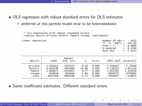
OLS regression with robust standard errors for OLS estimatorI preferred at this permits model error to be heteroskedastic

_cons -.5647368 .2069188 -2.73 0.006 -.9704017 -.159072income .016018 .005606 2.86 0.004 .0050275 .0270085female 1.889675 .2154463 8.77 0.000 1.467292 2.312058

chronic 4.826799 .3001866 16.08 0.000 4.238283 5.415316private 1.916263 .2347443 8.16 0.000 1.456047 2.37648

docvis Coef. Std. Err. t P>|t| [95% Conf. Interval]Robust

Root MSE = 7.4233R-squared = 0.1284Prob > F = 0.0000F( 4, 4407) = 107.01

Linear regression Number of obs = 4412

. regress docvis private chronic female income, vce(robust)

. * OLS regression with robust standard errors

Same coe¢ cient estimates. Di¤erent standard errors.


2. Data Example Comparison of default and robust standard errors

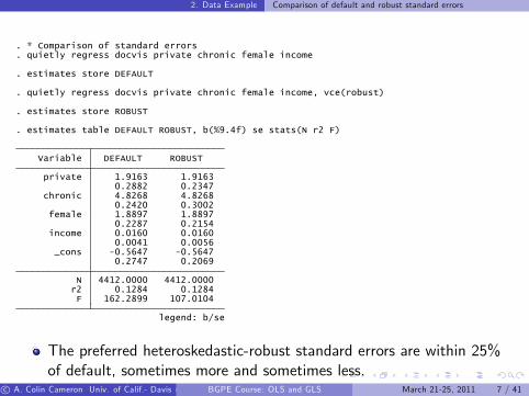
legend: b/se

F 162.2899 107.0104r2 0.1284 0.1284N 4412.0000 4412.0000

0.2747 0.2069_cons -0.5647 -0.5647

0.0041 0.0056income 0.0160 0.0160

0.2287 0.2154female 1.8897 1.8897

0.2420 0.3002chronic 4.8268 4.8268

0.2882 0.2347private 1.9163 1.9163

Variable DEFAULT ROBUST

. estimates table DEFAULT ROBUST, b(%9.4f) se stats(N r2 F)

. estimates store ROBUST

. quietly regress docvis private chronic female income, vce(robust)

. estimates store DEFAULT

. quietly regress docvis private chronic female income

. * Comparison of standard errors

The preferred heteroskedastic-robust standard errors are within 25%of default, sometimes more and sometimes less.


2. Data Example Hypothesis tests

Hypothesis tests can be implemented using Stata command test

H0 : βprivate = 0, βchronic = 0

Ha : at least one of βprivate 6= 0, βchronic 6= 0.

Stata post-estimation command test yields

Prob > F = 0.0000F( 2, 4407) = 165.11

( 2) chronic = 0( 1) private = 0

. test (private = 0) (chronic = 0)

. quietly regress docvis private chronic female income, vce(robust) noheader

. * Wald test of restrictions

Reject H0 at level 0.05 since p < 0.05or 165.11 > F.05(2, 4407) = 3.00 using invFtail(2,4407,.05).


3. Ordinary Least Squares Denition

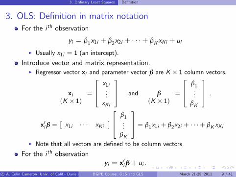
3. OLS: Denition in matrix notationFor the i th observation

yi = β1x1i + β2x2i + + βK xKi + ui

I Usually x1i = 1 (an intercept).

Introduce vector and matrix representation.I Regressor vector xi and parameter vector β are K 1 column vectors.

xi(K 1)

=

264 x1i...xKi

375 and β(K 1)

=

264 β1...

βK

375 .

x0i β =x1i xKi

264 β1...

βK

375 = β1x1i + β2x2i + + βK xKi

I Note that all vectors are dened to be column vectors

For the i th observationyi = x0iβ+ ui .


3. Ordinary Least Squares Denition

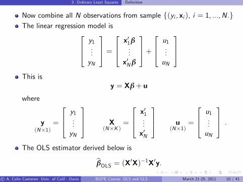
Now combine all N observations from sample f(yi , xi ), i = 1, ...,N.gThe linear regression model is264 y1

...yN

375 =264 x01β

...x0Nβ

375+264 u1

...uN

375This is

y = Xβ+ u

where

y(N1)

=

264 y1...yN

375 X(NK )

=

264 x01...x0N

375 u(N1)

=

264 u1...uN

375 .

The OLS estimator derived below isbβOLS = (X0X)1X0y.c A. Colin Cameron Univ. of Calif.- Davis (Frontiers in Econometrics Bavarian Graduate Program in Economics . Based on A. Colin Cameron and Pravin K. Trivedi (2009,2010), Microeconometrics using Stata (MUS), Stata Press. and A. Colin Cameron and Pravin K. Trivedi (2005), Microeconometrics: Methods and Applications (MMA), C.U.P. )BGPE Course: OLS and GLS March 21-25, 2011 10 / 41

3. Ordinary Least Squares Example

OLS: matrix notation example

Example: N = 4 with (x , y) equal to (1, 1), (2, 3), (2, 4), and (3, 4).

Then y is 4 1 and X is 4 2 with

y =

2664y1y2y3y4

3775 =26641344

3775 ; X =

2664x01x02x03x04

3775 =2664x11 x21x12 x22x13 x23x14 x24

3775 =26641 11 21 21 3

3775 .So (see appendix for detailed computation)

bβOLS = (X0X)1X0y = 4 88 18

1 1227

=

0

1.5

Intercept bβ1 = 0 and slope coe¢ cient bβ2 = 1.5.


3. Ordinary Least Squares Derivation of Formula

Derivation of formula for OLS estimator

The OLS estimator minimizes the sum of squared errors

Q(β) = ∑Ni=1 u

2i = ∑N

i=1(yi x0iβ)

2.

The rst-order conditions (f.o.c.) are

∂Q(β)∂β

= 2∑Ni=1 xi (yi x

0iβ) = 2X0(yXβ) = 0.

Then

X0(yXβ) = 0 from f.o.c.) X0y = X0Xβ K linear equations in K unknowns β) β = (X0X)1X0y if the inverse exists (i.e. rank[X ] = K )

So bβOLS = (X0X)1X0y = ∑Ni=1 xix

0i

1∑Ni=1 xiyi .


4. OLS Properties Summary

4. OLS Properties: Summary

bβOLS is always estimable, provided rank[X ] = K .But properties of bβOLS depend on the true model

I called the data generating process (d.g.p.)

Essential result:I If the d.g.p. is correctly specied andthe error ui is uncorrelated with regressors xi

I Then(1) bβ is consistent for β

(2) bβ is normally distributed in large samples (asymptotically)(3) Variance of bβ varies with assumptions on error ui

F default: ui are independent (0, σ2)F heteroskedastic: ui are independent (0, σ2i )F clustered: ui are correlated within cluster, uncorrelated across clusterF HAC: ui are serially correlated (ui are correlated with ui1)


4. OLS Properties Summary

OLS Properties

If the d.g.p. is y = Xβ+ u then

bβOLS = (X0X)1X0y= (X0X)1X0(Xβ+ u)= (X0X)1X0Xβ+ (X0X)1X0u= β+ (X0X)1X0u= β+ (∑i xix0i )

1 ∑i xiui

So assumptions on xi and ui are crucial.


4. OLS Properties Finite Sample Properties

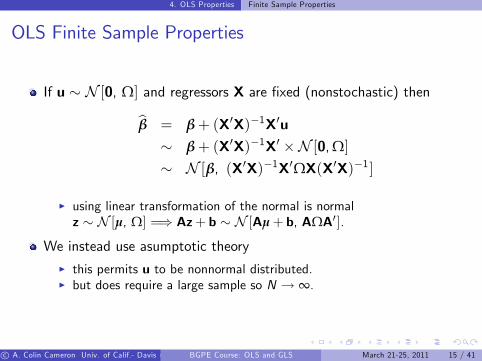
OLS Finite Sample Properties

If u N [0, Ω] and regressors X are xed (nonstochastic) then

bβ = β+ (X0X)1X0u β+ (X0X)1X0 N [0,Ω] N [β, (X0X)1X0ΩX(X0X)1]

I using linear transformation of the normal is normalz N [µ, Ω] =) Az+ b N [Aµ+ b, AΩA0].

We instead use asumptotic theoryI this permits u to be nonnormal distributed.I but does require a large sample so N ! ∞.


4. OLS Properties Consistency

OLS ConsistencyConsistency

I Means that the probability limit (plim) of bβ equals βI That is: lim

N!∞Pr[j bβ βj < ε] = 1 for any ε > 0.

We have (using results below)

plim bβ = plimfβ+ (X0X)1X0ug= plim β+ plim

n(∑i xix0i )

1 ∑i xiuio

= plim β+ plim 1N ∑i xix0i

1 plim 1N ∑i xiui

= β+plim 1

N ∑i xix0i1 0

= β

I plimfAN bN g = plimAN plimbN if the plim0s are constantsI The plims exist using laws of large numbers (as averages)I For plim 1

N ∑i xiui = 0 the key assumption is E[ui jxi ] = 0.


4. OLS Properties Limit Distribution

OLS Limit Distribution

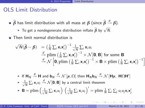
bβ has limit distribution with all mass at β (since bβ p! β).

I To get a nondegenerate distribution inate bβ by pN.Then limit normal distribution ispN(bβ β) =

1N ∑i xix0i

1 1pN

∑i xiuid! plim

1N ∑i xix0i

1 N [0,B] for some Bd! N

h0,plim

1N ∑i xix0i

1 B plim 1N ∑i xix0i

1iI If HN

p! H and bNd! N [µ,Ω] then HNbN

p! N [Hµ, HΩH0]I 1p

N∑i xiui

d! N [0,B] by a central limit theorem

I B = plim1pN

∑i xiui

1pN

∑i xiui0= plim 1

N ∑i ∑j uiujxix0j


4. OLS Properties Asymptotic Distribution

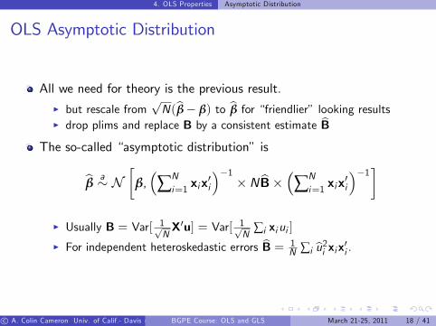
OLS Asymptotic Distribution

All we need for theory is the previous result.I but rescale from

pN(bβ β) to bβ for friendlier looking results

I drop plims and replace B by a consistent estimate bBThe so-called asymptotic distribution is

bβ a N

β,∑Ni=1 xix

0i

1N bB ∑N

i=1 xix0i

1I Usually B = Var[ 1p

NX0u] = Var[ 1p

N∑i xiui ]

I For independent heteroskedastic errors bB = 1N ∑i bu2i xix0i .


4. OLS Properties White Estimate of VCE

White Estimate of VCE

Most often used: requires data to be independent over i .

Then B = plim 1N ∑i ∑j uiujxix0j = plim 1

N ∑i u2i xix

0i .

White (1980) showed that can use bB = 1N ∑i bu2i xix0i .

Yields the heteroskedastic-consistent estimate of thevariance-covariance matrix of the OLS estimator (VCE)

bVrobust[bβ] = ∑Ni=1 xix

0i

1∑Ni=1 bu2i xix0i ∑N

i=1 xix0i

1I bui = yi x0i bβI Leads to heteroskedastic robustor robust standard errors.I In Stata this is option vce(robust) for cross-section commands


4. OLS Properties Other Estimates of VCE

Other Estimates of VCEDefault: Independent homoskedastic errors: V[ui jxi ] = σ2

bV[bβ] = s2 ∑Ni=1 xix

0i

1; s2 =

1N K ∑i bu2i

I Simplication as then B = plim 1N ∑i u2i xix

0i = σ2 plim ∑i xix0i

Cluster robust: Errors correlated within cluster but independentacross cluster.

bV[bβ] = ∑Gg=1 XgXg

01

∑Gg=1 Xgbugbug 0Xg ∑G

g=1 XgXg01

.

I Here observations are stacked in cluster g as yg = Xg β+ ug .I In Stata this is option vce(cluster id) for cross-section commandsI and is option vce(robust) for most xt panel commands.

Heteroskedasticity and autocorrelation (HAC) robust: time seriesI Not covered here but extends White to an MA(q) error.


5. Generalized least squares Overview

5. Generalized least squares (GLS) Overview

OLS is e¢ cient (best linear unbiased estimator) if errors are i.i.d. sothat V[ujX] = σ2I.

I In practice errors are rarely i.i.d.

So we usually do OLS and obtain robust VCE that permitsV[ujX] 6= σ2I

I could be heteroskedastic robust, cluster-robust, HAC, ....

More e¢ cient feasible GLS (FGLS) assumes a model for V[ujX]I yields more precise estimates (smaller standard errors and biggert-statistics)

I but then obtain robust VCE that allows for misspecied model forV[ujX].

I called weighted LS or working matrix LS.


5. Generalized least squares Feasible GLS

Generalized least squares (GLS)Suppose V[ujX] = Ω where Ω is known

I and y = Xβ+ u, E[ujX] = 0 as before.The generalized least squares estimator is e¢ cient:bβGLS = (X0Ω1X)1X0Ω1y.

Derivation:I Premultiply y = Xβ+ u by Ω1/2 so

Ω1/2y = Ω1/2Xβ+Ω1/2u.

I This model has i.i.d. errors sinceV[Ω1/2ujX] = E[(Ω1/2u)(Ω1/2u)0jX] = Ω1/2ΩΩ1/2 = IN .

I Then GLS is OLS in this transformed model:bβGLS = [(Ω1/2X)0(Ω1/2X)](Ω1/2X)0(Ω1/2y)

= (X0Ω1X)1X0Ω1y.


5. Generalized least squares FGLS

Feasible generalized least squares (FGLS)

To implement GLS we need a consistent estimate of Ω.Assume a model for Ω = Ω(γ), estimate bγ p! γ,and form bΩ = Ω(bγ) p! Ω.The feasible GLS estimator (FGLS) is

bβGLS = (X0 bΩ1X)1X0 bΩ1y,

and then bβGLS a Nh

β, (X0 bΩ1X)1i.

Examples:I Heteroskedasticity: V[u2i jxi ] = exp(z0iγ)I Seemingly unrelated equations: yig = x0ig βg + uig , g = 1, ...,G .uig independent over i and homoskedastic with Cov[uig , uih ] = σgh .

I Systems of equations: SUR with βg = β.I Panel data: random e¤ects estimator.


5. Generalized least squares Weighted least squares

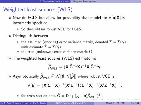
Weighted least squares (WLS)Now do FGLS but allow for possibility that model for V[ujX] isincorrectly specied

I So then obtain robust VCE for FGLS.

Distinguish betweenI the assumed (working) error variance matrix, denoted Σ = Σ(γ)with estimate bΣ = Σ(bγ).

I the true (unknown) error variance matrix Ω

The weighted least squares (WLS) estimator isbβWLS = (X0bΣ1X)1X0bΣ1y.Asymptotically bβWLS a N [β, V[bβ]] where robust VCE is

bV[bβ] = (X0bΣ1X)1(X0bΣ1 bΩbΣ1X)1(X0bΣ1X)1,I for cross-section data bΩ = Diag[(yi x0i bβWLS)2 ].


6. Wald tests and Condence intervals Single restriction

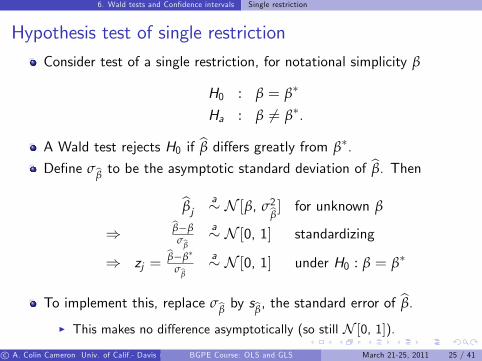
Hypothesis test of single restriction

Consider test of a single restriction, for notational simplicity β

H0 : β = β

Ha : β 6= β.

A Wald test rejects H0 if bβ di¤ers greatly from β.

Dene σbβ to be the asymptotic standard deviation of bβ. Thenbβj a N [β, σ2bβ] for unknown β

) bββσbβ

a N [0, 1] standardizing

) zj =bββ

σbβa N [0, 1] under H0 : β = β

To implement this, replace σbβ by sbβ, the standard error of bβ.I This makes no di¤erence asymptotically (so still N [0, 1]).


6. Wald tests and Condence intervals Single restriction

The Wald z-statistic is

zj =bβ β

sbβa N [0, 1] under H0 : β = β

Implementation by two equivalent methodsI Test using p-values: reject H0 at level 0.05 if

p = Pr[jZ j > jzj j] < 0.05, where Z N [0, 1].

I Test using critical values: reject H0 at level 0.05 if

jzj j > z.025 = 1.96.

Many packages such as Stata use T (N k) rather than N [0, 1]I More conservative (less likely to reject H0)I Exact in unlikely special case that ui N [0, σ2 ].


6. Wald tests and Condence intervals Condence interval

Condence interval

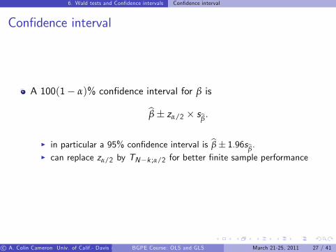
A 100(1 α)% condence interval for β is

bβ zα/2 sbβ.I in particular a 95% condence interval is bβ 1.96sbβ.I can replace zα/2 by TNk ;α/2 for better nite sample performance


6. Wald tests and Condence intervals Multiple linear restrictions

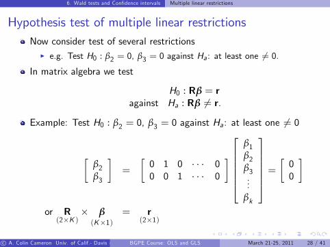
Hypothesis test of multiple linear restrictionsNow consider test of several restrictions

I e.g. Test H0 : β2 = 0, β3 = 0 against Ha: at least one 6= 0.In matrix algebra we test

H0 : Rβ = ragainst Ha : Rβ 6= r.

Example: Test H0 : β2 = 0, β3 = 0 against Ha: at least one 6= 0

β2β3

=

0 1 0 00 0 1 0

2666664

β1β2β3...

βk

3777775 =00

or R(2K )

β(K1)

= r(21)



A Wald test rejects H0 : Rβ = r if Rbβ r di¤ers greatly from 0.

Now Rbβ r is normal as linear combination of normals is normal.bβ a N [β, V[bβ]]

) Rbβ r a N [Rβ r, RV[bβ]R0]) Rbβ r a N [0, RV[bβ]R0] under H0) (Rbβ r)0[RV[bβ]R0]1(Rbβ r) χ2(h) under H0

I The last step converts to chi-square using the result

z N [0,Ω] ) z0Ω1z χ2(dim[Ω]).

To implement this test, replace V[bβ] by bV[bβ].I This makes no di¤erence asymptotically.



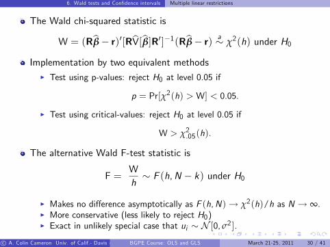
The Wald chi-squared statistic is

W = (Rbβ r)0[RbV[bβ]R0]1(Rbβ r) a χ2(h) under H0

Implementation by two equivalent methodsI Test using p-values: reject H0 at level 0.05 if

p = Pr[χ2(h) > W] < 0.05.

I Test using critical-values: reject H0 at level 0.05 if

W > χ2.05(h).

The alternative Wald F-test statistic is

F =Wh F (h,N k) under H0

I Makes no di¤erence asymptotically as F (h,N)! χ2(h)/h as N ! ∞.I More conservative (less likely to reject H0)I Exact in unlikely special case that ui N [0, σ2 ].



Further test details

Wald test is the commonly-used method to test H0 against Ha.I Estimate β without imposing H0.I Then ask does bβ approximately satisfy H0?

The other two test methods used at times areI Likelihood ratio test: Estimate under both H0 & Ha and compare ln L.I Lagrange multiplier or score test: Estimate under Ha only.I Asymptotically equivalent to Wald under H0 and local alternativesI Choice is mainly one of convenience, though Wald does have theweakness of lack of invariance to reparameterization.

Also as already noted for Wald testI asymptotic theory: use Z and χ2(q)I better nite sample approximation: use T (N k) and F (q,N k)I even better still: bootstrap with asymptotic renement.


7. Simulations OLS consistency and asymptotic normality

7. Simulations: OLS consistency and asymptotic normality

D.g.p.: yi = β1 + β2xi + ui where xi χ2(1) and β1 = 1, β2 = 2.Error: ui χ2(1) 1 is skewed with mean 0 and variance 2.

_cons 1.150439 .6148461 1.87 0.072 -.1090161 2.409894x 2.713073 .5743189 4.72 0.000 1.536634 3.889512

y Coef. Std. Err. t P>|t| [95% Conf. Interval]

. regress y x, noheader

. quietly generate y = 1 + 2*x + rchi2(1)-1 // demeaned chi^2 error

. quietly generate double x = rchi2(1)

. set seed 10101

. quietly set obs 30

. clear all

. * Small sample: parameters differ from dgp values

For N = 30: bβ2 = 2.713 di¤ers appreciably from β2 = 2.000.

I This is due to sampling error as se[bβ2 ] = 0.574.c A. Colin Cameron Univ. of Calif.- Davis (Frontiers in Econometrics Bavarian Graduate Program in Economics . Based on A. Colin Cameron and Pravin K. Trivedi (2009,2010), Microeconometrics using Stata (MUS), Stata Press. and A. Colin Cameron and Pravin K. Trivedi (2005), Microeconometrics: Methods and Applications (MMA), C.U.P. )BGPE Course: OLS and GLS March 21-25, 2011 32 / 41


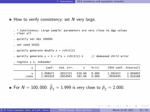
How to verify consistency: set N very large.

_cons 1.005819 .0054945 183.06 0.000 .9950495 1.016588x 1.998675 .0031725 630.00 0.000 1.992457 2.004893

y Coef. Std. Err. t P>|t| [95% Conf. Interval]

. regress y x, noheader

. quietly generate y = 1 + 2*x + rchi2(1)-1 // demeaned chi^2 error

. quietly generate double x = rchi2(1)

. set seed 10101

. quietly set obs 100000

. clear all

. * Consistency: Large sample: parameters are very close to dgp values

For N = 100, 000: bβ2 = 1.999 is very close to β2 = 2.000.



How to check asymptotic results: compute bβ many times.

> reps(1000) saving(chi2datares, replace) nolegend nodots: chi2data. quietly simulate b2f=r(b2) se2f=r(se2) t2f=r(t2) reject2f=r(r2) p2f=r(p2), ///

. set seed 10101

. global numobs 150

. * First define global macro numobs for sample size

. * Results differ from MUS (2008) as MUS did not reset the seed to 10101

. * Run this program 1,000 times to get 1,000 betas etcetera

12. end11. return scalar p2 = 2*ttail($numobs-2,abs(return(t2)))10. return scalar r2 = abs(return(t2))>invttail($numobs-2,.025)9. return scalar t2 = (_b[x]-2)/_se[x]8. return scalar se2 = _se[x]7. return scalar b2 =_b[x]6. regress y x5. generate y = 1 + 2*x + rchi2(1)-1 // demeaned chi^2 error4. generate double x = rchi2(1)3. set obs $numobs2. drop _all1. version 10.1

. program chi2data, rclass

. * Write program to obtain betas for one sample of size numobs (= 150)

. * Central limit theorem

Then look at the distribution of these bβ0s and test statistics.c A. Colin Cameron Univ. of Calif.- Davis (Frontiers in Econometrics Bavarian Graduate Program in Economics . Based on A. Colin Cameron and Pravin K. Trivedi (2009,2010), Microeconometrics using Stata (MUS), Stata Press. and A. Colin Cameron and Pravin K. Trivedi (2005), Microeconometrics: Methods and Applications (MMA), C.U.P. )BGPE Course: OLS and GLS March 21-25, 2011 34 / 41


p2f .5175818 .00914 .499646 .5355177reject2f .046 .0066278 .032994 .059006

t2f .0028714 .0314099 -.0587655 .0645082se2f .0839776 .0005458 .0829066 .0850486b2f 2.000506 .0026649 1.995277 2.005735

Mean Std. Err. [95% Conf. Interval]

Mean estimation Number of obs = 1000

. mean b2f se2f t2 reject2f p2f

p2f 1000 .5175818 .2890325 .0000108 .9997772reject2f 1000 .046 .2095899 0 1

t2f 1000 .0028714 .9932668 -2.824061 4.556576se2f 1000 .0839776 .0172588 .0415919 .145264b2f 1000 2.000506 .08427 1.719513 2.40565

Variable Obs Mean Std. Dev. Min Max

. summarize b2f se2f t2 reject2f p2f

. * Summarize the 1,000 sample means

For S = 1, 000 simulations each with sample size N = 150.

I bβ(1)2 , bβ(2)2 , .... , bβ(1000)2 has distn. with mean 2.001 close to β2 = 2.000I and standard deviation 0.089 close to

p1/150 = 0.082

F using V[bβ2 ] ' (σ2u/V[xi ])/N = (2/2)/150 = 1/150.



Test β2 = 2 using z = (bβ2 β2)/se[bβ2] = (bβ2 2.0)/se[bβ2] to testH0 : β2 = 2.Histogram and kernel density estimate for z1, z2, .... , z1000.

0.1

.2.3

.4.5

Den

sity

-2 0 2 4 6t-statist ic for slope coeff from many samples

Not quite standard normal: N = 150 is still not large enough for CLT.



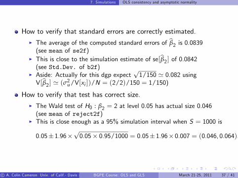
How to verify that standard errors are correctly estimated.I The average of the computed standard errors of bβ2 is 0.0839(see mean of se2f)

I This is close to the simulation estimate of se[bβ2 ] of 0.0842(see Std.Dev. of b2f)

I Aside: Actually for this dgp expectp1/150 ' 0.082 using

V[bβ2 ] ' (σ2u/V[xi ])/N = (2/2)/150 = 1/150)

How to verify that test has correct size.I The Wald test of H0 : β2 = 2 at level 0.05 has actual size 0.046(see mean of reject2f)

I This is close enough as a 95% simulation interval when S = 1000 is

0.05 1.96p0.05 0.95/1000 = 0.05 1.96 0.007 = (0.046, 0.064).


8. Stata commands

8. Stata commands

Command regress does OLSI option vce(robust) for heteroskedastic-robust standard errorsI option vce(cluster clid) for cluster-robust standard errors (withcluster on clid)

For Feasible GLSI command regress [aweight= ] for known or estimatedheteroskedasticity

I command sureg for systems of linear equationsI command nlsur for systems of nonlinear equationsI command xtreg, re for panel random e¤ects.

For hypothesis testsI command test (and nltest for nonlinear hypotheses)


9. Appendix OLS matrix notation example

9. Appendix: OLS matrix notation example

Example: N = 4 with (x , y) equal to (1, 1), (2, 3), (2, 4), and (3, 4).

Vector y and matrix X are

y(41)

=

2664y1y2y3y4

3775 =26641344

3775and

X(42)

=

2664x01x02x03x04

3775 =2664x11 x21x12 x22x13 x23x14 x24

3775 =26641 11 21 21 3

3775 .



Compute bβOLS = (X0X)1X0y :

X0X =1 1 1 11 2 2 3

26641 11 21 21 3

3775 = 4 88 18

.

(X0X)1 =4 88 18

1=

172 64

18 88 4

=

9/4 11 1/2

.

X0y =1 1 1 11 2 2 3

26641344

3775 = 1227.

(X0X)1X0y =9/4 11 1/2

1227

=

108/4 2712+ 54/4

=

0

1.5

.

OLS estimates:I intercept bβ1 = 0 and slope coe¢ cient bβ2 = 1.5.



OLS on intercept and single regressor: yi = β1 + β2xi + ui .

I X0X =1 1x1 xN

264 1 x1...

...1 xN

375 = N ∑i xi∑i xi ∑i x2i

I (X0X)1 = 1N ∑i x 2i (∑i xi )

2

∑i x2i ∑i xi∑i xi N

= 1

∑i x 2i Nx 2

N1 ∑i x2i xx 1

I X0y =1 1x1 xN

264 y1...yN

375 = ∑i yi∑i xi yi

=

Ny

∑i xi yi

I (X0X)1X0y = 1∑i x 2i Nx 2

y ∑i x2i x ∑i xi yixNy +∑i xi yi

= 1

∑i (xix )2

y ∑i x2i x ∑i xi yi∑i (xi x)(yi y)

=

"y bβ2 x

∑i (xix )(yix )∑i (xix )2

#

So bβ1 = y bβ2x and bβ2 = ∑i (xix )(yix )∑i (xix )2

as in introductory course.


day 1a ordinary least squares and gls - a. colin...

Documents