dbTRACEA Scalable Platform for Tracking Information

Filipe Miguel Guerreiro

Thesis to obtain the Master of Science Degree in

Information Systems and Computer Engineering

Supervisor(s): Prof. Paulo Jorge Pires FerreiraProf. Luís Manuel Antunes Veiga

Examination Committee

Chairperson: Prof. Paolo RomanoSupervisor: Prof. Paulo Jorge Pires Ferreira

Co-Supervisor: Prof. Luís Manuel Antunes VeigaMember of the Committee: Prof. Helena Isabel de Jesus Galhardas

October 2016

Acknowledgments

This document was the product of an exhausting year of work as a researcher. It was a journey made

possible thanks to the presence of many people in my life.

I would like to thank in particular Professor Paulo Ferreira. The door to his office was always open.

He consistently allowed this document to be my own work, but steered me in the right the direction

whenever I needed it.

I am grateful to Prof. Luıs Veiga for his insight and valuable comments provided when reviewing this

dissertation.

My sincere thanks to the rest of the team involved in the TRACE project at INESC-ID, namely, Prof.

Joao Barreto, Miguel Costa and Rodrigo Lourenco for valuable technical, infrastructural support, as well

as stimulating discussions and providing important feedback on my work.

I am also thankful to Prof. Helena Galhardas for generously offering her time, good will and valuable

feedback during her role as committee member.

I was fortunate to be conceded a scholarship to support my work, by funds provided to TRACE by the

European Union’s Horizon 2020 research and innovation program under grant agreement No. 635266.

Last but not the least, I would like to thank my mother for supporting and encouraging me throughout

writing this dissertation and over the years.

ii

Resumo

A falta de actividade fısica tem vindo a tornar-se um problema importante na saude publica. Ha um

interesse crescente em influenciar melhores comportamentos de atividade fısica. Benefıcios incluem,

menos trafego, menos poluicao e melhorias na qualidade de vida. Os avancos da tecnologia de sen-

sores tornaram possıvel as iniciativas de rastreamento de grande escala. A iniciativa TRACE e um

projecto Europeu gerido pelo INESC-ID, com o objetivo de incentivar mais pessoas a andar a pe e de

bicicleta. Os participantes sao incentivados atraves do uso de recompensas, tais como descontos e

ofertas.

Este projecto introduz o dbTRACE, uma plataforma geoespacial concebida para armazenar, gerir

e analisar a informacao de localizacao gerada pelos utilizadores. O dbTRACE usa a base de dados

TitanDB para fornecer um modelo de dados e API em grafo. O TitanDB combina o Apache Cassandra,

uma base de dados nao-relacional para o armazenamento distribuıdo dos dados, e o ElasticSearch,

um motor de busca distribuıdo que fornece um ındice para procura geoespacial em todo o cluster. Tra-

jectorias de utilizador sao processadas usando o Barefoot, um servidor de Map-matching que pode ser

distribuido usando a Spark framework. Este processo permite que a informacao seja mais rapidamente

obtida para efeitos de analise estatıstica e validacao de recompensas.

As nossas principais observacoes mostram que o TitanDB e capaz de processar multiplas queries

transacionais, pequenas a medida que o numero de maquinas no cluster aumenta. No entanto, isto nao

e verdade para queries analıticas intensivas. A paralelizacao da carga da query pelas maquinas demon-

stra retornos decrescentes, com uma melhoria de tempo de resposta de 26% de 1 para 2 maquinas,

e apenas de 10% de 4 para 5. Medimos tambem o algoritmo de Map-matching com o nosso data-

set pedestre e bicicleta, obtendo uma precisao media de 90%. Correndo o algoritmo num ambiente

distribuıdo obteve melhorias de 48% com 4 maquinas.

Palavras-chave: Base de dados em grafo, Trajectoria, Distribuicao, Map-matching

iii

Abstract

Physical inactivity has become an important public health issue. There is a growing interest in influenc-

ing better physical activity behaviors. This leads to less traffic, less pollution and quality of life improve-

ments. Advancements in sensor technology have made large-scale tracking initiatives more feasible.

The TRACE initiative is an European project being managed by INESC-ID with the goal of getting more

people walking and cycling. Participants are incentivized by the use of rewards, such as prizes and

discounts.

This dissertation introduces dbTRACE, a geospatial platform designed to store, manage and query

the tracked information generated by the TRACE users. dbTRACE uses TitanDB to provide a graph

API and data model to query data. TitanDB combines Apache Cassandra, a non-relational database for

the distributed storage of data, and ElasticSearch, a distributed search engine that provides an index

for geospatial search over the cluster. Tracked user data is processed using Barefoot, a Map-matching

server that can be distributed using the Spark framework. This process allows information to be quickly

traversed and queried for statistical analysis and reward validation.

Our main findings show that TitanDB does a good job at processing multiple small, transactional

queries as the number of nodes in the system increase. However, this does not hold true to intensive,

analysis queries. Parallelizing the workload of the query explicitly at the client level sees gains with

diminishing returns, with 26% improvement in response time when going from 1 to 2 nodes, but only 10%

when going from 4 to 5. In addition, we measured the Map-matching algorithm against our pedestrian

and biking data-set and obtained an average accuracy of 90%. Running the algorithm in a distributed

environment got gains of almost 48% when using 4 machines.

Keywords: Graph Database, Trajectory, Distributed, Map-matching

iv

Contents

Acknowledgments . . . . . . . . . . . . . . . . . . . . . . . . . . . . . . . . . . . . . . . . . . . ii

Resumo . . . . . . . . . . . . . . . . . . . . . . . . . . . . . . . . . . . . . . . . . . . . . . . . . iii

Abstract . . . . . . . . . . . . . . . . . . . . . . . . . . . . . . . . . . . . . . . . . . . . . . . . . iv

List of Tables . . . . . . . . . . . . . . . . . . . . . . . . . . . . . . . . . . . . . . . . . . . . . . viii

List of Figures . . . . . . . . . . . . . . . . . . . . . . . . . . . . . . . . . . . . . . . . . . . . . ix

1 Introduction 1

1.1 Motivation . . . . . . . . . . . . . . . . . . . . . . . . . . . . . . . . . . . . . . . . . . . . . 1

1.2 Objectives . . . . . . . . . . . . . . . . . . . . . . . . . . . . . . . . . . . . . . . . . . . . . 2

1.3 Challenges . . . . . . . . . . . . . . . . . . . . . . . . . . . . . . . . . . . . . . . . . . . . 3

1.4 Existing solutions . . . . . . . . . . . . . . . . . . . . . . . . . . . . . . . . . . . . . . . . . 4

1.5 Contribution . . . . . . . . . . . . . . . . . . . . . . . . . . . . . . . . . . . . . . . . . . . . 5

1.6 Thesis Outline . . . . . . . . . . . . . . . . . . . . . . . . . . . . . . . . . . . . . . . . . . 5

2 Related Work 6

2.1 Spatial Data . . . . . . . . . . . . . . . . . . . . . . . . . . . . . . . . . . . . . . . . . . . . 6

2.2 Spatial Networks . . . . . . . . . . . . . . . . . . . . . . . . . . . . . . . . . . . . . . . . . 7

2.3 Spatial DBMS . . . . . . . . . . . . . . . . . . . . . . . . . . . . . . . . . . . . . . . . . . . 7

2.4 Spatial Data Mining . . . . . . . . . . . . . . . . . . . . . . . . . . . . . . . . . . . . . . . 8

2.5 Trajectory Pre-processing . . . . . . . . . . . . . . . . . . . . . . . . . . . . . . . . . . . . 9

2.5.1 Noise Filtering . . . . . . . . . . . . . . . . . . . . . . . . . . . . . . . . . . . . . . 9

2.5.2 Stay-Point Detection . . . . . . . . . . . . . . . . . . . . . . . . . . . . . . . . . . . 9

2.5.3 Trajectory Compression . . . . . . . . . . . . . . . . . . . . . . . . . . . . . . . . . 10

2.5.4 Trajectory Segmentation . . . . . . . . . . . . . . . . . . . . . . . . . . . . . . . . . 11

2.5.5 Map Matching . . . . . . . . . . . . . . . . . . . . . . . . . . . . . . . . . . . . . . 11

2.6 Information Security . . . . . . . . . . . . . . . . . . . . . . . . . . . . . . . . . . . . . . . 12

2.6.1 Security Requirements . . . . . . . . . . . . . . . . . . . . . . . . . . . . . . . . . 12

2.6.2 Threat Model . . . . . . . . . . . . . . . . . . . . . . . . . . . . . . . . . . . . . . . 12

2.7 User Privacy . . . . . . . . . . . . . . . . . . . . . . . . . . . . . . . . . . . . . . . . . . . 13

2.8 Trajectory publication . . . . . . . . . . . . . . . . . . . . . . . . . . . . . . . . . . . . . . . 14

2.9 Fraud . . . . . . . . . . . . . . . . . . . . . . . . . . . . . . . . . . . . . . . . . . . . . . . 15

v

2.10 Relational Database Systems . . . . . . . . . . . . . . . . . . . . . . . . . . . . . . . . . . 15

2.11 Non-relational Databases . . . . . . . . . . . . . . . . . . . . . . . . . . . . . . . . . . . . 17

2.11.1 Key-value . . . . . . . . . . . . . . . . . . . . . . . . . . . . . . . . . . . . . . . . . 17

2.11.2 Wide-Column store . . . . . . . . . . . . . . . . . . . . . . . . . . . . . . . . . . . . 18

2.11.3 Document . . . . . . . . . . . . . . . . . . . . . . . . . . . . . . . . . . . . . . . . . 19

2.11.4 Graph . . . . . . . . . . . . . . . . . . . . . . . . . . . . . . . . . . . . . . . . . . . 20

2.12 Database Comparison . . . . . . . . . . . . . . . . . . . . . . . . . . . . . . . . . . . . . . 22

3 Solution 23

3.1 dbTRACE . . . . . . . . . . . . . . . . . . . . . . . . . . . . . . . . . . . . . . . . . . . . . 23

3.1.1 Domain Data . . . . . . . . . . . . . . . . . . . . . . . . . . . . . . . . . . . . . . . 25

3.1.2 Map Data . . . . . . . . . . . . . . . . . . . . . . . . . . . . . . . . . . . . . . . . . 26

3.1.3 dbTRACE API . . . . . . . . . . . . . . . . . . . . . . . . . . . . . . . . . . . . . . 27

3.2 Trajectory Data Pre-processing . . . . . . . . . . . . . . . . . . . . . . . . . . . . . . . . . 29

3.2.1 Stay-Point Detection . . . . . . . . . . . . . . . . . . . . . . . . . . . . . . . . . . . 29

3.2.2 Map-matching . . . . . . . . . . . . . . . . . . . . . . . . . . . . . . . . . . . . . . 29

3.3 Security . . . . . . . . . . . . . . . . . . . . . . . . . . . . . . . . . . . . . . . . . . . . . . 31

3.4 Fraud Countermeasures . . . . . . . . . . . . . . . . . . . . . . . . . . . . . . . . . . . . . 33

3.5 Summary . . . . . . . . . . . . . . . . . . . . . . . . . . . . . . . . . . . . . . . . . . . . . 33

4 Implementation 35

4.1 dbTRACE System . . . . . . . . . . . . . . . . . . . . . . . . . . . . . . . . . . . . . . . . 35

4.2 Web Server . . . . . . . . . . . . . . . . . . . . . . . . . . . . . . . . . . . . . . . . . . . . 36

4.2.1 Handling a Client Request . . . . . . . . . . . . . . . . . . . . . . . . . . . . . . . . 37

4.2.2 Communicating with the Database . . . . . . . . . . . . . . . . . . . . . . . . . . . 38

4.3 Database . . . . . . . . . . . . . . . . . . . . . . . . . . . . . . . . . . . . . . . . . . . . . 39

4.3.1 Schema . . . . . . . . . . . . . . . . . . . . . . . . . . . . . . . . . . . . . . . . . . 39

4.3.2 Indexing Data . . . . . . . . . . . . . . . . . . . . . . . . . . . . . . . . . . . . . . . 40

4.3.3 Distributing TitanDB . . . . . . . . . . . . . . . . . . . . . . . . . . . . . . . . . . . 41

4.4 Database Queries . . . . . . . . . . . . . . . . . . . . . . . . . . . . . . . . . . . . . . . . 44

4.4.1 Reward queries . . . . . . . . . . . . . . . . . . . . . . . . . . . . . . . . . . . . . . 44

4.4.2 Analysis queries . . . . . . . . . . . . . . . . . . . . . . . . . . . . . . . . . . . . . 47

4.5 Trajectory Pre-processing . . . . . . . . . . . . . . . . . . . . . . . . . . . . . . . . . . . . 49

4.5.1 Pre-processing Workflow . . . . . . . . . . . . . . . . . . . . . . . . . . . . . . . . 49

4.5.2 Stay-Point Detection . . . . . . . . . . . . . . . . . . . . . . . . . . . . . . . . . . . 49

4.5.3 Map Matching . . . . . . . . . . . . . . . . . . . . . . . . . . . . . . . . . . . . . . 50

4.6 Security . . . . . . . . . . . . . . . . . . . . . . . . . . . . . . . . . . . . . . . . . . . . . . 52

4.6.1 Web Server . . . . . . . . . . . . . . . . . . . . . . . . . . . . . . . . . . . . . . . . 53

4.6.2 Graph Database . . . . . . . . . . . . . . . . . . . . . . . . . . . . . . . . . . . . . 55

4.6.3 HDFS Cluster . . . . . . . . . . . . . . . . . . . . . . . . . . . . . . . . . . . . . . . 56

vi

4.7 Visualization Application . . . . . . . . . . . . . . . . . . . . . . . . . . . . . . . . . . . . . 60

4.8 Importing OSM Maps . . . . . . . . . . . . . . . . . . . . . . . . . . . . . . . . . . . . . . 61

4.9 Summary . . . . . . . . . . . . . . . . . . . . . . . . . . . . . . . . . . . . . . . . . . . . . 62

5 Results 64

5.1 Index Performance . . . . . . . . . . . . . . . . . . . . . . . . . . . . . . . . . . . . . . . . 64

5.1.1 Graph index . . . . . . . . . . . . . . . . . . . . . . . . . . . . . . . . . . . . . . . . 65

5.1.2 Vertex-centric index . . . . . . . . . . . . . . . . . . . . . . . . . . . . . . . . . . . 65

5.2 Distributed Performance . . . . . . . . . . . . . . . . . . . . . . . . . . . . . . . . . . . . . 66

5.2.1 Response Time . . . . . . . . . . . . . . . . . . . . . . . . . . . . . . . . . . . . . . 67

5.2.2 Consistency Level . . . . . . . . . . . . . . . . . . . . . . . . . . . . . . . . . . . . 68

5.2.3 Replication Factor . . . . . . . . . . . . . . . . . . . . . . . . . . . . . . . . . . . . 69

5.3 Database Query Analysis . . . . . . . . . . . . . . . . . . . . . . . . . . . . . . . . . . . . 70

5.4 Map matching . . . . . . . . . . . . . . . . . . . . . . . . . . . . . . . . . . . . . . . . . . . 71

5.4.1 Accuracy . . . . . . . . . . . . . . . . . . . . . . . . . . . . . . . . . . . . . . . . . 72

5.4.2 Running Time . . . . . . . . . . . . . . . . . . . . . . . . . . . . . . . . . . . . . . . 74

5.4.3 Distributed Performance . . . . . . . . . . . . . . . . . . . . . . . . . . . . . . . . . 75

5.4.4 Space savings . . . . . . . . . . . . . . . . . . . . . . . . . . . . . . . . . . . . . . 76

5.5 Importing Map Data . . . . . . . . . . . . . . . . . . . . . . . . . . . . . . . . . . . . . . . 77

5.6 Summary . . . . . . . . . . . . . . . . . . . . . . . . . . . . . . . . . . . . . . . . . . . . . 77

6 Conclusion 79

Bibliography 81

Appendices 86

A The NoSQL Family . . . . . . . . . . . . . . . . . . . . . . . . . . . . . . . . . . . . . . . . 86

B Urban planner indicators . . . . . . . . . . . . . . . . . . . . . . . . . . . . . . . . . . . . . 87

C Grizzly NIO Handler Implementation . . . . . . . . . . . . . . . . . . . . . . . . . . . . . . 88

D LCS Implementation . . . . . . . . . . . . . . . . . . . . . . . . . . . . . . . . . . . . . . . 89

E Stay-point Detection . . . . . . . . . . . . . . . . . . . . . . . . . . . . . . . . . . . . . . . 90

F Grizzly Access Control . . . . . . . . . . . . . . . . . . . . . . . . . . . . . . . . . . . . . . 91

G Kerberized HDFS Client . . . . . . . . . . . . . . . . . . . . . . . . . . . . . . . . . . . . . 92

H Leaflet code . . . . . . . . . . . . . . . . . . . . . . . . . . . . . . . . . . . . . . . . . . . . 93

I Web Server Authentication using Argon2i . . . . . . . . . . . . . . . . . . . . . . . . . . . 94

J SSL Keystore and Truststore Configuration . . . . . . . . . . . . . . . . . . . . . . . . . . 95

K Parallel Average Trip Distance Query . . . . . . . . . . . . . . . . . . . . . . . . . . . . . . 96

L Map-matching Pedestrian Trips . . . . . . . . . . . . . . . . . . . . . . . . . . . . . . . . . 97

M Spark Execution DAG . . . . . . . . . . . . . . . . . . . . . . . . . . . . . . . . . . . . . . 98

vii

List of Tables

2.1 STRIDE and Security Requirements . . . . . . . . . . . . . . . . . . . . . . . . . . . . . . 14

2.2 A comparison between PostgreSQL, Redis and HBase. . . . . . . . . . . . . . . . . . . . 21

2.3 A comparison between TitanDB and CouchDB. . . . . . . . . . . . . . . . . . . . . . . . . 21

3.1 Checkpoint API . . . . . . . . . . . . . . . . . . . . . . . . . . . . . . . . . . . . . . . . . . 27

3.2 User API . . . . . . . . . . . . . . . . . . . . . . . . . . . . . . . . . . . . . . . . . . . . . 28

3.3 Analyst API . . . . . . . . . . . . . . . . . . . . . . . . . . . . . . . . . . . . . . . . . . . . 28

3.4 Network STRIDE threats . . . . . . . . . . . . . . . . . . . . . . . . . . . . . . . . . . . . . 32

3.5 API Web Server STRIDE threats . . . . . . . . . . . . . . . . . . . . . . . . . . . . . . . . 32

3.6 Storage + Pre-processing cluster STRIDE threats . . . . . . . . . . . . . . . . . . . . . . . 32

5.1 Vertex-centric index performance impact. . . . . . . . . . . . . . . . . . . . . . . . . . . . 66

5.2 Map-matching accuracy. . . . . . . . . . . . . . . . . . . . . . . . . . . . . . . . . . . . . . 74

5.3 Map-matching space savings. . . . . . . . . . . . . . . . . . . . . . . . . . . . . . . . . . . 76

viii

List of Figures

1.1 TRACE model . . . . . . . . . . . . . . . . . . . . . . . . . . . . . . . . . . . . . . . . . . 2

2.1 Spatial Network example . . . . . . . . . . . . . . . . . . . . . . . . . . . . . . . . . . . . 7

3.1 dbTRACE . . . . . . . . . . . . . . . . . . . . . . . . . . . . . . . . . . . . . . . . . . . . . 23

3.2 Logical Domain Data Model . . . . . . . . . . . . . . . . . . . . . . . . . . . . . . . . . . . 25

3.3 Map Data Model . . . . . . . . . . . . . . . . . . . . . . . . . . . . . . . . . . . . . . . . . 26

3.4 Stay-point detection . . . . . . . . . . . . . . . . . . . . . . . . . . . . . . . . . . . . . . . 29

3.5 Map-matching algorithm . . . . . . . . . . . . . . . . . . . . . . . . . . . . . . . . . . . . . 30

3.6 STRIDE Threats in dbTRACE . . . . . . . . . . . . . . . . . . . . . . . . . . . . . . . . . . 31

4.1 dbTRACE Components. . . . . . . . . . . . . . . . . . . . . . . . . . . . . . . . . . . . . . 35

4.2 Grizzly UML Sequence. . . . . . . . . . . . . . . . . . . . . . . . . . . . . . . . . . . . . . 36

4.3 Titan-Cassandra-ES architecture. . . . . . . . . . . . . . . . . . . . . . . . . . . . . . . . . 41

4.4 Trajectory insertion work-flow. . . . . . . . . . . . . . . . . . . . . . . . . . . . . . . . . . . 49

4.5 Application Security Diagram. . . . . . . . . . . . . . . . . . . . . . . . . . . . . . . . . . . 53

4.6 Leaflet Visualization Application . . . . . . . . . . . . . . . . . . . . . . . . . . . . . . . . . 61

4.7 Import OSM Map Workflow. . . . . . . . . . . . . . . . . . . . . . . . . . . . . . . . . . . . 62

5.1 TitanDB indexing options . . . . . . . . . . . . . . . . . . . . . . . . . . . . . . . . . . . . 65

5.2 Response time vs. Number of nodes . . . . . . . . . . . . . . . . . . . . . . . . . . . . . . 67

5.3 Concurrent requests vs. Number of nodes . . . . . . . . . . . . . . . . . . . . . . . . . . . 68

5.4 Response time vs. Consistency level . . . . . . . . . . . . . . . . . . . . . . . . . . . . . . 69

5.5 Response time vs. Replication factor . . . . . . . . . . . . . . . . . . . . . . . . . . . . . . 70

5.6 Urban Planner queries performance . . . . . . . . . . . . . . . . . . . . . . . . . . . . . . 71

5.7 Map matching Sintra bicycle route. . . . . . . . . . . . . . . . . . . . . . . . . . . . . . . . 72

5.8 Map matching snapping effect. . . . . . . . . . . . . . . . . . . . . . . . . . . . . . . . . . 73

5.9 Map matching break. . . . . . . . . . . . . . . . . . . . . . . . . . . . . . . . . . . . . . . . 73

5.10 Map-matching shortcut effect. . . . . . . . . . . . . . . . . . . . . . . . . . . . . . . . . . . 74

5.11 Map matching performance. . . . . . . . . . . . . . . . . . . . . . . . . . . . . . . . . . . . 75

5.12 Distributed Map matching performance. . . . . . . . . . . . . . . . . . . . . . . . . . . . . 76

5.13 OSM Map Import Run-time. . . . . . . . . . . . . . . . . . . . . . . . . . . . . . . . . . . . 77

ix

Chapter 1

Introduction

1.1 Motivation

Populated, urban areas often reach unhealthy levels of pollution. A combination of stationary sources

(e.g. industrial facilities) and mobile sources (e.g. cars and trucks) of pollution can cause respiratory

disease, childhood asthma, cancer, and other health problems [1]. Sedentarism is another risk factor in

urban areas. The World Health Organization (WHO) recommends that every adult aged between 18-64

should do at least 20 minutes of moderate-intensity physical activity each day of the week [2].

Advancements in sensor technology have steadily introduced increases in resolution, while at the

same time, decreasing in cost and size. This in turn has lead to the increasing ubiquity of these devices,

generating a corresponding amount of data, growing at a rate exceeding Moore’s law [3]. In other words,

hardware alone cannot keep up with this trend, requiring the use of software that scales to huge volumes

of data.

This new reality has made large-scale tracking initiatives more interesting. Physical inactivity has

become an important public health issue. There is a growing interest in influencing better physical activity

behaviors. This leads to less pollution, less traffic, better environment and quality of life improvements.

One of the initiatives that has originated from these goals is called TRACE.

The TRACE project,1 led by INESC-ID and partnered with other European organizations (such as

TIS, POLIS, Mobiel 21 and SRM Bologna, among others), aims to improve quality of life in cities by

promoting cycling and walking through the use of reward-based behavior changing tools based on Pos-

itive Drive2, Traffic Snake3 and Cycle-to-Shop.4 In addition, it also aims to use the collected knowledge

to improve urban mobility planning and policy making. Figure 1.1 shows an example of the Cycle-to-

Shop application. The user starts her tracking device to record her trajectory over the city. When the

user finishes her run, she sends her trajectory to a storage back-end, which analyses the information

1http://h2020-trace.eu/2Positive Drive is a game in which users earn points and rewards by using a bike or driving responsibly.3Traffic Snake is a game where school children collectively try to fill a snake board with stickers that they win by traveling to

and from school with eco-friendly transportation.4Cycle-to-Shop is an initiative that encourages participants to ride their bikes near shops, collecting points and earning re-

wards.

1

and informs the user of rewards she may have earned. These rewards, such as gifts or discounts, can

then be redeemed next to stores and shops participating in TRACE. These participants are also called

checkpoints.

Figure 1.1: An example showing the different participants in the TRACE initiative.

This project considers two approaches to trace users. The first considers that the user does not

carry a smartphone, such as children and people with stricter privacy demands. Instead, they can rely

on a simpler device such as a Near-Field Communication (NFC) tag or Low-Energy Bluetooth (LEBT)

reader, that communicates with a device (a beacon)5 installed at each checkpoint, which then can relay

this information back to the storage system.

The second approach considers a user that carries a smartphone device capable of tracking the

user movements over time using a global positioning system. This collected data is called a spatial

trajectory. A spatial trajectory is a set of chronologically ordered points where each point consists

of a geospatial coordinate set and a timestamp. These trajectories offer us information to understand

moving objects and locations. The field that explores and makes sense of trajectory information is called

Trajectory data mining [4].

1.2 Objectives

The goal of this thesis is to design, implement and evaluate a storage system, called dbTRACE, that

handles location information received from TRACE mobile and browser applications. In addition, we

need to support the efficient execution of a variety of analytical queries, such as finding which users meet

the criteria for a reward, as well as statistical queries, such as determining how many users travelled

through a particular route on a given day.

The TRACE initiative is concerned with two types of applications: behavior change and mobility

planning. The former is focused on enhancing certain aspects of cycling and walking promotion cam-

paigns, while the latter is concerned with tracking data analysis for urban mobility planning and policy

making purposes. These applications need to be able to answer queries like the following: origin/desti-

nation, which route, at what time and day, how long, how fast, how often, what are the obstacles,

points of interest or black spots6.

The storage system will need to support the following general properties: scalable - city-level scal-

ability, with potentially millions of users, protect end-user privacy - the system will store and handle5A beacon is a small transmitter which can send and receive information over a local area.6A black-spot is a place where road traffic accidents have historically been concentrated.

2

information on user trajectory data, which is particularly sensitive information, and provide support for

data-mining operations - it must process the received data to remove errors and add semantic value

to increase its usefulness for later data mining analysis.

To implement dbTRACE, there are several geospatial database options available to choose from [5].

NoSQL (No SQL or Not only SQL) database systems have become an increasingly interesting option

for information management, including geospatial data. In order to make a proper selection we provide

an analysis of the different systems available, both relational and noSQL. The main decision factors are:

the maturity of the system, which translates into what type of spatial index is used and what types

of spatial operations are supported, as well as which spatial data types are supported, particularly

points and lines. Furthermore, scalability for both read and write operations and the capability to

store and process large amount of information quickly are essential.

System cost is also a consideration. When considering scalability, there are two main varieties. Ver-

tical scalability and horizontal scalability. Vertical scalability refers to the ability to improve performance

and storage by improving the existing hardware. Horizontal scalability is the ability to distribute both

the data and the computational load over many machines, with no RAM or disk shared among them.

We favor horizontal scalability because it is the most cost-effective measure, even if at the cost of

additional planning and architecture design [6]. In addition, the license used by the technologies is an

important factor, we will favor open-source projects for the ability to modify and adapt the software to fit

our requirements.

1.3 Challenges

Most database systems were not originally designed for geospatial applications. Support has been

growing steadily for the past few years, where some systems have been developing these capabilities

either natively or through extensions. The level of geospatial maturity for each system differs greatly,

however. As such, we must analyze the features each one implements [7]. There has been a great

movement lately by database developers away from relational databases. Developers have found that

the strict transactional properties imposed by these kinds of databases are not a necessity for all appli-

cations, allowing for the implementation of more relaxed systems that are able to scale and work better

on commodity hardware [8]. We must ascertain the viability and advantages of these new solutions.

Scalability is tied to the way the data is stored and how partitionable the system is. As the amount

of information expands it is crucial that data can still be retrieved quickly. Data needs to be managed

in an efficient way. Horizontal scaling capabilities are important for running the system on commodity

hardware and thus, it is more desirable than vertical scaling, where more powerful hardware needs to

be purchased each time the load demands it, leading to higher costs [6].

The interface through which applications and services communicate needs to be simple and well-

known. If the interface is too complicated and/or very unique, developers will need to waste additional

effort to learn it, causing many to avoid our system.

Privacy and security are also critical concerns in location and tracking services. A given trajectory

3

can reveal a great deal of information about a person. Stored data and any communication between the

database and other components must guarantee the user’s identity is not revealed.

In addition, when using spatial trajectory data, we need to deal with a number of issues, such as

noise from the tracking device itself or environmental obstacles such as tall buildings, as well as finding

the most likely sequence of paths and streets the user took, which is useful for further data analysis

and statistics.

1.4 Existing solutions

Complete geospatial systems that aggregate, store, query and display geospatial data are typically

called a Geographical Information System (GIS). The most popular and feature rich GIS systems, such

as ArcGIS (https://www.arcgis.com) and Mapbox (https://www.mapbox.com/) are not open-source.

Open-source solutions such as QGIS (http://www.qgis.org/) and SPRING (http://www.dpi.inpe.br/

spring/english/) use a traditional Relational Database Management System (RDMS), such as Post-

GIS (http://postgis.net/) and SpatiaLite (https://www.gaia-gis.it/fossil/libspatialite/index).

These RDMS have reached their limits in terms of scalability capabilities [9]. They require the acqui-

sition of powerful machines, paying the salaries of the database administrators and invest in caching

technologies such as Memcached (https://memcached.org/). RDMS are too expensive and slow for

the huge data requirements of TRACE.

To serve these emerging scalability requirements, new systems were designed. Systems that scale

to a large number of nodes without degrading the quality of service and at a low cost. These sys-

tems are NoSQL. NoSQL systems have been classified by several different taxonomies. The most

commonly used is by data model, provided by Cattell [9], which divides systems into Key-Value, Wide-

Column, Document and Graph. There are currently hundreds of different solutions, each with different

support of geospatial data. Examples of database systems with geospatial support include CouchDB

(http://couchdb.apache.org/), MongoDB (https://www.mongodb.com/), Neo4j (https://neo4j.com/)

and TitanDB (http://titan.thinkaurelius.com/).

There is also a need to visualize this information in a way that users can find important information

more easily. Commercial solutions can do this easily, such as the ArcGIS Visualization tool, as well

as online APIs such as Google Maps API and Bing Maps API, which have a server-side geocoding,

search and routing integration. With regards to open-source software, the most popular are Leafletjs

(http://leafletjs.com/) and OpenLayers (http://openlayers.org/). These are JavaScript libraries

that can run both on desktop and on mobile devices.

Sensor data received (e.g. GPS points) often contains errors which first needs to be processed

in order for the data to be consistent and useful for further analysis. This project is concerned with

time-based position data, i.e., trajectories. Several techniques exist that try to fix and draw prelim-

inary semantic meaning from trajectory data. By far, the most difficult and important technique in

trajectory preprocessing is Map-matching, which is the process of matching the trajectory points to

the underlying map network (we give a more detailed overview of the different techniques in Chap-

4

ter 2). There already exist software solutions that implement the current state-of-the-art algorithms, ei-

ther as a stand-alone server format, such as OSRM (http://project-osrm.org/) and Barefoot (https:

//github.com/bmwcarit/barefoot), or as an online, commercial API, such as TrackMatching (https:

//mapmatching.3scale.net/) and GraphHopper (https://graphhopper.com/). Out of the open-source

options, Barefoot has the advantage of being scalable through the use of parallel processing frame-

works (such as Hadoop and Spark), while OSRM has the benefit of having several transport modes

(walk, cycle, car) profiles that help in a more accurate map matching procedure.

dbTRACE aggregates different technologies from all these fields in order to offer a solution that fits

the requirements laid out by TRACE.

1.5 Contribution

This work presents the storage module designed to address the prevalent issues of TRACE, called

dbTRACE. dbTRACE is a platform for storing city road map information, user tracking information and

providing tracked data for analysis. We identify the main contributions of this thesis as follows:

• Analysis of the state-of-the art systems and techniques related to the geospatial field;

• An architecture proposal of the system as a response to the identified functional and non-functional

requirements;

• System implementation including a distributed storage component using TitanDB and its relevant

queries, a distributed Map-matching application using Spark and a visualization component using

Leaflet;

• Qualitative assessment of each system component.

1.6 Thesis Outline

This document is structured into 6 major chapters. Chapter 2 (Related Work) introduces the basic con-

cepts in dealing with geospatial information and security and privacy concerns, as well as a thorough

analysis of the state of the art in geospatial database systems. Chapter 3 (Solution) presents the de-

sign of the dbTRACE system. Chapter 4 (Implementation) describes the implementation details of the

proposed system. Chapter 5 (Results) shows the execution results of dbTRACE obtained with an exper-

imental evaluation, assessing the efficiency of the proposed solution on a set of representative set-ups.

Lastly, Chapter 6 (Conclusions) discusses the research performed, summarizing the contributions made

and gives directions for future work based on what was achieved during the project.

5

Chapter 2

Related Work

In this chapter, an overview of the concepts required to understand the rest of this thesis is presented.

Sections 2.1 (Spatial Data), 2.2 (Spatial Networks) and 2.3 (Spatial DBMS) give an introduction

to the core concepts and technologies that give support to the storage and manipulation of geospatial

trajectories. Geospatial trajectories are the main source of data for this project.

Section 2.4 (Spatial Data Mining) provides a look at what techniques exist to analyze and extract

information from trajectory data. This is important for modeling our data and choosing our technologies,

in order to support a range of applications used by analysts and urban planners.

Section 2.5 (Trajectory Pre-processing) analyzes the techniques that handle trajectory data before

it can be used for analysis. These techniques range from error/noise correction, data compression to

semantic information extraction.

Sections 2.6 (Information Security), 2.7 (User Privacy), 2.8 (Trajectory Publication) deal with the

different techniques needed to keep user information secure and private according to Data Protection

legislation (such as the Dutch Data Protection Act and the European General Data Protection Regula-

tion).

Section 2.9 (Fraud) looks at ways to protect the system (which may include monetary or rewarding

incentives) from abuse. In particular, we overview the types of attacks specific to geospatial systems.

We provide a review of the current field in database technologies in Sections 2.10 (Relational

Databases), 2.11 (Non-relational Databases) where we look at some of the best solutions to our

requirements. We finish the chapter with Section 2.12 (Database Systems Comparison), where we

choose the storage technology for dbTRACE and explain the reasoning behind the choice.

2.1 Spatial Data

Spatial data, also known as geospatial data, is information about a physical object that can be rep-

resented by numerical values in a geographic coordinate system. It represents the location, size and

shape of an object on planet Earth such as a building, lake, mountain or town. Spatial data may also

include attributes that provide more information about the entity that is being represented. The Open

6

Geospatial Consortium (OGC) and ISO 19125 have defined a structure for a spatial data type. The

Geometry type is comprised of point, curve, and geometry collection types that can be combined to

represent virtually any spatial object [10, 11].

2.2 Spatial Networks

Transportation and mobility networks, such as roads, aqueducts and railways, are conceptually repre-

sented by spatial networks. Spatial networks are graphs whose nodes and edges are located in a

space equipped with a metric, i.e. distance function, such as the Euclidean distance1 [12].

An urban spatial network can be modeled with the nodes representing intersections and junctions,

while the edges represent segments of roads and streets between these nodes [13].

Figure 2.1: A spatial network example showing a road network (Toulouse OpenData).

2.3 Spatial DBMS

A Spatial Database Management System (SDBMS) is a database optimized to store and query data that

represents objects defined in a geometric space [14]. That is, it is a database system that offers spatial

data types in its data model and query language, as well as providing spatial indexing and efficient

algorithms for spatial operations [10, 11].

A Spatial Data Type, such as points, lines, and polygons, allow the database to provide a funda-

mental abstraction for modeling the structure of geometric entities in space.

The second component of the spatial database is the Spatial Index. Virtually all databases include

indexing schemes to enable quick look-up and retrieval of the data. There are several different indexing

schemes that are well suited for spatial data. Examples of these are B trees, R trees and Z-order curve

function. The primary difference between these indexing schemes is the way that the data is partitioned

[15].

The spatial data type and spatial index enable the storage and accessing of data. To manipulate

and determine the relationship between spatial data, Spatial Operators are needed. There are three

1The Euclidean distance or Euclidean metric is the straight-line distance between two points in space.

7

categories of operators: functions, predicates and measures. Spatial functions allow for geometry ma-

nipulation, such as creating a buffer around an object, or transforming a curve into a line. Spatial pred-

icates, such as lintersectsr or area(r) > 1000, enable for true or false queries to the dataset. Spatial

measurements can compute the area of a polygon or the length of a given line [15].

2.4 Spatial Data Mining

Spatial data mining is the process of discovering patterns and knowledge in large, spatial data sets.

Pattern discovery includes finding and grouping similar sets of objects (called cluster analysis), finding

unusual records (anomaly detection) and finding if/then relationships between data (association rule

learning).

TRACE is concerned with the tracking and storage of users. Tracking devices carried by users

generate the evolution of their position over a period of time. This generated information is called a

trajectory [16, 17]. Trajectory data mining is a branch of the spatial data mining field. Trajectories offer

much information in understanding moving objects and locations, enabling a broad range of applications

in urban planning, intelligent-transportation systems and location-based social networks.

According to Zheng [18], trajectory data mining can be split into four categories: Trajectory uncer-

tainty, Trajectory Pattern Mining, Trajectory Outlier Detection and Trajectory Classification.

• Trajectory Uncertainty: Tracking devices can only update the location of a moving object at

discrete times. The distance between updates can be so big as to leave the route between the two

points uncertain. Techniques to do this involve path inference, which consists of constructing the

most likely routes based on similar routes.

• Trajectory Pattern Mining: This category is concerned with analyzing the mobility patterns of

moving objects. There are 4 categories of pattern mining. Moving-together pattern mining tries

to discover groups of objects moving together for a specified time period. Trajectory clustering

attempts to group similar trajectories, or sub-trajectories (parts of a trajectory) together to find

common trends. Periodic pattern mining tries to find activities that occur periodically, such as

weekend shopping or daily commute. Sequential pattern mining focuses on finding the sequen-

tial pattern from a single trajectories or multiple trajectories, such as finding a group of tourists

traveling through a common sequence of locations in a similar time interval.

• Trajectory Outlier Detection: Outliers, or anomalies, are items (trajectories or segments of tra-

jectories) that are significantly different from other items. In addition, events or observations may

also be discovered from trajectory data, such as traffic congestion or accidents.

• Trajectory Classification: This subset is concerned with adding semantic value to data, classify-

ing trajectories or segments into categories. These categories can be activities (such as dining or

hiking) or different transportation modes, such as walking or driving.

8

2.5 Trajectory Pre-processing

Data received from sensors often has errors that need to be corrected. The size of a trajectory can often

be a problem due to high sampling rate of devices, leading to overuse of storage space and processing

time. A sequence of GPS points may not have enough semantic meaning for applications. Furthermore,

it may be difficult to distinguish which road certain sequences of points belong to, due to overpasses and

crossings. The ability to solve these issues is fundamental for many trajectory mining tasks. Trajectory

Pre-processing encompasses five basic techniques: noise filtering, stay point detection, trajectory

compression, trajectory segmentation and map matching [19].

2.5.1 Noise Filtering

Sensor noise and other factors, such as receiving poor positioning signals in city spaces, can lead to

point errors that deviate several hundred meters away from its true location. These noise points need to

be filtered before beginning a mining task. Current solutions fall into three categories: mean (or median)

filter, Kalman and particle filters, and heuristics-based outlier detection [19].

Mean (or Median) Filters work as follows. We take a measured point z and estimate its value using

the mean (median) of the n − 1 predecessors in time. The median filter is more robust when handling

extreme errors. Both work well until the sampling rate of the trajectory is very low (as in, several hundred

meters of distance between points).

Kalman and Particle Filters improve upon the previous filters by adding estimates of motion. These

are effective even in trajectories with a low-sampling rate. Kalman and Particle filters work in steps.

During the initialization step, P particles are generated from the initial distribution. They start with zero

velocity and are clustered around the initial location with a Normal distribution. In the second step, a

dynamic model simulates how a particle would change in one time-step. The third step calculates the

importance weights of each particle. A more detailed explanation of these methods can be found at Lee

and Krumm (2011) [20].

Heuristics-based Outlier Detection work by removing noise points directly from a trajectory by

using outlier detection algorithms. First, the method calculates the travel speed of each point in the

trajectory based on pairs of points. From this list of segments, speeds larger than a given threshold

are cutoff. The method may go further and remove points that have less neighbors in a distance of d

compared to a p proportion of the points in the entire trajectory. These thresholds values d and p give

the heuristics name to the method.

2.5.2 Stay-Point Detection

Stay points are points that denote locations where the user has stayed for a while, such as shopping

malls and tourist attractions. There are two types of stay points. The first is the single point stay-point,

where the individual remains stationary for over a time threshold. This tends to occur when the individual

enters a building and loses the satellite signal until returning to the outdoors. The second is the most

9

common, where users walk around within a small spatial region for over a time threshold. This tends to

occur when the individual wanders around some places, like a park or a campus [18].

These stay points can turn a trajectory as a series of time-stamped spatial points to a series of

meaningful places. This in turn, is used for a variety of applications such as travel recommendation, taxi

recommendation, destination prediction and method of transport used.

The first stay-point detection algorithm was proposed by Li et al. [21]. Stay-points can be detected by

seeking the spatial region where the user spent a period exceeding a certain threshold. More concretely,

they take a candidate point and see if its successor is within a given distance and time-span threshold

(200m and 30 minutes for instance). They keep checking the following successors in the trajectory until

the one passes the threshold, identifying the stay-point. This algorithm was then improved by Yuan et

al. [22] to identity common points of interest by looking at different trajectories’ stay-points and using a

density based clustering method.

2.5.3 Trajectory Compression

Devices can generate trajectories with time-stamped geographical coordinates every second for a mov-

ing object. This costs a lot of computing and storage in the long run. To address this issue, there have

been two categories of compression strategies proposed to reduce the size of trajectories without com-

promising much the precision of the new representation. The first is offline compression (or batch mode),

which compresses a trajectory after it has been fully generated. The other is online compression, which

compresses the trajectory at run-time as it is generated.

Offline Compression can be accomplished with the Douglas-Peucker algorithm [23]. The idea is to

replace the original trajectory with an approximate line segment. If the distance from the line to any point

is greater than a specified error threshold, the segment is partitioned between the point contributing the

biggest error. This is done recursively until every segment is under the error requirement. The complexity

of this algorithm is O(N2), but can be improved to O(NlogN) using the modified version introduced by

Hershberger and Snoeyink [24].

Online Compression methods are divided into two categories. The first are the window-based

algorithms, such as the Sliding window and the Open window algorithms, while the second are based

on the speed and direction of a moving object. In the Sliding window algorithm, points are inserted into

a growing window with a line segment until the approximation error exceeds some bound. The Open

window algorithm chooses the point with the maximum error in the window using Douglas-Peucker. This

point is then used to approximate its successors. The moving object speed and direction-based methods

such as Potamias et al. [25] work in the following way. They check the angle and distance from one

point to the next based on the speed (taking into account the previous two points) of the object. If the

point is outside of those parameters, it is discarded from the trajectory.

10

2.5.4 Trajectory Segmentation

In many data mining operations, such as trajectory classification and clustering, we need to divide

trajectories into segments for further processing. There are three types of segmentation methods [19].

The first type is based on time intervals. If the time interval between two points is greater than a

given threshold, a trajectory is divided into two parts between them.

The second is based on the shape of the trajectory. It divides the trajectory when the angle of

between the current direction and the next point passes a given threshold, called turning points. We can

use algorithms such as the Douglas-Peucker for instance, to identify these points.

The third category is based on the semantic meaning of points in a trajectory. Zheng et al. [26]

segment trajectories based on the mode of transport used. To do this, they determine the stay-points in

the trajectory to divide it into segments. The intuition is that, to switch between mode of transport, the

user must stop and transition slowly between modes (when getting off and on). They then take each

segment and categorize their points into walk points and non-walk points based on their speed and

acceleration. There may be cases where a car slows down in traffic and is recognized as walk mode

or vice-versa when a walk point exceeds a speed threshold. To avoid this, a segment is merged into

its backward segment if that segment is small in either length or time than a certain threshold. If it is

over that threshold it is deemed a certain segment. Uncertain segments are merged into one non-walk

segment if the number of consecutive uncertain segments exceeds a certain amount (three for instance).

The intuition for this is that users typically do not switch transport modes within short distances. Later,

the exact transport mode is determined from features in each segment.

2.5.5 Map Matching

Map matching is the process of converting a sequence of latitude/longitude points into a sequence of

road segments. Knowledge of the road a user is or was is important for tasks such as navigation and

data mining [27].

Algorithms can be divided into four categories. The first is the geometric group of algorithms.

Matching is done by mapping individual GPS points to the nearest map point or edge. They are the

fastest algorithms, but lead to topological problems since they do not take into account the connectivity

of the road network. The second category is the topological group which fixes this problem. Matching

is done in two steps; the first is the initial matching process, which takes the first point(s) of the trajectory,

and finds candidate starting links with a score based on their distance. In the second stage, they will

continue matching points in the trajectory, and for each candidate path, choose the next link/edge in

the map data that improves the score [28]. The third is the probabilistic group, which considers noisy

and low-sampling sequences by creating error regions around points (calculated from the device) and

chooses the most likely link based on factors such as speed and direction [29]. Finally, there are the

advanced group of algorithms which use combinations of probabilistic and topological approaches.

Newson and Krumm [30] use a Hidden Markov Model (HMM)2 which is robust to noisy and sparse

2A Markov model is a model used to represent randomly changing systems where it is assumed that future states depend only

11

trajectory data. In their model, the states are the road segments and the state measurements are the

location measurements. Pereira et al. [31] focus on a genetic algorithm that adds non-mapped paths

into the database when their algorithm fails to properly match a trajectory.

2.6 Information Security

The security of systems with sensitive information is crucial. Situations where data becomes damaged

or stolen can effectively render the system obsolete, and the company that holds it liable for damages.

2.6.1 Security Requirements

The heart of information security, often called the CIA-triad, involves 3 building blocks [32]: confiden-

tiality, integrity and availability.

• Confidentiality is the process of making sure that data remains private and confidential, and that

it cannot be viewed by unauthorized users or eavesdroppers who monitor the flow of traffic across

a network.

• Integrity is concerned with the prevention of improper (accidental or deliberate) modification of

information during transit or in storage.

• Availability is the focus on making sure the legitimate users of system do not lose access to the

service. This includes the prevention and recovery against Denial of Service (DoS) attacks and

exploits for hardware and software errors.

The CIA taxonomy has been extended by Microsoft to adapt to the Web Service environment, adding

authentication, authorization and non-repudiation.3

• Authentication is the process that proves the identity of the user of the system (also called a

principal).

• Authorization is the process after Authentication. It ensures that a user has sufficient rights

to perform the requested operation and preventing those without sufficient rights from doing the

same.

• Non-repudiation (or Accountability) is the process that establishes responsibility for actions or

events occurred, tracing actions back in time to the users.

2.6.2 Threat Model

Applying the above measures to complex systems requires identifying what threats exist to the system

in question [33].

on the present state and not on the sequence of events that preceded it. They are referred to as hidden since the actual systemstates can only be observed by a sequence of emissions (measurements).

3Web Service Security https://msdn.microsoft.com/en-us/library/ff648318.aspx

12

Enumerating the threats to a system helps to apply realistic security requirements. This technique is

called Threat Modeling. One common model, developed by Microsoft, is called the STRIDE model [34].

STRIDE is an acronym for grouping the different threats into six categories: Spoofing, Tampering,

Repudiation, Information disclosure, Denial of service and Elevation of privilege. Each of these

threats violates one of the Security Requirements as shown in Table 2.1.

Spoofing refers to accessing and using another user’s credentials. In order to protect against these

attacks, we need Authentication measures. These involve the use of of digital signatures4, strong

password policies and multi-factor authentication (the different methods are what you know, what you

have and what you are, e.g., password, token and bio-metrics, respectively).

Tampering relates to unauthorized changes to data. To defend against this, we need to assure the

Integrity of the data. This is accomplished by using hashing techniques and Message Authentication

Codes (MAC) (a hash function that uses a secret key shared between parties to guarantee that the

message was not created by a third-party).

Repudiation means that the user can deny having performed an action if the other party has no way

to prove without question it was done by that user. Non-repudiation is usually assured using logging

trails and auditing, combined with the use of digital signatures.

Information disclosure is the access of information by individuals without proper authorization to do

so. To prevent this, Confidentiality measures need to be implemented. This involves using encryption

schemes for protecting data in transit and in storage.

Denial of service refers to limiting the availability of the system to service users. Availability mech-

anisms involve using off-the-shelf filtering mechanisms such as firewalls (e.g. packet filters) and redun-

dant machines to handle the extra load.

Elevation of privilege is the gain of privileged access, obtaining the ability to compromise or de-

stroy the entire system. To counter this, Authorization mechanisms are needed, such as the use of

permission and access control checks, combined with user input validation.

2.7 User Privacy

A number of ethical requirements apply to research data when that data pertains to human beings. The

right to privacy is protected by Data Protection Acts and Online Privacy Laws that must be upheld.

The ICO (Information Commissioner’s Office) (https://ico.org.uk/), one of the member offices of

the EU responsible for upholding the European Data Protection Directive, identifies the following key

techniques for anonymizing data:5

• Data Masking. This involves stripping out personal identifiers such as names, to create a dataset

in which no personal identifiers are present.

4A digital signature is a technique used to detect forgery or tampering. The sender uses a signing algorithm, given a messageand a private key, to produce a signature. The recipient uses signature verifying algorithm that, given the message, public key andsignature, can verify the message’s authenticity.

5Reference, http://datalib.edina.ac.uk/mantra/protectionrightsandaccess/

13

Table 2.1: STRIDE and Security RequirementsTHREATS VIOLATESSpoofing Authentication

Tampering IntegrityRepudiation Non-repudiation

Information Disclosure ConfidentialityDenial of service Availability

Elevation of privilege Authorization

• Pseudoanoymization. De-identifying data so that a pseudonym reference is attached to a record

without the individual being identified.

• Aggregation. Data is displayed as totals, instead of single records linking specific individuals.

Small amounts of data are often blurred or excluded because they present greater risk of identifi-

cation. Sampling or mixing record data are often used in these cases.

• Derived data items and banding. This technique involves deriving data from the source data by

producing coarser descriptions of values than in the original dataset. For example, replacing dates

of birth by the year or addresses by areas.

Privacy in location-based services is not as simple as hiding the identifiers of the user (e.g. name,

social security number) [35]. Having information on trajectory data together with other sources of infor-

mation can often expose a user’s identity. Next, we take a look at the main methods for anonymizing

trajectory data.

2.8 Trajectory publication

User location trajectories can be very useful for business analysis and city planning. Making this infor-

mation available to third-parties must ensure user anonymity. The article written by Chow [36] discusses

several approaches to anonymize trajectory data. These approaches are based on the notion of k-

anonymity. K-anonymity [37] tries to protect privacy by taking the attributes that can identify a given

user (called a quasi-identifier), and making it indistinguishable from k-1 other users. This means that for

each quasi-identifier, there are k users with the same one, otherwise they become distinguishable.

The Clustering-based approach works by grouping trajectories made within the same time period,

and with a maximum euclidean distance d from each other. These trajectories are then represented by

a single cluster trajectory that takes the average position of each trajectory. A blurring bounding box of

radius d is created around this new trajectory, representing the uncertainty factor.

In the Generalization-based approach, there are two phases. In the first phase, called the Anonymity

phase, the set of trajectories are divided into groups of k-anonymity trajectories. The next phase, called

the Reconstruction phase, takes the trajectories within each group and recombines them. These new

trajectories can then be made public.

14

The Suppression-based approach takes the original trajectories and an adversary which has part

of the trajectories information. The original trajectories are then suppressed, i.e. the points that can be

used to uniquely identify an individual are removed until the trajectories cannot be singled out using the

adversary’s trajectory information.

The Grid-based approach’s basic idea is to construct a grid on the system space, with a resolution

proportional to the privacy degree desired. Each point is then represented as the grid cell it falls in,

blurring the precision of the location.

Most trajectory data mining operations, such as Outlier Detection[38] and Trajectory Pattern Mining[17],

require a street-level granularity to be useful. Since these operations are a requirement to this project,

we cannot use these trajectory anonymization methods. Since the only users with access to this data

are limited to urban planners, pseudoanonymization is a good choice, removing any form of direct iden-

tification, save for cross-reference identification.

2.9 Fraud

Systems are always susceptible to fraudulent activity. Systems which reward users even more so. The

TRACE project, which provides real-world rewards to the user when a user checks in at a certain venue

or location, is susceptible to Location-based fraud attacks.

He et al. [39] calls these kind of attacks ”Location cheating”. To protect against these, the authors

identify three types of attacks. The first is called Frequent check-ins, where a user tries to repeatedly

check-in the same venue multiple times in a short period. The second is the Super human speed,

where a user checks into locations that are very distant from one another. The third is Rapid-fire

check-ins, where a user checks-in at venues which are close to one another in a quick succession.

Foursquare6 (https://www.foursquare.com/) used simple per-user mechanisms such as limiting check-

in frequency, excluding locations that require surreal speeds to be achieved and denying check-ins at

different business within a certain time-distance of each other.

However, these measures are not enough. He et al. successfully evaded the Foursquare system

through the use of an automated attack which spoofed the device’s GPS positioning system and sim-

ulated a user passing different venues with realistic speed and distance constraints. He et al. [39],

Carbunar et al. [40], Saroiu et al. [41] propose different solutions to counteract this type of attack, how-

ever, they rely on the tracking device or on the venu-side network infrastructure, which is outside of the

scope of this thesis.

2.10 Relational Database Systems

The most common and established database storage model for several decades has been the relational

data model. This term was first introduced by Codd [42] in 1969. Software that implements this model

6Foursquare is a local search and discovery service for places of interest.

15

is called a Relational DataBase Management System (RDBMS). A relational database is a set of tables,

each table with one or more attributes per column. Each row with a unique instance of attributes.

Support for geospatial capabilities was added fairly recently. Microsoft SQL Server added a few

features in version 2008 [43], and added significantly again in version 2012 [44]. PostgreSQL also

became spatially enabled with the PostGIS library support starting in 2005.

Because of their rich set of features, query capabilities and transaction management, RDBMSs fit

almost every possible database task. However, their feature richness is also their weakness. Relational

databases do not scale well. When the processing requirements exceed the hardware limits of a single

machine, the data has to be replicated and distributed across a cluster of machines. Guaranteeing

ACID7 properties places a bottleneck on performance. Joining tables across distributed computers is

difficult and time-consuming. Since RDBMS have to guarantee durability, logs are left on the disk for

every operation, which places a severe load on the I/O.

Unstructured data is another problem. Dynamic and ad-hoc data without a predefined model lead to

irregularities and ambiguities which are difficult to store in a relational data model [45].

Out of the open-source database systems, we take a look at the most mature and developed solution

available, based on the cross comparison of Obe [46] and Kushim [47].

PostgreSQL

PostgreSQL is an open-source object-relational8 database. It was written in C and first released nearly

20 years ago.

In terms of scalability, PostgreSQL has a customizable replication model. Starting in version 9.0, a

hot standby architecture was implemented, where a server can send write-ahead logs to other replicas

asynchronously, and those replicas can be read from, increasing read performance. A warm stand-by

architecture is also available, where write-ahead logs are sent to replicas used for fail-over situations.

A multi-master replication is available as well starting with version 9.4, with writes being performed to

individual servers, and then asynchronously merging the changes through conflict rules or user input.

A few more replication strategies are available9, and even more can be added through available open-

source packages, such as Londist, Bucardo and SymmetricDS.

Geospatial capabilities were first added in 2001 with the PostGIS library. PostGIS follows the Simple

Features standard of the OGC. It implements geometries such as Points, LineStrings and Polygons.

Operations such as determining length, area and intersections are available. An R-tree and Generalized

Search Tree (GiST)-tree implementation is also available for inserting, deleting and quickly retrieving

geometries.

PostGIS can also be combined with GeoServer to view and edit the spatial map. It also supports

importing ESRI shapefiles using the shp2pgsql loader.

7ACID stands for Atomicity, Consistency, Isolation, Durability. They are a set of properties that guarantee that databasetransactions (i.e. single logical operations on the data) are processed reliably.

8Similar to relational databases, but offers an object-oriented database model, with objects and inheritance being supportedin the schema and query language.

9Full list of replication strategies for Postgres, http://www.postgresql.org/docs/current/\static/different-replication-solutions.html

16

2.11 Non-relational Databases

Non-relational databases have been around since the late 1960s, including graph, hierarchical and

object-oriented databases [48]. The NoSQL (Not Only SQL) movement started with Google’s BigTable

(2004) and Amazon’s Dynamo (2007) with the intent of offering scalability and availability beyond the

relational model [7].

In this work, interest lies mostly with the spatial capabilities of each system. These capabilities were

chosen based on ISO SQL/MM [49] and the OGC standard [10]:

• Data types: support for the datatypes such as Point, Line, Surface, Curve, Polygon, etc.

• Indexing: indexing techniques are used to speed up certain kinds of queries. Index structures

such as quadtree, R tree, geohashing are more appropriate for spatial indexing.

• Functions: support for the functions listed by the standards, namely: property retrieval (length,

boundary, etc.), comparison (intersects, touches, contains, etc.) and support for spatial analysis

(union, difference, buffer, etc.).

The following sections give a brief overview of the NoSQL world according to a popular taxonomy

given by Sharma [50] and Cattell [9]. An illustration of some of the more relevant technologies according

to this model can be seen in the Appendix A.

This is not a comprehensive listing, there are many more NoSQL system databases, but we focus

on the most popular solutions10 with the most robust geospatial capabilities. Tables 2.2 and 2.3 are

also available for a condensed side-by-side comparison of the different database options. Afterwards,

a representative system will be chosen based on maturity, the criteria mentioned here and whether it is

open-source or not.

2.11.1 Key-value

Key-value databases store items as alpha-numeric identifiers (keys) and associated values in simple,

standalone tables (referred to as hash tables). The values may range from simple text strings to more

complex lists and sets. Data searches can usually only be performed against keys, not values, and are

limited to exact matches. Key-value DBs use the hash function as the index, so they are slower when

searching ranges.

Examples of open-source, Key-value databases are: Memcached (https://memcached.org/), Redis

(http://redis.io/) and Riak (https://github.com/basho/riak). Out of these, the solution with the

most features and maturity is Redis. Memcached does not have spatial support, while Riak is less

performant than Redis and its masterless replication method uses a commercial license [51].

10Based on http://db-engines.com/en/ranking

17

Redis

Redis is an in-memory, key-value type datastore. It was written in C, starting development in 2009 as a

free, open-source alternative to Memcached. Applications for Redis can be written in many languages,

including Java, PHP, C and Python.

Redis has recently released a stable version of a replication and sharding system called Redis Clus-

ter11. In terms of availability, it supports a multi Master-slave configuration. Data is split across the

masters (i.e. sharding), while the slaves keep a copy of their respective master. Writes can be per-

formed on any master, while reads can be performed on any node. When a master node fails, one of its

slaves can take its place. In terms of partition tolerance, write loss can occur when writes are performed

on the smaller partition for longer than a certain amount of time.12

Redis has also a few Geospatial capabilities, courtesy of open-source contributors. The Geolib library

(https://github.com/manuelbieh/Geolib) provides simple operations such as calculating the distance

between two points, finding the nearest point to a given reference point, and calculating the total distance

in a set of points. The GeoRedis library (https://github.com/arjunmehta/node-georedis) adds a point

data unit with longitude and latitude properties and operations for adding, removing and updating these

at run time. It also implements a radius search function. Redis also very recently integrated the Redis-

geo library (https://matt.sh/redis-geo) to the development release which implements most of the

GeoRedis library and the ”calculate distance between two points” function from the Geolib library.

2.11.2 Wide-Column store

Wide-Column Store databases, also known as Column-based databases, are included in the Extensi-

ble Record13 store type as defined by Cattell [9]. In this type of databases, records can be distributed

over multiple nodes vertically or horizontally, by rows or columns. Rows can be split across nodes

through the primary key. They can be split by range or by hash function. Columns can be distributed

over multiple nodes by using “column groups”. Column groups are sets of columns that are often ac-

cessed together, avoiding frequently needed joins.

Examples of the most popular open-source Wide-Column stores are: Cassandra (http://cassandra.

apache.org/), HBase (https://hbase.apache.org/), and Accumulo (https://accumulo.apache.org/).

As of the time of writing (November 2015), Cassandra does not offer geospatial capabilities. HBase and

Accumulo are very similar, both in terms of architecture and operation, but HBase has more tool support

and documentation, as well as native Hadoop integration.

HBase

HBase is an open-source, wide-column database, based on Google’s BigTable, written in Java that uses

Hadoop14 Distributed File System (HDFS) underneath. Applications for HBase can be created using

11Official blog post about Redis Cluster, http://antirez.com/news/7912Reference, http://redis.io/presentation/Redis Cluster.pdf13Extensible records are records with an ability to hold very large numbers of dynamic columns.14Hadoop is a distributed large-scale data processing system using MapReduce, https://hadoop.apache.org/

18

Java, or through the THRIFT, AVRO and REST APIs.

HBase is in the CP type of the CAP Theorem. HBase provides a strict consistency guarantee. The

architecture has a Master server and Region servers. The data is stored at the Region servers. The

Master server holds a table that says which server holds what data. The Master server also monitors

the state of the other servers and coordinate data rebalance between servers.

Support for spatial capabilities can be added with GeoMesa (http://www.geomesa.org/index.html).

GeoMesa is an open-source, distributed, spatio-temporal index built on top of BigTable databases using

an implementation of Geohash.

GeoMesa has support for the GeoTools plugin that provides an implementation of the Open Geospa-

tial Consortium (OGC) specifications, which allows for topological and geometry operations. Supported

data types are limited to points at the moment however. GeoMesa can also interface with GeoServer,

which enables data visualization.

2.11.3 Document

In Document-oriented systems, data is stored and organized as a collection of documents, rather than

as structured tables with predefined fields with uniform size.

Documents are addressed in the database via a unique key that represents that document. Semi-

structured documents can be XML or JSON formatted, for instance. In addition to the key, documents

can be retrieved with queries.

Examples of this kind of databases are: CouchDB (http://couchdb.apache.org/) with Geocouch

(https://github.com/couchbase/geocouch/wiki) and MongoDB (https://www.mongodb.org/). CouchDB

offers a masterless replication factor, as well as better geospatial support (MongoDB only supports point-

indexing).

CouchDB

CouchDB is a document based datastore developed by Apache since 2008. It uses a RESTful HTTP

interface [52].

Its documents use JSON (GeoJSON for spatial documents) notation. It uses Javascript as a query

language to select and aggregate documents. Furthermore, when in a distributed environment, the

MapReduce model (defined as Javascript functions) can also be used to apply queries to multiple nodes

in parallel.

CouchDB falls into the AP (Availability and Partition Tolerance) of the CAP Theorem, using a Multi-

master replication system, meaning any replica can be written to using a versioning system (Multi-

Version Concurrency Control), and then later changes are propagated lazily. This allows for near linear

write and read scalability.

Support for spatial capabilities was added with Geocouch. For indexing spatial data, the R-tree is

used, although Geocouch supports only 2d data. It is also capable of representing points, lines and

polygons. Spatial functions such as equals, disjoint, intersect, etc. are also not provided with Geocouch.

19

There is a library called Geocouch-Utils (https://github.com/vmx/geocouch-utils), that adds a few

functions but only work with points at the moment.

For importing spatial data, external tools like shp2geocouch (https://github.com/maxogden/shp2geocouch)

can create Geocouch databases from ESRI Shapefiles15.

2.11.4 Graph

Graph databases are based on graph theory [53]. The most common type of graph model employed

in databases in the Property Graph Model. In the Property Graph Model, entities are represented by

’nodes’, which can hold any number of ’properties’. Nodes can be tagged with ’labels’ to represent

their role in the domain (e.g. road, shop, monument). Two nodes can be connected by edges, called

a ’relationships’. A relationship always has a direction, type, start and end nodes. They can also have

any number of quantitative or qualitative ’properties’, similar to nodes, such as weights, costs, distances,

ratings, etc.16

Examples of this kind of databases are: Neo4j (https://neo4j.com/), OrientDB (http://orientdb.

com/orientdb/) and Titan (http://titan.thinkaurelius.com/). OrientDB seems to be the most robust

solution, with scalable masterless replication available with an open-source license, however, as of the

time of writing (November 2015), it lacks geospatial support. Neo4j on the other hand, requires an

(expensive) commercial license to use a Master-slave replication method. Titan does not have either of

these limitations and features Hadoop support.

Titan

Titan is an open-source graph database developed in Java and licensed under Apache 2. It was devel-

oped by Aurelius and first released in 2011, recently being acquired by DataStax in 2015.

An interesting characteristic of Titan is its need to plugin with different technologies, including storage

back-ends such as Cassandra (http://cassandra.apache.org/) and HBase, search engines such as

Lucene (https://lucene.apache.org/) and ElasticSearch (https://www.elastic.co/) for speeding up

complex queries, and even provide OLAP17 operations with Hadoop and Spark18.

Titan’s distribution capabilities will depend on the chosen storage back-end. HBase is a CP model,

giving preference to consistency at the expense of availability. Cassandra falls in the AP model, giving

preference to availability at the expense of consistency (the completeness of the answer to the query).

Cassandra has a master-less ring architecture, where scalability in both read and write form grows with

the number of nodes.19

Geospatial capabilities can be obtained with the use of ElasticSearch. This open-source search and

15The shapefile format is a popular geospatial vector data format for geographic information system (GIS) software, developedby the ESRI (Environmental Systems Research Institute)

16Reference, http://neo4j.com/developer/graph-database/17OLAP stands for OnLine Analytical Processing. OLAP processes are typically complex queries used in the data mining of

business data, providing the capability for complex calculations, trend analysis, and data modeling.18Spark is similar to Hadoop, but allows for data to persist across nodes for repeated querying and data mining operations,

http://spark.apache.org/19Reference, https://teddyma.gitbooks.io/learncassandra/content/

20

analytics engine provides two spatial indexes, a Geohash and a Quadtree. Spatial data type support in-

cludes points and a general shape type, which can define lines and polygons. As for topological function

support, it supports the Within and Intersects functions. It also provides support for the Distance, Range

and BoundingBox spatial distance functions.

Importing spatial data with ElasticSearch must be done manually. There are however, open-source

scripts such as ElasticSearch-spatial (https://github.com/geoplex/elasticsearch-spatial) which pro-

vides one for loading ESRI Shapefiles using Python.

Table 2.2: A comparison between PostgreSQL, Redis and HBase.

PostgreSQL Redis HBase

Type Relational Key-value Wide-Column

Version PostgreSQL 9.5,PostGIS 2.2

Redis 3.0,Geolib 2.0.18,

GeoRedis unreleased

HBase 1.1.2,Geomesa 1.1.0-rc.6

License PostgreSQL License,GPL v2

BSD License,MIT License (georedis) Apache License 2.0

Spatial index GIST(R-tree variant) Geohash Geohash

GeometryTypes

Point, Line, Polygon,MultiPoint, MultiLine,

MultiPolygon, GeometryCollectionPoint Point

SpatialFunctions

Full OGC SimpleFeatures compliance Near (points only) Near (points only)

ReplicationMethod Master-slave Master-slave Master-slave

GIS Dataloader

shp2pgsqlESRI Shapefiles None None

Table 2.3: A comparison between TitanDB and CouchDB.

TitanDB CouchDB

Type Graph Document

VersionTitan 1.0,

ElasticSearch 1.5,Cassandra 2.1

CouchDB 1.6.1,GeoCouch 2.1.1r,

GeoCouch-Utils unreleased

License Apache license 2.0 Apache License 2.0,MIT License

Spatial index GeohashQuadtree R-tree (2d only)

GeometryTypes Point, LineString, Polygon

Point, LineString,Polygon, MultiPoint,

MultiLineString, MultiPolygonSpatial

FunctionsNear

Within, Intersects, Buffer (points only),Near (points only)

ReplicationMethod

Master-slave (HBase) orMasterless (Cassandra) Masterless

GIS Dataloader None shp2geocouch (external)

ESRI Shapefiles

21

2.12 Database Comparison

In the previous sections, we have analyzed and compared the different database solutions available in

accordance with our requirements. A side-by-side view can be seen in Tables 2.2 and 2.3.

First, when it comes to spatial support, PostgreSQL and Titan are the most robust. Redis and HBase

offer very few spatial type and function support at the moment. CouchDB is a strong contender, but it

has poor function support, focusing only on point data types.

Our database solution requires the storage of an ever growing amount of data and users, so proper

scalability and performance for both read and write operations is necessary. In scalability terms, HBase,

PostgreSQL and Redis have master-slave replication architectures which limit availability and write-

throughput.

A very interesting feature unique to Titan is the ability of using Hadoop and Spark to provide OLAP-

based full-graph analytics, which would be crucial in scaling trajectory data mining operations.

For the above reasons and the importance this project places on scalability we decided that Titan is

the most appropriate choice for our project requirements.

22

Chapter 3

Solution

In Chapter 2, we introduced the main body of research on the concepts, techniques and technologies

that will be used throughout this thesis. In this Chapter, we present the architecture for dbTRACE, the

storage system of the TRACE initiative.

We begin in Section 3.1 (dbTRACE) by looking at how the system is constructed and how the dif-

ferent parts communicate. Section 3.2 (Trajectory Data Pre-processing) then delves deeper into the

processing of the input the system will store and manage. Section 3.3 (Security) looks at how we protect

the stored data from being read or modified by unauthorized parties. Finally, Section 3.4 (Fraud Coun-

termeasures) highlights the issues and shows the mechanisms that protect the system from cheating

and abuse.

Figure 3.1: Global view of dbTRACE and the interactions between its main components. During thisdissertation, we worked on the modules in orange.

3.1 dbTRACE

The dbTRACE system handles the storage information of three different types of users. Local busi-

nesses (Checkpoints) are interested in attracting new clients who arrive by bicycle or on foot (Users),

which in turn, are interested in obtaining discounts and rewards. Furthermore, cities are interested in

using the obtained tracking information to improve urban planning (Urban planners/Analysts).

23

An overview of dbTRACE can be seen in Figure 3.1. The storage component is divided into two

parts, the Domain Data Module and the Map Data Module. The Domain Data Module stores user

information and trajectory identifiers, as well as checkpoint information. The Map Data Module stores

the road network of the city, as well as the processed trajectories as a sequence of roads. The road

network information is also periodically updated through an external map repository to obtain changes

about new or closed roads. We represent the data structure of both the Domain Data and Map Data

Modules as a Graph Data model. The Graph Data model focuses on the relationship between logical

entities of the domain. For the Map Data module, spatial networks are intuitively represented as a graph

where nodes represent intersections and edges represent streets. For the Domain Data module, a graph

data model allows us to explicitly model the relationship between users and checkpoints, that is, which

checkpoints a user visited, when, and how often, which is the center focus for data analysis in TRACE.

Applications and services communicate and access the stored data through an API which defines

the operations each one is allowed. The operations of each user is defined in more detail in Section 3.1.3

(dbTRACE API).

There is also a Pre-processing component that takes new trajectories sent by the users and pro-

cesses them in order to correct and compress the data, extract new semantic value, as well as applying

fraud countermeasures. More concretely, there are 3 processes involved. First, there is the Stay-point

detection process to extract semantic value, namely, the places where the user stopped and stayed for

a while, which is useful for determining which Checkpoints the user might have visited. The second is

the Map-matching process which corrects and inserts the trajectory into the Map Data module, deter-

mining the roads and streets in the user’s itinerary. Finally, we check for potential abuse by applying

location fraud detection (specified in Section 2.9 of the Related Work), as well as some additional

countermeasures specific to our context. These pre-processing stages are described in more detail in

Section 3.4.

Finally, there is a Challenge service developed by colleague Antonio Pinto as part of his master’s

dissertation, called Promoting urban bicycle use through next-generation cycle track-and-score systems

[54]. Its role is to store and process challenges, which are a custom list of criteria that the users need to

meet to earn a reward. This criteria can range from a specific time period, geographic area, number of

visits or luck. After processing a challenge, this service queries the storage module to determine eligible

users. To support this service, we implemented the queries for the geographic area and time period

criteria, described further in Section 4.4.1 (Reward Queries). We leave the other (simpler) criteria for

Future Work.

24

3.1.1 Domain Data

Figure 3.2: Logical Domain Data Model in Graph format.

The Domain Data module stores the users’ movements, their personal details, as well as checkpoint

information and reward points obtained. These reward points are earned when a user walks by a check-

point. Figure 3.2 shows a logical graph model representing all of the TRACE entities and their relation-

ships.

• Checkpoints represent the shops or local businesses. They are uniquely identified by a name.

They also have a geographic location, represented as a longitude and latitude pair.

• Users represent the customers who run or cycle to shops. They are the moving entities of the

database. They have the following attributes:

– a unique ID that is used for referring to a User inside and outside the database (they can be

viewed by Checkpoints for delivering rewards);

– private information such as e-mail for being contacted automatically when a prize is earned,

or the fiscal number for cash-prize eligibility. This information is facultative;

– a list of trajectories. Each trajectory here is simply represented by a unique identifier to the

trajectory stored in the Map Data Module.

– a reward point tally (shown as ”Tally” in Figure 3.2) for each different checkpoint. Each time a

user passes a checkpoint, an event is stored, recording the time it happened. Reward events

are kept for Path Inference operations (for fraud detection), as well as to allow shop owners

to reward users, that, for instance, showed up on a particular day, or to users that showed up

over 80% of the days of the month. Lifetime points are kept so that store owners can reward

loyal users that attend over a certain milestone-number of times for example. Afterwards the

points are added to the lifetime points tally.

25

3.1.2 Map Data

Figure 3.3: A graph representation of a road network with a processed trajectory example. The POINTnodes show geographical points in the road network, representing intersections and junctions. The TRAJnode represents a user trajectory. The edges with solid lines represent road segments, while the edgeswith dotted lines represent the path of the trajectory.

The model representing the road network and user trajectories can be seen in Fig. 3.3.

Nodes represent the intersections and junctions between streets. Each node is uniquely identified

by the map provider’s identifier. They must also have a location property, representing a single point

consisting of a latitude and a longitude pair.

Edges connecting the two nodes represent the streets between those nodes. Each edge is also

uniquely identified by the map provider’s identifier. In addition, each edge has 3 properties. The name

of the street to which it belongs to, the length of the street segment as well as the type of street.

The type property can have the following values: motorway, road and residential.1 A motorway is a

path where only motorized vehicles may use. A road is a path where both motorized vehicles and

non-motorized vehicles, as well as pedestrians may use. While a residential way is a path where only

pedestrians and non-motorized vehicles may use. Optionally, it may have an inclination property (this

property is often missing from map providers).

User trajectories are stored within the road network. A trajectory starts with a node, called the

trajectory node (seen as orange in Fig. 3.3), which contains 2 properties. It has a unique identifier and

the total length of the trajectory. The trajectory node has a start edge, which has the start time of the

trajectory and points to the first node in the road network. The trajectory path is represented as edges

between nodes in the road network, which we call path edges. Each path edge carries the trajectory’s

unique identifier, the start time of the user entering the road segment2, as well as the transportation

mode used. Finally, the trajectory ends with an end edge connecting the last road network node to the

respective trajectory node.

1Our classification is a simplified version of the Open Street Map road tag system, http://wiki.openstreetmap.org/wiki/Key:highway

2The length of stay between points can be calculated by subtracting the start time of the subsequent path edge and the currentedge

26

3.1.3 dbTRACE API

Communicating with dbTRACE is done through a simple API which defines the list of operations for each

type of user.

Table 3.1 shows the API for Checkpoints, Table 3.2 show the API for Users, and finally, Table 3.3

shows the API for Analysts. Other operations such as register and login are not shown for brevity.

Table 3.1: Checkpoint API

Signature markEvent(<int>userID, <int>checkpointID , <tTime>timestamp ) : Boolean

Description Announces that the checkpoint has made contact with a nearby user.

Parameters

The user’s ID.

The checkpoint’s ID.

The time when the event took place.

Returns True or false depending on the success of the operation.

Signature createChallenge(<int>checkpointID, <tChallenge>challenge) : int

Description Create a new challenge.

ParametersThe checkpoint’s ID.

The tChallenge object with the challenge description.

Returns The identifier for that particular challenge.

Signature getChallengeResults(<int>checkpointID, <int>challengeID) : <tList>

Description Checks the challenge service for the list of users that have cleared that particular challenge.

ParametersThe checkpoint’s ID.

The challenge’s ID.

ReturnsA Null object if the results are not calculated yet.

Otherwise, a list with the ID of the users that have cleared the challenge.

Signature sendRewardMessage(<int>checkpointID, <tList>userList, <string>message) : Boolean

Description Send a message to the users whose identifiers are in the list.

Parameters

The checkpoint’s ID.

The tList object with the users’ ID.

The message the checkpoint wants the users to see.

Returns True or false depending on the success of the operation.

27

Table 3.2: User API

Signature sendTrajectory(<int>userID, <tTrajectory>trajectory) : Boolean

Description Send a trajectory to dbTRACE.

ParametersThe user’s ID.

The tTrajectory object.

Returns True or false depending on the success of the operation.

Signature markEvent(<int>userID, <int>checkpointID , <tTime>timestamp) : void

Description Announces that the user has made contact with a nearby checkpoint.

Parameters

The user’s ID.

The checkpoint’s ID.

The time when the event took place.

Returns True or false depending on the success of the operation.

Signature searchCheckpoints(<int>userID, <tLocation>location, <tRange>range) : <tList>

Description Find checkpoints in the user surroundings.

Parameters

The user’s ID.

The tLocation object with the user’s coordinates.

The range, in meters, to search in.

ReturnsThe list of points of interest in the specified range with

name, type and location information of each.

Signature tripPlanning(<int>userID, <tList>pointList, <tPriority >priority) : <tRoute>

Description Calculates the best route to take based on the parameters passed by the user.

Parameters

The user’s ID.

The list of points the route must pass.

The type of route the user prioritizes, such as distance, elevation, congestion, etc.

Returns A route that matches the requirements.

Table 3.3: Analyst API

Signature sendQuery(<int>analystID, <tQuery>query : <tQueryResponse>

Description

Allows the analyst to query dbTRACE from a list of analysis queries.

The full list of queries can be seen in Appendix B.

We show the implementation of the high priority queries later in Section 4.4.2.

ParametersThe analyst’s ID.

The tQuery object used to query dbTRACE.

Returns Information that was queried to dbTRACE.

28

3.2 Trajectory Data Pre-processing

Processing trajectory data is a fundamental step of many trajectory data mining tasks (detailed in Sec-

tion 2.4), removing noise, obtaining semantic meaning and compressing the information. The techniques

we focus on are Stay-point detection and Map matching. We set aside the problems of Noise filtering

and Transportation Mode detection techniques. We do this because both techniques rely on informa-

tion more easily obtained in the mobile tracking device, such as instant speed and error radius [19],

or accelerometer data [55] and are thus better served if they are performed locally instead of using a

back-end service.

3.2.1 Stay-Point Detection

Before a trajectory is inserted into the Map graph, we start by trying to identify the Stay-Points. This is

done in order to determine where the user stopped for some time, which is useful for identifying which

stores (checkpoints) the user may have entered. We assume that the noise filtering step was already

performed by the mobile device using one of the methods described in Section 2.5.1 (e.g. Kalman Filter

or Heuristics-based Outlier Detection). To determine stay-points, we use the algorithm proposed by Li

et al. [21].

Their algorithm starts by first considering a point, looking at its successor and seeing if it is within a

space and time distance threshold. If it is, then it calculates the mean of those points and uses that as

the reference point. Then, it tries to add the next point and do the same check. This continues until no

more points are within the space and time thresholds, obtaining a set of points that belong to the same

”stay point”. This process then repeats for the rest of the trajectory.

Figure 3.4: Stay point 1 shows a case when the user remains stationary for a time period exceeding athreshold. In stay-point 2 the user wanders around within a certain spatial region for a period.

3.2.2 Map-matching

After removing the trajectory’s stay-points, we use a Map-matching algorithm to convert the trajectory’s

points into a series of matching road segments. To do this, we use the Hidden Markov Model (HMM)

algorithm introduced by Newson and Krumm [30] which works well in noisy and low sampling settings

and is implemented by many routing services today [56, 57].

29

A Hidden Markov Model assumes that a system’s state is only observable indirectly via measure-

ments over time. The model can infer the object’s movement on the map from the measurements and

system knowledge that includes object state candidates (matchings) and its transitions (routes).

The Map-matching algorithm takes a trajectory z with points z1, z2, ..., zn. For each point zt, the

algorithm fetches the set of most likely candidates St from the map, based on the euclidean distance

between zt and st (called filter probability). For each iteration where t > 0, the most likely sequence

between st − 1 and st is calculated based on the routing distance between them (called sequence

probability).

Figure 3.5: On each matching iteration, the algorithm fetches candidate set St − 1, calculates for eachcandidate st, the filter and sequence probability as well as its most likely predecessor in St − 1.

In a distributed setting, the process is as follows. Each node (in an n-sized cluster) applies map-

matching to piece x of the trajectory and calculates the most-likely sequences. After this phase com-

pletes, it is possible to traverse the sequences in order to find the optimal path (the path with the highest

combined score of sequence probabilities) [57].3

3https://github.com/bmwcarit/barefoot/wiki#hmm-map-matching

30

3.3 Security

Security is a critical component in systems that handle private and sensitive information. Any entity

holding such user information is responsible for its protection against potential attackers.

To have a secure system, dbTRACE must keep in mind the security requirements, i.e., Confidentiality,

Integrity, Availability, Authentication, Authorization and Non-repudiation. We do not deal with Non-

repudiation as it is not an important requirement of dbTRACE. In addition, we do not focus on the

Availability requirement because it is usually addressed through off-the-shelf solutions, such as packet

filters, redundant machines or cloud computing.

In short, dbTRACE focuses on implementing a system with the Confidentiality, Integrity, Authen-

tication and Authorization requirements. In order to do so, we must first identify the different threats

using the STRIDE threat model.

Figure 3.6: The STRIDE threats in dbTRACE. The directional arrows represent the communication flowbetween machine boundaries. Communication between machines in the same cluster is not shownbecause it is assumed to be done in an isolated network and is therefore not considered.The STRIDE boxes show the threats considered for the respective element in the system.

In order to apply the STRIDE model, we consider each component in the system, as well as the

connections between them. For each component, we determine the threats and identify where they fall

in the S, T, R, I, D, or E categories. We also make some assumptions, namely:

• The internal network is not trusted.

• DoS attempts cannot occur inside the network.

• The communication between the nodes in the same cluster (e.g., pre-processing cluster or storage

cluster) is safe from malicious attacks (protected by an isolated network with only an administrator

access point).

• The machines are protected by a physical security system to protect against direct threats.

Tables 3.4, 3.5 and 3.6 detail the most prominent threats and the respective mitigation measures.

31

Table 3.4: Network STRIDE threats

ID TYPE THREAT DESCRIPTION ACTION

1 STRIDE Packet

Sniffing

Sensitive information is seen when traveling the

network.

Force clients to use a secure

tunneling protocol (SSL/SSH) to

encrypt communication

point-to-point.

2 STRIDE Packet

Tam-

pering

An attacker redirects communication to her

machine and modifies the contents to launch

further attacks (e.g., Spoofing or Elevation of

privileges).

Use a MAC mechanism to

prevent an attacker from

generating a legitimate message.

Table 3.5: API Web Server STRIDE threats

ID TYPE THREAT DESCRIPTION ACTION

3 STRIDE Identity Spoofing The client tries to

masquerade as

another user.

Use a password system with strong policy.

Use sessions with a short expiration time.

4 STRIDE Data Spoofing The client sends false

data.

Perform input validation and implement

fraud detection measures server-side.

5 STRIDE Gain capabilities

w/o proper

authorization

A user accesses a

privileged service or

resources.

Use an access control mechanism with a

centralized credentials checking after user

authentication.

6 STRIDE Administration

Hijack

An attacker gains

access to

administrator tools.

The public interface cannot have an admin

section. This section must be on the

internal network.

Table 3.6: Storage + Pre-processing STRIDE threats

ID TYPE THREAT DESCRIPTION ACTION

7 STRIDE Component

Imperson-

ation

An attacker masquerades as one

of the trusted components of

dbTRACE.

Use a digital signature mechanism to

guarantee the origin of the request.

8 STRIDE Unautho-

rized

Action

A user tries to perform a

privileged operation.

Use an access control mechanism to

validate user permission after

authentication.

32

3.4 Fraud Countermeasures

When using a system which involves possible monetary rewards, there is potential for abuse by its

users. In this section, we describe the general attacks in location-based services (Section 2.9), as well

as attacks more specific to this project and their countermeasures.

• Frequent check-in. Users may, even unintentionally, pass by the same checkpoint multiple times

in a short amount of time. To deal with this, after the first check-in at one checkpoint we ignore

further attempts made for a certain period of time.

• Super human speed. Rewards should not be given to users that use a motorized vehicle to get

to checkpoints in the city. When a user attempts a check-in, we get the previous position the user

sent and verify using a shortest-path algorithm to calculate the minimum amount of time a user

would take using a bicycle as a means of transport to get to the new position.

• Rapid-fire check-ins. Checking into multiple close-by checkpoints in a short time may happen

when a user is in a mall, for instance. To handle this situation, we need to impose a time restriction

between each new check-in, ignoring check-in attempts if enough time (say, 5 minutes) has passed

before the next attempt.

In addition to these, there are a few more specific concerns in the TRACE project. First, we must

assure that only users that use a non-motorized mode of transport to the checkpoint should receive the

rewards for that checkpoint. We refer to this as a Non-motorized check-in. Users that drive a car,

park close-by and then walk to the location should not be rewarded. As such, for each place a user

stayed for a while, i.e., for each stay-point detected, we check if the method of transport from a minimum

distance away (e.g., 500 m) up to that point was not of a motorized vehicle. Then we check for the

closest checkpoints to the stay-point, in a radius the size of the typical uncertainty of the tracking device.

Another possible case is when a user carries several devices to receive multiple rewards. We can

use a trajectory pattern mining operation to find groups of users that move together and have the same

check-in pattern. However, we recognize this can be problematic in practice since friends or couples

could be traveling together and would likely be impacted by this measure. Another way to check this

case would be to use the mobile devices to sense if the proximity of other devices is within acceptable

ranges (i.e. not in the same backpack). This method is, however, outside of the scope of this work.

3.5 Summary

This Chapter introduced the dbTRACE system.

We showed the components of the system, namely, the API, Storage and Pre-processing. The

API limits the range of operations for each type of user application, namely the User, Checkpoint or

Analyst. The Storage data is logically divided into two different graph models, the Domain Data and

the Map Data.

33

The trajectory input, before being stored, is analyzed for check-ins using the Stay-point detection

technique, and is corrected through the use of Map-matching.

We also analyzed the system security against the Confidentiality, Integrity, Authentication and

Authorization requirements, using the STRIDE model. We identified the main threats and respective

mitigation actions for each physical component of the system, namely, the Network, the API Web Server

and the Storage and Pre-processing clusters.

We finished this Chapter with the list of measures to detect and protect against system abuse or

fraud. These include the three common fraud measures against geo-based applications, namely the

Frequent check-in, Super human speed and Rapid-fire check-ins. In addition, we introduced our

measure against Non-motorized check-in, which is specific to our project’s domain.

34

Chapter 4

Implementation

In Chapter 3 (Architecture) we presented our solution for the storage system of the TRACE project.

This Chapter details the technologies and algorithms we use to implement the solution.

We start in Section 4.1 (dbTRACE System) by mapping the architecture into the technology so-

lutions. The components of the system are described in Sections 4.2 (Web Server), 4.3 (Database)

and 4.4 (Database Queries), and 4.5 (Trajectory Pre-processing). Section 4.6 (Security) then delves

into the measures we specified for each threat found in the STRIDE model. Section 4.7 (Visualization

Application) shows the application we use to visualize the maps and trajectories in order to test query

results. Finally, 4.8 (Importing OSM Maps) shows how we import the data from a public map repository

into our Map Data Module.

4.1 dbTRACE System

Figure 4.1: A high-level view of the different technologies in dbTRACE and the interaction between them.

Figure 4.1 shows the different interacting components of the dbTRACE implementation. There are

three essential components to the system. Applications and services communicate with the system

through the Web Server (using Grizzly), which provides the API described previously in Section 3.1.3.

These API calls are then transformed into calls to the internal components of dbTRACE.

To store, retrieve and manage user and trajectory information, we use a Database Server/Cluster

35

that uses TitanDB, Cassandra and ElasticSearch.

Before storing new trajectories, the information is sent to the Pre-processing Server (Barefoot) /

Cluster (Barefoot and Spark) to perform Map-matching and Stay-point detection. Upon finishing the

pre-processing steps, the stay-points are used to find the nearby checkpoint and add to their reward

tally, and the map-matched trajectory is inserted into the database.

4.2 Web Server

Figure 4.2: An UML sequence diagram demonstrating the Web Server HTTP framework. The Serverkeeps several handlers to handle different requests. In this case, we show the Handler for the analystsendQuery function. The server uses a suspend/resume protocol for incoming requests. These requestsare received by the specialized handler, which in turn uses callback-based programming and a Non-blocking IO (NIO) stream in order to not block server resources communicating with a potentially slowclient.

The role of the Web Server is to act as the entry-point into dbTRACE. Its main purpose is to provide

an API for client requests, hiding the internal workings of dbTRACE. This includes sending new trajec-

tories to the Pre-processing cluster, as well as communicating with TitanDB using the database’s query

language, Gremlin1. Gremlin is a graph traversal language, the graph database equivalent to SQL.

The web server we use is Grizzly (version 2.3.25) (https://grizzly.java.net), which is a framework

for writing server applications in Java. Using a Java Web server allows us to use the TitanDB supported

client driver 2 to communicate with the server. Furthermore, Grizzly supports the use of the Java non-1Gremlin introduction, http://tinkerpop.apache.org/docs/3.1.1-incubating/reference/#intro2Java driver for Gremlin, http://tinkerpop.apache.org/docs/current/reference/#connecting-via-java

36

blocking IO streams which allows for the servicing of multiple (stateful) requests simultaneously at the

expense of extra programming complexity, improving scalability3. Other good, similar options include

Netty (http://netty.io/) and Apache Mina (https://mina.apache.org/). We (the developer team at

TRACE) already had a functioning Grizzly implementation using standard IO, so we decided to imple-

ment the NIO version to re-use as much effort as possible.

The Web Server uses a REST4 interface that follows the format: 〈webserver ip address〉:〈port〉

/trace/〈function〉. The function parameter has been defined in Section 3.1.3. The arguments for the

function are sent in the body of the HTTP POST request in a JavaScript Object Notation (JSON) format.

The server side implementation of the interface can be seen in Listing 4.1. Defining the API itself

(lines 5, 7, 9) simply requires two arguments. A Handler and a String corresponding to the function

parameter. The Handler is a custom HttpHandler (the Grizzly equivalent to a Java Servlet) implemen-

tation (the String initialization parameter is simply the name of role of the user which is useful later in

Section 4.6.1 for authorization checks). It is the endpoint that runs in response to a request made to

that function. Figure 4.2 shows a typical request handling flow in Unified Modeling Language (UML)

format.5

Listing 4.1: REST API implementation in Grizzly1 static HttpServer createHttpServer(String url) throws IOException {2 HttpServer server = GrizzlyServerFactory.createHttpServer(url);3 final ServerConfiguration config = server.getServerConfiguration();45 config.addHttpHandler(new UserSendTrajectoryHandler("UserRole"), "/sendTrajectory");6 ...7 config.addHttpHandler(new CheckpointRewardUsersHandler("CheckpointRole"), "/rewardUsers");8 ...9 config.addHttpHandler(new AnalystSendQueryHandler("AnalystRole"), "/sendQuery");

10 return server;11 }

4.2.1 Handling a Client Request

All HTTPHandler implementations must implement the service method. This method is called by the

server to pass the new client’s request and response IO channels. The Handler that is seen in Fig-

ure 4.2 is the handler for the sendQuery function, shown in more detail in Listing 4.2. The response

channel is suspended (line 7) in order to free the server’s servicing threads while the (possibly) long

task is complete. Grizzly uses a non-blocking communication mechanism, allowing threads to switch

to other requests when stuck waiting for further communication (line 9). The logic for the non-blocking

communication is contained in the TraceNIOHandler class, which can be seen in the Appendix C. When

the client request is received, the Service Handler callback function is called, validating the client’s

query (checking if the functions called match the list of implemented analyst functions, further described

in Section 4.4.2) and calling the database client, responsible for sending the request to the database.

3In-depth analysis by Paul Tyma, https://www.mailinator.com/tymaPaulMultithreaded.pdf4Stands for REpresentational State Transfer. It is an architecture style for designing stateless, client-server networked appli-

cations with the use of the HTTP protocol.5UML is a general-purpose modeling language intended to provide a standard to visualize the system.

37

Listing 4.2: Example Handler implementation1 public static class AnalystSendQueryHandler extends HttpHandler implements APIHandler {2 private TRACENIOHandler ioHandler;3 @Override4 public void service(final Request request, final Response response) {5 final NIOReader in = request.getNIOReader();6 final NIOWriter out = response.getNIOWriter();7 response.suspend();8 ioHandler = new TraceNIOHandler(in, out, response, this);9 in.notifyAvailable(ioHandler);

10 }11 @Override12 public void callback(String query) throws Exception {13 if(!validateQuery(query)) {14 throw new Exception("Query sent does not exist or is not in a valid format: "+query);15 }16 DBClient.getInstance().query(query, ioHandler);17 }18 }

4.2.2 Communicating with the Database

The database client logic is contained in the DBClient class, which can be seen in Listing 4.3. Titan

implements the Tinkerpop6 software stack, which provides a Java Driver library (org.apache.tinkerpop.

gremlin.driver) capable of communicating with the database. The Driver provides an interface in the

form of the Client object (we omit initialization), which allows query scripts to be sent asynchronously

to the database (line 5). The submitAsync method does not block the calling thread, instead, it returns

a CompletableFuture which is called, along with all attached callbacks, when all results have been

returned. The first callback thenApply (line 6) takes as input a Function (an operation that accepts one

argument and produces a result) that modifies the result into a List. The second callback thenAccept

(lines 7-10) takes as input a Consumer (an operation that accepts a single input argument and returns no

result) which transforms the result into a String and calls the NIO handler sendResponse function to write

the result back to the requester (function implementation in Appendix C).

Listing 4.3: The TitanDB Java-Gremlin API used to communicate with the database1 public class DBClient {2 public void query(String gremlinQuery, TRACENIOHandler ioHandler) {3 List<Result> results = null;4 try {5 CompletableFuture<ResultSet> resultSet = client.submitAsync(gremlinQuery);6 resultSet.thenApply((CompletableFuture<ResultSet> resSet) −> return resSet.all().get())7 .thenAccept((List<Result> l) −>8 StringBuilder resultString = new StringBuilder();9 for(Result r in l) { resultString.append(r.getString()); }

10 ioHandler.sendResponse(resultString.toString()));11 } catch (InterruptedException e) {12 LOGGER.log(Level.WARNING, e.toString(), e);13 } catch (ExecutionException e) {14 LOGGER.log(Level.SEVERE, e.toString(), e); }15 }16 }

6Tinkerpop is an Apache open-source software stack for graph databases that includes transaction and analytical graphprocessing, a communication endpoint server and a query language.

38

4.3 Database

4.3.1 Schema

Each Titan graph has a schema comprised of vertex labels, edge labels and property keys. A vertex

label is optional and is used to distinguish different types of vertices in a domain. An edge label defines

the semantics of the relationship between two vertices. In addition, an edge label can have a multiplicity

constraint, i.e., a maximum number of edges between pairs of vertices. A property key is a key-value

pair found in both vertices and edges.

Listing 4.4 shows the schema definition for the Domain Data model defined back in Section 3.1.1,

Figure 3.2.

Listing 4.4: Domain graph Schema

1 def defineTRACEDomainSchema(domainGraph) {2 m = domainGraph.openManagement();3 // vertex labels4 user = m.makeVertexLabel("user").make();5 privInfo = m.makeVertexLabel("privInfo").make();6 trajectory = m.makeVertexLabel("trajectory").make();7 m.setTTL(trajectory, Duration.ofDays(30));8 checkpoint = m.makeVertexLabel("checkpoint").make();9 tally = m.makeVertexLabel("tally").make();

10 event = m.makeVertexLabel("event").make();11 // edge labels12 hasPrivInfo = m.makeEdgeLabel("hasPrivInfo").multiplicity(ONE2ONE).unidirected().make()13 ran = m.makeEdgeLabel("ran").multiplicity(ONE2MANY).unidirected().make()14 keepScore = m.makeEdgeLabel("keepScore").multiplicity(MULTI).make()15 hasEvent = m.makeEdgeLabel("hasEvent").multiplicity(ONE2MANY).unidirected().make()16 // properties17 id = m.makePropertyKey("id").dataType(UUID.class).make(); //user+traj+checkpt18 date = m.makePropertyKey("date").dataType(Date.class).make(); //event19 points = m.makePropertyKey("points").dataType(Short.class).make(); //event20 name = m.makePropertyKey("name").dataType(String.class).make(); //pInfo+checkpt21 nib = m.makePropertyKey("nib").dataType(Long.class).make(); //pInfo22 phoneNr = m.makePropertyKey("phoneNr").dataType(Integer.class).make(); //pInfo23 email = m.makePropertyKey("email").dataType(String.class).make(); //pInfo+checkpt24 lifetimePts = m.makePropertyKey("lifetimePts").dataType(Long.class).make(); //tally25 m.commit();26 }

39

Listing 4.5 shows the schema definition for the Map Data model defined in Section 3.1.2, Figure 3.3.

Listing 4.5: Map graph Schema

1 def defineTRACEMapSchema(mapGraph) {2 m = mapGraph.openManagement();3 // vertex labels4 point = m.makeVertexLabel("point").make();5 trajectory = m.makeVertexLabel("trajectory").make();6 m.setTTL(trajectory, Duration.ofDays(30));7 // edge labels8 session = m.makeEdgeLabel("session").multiplicity(MULTI).make();9 m.setTTL(session, Duration.ofDays(30));

10 road = m.makeEdgeLabel("road").multiplicity(MULTI).make();11 // properties12 id = m.makePropertyKey("id").dataType(UUID.class).make(); //point13 sessionID = m.makePropertyKey("sessionID").dataType(UUID.class).make(); //traj+session14 date = m.makePropertyKey("date").dataType(Date.class).make(); //traj+session15 length = m.makePropertyKey("length").dataType(Long.class).make(); //traj+road16 location = m.makePropertyKey("location").dataType(Geoshape.class).make(); //point17 type = m.makePropertyKey("type").dataType(Short.class).make(); //session+road18 t_mode = m.makePropertyKey("t_mode").dataType(Short.class).make(); //session19 m.commit();20 }

4.3.2 Indexing Data

Titan uses two different kinds of indexes to speed up traversal, graph indexes and vertex-centric indexes.

A Graph index is a global index structure over the entire graph for efficient retrieval of vertices or

edges based on a property key. Titan has an internal index type called a composite index, which is

limited to equality searches. In addition, Titan can use external indexes, called a mixed index, such as

ElasticSearch or Solr for geospatial or text matching or inequality searches.

A Vertex-centric index is a local index structure built individually per vertex. This is useful in speed-

ing up graph traversals. In graphs with thousands of incident edges on any given vertex, retrieving and

testing all edges to match the condition of a traversal is expensive.

Listing 4.6 shows the index definition for the Domain graph. We build a composite index for equality

look-ups on the id property key, which is used by both Users and Checkpoints (line 5).

Listing 4.6: Indexing the Domain graph1 def defineTRACEDomainIndex(domainGraph) {2 m = domainGraph.openManagement();3 id = m.getPropertyKey(’id’);4 // build global index5 m.buildIndex(’idSearch’, Vertex.class).addKey(id).buildCompositeIndex();6 m.commit();7 }

Listing 4.7 shows the index definitions for the Map graph. We build two global indexes, one mixed

index over the location vertices for spatial searches, as well as a composite index for equality searches

over the trajectory nodes. In addition, we also have a vertex-centric index for trajectory traversals,

ordering the edges by their sessionID.

40

Listing 4.7: Indexing the Map graph1 def defineTRACEMapIndex(mapGraph) {2 m = mapGraph.openManagement();3 location = m.getPropertyKey(’location’);4 date = m.getPropertyKey(’date’);5 trajectory = m.getVertexLabel(’trajectory’);6 session = m.getEdgeLabel(’session’);7 // build global indexes8 m.buildIndex(’geoSearch’, Vertex.class).addKey(location).buildMixedIndex(’search’);9 m.buildIndex(’sessionSearch’, Vertex.class).addKey(sessionID).indexOnly(trajectory).buildCompositeIndex();

10 // build vertex-centric index11 m.buildEdgeIndex(session, ’sessionsByID’, Direction.BOTH, Order.decr, sessionID);12 m.commit();13 }

4.3.3 Distributing TitanDB

Figure 4.3: A high-level view of the distributed architecture using Cassandra as a persistent data storage,ElasticSearch as an index for speeding up geospatial queries, and Titan as a transaction and datamanager.

In order to service hundreds and thousands of concurrent requests, one (commodity) machine is

not sufficient (it would be cost-prohibitive to our project to have such a powerful machine). As such,

distributing and replicating the data between multiple machines is needed in order to handle such a

load. To do this, TitanDB communicates with different technologies, namely, a storage back-end to store

data, and an index to speed up response latency.

The model in Figure 4.3 shows how TitanDB, ElasticSearch and Cassandra interact. Each node in

the cluster is running a Cassandra instance which stores and persists the graph data. ElasticSearch is

also running as a distributed, providing geospatial search capabilities to Titan. TitanDB is running on

each node in the cluster. Client applications issue requests to TitanDB, which manages transactions

and index structures.

To distribute TitanDB, we need to configure both ElasticSearch and Cassandra.

Configuring ElasticSearch

As of Titan version 1.0.0, the version of ElasticSearch that is compatible with Titan is 1.5. To configure

Titan to use ElasticSearch, we need to modify the Gremlin Server’s graph configuration file, as shown

41

in Listing 4.8. In the default configuration setup, this file is conf/gremlin-server/titan-cassandra-

es.properties.

Listing 4.8: ElasticSearch configuration settings1 index.search.backend=elasticsearch2 index.search.elasticsearch.interface=NODE3 index.search.elasticsearch.ext.node.data=false4 index.search.elasticsearch.ext.node.client=true5 index.search.elasticsearch.ext.discovery.zen.ping.multicast.enabled=false6 index.search.elasticsearch.ext.discovery.zen.ping.unicast.hosts=<host1>, <host2>, ...

Lines that relate to an index start with the keyword index followed the name of the index, which is

used to uniquely reference this index (we used this in line 8 of Listing 4.7). In our case, we named the

index search.

The backend parameter specifies which index back-end to use from the available options, such as

Lucene, Solr or ElasticSearch. The interface parameter indicates whether Titan’s client to the ES clus-

ter is a simple transport client or it joins the cluster as a node client. Joining the cluster as a node

client is the more efficient option when there aren’t hundreds of nodes.7 The ext keyword indicates

configuration options specific to a back-end, in this case, ElasticSearch. Setting ext.node.date=false

and ext.node.client=true decouples the TitanDB process from the ES cluster and turns its client

into a node that routes requests to the data nodes. This configuration has the benefit of allowing

the failure of TitanDB processes without affecting the availability or durability of ES’s data. Finally,

ext.discovery.zen.ping.multicast.enabled=false and ext.discovery.zen.ping.unicast.hosts=host1,

host2 specifies how Titan connects to the ES cluster.

Configuring Cassandra

To create a Cassandra cluster, we need to edit the Cassandra configuration file for each node in the

cluster, located in conf/cassandra/cassandra.yaml file. The important settings are shown in Listing 4.9.Listing 4.9: Cassandra configuration settings

1 cluster name: ’titan’2 num tokens: 2563 seed provider:4 parameters:5 − seeds: "<seed_node1>,<seed_node2>,..."6 listen address: "<this_node_address>"

The cluster name parameter is used to identify our cluster, preventing machines in one logical cluster

from joining another. The num tokens defines the number of partitions of the data space. The concept

is similar to Amazon virtual nodes. In a heterogeneous cluster, more powerful machines receive more

virtual nodes so that more load is directed to them [58]. We set the value to 256 because it makes

it extremely likely to have a distributed amount of data among each node in the cluster.8 The seeds

parameter defines the list of IP addresses of the seed nodes. The seed nodes are the entry point in the

7Transport client vs. Node client guide: https://www.elastic.co/guide/en/elasticsearch/guide/master/ transportclient versus node client.html

8Tokens and virtual nodes in Cassandra,http://www.datastax.com/dev/blog/virtual-nodes-in-cassandra-1-2

42

cluster for new nodes, they allow new nodes to learn the topology of the ring. If all seed nodes go down,

no new nodes can enter the cluster9. The listen address defines the address this node announces to

the other nodes.

To verify if the setup is working, we can use Cassandra’s nodetool command: nodetool ring titan

that shows each node in the titan cluster and what proportion of data (as a percentage) they are

holding.

Next, we configure Titan to connect to Cassandra on localhost by editing the conf/gremlin-server/

gremlin-server.yaml file, shown in Listing 4.10:

Listing 4.10: Titan server configuration settings1 graphs: {2 domainGraph: conf/gremlin−server/titan−cassandra−es.properties,3 mapGraph: conf/gremlin−server/titan−cassandra−es.properties4 }

The graphs parameter defines the list of graphs managed by this Titan server. Each graph is identified

by a user defined name and receives a configuration file that specifies the back-end storage and index

configurations. In our case, both graphs use the same configurations, but they could be in separate

back-ends. Listing 4.11 shows the conf/gremlin-server/titan-cassandra-es.properties file settings

for the Cassandra back-end:

Listing 4.11: Titan graph configuration settings1 gremlin.graph=com.thinkaurelius.titan.core.TitanFactory2 storage.backend=cassandrathrift3 storage.hostname=localhost4 storage.cassandra.replication−factor=35 storage.cassandra.read−consistency−level=ONE6 storage.cassandra.write−consistency−level=THREE

The storage.backend defines the back-end storage connector, which in this case is the connector

for Cassandra using the Thrift API.10 The storage.cassandra.replication-factor controls the number

of copies of the data. Replicating information improves reliability, fault-tolerance, and accessibility at the

expense of duplication of data. In our application, the system must strive to always be available to clients.

As such, we use the value of 3 (for each item, there are 3 copies written in the cluster). This means that

in a cluster of 6 nodes, each node will hold about 50% of data. In the worst case, this allows us to survive

the failure of 2 nodes at any time. In a system of this scale, this enables very high availability since the

failure of more than 2 nodes at any one time is very unlikely. Furthermore, it is also the value recom-

mended by Titan11 and Netflix12. The storage.cassandra.read/write-consistency-level parameters

control read and write behavior. Possible values include ONE, QUORUM and ALL. The consistency level

depends directly from the replication factor. The consistency level indicates how many replicas to con-

tact before completing an operation. If there are 3 replicas - 3 copies of a data item in different nodes,

a consistency level of QUORUM will force the operation to contact 2 nodes (breplicationFactor/2c + 1).9More information about Cassandra’s Gossip architecture, http://wiki.apache.org/cassandra/ArchitectureGossip

10Thrift is one of Cassandra’s communication protocol, https://wiki.apache.org/cassandra/API10.The other is Cassandra Query Language (CQL), https://cassandra.apache.org/doc/cql/CQL.html11Cassandra configuration for Titan,http://s3.thinkaurelius.com/docs/titan/1.0.0/cassandra.html# cassandra specific configuration12Netflix Cassandra benchmarks,http://techblog.netflix.com/2011/11/benchmarking-cassandra-scalability-on.html

43

Weaker consistency levels improve latency at the expense of correctness of the answer, as more recent

updates available in different nodes may be ignored. Changing the consistency level affects the avail-

ability of the system. Using the previous example, each data item is written to 3 nodes. When using a

read consistency level of QUORUM, Cassandra read operation must wait for the majority of those nodes

(2) to respond before returning a value. This means that we can now only tolerate the loss of one node

instead of two. As such, we decided to use a consistency level of ONE to return a value as soon as any

replica responds. Strict consistency is not a big concern in our application, since urban planners can

afford to lose a few more recent updates which will not significantly impact the statistics, while cyclists

do not need immediate rewards following challenge completion, since they expect to wait a few minutes

while the updates are propagated.

4.4 Database Queries

Queries to TitanDB are made using Gremlin [59]. Gremlin is a graph-traversal extension that is incor-

porated into existing Java Virtual Machine (JVM) languages. There are various language variants of

Gremlin such as Gremlin-Groovy, Gremlin-Scala and Gremlin-Clojure. All implemented queries were

written in Gremlin-Groovy. TitanDB exposes an endpoint, called the Gremlin Server that allows the

execution of Gremlin scripts, which are then passed to Titan for query optimization and transaction

management before being translated and sent to the back-ends.

Queries to dbTRACE can be divided into two categories, the Reward queries and the Analysis

queries. The Reward queries are requested by Checkpoint owners that wish to obtain the list of users

that are eligible for receiving a reward. The Analysis queries are issued by entities interested in statistics

of the data set, such as urban planners.

4.4.1 Reward queries

Users can upload their trajectories to dbTRACE in order to be eligible to earn rewards. Checkpoint own-

ers define, what are called challenges, the set of conditions required to earn a reward. These conditions

are pre-defined and range from specific dates, random-lottery and geographical areas and routes. The

list of reward queries needed was defined by colleague Antonio Pinto as part of his Master’s dissertation.

In the rest of this section, we describe the implementation of the queries based on geographical criteria,

namely: calculating the distance traveled in total, in a specific region or in a specific route.

Q1) Total distance traveled

The goal of this query is to calculate the total distance traveled by a particular user, identified by his

listSessions, between the time period of dateStart and dateEnd.

To start, in lines 2-3 we filter the user session nodes that start and end during the given time period.

Next, we create, for each of those session nodes, a traverser13 that stores the session ID of that13A traverser is an object that maintains a reference to the current graph object, a local ”sack” structure to keep information and

a path history.

44

Listing 4.12: Total distance traveled by a user query1 totalDistance = { def listSessions, dateStart, dateEnd −>2 userSessions = g.withSack("").V().has(’sessionID’, within(listSessions))3 .outE(’session’).has(’date’, between(new Date(dateStart), new Date(dateEnd))).inV();4 totalDist = userSessions.sack{m,v −> v.value(’sessionID’)}5 .repeat(outE().filter(filterEdgeBySession).inV())6 .until(hasLabel(’session’)).path()7 .by("location").by(constant(’edge’))8 .map(calculateDistance).map({it.get().get()});9 return totalDist;

10 }

session in its sack. We then loop over the edges (repeat()) by following only those that have the same

session ID (using our function filterEdgeBySession()) until it reaches the initial session node, obtaining

the full trajectory.

Finally, we generate the path history (path()) and modify the output to show the location property of

each node in the trajectory and the string ”edge” for each edge (by()). This output is then fed to our

calculateDistance function, which simply calculates the geographic distance between each point and

sums each result.

Q2) Total distance traveled in a specific region

Listing 4.13: Total distance traveled in region1 distanceInRegion = { def listSessions, region, dateStart, dateEnd −>2 userSessions = g.withSack("").V().has(’sessionID’, within(listSessions))3 .outE(’session’).has(’date’, between(new Date(dateStart), new Date(dateEnd))).outV();4 totalDist = userSessions.sack{m,v −> v.value(’sessionID’)}5 .repeat(outE().filter(filterEdgeBySession).inV())6 .until(hasLabel(’session’)).path()7 .by(choose(has(’location’, region), values(’location’), constant(’null’)))8 .by(constant(’edge’))9 .map(calculateDistance).map({it.get().get()});

10 return totalDist;11 }

The goal of this query is to calculate the total distance traveled by a particular user, identified by his

listSessions, over a defined region, between the time period of dateStart and dateEnd.

The function starts by filtering the user session nodes, like the previous function.

Next, it loops over the trajectory and upon reaching the end, it filters the nodes in the trajectory

that do not belong to the specified region. The remaining nodes are then fed to our calculateDistance

function which calculates the geospatial distance between each node and sums the total.

Q3) Total distance traveled in a specific route

Comparing different trajectories is a well-studied problem [60], with research that tries to tackle the in-

herent imprecision of the tracking devices. In our case however, we have dealt with these imprecisions

during the pre-processing stage. This means that we have reduced the problem from comparing two

sequences of geospatial points to the more general problem of comparing two sequences. As a con-

sequence, we can use a sequence comparison technique such as the the Levenshtein’s distance or

the Longest Common Subsequence (LCS). Both are often used in string matching and DNA sequencing

45

Listing 4.14: Total distance traveled in specific route query1 distanceInRoute = { def listSessions, route, dateStart, dateEnd −>2 userSessions = g.withSack("").V().has(’sessionID’, within(listSessions))3 .outE(’session’).has(’date’, between(new Date(dateStart), new Date(dateEnd))).outV();4 listComparisons = userSessions.sack{m,v −> v.value(’sessionID’)}5 .repeat(outE().filter(filterEdgeBySession).inV())6 .until(hasLabel(’session’)).path()7 .by("location").by(constant(’edge’)).map({compareRoute(it, route)});8 return listComparisons;9 }

1011 compareRoute = { def userRoute, def route −>12 trajectory = userRoute.get().objects().grep{it != "edge"};13 MIN MATCH = route.size() * 0.75;14 start = −1; end = −1;15 /* is user doing the route in the inverse direction? */16 def startNode = route[0]; def endNode = route[route.size()−1];17 for(i = 0; i < pointList.size(); i++) {18 if(trajectory[i].equals( startNode ) && start == −1) start = i;19 if(trajectory[i].equals( endNode ) && end == −1) end = i;20 };21 def result = false;22 if(end < start && end != −1 && start != −1) {23 match = lcs length(trajectory, route.reverse());24 result = (match > MIN MATCH)? false : true;25 }26 else {27 match = lcs length(trajectory, route);28 result = (match > MIN MATCH)? false : true;29 if(result == false) {30 match = lcs length(trajectory, route.reverse());31 result = (match > MIN MATCH)? false : true;32 }33 }34 return result;35 };

problems. The Levenshtein’s distance (also called the edit distance) calculates the number of insertions,

deletions or substitutions required to change one sequence into the other. As a result, it does not give

the intended results when comparing two routes with very different sizes. LCS on the other hand, tries

to find the long subsequence in two different sequences. Subsequences are not required to occupy

consecutive positions. For example, comparing sequences abcdef and acbcf, the largest subsequence

has size 4 and is abcf.

To compare the two trajectories (the route and the user trajectory), we use a Groovy adaptation of

the LCS algorithm developed by Hirschberg [61], which can be found in Appendix D. This algorithm

has asymptotic time complexity O(mn) and space O(min(n,m)) where m and n are the sizes of each

sequence. We leave an in-depth analysis of better algorithms to this problem for Future Work.

The goal of this query is to calculate the total distance traveled by a particular user, identified by his

listSessions, over a defined route, between the time period of dateStart and dateEnd.

In our route comparison function (lines 11-35), we say there is a match if the user route and target

route have a subsequence with at least 75% of the size of the target route (to provide some lee-way to

the user).

Before applying the LCS algorithm, we need to take into account the cases where the user travels

46

the route in the opposite direction. To do this, first, we check (lines 16 through 20) if the target route’s

start and end points are present in the user route and what their order is, i.e., if start comes after end

or vice-versa. If so, we reverse the route (line 23) before applying the LCS algorithm. If either the route’s

start and end nodes do not appear in the user route (lines 31 through 38), we cannot tell which direction

the user is going. In this case, we start by applying the LCS algorithm (line 27) and verify the result. If

there was not a match, we test for the reverse direction (line 30).

4.4.2 Analysis queries

Urban planners are interested in performing data mining operations to find information and patterns

based on tracking data obtained from the users. Based on research conducted by the partners at TIS,

Polis and FTTE, we received an informational table listing the specifications of each interesting indicator

and corresponding inputs and outputs, as well as level of importance. This table can be seen in Appendix

B. In the rest of this section, we show the implementation of three of the highest priority queries.

Volume of users on a link

Listing 4.15: Q4) Volume of users on link query1 volumeUsersLink = { def startNode, endNode, dateStart, dateEnd −>2 a = g.V(startNode); idB = g.V(endNode).id().next();3 return a.repeat(outE(’session’)4 .has(’date’, between(new Date(dateStart), new Date(dateEnd)))5 .dedup().otherV())6 .times(4).emit(hasId(idB)).hasId(idB).count();7 }

The goal of this query is to count the number of trajectories that passed between point startNode

and point endNode, between the time period of dateStart and dateEnd.

This query takes the first point, startNode and repeatedly traverses on out session edges ”until” it

finds a vertex with the endNode identifier. To prevent the search from spreading across the graph, we

set the expansion limit to 4 (line 8). To prevent the traverser from touching one edge more than once,

we use the dedup() step (line 7). Finally, step count() takes all the traversers that found the endNode

identifier and counts them.

Q5) Volume of users per origin-destination

Listing 4.16: Volume of trajectories in origin/destination query1 volumeUsersPerOriginDest = { def originAr, destnAr, dateMin, dateMax −>2 return g.V().has(’location’, geoWithin(originAr)).inE(’session’)3 .has(’type’, ’start’).has(’date’, gte(new Date(dateMin))).outV()4 .inE(’session’).has(’type’, ’finish’).has(’date’, lte(new Date(dateMax))).outV()5 .has(’location’, geoWithin(destnAr)).count();6 }

This query counts the number of trajectories that start in area originArea and end in destnArea

during the time range given between dateMin and dateMax.

47

To calculate this, we do a series of filter operations. First, we do a spatial index look-up to get all the

points that are in the originAr. Next, we check if they are the first point in the trajectory (by walking back

and see if there is a session node) and if the point was created after dateMin. Then, walk backwards

again to get the last point in the trajectory (edges in Titan are bi-directional, creating a loop), checking if

the last point happened before dateMax, to apply a final spatial contains query to see if it is in destnAr.

The final count() step counts the number of filtered traversers.

Q6) Average trip distance between origin-destination

Listing 4.17: Average trip distance query1 avgTripDist = { def originAr, destnAr −>2 filteredSessions = g.withSack("").V().has(’location’, geoWithin(originAr))3 .inE(’session’).has(’type’, ’start’).outV()4 .inE(’session’).has(’type’, ’finish’).outV()5 .has(’location’, geoWithin(destnAr)).outE(’session’).has(’type’, ’finish’).inV();6 return filteredSessions.sack{m,v −> v.value(’sessionID’)}7 .repeat(outE().filter(filterEdgeBySession).inV())8 .until(hasLabel(’session’)).path()9 .by(’location’).by(constant(’edge’)).map(calculateTripTime).map({it.get().get()}).mean();

10 }1112 calculateTripDist = { def points −>13 def a = Optional.empty();14 /*removes first 6 elements of path history list, which result from the initial filter phase*/15 def pointList = points.get().objects().drop(6);16 def sessionNode = pointList.first();17 for (def b in pointList.grep {it != "edge" && it != sessionNode}) {18 if (a.isPresent()) {19 def (d, p) = a.get();20 d += p.getPoint().distance(b.getPoint()); /*km*/21 a = Optional.of([d, b]);22 } else a = Optional.of([0, b]);23 };24 return a.isPresent() ? Optional.of(a.get()[0] * 1000) : a; /*m*/25 }

This last query gets all the trajectories that start in area originArea and finish in area destnArea and

calculates the average distance taken. Determining the average distance is divided into two phases.

First, we have the filter phase. This phase (lines 2 through 5) performs similarly to the query we

explained above. The end result is a pipeline of filtered traversers that have the session node of each

trajectory.

Next, the calculation phase (lines 6 through 10) begins. Taking the filtered traversers from the previ-

ous phase, it starts by locally storing the session identifier so that each traverser can follow edges that

have their session identifier (line 6). Once the traverser has traversed all points in the trajectory (i.e.,

finding the session node, line 8), it modifies the path output by printing the location property for nodes,

and the string ”edge” for edges (using the by() step) and sends it to our calculateTripTime function.

This Groovy function simply takes the points and accumulates the distance deltas between each pair of

points. Finally, we calculate the average of every trajectory length returned by using the mean() step.

48

4.5 Trajectory Pre-processing

4.5.1 Pre-processing Workflow

Figure 4.4: The work-flow showing the role of the pre-processing component fits into the insertion of anew trajectory.

Figure 4.4 shows more concretely how the Pre-processing flow works in dbTRACE.

Clients start the process by sending their finished trajectories to the Web Server. The Web Server

then proceeds to send and store the trajectory to the Map Matching cluster using the HDFS API in a

temporary directory.

The Pre-processing cluster periodically (using cron14 (https://www.freebsd.org/cgi/man.cgi?crontab(5))

in one machine, or dkron15 (http://dkron.io/) for fault-tolerance) launches our Stay-point detection ap-

plication and our Spark application in parallel. When the Stay-point detection application finishes, it uses

the Java Gremlin driver to send the output to the database. When the map-matching finishes, it writes

the result to an output directory, and periodically checks using another cron job if the directory is not

empty in order to launch a Gremlin Java client to insert the map-matched trajectory.

4.5.2 Stay-Point Detection

Stay-point detection allows us to obtain semantic knowledge from a user’s trajectory, i.e., finding which

restaurant or shopping mall a user went to. For each stay-point found, a geoWithin query, centered on

that point is issued against Titan to find the checkpoints in that area, and from those, the nearest is

chosen, creating a new reward event in the Domain Data graph.

The stay-point detection implementation takes a series of (longitude, latitude, timestamp) tuples P

as input and returns a set of meaning places S. Appendix E shows the implementation code of the

Stay-point detection algorithm proposed by Li et al. [21].

The algorithm is fairly simple. It iteratively seeks the spatial region (DISTANCE THRESHOLD) in which the

user stays for a period over the TIME THRESHOLD. For our use case, a stay point is detected if the individual

spends more than 8 minutes within a range of 50 meters. These values were chosen intuitively to prevent

false positives, such as when a user is stuck in traffic. To determine the stay-point size, we retain the

14Cron is a program that executes scheduled commands, known as crontabs, periodically.15Dkron is a job scheduler similar to cron, that works in a distributed environment. One of the machines is the leader and the

others will be followers. If the leader fails or becomes unreachable, any other one will take over and reschedule all jobs.

49

temporal information: the arrival time (arrival) and the departure time (departure) which respectively

refer to the time-stamps of first and last GPS point which make up this stay point.

4.5.3 Map Matching

Map-matching is a well-researched problem, with many implementations already available. Examples

of open-source implementations include OSRM (http://project-osrm.org/), GraphHopper (https://

graphhopper.com/) and Barefoot (https://github.com/bmwcarit/barefoot/) [57].

GraphHopper uses a variant of Marchal’s algorithm [28], while both OSRM and Barefoot use the

HMM model [30], which is the current state-of-the art. OSRM is used by MapBox, while Barefoot is used

by BMW. Both use OSM data for building an in-memory map graph. Out of the box, OSRM provides

pre-made configurations for different profiles, such as pedestrian, bicycle and car. Barefoot only offers

a profile for cars, but is capable of using Apache Spark for distributed map matching computation.

We chose Barefoot because we can fix its limitation by creating our own pedestrian and bicycle

profile and a few configuration adjustments. First, we replaced the configuration file (bfmap/road-types.

json) which identifies which road tags (motorway, trunk, primary, ...) are imported from OSM. Here we

add roads which are typically prohibited to cars and bikes such as residential, footway and cycleway.

Next, we remove one-way and turn restrictions which pedestrians often do not take into account. We

modify the com.bmwcarit.barefoot.road.BaseRoad class to always ignore those attributes (setting the

flags to false).

Next, we adjusted the HMM matching algorithm parameters in file config/server.properties, shown

in Listing 4.18.

Listing 4.18: Map matching server configuration settings1 matcherSigma=152 matcherMaxDistance=15003 matcherMaxRadius=354 matcherMinInterval=50005 matcherMinDistance=10

The parameter matcherSigma represents the Standard deviation of the position measurement error in

meters. Testing performed by Zandbergen and Barbeau [62] shows that the average mobile phone GPS

device has a median (horizontal) error between 5 and 8.5 meters when used by pedestrians in urban

canyons. Larger errors were uncommon, with the maximum value being 30 meters. As such, we set a

conservative value of 15 m, which accounts for 95 percent of errors (according to Table 1 of the paper).

The matcherMaxDistance sets the maximum length in meters of routing between one point and the

next. This is useful for avoiding searching the full map for candidates that are for some reason not

connected in the map. Increasing this value has a negative penalty on the algorithm running time. More

predominantly than in cars, pedestrians cross through un-mapped roads often (imagine the case of

crossing between an H-shaped road layout, where the perpendicular stroke is not mapped). This leads

to searching for candidates in a roundabout trajectory, altering significantly the original trajectory.

The matcherMaxRadius defines the maximum radius from each measurement, in meters, for prospec-

tive road candidates to be considered. This improves running time by limiting the number of candidates

50

to the closest few, instead of searching the whole map. We set this value taking into account the aver-

age speed of cyclists in Coppenhagen, which is reported to be 15.5 km/h16. This value is equal to 4.306

m/s, which for a conservative tracking period of 5 seconds results in a maximum traveled distance of

approximately 22 meters. To account for high variability, while optimizing for the common case (keeping

in mind this parameter has a big impact on running time), we set the bound to 35 meters.

Finally, the matcherMinInterval and matcherMinDistance determines the minimum distance in mil-

liseconds and meters, respectively, between one point and the next. Points that fall between these two

points are ignored. This is useful for improving the algorithm running time. Frequent device measure-

ments, combined with slower speeds of runners and bikers (as compared to cars) leads to many super-

fluous points, which do not add much additional information to the overall trajectory. Not to mention, the

HMM Map matching modes has been shown (in car traces) to work well even when measurements are

taken 30 seconds apart [30]. However, since our users’ speeds are significantly slower, we estimated

this value, which has given good results in our tests 5.4.1.

Distributed Map Matching

Listing 4.19: Spark Map Matching application written in Scala1 object SparkMapMatching {2 def main(args: Array[String]) {3 val conf = new SparkConf().setAppName("SparkMapMatching")4 conf.set("spark.hadoop.validateOutputSpecs", "false")5 val sc = new SparkContext(conf)6 ...7 val config = sc.textFile(args(5)).collect().mkString("")8 val matcher = sc.broadcast(new BroadcastMatcher(host, port, database, user, pass, config))9

10 val textFile = sc.textFile(sourceFile).coalesce(nCoresCluster * 2)11 val traces = textFile.map(x => {12 val y = x.split(",")13 (y(0), y(1).toLong, new Point(y(2).toDouble, y(3).toDouble))14 })1516 val matches = traces.groupBy(tuple => tuple. 1).map(traj => {17 val trip = traj. 2.map(point =>18 new MatcherSample(point. 1, point. 2, point. 3)19 ).toList;20 (traj. 1, matcher.value.mmatch(trip).toGeoJSON().toString())21 }).mapPartitionsWithIndex { (p, it) =>22 val outputs = new MultiWriter(p.toString)23 for ((k, v) <− it) {24 outputs.write(k.toString, v)25 }26 outputs.close27 Nil.iterator28 }.foreach((x) => ())29 }30 }

Barefoot can be used in a distributed, parallel environment using Apache Spark.

16http://subsite.kk.dk/sitecore/content/Subsites/CityOfCopenhagen/SubsiteFrontpage/LivingInCopenhagen/CityAndTraffic/CityOfCyclists/CycleStatistics.aspx

51

To issue a distributed job, we use a Scala17-Spark application. Listing 4.19 shows the code of the

application. The application can be divided into 4 parts. First, lines 3-8 are the initialization steps. In

the initialization, we load the configuration parameters for the Spark job and the PostgreSQL database,

which contains the road map data. The map is then serialized into a broadcast variable18 and sent to all

nodes.

Next, in line 10, we load the trace data in Comma Separated Values (CSV) format and repartition the

data in even chunks to parallelize the next map operation. This mapping takes each line in the partition

and transforms each into a tuple in the format of (Integer: id, Long: time, Point: point) (lines 11-14).

Finally, we perform the map-matching steps. The first operation is groupBy, which shuffles and groups

the tuples belonging to the same trajectory (using the ”id” property) to the same machines between the

different machines. Each trajectory is converted to the format required by the BroadcastMatcher in lines

17-19, and finally fed to the Matcher algorithm (mmatch() in line 20). The BroadcastMatcher is a wrapper

class for the Barefoot’s Matcher Java Object. Its definition can be seen in the official documentation at

https://github.com/bmwcarit/barefoot/wiki#apache-spark-scalable-offline-map-matching.

The printing of the final result happens in lines 21 onward, which writes the output in the format

output/〈key〉/〈partition〉, allowing each individual partition to be written without waiting for the result

to be shuffled and aggregated before writing to the file-system.

4.6 Security

The security framework implementation for dbTRACE is shown in Figure 4.5. The framework has four

main components. The Web Server, Credentials Database, HDFS Cluster and Graph Database. For

each, we indicate the methods used to defend against the threats identified previously in Section 3.3.

The Web Server farm acts as the front-end of the system and is the component most exposed

to attacks. The Web Servers receive requests from unverified clients using a secure communication

layer (TLS) (threats 1 and 2). To control access, the Web Server requests the user’s credentials from

a Credentials database (threat 3) and verifies if the user has the proper permissions for that service

(threat 5). If so, the request is then redirected to the other components using secure channels. Threat

4 (input validation and fraud detection) and threat 6 (administrator tools on local network only) are left

for future work due to time constraints.

The Graph Database uses the Websocket Secure protocol (which uses SSL-based certificates)

to encrypt request and response data (threats 1 and 2). Clients (Web Server or HDFS cluster) are

authenticated using an internal username/password credentials graph that is checked for each request

(threat 7). We leave threat 8 (authorization) for future work.

The HDFS Cluster relies on the Kerberos protocol to secure and control the access of all communi-

cation. Kerberos uses a central server, called the KDC, that holds the credentials of the clients (the Web

17The Scala language is similar to Groovy, in that it runs over the JVM and is interchangeable with Java code. It distinguishesitself by adding many features of functional programming languages such as lazy evaluation and pattern matching.

18A broadcast variable in Spark is a (typically large) read-only variable cached on each machine, distributed using efficientbroadcast algorithms.

52

Figure 4.5: The diagram for the security implementation of dbTRACE. The system is composed ofdifferent components, represented as dotted boxes. Communication between each component is doneusing a secure layer and is bounded by a firewall (packet filter and NAT) that limits the communication toa specific requester, using specific ports and protocols. This permissible communication is representedthrough the directional arrows.

Servers). Before using the HDFS Cluster, the Web Server requests a ticket from the KDC that provides

a 2-way authentication for both parties (threat 7), as well as ensuring the communication between them

to be secure (using SSL) (threats 1 and 2). HDFS itself uses a ACL authorization mechanism to control

the permissions for the file system (threat 8). The KDC is a single-point of failure. A secondary KDC is

used as a back-up, periodically copying the contents of the KDC credentials.

We skip the implementation details of the Gateway and Credentials DB. These have already been

implemented and deployed by our development team, so we skip their details for the sake of brevity.

4.6.1 Web Server

SSL Server

Web Servers rely on encryption to protect the confidentiality and integrity of data sent between users

and the Web server. To configure Grizzly to use only SSL connections, we modify the previous server

initialization code shown in Listing 4.1, back in Section 4.2.

Listing 4.20 shows the code modifications. We start by setting the SSL configuration parameters in

lines 3-7. We specify the server keystore (encrypted by a secret password), which carries the private

key used to authenticate the server to the clients. We set client authentication to false, providing a One-

way SSL authentication. Client authentication is left up to the application layer, which we go into detail

in the following Section. Finally, we attach a secure listener (the Grizzly class responsible for HTTP

related communication handling such as keep-alive and chunked transfer-encoding) to the server that

only accepts SSL connections, instead of the default HTTP.

53

Listing 4.20: Grizzly Server’s SSL configuration1 static HttpServer createHttpServer(String url) throws IOException {2 ...3 SSLContextConfigurator sslConfig = new SSLContextConfigurator();4 sslCon.setKeyStoreFile(<keystore path>);5 sslCon.setKeyStorePass(<keystore password>);6 SSLEngineConfigurator sslEngine = new SSLEngineConfigurator(sslConfig)7 .setClientMode(false).setNeedClientAuth(false);8 final NetworkListener listener = new NetworkListener(9 "secured-listener",

10 NetworkListener.DEFAULT NETWORK HOST,11 NetworkListener.DEFAULT NETWORK PORT);12 listener.setSecure(true);13 listener.setSSLEngineConfig(sslEngine);14 server.addListener(listener);15 return server;16 }

Server-side Access Control

To prevent any user from running arbitrary queries and accessing arbitrary data, we need to use access

control mechanisms, to authenticate (through the use of a shared secret) and verify proper autho-

rization permissions (through a role-based control).

When a user first registers with the Web Server, they send both their unique identifier and their

secret (which can be a password or a hash of a password). To store secrets, we turn them into a

hash in order to prevent its disclosure to an attacker who gains read-level access to the credentials

storage. Furthermore, we use a different salt (of the same size as the hash) for each password to

make cracking a large numbers of passwords using rainbow tables (tables with pre-computed hashes

for different passwords) unfeasible.

For the hash function, we use the Argon2 password hashing algorithm [63], which is the winner

of the Password Hashing Competition (PHC) as of July 201519. The libsodium20 library provides an

implementation of this algorithm, which we used along with the jsodium Java bindings21. Salts are

generated using a Cryptographically Secure Pseudo-Random Number Generator (CSPRNG). We used

java.security.SecureRandom for this, which is an Apache open-source Java CSPRNG implementation.

To store a password, we generate a new salt, prepend it to the password and hash it using Argon2.

We then store both the hash and the salt in the database.

To verify a password, the user sends its user identifier along with password over SSL. The server

then fetches the hash and salt of the user from the credentials storage (MariaDB22), generates a new

hash from the user’s password and the database salt, and verifies if both hashes match.

Appendix F shows our Grizzly authentication implementation. It uses a Grizzly HTTPServerProbe

which is called by the Handler controller (HTTPServerFilter) when a request is received (onRequestRe-

ceiveEvent()) and finalized (onRequestCompleteEvent()). First, we perform an Authentication check by

calling the credentials store (line 10). It will return the user’s credentials, which contain the hash and

19PHC winner details, https://github.com/P-H-C/phc-winner-argon220libsodium - cryptographic library implementing argon2, https://github.com/jedisct1/libsodium21libsodium Java bindings, https://github.com/naphaso/jsodium22MariaDB is an open-source relational database which uses synchronous multi-master cluster to scale, https://mariadb.com/

54

salt, as well as their role (User, Checkpoint or Analyst). To prevent expensive secret verification compu-

tations, we use temporary session cookie. If the user already possesses a session cookie (lines 14-29),

then we simply check if it matches the servers’ in-memory cookie cache and if it has not expired. Then

we check if the user is authorized to do the operation (isAuthorized()), verifying if the user and the han-

dler roles match. In case there is no valid cookie (lines 31-36), the server checks the validity of the

secret (line 32) (isSecretValid()), which can be seen in more detail in Appendix I.

Finally, when a request completes and onRequestCompleteEvent() is called (lines 39-48), the server

sends back a session cookie to be used for a limited period, in case there was a previous secret valida-

tion.

4.6.2 Graph Database

Gremlin Server SSL

Gremlin Server has built in SSL support to provide privacy and data integrity between the two commu-

nicating parties. This provides confidentiality and integrity to communication. In addition, the use of

Certificates provides an authentication mechanism for guaranteeing the database’s identity before the

clients. To enable SSL we simply modify the Gremlin Server configuration file as shown in Listing 4.21.

Listing 4.21: Gremlin Server’s SSL configuration options1 ssl: { enabled: true,2 keyCertChainFile: <path/to/certificateChain>,3 keyFile: <path/to/privateKey>,4 keyPassword: <path/to/privateKeyPassword>5 }

The keyCertChainFile parameter points at a file containing the concatenation of Privacy-enhanced

Electronic Mail (PEM) encoded Certificate Authority (CA)23 certificates which form the certificate chain

that is sent to the client.

The keyFile parameter locates the file containing the private key in PEM format. This file is encrypted

in the local storage using the keyPassword file.

Credentials Graph

In order to provide client authentication and prevent arbitrary queries to run on the database, we need

to use Gremlin Server’s authentication mechanism.

Gremlin Server has a pluggable, modifiable authentication framework. To enable authentication, an

Authenticator implementation must be provided in the Gremlin Server configuration file, as shown in

Listing 4.22.

Gremlin Server comes with an Authenticator implementation called SimpleAuthenticator which val-

idates username/password pairs stored in a graph database. The username/password pairs are String

values, with the password being hashed before being stored. To enforce some sort of authorization

23A Certificate Authority is an entity that issues certificates and certifies the ownership of a public key by the named subject ofthe certificate.

55

Listing 4.22: Authentication configuration settings in Titan1 plugins:2 − tinkerpop.credentials3 authentication: {4 className: org.apache.tinkerpop.gremlin.server.auth.SimpleAuthenticator,5 config: { credentialsDB: conf/credentials−db.properties }6 }

mechanism, we need to create our own Authenticator. However, we must leave this for future work

due to time constraints. As it stands, all authenticated clients can run any query on the server.

The credentials database must be configured to use a storage back-end. In our case, we used the

same settings as the domain database (defined in Section 4.3.3, Listing 4.11) in order to support scaling

and fault-tolerance in a distributed environment.

Each client that connects to Gremlin Server must now supply a username/password pair that is

checked when connecting. To make this quicker, we add an index over the ”username” property to

quickly retrieve the credentials upon connection and ensure the uniqueness of the value.

Listing 4.23: Setting up index and credentials1 credentialsGraph = TitanFactory.open(’$TITAN_HOME$/conf/credentials-db.properties’)23 mgmt = credentialsGraph.openManagement()4 username = mgmt.getPropertyKey(’username’)5 mgmt.buildIndex(’byUsernameUnique’, Vertex.class).addKey(username).unique().buildCompositeIndex()6 mgmt.commit()78 credentials(credentialsGraph).createUser(’username_example’, ’password_example’)

Gremlin Client

Once the previous configurations are set, a client can communicate securely with the database. A Java

client initialization example (used in the Web Server) is shown in Listing 4.24.

Listing 4.24: Database Client SSL in Java1 Cluster cluster = Cluster.build()2 .credentials(<username>, <password>)3 .enableSsl(true)4 .trustCertificateChainFile(<db certificate file>)5 .create();6 Client client = cluster.connect();

This client uses SSL together with a two-way authentication scheme. The client authenticates before

the database using a shared secret (password), while the database is authenticated using a trusted

certificate.

4.6.3 HDFS Cluster

There are two channels of communication that we need to be concerned with regarding the HDFS

cluster. There is communication between the client (in our case, there is only one, the Web Server)

56

and the HDFS cluster, and there is communication between the several nodes that compose the HDFS

cluster.

Clients send a request to the HDFS cluster by first contacting the NameNode (NN) using a Remote

Procedure Call (RPC). This NN then gives the client the address of the DataNodes (DN) responsible for

the request, which relay back the results using the Data Transfer Protocol (DTP). Furthermore, Hadoop

also provides provides an HTTP interface on top of the RPC and DTP protocols.

RPC/DTP/HTTP Encryption

Client connections first communicate with a NameNode (NN) over RPC protocol to read or write a

file. RPC connections in Hadoop use the Java Simple Authentication and Security Layer (SASL) which

supports encryption. To configure the SASL connection, we simply modify one property on the core-

site.xml file as shown in Listing 4.25. The privacy value guarantees authentication, integrity and privacy

on communication. The secret used to guarantee these properties is generated by Kerberos, which we

define later in the next Section.

Listing 4.25: 〈hadoop dir〉/etc/core-site.xml1 <configuration>2 <property>3 <name>hadoop.rpc.protection</name>4 <value>privacy</value>5 </property>6 </configuration>

The NameNode gives the client the address of the first DataNode to read or write the block. The

actual data transfer between the client and the DataNode is over Hadoop’s Data Transfer Protocol. To

enable encryption over DTP, we must configure the hdfs-site.xml file for each node in the cluster (NN

and DNs) as shown in Listing 4.26.

Listing 4.26: DTP encryption configuration, 〈hadoop dir〉/etc/hadoop/hdfs-site.xml1 <configuration>2 <property>3 <name>dfs.encrypt.data.transfer</name>4 <value>true</value>5 </property>67 <property>8 <name>dfs.encrypt.data.transfer.cipher.suites</name>9 <value>AES/CTR/NoPadding</value>

10 </property>1112 <property>13 <name>dfs.encrypt.data.transfer.cipher.key.bitlength</name>14 <value>128</value>15 </property>16 </configuration>

HTTP is used for the HDFS communication as an alternative to RPC and DTP. Securing HTTP

for HDFS can be done by adding the proper configuration parameters to the nodes in the cluster, as

shown in Listing 4.27 (replacing dfs.namenode with dfs.secondary.namenode for the Secondary NN dfs.

57

datanode for the DN). The first two properties are self-explanatory. The dfs.https.server.keystore.

resource property points to the configuration file where the SSL server keystore information will be

extracted (the configuration can be seen in Appendix J). The dfs.client.https.keystore.resource

property points to the client’s keystore information, allowing us to also authenticate and limit operations

only to the Web Server24.

Listing 4.27: Data Encryption on HTTP, file 〈hadoop dir〉/etc/hadoop/hdfs-site.xml1 <configuration>2 <property>3 <name>dfs.http.policy</name>4 <value>HTTPS ONLY</value>5 </property>67 <property>8 <name>dfs.namenode.https−address</name>9 <value>0.0.0.0:50470</value>

10 </property>1112 <property>13 <name>dfs.https.server.keystore.resource</name>14 <value>ssl−server.xml</value>15 </property>1617 <property>18 <name>dfs.client.https.keystore.resource</name>19 <value>ssl−client.xml</value>20 </property>21 </configuration>

Kerberos Authentication

HDFS uses the Kerberos authentication protocol. Kerberos is based on the concept of ”tickets” received

from a trusted authentication server, allowing nodes in a network to prove their identity and communicate

with each other.

There are several terminologies that are used when implementing Kerberos. The Kerberos Domain

Controller (KDC) is the gateway to the system, responsible for authenticating and handing out temporary

secrets, i.e., tickets, which can be used to create sessions and communicate with other principals in the

system. A principal is an identity in the system which belongs to a realm. A Kerberos Realm is an

authentication administrative domain, the security equivalent of a sub-net. Each principal can have a

Keytab, which is an encrypted Kerberos key unique to them. Keytabs are the only way in which programs

can directly authenticate themselves with Kerberos.25

Configuring Kerberos requires several steps. The first step is setting up the KDC itself. The second

step is to create principals for each user/service in the system. The third step is to create Keytabs for

each principal and distribute them to each node. The final step is configuring all principals to rely on

Kerberos authentication.

To setup the KDC server, we modify the kdc.conf configuration file, shown in Listing 4.28. This is

24The configuration file is similar to the server. We simply need to replace the ssl.server properties with ssl.client.25Kerberos reference, https://github.com/steveloughran/kerberos and hadoop/blob/master/sections/what is kerberos.

md

58

used to control the realm-specific defaults, such as the database location, realm name and encryption

support. In our configuration files, we have used the HDFS.TRACE.ORG name as our Kerberos realm.

Listing 4.28: /var/kerberos/krb5kdc/kdc.conf1 [realms]2 HDFS.TRACE.ORG = {3 acl file = /var/kerberos/krb5kdc/kadm5.acl4 admin keytab = /var/kerberos/krb5kdc/kadm5.keytab5 master key type = aes256−cts6 supported enctypes = aes256−cts−hmac−sha1−96:normal aes128−cts−hmac−sha1−96:normal7 }

Now we need to create the Kerberos database which will store each principal’s credentials. This

database is stored in an encrypted format using a provided password. To create it, we use the command:

kdb5 util create -r HDFS.TRACE.ORG -s.

Moving on to the second step, we add the principals to the Kerberos database, i.e., the HDFS princi-

pal (which will be shared by the nodes in the HDFS cluster) and the Web Server principal. To do this, first

we need to create a user account for each principal in the local file system, using sudo adduser hdfs and

sudo adduser webserver and then add them to the ”hadoop” group using sudo adduser hdfs hadoop

and sudo adduser webserver hadoop. Then, we use the Kerberos administration utility kadmin and add

the new principals using addprinc hdfs@HDFS.TRACE.ORG and addprinc webserver@HDFS.TRACE.ORG.

In the third step, we create the Keytabs, which allow services to use Kerberos without human in-

teraction, similarly to Secure SHell (SSH) keys. To create a Keytab, we use the kadmin utility and do:

Listing 4.29: Creating the principal Keytabs1 xst −randkey −k hdfs.keytab hdfs@HDFS.TRACE.ORG2 xst −randkey −k webserver.keytab webserver@HDFS.TRACE.ORG

The hdfs.keytab is distributed to all nodes in the HDFS cluster, while the webserver.keytab is dis-

tributed to all Web Servers, using Secure CoPy (SCP) or other secure method and modifying the file

ownership permissions.

Finally, for the last step, we configure each principal to use the Kerberos authentication, using the

krb5.conf file, Listing 4.30, which shows how to find the correct KDC. In our case, our KDC machine

was running on the Amazon AWS with the ip-172-31-33-133.eu-west-1.compute.internal hostname.

Listing 4.30: /etc/krb5.conf1 [realms]2 HDFS.TRACE.ORG = {3 kdc = ip−172−31−33−133.eu−west−1.compute.internal4 admin server = ip−172−31−33−133.eu−west−1.compute.internal5 }67 [domain realm]8 .hdfs.trace.org = HDFS.TRACE.ORG9 hdfs.trace.org = HDFS.TRACE.ORG

Also, for each node in the HDFS cluster, we enable Kerberos authentication in the core-site.xml

file.

59

Listing 4.31: 〈hadoop directory〉/etc/hadoop/core-site.xml1 <configuration>2 <property>3 <name>hadoop.security.authentication</name>4 <value>kerberos</value>5 </property>67 <property>8 <name>hadoop.security.authorization</name>9 <value>true</value>

10 </property>11 </configuration>

Next, we edit hdfs-site.xml, providing the name of Kerberos principal and the path of the Keytab

to both Namenode and Datanode. Listing 4.32 shows the configuration for the Namenode (replacing

dfs.namenode with urldfs.secondary.namenode for the Secondary NN dfs.datanode for the DN).

Listing 4.32: 〈hadoop directory〉/etc/hadoop/hdfs-site.xml1 <configuration>2 <property>3 <name>dfs.namenode.kerberos.principal</name>4 <value>hdfs@HDFS.TRACE.ORG</value>5 </property>67 <property>8 <name>dfs.namenode.keytab.file</name>9 <value>/etc/security/keytab/hdfs.keytab</value>

10 </property>1112 <property>13 <name>dfs.block.access.token.enable</name>14 <value>true</value>15 </property>16 </configuration>

Kerberized HDFS Client

To access the HDFS cluster protected by the Kerberos Authentication framework, we use the Keytab we

created previously. An example showing the Web Server creating a trajectory output file in the cluster

can be seen in Appendix G.

4.7 Visualization Application

For visualization purposes, we created a web application using the open-source Javascript library called

Leaflet (http://leafletjs.com/), which works for web and mobile web applications. The application

can be seen in Figure 4.6.

A Listing of the code can be seen in Appendix H. To use Leaflet, we call the library variable ”L” and

we bind the map to an element (such as a ”div”) by using L.map(<elm name>) in the page. We then add

a TileLayer to visualize the map, e.g. L.tileLayer(’http://{s}.tile.osm.org/{z}/{x}/{y}.png’).addTo(map).

Every time the map is dragged or zoomed, the ’x’, ’y’, ’z’ (zoom) values are updated and Leaflet au-

60

tomatically obtains new titles from the provider and updates the map (’s’ indicates one of the available

sub-domains, used for load balancing purposes).

To obtain user trajectories to display, the application sends Asynchronous JavaScript and XML

(AJAX) requests to the Web Server. These trajectories are then added to the Leaflet map with the

L.polyline(<trajectory>).addTo(map) command.

Figure 4.6: Our browser/mobile application using Javascript+Leaflet. An input box was added to the top-right corner to test different queries and visualize their output. In this case, we queried for a particulartrajectory, shown in blue.

4.8 Importing OSM Maps

OSM provides maps for most of the countries, states and cities of the world. There are several sources

that host OSM data. Planet.osm (http://planet.osm.org/) hosts a complete copy of all data in OSM

every week, with a size of 617 GB as of 2016. Smaller chunks of data, such as countries or cities,

called ”Extracts” are hosted by other parties such as Mapzen.com (https://mapzen.com/data/metro-

extracts/) and Gisgraphy.com (http://download.gisgraphy.com/). OSM data is available in JavaScript

Object Notation (JSON) and eXtensible Markup Language (XML) as well as compressed formats such

as Protocolbuffer Binary Format (PBF). Each file is a list of instances of three data primitives (Nodes,

Ways and Relations). Nodes carry geospatial information (longitude and latitude) and can be used to

represent locations of interest, such as buildings and shops. Ways are composed by a set of Nodes to

represent roads and streets. Finally, Relations are used to model relationships between different data,

such as identifying a set of roads as belonging to a bus route, or identifying all Nodes and Ways inside

a perimeter belonging to the city of Hamburg.

TitanDB does not have tools to import OSM data directly. Therefore, we need to create a process

that takes as input the OSM file and outputs the instructions to create the road network graph in the

database.

Writing a parser for the OSM file has a 2 difficulties. First, an OSM file does not store information

in a graph format. It simply describes roads as a series of points, without regard for intersections in

61

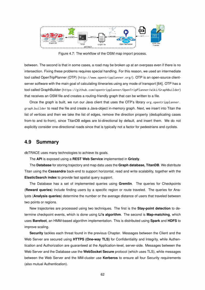
Figure 4.7: The workflow of the OSM map import process.

between. The second is that in some cases, a road may be broken up at an overpass even if there is no

intersection. Fixing these problems requires special handling. For this reason, we used an intermediate

tool called OpenTripPlanner (OTP) (http://www.opentripplanner.org/). OTP is an open-source client-

server software with the main goal of calculating itineraries using any mode of transport [64]. OTP has a

tool called GraphBuilder (https://github.com/opentripplanner/OpenTripPlanner/wiki/GraphBuilder)

that receives an OSM file and creates a routing-friendly graph that can be written to a file.

Once the graph is built, we run our Java client that uses the OTP’s library org.opentripplanner.

graph builder to read the file and create a Java-object in-memory graph. Next, we insert into Titan the

list of vertices and then we take the list of edges, remove the direction property (deduplicating cases

from-to and to-from), since TitanDB edges are bi-directional by default, and insert them. We do not

explicitly consider one-directional roads since that is typically not a factor for pedestrians and cyclists.

4.9 Summary

dbTRACE uses many technologies to achieve its goals.

The API is exposed using a REST Web Service implemented in Grizzly.

The Database for storing trajectory and map data uses the Graph database, TitanDB. We distribute

Titan using the Cassandra back-end to support horizontal, read and write scalability, together with the

ElasticSearch index to provide fast spatial query support.

The Database has a set of implemented queries using Gremlin. The queries for Checkpoints

(Reward queries) include finding users by a specific region or route traveled. The queries for Ana-

lysts (Analysis queries) determine the number or the average distance of users that traveled between

two points or regions.

New trajectories are processed using two techniques. The first is the Stay-point detection to de-

termine checkpoint events, which is done using Li’s algorithm. The second is Map-matching, which

uses Barefoot, an HMM-based algorithm implementation. This is distributed using Spark and HDFS to

improve scaling.

Security tackles each threat found in the previous Chapter. Messages between the Client and the

Web Server are secured using HTTPS (One-way TLS) for Confidentiality and Integrity, while Authen-

tication and Authorization are guaranteed at the Application-level, server-side. Messages between the

Web Server and the Database use the WebSocket Secure protocol (which uses TLS), while messages

between the Web Server and the MM-cluster use Kerberos to ensure all four Security requirements

(also mutual Authentication).

62

Visualization of the query results is done using a Javascript application using Leaflet. This allows

for easy integration into browser or mobile applications.

Finally, the importing of the road network into Titan is done using the Graphbuilder module of

OTP, accessing data from the OSM repository.

63

Chapter 5

Results

In the previous Chapter, we delved into the details of the technology solutions and algorithms used for

implementing dbTRACE. In this Chapter, we test and analyze the implemented system to determine if it

effectively achieves all the requirements of a solution to the problem introduced in Chapter 1.

We start in Section 5.1.1 (Index Performance) where we measure the effect of the each type of

index on Titan performance. Section 5.2 (Distributed Performance) tests query performance when

running in a multi-machine cluster as well as multi-client environment. In addition, two different config-

uration settings for the Cassandra storage back-end are compared to see its effect on performance. In

Section 5.3 (Database Query Analysis) we analyze the query running time in the graph database as

query complexity grows. Section 5.4 (Map Matching) discusses several aspects of the Map Matching

cluster. This includes the overall accuracy of the algorithm against the tested routes as well as the

single-machine performance as a function of trajectory size. In addition, we show the effect in running

time when using the Scala distributed framework. We end the chapter in Section 5.5 (Importing Map

Data) where we measure the import process run-time against a real use-case.

5.1 Index Performance

This test measures the response times of the different indexing options available to TitanDB in order to

determine the best index configurations to query spatial data.

The data-set we used was composed of 250 000 vertices with a coordinate location property, spread

out over Lisbon. In addition, we created a total of 250 trajectories with a total of 750000 edges. Each

trajectory had 3000 edges.

We performed these tests on a single machine with an Intel Core i5-4300U @ 1.90 Ghz processor,

4 GB memory and 128 GB SSD storage, using the BerkeleyDB storage back-end1.

1BerkeleyDB is a key-value database developed by Oracle and is one of the available storage back-ends for TitanDB.Reference: http://www.oracle.com/technetwork/database/database-technologies/berkeleydb/overview/index.html

64

5.1.1 Graph index

Graph indexes are global index structures over the entire graph. They allow the efficient retrieval of

vertices or edges by their properties on some specified condition.

Figure 5.1 shows a comparison of the spatial query response time for each graph index configuration,

as a function of the number of elements that the query returns in the answer set.

We evaluated the performance using the query: clockWithResult(10) {g.V().has(’location’,

geoWithin(area)).count().next();}, which gives us the number of points that are spatially contained

in the given area. We modified the area variable so that the size of the answer would return increasingly

more points.

Figure 5.1: A comparison of the response time in milliseconds (y axis) over the size of the answer set (xaxis) for the different TitanDB indexing options.

The first thing to notice is that the response time between having no index, versus using a composite

index gives the same results. Furthermore, the response time does not change with the answer set size.

That is, TitanDB does not use composite indexes for spatial queries, it instead relies on a full graph scan

to perform a spatial search.

To perform spatial queries efficiently, we require the use of an index back-end, i.e., Solr and Elastic-

Search. As can be seen in Figure 5.1, ElasticSearch gives strictly better results than Solr. Furthermore,

the response time varies linearly with the number of results in the answer set, potentially being slower

than a full graph scan when the answer set is too big. However, most queries will tend to return a more

constrained answer set.

5.1.2 Vertex-centric index

Vertex-centric indexes are local index structures built on each vertex. These indexes can help when

traversing vertices that have thousands of incident edges, which need to be retrieved and filtered to

match the conditions for traversal.

This evaluation measures the impact of vertex-centric indexes on query performance. We tested this

using the ElasticSearch index and the Average Trip Distance query (Listing 4.17). We chose this query

because its run-time is mostly edge-traversal, and thus, sees the most impact from this type of index.

65

The impact on the other queries is minimal.

Table 5.1: Comparing the performance of the query as a function of data-set size (percentage). Thesecond column indicates the response time in milliseconds when not using an index, while the thirdcolumn shows the results when using an index. The last column shows the improvement in running timewhen using the index.

Data-set size (%) w/o index (ms) w/ index (ms) gains (%)12.5 457 461 0.8825 1681 1467 14.5950 7271 5878 23.7100 21828 17432 25.22

From Table 5.1, we can see the improvement in query performance. However, this improvement only

becomes relevant when the data-set size increases beyond a certain point.

For the first row, with a data-set size of 31250 vertices and 93750 edges, the index setting does not

show any notable impact. From the second row onward however, we start to notice the improvement.

With a 25% data-set size, i.e., 62500 vertices and 187500 edges, we got a 14.59% improvement in

speed. As the data-sets became larger, the speed increase became constant, with both the 50% data-

set and the full data-set showing about 24% improvement (23.7% and 25.22%, respectively).

5.2 Distributed Performance

To test the performance of the database when used in a distributed fashion, we tested the system

response time as a function of the number of nodes, as well as a function of the number of concurrent

queries. We used Amazon Web Services (AWS) (http://aws.amazon.com/) to deploy a small Elastic

Compute Cloud (EC2)2 cluster.

For the instance type, we chose m4.large instances. The m4.large instances are general-purpose

machines with 2 vCPUs, running on a 2.4 GHz Intel Xeon E5-2676 processor and 8 GB memory. Cor-

bett3 gives an overview on picking an instance type for TitanDB on AWS, stating that the performance

of running a query (for example, shortest-path) only improves 9% when going from the m4.large to an

m4.2xlarge. We ran Cassandra and Gremlin-server on each of these machines that came bundled with

Titan 1.0. Each machine was also running an ElasticSearch (v1.5.2) node using the Transport Client

interface. Furthermore, we kept Cassandra’s consistency level (how many copies of the data item must

be read/written before a client sees the value) at one and the replication-factor (how many copies of

each data item exist) for both Cassandra and ES equal to the number of nodes until 3. Further added

nodes kept the replication-factor of 3.

The dataset was composed of 200 000 points (Lisbon has about 180 000 vertices) and 100 trajec-

tories, each with a length of 1000 edges (expected average trajectory size for a 1 hour run). All results

were measured using the profile().cap(TraversalMetrics.METRICS KEY) step operation.

2EC2 is the AWS service that allows launching virtual machines in one of Amazon’s data-centers.3Reference, http://blogs.aws.amazon.com/bigdata/post/Tx3JO46NGMX3WAW/Performance-Tuning-Your-Titan-Graph-

Database-on-AWS

66

5.2.1 Response Time

Titan has been shown to serve thousands of OnLine Transaction Processing (OLTP)4 requests per

second.5 However, many of the queries we use are OnLine Analytical Processing (OLAP)6-style analysis

queries.

Figure 5.2: Response time in milliseconds as a function of the number of nodes in the cluster. Sendingthe query to one of the machines in the cluster results in the Default line. The Parallel line shows amodified client that distributes the requested trajectories evenly between the nodes.

Figure 5.2 shows the run-time of an OLAP query as it goes from a single machine to an increasingly

distributed cluster of machines. We measured the response time in milliseconds for the Average trip

distance query (Section 4.4.2) in the default line, as well as a parallel version shown in the parallel line

described in the Appendix K.

Looking at the Default test, the first observation we can make is that the improvement in performance

is very small and linear as it goes from 1 node up to 3 nodes, with a total of approximately 8% improve-

ment at 3 nodes. When adding further nodes to the system, we stop seeing improvements in response

time. Second, it shows Titan does not distribute the workload of a single query on its own, processing

the 100 trajectories as a single traversal on 1 machine. The small improvement shown comes from the

increase in number of ElasticSearch nodes, which allows the spatial search to run in parallel on each

node.

We could get around this problem using Titan’s GraphComputer engine that allows OLAP computing,

sending the query to each vertex in the graph for parallel processing. However, at the time of writing

(Titan 1.0.0-release) the FulgoraGraphComputer7, which does not work in a distributed setting and the

GiraphGraphComputer, which only supports processing on graphs that fit in main memory, work correctly.

The SparkGraphComputer works on bigger graphs, but we did not get it to work due to several configura-

tion and documentation errors8. Support for the GiraphGraphComputer (Hadoop) is still planned but new

4OLTP queries refer to processing in which the system responds immediately to user requests (such as read, insert, updateand delete).

5Titan scaling, https://dzone.com/articles/titan-provides-real-time-big6OLAP, in contrast to OLTP, are characterized by much more complex queries designed for business intelligence or data

mining.7FulgoraGraphComputer is a single-machine, in-memory graph computer built for Titan.8Note: this is still true in Titan 1.1.0, but a branch of the repository has claimed to get it to work. However, we did not have

time to test it. Branch at: https://github.com/graben1437/titan1withtp3.1

67

updates have been slow.

However, we can still improve the response time by modifying the client to explicitly send each piece

of the query processing load to a different node in the cluster, as we explain in Appendix K. The first

observation with this modification (shown in the Parallel ’red’ line) is that there is a clear improvement

in response time as the number of nodes increase. Increasing the cluster from 1 node to 2 improves

the response time by 26%. The gains decrease as more nodes are added however, with the 4th to 5th

jump adding only an 8% improvement. We suspect that the added data partitioning and communication

overhead place a hard limit on scaling this kind of deep traversal queries.

Figure 5.3: The number of concurrent clients (1, 8 and 32) as a function of the number of nodes in thecluster, using the parallel Average Trip Distance query. For both the 8 and 32 series, the queries weresent at the same time and the time was measured when all results were returned.

Figure 5.3 shows the effect of the number of nodes as the number of concurrent users (using the

distribution-aware client) on the system increases.

As we can see, the run-time does not increase linearly with the number of users. Having 8 users as

opposed to 1 user increases the total run-time only by 50%. This is likely due to the caching mechanism

used by both Titan and ES, compounded by the fact that the trajectories were similar in most cases.

For both the 8 and 32 series, the improvements were more significant than the single user case, av-

eraging about 23.75% per added node. In particular, the largest improvement occurred when increasing

the number of nodes from 1 to 2 nodes, with 28.3% and 34.7%, respectively.

Another important aspect is that the response time did not increase linearly with the number of

concurrent requests. The reason for this is likely due to the number of cores available in the nodes as

well as Titan’s caching system.

The effect of adding extra nodes to the cluster does not significantly improve the run-time of deep

traversal queries. However, the greater benefit comes in system throughput, allowing more requests to

be issued concurrently to serve a greater number of clients.

5.2.2 Consistency Level

To test the impact of higher consistency levels on the system, we measured the response time to a full

graph scan for each of the different levels, shown in Figure 5.4. The figure shows the results for different

68

Figure 5.4: Response time in milliseconds as a function of the level of consistency in the Cassandracluster.

read consistency levels since writes always propagate to all replicas so the work done by the cluster is

the same when the consistency level is ONE or ALL. Our test setup was a cluster of 6 machines, with a

replication factor of 3. In these conditions, the consistency levels of ONE, QUORUM and ALL means we are

reading from one, two and three nodes, respectively.

As we can see from the figure, we see a 7% increase in latency when going from CL ONE to QUORUM.

This increase is likely the result of inter-node communication for consistency checks. However, going

from CL QUORUM to ALL shows less than a 1% increase in latency. We attribute this result to all the

nodes in our cluster having the same characteristics and the same load. In a real system with nodes

with different characteristics and different loads, the increase in latency would likely be bigger, since the

operation would depend on the slowest node to return the final result.

5.2.3 Replication Factor

Our final round of tests on distributed Titan was on the impact of the replication factor, i.e. the number of

replicas per data item, on query performance. For this test, we used 3 machines. Furthermore, we set

the read and write consistency level to 1.

Figure 5.5 shows our testing of the impact of the replication factor on read and write performance.

The x axis represents the replication factor, while the y axis indicates the elapsed time in milliseconds.

The red line shows the elapsed time to insert 100 000 vertices into the graph, while the blue line shows

the time to read 100 000 vertices from the graph.

Write performance worsens significantly with the number of replicas in the system. In our tests,

increasing the replication factor from 1 to 2 has an increase in response time of 21.83%, while from 2

to 3 the increase is 10.58% for a total of 34.71%. This is because every write to the cluster will end up

causing a write to every replica node for that data9.

Read performance on the other hand, receives a slight, more linear improvement. Increasing the

replication factor from 1 to 2 has an improvement of 6.86% in response time, while going from 2 to 3

9Reference, http://docs.datastax.com/en/cassandra/1.2/cassandra/architecture/architectureClientRequestsWrite.html

69

Figure 5.5: Response time in milliseconds as a function of the replication factor in the Cassandra cluster.

has an improvement of 6.55%, for a total of 12.96%. This improvement can be attributed to the fact that,

by increasing the replication factor, each node of the cluster will store more data, allowing the program

driver /coordinator more choice by reading from faster nodes and reading more data from the same

node, preventing more communication overhead10.

5.3 Database Query Analysis

This Section measures the run-time of the different implemented queries and analyzes their operations

to determine their respective bottlenecks. We performed this test on a machine using an Intel Core

i5-4200U 1.9 GHz processor with 4GB of RAM and 128 GB SSD storage.

We used BerkeleyDB for the storage database with a dataset of 180 000 vertices (approximate num-

ber of vertices in Lisbon). There were 100 trajectories (expected average number of filtered trajectories

measured in a query), with an average size of 547 edges (expected average size for a 30 minute trajec-

tory run).

The time was measured using the profile().cap(TraversalMetrics.METRICS KEY) operation. This

allows us to see each traversal step run-time, indicating the most expensive steps of the traversal, which

can be useful for optimization. However, this introduces severe overhead on the final run-time, usually 5

to 10 times more than the real result. These measurements are useful for a relative comparison between

objects, not as a performance benchmark.

Fig. 5.6 shows how the response time varies with query complexity. Calculating the number of users

that passed through a certain road is very quick, as expected. About 60% of the run-time is a graph

traversal from the beginning to the end of the road, while 30% is used on the deduplication of repeat

users and the final 10% is for the count-step.

The second query, which involves counting the number of users that started a trip in origin area and

ended the trip in destination area, we see a sharp increase in response time. There is first a spatial

filter operation (ES index look-up) that accounts for 5% of run-time. Each node has one edge traversal

and a filter operation (10%). For each filtered node, there is one spatial filter ES look-up, representing

10Reference, http://docs.datastax.com/en/cassandra/1.2/cassandra/architecture/architectureClientRequestsRead c.html

70

Figure 5.6: A comparison of the response time in milliseconds (y axis) between the different Analysisqueries (x axis).

85% of the run-time, which increases further as the filtering area increases and more nodes need ES

look-ups. This can likely be improved if we only do two spacial look-ups for finding the origin and destiny

sessions, and then finding the common elements in both sets using an algorithm such as the merge part

of the merge-sort algorithm.

Calculating the average distance of trips that start in origin area and end in destination area is

a good example of an expensive OLAP query, composed of a mix of the previous queries. First it has

a spatial filter operation to obtain the list of matching trajectories and then it has a traversal loop for

each of these trajectories (each will traverse 547 edges on average). For this particular data-set, the

spatial index look-up occupied about 30% of the run-time, while the traversal about 70%. However, this

disparity is likely to increase as the number of trajectories increase, with us showing in Section 5.1.1 that

the increase in the index response time increases very linearly with the number of items in the result

set. However, this does not occur with traversal time as the size of the trajectories increase, as can

be seen in the first data point of Figure 5.2 in the next Section, which has trajectories with double the

size but a 2 orders of magnitude greater run-time. This query can be easily optimized by adding the

trajectory distance to the session node as a simple attribute. This would reduce the query to just the

filtering operation, completely eliminating the traversal operation. However, for the purposes of further

load testing in the next sections, this query is used as a representative OLAP expensive traversal.

5.4 Map matching

The objective of this study is to evaluate the performance of the Map matching module in terms of:

accuracy, running time, distributed running time, and space savings. These tests were conducted by

running Barefoot using the configurations we defined in Section 4.5.3. Map data was for a region of

Portugal encompassing Lisbon, Sintra and Cascais, consisting of 236 961 ways.

We used 3 different trajectories as the input data set. The first was for a Sintra bicycle trip, shown

in Figure 5.7 encompassing 3081 longitude/latitude point pairs over the span of 3 hours, 30 minutes

and 30 seconds. Measurement period varied between 3 and 15 seconds (measurements were taken

71

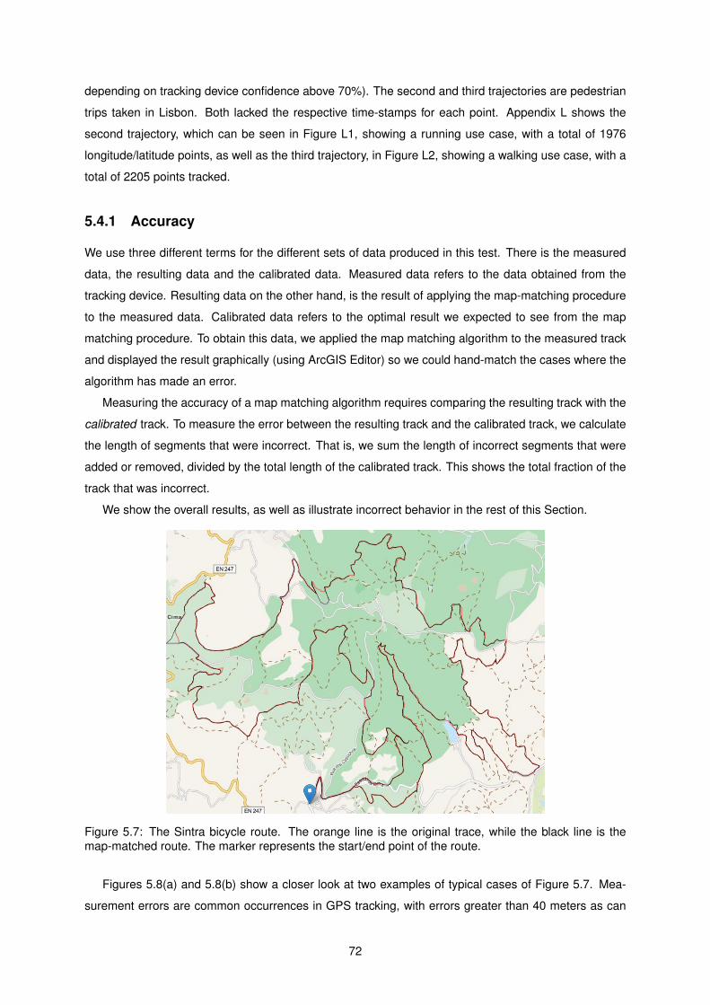
depending on tracking device confidence above 70%). The second and third trajectories are pedestrian

trips taken in Lisbon. Both lacked the respective time-stamps for each point. Appendix L shows the

second trajectory, which can be seen in Figure L1, showing a running use case, with a total of 1976

longitude/latitude points, as well as the third trajectory, in Figure L2, showing a walking use case, with a

total of 2205 points tracked.

5.4.1 Accuracy

We use three different terms for the different sets of data produced in this test. There is the measured

data, the resulting data and the calibrated data. Measured data refers to the data obtained from the

tracking device. Resulting data on the other hand, is the result of applying the map-matching procedure

to the measured data. Calibrated data refers to the optimal result we expected to see from the map

matching procedure. To obtain this data, we applied the map matching algorithm to the measured track

and displayed the result graphically (using ArcGIS Editor) so we could hand-match the cases where the

algorithm has made an error.

Measuring the accuracy of a map matching algorithm requires comparing the resulting track with the

calibrated track. To measure the error between the resulting track and the calibrated track, we calculate

the length of segments that were incorrect. That is, we sum the length of incorrect segments that were

added or removed, divided by the total length of the calibrated track. This shows the total fraction of the

track that was incorrect.

We show the overall results, as well as illustrate incorrect behavior in the rest of this Section.

Figure 5.7: The Sintra bicycle route. The orange line is the original trace, while the black line is themap-matched route. The marker represents the start/end point of the route.

Figures 5.8(a) and 5.8(b) show a closer look at two examples of typical cases of Figure 5.7. Mea-

surement errors are common occurrences in GPS tracking, with errors greater than 40 meters as can

72

be seen in 5.8(a). Furthermore, 5.8(b) shows the algorithm performing well in a situation with multiple

intersections, choosing the correct, most logical route, instead of the closest route.

(a) Example A (b) Example B

Figure 5.8: The map matching snapping effect. The orange line is the original trace, while the black lineis the map-matched route. The traced line beneath the black line is the actual path.

Figures 5.9(a) and 5.9(b) show what happens when the user takes a shortcut for which there is no

mapped road. In both cases, the possible paths, i.e., the long way around, exceeded the matcherMaxDistance

parameter, resulting in a break in the trajectory. In this case, it is the most desirable outcome, since there

is no actual underlying path in our road network data. This is helpful for urban planning purposes, since

it allows us to identify points where new shortcuts can be helpful.

(a) Example A (b) Example B

Figure 5.9: Map matching break on an incomplete path example. The breaks are shown as yellowcircles.

Figure 5.10 shows the opposite effect. The matcher incorrectly added segments of road to the

trajectory, showing the user going around the pavilion trying to find a possible route, instead of breaking

the trajectory. In this case, the possible path had under 234 m of length, which combined with the 15

m of position error allowed by matcherSigma, did not exceed the value we set for matcherMaxDistance,

leading to an incorrect matching.

Table 5.2 illustrates the results we obtained for each route and allows for a quick comparison of the

different cases.

For the first route the map-matching performed correctly with an average of 97%. In the second and

third routes the result was significantly worse with 83% and 90% respectively. This gives us an average

of 90%. Testing each different trajectory is time-consuming, leading to a small sample size. However,

we used a good representation of the different use cases, leading us to believe that these results will

73

Figure 5.10: An example of an incorrect segment addition as a result of a lenient matching process. Theuser took a shortcut through the pavilion, but since there is not a corresponding path in the map networkand the matcher candidate requirements were lowered to account for GPS errors, a round-about routewas found instead of breaking the trajectory.

Table 5.2: Comparing the accuracy for the three different tested routes. For each case, we indicate thelength of the calibrated trajectory, followed by the length of the incorrect segments of the resulting trackand the overall accuracy percentage according to the formula mentioned above.

Calibrated trajectory (m) Incorrect segments (m) Correct match %Bicycle route 40462 1561 97Running route 19326 3958 83Walking route 22763 2529 90

likely be seen in general. We attribute the degradation in the pedestrian routes to the tendency of users

to take more shortcuts, leading more often to cases depicted in Figure 5.10. Another factor to consider

is the state of the road network information. In some cases, the OSM map data may be incomplete or

may not correspond to the the state of the network when the trajectory was taken. The pedestrian routes

were taken in a city environment which changes much more quickly than the more rural roads of Sintra.

5.4.2 Running Time

We tested the performance of the Barefoot algorithm, running on a commodity server. The machine was

running an Ubuntu 14.04 version, with an Intel Core i3 CPU @ 3.07GHz and 4 GB of memory. The map

data was stored in a Docker container11 running a PostgreSQL/PostGIS database server.

Figure 5.11 shows the performance of the algorithm as a function of the size of the trajectory. This

relationship is strongly linear. The maximum value we obtain, for a trajectory with 3000 points, is a

running time of approximately 11 seconds. This running time is improved by the caching mechanism

11Docker is an Operating-system-level virtualization software. Programs in virtual partitions (typically called containers) use theoperating system’s normal system call interface and resources instead of being emulated by an intermediate virtual machine. LikeVM images, container images are a snapshot of a system state that can be later started and run. Website, https://www.docker.com

74

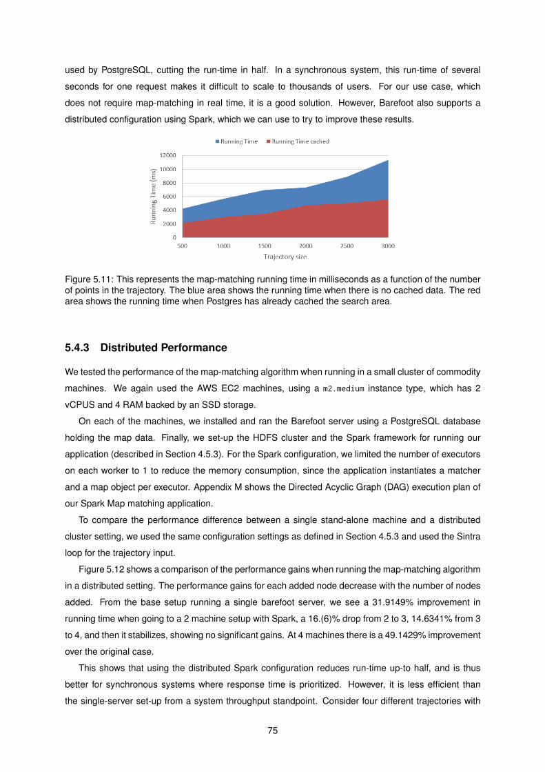
used by PostgreSQL, cutting the run-time in half. In a synchronous system, this run-time of several

seconds for one request makes it difficult to scale to thousands of users. For our use case, which

does not require map-matching in real time, it is a good solution. However, Barefoot also supports a

distributed configuration using Spark, which we can use to try to improve these results.

Figure 5.11: This represents the map-matching running time in milliseconds as a function of the numberof points in the trajectory. The blue area shows the running time when there is no cached data. The redarea shows the running time when Postgres has already cached the search area.

5.4.3 Distributed Performance

We tested the performance of the map-matching algorithm when running in a small cluster of commodity

machines. We again used the AWS EC2 machines, using a m2.medium instance type, which has 2

vCPUS and 4 RAM backed by an SSD storage.

On each of the machines, we installed and ran the Barefoot server using a PostgreSQL database

holding the map data. Finally, we set-up the HDFS cluster and the Spark framework for running our

application (described in Section 4.5.3). For the Spark configuration, we limited the number of executors

on each worker to 1 to reduce the memory consumption, since the application instantiates a matcher

and a map object per executor. Appendix M shows the Directed Acyclic Graph (DAG) execution plan of

our Spark Map matching application.

To compare the performance difference between a single stand-alone machine and a distributed

cluster setting, we used the same configuration settings as defined in Section 4.5.3 and used the Sintra

loop for the trajectory input.

Figure 5.12 shows a comparison of the performance gains when running the map-matching algorithm

in a distributed setting. The performance gains for each added node decrease with the number of nodes

added. From the base setup running a single barefoot server, we see a 31.9149% improvement in

running time when going to a 2 machine setup with Spark, a 16.(6)% drop from 2 to 3, 14.6341% from 3

to 4, and then it stabilizes, showing no significant gains. At 4 machines there is a 49.1429% improvement

over the original case.

This shows that using the distributed Spark configuration reduces run-time up-to half, and is thus

better for synchronous systems where response time is prioritized. However, it is less efficient than

the single-server set-up from a system throughput standpoint. Consider four different trajectories with

75

Figure 5.12: This chart provides a relative comparison of the running time in seconds in different compu-tation set-ups. The first bar on the left serves as a reference point, running the usual barefoot applicationon one machine. The following bars are running our Spark application, with the number reference indi-cating how many machines are in the cluster.

the same size as the Sintra track and four machines running a separate Barefoot server. The 4 tracks

will finish in 11 seconds. The distributed setting will finish each track in 5.7 seconds for a total of 22.8

seconds.

5.4.4 Space savings

Another benefit of map matching is the conversion of a series of time-stamped location points, to a series

of road identifiers. This allows us to reduce the size of the data in order to save space.

Table 5.3: Comparing the accuracy for the three different tested routes. For each route, we compare thenumber of vertices and edges in the original state, as well as the state after the Map-matching process.In addition, we also compare the storage space needed in MegaBytes.

Bicycle route Running route Walking routeOriginal V + E 3083 + 3082 1976 + 1975 2205 + 2204

After-MM V + E 0 + 3655 0 + 2194 0 + 2625Nr. Object savings % 40.7 44.8 40.5Original Space (MB) 3.28 2.10 2.34

After-MM Space (MB) 2.69 1.61 1.93Storage Savings % 18.0 23.3 17.5

Table 5.3 shows the impact of Map-matching on the amount of storage space that can be saved.

Each vertex consists of 2 properties. A String property name and a Geopoint property location. The

space occupied by each vertex was 290 Bytes. Each edge consists of 2 properties. A String property

session id and a Date property date. The space occupied by each edge was 735 Bytes.

Space is an important consideration in a system that needs to keep growing with the number of

users. Not only do we reduce on average 20% of storage space, but we also eliminate the additional

managing and indexing of objects in the system by an average of 42%.

76

5.5 Importing Map Data

This final test measures the total running time of the import process of OSM data. We analyze the

contribution of each part of the process, from the building of the in-memory road network graph by OTP,

to the insertion of the graph (both vertices and edges) into TitanDB.

We ran this test on a single machine with a 64-bit Intel Core i5-4300 processor, 4 GB of memory and

128 GB SSD, using the Cassandra back-end and ElasticSearch index.

The data-set was the road network of Lisbon, which at the time of writing (September 2016) has

|V | = 183130 and |E| = 484144.

Figure 5.13: The difference between the import time at run-time with Titan’s integrity checks on (Trans-actional) vs. integrity checks off (Batch-loading).

Figure 5.13 shows that running the import process during operational period, where transactional

and integrity measures are enforced, takes approximately 96 minutes (1 hour 36 minutes). A rate of

103.867 vertex insertions per second and 121.586 edge insertions per second. Disabling Titan’s internal

consistency and transactional checks (storage.batch-loading=true), makes the process much quicker,

taking about 16 minutes. This increases the rate to 960.797 vertex insertions per second and 677.122

edge insertions per second.

Another way to speed up the import process would be to use Titan’s OLAP-based graph processing

back-ends such as Hadoop or Spark to add all the vertexes in parallel followed by the edges. This

featured is not yet implemented as of time of writing.

5.6 Summary

This Chapter analyzed several components of dbTRACE. For the Database component, we tested the

different indexing options. We showed that global indexes are essential when doing geospatial searches

and that of all the options available, ElasticSearch was the clear winner. Vertex-centric indexes are

also important when doing traversals in large data-sets, leading to faster traversals as the data-set grows

larger (up to about 25% in our tests).

We distributed the Database using the Cassandra back-end and found that the run-time of a deep

traversal query (a query that goes from one node to another by traversing many edges) does not im-

prove significantly as more nodes are added, even when a query is composed of many separate

deep traversals. Titan dropped support for parallelizing traversal queries (used to be called the Titan-

MultiVertexQuery ) and has yet to implement distributed OLAP graph engines, which means we must

77

explicitly modify the client to parallelize the query. Once we do this, we find that the response time

improves logarithmically as the number of nodes increase, with an improvement of about 54% when

using 5 machines compared to the one machine case. The greatest benefit of adding more nodes

comes in system throughput. In an environment with 32 clients requesting heavy OLAP queries

(AvgTripDistance), we see gains of on average 24% per added node (again, lesser gains as more nodes

are added).

We analyzed the different queries developed and how they compare to each other in terms of run-

time. In addition, we determined the expensive operations of each query and recommended ways to

improve them.

We also analyzed Map-matching accuracy, run-time and space savings. We showed that for our

(small) test set, we obtained an average road matching accuracy of 90%. We also see gains in

performance when using a distributed environment. Using a Scala application with 4 machines we

saw gains in run-time for a single query of almost 48% compared to using one single machine.

However, if we want higher throughput, the Scala distributed map-matching is not efficient.

78

Chapter 6

Conclusion

This thesis addresses the design, implementation and evaluation of dbTRACE, a platform for storing

and managing spatial information generated by the TRACE users.

There is a scarcity of platforms for large-scale managing and storing of user tracking data. These

components must work together to build a solution that meets all the requirements of the TRACE initia-

tive. These requirements encompass: support for large-scale data storage and mining, reliability

and security. In addition, all interactions, as well as the location data itself is exchanged/stored while

ensuring the end-users’ privacy.

We developed a representative range of queries using the Gremlin language that enables urban

planning data-mining and reward validation. Scalable storage is achieved through the Cassandra dis-

tributed database for a master-master, no single-point-of-failure storage using commodity hardware.

Reliability is obtained using distributed transactions and replication supported by the TitanDB a graph

engine. Scalable query performance is achieved through an ElasticSearch cluster, providing sup-

port for spatial query capabilities. As of the moment of writing (Titan release 1.0.0), OLAP-based graph

analytics do not work properly in a distributed setting. There have been recent updates (Titan 1.1.0-

snapshot) that have fixed some of the bugs but there is still no ETA on an official release. Unfortunately,

we did not use these versions but it would be interesting to test them in the future.

To support the effective storage and querying of trajectory information, we pre-process the

information using two techniques. First, we use a Stay-point detection process to identify points where

the user likely spent some time. This is important for finding which checkpoints the user stayed at for

reward validation. Second, we use a Map-matching process using Barefoot, a Java library that uses

Newson and Krumm’s HMM algorithm for accurate results and Apache Spark for scalable performance.

This is important for quicker query analysis and lowering the space footprint.

The interface to the system uses a simple REST API provided by the Grizzly Web Server which

incorporates NIO-based stream handling in order to service many clients at the same time.

In order to visualize and test our application, we developed a small browser/mobile map interface

through the use of Leaflet.

In order to protect user privacy, we guarantee that all communication to and between the system

79

meets the four main security requirements, i.e., Confidentiality, Integrity, Authentication and Authoriza-

tion. Messages between the components in the system are passed using secure layers 2-way authen-

tication layers, while messages between the client and the front-end server use server-authentication

and provides a password-based client authentication at application level.

We discuss the limitations and the possible improvements and openings for further research resulting

from this work in Section 6.

Future Work

During the time that we worked on this topic, we were able to identify several possible future contributions

to this area. We conclude this document with the following ideas for future work:

• Implement level 2 and 3 planner queries: We implemented the highest priority queries according

to the level of importance attributed by the partners, shown in Appendix B. Due to time constraints,

we were unable to implement all requested queries. This addition would lead to an increase in

usefulness of the platform.

• Improve the route comparison algorithm: We used the LCS algorithm for solving the route

comparison problem, which has O(mn) space and time complexity. However, there are better

options. Vlachos et al. [60] analyze this problem in more depth and offer a solution that also takes

into account trajectory noise for more robust result matching. In addition, Hunt and Szymanski [65]

developed an algorithm with a worst case asymptotic run-time O((n +m) ∗ log(n)) and best case

O(n ∗ log(n)).

• Integrated Map matching: We implemented map-matching using Barefoot, a Map-matching

client-server software that uses a relational database to host the road network. However, we could

remove this dependency by writing the HMM map-matching algorithm in Gremlin and using it di-

rectly with the data in the Titan database, which we expect would lead to significant performance

improvements.

• Fraud measures: Before any of the pre-processing steps are performed, trajectories need to be

verified for potential fraud occurrences. In this document, we detailed (in the Architecture Section)

the different fraud counter-measures needed for this project, but did not implement them. This step

can be easily integrated in the Pre-processing cluster for example.

• Incremental Map Import: According to TomTom, road networks change by as much as 15% each

year1. As such, map data must be updated periodically. OSM has OsmChange files that indicate all

the create/modify/delete actions that occurred between two OSM files. These files can be obtained

from using the osmconvert tool (osmconvert old.osm new.osm --diff -o=changefile.osc). This

file can then be easily parsed (XML format) to insert the changes into the database. Particular care

must be taken with modifications and deletions, since trajectory data may already be assigned. The

previous values would probably be kept for historical and analysis purposes.

1http://annualreport2015.tomtom.com/docs/TomTom2015/index.php?nr=160&r code=TomTom2015

80

Bibliography

[1] P. C. Arden Pope III, P. Richard T. Burnett, M. Michael J. Thun, P. Eugenia E. Calle,

P. Daniel Krewski, P. Kazuhiko Ito, and S. George D. Thurston. Lung cancer, cardiopulmonary

mortality, and long-term exposure to fine particulate air pollution. Journal of American Medical

Association, 2002.

[2] M. Martine S. Bernstein, P. Alfredo Morabia, MD, and M. Dorith Sloutskis. Definition and Prevalence

of Sedentarism in an Urban Population. American Journal of Public Health, 1999.

[3] M. Hilbert and P. Lopez. The world’s technological capacity to store, communicate, and compute

information. science, 332(6025):60–65, 2011.

[4] F. Giannotti and D. Pedreschi. Mobility, data mining and privacy: Geographic knowledge discovery.

Springer Science & Business Media, 2008.

[5] P. Amirian, A. Basiri, and A. Winstanley. Evaluation of data management systems for geospatial big

data. In International Conference on Computational Science and Its Applications, pages 678–690.

Springer, 2014.

[6] M. Michael, J. E. Moreira, D. Shiloach, and R. W. Wisniewski. Scale-up x scale-out: A case study

using nutch/lucene. In Parallel and Distributed Processing Symposium, 2007. IPDPS 2007. IEEE

International, pages 1–8.

[7] C. de Souza Baptista, C. E. S. Pires, D. F. B. Leite, and M. G. de Oliveiraa. NoSQL Geographic

Databases: An Overview. Geographical Information Systems: Trends and Technologies, page 73,

2014.

[8] D. Pritchett. Base: An ACID alternative. Queue, 6(3):48–55, 2008.

[9] R. Cattell. Scalable SQL and NoSQL data stores. ACM SIGMOD Record, 39(4):12–27, 2011.

[10] O. G. Consortium et al. OpenGIS® Implementation Specification for Geographic information-Simple

feature access-Part 1: Common architecture. OGC document, 2011.

[11] C. ISO. 19125-1. Geographic Information—Simple Feature Access—Part, 1.

[12] M. Barthelemy. Spatial networks. Physics Reports 499:1-101, 2011.

81

[13] V. Kanjilal and M. Schneider. Spatial network modeling for databases. In Proceedings of the 2011

ACM Symposium on Applied Computing, pages 827–832. ACM, 2011.

[14] R. H. Guting. An introduction to spatial database systems. The VLDB Journal—The International

Journal on Very Large Data Bases, 3(4):357–399, 1994.

[15] J. Weinberger. The spatial RDBMS in the Enterprise. Directions Magazine, 2002.

[16] S. Spaccapietra, C. Parent, M. L. Damiani, J. A. de Macedo, F. Porto, and C. Vangenot. A concep-

tual view on trajectories. Data & knowledge engineering, 65(1):126–146, 2008.

[17] Y. Zheng. Trajectory Data Mining: An Overview. ACM Transaction on Intelligent Systems and

Technology, September 2015. URL http://research.microsoft.com/apps/pubs/default.aspx?

id=241453.

[18] Y. Zheng, L. Zhang, X. Xie, and W.-Y. Ma. Mining interesting locations and travel sequences from

gps trajectories. In Proceedings of the 18th International Conference on World Wide Web, pages

791–800. ACM, 2009.

[19] Y. Zheng. Trajectory data mining: An Overview. ACM Transactions on Intelligent Systems and

Technology (TIST), 6(3):29, 2015.

[20] W.-C. Lee and J. Krumm. Trajectory preprocessing. In Computing with spatial trajectories, pages

3–33. Springer, 2011.

[21] Q. Li, Y. Zheng, X. Xie, Y. Chen, W. Liu, and W.-Y. Ma. Mining user similarity based on location

history. In Proceedings of the 16th ACM SIGSPATIAL international conference on Advances in

geographic information systems, page 34. ACM, 2008.

[22] N. J. Yuan, Y. Zheng, L. Zhang, and X. Xie. T-finder: A recommender system for finding passengers

and vacant taxis. IEEE Transactions on Knowledge and Data Engineering, 25(10):2390–2403,

2013.

[23] D. H. Douglas and T. K. Peucker. Algorithms for the reduction of the number of points required to

represent a digitized line or its caricature. Cartographica: The International Journal for Geographic

Information and Geovisualization, 10(2):112–122, 1973.

[24] J. E. Hershberger and J. Snoeyink. Speeding up the Douglas-Peucker line-simplification algorithm.

University of British Columbia, Department of Computer Science, 1992.

[25] M. Potamias, K. Patroumpas, and T. Sellis. Sampling trajectory streams with spatiotemporal criteria.

In Scientific and Statistical Database Management, 2006. 18th International Conference on, pages

275–284.

[26] Y. Zheng, L. Liu, L. Wang, and X. Xie. Learning transportation mode from raw gps data for ge-

ographic applications on the web. In Proceedings of the 17th International Conference on World

Wide Web, pages 247–256. ACM, 2008.

82

[27] M. A. Quddus, W. Y. Ochieng, and R. B. Noland. Current map-matching algorithms for trans-

port applications: State-of-the art and future research directions. Transportation Research Part C:

Emerging Technologies, 15(5):312–328, 2007.

[28] F. Marchal, J. Hackney, and K. Axhausen. Efficient map matching of large global positioning sys-

tem data sets: Tests on speed-monitoring experiment in Zurich. Transportation Research Record:

Journal of the Transportation Research Board, (1935):93–100, 2005.

[29] W. Y. Ochieng, M. A. Quddus, and R. B. Noland. Map-matching in complex urban road networks.

Brazilian Society of Cartography, Geodesy, Photogrammetry and Remote Sensing (SBC), 2003.

[30] P. Newson and J. Krumm. Hidden Markov map matching through noise and sparseness. In Pro-

ceedings of the 17th ACM SIGSPATIAL international conference on advances in geographic infor-

mation systems, pages 336–343. ACM, 2009.

[31] F. C. Pereira, H. Costa, and N. M. Pereira. An off-line map-matching algorithm for incomplete map

databases. European Transport Research Review, 1(3):107–124, 2009.

[32] E. Bertino and R. Sandhu. Database security-concepts, approaches, and challenges. IEEE Trans-

actions on Dependable and Secure Computing, 2005.

[33] M. E. Whitman. Enemy at the gate: threats to information security. Communications of the ACM,

46(8):91–95, 2003.

[34] S. Myagmar, A. J. Lee, and W. Yurcik. Threat modeling as a basis for security requirements. In

Symposium on requirements engineering for information security (SREIS), volume 2005, pages

1–8, 2005.

[35] T. N. Phan, T. K. Dang, and J. Kung. User privacy protection from trajectory perspective in location-

based applications. Proc. of the 19th Interdisciplinary Information Management Talks, Jindichv

Hradec, Czech Republic, pages 281–288, 2011.

[36] C.-Y. Chow and M. F. Mokbel. Trajectory privacy in location-based services and data publication.

ACM SIGKDD Explorations Newsletter, 13(1):19–29, 2011.

[37] L. Sweeney. k-anonymity: A model for protecting privacy. International Journal of Uncertainty,

Fuzziness and Knowledge-Based Systems, 10(05):557–570, 2002.

[38] J.-G. Lee, J. Han, and X. Li. Trajectory outlier detection: A partition-and-detect framework. In Data

Engineering, 2008. ICDE 2008. IEEE 24th International Conference on, pages 140–149. IEEE,

2008.

[39] W. He, X. Liu, and M. Ren. Location cheating: A security challenge to location-based social network

services. In Distributed computing systems (ICDCS), 2011 31st International Conference on, pages

740–749. IEEE, 2011.

83

[40] B. Carbunar and R. Potharaju. You unlocked the Mt. Everest badge on foursquare! Countering

location fraud in geosocial networks. In Mobile Adhoc and Sensor Systems (MASS), 2012 IEEE

9th International Conference on, pages 182–190. IEEE, 2012.

[41] S. Saroiu and A. Wolman. Enabling new mobile applications with location proofs. In Proceedings

of the 10th workshop on Mobile Computing Systems and Applications, page 3. ACM, 2009.

[42] E. F. Codd. A relational model of data for large shared data banks. Communications of the ACM,

13(6):377–387, 1970.

[43] W. Kresse and D. M. Danko. Springer handbook of geographic information. Springer Science &

Business Media, 2012.

[44] A. Aitchison and J. Horner. Pro Spatial with SQL Server 2012. Springer, 2012.

[45] G. Weglarz. Two Worlds Data-Unstructured and Structured. DM REVIEW, 14:19–23, 2004.

[46] L. Hsu and R. Obe. Cross compare of SQL server, MySQL, and PostgreSQL. Postgres OnLine

Journal, 2008.

[47] K. M. Benchmarking database performance for genomic data. J Cell Biochem, 2015.

[48] N. Leavitt. Will NoSQL databases live up to their promise? Computer, 43(2):12–14, 2010.

[49] K. Stolze. SQL/MM Spatial-The Standard to Manage Spatial Data in a Relational Database System.

In BTW, volume 2003, pages 247–264, 2003.

[50] S. Sharma, U. S. Tim, S. Gadia, R. Shandilya, and S. Peddoju. Classification and Comparison of

NoSQL Big Data Models.

[51] C. A. BARON. Nosql key-value dbs riak and redis.

[52] J. C. Anderson, J. Lehnardt, and N. Slater. CouchDB: the definitive guide. ” O’Reilly Media, Inc.”,

2010.

[53] D. B. West et al. Introduction to graph theory, volume 2. Prentice hall Upper Saddle River, 2001.

[54] A. M. de Sousa Nunes Marques Pinto. Promoting urban bicycle use through next-generatio cycle

track-and-score systems. Master’s thesis.

[55] S. Reddy, M. Mun, J. Burke, D. Estrin, M. Hansen, and M. Srivastava. Using mobile phones to

determine transportation modes. ACM Transactions on Sensor Networks (TOSN), 6(2):13, 2010.

[56] D. Luxen and C. Vetter. Real-time routing with OpenStreetMap data. In Proceedings of the 19th

ACM SIGSPATIAL International Conference on Advances in Geographic Information Systems, GIS

’11, pages 513–516, New York, NY, USA, 2011. ACM. ISBN 978-1-4503-1031-4. doi: 10.1145/

2093973.2094062. URL http://doi.acm.org/10.1145/2093973.2094062.

84

[57] S. Mattheis, K. K. Al-Zahid, B. Engelmann, A. Hildisch, S. Holder, O. Lazarevych, D. Mohr,

F. Sedlmeier, and R. Zinck. Putting the car on the map: A scalable map matching system for

the Open Source Community. In GI-Jahrestagung, pages 2109–2119, 2014.

[58] G. DeCandia, D. Hastorun, M. Jampani, G. Kakulapati, A. Lakshman, A. Pilchin, S. Sivasubrama-

nian, P. Vosshall, and W. Vogels. Dynamo: amazon’s highly available key-value store. In ACM

SIGOPS Operating Systems Review, volume 41, pages 205–220. ACM, 2007.

[59] M. A. Rodriguez. The Gremlin graph traversal machine and language. In Proceedings of the 15th

Symposium on Database Programming Languages, pages 1–10. ACM, 2015.

[60] M. Vlachos, G. Kollios, and D. Gunopulos. Discovering similar multidimensional trajectories. In

Data Engineering, 2002. Proceedings. 18th International Conference on, pages 673–684. IEEE,

2002.

[61] D. S. Hirschberg. A linear space algorithm for computing maximal common subsequences. Com-

munications of the ACM, 18(6):341–343, 1975.

[62] P. A. Zandbergen and S. J. Barbeau. Positional accuracy of assisted GPS data from high-sensitivity

GPS-enabled mobile phones. Journal of Navigation, 64(03):381–399, 2011.

[63] A. Biryukov, D. Dinu, and D. Khovratovich. Fast and Tradeoff-Resilient Memory-Hard Functions for

Cryptocurrencies and Password Hashing. IACR Cryptology ePrint Archive, 2015:430, 2015.

[64] E. L. Hillsman and S. J. Barbeau. Enabling cost-effective multimodal trip planners through open

transit data. Technical report, 2011.

[65] J. W. Hunt and T. G. Szymanski. A fast algorithm for computing Longest Common Subsequences.

Communications of the ACM, 20(5):350–353, 1977.

85

Appendices

A The NoSQL Family

Figure A1: A visual mapping of the different SQL families (Sankar 2010).

86

B Urban planner indicators

Figure B1: Outline of the different indicators for urban planning and the level of importance and priorityattached. (Bernardino et al. 2016).

87

C Grizzly NIO Handler Implementation

Listing 1: The implementation of the non-blocking IO handler used for each service. onDataAvailable()

is called each time the client sends data to the server until the message is complete. When this hap-

pens, onAllDataRead() is called which sends the message to the calling handler function which will

verify the message and conditionally send it to the DBClient to transmit it to the database. Upon the

DBClient receiving the response back from the database, sendResponse() is called, finally transmitting

the response back to the requester.1 public class TraceNIOHandler extends ReadHandler {2 NIOReader in; NIOWriter out; Response response; APIHandler handler;3 final char[] buf = new char[128];4 final StringBuilder requestBuilder = new StringBuilder();56 public TraceNIOHandler(NIOReader in, NIOWriter out, Response response, APIHandler handler) { /* ... */ }78 @Override9 public void onDataAvailable() throws Exception {

10 requestBuilder.append(new String(buf));11 in.notifyAvailable(this);12 }13 @Override14 public void onAllDataRead() throws Exception {15 handler.callback(result.toString());16 }1718 public void sendResponse(String result) {19 try {20 out.write(result, 0, result.size());21 } catch(Exception e) {22 final String errorMsg = e.toString();23 Logger.log(Level.WARNING, errorMsg, e);24 out.write(errorMsg, 0, errorMsg.size()); // send error to client25 } finally {26 try { in.close(); } catch (IOException ioe) { LOGGER.log(Level.SEVERE, ioe.toString(), ioe); }27 try { out.close(); } catch (IOException ioe) { LOGGER.log(Level.SEVERE, ioe.toString(), ioe); }28 response.resume(); // call the service method to finalize the communication29 }30 }31 }

88

D LCS Implementation

Listing 2: Groovy adaptation of the LCS dynamic programming algorithm with asymptotic time O(mn)

and space O(n+m)

1 lcs length = { def A, def B −>2 if(A.size() < B.size()) { /* switch A and B in case B is larger */3 C = A; A = B; B = C;4 }5 def m = A.size();6 def n = B.size();7 def X = new int[ m + 1 ];8 def Y = new int[ n + 1 ];9 for (i = m−1; i >= 0; i−−) {

10 for (j = n−1; j >= 0; j−−) {11 if (i > m−1 || j > n−1)12 X[j] = 0;13 else if (A[i].equals(B[j]))14 X[j] = 1 + Y[j+1];15 else16 X[j] = Math.max(Y[j], X[j+1]);17 };18 for(k = 0; k < n; k++)19 Y[k] = X[k];20 };21 return X[0];22 };

89

E Stay-point Detection

Listing 3: Stay-point detection implementation written in Java1 public class StayPointDetection {2 private static final long DISTANCE THRESHOLD = 50L; // meters3 private static final long TIME THRESHOLD = 800000L; // milliseconds -> 8 minutes45 public List<StayPoint> getStayPoints(List<Point> trajectory) {6 List<StayPoint> stayPoints = new ArrayList<StayPoint>();7 int nPoints = trajectory.size();8 int i = 0;9 int j = 0;

10 while(i < nPoints) {11 j = i + 1;12 while(j < nPoints) {13 Point p1 = trajectory.get(i);14 Point p2 = trajectory.get(j);15 double dist = p1.distance(p2);16 if(dist > DISTANCE THRESHOLD) {17 long timeDiff = p2.getTime() − p1.getTime();18 if(timeDiff > TIME THRESHOLD) {19 float longitude = (p1.getLon() + p2.getLon()) / 2;20 float latitude = (p1.getLat() + p2.getLat()) / 2;21 long arrival = p1.getTime();22 long departure = p2.getTime();23 StayPoint newStayPoint = new StayPoint(longitude, latitude, arrival, departure);24 stayPoints.add(newStayPoint);25 }26 i = j; break;27 }28 j++;29 }30 return stayPoints;31 }32 }

90

F Grizzly Access Control

Listing 4: Authentication implementation using Grizzly1 static HttpServer createHttpServer(String url) throws IOException {2 server.getServerConfiguration().getMonitoringConfig().getWebServerConfig().addProbes(3 new HttpServerProbe.Adapter() {4 @Override5 public void onRequestReceiveEvent(HttpServerFilter filter, Connection connection, Request request) {6 final String user = request.getHeader("user");7 final String requestedOp = filter.getHttpHandler().getName();8 // perform authentication9 final Credentials creds = GrizzlyServer.credentialsDB.get(user);

10 if(creds == null) {11 connection.terminateWithReason(new InvalidUserException(user)); return;12 }13 // check if user already has valid session14 final String cookie = request.getCookies().iterator().next().getValue();15 LocalDateTime cookieExpiration = GrizzlyServer.cookieCache.get(cookie);16 if(cookieExpiration != null) {17 final boolean isCookieValid = LocalDateTime.now().isAfter(cookieExpiration);18 if(isCookieValid) {19 if(isAuthorized(requestedOp, creds.getRole())) { // check authorization20 return; // let the request go through21 } else {22 connection.terminateWithReason(new UnauthorizedException(user));23 return;24 }25 } else {26 request.clearCookies();27 }28 }29 // no valid session found, check if secret is valid30 GrizzlyServer.cookieCache.remove(user);31 if(isSecretValid(request, creds) && isAuthorized(requestedOp, creds.getRole())) { // authorization32 return; // let the request go through33 } else {34 connection.terminateWithReason(new UnauthorizedException(user));35 }36 }37 @Override38 public void onRequestCompleteEvent(HttpServerFilter filter, Connection connection, Response response) {39 if(response.getRequest().getNote("createNewCookie") != null) {40 final LocalDateTime cookieExpiration = LocalDateTime.now().plusMinutes(10);41 final SecureRandom random = new SecureRandom();42 final byte cookie[] = new byte[GrizzlyServer.COOKIE SIZE];43 random.nextBytes(cookie);44 GrizzlyServer.cookieCache.put(cookie, cookieExpiration);45 request.addCookie(new Cookie("cookie", new String(cookie)));46 }}});47 }

91

G Kerberized HDFS Client

Listing 5: The Kerberos HDFS client for the Web Server, written in Java.1 public void createFile(final String hdfsURL, final String trajectory) throws Exception {2 final Configuration conf = new Configuration();3 conf.set("fs.defaultFS", hdfsURL);4 conf.set("hadoop.security.authentication", "kerberos");5 conf.set("fs.hdfs.impl", org.apache.hadoop.hdfs.DistributedFileSystem.class.getName());6 final UserGroupInformation ugi = UserGroupInformation.loginUserFromKeytabAndReturnUGI(7 "webserver@HDFS.TRACE.ORG",8 "/etc/security/keytab/webserver.keytab");9 UserGroupInformation.setConfiguration(conf);

1011 ugi.doAs(new PrivilegedExceptionAction<Void>() {12 public Void run() throws Exception {13 final FileSystem fs = FileSystem.get(URI.create(hdfsURL), conf);14 final String fileName = new BigInteger(130, random).toString(32) + ".csv";15 final Path file = new Path(fileName);16 final BufferedWriter br = new BufferedWriter(new OutputStreamWriter(fs.create(file, true)));17 br.write(trajectory);18 br.close();19 return null;20 }});21 }

92

H Leaflet code

Listing 6: Javascript snippet showing our test visualization application using Leaflet1 var map = L.map(’map’).setView([38.70695, −9.13513], 9); // centering Lisbon2 L.tileLayer(’http://{s}.tile.osm.org/{z}/{x}/{y}.png’, {3 attribution: ’&copy; <a href="http://osm.org/copyright">OpenStreetMap</a> contributors’4 }).addTo(map);56 queryBox = L.control({position: ’topright’});7 queryBox.onAdd = function(map) {8 this. div = L.DomUtil.create(’div’, ’queryBox’);9 this. div.innerHTML = ’<input type="text" id="query" placeholder="Query..." ’

10 +’onkeydown="if(event.keyCode == 13){sendQuery(document.getElementById(\’query\’).value);}"/>’;11 return this. div;12 }13 queryBox.addTo(map);1415 function sendQuery(query) {16 var endpoint = webserverAddress;17 (isRouteID(query) || query == ’’) ? endpoint += ’/test’ : endpoint += ’/sendQuery’;18 httpGetAsync(endpoint, query, parseOutputCallback);19 }2021 function isRouteID(query) { // match anything except gremlin queries (strings with . and ())22 var pattern = /ˆ[ˆ().]+$/g;23 return pattern.test(query);24 }2526 function httpGetAsync(url, body, callback) {27 var client = new XMLHttpRequest();28 client.onreadystatechange = function() {29 if (client.readyState == 4 && client.status == 200)30 callback(client.responseText);31 }32 client.open("POST", url, true);33 client.setRequestHeader(’user’, "<user>");34 client.setRequestHeader(’secret’, hashFunction("<secret>"));35 client.setRequestHeader("Content-type", "application/x-www-form-urlencoded");36 client.send(body);37 }3839 function parseOutputCallback(data) {40 var results = JSON.parse(data);41 var keys = results[0].keys;42 if(keys.contains(’latitude’)) { // if it is a trajectory43 parseTrajectory(results);44 } else {45 alert(results);46 }47 }4849 function parseTrajectory(results) {50 var trajectory = []51 for(var i = 0; i < parsedArray.length; i++) {52 var point = [parsedArray[i].latitude, parsedArray[i].longitude];53 trajectory[i] = point;54 }55 // add trajectory to map56 if(parsedArray.length > 0) {57 var line = L.polyline(trajectory, {color: "#ff3030", weight: 2, opacity: 0.55}).addTo(map);58 }59 }

93

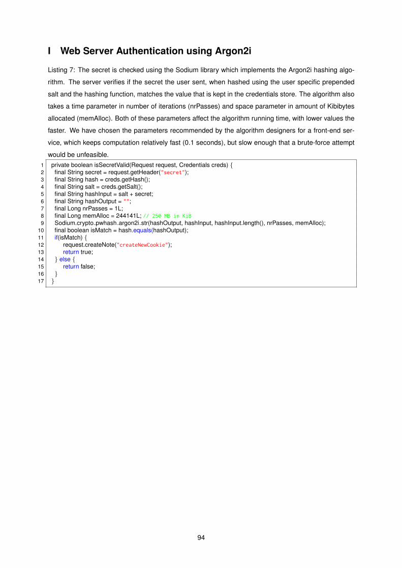
I Web Server Authentication using Argon2i

Listing 7: The secret is checked using the Sodium library which implements the Argon2i hashing algo-

rithm. The server verifies if the secret the user sent, when hashed using the user specific prepended

salt and the hashing function, matches the value that is kept in the credentials store. The algorithm also

takes a time parameter in number of iterations (nrPasses) and space parameter in amount of Kibibytes

allocated (memAlloc). Both of these parameters affect the algorithm running time, with lower values the

faster. We have chosen the parameters recommended by the algorithm designers for a front-end ser-

vice, which keeps computation relatively fast (0.1 seconds), but slow enough that a brute-force attempt

would be unfeasible.1 private boolean isSecretValid(Request request, Credentials creds) {2 final String secret = request.getHeader("secret");3 final String hash = creds.getHash();4 final String salt = creds.getSalt();5 final String hashInput = salt + secret;6 final String hashOutput = "";7 final Long nrPasses = 1L;8 final Long memAlloc = 244141L; // 250 MB in KiB9 Sodium.crypto pwhash argon2i str(hashOutput, hashInput, hashInput.length(), nrPasses, memAlloc);

10 final boolean isMatch = hash.equals(hashOutput);11 if(isMatch) {12 request.createNote("createNewCookie");13 return true;14 } else {15 return false;16 }17 }

94

J SSL Keystore and Truststore Configuration

Listing 8: The SSL configuration for the HTTP HDFS server endpoints, file 〈hadoop dir〉/conf/ssl-

server.xml

1 <configuration>2 <!−− Server Certificate Store −−>3 <property>4 <name>ssl.server.keystore.type</name>5 <value>jks</value>6 </property>78 <property>9 <name>ssl.server.keystore.location</name>

10 <value>${user.home}/keystores/server−keystore.jks</value>11 </property>1213 <property>14 <name>ssl.server.keystore.password</name>15 <value>keystore password</value>16 </property>1718 <!−− Server Trust Store −−>19 <property>20 <name>ssl.server.truststore.type</name>21 <value>jks</value>22 </property>2324 <property>25 <name>ssl.server.truststore.location</name>26 <value>${user.home}/keystores/truststore.jks</value>27 </property>2829 <property>30 <name>ssl.server.truststore.password</name>31 <value>truststore password</value>32 </property>3334 <property>35 </configuration>

95

K Parallel Average Trip Distance Query

Listing 9: The client-side parallel version of the Average Trip Distance Query. The query is split into two.

First the client fetches the sessions for the trajectories that will be processed. Then the session input

is partitioned and sent equally between the nodes in the cluster. When all results return, the mean is

calculated client-side and returned.1 public class DBClient {2 public void parallelAvgTripDistance(Region origin, Region destination, TRACENIOHandler ioHandler) {3 String getSessionsQuery = "g.V().has(’location’, geoWithin(origin))" +4 + ".inE(’session’).has(’type’, ’start’).outV()" +5 + ".inE(’session’).has(’type’, ’finish’).outV()" +6 + ".has(’location’, geoWithin(destination)).outE(’session’).has(’type’, ’finish’)" +7 + ".inV().value(’sessionID’)";8 Map<String,Object> params = new HashMap<>();9 params.put("origin", origin.toString()); // e.g. Geoshape.circle(-9.133920, 38.737047, 20)

10 params.put("destination", destination.toString());1112 List<String> results = null;13 try {14 // first get the sessions15 CompletableFuture<List<Result>> resultSet = client.submit(getSessionsQuery, params).all();16 results = resultSet.get().forEach( (Result r) −> results.add(r.toString()) );1718 // partition the sessions19 final double resultSize = results.size();20 final double clusterSize = client.cluster.availableHosts().size();21 final int partitionSize = Math.ceiling(resultSize / clusterSize);22 List<List<String>> partitions = new ArrayList<List<String>>();23 for (int i = 0; i < resultSize; i += partitionSize) {24 partitions.add(results.subList(i, Math.min(i + partitionSize, resultSize)));25 }2627 // for each partition, send a query to a different node28 String avgTripDistanceQuery = "g.withSack(’’).V(sessionList)" +29 + ".sack{m,v -> v.value(’sessionID’)}.repeat(outE().filter(filterEdgeBySession).inV())" +30 + ".until(hasLabel(’session’)).path().by(’location’).by(constant(’edge’))" +31 + ".map(calculateTripDistance).map({it.get().get()}).mean();";3233 List<CompletableFuture<ResultSet> avgTripDistanceResults = new ArrayList<>();34 for(List<String> partition : partitions) {35 String sessionInput = StringUtils.join(partition, ",");36 CompletableFuture<ResultSet> future = client.submitAsync(avgTripDistanceQuery, sessionInput);37 avgTripDistanceResults.add(future);38 }3940 // when all of them return, calculate mean41 CompletableFuture.allOf(avgTripDistanceResults).join();4243 Double meanDistance = new Double(0.0);44 for(CompletableFuture<ResultSet> f : avgTripDistanceResults) {45 meanDistance += f.all().get().get(0).getDouble();46 }47 meanDistance /= avgTripDistanceResults.size();48 ioHandler.sendResponse(meanDistance.toString());4950 } catch (Exception e) {51 LOGGER.log(Level.SEVERE, e.toString(), e);52 ioHandler.sendResponse("Error processing AvgTripDistance query.");53 }54 }55 }

96

L Map-matching Pedestrian Trips

Figure L1: A pedestrian running trajectory in Lisbon. The trajectory consists of 1976 points with a totallength of 19326 m. The runner took several laps around the park.

Figure L2: A pedestrian walking trajectory in Lisbon. The trajectory consists of 2205 points with a totallength of 22763 m.

97

M Spark Execution DAG

Figure M1: This shows in more detail the different stages of the Map matching application. The blueshaded boxes are the different operations performed in the code. Operations within a stage run in thesame machine, while the stage boundaries define the point at which data needs to be shuffled betweenthe different machines.Stage 0 corresponds to the loading the configuration file of the road map data from a stored text file (line7) (lines correspond to Scala code in Listing 4.19). This initializes the broadcast variable of the matcherobject, which is sent to all nodes (line 8). Stage 1 takes the input trajectory and splits it into many parts(line 10) and shuffles the parts between the nodes. Stage 2 coalesces the parts received, takes eachpart and maps each line into a tuple (lines 11-14). A local groupBy is performed to aggregate all tuplesbelonging to the same trip (with the same identifier) (a trip is a route between stay points) (line 16). Eachelement in these trips is turned into a MatcherSample (input to BroadcastMatcher) and grouped into aList (lines 17-19). Map-matching is then performed for each trip (line 20). Finally Stage 3 maps the finalresult into a GeoJson format and writes to storage (lines 21-29).

98