DC-Voltage Gradient (DCVG) Surveys Using MCM’s Integrated Pipeline Survey Test Equipment

and Database Management Package

DCVG Training Manual – G1 Version

M. C. Miller Co., Inc. 11640 U.S. Highway 1, Sebastian, FL 32958

Telephone: 772 794 9448; Website: www.mcmiller.com

MANUAL CONTENTS

Page

SECTION I:

SECTION II:

INTRODUCTION

PHYSICAL PRINCIPLES

4

II. 1 Potential (Voltage) Gradients ……………………………………

II. 2 Perpendicular DCVG Survey Technique ……………………….. 5 9

II. 3 Definition of DCVG Voltage …………………………………... 12 II. 4 Definition of Total mV …………………………………………. 12 II. 5 Procedure to Determine Total mV ……………………………… 13 II. 6 Defect “Size” Considerations ………………………………….... 14 II. 7 Definition of % IR ………………………………………………. 14 II. 8 Summary of DCVG Parameters at Defect Locations …………… 16 II. 9 Polarity Considerations ………………………………………….. 16 II. 10 In-Line (Parallel) DCVG Survey Technique ……………………. 17

SECTION III:

SECTION IV:

HOW TO SETUP THE G1 DATA-LOGGER

FOR DCVG SURVEYS 20

TEST EQUIPMENT HOOK-UPS FOR

DCVG SURVEYS

IV. 1 How to Make Cable Hook-Ups for DCVG Surveys …………….. 41 IV. 2 How to Attach Cables and Accessories to the G1 ……...………... 42

2

SECTION V: HOW TO PERFORM DCVG SURVEYS

V.1 How to Carry Test Equipment During a DCVG Survey …………. 44 V.2 Readings to Take at Beginning of a DCVG Survey ……………… 44 V.3 How to Record the Pipe-To-Soil Voltage Waveform …………….. 46 V.4 How to Record the Pipe-To-Soil Voltages at a Test Station ………. 48 V.5 How to Locate and “Mark” Defects ………………………………. 50

SECTION VI: HOW TO COPY SURVEY FILES FROM THE

G1 TO YOUR PC

VI. 1 Introduction ……………………………………………………… 54 VI. 2 The Manual Approach …………………………………………... 55 VI. 3 Using the Driver in the ProActive Program ……………………... 56

APPENDIX 1: How to Delete Survey Files from the G1 …….......... 59

3

SECTION I: INTRODUCTION

This manual is the “sister” training manual to MCM’s CIS Training Manual - G1 Version, herein referred to as the “CIS Training Manual”.

In the CIS Training Manual, our concern was recording the potential difference between a cathodically-protected buried pipeline and the soil above it at ground level, as a function of distance down the length of the pipe.

In the case of DC-Voltage Gradient (DCVG) surveys, however, our concern is recording soil-to-soil potential differences at ground level above a buried pipeline, as a function of distance down the length of the pipe. So, in this case, we do not make electrical contact with the pipe itself (other than to determine IR drop values – see later).

DCVG surveys are typically performed on coated pipelines with a view to determining the location of holidays (coating defects) or other defects. As discussed in subsequent sections, such surveys can be used to not only pin- point the location of defects, but they can also be used to provide a measure of the “size” (severity) of a particular defect.

Since DCVG surveys are close-interval in nature, they can be considered complementary to pipe-to-soil close interval surveys (CIS) and both types of surveys are typically performed on the same pipeline sections as part of the ECDA (External Corrosion Direct Assessment) protocol regarding “Indirect Inspections”. With regard to the ECDA protocol, at least 2 types of close- interval “Indirect Inspection” surveys are required to be performed on all sections of a buried pipeline and typically DCVG and CIS surveys are employed to satisfy this requirement on coated-pipelines.

The physical principles associated with DCVG surveys are discussed in Section II and the setup procedures of MCM’s data loggers for the performance of DCVG surveys are described in Section III. Section IV

details the equipment hookup requirements for DCVG surveys and how to actually conduct a DCVG survey is presented in Section V. Finally, Section VI describes the procedures involved in copying DCVG survey files to a PC.

4

SECTION II: PHYSICAL PRINCIPLES

II. 1 Potential (Voltage) Gradients

As discussed in our CIS Training Manual, when a buried pipeline is under cathodic protection, the DC rectifier current that flows to (and in) the pipeline (impressed current) causes the pipeline to be negatively-charged with respect to the surrounding soil. In fact, as illustrated in Figure 1 below, a potential gradient exists between the pipeline and the surrounding soil, the potential being largest at the pipe itself (largest negative value) and dropping off rapidly with distance away from the pipe. The potential at “remote earth” is zero and the potential gradient is the potential difference between the pipe potential (negative potential at the pipe) and remote earth.

Figure 1: Potential Gradient Associated with a Cathodically-Protected

Pipeline (Equipotential Lines are closer together near the pipe, indicating that the potential drops quickly (initially) with distance away from the pipe).

5

In the case of a well-coated section of pipeline, the potential at ground level in the vicinity of the pipe will be close to zero (close to remote earth potential).

However, when coating defects (holidays) are present, the local potential at the defect locations increases significantly, since the impressed current flows through the soil primarily to the defects. This situation is illustrated schematically in Figure 2 below.

Figure 2: The Influence of Coating Defects on Impressed-Current Flow

Distribution along a Pipeline (locally high potentials occur at defect locations due to locally large currents flowing to the defects).

A small amount of current will also flow to the pipeline through the coating (the coating will not be a perfect electrical insulator), however, this current will be negligible compared to that flowing to the coating defect areas.

6

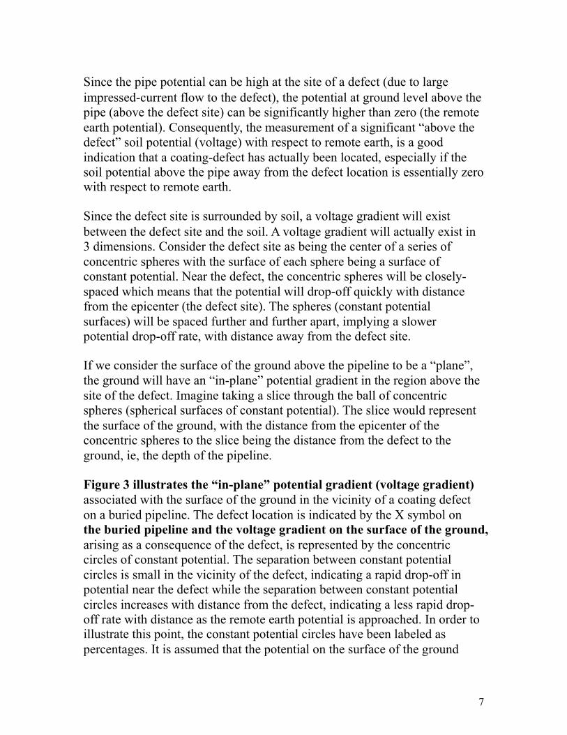
Since the pipe potential can be high at the site of a defect (due to large impressed-current flow to the defect), the potential at ground level above the pipe (above the defect site) can be significantly higher than zero (the remote earth potential). Consequently, the measurement of a significant “above the defect” soil potential (voltage) with respect to remote earth, is a good indication that a coating-defect has actually been located, especially if the soil potential above the pipe away from the defect location is essentially zero with respect to remote earth.

Since the defect site is surrounded by soil, a voltage gradient will exist between the defect site and the soil. A voltage gradient will actually exist in 3 dimensions. Consider the defect site as being the center of a series of concentric spheres with the surface of each sphere being a surface of constant potential. Near the defect, the concentric spheres will be closely- spaced which means that the potential will drop-off quickly with distance from the epicenter (the defect site). The spheres (constant potential surfaces) will be spaced further and further apart, implying a slower potential drop-off rate, with distance away from the defect site.

If we consider the surface of the ground above the pipeline to be a “plane”, the ground will have an “in-plane” potential gradient in the region above the site of the defect. Imagine taking a slice through the ball of concentric spheres (spherical surfaces of constant potential). The slice would represent the surface of the ground, with the distance from the epicenter of the concentric spheres to the slice being the distance from the defect to the ground, ie, the depth of the pipeline.

Figure 3 illustrates the “in-plane” potential gradient (voltage gradient) associated with the surface of the ground in the vicinity of a coating defect on a buried pipeline. The defect location is indicated by the X symbol on the buried pipeline and the voltage gradient on the surface of the ground, arising as a consequence of the defect, is represented by the concentric circles of constant potential. The separation between constant potential circles is small in the vicinity of the defect, indicating a rapid drop-off in potential near the defect while the separation between constant potential circles increases with distance from the defect, indicating a less rapid drop- off rate with distance as the remote earth potential is approached. In order to illustrate this point, the constant potential circles have been labeled as percentages. It is assumed that the potential on the surface of the ground

7

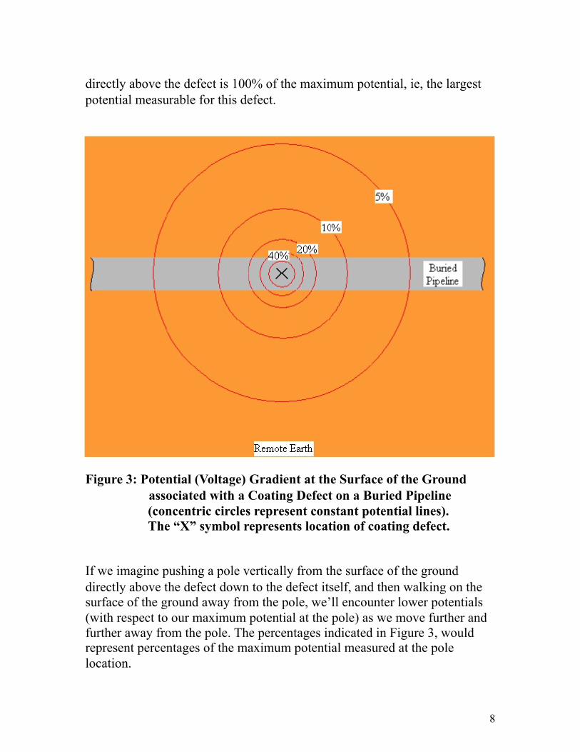
directly above the defect is 100% of the maximum potential, ie, the largest potential measurable for this defect.

Figure 3: Potential (Voltage) Gradient at the Surface of the Ground

associated with a Coating Defect on a Buried Pipeline (concentric circles represent constant potential lines). The “X” symbol represents location of coating defect.

If we imagine pushing a pole vertically from the surface of the ground directly above the defect down to the defect itself, and then walking on the surface of the ground away from the pole, we’ll encounter lower potentials (with respect to our maximum potential at the pole) as we move further and further away from the pole. The percentages indicated in Figure 3, would represent percentages of the maximum potential measured at the pole location.

8

Since such surface potential (voltage) gradients exist above pipeline defects, we can perform soil-to-soil potential difference surveys to detect the defects. Such surveys are know as DCVG surveys (Direct-Current Voltage Gradient surveys).

DCVG surveys can be performed in two different ways: Perpendicular Mode and In-Line (or Parallel) Mode. In the case of Perpendicular DCVG

surveys, an imaginary line drawn between the reference electrodes on the surface of the ground would be perpendicular to the direction of the pipeline and, in the case of In-Line DCVG surveys, an imaginary line drawn between the reference electrodes on the surface of the ground would (ideally) be in-line with the center of the pipeline (directly above the pipeline).

II. 2 Perpendicular DCVG Survey Technique:

As illustrated in Figure 4 below, this technique involves placing a matched- pair of reference electrodes (canes) on the surface of the ground perpendicular to the pipeline direction, with the left-hand cane (red cane) positioned (ideally) over the centerline of the pipe and the right-hand cane (green cane) spaced typically 4 or 5 feet from the left-hand cane. With this cane spacing maintained, the operator walks down the length of the pipeline section triggering voltage recordings every 2.5 feet (or some other length interval, typically 5 to 10 feet). Since the left-hand cane connects to the negative side of the voltmeter (data logger’s voltmeter) and the right-hand cane connects to the positive side of the voltmeter, the voltage recorded at each triggering location is the difference between the soil potentials at the two reference electrode positions in each case. For a detailed discussion on the design and operation of MCM’s reference electrodes used for surveys on buried pipelines, please refer to our CIS Training Manual.

9

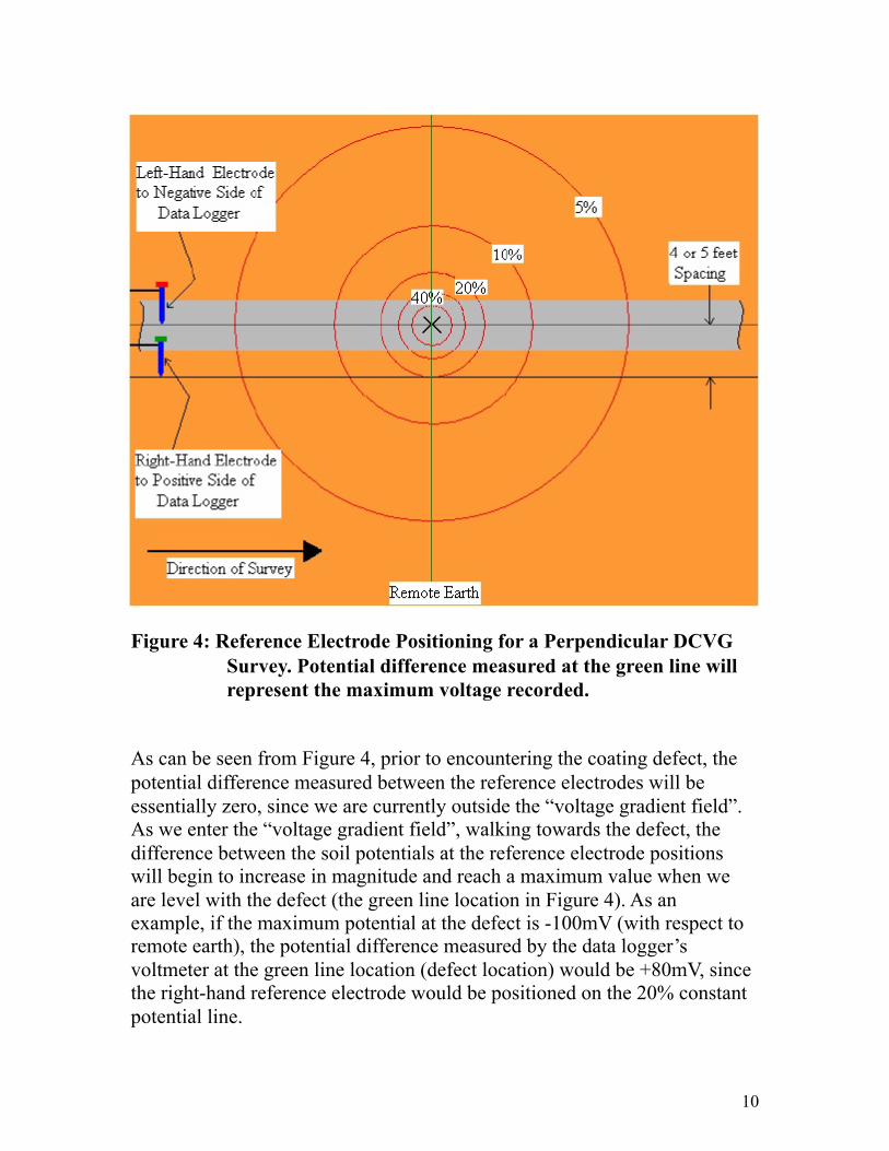
Figure 4: Reference Electrode Positioning for a Perpendicular DCVG

Survey. Potential difference measured at the green line will represent the maximum voltage recorded.

As can be seen from Figure 4, prior to encountering the coating defect, the potential difference measured between the reference electrodes will be essentially zero, since we are currently outside the “voltage gradient field”. As we enter the “voltage gradient field”, walking towards the defect, the difference between the soil potentials at the reference electrode positions will begin to increase in magnitude and reach a maximum value when we are level with the defect (the green line location in Figure 4). As an example, if the maximum potential at the defect is -100mV (with respect to remote earth), the potential difference measured by the data logger’s voltmeter at the green line location (defect location) would be +80mV, since the right-hand reference electrode would be positioned on the 20% constant potential line.

10

The +80mV reading would occur since the voltmeter would subtract -100mV from -20mV to give +80mV [-20mV - (-100mV) = +80mV]. Remember that the right-hand electrode is connected to the positive side of the voltmeter and the left-hand electrode is connected to the negative side of the voltmeter.

If we continue walking past the location of the defect, the difference between the soil potentials at the reference electrode positions will begin to decrease in magnitude and eventually will be zero again as we exit the “voltage gradient field”. Consequently, a profile such as that shown below

in Figure 5 will be observed in the case of Perpendicular DCVG surveys as a coating defect is encountered.

Figure 5: DCVG Voltage as a Function of Electrode Position along Pipeline in the vicinity of a Coating Defect as measured with

electrodes in perpendicular configuration (see Figure 4)

11

II. 3 Definition of DCVG Voltage:

DCVG surveys are performed in the rectifier-current ON/OFF mode, ie, the rectifier current is switched ON and OFF in a cyclic fashion. This allows soil-to-soil potential differences to be recorded during the ON portion of the current cycle and also during the OFF portion of the current cycle.

For DCVG surveys, the MCM data logger’s software calculates the difference between the soil-to-soil potential difference recorded during the ON part of the cycle [delta V(ON)] and the soil-to-soil potential difference recorded during the OFF part of the cycle [delta V(OFF)]. The polarities of both delta V(ON) and delta V(OFF) are also recorded at defect sites (more on these polarities later).

Since delta V(ON) represents the soil-to-soil potential difference with current contributions from the pipeline’s CP system as well as from all other sources (stray interference, foreign pipelines etc.), and, since delta V(OFF) represents the soil-to-soil potential difference with only the “other” current sources contributing, a DCVG recording will represent the soil-to-soil potential difference with only the pipeline’s CP system contributing to the current flow to the defect.

For the remainder of this manual, the term “DCVG voltage” will be taken to mean the difference between the “CP current ON” soil-to-soil voltage reading and the “CP current OFF” soil-to-soil voltage reading.

II. 4 Definition of Total mV:

The, so-called, “Total mV” is the difference between the maximum potential at a defect location and the potential at remote earth, arising due to the CP

system’s contribution to the current flow to the defect. Since, as shown in Figure 4, a typical electrode spacing is 4 to 5 feet and the “voltage gradient field” associated with a defect typically extends a significant distance beyond the right-hand reference electrode location, several measurements are actually required in order to determine the total voltage gradient (Total mV) associated with a defect.

12

II. 5 Procedure to determine Total mV:

When the defect location has been identified as described above (ie, the location where a maximum DCVG voltage reading has been observed), a set of DCVG voltage recordings is made by moving in a straight line perpendicular to the pipeline direction.

Figure 6: Reference Electrode Positions (black dot locations along green line) for “Total mV” Determination

With reference to Figure 6 above, a recording is first made with the left-hand reference electrode positioned over the defect and the right-hand reference electrode positioned at the first black dot location along the green line. The DCVG voltage recorded here is known as the Max mV recording, as this is

13

the maximum DCVG voltage that will be recorded for this defect. This Max mV value becomes the first component of the Total mV determination.

Once the Max mV has been recorded, a DCVG voltage recording is made by placing the left-hand reference electrode in the previous position of the right- hand electrode and moving the right-hand electrode to the location of the second black dot along the green line (all black dots shown in Figure 6 are spaced at 4 to 5 feet intervals). Once a DCVG voltage recording has been made with the electrodes in this position, the electrodes are moved in the same fashion to the next measurement positions and a third DCVG voltage recording is made. This process is continued (typically 3 or 4 measurements are required for a significant defect) until the soil-to-soil potential difference is basically zero, ie, you have reached remote earth.

The MCM data logger’s software will calculate the sum of these DCVG

voltage recordings to generate the “Total mV”. This will represent the voltage gradient on the surface of the ground associated with this defect.

II. 6 Defect “Size” Considerations:

Since “Total mV” represents the voltage gradient on the surface of the ground associated with CP current flowing to a defect, if we can relate the Total mV to a measure of the magnitude of the CP current, we can obtain a measure of the “size” of the defect.

Since the CP current is being switched ON and OFF, we can measure the IR

drop associated with the CP current flowing in the soil (primarily to the defect), which is just the difference in the pipe-to-soil voltage measured during the ON portion of the cycle and the pipe-to-soil voltage measured during the OFF portion of the cycle. Consequently, we can have a measure of the current flowing to the defect (through the IR drop determination), which we can relate to the voltage gradient (Total mV).

II. 7 Definition of % IR:

The magnitude of the voltage gradient on the surface of the ground (Total mV), arising as a consequence of ionic current flowing to the pipe in the vicinity of the defect (CP current magnitude = I), expressed in relationship

14

to the IR voltage drop in the soil (due to the CP current flowing), is a quantity known as the % IR.

% IR = [Total mV/IR drop] x 100

In order to determine the IR drop value to use in the above equation, pipe-to- soil voltages are recorded at the test stations “bracketing” a defect location. The data logger’s software then calculates the difference between the ON

and the OFF pipe-to-soil voltages (IR drop values) at each of the test stations. If the IR values recorded at both test stations are essentially the same, the data logger uses this IR drop value to calculate the % IR value for the defect using the above equation. If, on the other hand, the IR drop values recorded at the two test stations bracketing the defect are significantly different, the data logger’s software will generate an average IR drop value to use in the equation, based on the defect’s location relative to the locations of the two test stations.

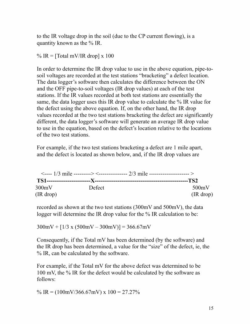
For example, if the two test stations bracketing a defect are 1 mile apart, and the defect is located as shown below, and, if the IR drop values are

<---- 1/3 mile ---------> <--------------- 2/3 mile --------------------- >

TS1-----------------------X-------------------------------------------------TS2 300mV

(IR drop) Defect 500mV

(IR drop)

recorded as shown at the two test stations (300mV and 500mV), the data logger will determine the IR drop value for the % IR calculation to be:

300mV + [1/3 x (500mV – 300mV)] = 366.67mV

Consequently, if the Total mV has been determined (by the software) and the IR drop has been determined, a value for the “size” of the defect, ie, the % IR, can be calculated by the software.

For example, if the Total mV for the above defect was determined to be 100 mV, the % IR for the defect would be calculated by the software as follows:

% IR = (100mV/366.67mV) x 100 = 27.27%

15

II. 8 Summary of DCVG Parameters at Defect Locations

Assuming that IR drop recordings were properly made at “bracketing” test stations and that the appropriate DCVG voltages were recorded at a defect location (with reference to Figure 6 above), the software calculates and stores the following important quantities (in addition to storing all regular DCVG survey data).

For each “marked” defect site: > Maximum delta V(ON) or Max mV(ON): Magnitude and Polarity > Maximum delta V(OFF) or Max mV(OFF): Magnitude and Polarity > Max mV (Max mV(ON) – Max mV(OFF)): Magnitude (always positive) > Total mV: Magnitude > % IR: Magnitude

II. 9 Polarity Considerations

By noting the polarities of the maximum soil-to-soil potential difference recorded with rectifier-current ON and rectifier-current OFF at a defect site, we can determine the corrosion condition of the defect with the CP system

current flowing (ON state) and without the CP system’s impressed current flowing (OFF state).

If net current is flowing to the defect, the potential at the defect will be negative, relative to remote earth; however, the maximum delta V recording will have a positive value, due to the positioning of the “positive” and “negative” reference electrodes. This is a cathodic condition.

If net current is flowing away from the defect into the soil, the potential at the defect will be positive with respect to remote earth; however, the maximum delta V recording will have a negative value. This is an anodic condition.

Since we are able to record the polarity of Max mV(ON) and Max mV(OFF), we can determine the corrosion condition of the defect both when the CP current is impressed and when the CP current is not flowing to the defect. The best case scenario is cathodic/cathodic, however, cathodic/anodic is also acceptable, since in this case, the CP system’s impressed current is doing its job, ie, it is preventing corrosion taking place

16

at the defect site. The worst case scenario would be anodic/anodic, since in this case the defect is not protected even with CP current flowing.

II. 10 In-Line (Parallel) DCVG Survey Technique:

There is a second method of performing DCVG pipeline surveys, known as In-Line (or Parallel) mode DCVG surveys.

In this case, DCVG voltages are recorded in a close-interval fashion by placing the reference electrodes in-line with the pipeline (directly over the pipeline), as opposed to placing the reference electrodes perpendicular to the pipeline direction.

This technique is illustrated in Figure 7 below.

As can be seen from Figure 7, as the operator enters the “voltage gradient field” associated with the defect and places the reference electrodes as indicated with the right-hand electrode connected to the positive side of the data logger’s voltmeter and the left-hand electrode connected to the negative side of the voltmeter, the DCVG voltage measured will begin to increase and have a positive polarity.

As the defect location is approached, the DCVG voltage will increase more sharply, since the circles of constant potential are spaced closer together. A

maximum DCVG voltage will be measured when the left-hand reference electrode is directly over the defect.

As indicated in Figure 7, however, the DCVG voltage will drop to zero when the operator is straddling the defect, since in this position, the reference electrodes will be measuring the same potential and, hence, the potential difference between them will be zero.

Continuing down the line, with the right-hand electrode directly over the defect, the DCVG voltage will again have a maximum value, however, this time the polarity will be negative.

Finally, as the operator continues down the line, the magnitude of the DCVG

voltage measured will decrease quickly near the defect and then decrease more gradually moving further away from the defect.

17

Figure 7: In-Line DCVG Survey Technique

Consequently, the DCVG voltage profile recorded in the vicinity of a defect will be considerable different in appearance from that observed in the case of a Perpendicular DCVG survey (see Figure 5).

18

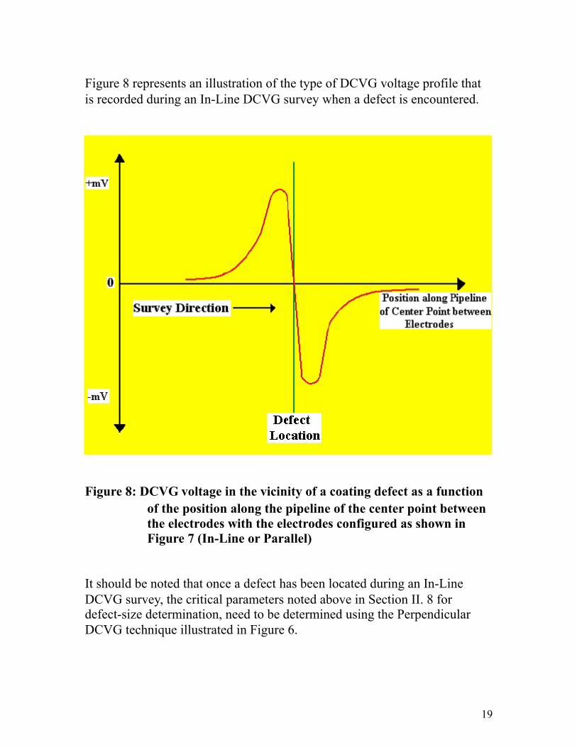
Figure 8 represents an illustration of the type of DCVG voltage profile that is recorded during an In-Line DCVG survey when a defect is encountered.

Figure 8: DCVG voltage in the vicinity of a coating defect as a function

of the position along the pipeline of the center point between

the electrodes with the electrodes configured as shown in

Figure 7 (In-Line or Parallel)

It should be noted that once a defect has been located during an In-Line DCVG survey, the critical parameters noted above in Section II. 8 for defect-size determination, need to be determined using the Perpendicular DCVG technique illustrated in Figure 6.

19

SECTION III: HOW TO SETUP THE G1 DATA-LOGGER

FOR DCVG SURVEYS

The following section outlines the steps required to setup the G1 data-logger to participate in DCVG pipeline survey applications. The setup process establishes the conditions of the particular survey about to be performed and identifies the section of pipeline that is about to be examined by the DCVG

application. The setup process (and this is very important) also establishes a file in which the voltage recordings (survey data) will be stored. At the completion of the survey, DCVG survey data can then be retrieved by a PC

that is in communication with the data-logger by accessing the file in which the survey data are stored.

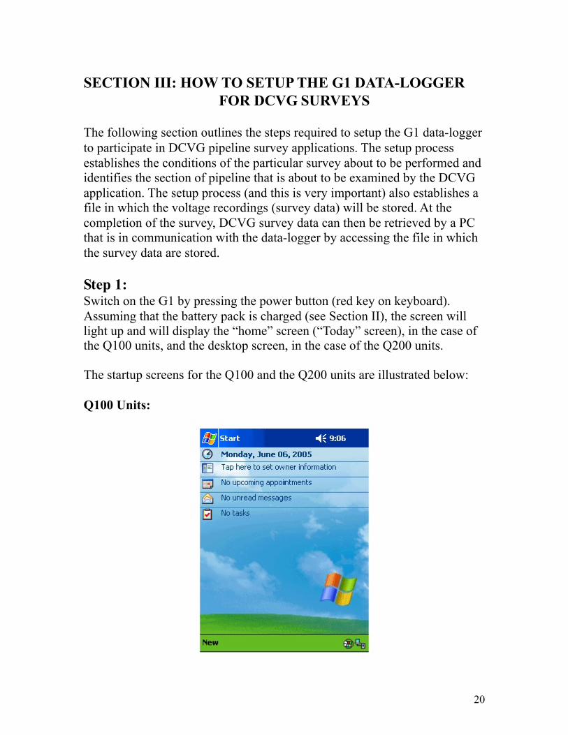
Step 1: Switch on the G1 by pressing the power button (red key on keyboard). Assuming that the battery pack is charged (see Section II), the screen will light up and will display the “home” screen (“Today” screen), in the case of the Q100 units, and the desktop screen, in the case of the Q200 units.

The startup screens for the Q100 and the Q200 units are illustrated below:

Q100 Units:

20

Q200 Units:

Step 2: In the case of the Q100 units, tap on the “Start” button on the “Home” screen. This will pull up the main menu.

Step 3: In the case of the Q100 units, tap on the G1 PLS button on the main menu. In the case of the Q200 units, double-tap on the G1PLS icon on the desktop or tap on the start icon (bottom left-hand corner of desktop), tap on the “Programs” button and tap on the G1PLS button.

In either case, (Q100 or Q200 units), the survey screen shown below will be displayed.

Note: In the case of the Q200 units, the menu items are arrayed along the top of the screen.

21

Step 4: Tap on “Survey” in the menu bar along the bottom of the above screen. The screen shown below will appear.

Under “Survey” there are several options. If this is a new survey (not a continuation of a previous survey) tap on “New Survey”. The screen shown below will appear.

22

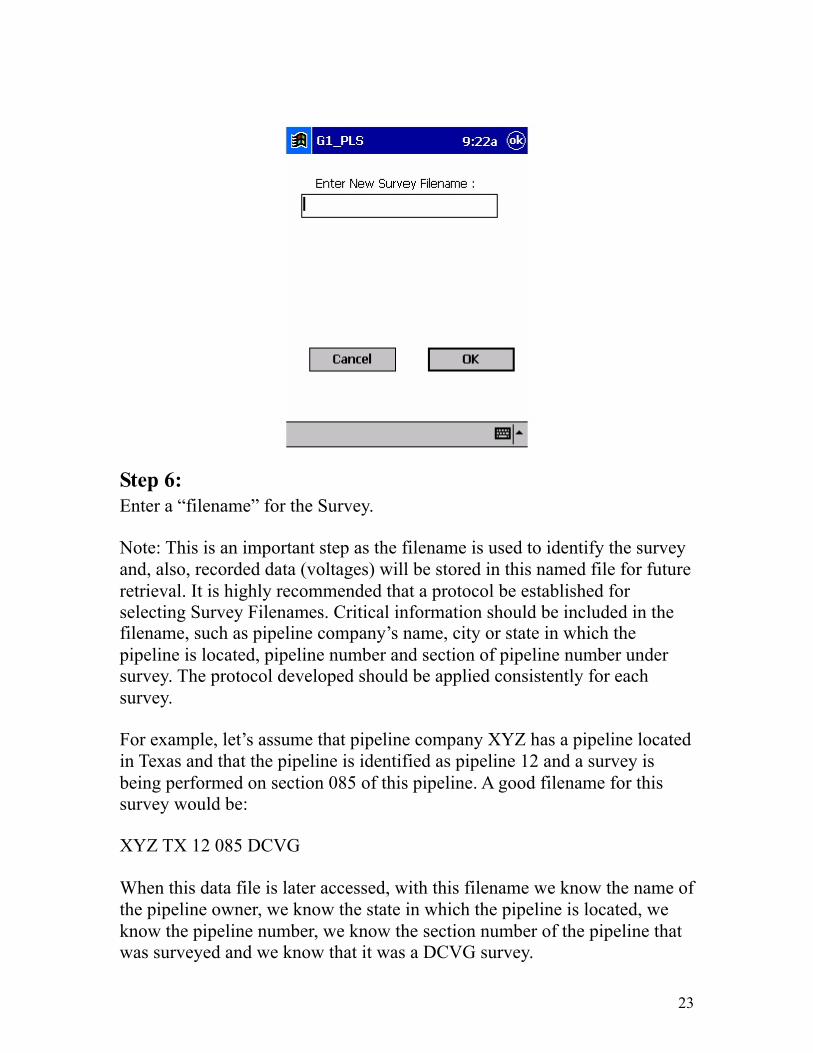
Step 6: Enter a “filename” for the Survey.

Note: This is an important step as the filename is used to identify the survey and, also, recorded data (voltages) will be stored in this named file for future retrieval. It is highly recommended that a protocol be established for selecting Survey Filenames. Critical information should be included in the filename, such as pipeline company’s name, city or state in which the pipeline is located, pipeline number and section of pipeline number under survey. The protocol developed should be applied consistently for each survey.

For example, let’s assume that pipeline company XYZ has a pipeline located in Texas and that the pipeline is identified as pipeline 12 and a survey is being performed on section 085 of this pipeline. A good filename for this survey would be:

XYZ TX 12 085 DCVG

When this data file is later accessed, with this filename we know the name of the pipeline owner, we know the state in which the pipeline is located, we know the pipeline number, we know the section number of the pipeline that was surveyed and we know that it was a DCVG survey.

23

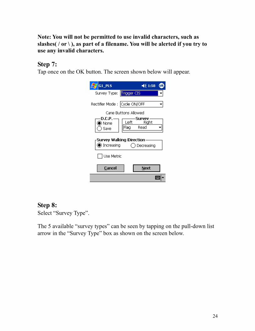
Note: You will not be permitted to use invalid characters, such as slashes( / or \ ), as part of a filename. You will be alerted if you try to use any invalid characters.

Step 7: Tap once on the OK button. The screen shown below will appear.

Step 8: Select “Survey Type”.

The 5 available “survey types” can be seen by tapping on the pull-down list arrow in the “Survey Type” box as shown on the screen below.

24

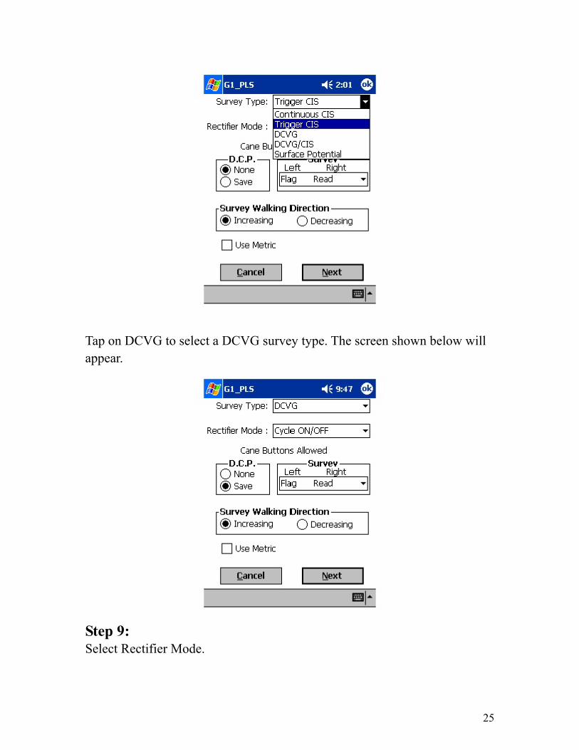
Tap on DCVG to select a DCVG survey type. The screen shown below will appear.

Step 9: Select Rectifier Mode.

25

Select “Cycle ON/OFF” in the “Rectifier Mode” field by tapping on the pull-down list arrow button and highlighting “Cycle ON/OFF”. This is the only appropriate rectifier mode for DCVG surveys.

Step 10: Make “Cane Button” Functionality Choices

Typically, for DCVG surveys, you would “trigger” DCVG voltage recordings using the right-hand (positive) reference electrode and the left- hand reference electrode’s push button switch would be used to designate the location of survey flags. For this case, your “Survey” selection for canes would be “Flag Read” as shown in the above screen. The other options can be viewed by tapping on the pull-down list arrow button in the Survey field.

You can also use either cane button when recording voltages at D.C.P.’s (data collection points (devices)) to “save” a device reading, as opposed to tapping on the “save” button on the device screen. For example, with the selection as indicated on the above screen, device readings would be recorded automatically by triggering either cane button, which is the “save” option. If you prefer to tap buttons on the screen at Devices, select the “none” option in the D.C.P. box.

Note: When “Marking” DCVG anomalies, the cane push-button functionality becomes “accept”, regardless of whether “save” or “none” is selected here.

Step11a: Select Walking Direction

Finally on the above screen, you should indicate whether station numbers will be increasing or decreasing as you proceed in the survey direction by tapping on either “Increasing” or “Decreasing” in the “Survey Walking Direction” box.

Step 11b: Make selection of “Metric” units if required.

26

By checking off the box labeled “Metric”, the reading interval (distance between voltage recordings) and the flag internal (flag spacing) will be displayed in meters, as opposed to feet.

Tap on the “Next” button on the above screen.

Step 12: Select GPS Type

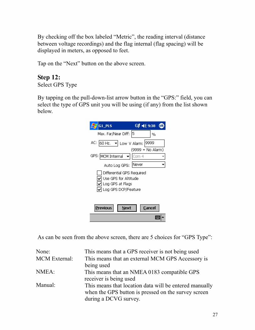
By tapping on the pull-down-list arrow button in the “GPS:” field, you can select the type of GPS unit you will be using (if any) from the list shown below.

As can be seen from the above screen, there are 5 choices for “GPS Type”:

None: MCM External:

NMEA:

Manual:

This means that a GPS receiver is not being used This means that an external MCM GPS Accessory is being used This means that an NMEA 0183 compatible GPS

receiver is being used This means that location data will be entered manually when the GPS button is pressed on the survey screen during a DCVG survey.

27

MCM Internal: This means that the G1’s internal GPS unit will be used (a Garmin (Model 15L) WAAS-enabled receiver)

Select the appropriate choice by tapping on your selection.

When using an external GPS unit, you need to select the Com Port that you’ll be using on the G1 (see above screen). The connector terminal on the left-hand side of the data-logger (facing the bottom side) is the COM 1 Port and the terminal on the right-hand side is the COM 4 Port. It is recommended that you select the COM 4 Port for your external GPS unit in order to avoid potential conflicts with ActiveSync which uses COM 1.

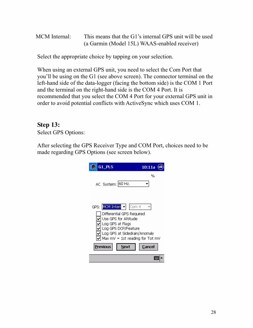
Step 13: Select GPS Options:

After selecting the GPS Receiver Type and COM Port, choices need to be made regarding GPS Options (see screen below).

28

If a GPS accessory has been selected for use with the data-logger for a particular DCVG survey, all, or some of the functions available can be enabled (box ticked). A box can be “ticked” or “unticked” by tapping inside the box. The GPS options available are as follows:

Differential GPS Required: This box should be ticked if you only want differentially-corrected GPS

position data to be logged by the data-logger. If this box is left unticked, it means that you will allow the G1 data-logger to log either standard GPS

position data or differentially-corrected GPS position data.

Note: Logging “Standard” GPS position data is usually better than having no data logged at all, which would be the case if you checked this box and for some reason your GPS receiver was not outputting differentially- corrected position data. Consequently, it may be preferable to leave this box unchecked, unless it is imperative that you exclusively log differentially- corrected GPS position data.

Use GPS Altitude: If this box is ticked, altitude data will be included with the position data whenever GPS data is logged. (Note: Altitude data on some GPS units is not particularly accurate in survey applications).

Log GPS at Flags: If this box is ticked, GPS position data will be logged automatically at flags when either the flag button is tapped (directly on the Survey screen) or when the push-button on the designated “flag cane” is pressed.

Log GPS at DCP/Feature: If this box is ticked, GPS position data will be logged automatically at “Devices” or “Geo-Features” when either the “Device” button is tapped on the Survey screen and a “Device” reading is logged or when the “Geo-Feat.” button is tapped on the Survey screen and a geo-feature is registered.

Log GPS at Sidedrain/Anomaly: If this box is ticked, GPS location data will be logged automatically when DCVG defects (anomalies) are “marked”.

29

Auto Log GPS: By tapping on the drop down menu button in the “Auto Log GPS” field, the selections available will be displayed as indicated below.

By selecting one of these options, you can elect to have the GPS position data logged automatically at every survey reading, at every second reading, at every fifth reading, at every tenth reading, or not at all (never) at survey readings.

Step 14: Select Max mV Reading to be First Reading in Total mV Determination.

The last box in the above screen is actually not related to GPS Options. If this box is ticked, the Max mV voltage value recorded at an anomaly location will automatically become the first voltage value used by the data- logger’s software to calculate the Total mV (total voltage gradient). Otherwise, if this box is not ticked, you will have to repeat the Max mV

recording a second time as part of the Total mV determination process.

Step 15: Finally on the above screen, select the electricity supply operating frequency of the country in which you are performing the surveys (60Hz or 50Hz). For the U.S., select 60Hz.

30

Tap on the “Next” button on the above screen. The screen shown below will appear.

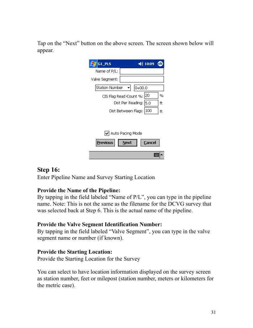
Step 16: Enter Pipeline Name and Survey Starting Location

Provide the Name of the Pipeline: By tapping in the field labeled “Name of P/L”, you can type in the pipeline name. Note: This is not the same as the filename for the DCVG survey that was selected back at Step 6. This is the actual name of the pipeline.

Provide the Valve Segment Identification Number: By tapping in the field labeled “Valve Segment”, you can type in the valve segment name or number (if known).

Provide the Starting Location: Provide the Starting Location for the Survey

You can select to have location information displayed on the survey screen as station number, feet or milepost (station number, meters or kilometers for the metric case).

31

Whichever selection you make here will determine how you enter your starting location information.

For example, if your pipeline locations are represented by station numbers, you would select “Station Number” from the drop down list and you would enter a starting location for the survey in the form of a station number. [If you do not know the station number where you’re beginning your survey, enter 0+0.0].

As an example, if you are working on pipeline ABC within valve segment 45 and you are about to begin a DCVG survey at station number 12+00.0, your screen would be as shown below.

Step 17: Select Voltage Recording Interval (Distance Between Recordings)

By tapping in the field on the above screen labeled “Distance Per Reading”, you can type in the voltage reading interval (distance in feet (or in meters for the metric case) expected between recordings) for the DCVG survey. In DCVG work this expected interval distance is typically 5.0 feet.

32

Step 18: Select Survey Flag Interval (Distance Between Survey Flags)

By tapping in the box on the above screen labeled “Distance Between Flags”, you can type in the survey flag interval (distance between survey flags in feet, or in meters for the metric case) for the section of pipeline being measured. Typically, survey flags are located at 100 feet intervals.

Step 19: Select the maximum permissible error between the actual number of recordings made between 2 survey flags and the expected number of recordings.

By tapping in the field labeled, “CIS Flag Read Count %”, you can type in the maximum permissible error. For example, the maximum permissible error is indicated as 20% on the above screen. If the recording interval is expected to be 5.0 feet and the survey flag separation is 100 feet, that means that 20 recordings are expected. If, however, only 15 recordings are actually made between survey flags, an error window will appear on the screen, since there is a 25% difference between the expected and actual number of recordings made. No error window will appear if the difference is less than 20% for this example, ie, you could have a minimum of 16 recordings and a maximum of 24 recordings between survey flags to stay within the 20% (max.) error allowance.

Step 20: Select whether or not you would like the recordings to be uniformly spaced between survey flags, in cases where less than or greater than 20 recordings are made.

By tapping in the box labeled, “Auto Pacing Mode”, and inserting a tick in the box, you will enable the data-logger to automatically adjust the actual recordings and space them evenly over the flag spacing distance, regardless of the actual number of recordings made. Again, enabling this selection is recommended.

Tap on the Next button on the above screen. The screen shown below will appear.

33

Step 21: Provide the Work Order Number for the DCVG survey.

By tapping in the field on the above screen labeled, “Work Order #”, you can type in the work order number for the DCVG survey.

Step 22: Provide Your Name.

By tapping in the field labeled, “Technician Name”, you can type in your name or the name of your supervisor. If you use your supervisor’s name here, you might add your own name in the Comments Section.

Step 23: Provide Comments.

By tapping in the field labeled, “Comments/Description”, you can enter any comments you might have regarding the survey (perhaps weather conditions, soil conditions etc.). Also shown on the above screen are the Survey (File) Name and the Survey Start Date and Time.

34

Note: Do not attempt to change the File Name indicated here as this identification will be required by the ProActive software to transfer your DCVG survey data to your PC.

Tap in the Next button on the above screen. The screen shown below will appear.

Step 24: Select Voltmeter Settings and Current Interruption Cycle.

Voltmeter Reading Mode DCVG surveys are performed with the CP system’s rectifier-current switched ON and OFF in a cyclic fashion and, as can be seen from the above screen, there are two choices available for the data-logger’s voltmeter “Read Mode”. The choices are “On/Off Pairs (DSP mode)” and “On/Off Pairs (GPS Sync)”.

Note: On/Off Pairs (Min/Max) is not a option here since DCVG surveys require a measurable difference between On and Off voltages, ie, they require a significant IR drop.

35

On/Off Pairs (DSP mode): In this mode, the voltmeter uses digital signal processing techniques to determine the “flat” portions (for both the On and Off parts of the cycle) of the rectifier-current cycle. ∆V values are then determined for the On and the Off portions of the cycle from which the DCVG voltage is calculated [∆V(On) minus ∆V(Off)].

For these measurements to be successful, the data probes (reference electrode canes) must remain in good electrical contact with the soil for at least one rectifier-current waveform period following the initial contact of the probes with the soil, for a stable DCVG voltage value to be displayed.

On/Off Pairs (GPS Sync): This voltmeter mode could be selected if you were using an MCM GPS

receiver on your DA Meter and current-interrupter switches equipped with GPS units were being employed on the rectifiers. In this case, ∆V(On) and ∆V(Off) values are based on potentials measured at pre-determined sampling times on each waveform cycle, which are synchronized with the current-interruption switching timing.

Also, in this case, you would tap on the “GPS Settings” button, which would bring up the screen shown below.

You are being asked here to make several selections.

36

First, select the type of GPS unit you will be using (the data-logger’s Internal unit or the MCM External unit ONLY).

Next, enter your “On Delay” and your “Off Delay” selections by tapping in the appropriate box and typing in the requested delay time in milliseconds. These delay times are employed so that any spiking in the voltage waveform

that might occur as the rectifier-current is switched from ON to OFF and from OFF to ON does not become a factor in the voltmeter’s determination of the “true” ON and OFF voltage values for each DCVG measurement. For example, if 150 ms was selected for the “Off Delay”, the data logger would record the voltage value sampled 150 ms after the rectifier-current was switched from the ON to the OFF state. Also, if 150 ms was selected for the “On Delay” the data logger would record the voltage value sampled 150 ms after the rectifier-current was switched from the OFF to the ON state.

Next, select your current interrupter’s “Downbeat” timing. As indicated by tapping on the pull-down-list arrow button in the “Downbeat” box, there are 3 industry-standard selection choices; Each Minute, Each Hour and Midnight. If “Each Minute” is an option for your current interrupter, we suggest making this selection. The “Each Minute” designation indicates to the data-logger that a new interruption cycle will begin at the top of each minute. Consequently, the data-logger can reference its timing to the top of each minute. In this instance, your On plus Off times (your waveform

period) should be an even multiple of 60.

Again, for these measurements to be successful, the data probes (reference electrode canes) must remain in good electrical contact with the soil for at least one rectifier-current waveform period following the initial contact of the probes with the soil, for a stable DCVG voltage value to be displayed.

Finally, if your interruption cycle starts with the current in the ON state (the first transition is from ON to OFF), place a tick in the “Start Cycle” box (remove the tick if the opposite is true).

After making your “GPS Settings” selections, tap on the “OK” button which will return you to the Voltmeter Settings screen.

37

Select the Cycle On/Off Times: The specific On and Off times for the particular current-interruption waveform cycle that will be employed during your DCVG survey should be entered in the “Cycle (ms)” fields. The On and the Off times should be entered in milli-seconds.

Note: After a time period corresponding to at least one waveform period (On time plus Off time), the DCVG voltage value displayed on the DA

Meter survey screen should stabilize (assuming that the data probes are making good electrical contact with the soil) and a DCVG voltage recording can be triggered.

Consequently, the rate at which DCVG voltages can be captured and saved depends critically on the interruption waveform period. This is a particularly important issue in the case of large period waveforms. For example, if a 10 second On and a 2 second Off waveform is employed (12 second waveform

period), stabilization times up to 12 seconds could be possible before each DCVG voltage recording can be made. In contrast, the stabilization period would be only on the order of one second for a 700ms On, 300ms Off interruption cycle.

Select Voltmeter Range and Input Impedance Settings: By tapping on the pull-down list arrow button in the “Range” field, you can select the voltmeter range and input impedance settings for your application.

The recommended settings for the voltmeter for DCVG surveys are 5.7 Volts (full-scale) and an input impedance value of 400MOhm, These settings provide a relatively-fast response time (~80 ms), which is important in rectifier-current-interrupted applications and also a relatively-sensitive scale with regard to the magnitude of the DCVG voltages that you’ll be measuring. Note: Caution has to be exercised if any of the ranges beginning with the number 4 (for example, 4V, 400mV or 40mV) are selected for DCVG

applications, since these represent relatively-slow response settings. Such settings provide a higher level of AC filtering (less noise), but at the expense of speed of response. Rather than the response time of 80ms for the 5.7V

range, these settings have a response time greater than 1 second. Consequently, such settings are not appropriate for fast current-interruption cycles, ie, interruption On and Off times shorter than 1 second, as true On and Off potentials would not be recorded.

38

Step 25: Pull-up “Active” Survey Screen

By tapping on the “OK” button on the Voltmeter Settings screen, the “active” Survey screen would appear and you would be ready to proceed with your DCVG survey.

An example starting “active” Survey screen is shown below.

In the above “active” DCVG survey screen, the direction of the arrow

(pointing to the left or pointing to the right) depends on the polarity of the DCVG voltage being measured. In the above case, the voltage being measured was positive which produced an arrow pointing to the left. The opposite would be true if the DCVG voltage reading had been negative (ie, the arrow would point to the right). With the reference electrodes properly positioned, the polarity of the DCVG

voltage will always be positive in the case of perpendicular DCVG surveys. In this case, the arrow on the survey screen will always point back to the pipe.

39

However, a change in arrow direction will be evident when performing parallel, or in-line, measurements in the vicinity of a DCVG anomaly (coating defect). In this case, the arrow will always point in the direction of the defect location on the pipe with respect to where you are currently standing. As you approach the defect, the arrow will point towards the upcoming defect location and when you are past the defect, the arrow will point back to the defect location. Consequently, performing in-line measurements in the vicinity of a defect can be a good way to pin-point its precise location, by monitoring the arrow’s polarity switches. When you are actually straddling a defect location (with the reference electrodes in-line with the pipe), the DCVG voltage will be zero (ie, neither positive nor negative).

Also, with respect to the above “active” survey screen, as DCVG voltages are recorded by the data-logger, the “Total Distance” (total distance from the start of the survey) parameter will increase in increments of 5.0 feet , or whatever the “Distance Per Reading” value was that was entered back at Step 17. (Distances would be in meters for the metric case).

Also, the “Distance From Flag” parameter will increase in the same increments as voltages are recorded. The difference in this case, however, will be that when each survey flag is registered, this distance parameter will begin again at zero. In other words, this will show the distance you are assumed by the data-logger to have traveled from the last flag that you encountered (and registered).

You are now ready to perform a DCVG Survey.

40

SECTION IV: TEST EQUIPMENT HOOK-UPS FOR

DCVG SURVEYS

IV. 1 How to make Cable Hook-Ups for DCVG Surveys

The cable connections for DCVG surveys employing MCM test equipment are illustrated in Figure 9.

Figure 9: Cable Connections for Hook-Up of MCM’s DCVG Survey Test Equipment

41

As can be seen from Figure 9, a pair of canes (reference electrodes – see our CIS Training Manual) is illustrated, the left-hand cane (RED-handled cane) and the right-hand cane (GREEN-handled cane). These canes, which will be placed on the soil above the pipeline in either the “Perpendicular” or the “In-Line” configuration (see Section II), have push buttons on top of the handles so that the operator can “trigger” voltage recordings on his command at each of the pipeline survey measurement locations as well as at “Devices” and “Geo-Features”. See Section III, Step 10 for a discussion on cane button functionality (Step 10 of the G1’s Set Up Process).

The canes (data probes) are connected as shown to the “input” terminals of the dual-probe adapter and the “output” terminal of the adapter is connected to a 5-pin Data Probe Connector socket on the top side of the G1.

NOTE: The left-hand reference electrode (red-handled cane) is connected to the dual probe adapter via a “black-band” cable while the right-hand reference electrode (green-handled cane) is connected to the dual-probe adapter via a “red-band” cable. This is important since the right-hand reference electrode connects to the positive side of the data logger’s voltmeter, while the left-hand reference electrode connects to the negative side of the voltmeter. The red-band and the black-band cables can be connected to either one of the dual-probe adapter’s “input” terminals.

The GPS Antenna illustrated on the top side of the G1 in Figure 9 represents the antenna employed by the data-logger’s internal GPS receiver. External GPS receiver units, if employed, would be connected to the data-logger via one of the two USB COM terminals located on the bottom side of the G1. (The right-hand-side COM Port (COM 4) is recommended. With either the internal unit or an external GPS unit, the location of items such as flags, devices, geo-features and anomalies can be recorded during the performance of a DCVG survey, either manually by tapping on the “Log GPS” button on the survey screen at each critical location or automatically, by pre- programming the data-logger as described above in Section III (Step 13).

IV. 2 How to Attach Cables and Accessories to the G1

The terminals on the top side of the G1 data-logger for the various connections described above are illustrated in Figure 10 below.

42

Figure 10: Connection terminals on top side of G1 Data-Logger

The 5-pin Data Probe Connector Socket is shown above as Terminal 1. As discussed above, the reference electrode canes are connected to this terminal via the dual probe adapter. Again, the reference electrodes are effectively connected to the positive (green-handled cane) or negative (red-handled cane) sides of the voltmeter with this connection.

Consequently, the red and black banana plug terminals (Terminals 2 and 3) are not used in this DCVG survey application.

However, the red banana plug terminal (Terminal 3) is used to connect (temporarily) a test cable between the G1 and a test station (TS), in order to record pipe-to-soil voltages and voltage waveforms prior to beginning a DCVG survey (see Sections V. 2 and V. 3).

The GPS Antenna shown above is employed by the data-logger’s internal GPS unit. External GPS units are connected to either the left-hand-side COM Port (COM 1) or the right-hand-side COM Port (COM 4) located on the bottom side of the data-logger. As mentioned above, in Section III, the COM 4 Port is recommended to avoid conflict with ActiveSync.

43

SECTION V: HOW TO PERFORM DCVG SURVEYS

V. 1 How to Carry the Test Equipment During a DCVG Survey

With the MCM test equipment connected as shown in Figure 9 (Section IV), and the G1 data-logger set up as described in Section III, you are ready to perform a DCVG survey.

To make a pipeline survey more manageable, MCM has developed a special harness (belt pack) which allows the G1 to be carried around the waist area in a “hands-free” fashion, allowing the individual to be able to position the reference electrodes (canes) on the ground (every 5.0 feet, or so, down the length of the pipeline) and to be able to “trigger” the push button canes when appropriate to do so.

With the harness assembly, the G1 sits on a tray at waist level allowing the operator to view the screen at all times and to make any selections required by tapping on the screen. Also, the dual-probe adapter shown in Figure 9, is attached to the underside of the tray, allowing convenient (5 pin cable) connection of the adapter’s “output” to the G1. [Again, this will effectively connect the green-handled reference electrode cane to the positive side of the data logger’s voltmeter and the red-handled reference electrode cane to the negative side of the voltmeter].

In addition, an external GPS receiver unit (together with its battery pack and antenna), if the internal GPS unit is not being employed, can also be attached to the waist band of the harness, typically on the operator’s back at waist level, with the antenna rising to above-head height.

V. 2 Readings to Take at Beginning of a DCVG Survey

It is important to begin your DCVG survey at a test station or at some other device that allows you to make electrical connection temporarily to the pipeline. Connection to the pipeline is required so that an IR drop value can be determined for use in the software’s calculation of % IR. (see Section II. 7).

44

Note: A significant IR drop value is necessary in order to be able to detect DCVG anomalies. For example, for the 5.7V, 400MΩ voltmeter setting, a minimum IR drop value of ~200mV is suggested for the following reason:

If it is assumed that you would like to “mark” defects having, as a minimum, a 10% IR “size”, the minimum Total mV value, in the example case of a 200mV IR drop, would be 20mV. This means, in

turn, that the minimum “Max mV” value that you’d be measuring would only be ~10mV or so, since, typically, about 50% of the total voltage gradient is accounted for in the first side drain reading (the Max mV reading). Since the noise level associated with the 5.7V, 400MΩ

voltmeter setting is around ±5mV, you can see why ~200mV would be a suggested minimum IR drop value. An IR drop value around 500mV

would make small size anomaly detection significantly easier.

Alternatively, a lower noise level voltmeter setting could be used, for example, the 400mV, 10MΩ setting, which as a noise level around

±1mV. In such a case, the minimum IR drop value required to reasonably detect a 10% anomaly would be around 40mV, by the above reasoning. However, as indicated in Step 24 of Section III (Select Voltmeter Range and Input Impedance Settings), caution has to be exercised when selecting a range beginning with the number 4, such as 400mV or 40mV, as these settings have slower response times than the 5.7V range, for example. Since, the response time on the 400mV setting is around 1 second (as opposed to 80ms for the 5.7V setting), the current interruption On and Off times need to both be greater than 1 second, so that the voltmeter will read accurate On/Off potentials for each cycle.

With the CP system’s current being switched ON and OFF in a prescribed cyclic fashion, you can make pipe-to-soil voltage recordings with a slight adjustment to the equipment hook-up arrangement shown in Figure 9.

By temporarily disconnecting the positive (green-handled) cane from the dual-probe adapter and connecting a test cable from the red banana plug terminal on the top side of the G1 to the test station, you can record pipe-to- soil voltages during the ON and the OFF cycles, which will allow the software to determine the IR drop at this test station location.

45

For the pipe-to-soil measurements, the negative cane (red-handled) cane should be positioned over the pipe. As described below (Section V. 4), a device reading can then be taken by tapping on the “Device” button on the Survey screen and proceeding as indicated. It is also recommended that you examine and record the pipe-to-soil Voltage Waveform at this location as described below (Section V. 3)

V. 3 How to Record the Pipe-To-Soil Voltage Waveform

When you are performing a DCVG survey, it is recommended that you examine the pipe-to-soil voltage waveform at your starting location (starting test station) and it is suggested that you make a recording of this voltage waveform using your G1 data-logger. The nature of the voltage waveform

that you are examining will reflect the nature of the rectifier-current waveform that is currently in effect on your pipeline.

With the red-handled reference electrode cane making good electrical contact with the soil above the pipe at the first test station and a test cable connected from the test station to the red banana plug terminal on the G1, you can examine the pipe-to-soil voltage waveform, either by tapping on the WAVE button at the bottom of the Survey screen or by tapping on “Options” followed by “Wave”. The screen shown below will appear.

46

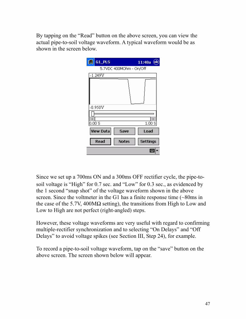
By tapping on the “Read” button on the above screen, you can view the actual pipe-to-soil voltage waveform. A typical waveform would be as shown in the screen below.

Since we set up a 700ms ON and a 300ms OFF rectifier cycle, the pipe-to- soil voltage is “High” for 0.7 sec. and “Low” for 0.3 sec., as evidenced by the 1 second “snap shot” of the voltage waveform shown in the above screen. Since the voltmeter in the G1 has a finite response time (~80ms in the case of the 5.7V, 400MΩ setting), the transitions from High to Low and Low to High are not perfect (right-angled) steps.

However, these voltage waveforms are very useful with regard to confirming multiple-rectifier synchronization and to selecting “On Delays” and “Off Delays” to avoid voltage spikes (see Section III, Step 24), for example.

To record a pipe-to-soil voltage waveform, tap on the “save” button on the above screen. The screen shown below will appear.

47

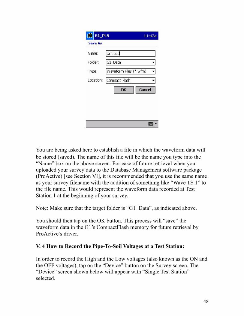
You are being asked here to establish a file in which the waveform data will be stored (saved). The name of this file will be the name you type into the “Name” box on the above screen. For ease of future retrieval when you uploaded your survey data to the Database Management software package (ProActive) [see Section VI], it is recommended that you use the same name as your survey filename with the addition of something like “Wave TS 1” to the file name. This would represent the waveform data recorded at Test Station 1 at the beginning of your survey.

Note: Make sure that the target folder is “G1_Data”, as indicated above.

You should then tap on the OK button. This process will “save” the waveform data in the G1’s CompactFlash memory for future retrieval by ProActive’s driver.

V. 4 How to Record the Pipe-To-Soil Voltages at a Test Station:

In order to record the High and the Low voltages (also known as the ON and the OFF voltages), tap on the “Device” button on the Survey screen. The “Device” screen shown below will appear with “Single Test Station” selected.

48

By tapping the “Next” button on the above screen, the screen shown below

will appear.

As shown above, the High and Low voltage readings (for each cycle) measured at the test station will be displayed on this screen. The voltages shown above represent a “snap-shot” in time.

49

The software will calculate the difference between the High and the Low

voltage recordings (which is the IR drop) and use this quantity in additional calculations (%IR calculations). The "Use reading for DCVG signal strengh" setting defaults to "Yes" (box checked). The IR drop is also referred to as the “signal strength”. You should then tap on the “Save” button to save this data. Note 1: You should perform pipe-to-soil measurements at each test station you encounter in order that the software can perform the linear interpolation calculation described in Section II. 7, when necessary, to determine an “average” signal strength (IR drop) to apply at each defect location between test stations. Note 2: You can "edit" which device readings (pipe-to-soil readings) will be used in signal strength calculations using the following procedure: Tap on the "Options" menu, tap on "Edit Survey Data", tap on "Retrieve", locate and highlight the device in question (via the "Mode" column) and tap on the "View Details" button. Next, scroll across to the "Use for %IR" column and highlight the cell. Next, select Y or N.

V. 5 How to Locate and “Mark” Defects

As mentioned above, when possible, the CP system should be adjusted to provide a signal strength (IR drop) of at least 200mV, in the case of the 5.7V, 400MΩ voltmeter setting. This will make it easier to find the smaller defects as well as the larger ones.

Once you have recorded the pipe-to-soil voltages and observed the magnitude of the signal strength (IR drop), you should disconnect the test cable from the G1’s red banana plug terminal and reconnect the positive (green-handled) cane to the dual-probe adapter. You are now ready to record DCVG voltages down the length of the pipeline.

For Perpendicular DCVG surveys, you would place the reference electrodes (canes) about 4 to 5 feet apart as indicated in Figure 4 (Section II) with the left-hand cane (negative cane) directly over the pipe and the right-hand cane (positive cane) off to the right-hand side. If you set up the cane push-button functionality as indicated in Section III (Step 10), ie, with the right-hand cane set to trigger voltage recordings and the left-hand cane set to designate the location of survey flags, you would trigger the right-hand cane every 5 feet or whatever recording interval you set up in Step 17 of the set-up process (see Section III).

50

As discussed in Section II. 2, if you are outside the “voltage gradient field” of a coating defect, the DCVG voltages will essentially be zero. However, as you enter a defect’s voltage gradient field, you will observe an increase in the DCVG voltage values displayed on the G1’s Survey screen (see Figure 5 in Section II. 2). When you observe a peak (maximum value) in the DCVG

voltage readings, you should interrupt your walking and “Mark” the location of the maximum DCVG reading. This will represent a defect location.

In order to mark the defect location, you should tap on the “mark” button on the Survey screen. The screen shown below will appear.

As discussed in Section III (Step 24), the arrow on the Survey screen will always point back to the pipe in the perpendicular survey case.

If you selected automatic logging of GPS position data at Sidedrains/Anomalies back at Step 13 (Section III), the G1 data-logger will log the GPS position data for this DCVG Anomaly. If you did not select this option, you should tap on the “Log GPS” button at this time to log the defect location, if you are using a GPS Unit.

51

If you are satisfied that you are reading the maximum DCVG voltage value for this defect, you should record the Max mV reading by tapping on the radio button labeled “Read Max mV” and tapping on the “Accept” button (do not tap on the “Save” button at this time). The screen show below will appear.

In the above example, the Max mV reading was 65.1mV [delta V (ON) was +104.7mV and delta V (OFF) was +39.7mV and the difference between these values is 65.1mV; this was a cathodic/cathodic situation, since both polarities were positive].

You will also notice that the software has automatically applied the “Max mV” value to the “Total mV” determination, since we selected this option back at Step 13 (Section III). If this were not the case, you would “Accept” the Max mV reading a second time and this would become the first voltage used in the Total mV determination.

52

You should then proceed to move the electrodes to their second positions (see Section II. 5) and you should “Accept” the second reading. You should proceed in this fashion until you are outside of the defect’s voltage gradient field, ie, the DCVG voltage reading is essentially zero (typically DCVG

voltages less than about ±5mV would be considered essentially zero, on the 5.7V, 400MΩ voltmeter setting).

The screen will be as shown below.

As can be seen from the above screen, the software has generated a “sum” of the voltage recordings required for us to reach remote earth, ie, be outside of the voltage gradient field associated with this defect. This represents the Total mV value, which in our example is 199.9 mV.

At this point, you should tap on the “Save” button which will save all of the data associated with this defect.

You would then pick up the survey where you left off and continue triggering DCVG voltage recordings until you encounter the voltage gradient field of another defect.

53

SECTION VI: HOW TO COPY SURVEY FILES FROM

THE G1 DATA-LOGGER TO YOUR PC

VI. 1 Introduction

Survey data are stored in independent files (one file for each survey) on the CompactFlash memory card on the G1 data-logger and you can copy survey files to your PC using one of two approaches; manually or via the driver in the ProActive software program.

The ProActive software program represents MCM’s CP data management system and this program allows integration of pipeline survey data in a database system and offers extensive reporting (both textual and graphical) capabilities on the survey data.

If you have the ProActive software program installed on your PC, or you can bring your G1 to a PC that has ProActive installed on it, you can use the ProActive program to automatically access survey files on the G1. If either of these situations applies, you would proceed to Section VI. 3.

Note: The ProActive software program is required to actually view and

analyze the survey data.

If you do not have the ProActive software program installed on your PC and you cannot bring your G1 to a PC that has ProActive installed on it, you can copy survey files manually from your G1 to your PC and you can subsequently send the copied files to a recipient that has ProActive installed on their PC. If this situation applies, you would proceed to Section VI. 2.

Note: In order to copy survey files from your G1 to your PC, either manually or via ProActive, you will need to have the Microsoft ActiveSync software program installed on your PC.

54

VI. 2 The Manual Approach

Step 1: Connect a communication cable between the left-hand side COM Port on the G1 data-logger and your PC and switch on your G1. With Microsoft’s ActiveSync program installed on your PC, the ActiveSync window will appear on your desktop and the program will confirm that two-way communication has been established.

Step 2: Follow the procedures detailed below:

For the Q100 units: * Double-click on “My Computer” on your PC

• Double-click on “Mobile Device” • Double-click on “My Pocket PC” • Double-click on “CompactFlash” • Double-click on “My Documents” • Double-click on “G1_Data • Right-click on the survey file you wish to copy • Copy the file to a local folder

For the Q200 units: * Double-click on “My Computer” on your PC

• Double-click on “Mobile Device” • Double-click on “System” • Double-click on “My Documents” • Double-click on “G1_Data” • Right-click on the survey file you wish to copy • Copy the file to a local folder

You would now be in a position to send the survey file to a recipient who has access to the ProActive software program.

Note: Do not rename the survey file prior to sending the file to the recipient, as the survey file must have the same name as the survey itself.

55

VI. 3 Using the Driver in the ProActive Software Program

Step 1: Create a folder on your PC’s hard-drive that will be used to “permanently” save files copied from your data-logger. You might choose to name this folder something like, “Surveys”.

Step 2: Connect a communication cable between the left-hand side COM Port on the G1 data-logger and your PC and switch on your G1. With Microsoft’s ActiveSync program installed on your PC, the ActiveSync window will appear on your desktop and the program will confirm that two-way communication has been established.

Step 3: Double-click on the “ProActive” icon on your PC’s desktop screen.

This will open up ProActive’s main menu window. A window labeled “Entire Database” will also be seen here. The suggested organization of your “Entire Database” is discussed in the ProActive Training Manual.

Step 4: Click on the “Surveys” button on the main menu bar at the top of the screen.

This will open a window labeled “Data Logger: Get Pipeline Survey”.

By clicking on the pull-down-list arrow button in the “Data Logger” field, you can select the data-logger from which you are copying the survey file. As shown in the drop-down-list, the various data-loggers currently supported by ProActive are offered as choices.

Step 5: Select Gathererone (G1) Option.

Highlight “Gathererone” in the drop-down-list and click on the “Go” button. This will open up a window labeled, “Driver (Pipeline Survey)”.

Note: It may take a few seconds for the “Driver” Window to appear.

56

Step 6: Select the Survey File to be Copied.

Select “Pipeline Survey” in the field labeled “Data Type”.

The “Surveys” field in the “Gathererone Driver” window will list all of the survey files currently stored on your G1’s CompactFlash memory card. Highlight the survey file that you would like to be copied to your PC. Also, place a tick in the box labeled “Copy to Local Folder” and identify the folder’s location on your hard-drive in the field underneath.

This is the folder that you set up previously in which to save all of your survey files copied from your G1. If you named the folder “Surveys”, the folder’s location would be: C:\Surveys

Also, if you used the metric system on the data-logger, check off the box labeled, “Use Metric”.

57

Click on the “Go” button.

Step 7: Examine the Survey Data Prior to Bringing the Data into the Database Management Section of ProActive.

You will have actually completed the process of copying a survey file to a local folder on your PC by this point, using the Driver in ProActive.

However, before exiting the Driver, it is recommended that you examine your survey data prior to bringing the data into the Database Management Section of ProActive. The process of bringing survey data into the database management section of ProActive is detailed in the ProActive Training Manual.

To do so, click on the “cancel” button on the window that is currently showing (“Data Logger: Get Pipeline Survey Window”). The “G1 Driver” window will again be shown but, this time, there will be a selection of page tabs on the window, labeled as follows:

Survey Settings Readings Device Readings Graph

By clicking on these page tabs, you can view information on the Survey conditions or you can view actual survey data (see the ProActive Training Manual).

58

APPENDIX 1: How to Delete Survey Files from the G1

Once you have copied your survey files to your PC (see Section VI), you can

(if you wish) delete the files from your G1’s CompactFlash memory card if you need, for example, to create space in the data-logger’s file storage memory to make room for future survey files.

Your survey files are stored in the G1 on a “non-volatile” CompactFlash memory card. Since this memory is “non-volatile”, your survey data will be safe, even if all power is lost to your G1. Please note, however, that the G1’s survey programs (for example, G1 PLS) are stored in a volatile memory, and so, if all power was lost (ie, the battery-pack and back-up battery were fully discharged), you would need to re-install the G1’s software application package – see the G1 User’s Manual.

Since your survey files are stored on the CompactFlash card, you will have to access this memory in order to delete selected survey files. The procedure would be as follows:

For the Q100 units: • Tap on the “Start” button • Tap on “Programs” • Tap on the “File Explorer” icon • Tap on the CompactFlash card icon at the bottom of the screen • Tap on “My Documents” • Tap on the “G1_Data” folder icon • Tap and hold on the Survey File you wish to delete until a menu

appears • Tap on “Delete”. This will delete the highlighted survey file

For the Q200 units: • Tap on the “Start” icon • Tap on “Programs” • Tap on “Windows Explorer” • Double-tap on the “Systems” folder • Double-tap on the “My Documents” folder • Double-tap on the “G1_Data” folder

59

• Tap and hold on the Survey File you wish to delete until a menu appears

• Tap on “Delete”. This will delete the highlighted survey file

60