de-lubrication during sintering of p/m compacts: …
TRANSCRIPT

DE-LUBRICATION DURING SINTERING OF P/M COMPACTS:
OPERATIVE MECHANISM AND PROCESS CONTROL STRATEGY
Report No. 00-2
Research Team:
Deepak Saha (508) 831 5681 [email protected]
Prof. Diran Apelian (508) 831 5992 [email protected]
Focus Group: Dr. S.Ryan Sun - Borg Warner Automotive Mr. Kevin Couchman - GKN Sinter Metals, Inc Mr. Bing Speedy / Mr. Blaine Stebick - Windfall Products, Inc Mr. Richard Thorne / Mr. Daniel Reardon - Abbot Furnaces Mr. Jan Tengzelius - H gan s North America,Inc
PROJECT STATEMENT
Objectives
• Determine various parameters and optimum conditions for complete de-lubrication.
• Identify various gases and byproducts released during the de-lubricationof EBS.
• Develop a control strategy to control and predict the completion of de-lubrication.
The project was subdivided into 3 major phases.
Phase 1: Ascertain the most important parameters that affect the kinetics ofde-lubrication.
Phase 2: Investigate the type of gases and by-products released during de-lubrication. This was required to gain an understanding of thefundamental reactions during the degradation of EBS ( Acrawax ).This is required to control the process.
Phase 3: Determine a control strategy for de-lubrication.

ACHIEVEMENTS THIS QUARTER
Phase 3
The mathematical formulation to predict de-lubrication was put forth in theprevious report (2000-1). The focus group meeting on 4/13/2000 indicated adesire for a refined mathematical model. We formulated a simplistic model todescribe de-lubrication;
• The process of de-lubrication can be described by the following equation
b
t
t)(1
1
max
+=α
Where, α = weight fraction of the lubricant in the part at any time t tmax and b are constants dependent on the heating rate
• The model has been verified under both laboratory and industrialconditions
• The model has the potential to be utilized as a control mechanism for de-lubrication.
Phase 2
• Experiments were conducted at Oak Crest Institute of Science to study themechanism of de-lubrication.
• FTIR (Fourier Transform Infrared Spectroscopy) and DUV (DeepUltraviolet Spectroscopy) were used to identify the gases and by-productsreleased during the de-gradation of EBS. Primary gases released areAmmonia (NH3), CO, CO2 and heptadecane (primary solid byproduct).
• There is very good correlation between the proposed mathematical modeland the analysis performed at Oak Crest.
Phase 1
• Quantitative effect of various parameters on de-lubrication wasinvestigated. Taguchi Technique was used to study and quantify the effectof key parameters on the process.
• The various parameters considered are heating rate (10oC/min, 20oC/min& 30oC/min); % moisture (low and high); density (6.8,6.95 & 7.04 gm/cc);and gas flow.
• Slope of the weight loss curve during de-lubrication was used for ANOVA(Analysis of Variance).
• ANOVA indicates the rate of heating as being the most importantparameter affecting the kinetics of de-lubrication. Moisture is the nextimportant parameter followed by % hydrogen, and gas flow.
• The results of this phase indicate that heating rate should be used as thecontrol parameter for effective de-lubrication.
Sintering Belt Project
At the focus group meeting held at WPI on 4/113/2000, it was suggested that westudy the effect of carbon from the lubricant on the belt furnace. Failure analysison the belt material was performed to identify the primary reason for failure. Theresults and suggestion are given in this report.
A detailed report on all the three phases is attached in Attachment I. Thisconstitutes about 90 % of Mr. Deepak Saha s M.S. Thesis, which is scheduled fordefense at WPI on 14th Dec 2000.
At this stage, the objectives laid out for this project have been achieved.Recommendations for future work, emanating from the research is presented inAttachment II. The focus group should review these suggestions with theresearch team, and come to a decision point regarding future course of action.Attachment III details the micro structural analysis of the failed belt material.

ATTACHMENT: I
DE-LUBRICATION DURING SINTERING OF P/M COMPACTS:OPERATIVE MECHANISM AND PROCESS CONTROL STRATEGY

1.0 INTRODUCTION AND OVERVIEW 1
1.1 ORGANIZATION OF WORK...............................................................................3
2.0 LITERATURE REVIEW 3
2.1 NEED FOR LUBRICATION ................................................................................3
2.1.1 Effect of Lubrication...................................................................... 4
2.2 PROPERTIES REQUIRED IN A LUBRICANT ........................................................5
2.2.1 Structure and Thermal Decomposition of Ethylene Bi-Stearate ... 6
2.3 PARAMETERS AFFECTING DE-LUBRICATION ...................................................7
2.3.1 Rate of Heating ............................................................................ 7
2.3.2 Flow Rate of Gases...................................................................... 7
2.3.3 Green Density .............................................................................. 8
2.3.4 Atmospheric Conditions ............................................................... 9
3.0 PHASE Ι: EFFECT OF VARIOUS PARAMETERS ON DE-
LUBRICATION 10
3.1 EXPERIMENTAL PLAN AND PROCEDURE ....................................................... 11
3.1.1 Experimental Design and Control............................................... 11
3.1.2 Experiments to determine the decomposition kinetics of EBS ... 12
3.2 RESULTS...................................................................................................... 16
3.2.1 Quantitative Analysis.................................................................. 16
3.2.2 Qualitative Analysis .................................................................... 18
3.3 DISCUSSION ................................................................................................. 20
4.0 PHASE ΙΙ : ANALYSIS OF GASES IN DE-LUBRICATION 22
4.1 MOTIVATION ................................................................................................ 22
4.2 CHEMICAL ANALYSIS BY SPECTROSCOPY .................................................... 22
4.2.1 Absorption of light....................................................................... 23
4.2.2 Laws of light absorption.............................................................. 25
4.3 EXPERIMENTAL SETUP AND DESIGN............................................................. 28
4.3.1 Identification of by-products........................................................ 34
4.3.2 Quantitative Analysis.................................................................. 43

iii
4.4 CONCLUSIONS.............................................................................................. 51
5.0 PHASE ΙΙΙ : MATHEMATICAL MODEL FOR DE-LUBRICATION 52
5.1 INTRODUCTION ............................................................................................. 52
5.2 THEORETICAL MODEL OF DE-LUBRICATION ................................................. 53
5.2.1 Experimental Work ..................................................................... 54
5.2.2 Results ....................................................................................... 56
5.2.3 Conclusions................................................................................ 57
5.3 EMPIRICAL MODEL FOR DE-LUBRICATION .................................................... 57
5.4 INDUSTRIAL VALIDATION OF THE MATHEMATICAL MODEL.............................. 60
5.4.1 Results ....................................................................................... 61
6.0 REFERENCES 65
APPENDIX A: THE THERMO-GRAVIMETRIC ANALYZER (TGA) 67
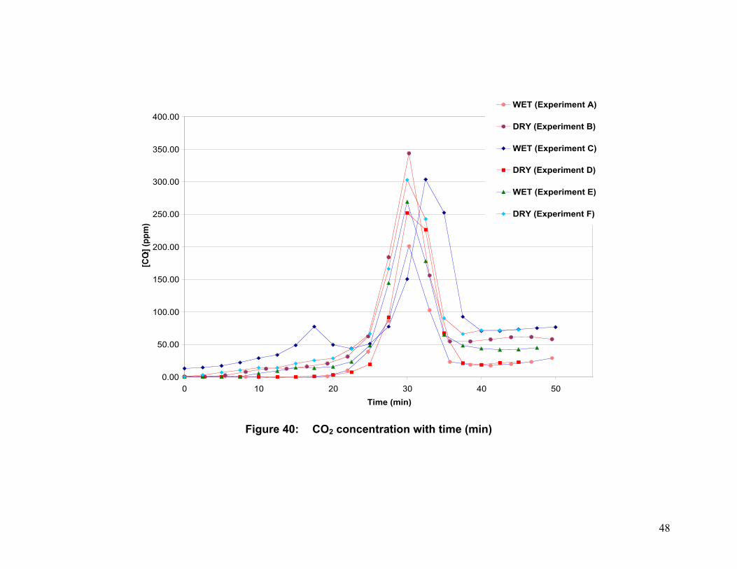
APPENDIX B: TGA GRAPHS GENERATED FOR THE TAGUCHI RUNS 71
APPENDIX C: WORKING PRINCIPLE OF FTIR 86
APPENDIX D: SPECTRUMS OF EXPERIMENT A AND B 91
EXPERIMENT A: .................................................................................................... 91
EXPERIMENT B: .................................................................................................. 101
APPENDIX E: ACTUAL AND PREDICTED DATA OF THE MODEL 111
ATTACHMENT II 116
ATTACHMENT III 119

1
1.0 INTRODUCTION AND OVERVIEW
A typical sintering furnace is divided into three zones. The first zone of asintering furnace is solely used for the removal of lubricants from the compactedpart. This is achieved by heating the part to temperatures in the range of 500-6000C at a controlled rate and atmospheric conditions. The de-lubricated partthen enters the hot zone where it is heated to higher temperatures (close to itsmelting point) for sintering. The third zone or the cooling zone cools the sinteredpart at a desired rate to get the requisite micro structural properties. Proper de-lubrication is an important issue for the following reasons:
1. The end temperature of the first zone is normally 550-600 0C. Figure 1shows a typical temperature furnace profile across the length of the furnace.As the part enters the hot zone (temperatures of 1200-1300 0C), itexperiences a temperature gradient in a very short time, which causes theleft over lubricant to expand rapidly and introduce cracks on the surface(blistering).
2. Improper gas flows and belt speeds can lead to the deposition carbon on thepart. This is called sooting.
3. Most lubricants are hydrocarbons and improper removal can lead to carbonsegregation at the grain boundaries.
Micro-cracks, carbon segregated grain boundaries and sooting are strong qualitydetractors of sintered parts. Very little knowledge base in the various parametersand kinetics of the reactions during de-lubrication has has stymied thedevelopment of effective control systems for this process. Manufacturers followdifferent strategies to alleviate this problem. These vary from longer de-lubrication zones to increased amount of moisture in the furnace.
The literature review and the plant visits we carried out have confirmed that thephysics of de-lubrication are not well established and the reason why thereexists so many approaches. The objective of this work is to understand thephysics of de-lubrication, and based on this knowledge, to recommend a controlstrategy.

2
Figure 1: Typical temperature profile in a furnace

3
1.1 Organization of Work
According to this objective, i.e., to understand the de-lubrication process and todevelop control systems for effective de-lubrication we subdivided the projectin three phases.
Phase 1: Ascertain the most important parameters that affect the kinetics ofde-lubrication.
Phase 2: Investigate the type of gases released during de-lubrication. This isrequired to control the process.
Phase 3: Recommend a control strategy.
2.0 LITERATURE REVIEW
The critical literature review is divided into three sections. Section 2.1 addressesthe need of lubrication in sintering. Section 2.2 gives the properties required in alubricant and lists some of the most common lubricants used in the industry.Section 2.3 presents the various key parameters, which affect the removal oflubricants.
2.1 Need For Lubrication
All powder metallurgical parts are compacted to get the desired shape and greendensity prior to sintering. During the process of compaction, the powder issubjected to enormous pressures as the powder is pressed in a die to achievethe required green density. The frictional forces can be categorized as: Thefriction between the powder particles as they flow with increasing pressure.
1. The friction between the die wall and the powder as the powder iscompacted.
2. The frictional forces generated when the compacted part is ejectedfrom the die.
The frictional forces between the powder particles deter achievable higher anduniform density. Frictional forces between the walls and the powder reduce dielife. These disadvantages are alleviated by the use of lubricants duringcompaction.
Lubrication is normally achieved by die wall lubrication or powder lubrication. Diewall lubrication is preferred in theory, but is not easy to incorporate into the

4
compaction equipment. Thus, lubricants are usually mixed with the metal powderbefore pressing. Typical concentrations of added lubricants vary between 0.5and 1.5 % by weight.
2.1.1 Effect of Lubrication
Lubricants reduce frictional forces between the powder particles and between thepowder particles and die wall by forming a thin layer of liquid on the surface [1].When appropriately admixed with the powder, lubricants also help increase thegreen density of the component. Figure 2 shows the effect of powder lubricationon the green properties of pressed iron.
Figure 2: Green density as a function of % lubricant & compactionpressure [1]
Though the gain in green density is not appreciable, the ejection force necessaryto remove the compact from the die decreases exponentially with the addition oflubricants. Figure 3 shows the ejection force as a function of the amount oflubricant.
The lowering of ejection pressure after compaction has made the addition oflubricants during compaction attractive. Lower ejection pressure also ensuresthe integrity of the compacted part as it is ejected out of the die [1].

5
Figure 3: Ejection force as a function of % lubricant [1]
2.2 Properties Required In a Lubricant
Addition of lubricant ensures lower friction between the die walls and duringejection by forming a thick film of high viscosity polymer on the particle surface.During compaction, the powder is subjected to enormous pressures. These highcompaction pressures require lubricants with high viscosity; low viscosity fluidsare forced away from the friction points under high pressures. Another importantrequirement is the ease of removal during sintering. Some of the commonlubricants, used commercially are given in Table I.
Table I. Melting ranges and 50% decomposition temperatures forcommon lubricants
Material Melting Range, 0C T1/2 ,0C
Linear Polyethylene 95 — 115 390 — 405
Ethylene Bi-Stearate 135 — 145 410 — 435
Zinc Stearate 115 — 125 440 — 460
Zinc Stearate has been used in the powder metallurgical industry for manyyears; however there have been some recent developments and an interest inmoving away from zinc stearate since the latter decomposes during sintering intovolatile zinc compounds. In addition, tougher environment laws and theavailability of cheap lubricant such as ethylene bi-stearate, has forced industriesto shift to ethylene bi-stearate (Industrial name Acrawax ).

6
2.2.1 Structure and Thermal Decomposition of Ethylene Bi-Stearate
Ethylene Bi-stearate has 76H, 38C, 2O and 2N molecules in its molecule. Theschematic diagram of its molecular chain is shown in Figure 4.
Figure 4: Schematic of EBS molecule
The most interesting aspect of EBS lies in its varying bond strength. The bondstrengths in its molecules range from 78 kcal to 130-kcal [2]. The weakest bondsare the C-N bonds, which are the bonds that break first. The next strongestbonds are the C-C bonds in the center followed by the C-H, and finally thestrongest bonds are the C=O bonds which break the last. The continual thermaldecomposition of the Acrawax lubricant was shown by DTA analysis carried outby Harb Nayar and George White [2]. Figure 5 shows the results of their DTAanalysis. The DTA analysis shows 4 endothermic and 1 exothermic peak. Threeof the four endothermic peaks are below 200 0C, while the exothermic peak is atthe 550-600 0C. The authors concluded that the endothermic peaks areassociated with melting of EBS and the other constituents, which are added inthe manufacturing of EBS. The exothermic peak is the point where the strongbonds (here, C=0 bonds) break away to ethylene, CO and CO2.
Figure 5: DTA analysis of EBS [2]

7
However, most industries have an atmosphere of hydrogen and moisture in thede-lubrication zone. Understanding the decomposition of this molecule in thepresence of moisture and hydrogen will aid the understanding of its thermaldecomposition.
2.3 Parameters Affecting De-Lubrication
2.3.1 Rate of Heating
De-Lubrication is the process of thermal decomposition of the higher molecularweight hydrocarbon under controlled conditions. Heating rate or the rate of heatsupplied affects the decomposition kinetics of the lubricant. If the heating rate isvery high it leads to a very rapid decomposition of the lubricant and theassociated volume change introduces micro-cracks in the parts. Thedecomposition of a large chain varies from one polymer to another. Poly-vinylalcohol decomposes by side chain group elimination; polyacetal requires areactive atmosphere to break up; paraffin wax decomposes by oxidation, etc. [3].The difference is due to chemical bonding and the structure of the polymer [4].Work done by J. Woodthorpe et al [5] has shown that the final weight loss showsno correlation to defect formation. However, slope of the weight loss curve givesa very good indication about the type of lubricant to be used for easy removal.They concluded that lubricants, which decompose into small chains, are easier toremove. The slope of the decomposition curve changes by varying the heatingrate.
DTA analyses done by Harb Nayar & George White [2] on EBS indicate that thebreakdown of the Lubricant occurs in successive steps of endothermic reactionsfollowed by an exothermic reaction [Figure 5]. The kinetics of the decompositionis complex, as EBS breaks into smaller hydrocarbons throughout the heatingcycle. The kinetics of decomposition, to smaller and more thermally stablehydrocarbons, will depend on the amount of energy supplied.
2.3.2 Flow Rate of Gases
The sequence of events that lead to lubricant removal is melting, vaporformation, vapor diffusion through the pores and finally the lubricant vapor beingswept away by the gases in the furnace. The most common problem during de-lubrication due to improper atmospheric conditions and gas flow rates isSooting . Sooting is the deposition of carbonaceous material from the lubricanton the part surface. Sooting is also associated with the migration of de-lubrication products into the sintering zone of the furnace, insufficient gas flowand down draughts in the exhaust stacks of the de-lubrication zone. The meltingpoints and vaporization temperatures of lubricants vary greatly according to their

8
composition. For example, Acrawax and the organic part of Zinc Stearate can beremoved by the time the part temperature reaches 550 0C. If there is a stagnantgas layer on the part it can lead to de-caburization defects [6]. It has also beenshown that C/H ratio and oxygen are critical in the formation of soot [7]. Analysisdone by Colllen and Samrasekera [6] has shown the linear dependence of gasvelocity on the mass transfer phenomena. As the thermal pyrolysis of lubricantsare very rapid, insufficient gas flows lead to a stagnant layer of the lubricantvapor on the part which increase the localized C/H ratio to greater than 1. Thisleads to sooting or deposition of C on the surface of the part. The H to C ratio ina molecule determines the tendency of a hydrocarbon to generate soot . EBShas an inherent disadvantage because it has an H to C ratio of 2, whereascleaner hydrocarbons generally have an H to C ratio of 4 [8]. The tendency toform soot is therefore more prevalent in EBS. Controlling the gas flow duringsintering is therefore essential.
2.3.3 Green Density
The amount of compaction pressure determines the green density of a part. Thegreen density is an indication of the internal porosity in part. As discussed in theprevious section, one of the steps in lubricant removal is its diffusion trough theseinternal pores to the surface. As the pressure for densification is increased thenumber of pores on the surface shows a dramatic decrease [9]. Auborn andJoon have also shown that the top surfaces contain more porosity compared toside surfaces. This was attributed to the smearing of the side surface as the partwas ejected from the die. There was an observed delay in the start of de-lubricant at higher green densities. This was due to the reduced porosity in ahigher green porosity. Figure 6 clearly shows that there is a change in the de-lubrication profile once the compaction pressures are increased. Increasingcompaction pressures in Figure 6 shows a reduction in the internal and externalporosity (for smearing ). There seems to be a delay in the temperature at whichthe lubricant first escapes by more than 500C. The slopes of the curve show adramatic difference with higher compaction pressures. The relationship shown inFigure 6 clearly explains the effect of porosity on the migration of lubricant to thesurface.

9
Figure 6: Effect of compaction pressure on de-lubrication [9]
2.3.4 Atmospheric Conditions
As the lubricant vaporizes and migrates to the surface, presence of oxidizingatmospheres help in cracking up the hydrocarbon molecule. Three types ofgases are used to achieve this end. They are oxygen, carbon dioxide and watervapor. Most powder metallurgical industries have shifted to the use of watervapor for cost, hazards of oxygen, and a low oxidizing potential of carbondioxide. Studies done in this field have shown conflicting results. Studies carriedout by Renowden and Pourtalet [10] have shown that de-lubrication is mostlyunaffected by the use of moisture. Their experiments showed that hydrogenaffects the process of lubricant breakdown. They concluded that Hydrogenbreaks down the hydrocarbon by diffusing into the product and at the same timereduce the oxides. Studies done by George White, Antony Griffo and HarbNayar [11] on the effect of atmosphere showed that the addition of water vaporwith hydrogen had the greatest increase in efficiency.

10
3.0 PHASE Ι: EFFECT OF VARIOUS PARAMETERS ON DE-LUBRICATION
In Phase 1, our goal is to determine the most important parameter affecting thekinetics of de-lubrication. Previous researchers have shown that the parametersaffecting the process of de-lubrication are the rate of heating, molecularstructure, green density, atmospheric composition and the flow rate of gases.Typically work on de-lubrication involves the measurement of weight loss as theselected lubricant is heated. A typical weight loss curve as a function oftemperature is shown in Figure 7.
33850
33900
33950
34000
34050
34100
34150
34200
34250
0 100 200 300 400 500 600 700
Temperature ( C )
Wei
ght
Density : 6.80 gm/cc
Heating Rate : 10 oC/min% Hydrogen : 5Moisture : NilFlow Rate : 40 ml/min
Figure 7: Typical weight loss curve of EBS
Researchers have used the TGA machine (see Appendix A) for thedetermination of lubricant removal. As the weight losses are minute, the TGAmachine with a resolution of 10-6 gm provides good accuracy. As the bulk of thework has been done in ferrous systems, the weight loss curve also incorporatesin it the weight loss due to the reduction of iron oxide by hydrogen. The actualweight loss of the lubricant is obtained by subtracting the weight loss due to FeOreduction, from the total weight loss. The potential flaw with this approach is thatone is assuming a fixed volume of iron oxide reduced( in this case, 0.2 - 0.3 % ofthe total weight of the sample) during the TGA run. However, this is not always afixed amount, and in the analysis of the results, this should be taken inconsideration.
Other researchers have alleviated this problem by measuring the weight loss ofonly EBS. This again simplifies the process of de-lubrication, as one of the main

11
factors affecting the smooth removal of lubricants is the availability of openchannels/pores in the compact. In order to eliminate this subtraction of weightsand to simulate industrial conditions, we instead focused on the slope of thecurve (dW/dT), or the rate of change in weight with temperature. Such anapproach eliminates the calculation of weight losses due to the presence ofhydrogen.
The Taguchi analysis was utilized to determine the role of the key processparameters on the kinetics of de-lubrication. The details of our experimentalplans and procedures are discussed in section 3.1.
3.1 Experimental Plan And Procedure
3.1.1 Experimental Design and Control
The parameters selected are heating rate, % hydrogen, moisture and gas flow.Most TGA samples are in the 1 — 2 gm range; however the surface to volumeratio in such samples do not simulate industrial conditions. Accordingly, we usedlarger samples, 35 — 37 gm. TRS bars of dimensions _ square base and height1 _ were used. This allowed us to have weights ranging from 35-37 gm persample (depending on the green density). The capability of the TGA machine atWPI (which can take weights as high as 100 gms) has permitted the evaluationof such large samples. We limited our experiments to compacts of Fe-0.8%C.Three levels for each parameter were selected. The experimental variables andtheir levels are shown inTable II. The levels were selected so that the middle level, here LEVEL # 2simulates industrial operations. The flow rates were however limited due to theconstraints of the TGA machine. The maximum permissible flow rate in this TGAmachine is 100 ml/min. The amount of lubricant added to all the samples was1% by weight.
Table II. Experimental variables and levels
VARIABLE LEVEL # 1 LEVEL # 2 LEVEL # 3Heating Rate (0C/min) 10 20 30
% Hydrogen 5 15 30Moisture - Low High
Flow Rate (ml/cc) 40 60 80
The samples were prepared in cooperation with Mr. Fred Semel of HoeganaesCorporation. Taguchi L9 matrix was used for the experiments. The experimentalconditions followed are shown in. Table III.

12
Table III. Taguchi matrix to determine the rate of de-lube
FactorsRunTrial * Heating rate
(0C/min)% H2 Moisture Flow rate
(ml/min)1 10 5 - 402 10 15 Low 603 10 30 High 804 20 5 Low 805 20 15 High 406 20 30 - 607 30 5 High 608 30 15 - 809 30 30 Low 40
* The experimental conditions given for each run trial, was carried three times(foreach density 6.8 gm/cc, 6.95gm/cc and 7.04 gm/cc). Due to the dependence ofde-lubrication on green density, an L9 matrix was used for 3 different densities6.8 gm/cc, 6.95 gm/cc and 7.04 gm/cc (27 trial runs all together). This was doneto examine the delay in the lubrication burnout for the higher densities. Theprimary gas used in the experiments was nitrogen. The composition of theatmosphere was controlled by controlling the flow rate of gases. For example,for a flow rate of 80 ml/min and a required hydrogen composition of 5%,hydrogen was controlled at 4 ml/min, the reminder (76 ml/min) being nitrogen.The amount of moisture was controlled by passing nitrogen through a sealedwater bath. For low amounts of moisture, nitrogen was passed through water atroom temperature. For high moisture, nitrogen gas was passed through the bathof boiling water held at 80-85 0C. To prevent condensation of water before itentered the TGA furnace, the tubes were pre-heated.
3.1.2 Experiments to determine the decomposition kinetics of EBS
The TGA (see Appendix A) allows one to heat a sample and progressivelymeasure the change in weight of the sample. Using this apparatus, samples of_ square base and 1 _ height were put in the atmosphere dictated by the L9Taguchi matrix. All the samples have the same composition Fe-0.8% C with 1%lubricant (EBS).
The samples were placed in the crucible, which hung from end of the TGAbalance. The furnace cover was then brought up around the hanging cruciblesuch that it completely surrounds the crucible. This also ensured an airtightcompartment for atmosphere control. The final temperature of all the sampleswas fixed at 700 0C. The detailed furnace method is shown in.Table IV.

13
Table IV. Method used for heating rates of 100C/min
ScheduleSegment
sRate
(0C/min)Temp(0C)
Time(h:m:s) Helium Nitrogen Hydrogen
DataSave
1 0 25 0:01:0 On On On On2 10 700 01:07:30 On On On On3 -20 25 0:33:30 On On Off Off
The sampling interval was 8 s, i.e., data was collected by the software every 8 s.The flow of Hydrogen gas was put off as soon the temperature reached 700 0Cfor safety reasons.
The weight loss curves of the raw data are given in Appendix B. The onset of de-lubrication, end of de-lubrication and the slope of the weight loss curve wereobtained from the data analysis software provide by the TGA. The data obtainedfrom these experiments are profiled by curves similar to the one shown in Figure7. The critical information obtained from the TGA data are: Start temperature,Onset temperature, Slope (dW/dt), Final temperature, End temperature; theseare shown pictorially in Figure 8.
33850
33900
33950
34000
34050
34100
34150
34200
34250
0 100 200 300 400 500 600 700
Temperature ( C )
Wei
gh
t
Density : 6.80 gm/cc
Heating Rate : 10 oC/min% Hydrogen : 5
Moisture : NilFlow Rate : 40 ml/min
Start Temperature
End Temperature Slope
Final Temperature
Onset temperature
Figure 8: Data obtained from TGA

14
The TGA software identifies these points and prints a report in the form offilename.rpt. Table V shows the values found by the TGA software for trial run 4of the taguchi matrix for green density 6.80 gm/cc.
Table V. Report generated by TGA for a sample of green density 6.80gm/cc and trial run 4 (Taguchi L9 matrix)
Filename : C:\468080.tgd Start Temp : 150 deg C End Temp : 689 deg C Onset Temp : 457 deg C Final Temp : 538 deg C dW/dt : -88.610 mgs/min
In this analysis, an assumption has been made that the reduction of FeO byhydrogen would not affect the slope of the curve. This was verified by evaluatinga control sample of green density 6.95 gm/cc in an atmosphere of 30 %hydrogen and 70 % nitrogen without any lubricant in the sample.The slopes were determined using the software of the TGA. The results areshown in Table VI. It can be seen from this result that our assumption is valid.
Table VI. Report generated by TGA for a sample of green density 6.95gm/cc in 30% hydrogen with no lubricant in the sample
Filename : C:\nl.tgdStart Temp : 23 deg C End Temp: 694 deg COnset Temp : 308 deg C Final Temp: 614 deg CdW/dt : -0.639 mgs/min
The values calculated from the analysis is shown in a tabular form in Table VII -Table IX for each of the densities respectively.
Table VII. Experimental data (6.80 gm/cc)
TrialRun
Rate ofheating(0C/min)
% H2 MoistureGasFlow
(ml/min)Slope
(mgs/min)
OnsetDe-Lube
(0C)
FinalDe-Lube
(0C)˚ ˚ ˚ ˚ ˚ ˚ ˚ ˚
1 10 5 - 40 -38.3 400 4902 10 15 Low 60 -46.4 408 4803 10 30 High 80 -51 408 4754 20 5 Low 80 -88.6 457 5385 20 15 High 40 -91.2 465 5506 20 30 - 60 -60.2 446 5577 30 5 High 60 -121.8 500 5508 30 15 - 80 -72.1 471 6159 30 30 Low 40 -119.9 476 560

15
Table VIII. Experimental data (6.95 gm/cc)
TrialRun
Rate ofheating(0C/min)
% H2 MoistureGasFlow
(ml/min)Slope
(mgs/min)
OnsetDe-Lube
(0C)
FinalDe-Lube
(0C)˚ ˚ ˚ ˚ ˚ ˚ ˚ ˚1 10 5 - 40 -39.1 403 4912 10 15 Low 60 -46.7 412 4803 10 30 High 80 -49 408 4704 20 5 Low 80 -93.9 467 5435 20 15 High 40 -93 471 5486 20 30 - 60 -64.1 450 5607 30 5 High 60 -126.9 519 5808 30 15 - 80 -73.5 468 6079 30 30 Low 40 -121.6 488 575
Table IX. Experimental data (7.04 gm/cc)
TrialRun
Rate ofheating(0C/min)
% H2 MoistureGasFlow
(ml/min)Slope
(mgs/min)
OnsetDe-Lube
(0C)
Final De-Lube
(0C)˚ ˚ ˚ ˚ ˚ ˚ ˚ ˚1 10 5 - 40 -46.3 454 5262 10 15 Low 60 -49.9 415 4823 10 30 High 80 -49.3 410 4794 20 5 Low 80 -96.17 462 5405 20 15 High 40 -95 470 5486 20 30 - 60 -54 436 5627 30 5 High 60 -127.7 512 5988 30 15 - 80 -74.43 478 6199 30 30 Low 40 -124.4 485 574

16
3.2 Results
3.2.1 Quantitative Analysis
The data from the Table VII - Table IX were analyzed using ANOVA (Analysis ofVariance). Percentage contribution on the variance of the slope were calculatedand the results are shown in Table X - Table XII for each of the three densitiesevaluated.
Table X. ANOVA (6.80 gm/cc)
Factors
Degreesof
Freedom
Sum ofSquares Variance
PercentageContribution
Rate of Heating 2 5338.28 2669.14 70.25% Hydrogen 2 254.30 127.15 3.35
Moisture 2 1768.10 884.05 23.27Gas Flow 2 237.91 118.95 3.13
Table XI. ANOVA (6.95 gm/cc)
Factors
Degreesof
Freedom
Sum ofSquares Variance
PercentageContribution
Rate of Heating 2 5954.14 2977.07 71.62% Hydrogen 2 364.24 182.12 4.38
Moisture 2 1761.78 880.89 21.19Gas Flow 2 233.44 116.72 2.81
Table XII. ANOVA (7.04 gm/cc)
Factors
Degreesof
Freedom
Sum ofSquares Variance
PercentageContribution
Rate of Heating 2 5480.60 2740.30 65.06% Hydrogen 2 495.38 247.69 5.88
Moisture 2 2069.99 1035.00 24.57Gas Flow 2 377.48 188.74 4.48

17
The percentage contribution of the processing parameters for each of the threedensities are graphically represented in Figure 9,Figure 10, and Figure 11respectively. The rate of heating is one parameter which stands out as having amajor effect in all three density regimes.
Percentage Contribution of parameters
71%
3%
23%
3%
Rate of HeatingHydrogenMoistureGas Flow
Figure 9: Percentage contribution (green density 6.80 gm/cc)
Percentage Contribution of Parameters
72%
4%
21%3%
Rate of HeatingHydrogenMoistureGas Flow
Figure 10: Percentage contribution (green density 6.95 gm/cc)

18
Percentage Contribution of parameters
65%6%
25%
4%
Rate of HeatingHydrogenMoistureGas Flow
Figure 11: Percentage contribution (green density 7.04 gm/cc)
3.2.2 Qualitative Analysis
Quantitative analysis was carried out to evaluate the effect of key processingparameters on the de-lubrication process. The response of each parameter isthe average of the slopes for each individual level in a given parameter. Forexample, for a green density of 6.80 gm/cc the data obtained (refer to Table VII)was segregated according to the levels. The rate of heating has 3 levels R1, R2and R3. R1 representing 10 0C/Min, R2 20 0C/min, and R3 representing 300C/min. The corresponding slopes for heating rates of 10 0C/min were averaged(in the slopes column Table VII).
R1 = ( -38.3 + -46.4 + -51) / 3 = - 45.23
Similarly, the response was determined for all the levels for each parameter.Figure 12, Figure 13, and Figure 14 show the effect of de-lubricationcharacteristics for the three respective densities.

19
-120
-100
-80
-60
-40
-20
0
R1 R2 R3 H1 H2 H3 M1 M2 M3 G1 G2 G3
Parameters ( levels)
Res
po
nse
Rate of Heating ( Levels)
% Hydrogen (Levels)
Moisture(Levels)
Gas Flow rates(Levels)
Figure 12: Qualitative Effect of parameters (6.80 gm/cc)
-120
-100
-80
-60
-40
-20
0
R1 R2 R3 H1 H2 H3 M1 M2 M3 G1 G2 G3
Parameters ( levels)
Res
po
nse
Rate of Heating ( Levels)
% Hydrogen (Levels)
Moisture(Levels)
Gas Flow rates(Levels)
Figure 13: Qualitative effect of parameters (6.95 gm/cc)

20
-120
-100
-80
-60
-40
-20
0
R1 R2 R3 H1 H2 H3 M1 M2 M3 G1 G2 G3
Parameters ( levels)
Res
po
nse
Rate of Heating ( Levels)
% Hydrogen (Levels)
Moisture(Levels)
Gas Flow rates(Levels)
Figure 14: Qualitative effect of parameters (7.04 gm/cc)
Qualitative analysis shows effect of on the slope or the kinetics of de-lubrication.If the requirement of the system is to have maximum removal in the shortest timeinterval, referring to Figure 12 - Figure 14, one can determine the lowest pointsfor each individual line. For example, to have a maximum slope in Figure 14 weselect the lowest points for each individual parameter line. In this case, they areR3, H1, M3 and G1, which correspond to 30 0C/min, 5% hydrogen, high moistureand low flow rate of gases. For slow removal, the highest points in the curve, i.e.,R1, H2, M1 and G3 determine the optimum condition.
3.3 Discussion
Taguchi analysis has clearly shown that the kinetics of decomposition isessentially a thermal event and that the rate of heating determines the de-composition kinetics. For a control system to evolve and to ensure effective de-lubrication, the rate of heating has to be controlled. The moisture has shown tohave an effect on the de-lubrication kinetics, but controlling the moisture in acontrol system is not desired as it oxidizes the surface of iron samples, andrequire a reducing gas and hydrogen to maintain the balance. Moisture and theflow of gases may be required on the other hand to prevent sooting and the buildup of a stagnant layer on the part. Though higher heating rates remove lubricantsfaster from the part, the faster the better approach might be deleterious to the

21
part. The rate of polymer breakdown to smaller hydrocarbon chains should beless or equal to the rate of removal from the part. Non-equilibrium in the rateswill result in the introduction of cracks in the part.

22
4.0 PHASE ΙΙ : ANALYSIS OF GASES IN DE-LUBRICATION
4.1 Motivation
One of the challenges for a sintering furnace operator is to ensure that, thelubricant in the green part is removed completely before the part enters thesintering zone. Various companies have adapted different techniques to ensurecomplete lubricant removal. Some manufacturers have longer de-lubricationzones while others have introduced moisture into their furnaces. Though, thesede-lube solutions have partly solved the problems, most industries havenumerous questions unanswered; What gases are released during de-lubrication? Does moisture play a role in the decomposition of lubricants? Isthere the possibility to control the process? These questions were partlyanswered by Harb Nayar and George White [2] in 1995. Their study however,did not lay down the mechanism of de-lubrication and failed to conclusivelyidentify the various gases and by-products released during de-lubrication. Theeffect of moisture on de-lubrication was left untouched. Understanding thefundamental reactions and identifying the gaseous by-products formed during de-lubrication is the key to sensor development. The primary motivation for thisphase is to identify various gases released during de-lubrication and to identifythe mechanism of de-lubrication. The results of this study will aid in thedevelopment of future sensors for de-lubrication.
4.2 Chemical Analysis By Spectroscopy
Different forms of radiant energy such as radio waves, sunlight, x-rays etc havesimilar properties, and are called electromagnetic radiation. The radiations aremost commonly classified according to the frequency, ν, the number of wavesthat pass a particular point per unit time. In all electromagnetic waves, thefollowing relation gives the frequency;
Frequency (ν) = (cm) wavelength
(cm/sec)light ofvelocity (1)
Figure 15 shows the schematic diagram of the electromagnetic spectrum.

23
Figure 15: Schematic of electromagnetic spectrum
4.2.1 Absorption of light
When atoms or molecules are subjected to intense heat or electric, they absorbenergy and become excited . One return to their normal state, they emitradiations. The energy lost in the transition is emitted in the form of light.Absorption of light by atoms or molecules is the change from a state of lowenergy to a one of higher energy. According to the Bohr theory, the energychanges in the atom or molecule by light absorption occur in multiples of a unitamount of energy called quanta. The energy changes in a molecule and thefrequency of light emitted or absorbed is given by the so-called Bohr condition:
hν = Ef - Ei ..(2)
Where,h = Planks constantν = FrequencyEf = Final energyEi = Initial energy
Absorption of light leads to three types of changes in a molecule: rotation,rotation — vibration, and electronic. Electronic absorption is a combination ofrotational and vibrational energy.
Rotational energy
The rotational energy of a molecule is associated with changes that occur in therotational states of the molecules. The energies of the various rotational statesdiffer by only a small quantity, hence the energy difference Ef — Ei is a smallnumber. From equation 2 one can conclude that the frequency of light requiredfor this change is small. Hence, changes in pure rotational energies are observedin the far infrared and microwave regions (Figure 15).

24
Rotational — vibration energy
These energy changes are associated with transitions in which the vibrationalstates of the molecule are altered and may accompanied by a change in therotational states. Since the energy difference is greater between the initial andthe final vibrational state is greater than between rotational states, absorptionoccurs in at larger frequencies or shorter wavelength. Therefore the vibration —rotation transition occur in the middle infrared region (refer Figure 15).
Electronic energy
These spectra arise from the transitions from between electronic states andaccompanied by simultaneous changes it the vibration and rotational states.Relatively large energy differences are involved, and hence absorption occurs atlarge frequencies or shorter wavelengths. All electronic transitions occur in theultraviolet and visible region (refer Figure 15)The various energy levels are illustrated by means of a schematic diagram,Figure 16. The dark lines represent the electronic energy levels of two electronicstates. The thin lines (1,2 and, 3) represent the electronic transition when thenuclei of the atoms are held motionless i.e. no vibrational and rotational energy.The series of broken lines in the extreme right represent the various rotationallevels in each electronic state. Transition from A to B is a pure rotational, from Ato C is a combination of rotational vibrational and electronic (involves 1 to 2states) transitions. Excited State (E f)
Initial State (Ei) 1
2
3
A B
C
Figure 16: Energy levels in a molecule
Each electronic state is associated with a large number (nearly infinite) ofvibrational and rotational states. A large number of spectrum lines result fromthese transitions, and these are not widely spaced form one another. Though

25
these lines are of interest to find the rotational translations during absorption,practically all spectroscopy rely on the electronic transitions. Infraredspectroscopy is the study of interaction of the infrared light with matter. Inspectroscopy wave number (W) is most commonly used to describe the energytransitions. Wave number is the reciprocal of wavelength.
Wave number (cm-1) =(cm) Wavelength
1 (3)
The following relation gives energy.
Energy =λhc
(4)
Where;h = Planks Constantc = Speed of lightλ = Wavelength
Substituting equation 3 in equation 4 gives a relation where the energy is directlyproportional to the wavenumber (W) as follows;
Energy = hcW (5)
Thus, high wave number light has a lower energy than low wave number light.When infrared radiations interact with matter it can be absorbed, causing themolecular bonds in the molecule to vibrate (4.2.1). The presence of chemicalbonds is a necessary condition for infrared absorbance to occur. Chemicalstructural fragments within molecules, known as functional groups, tend toabsorb infrared radiation in the same wave number regardless of the structure ofthe rest of the molecule. For instance, the C=O stretch occurs at 1700 cm-1 inketones, aldehydes, and carboxylic acids. This correlation between the wavenumber and the functional group makes infrared spectroscopy a useful chemicaltool.
4.2.2 Laws of light absorption
The two principle laws of light absorption are Bouguer and Lambert s law andBeer s law. Bouguer and Lambert s law states that the proportion of lightabsorbed by a transparent medium is independent of the intensity of the incidentlight. Each successive layer of the medium absorbs an equal fraction of theincident light. This is mathematically represented by the following expression.
Ι = Ιo x e-αb (6)
Where, Ι = Intensity of the light transmittedΙ0 = Intensity of the incident lightα = Absorption coefficient of the medium

26
b = Thickness of the layer
Equation 6 can be represented as
log e (0ΙΙ
) = αbc (7)
When the logarithm of base 10 is used, α is converted to Bunsen and Roscoeextinction, K, and α = 2.303 K.The second important law, Beer s law states that the amount of light absorbed isproportional to the number of absorbing molecule through which the light passes.Light is absorbed due to the collision of photons with the molecule or atoms. Theproportionality to concentration is incorporated into the Bouguer and Lambert slaw to give equation 8.
Ι = Ιo x 10-abc (8)
Where,Ι & Ι0 = Intensity of light transmitted and incidenta = Absorptivity, a molecular propertyb = Cell lengthc = Concentration
The ratio of ΙΙ 0 is usually called the transmittance, and represented by T.
T =ΙΙ 0 (9)
Substituting equation 9 to equation 8 reduces it to a form given by equation 10.
log(Τ1
) = abc (10)
A typical spectrophotometer measures log(Τ1
). It is also called absorbance. The
working principle of a FTIR is detailed in Appendix C. Spectrum obtained withoutthe sample in the infrared beam is called a background spectrum. A typicalbackground spectrum is shown in Figure 17.

27
Figure 17: Typical Background Spectrum
The background spectrum contains the instrument s and the environmentscontribution to the infrared spectrum. Common features around 3500 and 1630cm-1 are due to atmospheric water vapor, and the bands at 2350 and 667 cm-1
are due to carbon dioxide. When a sample is run in the FTIR, a similar spectrumis obtained except that the sample peaks are superimposed upon theinstrumental and atmospheric contributions to the spectrum. The spectrum ofpolystyrene with the background is shown in Figure 18.
Figure 18: Spectrum with sample
To eliminate the environment and atmospheric contribution, a ratio between thesample spectrum (Figure 17) and the background spectrum (Figure 18) isperformed. This produces a transmittance spectrum as shown by Figure 19. Thetransmittance spectrum is represented by equation 11.

28
% Τ =0ΙΙ
(11)
Where,%Τ = TransmittanceΙ = Intensity measured with a sample in the beamΙ0 = Intensity measured with no sample in the beam
Figure 19: The transmittance spectrum (ratio of Figure 17 and Figure 18)
The absorbance spectrum can be obtained from the transmittance spectrumusing the following equation.12
A = log10(Τ1
) (12)
4.3 Experimental Setup And Design
Samples (_ square base and height 1 _ ) containing 1% EBS ( Acrawax ) as thelubricant were heated in a specially designed furnace. The schematic diagram ofthe furnace is shown in
Figure 20. The slot above the sample was designed for the thermocouple. Theatmosphere used in all the experiments had a composition of 95 % Nitrogen +5% Hydrogen. To add moisture to the atmosphere, the mixture of nitrogen andhydrogen was passed through a bubbler. The flow rate of the gases was 2liters/min. The temperature of the bubbler was maintained to the requiredtemperature by heating coils around the bubbler. A schematic of the gasconnections are shown in Figure 21.

29
f
e d
c
b b
a
N2 / H2 Mixture
Moisture
Sample (32 mm x 13 mm sq. base)
40 mm ID Ball &Socket ground glass joint
Material: QuartzDimesions: a 15 mm b 150 mm c 6 mm
d 50 mm e 73 mm f 38 mm
Figure 20: Schematic diagram of the heating furnace

30
.
Cylinder with 95 % Nitrogen + 5 % Hydrogen
Water bath heated by coils
Distributor
Flow Meter
Gas direction valve
Check Valve A
Check Valve B
To Furnace
Figure 21: Schematic diagram of gas flow direction
Check valve A and B prevented the outflow of moisture laden gas back throughthe flow meter in case of pressure build up. The gas direction valve ensuredeither moisture or no moisture into the furnace. The pipes were heated to preventmoisture condensation. The temperature was maintained buy self-heating coils.A schematic of the entire setup is shown in Figure 22.

31
N2/H2 mix
Flow Meter
Water at required temperature
Sample Filter
DUV Spec.
FTIR Check Valve
Figure 22: Schematic diagram of the experimental setup
The actual experimental setup is shown in Figure 23. The following steps werefollowed in all the experiments:
- The entire system was purged with dry nitrogen for 15 minutes.- Background spectrums were collected at random during this initial process
to ensure minimum atmospheric contamination.- The atmosphere for the experiment (N2/H2 mixture + moisture/no
moisture) was then passed for a period of 15 min and allowed to stabilize.- The furnace temperature with the sample was maintained and equilibrated
at 1000C during the entire process of atmospheric control.- The temperature of the gas tubes was maintained by self-heating coils to
temperature above that of the water bath (in wet conditions) to ensure thatthe moisture content remains constant during the collection of spectrums.
- The FTIR cell and the DUV cells were insulated and heated to 1200C toprevent condensation of moisture on the cell windows.
- Once the background spectrums showed minimum contamination, thesample was heated at 100C/min to 6000C.
- The optical path lengths (discussed in detail in Appendix C) weremaintained at 5m for the FTIR and 0.5 m for the DUV.
- FTIR and DUC spectrums were collected every 2.5 minutes.- The flow rate of the gases was maintained at 2 liters/min.

33
Flow Controller
Nitrogen + 4 — 5 % Hydrogen Cylinder
Junction splitting the volume of by-products to DUV and FTIR cells
Temperature controller of the furnace
FTIR cell
T — junction, for wet and dry gas.
Bubbler for wet atmosphere
Furnace DUV cell
Figure 23: Experimental Setup

34
4.3.1 Identification of by-products
Three experiments were performed for a wet atmosphere and three in dryconditions. The experiments were labeled as follows:
A, C and E - WetB, D and F - Dry
FTIR Spectrums
Each experiment consisted of 19 spectrums and a background spectrum. Thespectrums of experiment A (page 90 — 100) and B (page 101— 110) are shown inAppendix D. All the spectrums have wave number in the X — axis andabsorbance in the Y — axis. Similar spectrums were obtained for experiments C —F. The spectrums obtained were studied to identify the by-products releasedduring the decomposition of EBS. The spectrums were analyzed for the variousfunctional groups present in the system. Figure 24 and Figure 25 depict thecharacteristic wave number for the functional groups in hydrocarbon for a rangeof wave number (Figure 24 from 3500 — 1700 cm-1 and Figure 25 from 1700 —700 cm-1) [12].Figure 26 - Figure 30 show the major peaks observed during thedecomposition of EBS. Figure 26- Figure 28 are enlarged from spectrum 14 ofExperiment B (Appendix D, page 106). Figure 29 - Figure 30 are enlarged fromspectrum 14 of Experiment A (Appendix D, page 97).

35
Figure 24: Characteristic group wave numbers of hydrocarbons (3500 - 1700 cm-1)

36
Figure 25: Characteristic group wave numbers of hydrocarbons (1700 — 700 cm-1)

37
2932
2967
2863
2360
Figure 26: Observed peaks between 3000 - 2000 cm-1 (no moisture)
1470 - 1458
1646
Figure 27: Observed peaks between 1800 - 1300 cm-1 (no moisture)

38
912
950 992
Figure 28: Observed peaks below 1000 cm-1 (no moisture)
2933
2863 2360
2873 — 2963
Figure 29: Observed peaks between 3000 - 2300 cm-1 (wet conditions)

39
912
688
798
744 — 740
Figure 30: Peaks below 1000 cm-1 (wet conditions)
DUV spectrums
Spectrums obtained in the deep ultraviolet spectroscopy are displayed in Figure31 - Figure 32. The spectrums clearly show the presence of Ammonia as the by-product. Figure 31 is the spectrum under wet conditions. Figure 32 is thespectrum obtained for dry conditions. The spectrums shown in these figures aretaken at the same time/temperatures as the FTIR spectrums.
Wavelength (nm)
Abs
orba
nce
(AU
)
0
0.01
0.02
0.03
0.04
0.05
0.06
0.07
0.08
0.09
0.1
195 200 205 210 215 220 225 230 235 240
Peaks of
Ammonia
Figure 31: Spectrum in DUV under wet conditions

40
Abs
orba
nce
(AU
)
0
0.05
0.1
0.15
0.2
0.25
0.3
0.35
0.4
0.45
0.5
195 200 205 210 215 220 225 230 235 240
Wavelength (nm)
Peaks of Ammonia
Figure 32: Spectrum in DUV under dry conditions
Table XIII shows the various functional groups identified form the spectrums.

41
Table XIII. Functional groups in the FTIR spectrums
DRY ATMOSPHEREWave Number
(cm-1)Functional Group Theoretical Values
3085, 3015 Stretch of unsaturated CH 3080 and 30202965, 2863 Stretching of Methyl (-CH3) 2960 and 28702932, 2855 Stretching of Methylene (-CH2-) 2925 and 2850
2360 O = C =O 2349C = C stretch 1640
Terminal Methylene stretch in R/CH = CH2 16451646C = C stretch of terminal Methylene 1655
1470 - 1458 Methylene and methyl bending 1470 and 1460992, 912 Out of plane δCH of terminal vinyl 990 and 910
966 Out of plane δCH of trans double bond 965WET ATMOSPHERE
Wave Number(cm-1)
Functional Group Theoretical Values
2967, 2863 Stretching of Methyl (-CH3) 2960 and 28702933 Stretching of Methylene (=CH2) 2925 and 28502360 O = C =O 2349
1646 Water Interference
1470 - 1458 Water Interference992, 910 Out of plane δCH of terminal vinyl 990 and 910
966 Out of plane δCH of trans double bond 965798 Rocking of -CH3 = CH2 780
744 - 740Doublet of (CH2)n where n > 4, Higher with lower
’n’ 725 — 720
The primary by-products can be readily inferred form Table I:
• A long chain hydrocarbon (due to - CH3, -CH2-)• Carbon Dioxide• Ammonia (from the DUV unit)• Carbon Mono-oxide
To identify the hydrocarbon released during the decomposition of EBS, a sampleof the solid phase was collected on a KBr disc and observed in the FTIR Figure33 shows the spectrum obtained from the FTIR analysis.

42
0
10
20
30
40
50
60
70
80
90
100
940114013401540174019402140234025402740294031403340354037403940
Wavenumber (cm-1)
Tran
smis
sion
(%)
Figure 33: Spectrum of the solid by-product (hydrocarbon)
The hydrocarbon was identified as heptadecane. Figure 34 is the spectrum ofheptadecane from NIST.
Figure 34: Heptadecane spectrum from NIST

43
4.3.2 Quantitative Analysis
As stated in section 4.2.2, the spectrum obtained from the FTIR can be used todetermine the concentration of the products obtained. Theoretically, the value ofa in equation 10 is a unique function of the component in question (at thefrequency for which it is determined). A plot of absorbance and concentrationshould be a straight line. However, in practice a is dependent on the operatingconditions, and it introduces non-linearity into the equation. This is taken care bycalibrating the instrument with products of known concentration over the requiredrange. Known concentrations of gases are passed through the instrument andthe actual and observed values are compared. Figure 35 - Figure 36 show theobserved and actual concentrations of CO2 and NH3 during calibration. All thecalibrations were performed in the same operating conditions and gas flow ratesas the actual experiments.
y = 0.000479x2 + 1.063333xR2 = 0.999121
0.0
200.0
400.0
600.0
800.0
1000.0
1200.0
0.0 100.0 200.0 300.0 400.0 500.0 600.0 700.0 800.0
Observed (ppm)
Act
ual
(ppm
)
Figure 35: Calibration curve of actual and observed concentrations ofCO2 (pm)

44
NH3 Calibration
y = -0.001804x2 + 1.062906xR2 = 0.999478
0.0
10.0
20.0
30.0
40.0
50.0
60.0
70.0
80.0
90.0
0.0 10.0 20.0 30.0 40.0 50.0 60.0 70.0 80.0 90.0 100.0
Observed (ppm)
Act
ual (
ppm
)
Figure 36: Calibration curve of Ammonia
The smaller concentrations of CO involved in the experiments signify a linearrelation in the range of interest. As heptadecane cylinders of knownconcentrations are not manufactured, the concentration is reported as a ratio of amost readily available hydrocarbon. In this study, the concentrations ofheptadecane are compared to propane. A calibration curve of propane wasobtained. Figure 37 shows the calibration curve of propane. Figure 38 shows thespectrums of the hydrocarbon and propane of known concentration. A factor wasidentified which would give the closest match to the hydrocarbon peaks. Thisfactor was utilized to report the hydrocarbon concentration.

45
y = -0.000058x2 + 1.033685xR2 = 0.999825
0.0
200.0
400.0
600.0
800.0
1,000.0
1,200.0
1,400.0
0.0 200.0 400.0 600.0 800.0 1,000.0 1,200.0 1,400.0
Observed (ppm)
Act
ual (
ppm
)
Figure 37: Calibration curve of propane
0.00000
0.10000
0.20000
0.30000
0.40000
0.50000
0.60000
0.70000
0.80000
2800 2850 2900 2950 3000 3050 3100 3150 3200 3250
Wave number
Abs
orba
nce
Figure 38: Hydrocarbon (dark) and propane (dotted) spectrum

46
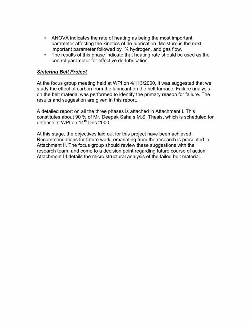
The concentrations in the experiments with the experimental samples wereobtained using Beer Lambert s equation (equation 10). The concentrations werethen corrected using the calibrated curves shown in Figure 35 - Figure 37. Forexample, Table XIV shows the raw data (2nd column) obtained from the FTIR.The actual CO2 concentrations were obtained by using the calibration equationon Figure 35. The concentration of CO2 with time is shown in Figure 40.
Table XIV. Raw and calibrated data for CO2 (Experiment A)
Time (min) Raw Calibrated0 13.0659 0.921099191
2.75 12.7196 0.5526371495.5 12.9641 0.812772409
8.25 12.2746 0.07932730811 11.461 -0.785541495
13.75 11.3022 -0.95427427216.5 11.2312 -1.029707434
19.25 12.941 0.78819276322 21.3628 9.783322969
24.75 47.9823 38.6617990727.5 90.4783 86.17096836
30.25 187.323 200.904068233 104.637 102.3841754
35.75 33.7232 23.1082246838.5 29.3762 18.40533574
41.25 28.5281 17.4899122444 30.4542 19.56990363
46.75 33.8579 23.2542417449.5 38.9001 28.7325743
Similar calculation was performed for the other identified by-products; theconcentrations of CO, hydrocarbon (as propane) and NH3 are shown in Figure39, Figure 41,and Figure 42 respectively.

47
0.00
5.00
10.00
15.00
20.00
25.00
0 10 20 30 40 50
Time (min)
[CO
] (pp
m)
WET (Experiment A)
DRY (Experient B)
WET (Experiment C)
DRY (Experiment D)
WET (Experiment E)
DRY (Experiment F)
Figure 39: CO concentration with time (min)
48
0.00
50.00
100.00
150.00
200.00
250.00
300.00
350.00
400.00
0 10 20 30 40 50
Time (min)
[CO2
] (pp
m)
WET (Experiment A)
DRY (Experiment B)
WET (Experiment C)
DRY (Experiment D)
WET (Experiment E)
DRY (Experiment F)
Figure 40: CO2 concentration with time (min)

49
0.00
100.00
200.00
300.00
400.00
500.00
600.00
700.00
800.00
900.00
0 10 20 30 40 50
Time (min)
[HC
] (pp
m)
WET (Experiment A)
DRY (Experiment B)
WET (Experiment C)
DRY (Experiment D)
WET (Experiment E)
DRY (Experiment F)
Figure 41: Hydrocarbon concentration (as propane) vs time (min)

50
0.00
5.00
10.00
15.00
20.00
25.00
0 10 20 30 40 50
Time (min)
[NH
3 ] (p
pm)
WET (Experiment A)
DRY (Experiment B)
WET (Experiment C)
DRY (Experiment D)
WET (Experiment E)
DRY (Experiment F)
Figure 42: Ammonia concentration with time (min)

51
4.4 Conclusions
The primary gases identified during the decomposition of EBS are carbondioxide, carbon monoxide, ammonia and a heavy hydrocarbon (heptadecane).The experiments involved are from a part with 1%lubricant (EBS) in them. Themaximum concentration detected for the various identified gases are listed asfollows:
Carbon Monoxide - 19 ppmCarbon dioxide - 350 ppmAmmonia - 22 ppmHeptadecane - 850 ppm
Development of sensor to detect the changes in concentration would require thedetection of CO2 and heptadecane. A typical furnace has a load varying from 150lb/hr — 1000 lb/hr. The concentrations listed above are for a single part of weight35 gm. The concentration of gases under industrial conditions should be an orderof magnitude higher.

52
5.0 PHASE ΙΙΙ : MATHEMATICAL MODEL FOR DE-LUBRICATION
5.1 Introduction
De-lubrication is the first stage in a typical sintering operation where, the lubricantin a compacted part is removed by controlled heating and atmosphericconditions. Previous researchers have shown the effect of various parameters onthe kinetics of de-lubrication [13,14,15,16]. The important parameters, whichneed to be considered, are heating rate, moisture content, hydrogen and the flowrate of the gases. However, an understanding of this process is complete onlywhen the process is well described by a mathematical function, whichincorporates in it, all the parameters involved. To control the de-lubricationprocess a quantitative (not qualitative) understanding and a functionalrelationship of the process parameters. Such knowledge enables are to predictand control the process on-line. De-lubrication is a combination of two processes:
1. The thermal degradation of the polymer to smaller hydrocarbons.2. The transfer of the polymer/degraded molecules from the part to the
atmosphere.
The kinetics of degradation of any polymer is given by the following equation:
)exp()1(RT
EA
dtd n −−= αα
(13)
Where;α = Weight fraction of polymerA = Pre-exponential factor (1/min)E = Activation energy (J/mol)R = Gas Constant (8.314 J/mol K)T = Temperature (K)n = reaction order
The values of n , A and E vary with the amount of energy supplied. Theenergy supplied is directly dependent on the applicable heating rate. If theconstants n , A and E are known for a heating rate, the process is fullydescribed. However, the additional variables in powder metallurgical applicationssuch as green density, % hydrogen and moisture, make the exact mapping of n,A and E with temperature quite complex. To describe the processmathematically with the objective of having a workable model for de-lubrication,we have taken two parallel approaches:

53
1. Evaluate the average activation energies (E), A and n as described inequation or various conditions during de-lubrication.
2. Formulate an empirical predictive model for the process of de-lubrication,which is empirically based.
5.2 Theoretical Model Of De-Lubrication
Experiments on polymers are performed on a Thermo-gravimetric analysismachine (TGA), which determines the weight loss of the lubricant as a function oftime / temperature. Thermo-gravimetric analysis can be used to provideinformation regarding the activation energy and the overall reaction order [17 -20]. A typical TGA curve is shown in Figure 43. However, deducing preciseinformation on the kinetics of polymer breakdown cannot be obtained from TGAdata because the reaction order (n) is not known. Most researchers assumed afirst order reaction (n = 1), which remains a good approximation [21].
33850
33900
33950
34000
34050
34100
34150
34200
34250
0 100 200 300 400 500 600 700
Temperature ( OC )
Wei
ght (
mgs
)
Heating Rate : 10 oC/min
Figure 43: Typical weight loss curve
Mathematical analysis of equation (14) performed by Kyong Ok Yoo et al [22]has shown that the plot of Ln(Rate of heating) and 1/Tmax should be a straightline. Tmax is the temperature on the curve where the rate of weight loss is the
maximum (point of inflection on the TG-curve / 02
2
=∂∂
t
α ). Figure 44 illustrates the
inflection point. The following data can be inferred form the curve of 1/Tmax andLn(Rate of Heating):
Slope = —E/R
Intercept = ln(A0)+ (2
3)*ln(Tmax)- ln (
RT
E+
2
1)

54
33850
33900
33950
34000
34050
34100
34150
34200
34250
0 100 200 300 400 500 600 700
Temperature ( C )
Wei
gh
t
Density : 6.80 gm/cc
Heating Rate : 10 oC/min% Hydrogen : 5
Moisture : Nil
Flow Rate : 40 ml/min
(Tmax, C)
Tmax
Figure 44: Inflection point and lubricant weight at the point of inflection
5.2.1 Experimental Work
To determine the kinetic parameters of de-lubrication during the process ofsintering, TGA was performed with samples containing 1% acrawax (EBS). Allthe samples were compacted to densities ranging from 6.80 — 7.04 gm/cc. OnlyFe-0.8%C compacted powders were considered for analysis. Historically,equation (1) has been used in the study for the degradation of pure polymers.The activation energies would vary in a compacted part, compared to that of apure lubricant, as the presence of metal can alter the reaction kinetics. To have amodel, that predicts the breakdown of lubricant in a furnace, necessitates the useof metallic compacts. The compacts had the following dimensions: 1/2 squarebase and 11/4 height. Experiments were conducted in the presence andabsence of moisture. Figure 45 - Figure 46 show the plot of Ln (Rate of Heating)and 1/Tmax for the two conditions, without moisture and with moisture.

55
No Moisture
y = -4958.7x + 5.2297
R2 = 0.9512
-2
-1.5
-1
-0.5
0
0.0011 0.00115
0.0012 0.00125
0.0013 0.00135
0.0014 0.00145
0.0015
1/Tmax
Ln
(Rat
e o
f H
eati
ng
)
Figure 45: ln(heating rate) Vs 1/Tmax in dry conditions
Moisture
y = -4780.1x + 4.9606
R2 = 0.9415
-2.5
-2
-1.5
-1
-0.5
0
0.0011 0.00115
0.0012 0.00125
0.0013 0.00135
0.0014 0.00145
0.0015
1/Tmax
Ln
(Rat
e o
f H
eati
ng
)
Figure 46: ln(heating rate) Vs 1/Tmax in wet conditions

56
5.2.2 Results
The values of A0 and E calculated from the data of Figure 45 - Figure 46 areshown in Table XV.
Table XV. ’A0’ and ’E’ for EBS at the point of inflection
No Moisture (Nitrogen) MoistureRate of Heating
(0C/min)A0
(1/min)E (kJ/mol) A0
(1/min)E (kJ/mol)
10 1.0067 0.913820 1.0577 0.961030 1.0929
41.2290.9938
39.743
Table I clearly shows that there is a slight decrease in the activation energy ofde-lubrication when moisture is added to the system. However, these values of E
and A are at the point of inflection ( 02
2
=∂∂
t
α ). The order of reaction (n) varies over
the entire range of decomposition. According to Denq et al [20], thermaldegradation by zero-order reaction order indicates that the molecular chainbreaks by monomer scission at the chain end. Thermal degradation by first-orderreaction indicates weight loss by the random scission of the main chain [19]. Asecond order reaction order would indicate intermolecular transfer and randomscission. FTIR (Fourier Transform Spectrometer) analysis performed by HarbNayar and George White [21] shows the presence of monomer units (-CH3, -CH2-) in the by-product during the initial period of de-lubrication followed by thepresence of large hydrocarbon molecules at higher temperatures. EBS molecule(shown in Figure 47) shows that the —CH3 group is positioned at the ends of thepolymer chain. This indicates that the decomposition of EBS proceeds by thescission at the polymeric ends (-CH3) and at the center (-CH2-). This implies afirst order reaction order.
Figure 47: Molecular structure of EBS

57
5.2.3 Conclusions
The kinetic model shows that moisture reduces the activation energy required forthermal degradation. The decrease in energy is however negligible (@E = 1.484KJ/mol). The same model can be used to determine the affect of alloyingelements (Ni, Cu, etc in the compact) on de-lubrication. The drawback of thisanalysis is the determination of n during degradation. Though the average valueof n can be considered equal to unity, the value of n changes as thedecomposition changes from the scission of —CH3 / —CH2- monomer units toother random units. Moreover, the activation energy determined from this modelis the energy at the point of inflection. Realistically, the value of E changes as themode of scission changes from one monomer unit to another. The change in thevalues of n and E with time only complicates the mathematical model, as moreapproximations are made to mathematically solve the problem.
5.3 Empirical Model For De-Lubrication
The kinetic model explained in the earlier section clearly explains the underlyingthermal kinetics. In this section we determine an empirical model for de-lubrication by curve fitting techniques. De-lubrication curves obtained from theexperiments in the previous section were analyzed to determine a mathematicalfunction. The de-lubrication curve can be described as shown in equation 14.
b
tt
)(1
1
max
+=α
(14)
Where,
α = 0W
Wt (Weight fraction at any time t )
W0 = Initial weight of the lubricant
Wt = Weight of the lubricant at any time t
t = Time
tmax = Time at the point of inflection (Max. slope of the curve)
b = Constant depending on the conditions

58
The boundary conditions governing the equation are: t = 0, α =1 and t = infinite, α= 0. Appendix E shows the actual Vs the predicted data (-Pr). The values of band tmax ( c in the graphs) appear at the right hand top corner. Table XVIsummarizes the values of b and tmax for all the experiments.
Table XVI. ’b’ and ’tmax’ for the predicted curves
b tmax (secs) b tmax (secs) b tmax (secs)20.4 2647 23.6 2678 22.57 265120.4 2652 22.2 2593 21.2 2489
23.5 2705 23 268418.2 1484 29.7 1477 35.3 158318.7 1540 31.7 1533 31.3 152515.1 1473 32.7 1563 33.37 157518.5 1132 32.8 1113 33.3 110418.6 1123 34.8 1130 37.8 119018.7 1161 30.9 1073 36 1152
10
20
30
Rate of Heating ( 0C/min)Moisture(High)No Moisture Moisture (Low)
Plots of Ln (rate of heating) and 1/tmax are shown in Figure 48 and Figure 49.Figure 48 shows a plot for the in the absence of moisture, Figure 49 is a similarplot in the presence of moisture.
No Moisture y = 2182.22x - 2.59R2 = 0.99
-2
-1.5
-1
-0.5
0
0.00035 0.00045 0.00055 0.00065 0.00075 0.00085
1/tmax
Ln
(Rat
e o
f H
eati
ng
)
Figure 48: ln(rate of heating Vs 1/tmax (dry condition)

59
Moisture (Low and High) y = 2207.88x - 2.60R2 = 0.98
-2
-1.5
-1
-0.5
0
0.00035 0.00045 0.00055 0.00065 0.00075 0.00085
1/tmax
Ln
(Rat
e o
f H
eati
ng
)
Figure 49: ln(rate of heating) Vs 1/tmax (wet conditions)
Figure 50 shows the plot of b for various atmospheric conditions and the rate ofheating.
’b’ Vs Heating Rate
0
5
10
15
20
25
30
35
40
0 5 10 15 20 25 30 35
Heating Rate (C/min)
b
INCREASING MOISTURE CONTENT
Figure 50: ’b’ Vs rate of heating

60
5.4 Industrial Validation of the Mathematical Model
The proposed mathematical model was applied in furnace to see if there was ananomaly in the model. Ten compacts (Figure 51) of different weights were put ina furnace. All the compacts had 0.5 % lubricant in them. The largest of thesample had a weight of 35 gm and the smallest 24 gm. The furnace conditionsare tabulated in Table XVII.
Figure 51: Compacts used for the validation of model
Table XVII. Sintering furnace condition
TEMP. SET POINT(OF) Nitrogen Moisture Hydrogen
Zone 1 950 300 COLD 70
Zone 2 1250Zone 3 1675Zone 4 2020Zone 5 2020
COOLING ZONE Room temp. 350 na
Length (ft)
16
60
HIGH HEAT ZONE
PREHEAT ZONE
FLOW RATE OF GASES (SCFH)
800 80-
The following calculations were performed to estimate the time required for de-lubrication the sample.
Rate of Heating (from the slope of the thermal profile) = 0.30 OF/sectmax = 2731.7 sec (From Figure 49)b = 22 (From Figure 50for nitrogen through water at room temp.)Part1 = 24 gm (0.5 % lubricant (EBS))Part2 = 36 gm (0.5 % lubricant (EBS))

61
Wt as a function of time was plotted (Figure 52) using equation 15. Ideally thevalue of Wt = 0 at infinite time (t); the value is however, negligible after 3500 sec.
00.020.040.060.08
0.10.120.140.160.18
0.2
0 1000 2000 3000 4000 5000 6000
Time (secs)
Wei
gh
t o
f L
ub
rica
nt
in p
art
Part 1Part 2
Figure 52: Predicted weight of the lubricant Vs time
The model predicted that the parts be put in the furnace for 3500 sec (58.33 min)for complete de-lubrication. The belt speed was determined using the followingcalculations:
Length of the Pre-heat zone = 16 ftTime required for de-lubrication = 58 minBelt speed = 0.27 ft/min
= 3.24 inch/minThe parts were put on a plate and heated in the furnace at the required beltspeed for a period of 53 min. 5 min were taken to pull the parts from the furnaceand for them to cool down. The samples were then re-heated to 600 OC in a TGAmachine to study the amount of residual lubricant.
5.4.1 Results
The samples from the furnace were put in a TGA machine and reheated at 10OC/min to 600 OC. The atmosphere was 100 % Nitrogen. Figure 53 shows a closeup of the parts. The parts have no stains on them; implying clean burnout.

62
Figure 53: Parts after de-lubrication in the furnace; absence of ’C’ stains
Figure 54 and Figure 55 are the representative curves for parts with weight 24gram and 34 gram respectively. The curves clearly show the absence of remnantlubricant in the part.
Part # 1
30795
30800
30805
30810
30815
30820
0 500 1000 1500 2000 2500 3000 3500 4000
Time (secs)
Wei
gt
(mg
s)
Rate of Heating: 10 0C/minFinal Temperature: 600 0C
Figure 54: Larger parts re-heated to 600 0C

63
Part # 4
18526
18528
18530
18532
18534
18536
18538
18540
18542
18544
18546
18548
0 500 1000 1500 2000 2500 3000 3500 4000
Time (secs)
Wei
ght (
mgs
)
Figure 55: Smaller parts re-heated to 600 0C
5.4.2 Conclusions
The empirical model has only two parameters ( b and tmax ) and it completelydescribes the process of de-lubrication. Unlike the theoretical model, where thevalues of E and n are the average values of the entire process, the parameters inthe empirical model can be classified as follows:
- tmax is an intrinsic property of a polymer (equal to the point of inflection ina TGA curve) and is independent on external conditions.
- b is an extrinsic property, which varies on external conditions (Greendensity, Moisture, Gas flow rate, Alloying elements, Hydrogen, thermalconductivity etc).
- This model can be utilized directly in the development of control systemsfor its simplicity. Once the system conditions are gauged and the value ofb determined, the model easily predicts the time required for completede-lubrication.
Figure 56 shows the mathematical model in relation to the FTIR analysisperformed in section 4.0. The top graph is a concentration plot with time for allthe identified gases, the bottom graph is a weight loss plot of a similar sample(weight and %EBS) predicted by the mathematical model. The value of b usedin the model is an average of the all the b values in Table XVI. The Figure 56clearly shows that the point of inflection predicted by the model (in this case
02
2
=∂∂
t
α at 2637 sec = 712.5 K). Referring to the FTIR graph, the decomposition

64
of the hydrocarbon (which is the heavier molecule in the system) is maximum at748 K. The error calculated between predicted and actual observed maxima is36.
0
50
100
150
200
250
300
350
400
400 675 950 1225 1500 1775 2050 2325 2600 2875 3150 3425
Time (secs)
Wei
gh
t o
f th
e L
ub
rica
nt
(mg
s)
Heating Rate = 10 0C/mint(max) = 2637 = 43.95 min = 439 0C = 712.5 Kb = 22.15
Experiment E (moisture)
0
50
100
150
200
250
300
350
400
450
370 420 470 520 570 620 670 720 770 820
T (K)
[HC
] &
[C
O2]
(p
pm
)
0
2
4
6
8
10
12
14
16
18
[NH
3] &
[C
O]
(pp
m)
[HC] (ppm)
[CO2] (ppm)
[NH3] (ppm)
[CO] (ppm)
∆ T = – 36
Figure 56: Comparison of the FTIR data and the mathematical model

65
6.0 REFERENCES
1. Powder Metallurgy Science, Randall M. German
2. Harb Nayar & George White, Indication of complete delubing ,Advances in Powder Metallurgy and Particulate Materials, 1995, Part 3,Page 3-11 to 3-18.
3. Y.Kankava, K.Saitou, T.Kida, K.Ono and Y. Kaneko, Injection Molding ofSUS3 Powder with polyacetal , J. Japan Soc. Powder Met. 40,1993,379-383.
4. Joseph N. Auborn and Joon .S.Choo, Effect of Chemistry and CompactDensity on the Decomposition of P/M Lubricants , Advances in PowderMetallurgy and Particulate Materials,Vol 3,1994,pp 103-106.
5. J.Woodthorpe, M.J.Edirsinghe and J.R.G.Evans, Properties of CeramicInjection Molding Formulations. Part 3, Polymer Removal , J.MaterialScience, 24,1989, pp 1038-1048.
6. Collen F. Legzdins, Indira Samarasekera and tom Troczynski,Experimental Studies of Zinc Sterate De-Lubrication in HighTemperature Sintering of Ferrous Compacts , PM Tech, 1999,Vancouvar, BC.
7. C.F.Cullis & M.M.Hirschler, The combustion of Organic Polymers ,Oxford university press, NewYork, 1981.
8. George White and Harb Nayar, Monitoring of the De-LubricationProcess Under production Conditions , Advances in Powder Metallurgyand Particulate Materials, 1996, Vol. 3, pp 10.27 — 10.40.
9. M. Renowden and P. Pourtalet, Experimental Studies on LubricantRemoval , Advances in powder Metallurgy, 1990, Vol. 1, pp 261-278.
10. George R. White, Anthony Griffo and Harb Nayar, Effects ofAtmosphere additions on Increasing Efficiency on Fe-2Cu-0.8C ,Advances in Powder Metallurgy and Particulate Materials, 1994, Vol. 3.

66
11. Joseph N. Auborn and Joon .S.Choo, Effect of Chemistry andCompact Density on the Decomposition of P/M Lubricants , Advancesin Powder Metallurgy and Particulate Materials,Vol 3,1994,pp 103-106.
12. Collen F. Legzdins, Indira Samarasekera and tom Troczynski,Experimental Studies of Zinc Sterate De-Lubrication in HighTemperature Sintering of Ferrous Compacts , PM Tech, 1999,Vancouvar, BC.
13. George R. White, Anthony Griffo and Harb Nayar, Effects ofAtmosphere additions on Increasing Efficiency on Fe-2Cu-0.8C ,Advances in Powder Metallurgy and Particulate Materials, 1994, Vol. 3.
14. C.F.Cullis & M.M.Hirschler, The combustion of Organic Polymers ,Oxford university press, NewYork, 1981.
15. Petrovic Z.S, Zavargo Z.Z, Journal of Polymer Science 1986, Vol. 32,4353
16. Nam J.D, Seferis J.C, Journal of Polymer Science 1991, Vol. 29, 601.
17. Jimenez A. Berenguer V, Lopez .J, Sanchez A., Journal of PolymerScience 1993, Vol 50, 1565.
18. Salin J.M, Seferis J.C, Journal of Applied Polymer Science 1993, Vol47, 847
19. J.E.J. Staggs, Modelling thermal degradation of polymers usingsingle-step first-order kinetics , Fire Safety Journal, 1999, Vol. 32, 17-34.
20. J.W.Park, S.C. Oh, H.P. Lee, H.T. Kim, K.O. Yoo, A Kinetic Analysis ofThermal Degradation of polymers using a Dynamic Method , PolymerDegradation and Stability 2000, Vol. 67,535 — 540.

67
APPENDIX A: THE THERMO-GRAVIMETRIC ANALYZER (TGA)
TGA is an acronym for Thermo-gravimetric Analysis. The TGA is a useful tool in
the determination of minute weight changes (as low as 1 micro-gram) with
temperature. The set-up consists of a furnace, which holds a crucible that is hung
from one side of a weighing balance. The crucible contains a sample to be
analyzed. This may be a metallic sample or otherwise. The sample to be
analyzed is progressively heated to desired temperatures and the balance as it is
being heated, measures the change in weight of the sample. Normally, an
organic compound losses weight as it is heated to higher temperatures as it
decomposes. The loss in weight is normalized to the weight of the sample and is
an indicator of the rate of decomposition. The machine has an on-line data
collection system, which collects data. Typically the system generates a plot
between the absolute weight, temperature and time. The software in the machine
can generate the first / second derivatives and other mathematical functions
depending on the requirement. A schematic of the apparatus is shown in Figure
57.
The apparatus has several features, which make it possible to conduct a variety
of tests. The most important feature is the controllability of the furnace
atmosphere. The furnace is sealed from the atmosphere and one can introduce
a specific gas in the furnace for a specific period of time during a single test. The
electrically initiated solenoid valves in the furnace do this. One can pass a
particular gas at a particular temperature and switch to another gas at another

68
pre-determined temperature. Helium gas flushes out all the emission gases from
the system.
The heating system is also monitored using the system software. The heating
process may be customized at a single test procedure or can be broken down to
several ramping/cooling cycles.
To start a test the following procedure is adhered to:
• The TGA apparatus and the computer are both turned ON.
• The TSR (Program which runs the controls in the TGA machine) is loaded.
• A method is selected using the ones currently prevailing, or a fresh one is
created.
• On the method screen (see Figure 58) time, temperatures and ramp rates
for all segments are completed correctly.
Electromagnetic Balance
Balance Weight
Sample Holder
Thermocouple
Gas Inlet Lines
Figure 57: Schematic of the TGA machine

69
• Appropriate gas settings are selected.
Figure 58: A typical method screen
• The balance is calibrated each time the unit is turned on. This is
performed by placing a known weight on the tare side of the balance.
• The balance is electro-magnetically tared such that the scale reads zero.
This done with no sample on the crucible. The user-friendly TGA software
permits these steps very easily.
• The sample is loaded by lowering the furnace. Once the furnace is
lowered, the crucible is removed from the wire basket, which hangs from
side of the balance. The sample is placed in the crucible and the crucible
is placed back into the hanging wore basket. Thereafter, the furnace is
moved upwards until the sample lies approximately within the center of the
furnace.

70
• The weight of the sample, as measured by the balance, is recorded on the
computer screen after allowing it to stabilize. This is the initial weight of
the sample.
• Clicking RUN at the menu starts the experiment.
• During the run, the gases are switched automatically as specified in the
method.
• The test stops automatically after the duration (specified earlier in the test
method) has elapsed.
• The results may be viewed using the TGA software or the data file may be
exported to other applications.

71
APPENDIX B: TGA GRAPHS GENERATED FOR THE TAGUCHIRUNS
Weight loss Vs Temperature
33850
33900
33950
34000
34050
34100
34150
34200
34250
0 100 200 300 400 500 600 700
Temperature ( C )
Weig
ht
Density : 6.80 gm/cc
Heating Rate : 10 oC/min% Hydrogen : 5Moisture : NilFlow Rate : 40 ml/min
1. Taguchi Trial No: 1; Density 6.80 gm/cc
Weight Loss Vs Temperature
33150
33200
33250
33300
33350
33400
33450
33500
33550
0 100 200 300 400 500 600 700Temperature ( C )
Wei
gh
t (
mg
s )
Density : 6.80 gm/cc
Heating Rate: 10 oC/min% Hydrogen : 15Moisture : LowFlow Rate : 60 ml/min
2. Taguchi Trial No: 1; Density 6.95 gm/cc

72
Weight Loss Vs Temperature
36140
36160
36180
36200
36220
36240
36260
36280
0 100 200 300 400 500 600 700Temperature ( C )
Wei
gh
t (
mg
s )
Density : 7.04 gm/cc
Heating Rate : 10 oC/min% Hydrogen : 5Moisture : NilFlow Rate : 40 ml/min
3. Taguchi Trial No: 1; Density 7.04 gm/cc
Weight Loss Vs Temperature
33150
33200
33250
33300
33350
33400
33450
33500
33550
0 100 200 300 400 500 600 700Temperature ( C )
Wei
gh
t (
mg
s )
Density : 6.80 gm/cc
Heating Rate: 10 oC/min% Hydrogen : 15Moisture : LowFlow Rate : 60 ml/min
4. Taguchi Trial No: 2; Density 6.80 gm/cc

73
Weight Loss Vs Temperature
33050
33100
33150
33200
33250
33300
33350
33400
33450
33500
0 100 200 300 400 500 600 700
Temperature ( C )
Wei
gh
t (
mg
s )
Density : 6.95 gm/cc
Heating Rate : 10 oC/min% Hydrogen : 15Moisture : LowFlow Rate : 60 ml/min
5. Taguchi Trial No: 2; Density 6.95 gm/ccWeight Loss Vs Temperature
34600
34650
34700
34750
34800
34850
34900
34950
35000
0 100 200 300 400 500 600 700Temperature ( C )
Wei
gh
t (
mg
s )
Density : 7.04 gm/cc
Heating Rate: 10 oC/min% Hydrogen : 15Moisture : LowFlow Rate : 60 ml/min
6. Taguchi Trial No: 2; Density 7.04 gm/cc

74
Weight Loss Vs Temperature
34400
34450
34500
34550
34600
34650
34700
34750
34800
34850
0 100 200 300 400 500 600 700
Temperature ( C )
Wei
gh
t (
mg
s )
Density : 6.95 gm/cc
Heating Rate : 10 oC/min% Hydrogen : 30Moisture : HighFlow Rate : 80 ml/min
7. Taguchi Trial No: 3; Density 6.80 gm/cc
Weight Loss Vs Temperature
34600
34650
34700
34750
34800
34850
34900
34950
35000
35050
35100
0 100 200 300 400 500 600 700 800
Temperature ( C )
Wei
gh
t (
mg
s )
Density : 6.80 gm/cc
Heating Rate : 10 oC/min% Hydrogen : 30Moisture : HighFlow Rate : 80 ml/min
8. Taguchi Trial No: 3; Density 6.95 gm/cc

75
Weight Loss Vs Temperature
33150
33200
33250
33300
33350
33400
33450
33500
33550
0 100 200 300 400 500 600 700
Temperature ( C )
Wei
gh
t (
mg
s )
Density : 6.80 gm/cc
Heating Rate : 20 oC/min% Hydrogen : 5Moisture : LowFlow Rate : 80 ml/min
9. Taguchi Trial No: 3; Density 7.04 gm/cc
Weight Loss Vs Temperature
34300
34350
34400
34450
34500
34550
34600
34650
34700
34750
0 100 200 300 400 500 600 700 800
Temperature ( C )
Wei
gh
t (
mg
s )
Density : 7.04 gm/cc
Heating Rate : 10 oC/min% Hydrogen : 30Moisture : HighFlow Rate : 80 ml/min
10. Taguchi Trial No: 4; Density 6.80 gm/cc

76
Weight Loss Vs Temperature
34800
34850
34900
34950
35000
35050
35100
35150
35200
35250
0 100 200 300 400 500 600 700
Temperature ( C )
Wei
gh
t (
mg
s )
Density : 6.95 gm/cc
Heating Rate : 20 oC/min% Hydrogen : 5Moisture : LowFlow Rate : 80 ml/min
11. Taguchi Trial No: 4; Density 6.95 gm/cc
Weight Loss Vs Temperature
35300
35350
35400
35450
35500
35550
35600
35650
35700
0 100 200 300 400 500 600 700
Temperature ( C )
Wei
gh
t (
mg
s )
Density : 7.04 gm/cc
Heating Rate: 20 oC/min% Hydrogen : 5Moisture : LowFlow Rate : 80 ml/min
12. Taguchi Trial No: 4; Density 7.04 gm/cc

77
Weight Loss Vs Temperature
34150
34200
34250
34300
34350
34400
34450
34500
34550
34600
0 100 200 300 400 500 600 700
Temperature ( C )
Wei
gh
t (
mg
s )
Density : 6.80 gm/cc
Heating Rate: 20 oC/min% Hydrogen : 15Moisture : HighFlow Rate : 40 ml/min
13. Taguchi Trial No: 5; Density 6.80 gm/cc
Weight Loss Vs Temperature
34450
34500
34550
34600
34650
34700
34750
34800
34850
0 100 200 300 400 500 600 700
Temperature ( C )
Wei
gh
t (
mg
s )
Density : 6.95 gm/cc
Heating Rate: 20 oC/min% Hydrogen : 15Moisture : HighFlow Rate : 40 ml/min
14. Taguchi Trial No: 5; Density 6.95 gm/cc

78
Weight Loss Vs Temperature
35350
35400
35450
35500
35550
35600
35650
35700
35750
35800
0 100 200 300 400 500 600 700
Temperature ( C )
Wei
gh
t (
mg
s )
Density : 7.04 gm/cc
Heating Rate : 20 oC/min% Hydrogen : 15Moisture : HighFlow Rate : 40 ml/min
15. Taguchi Trial No: 5; Density 7.04 gm/cc
Weight Loss Vs Temperature
33800
33850
33900
33950
34000
34050
34100
34150
34200
0 100 200 300 400 500 600 700
Temperature ( C )
Wei
gh
t (
mg
s )
Density : 6.80 gm/cc
Heating Rate : 20 oC/min% Hydrogen : 30Moisture : NilFlow Rate : 60 ml/min
16. Taguchi Trial No:6; Density 6.80 gm/cc
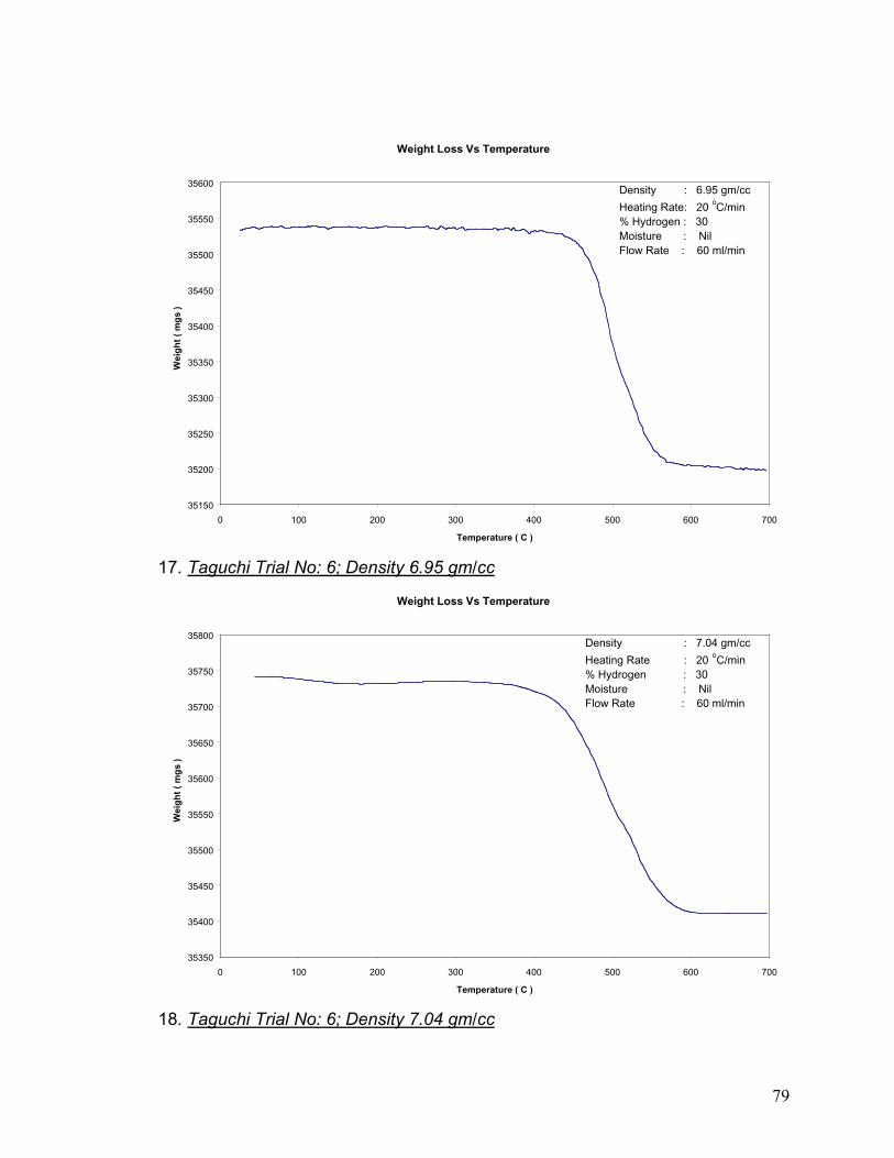
79
Weight Loss Vs Temperature
35150
35200
35250
35300
35350
35400
35450
35500
35550
35600
0 100 200 300 400 500 600 700
Temperature ( C )
Wei
gh
t (
mg
s )
Density : 6.95 gm/cc
Heating Rate: 20 oC/min% Hydrogen : 30Moisture : NilFlow Rate : 60 ml/min
17. Taguchi Trial No: 6; Density 6.95 gm/cc
Weight Loss Vs Temperature
35350
35400
35450
35500
35550
35600
35650
35700
35750
35800
0 100 200 300 400 500 600 700
Temperature ( C )
Wei
gh
t (
mg
s )
Density : 7.04 gm/cc
Heating Rate : 20 oC/min% Hydrogen : 30Moisture : NilFlow Rate : 60 ml/min
18. Taguchi Trial No: 6; Density 7.04 gm/cc

80
Weight Loss Vs Temperature
35050
35100
35150
35200
35250
35300
35350
35400
35450
0 100 200 300 400 500 600 700
Temperature ( C )
Wei
gh
t (
mg
s )
Density : 6.95 gm/cc
Heating Rate: 30 oC/min% Hydrogen : 5Moisture : HighFlow Rate : 60 ml/min
19. Taguchi Trial No: 7; Density 6.80 gm/cc

81
Weight Loss Vs Temperature
34400
34450
34500
34550
34600
34650
34700
34750
34800
0 100 200 300 400 500 600 700
Temperature ( C )
Wei
gh
t (
mg
s )
Density : 6.80 gm/cc
Heating Rate: 30 oC/min% Hydrogen : 5Moisture : HighFlow Rate : 60 ml/min
20. Taguchi Trial No: 7; Density 6.95 gm/cc

82
Weight Loss Vs Temperature
35100
35150
35200
35250
35300
35350
35400
35450
35500
35550
0 100 200 300 400 500 600 700
Temperature ( C )
Wei
gh
t (
mg
s )
Density : 7.04 gm/cc
Heating Rate : 30 oC/min% Hydrogen : 5Moisture : HighFlow Rate : 60 ml/min
21. Taguchi Trial No: 7; Density 7.04 gm/ccWeight Loss Vs Temperature
34600
34650
34700
34750
34800
34850
34900
34950
35000
0 100 200 300 400 500 600 700
Temperature ( C )
Wei
gh
t (
mg
s )
Density : 6.80 gm/cc
Heating Rate: 30 oC/min% Hydrogen : 15Moisture : NilFlow Rate : 80 ml/min
22. Taguchi Trial No: 8; Density 6.80 gm/cc

83
Weight Loss Vs Temperature
34400
34450
34500
34550
34600
34650
34700
34750
34800
0 100 200 300 400 500 600 700
Temperature ( C )
Wei
gh
t (
mg
s )
Density : 6.95 gm/cc
Heating Rate : 30 oC/min% Hydrogen : 15Moisture : NilFlow Rate : 80 ml/min
23. Taguchi Trial No: 8; Density 6.95 gm/cc
Weight Loss Vs Temperature
35050
35100
35150
35200
35250
35300
35350
35400
35450
0 100 200 300 400 500 600 700
Temperature ( C )
Wei
gh
t (
mg
s )
Density : 7.04 gm/cc
Heating Rate : 30 oC/min% Hydrogen : 15Moisture : NilFlow Rate : 80 ml/min
24. Taguchi Trial No: 8; Density 7.04 gm/cc

84
Weight Loss Vs Temperature
34200
34250
34300
34350
34400
34450
34500
34550
34600
0 100 200 300 400 500 600 700
Temperature ( C )
Wei
gh
t (
mg
s )
Density : 6.80 gm/cc
Heating Rate : 30 oC/min% Hydrogen : 30Moisture : LowFlow Rate : 40 ml/min
25.Taghuchi trial No 9; Density 6.95 gm/cc
Weight Loss Vs Temperature
34300
34350
34400
34450
34500
34550
34600
34650
34700
34750
34800
0 100 200 300 400 500 600
Temperature ( C )
Wei
gh
t (
mg
s )
Density : 6.95 gm/cc
Heating Rate : 30 oC/min% Hydrogen : 30Moisture : LowFlow Rate : 40 ml/min
26. Taguchi Trial No:9; Density 6.95 gm/cc

85
Weight Loss Vs Temperature
35400
35450
35500
35550
35600
35650
35700
35750
35800
35850
0 100 200 300 400 500 600 700
Temperature ( C )
Wei
gh
t (
mg
s )
Density : 7.04 gm/cc
Heating Rate : 30 oC/min% Hydrogen : 30Moisture : LowFlow Rate : 40 ml/min
27. Taguchi Trial No: 9; Density 7.04 gm/cc

86
APPENDIX C: WORKING PRINCIPLE OF FTIR
FTIR or Fourier Transform Infrared Spectroscopy is an instrument used to obtain
an infrared spectrum when infrared light passed through a sample. Most
dispersive instruments use a monochromator to split light into a spectrum of its
component wave number. A slit is used to select a narrow slice of wave numbers
before it strikes the detector.
IR source
Sample
Mirror
Grating
Detector
Figure 59: Schematic of a dispersive grating infrared spectrometer
In FTIR all of the infrared radiation passes and through the sample. There are on
restrictions on the wave number range that strikes the sample. The complete
range of wave numbers used provides a multiplex (or Fellgett) advantage. It is
based on fact that in an FTIR, all the wave numbers of the light are detected at
once, whereas in a dispersive instrument only a small wave number range at a

87
time is measured. Thus, acquiring data for 10 minutes on an FTIR means all
wave numbers are observed for a full 10 minutes. In a dispersive spectrometer
each wave number is observed for only a short fraction of the 10-minute
measurement time. A schematic of a non-dispersive interferometer is shown in
Figure 60.
Source
Moving Mirror
Fixed Mirror
Sample
Detector
Radiation
Beam splitter
Figure 60: Schematic of a Michelson interferometer
The heart of most FTIRs in use today, based on the principles of Michelsons
interferometer. Light from the source, is split by the beam —splitter. One half of
the beam is transmitted to a fixed mirror and the other strikes a moving mirror.
After reflection for the respective mirrors, the two beams recombine at the beam
splitter, to interact with the sample. If the moving mirror and the fixed mirror are
at the same distance from the beam splitter, the distance traveled by the light are

88
the same. This condition is called as zero path difference (ZPD). The
displacement of the moving mirror from the ZPD (called mirror displacement (∆)),
leads to the light traveling an extra distance. This distance is called the optical
path difference (δ). The relationship between mirror displacement and optical
path difference is shown in equation 1.
δ = 2∆ (1)
The presence of mirror displacement leads to the interference of light.
Constructive interference takes place when the optical path difference is an
integer multiple of λ. Destructive interference occurs when the optical path
difference is λ2
1 or some multiple of it.
Constructive Interference: δ = nλ (2)
Destructive Interference: δ = (n + 2
1)λ (3)
Where, n = 0,1,2,3,4,5,6, .
Interference leads to a light intensity is bright (constructive) and very weak
(destructive), depending on the optical path difference. If the mirror is moved at a
constant speed, the intensity of light increases and decreases smoothly. The
variation in light intensity is measured by the detector as a sinusoidal wave. A
plot of the light intensity versus optical path difference is called a interferogram.
Figure 61 shows a typical interferogram obtained from a FTIR. An interferogram

89
Figure 61: Interferogram and the fourier transform
Fourier Transform

90
is essentially a large number of sinusoidal waves added together. According to
Fouriers theorm, any mathematical function (an x,y plot) can be expressed as a
sum of sinusoidal waves. Fourier transform calculate the infrared spectrum and
form the interferogram. Fourier tranfroms have their X units transformed. Thus,
Fourier transform inverts the interfrogram to produces an infrared spectrum.

91
APPENDIX D: SPECTRUMS OF EXPERIMENT A AND B(Wave number in the X — axis Vs Absorbance in Y — axis)
Experiment A:
Background - A
0.00E+00
5.00E+00
1.00E+01
1.50E+01
2.00E+01
2.50E+01
3.00E+01
3.50E+01
0.00E+00 1.00E+03 2.00E+03 3.00E+03 4.00E+03 5.00E+03 6.00E+03 7.00E+03
Spectra A-1
-5.00E-01
0.00E+00
5.00E-01
1.00E+00
1.50E+00
2.00E+00
2.50E+00
3.00E+00
0.00E+00 1.00E+03 2.00E+03 3.00E+03 4.00E+03 5.00E+03 6.00E+03 7.00E+03

92
Spectra A-3
-5.00E-01
0.00E+00
5.00E-01
1.00E+00
1.50E+00
2.00E+00
2.50E+00
3.00E+00
0.00E+00 1.00E+03 2.00E+03 3.00E+03 4.00E+03 5.00E+03 6.00E+03 7.00E+03
Spectra A-2
-5.00E-01
0.00E+00
5.00E-01
1.00E+00
1.50E+00
2.00E+00
2.50E+00
3.00E+00
0.00E+00 1.00E+03 2.00E+03 3.00E+03 4.00E+03 5.00E+03 6.00E+03 7.00E+03

93
Spectra A-4
-5.00E-01
0.00E+00
5.00E-01
1.00E+00
1.50E+00
2.00E+00
2.50E+00
3.00E+00
0.00E+00 1.00E+03 2.00E+03 3.00E+03 4.00E+03 5.00E+03 6.00E+03 7.00E+03
Spectra A-5
-5.00E-01
0.00E+00
5.00E-01
1.00E+00
1.50E+00
2.00E+00
2.50E+00
3.00E+00
0.00E+00 1.00E+03 2.00E+03 3.00E+03 4.00E+03 5.00E+03 6.00E+03 7.00E+03

94
Spectra A-6
-5.00E-01
0.00E+00
5.00E-01
1.00E+00
1.50E+00
2.00E+00
2.50E+00
3.00E+00
0.00E+00 1.00E+03 2.00E+03 3.00E+03 4.00E+03 5.00E+03 6.00E+03 7.00E+03
Spectra A-7
-5.00E-01
0.00E+00
5.00E-01
1.00E+00
1.50E+00
2.00E+00
2.50E+00
3.00E+00
0.00E+00 1.00E+03 2.00E+03 3.00E+03 4.00E+03 5.00E+03 6.00E+03 7.00E+03

95
Spectra A-8
-5.00E-01
0.00E+00
5.00E-01
1.00E+00
1.50E+00
2.00E+00
2.50E+00
3.00E+00
0.00E+00 1.00E+03 2.00E+03 3.00E+03 4.00E+03 5.00E+03 6.00E+03 7.00E+03
Spectra A-9
-5.00E-01
0.00E+00
5.00E-01
1.00E+00
1.50E+00
2.00E+00
2.50E+00
3.00E+00
0.00E+00 1.00E+03 2.00E+03 3.00E+03 4.00E+03 5.00E+03 6.00E+03 7.00E+03

96
Spectra A-10
-5.00E-01
0.00E+00
5.00E-01
1.00E+00
1.50E+00
2.00E+00
2.50E+00
3.00E+00
0.00E+00 1.00E+03 2.00E+03 3.00E+03 4.00E+03 5.00E+03 6.00E+03 7.00E+03
Spetra A-11
-5.00E-01
0.00E+00
5.00E-01
1.00E+00
1.50E+00
2.00E+00
2.50E+00
3.00E+00
0.00E+00 1.00E+03 2.00E+03 3.00E+03 4.00E+03 5.00E+03 6.00E+03 7.00E+03

97
Spectra A-12
-5.00E-01
0.00E+00
5.00E-01
1.00E+00
1.50E+00
2.00E+00
2.50E+00
3.00E+00
0.00E+00 1.00E+03 2.00E+03 3.00E+03 4.00E+03 5.00E+03 6.00E+03 7.00E+03
Spectra A-13
-5.00E-01
0.00E+00
5.00E-01
1.00E+00
1.50E+00
2.00E+00
2.50E+00
3.00E+00
0.00E+00 1.00E+03 2.00E+03 3.00E+03 4.00E+03 5.00E+03 6.00E+03 7.00E+03

98
Spectra A-14
-5.00E-01
0.00E+00
5.00E-01
1.00E+00
1.50E+00
2.00E+00
2.50E+00
3.00E+00
0.00E+00 1.00E+03 2.00E+03 3.00E+03 4.00E+03 5.00E+03 6.00E+03 7.00E+03
Spectra A-15
-5.00E-01
0.00E+00
5.00E-01
1.00E+00
1.50E+00
2.00E+00
2.50E+00
3.00E+00
0.00E+00 1.00E+03 2.00E+03 3.00E+03 4.00E+03 5.00E+03 6.00E+03 7.00E+03

99
Spectra A-16
-5.00E-01
0.00E+00
5.00E-01
1.00E+00
1.50E+00
2.00E+00
2.50E+00
3.00E+00
0.00E+00 1.00E+03 2.00E+03 3.00E+03 4.00E+03 5.00E+03 6.00E+03 7.00E+03
Spectra A-17
-5.00E-01
0.00E+00
5.00E-01
1.00E+00
1.50E+00
2.00E+00
2.50E+00
3.00E+00
0.00E+00 1.00E+03 2.00E+03 3.00E+03 4.00E+03 5.00E+03 6.00E+03 7.00E+03

100
Spectra A-18
-5.00E-01
0.00E+00
5.00E-01
1.00E+00
1.50E+00
2.00E+00
2.50E+00
3.00E+00
0.00E+00 1.00E+03 2.00E+03 3.00E+03 4.00E+03 5.00E+03 6.00E+03 7.00E+03
Spectra A-19
-5.00E-01
0.00E+00
5.00E-01
1.00E+00
1.50E+00
2.00E+00
2.50E+00
3.00E+00
0.00E+00 1.00E+03 2.00E+03 3.00E+03 4.00E+03 5.00E+03 6.00E+03 7.00E+03

101
Experiment B:
Background - B
0.00E+00
5.00E+00
1.00E+01
1.50E+01
2.00E+01
2.50E+01
3.00E+01
3.50E+01
0.00E+00 1.00E+03 2.00E+03 3.00E+03 4.00E+03 5.00E+03 6.00E+03 7.00E+03
Specta B-1
-7.00E-02
-6.00E-02
-5.00E-02
-4.00E-02
-3.00E-02
-2.00E-02
-1.00E-02
0.00E+00
1.00E-02
2.00E-02
0.00E+00 1.00E+03 2.00E+03 3.00E+03 4.00E+03 5.00E+03 6.00E+03 7.00E+03

102
Spectra B-4
-5.00E-03
0.00E+00
5.00E-03
1.00E-02
1.50E-02
2.00E-02
2.50E-02
3.00E-02
3.50E-02
4.00E-02
0.00E+00 1.00E+03 2.00E+03 3.00E+03 4.00E+03 5.00E+03 6.00E+03 7.00E+03
Spectra B-3
-1.00E-01
-8.00E-02
-6.00E-02
-4.00E-02
-2.00E-02
0.00E+00
2.00E-02
0.00E+00 1.00E+03 2.00E+03 3.00E+03 4.00E+03 5.00E+03 6.00E+03 7.00E+03

103
Spectra B-5
-1.00E-02
0.00E+00
1.00E-02
2.00E-02
3.00E-02
4.00E-02
5.00E-02
6.00E-02
7.00E-02
8.00E-02
9.00E-02
1.00E-01
0.00E+00 1.00E+03 2.00E+03 3.00E+03 4.00E+03 5.00E+03 6.00E+03 7.00E+03
Spectra B-6
-1.00E-02
0.00E+00
1.00E-02
2.00E-02
3.00E-02
4.00E-02
5.00E-02
6.00E-02
7.00E-02
0.00E+00 1.00E+03 2.00E+03 3.00E+03 4.00E+03 5.00E+03 6.00E+03 7.00E+03

104
Spectra B-7
-1.50E-02
-1.00E-02
-5.00E-03
0.00E+00
5.00E-03
1.00E-02
1.50E-02
2.00E-02
0.00E+00 1.00E+03 2.00E+03 3.00E+03 4.00E+03 5.00E+03 6.00E+03 7.00E+03
Spectra B-8
-4.00E-02
-3.00E-02
-2.00E-02
-1.00E-02
0.00E+00
1.00E-02
2.00E-02
3.00E-02
0.00E+00 1.00E+03 2.00E+03 3.00E+03 4.00E+03 5.00E+03 6.00E+03 7.00E+03

105
Spectra B-9
-2.00E-02
-1.00E-02
0.00E+00
1.00E-02
2.00E-02
3.00E-02
4.00E-02
5.00E-02
6.00E-02
0.00E+00 1.00E+03 2.00E+03 3.00E+03 4.00E+03 5.00E+03 6.00E+03 7.00E+03
Spectra B-10
-4.00E-02
-2.00E-02
0.00E+00
2.00E-02
4.00E-02
6.00E-02
8.00E-02
1.00E-01
1.20E-01
1.40E-01
0.00E+00 1.00E+03 2.00E+03 3.00E+03 4.00E+03 5.00E+03 6.00E+03 7.00E+03

106
Spectra B-11
-5.00E-02
0.00E+00
5.00E-02
1.00E-01
1.50E-01
2.00E-01
2.50E-01
3.00E-01
3.50E-01
4.00E-01
4.50E-01
0.00E+00 1.00E+03 2.00E+03 3.00E+03 4.00E+03 5.00E+03 6.00E+03 7.00E+03
Spectra B-12
-1.00E-01
0.00E+00
1.00E-01
2.00E-01
3.00E-01
4.00E-01
5.00E-01
6.00E-01
7.00E-01
8.00E-01
0.00E+00 1.00E+03 2.00E+03 3.00E+03 4.00E+03 5.00E+03 6.00E+03 7.00E+03

107
Spectra B-13
-1.00E-01
0.00E+00
1.00E-01
2.00E-01
3.00E-01
4.00E-01
5.00E-01
6.00E-01
7.00E-01
8.00E-01
0.00E+00 1.00E+03 2.00E+03 3.00E+03 4.00E+03 5.00E+03 6.00E+03 7.00E+03
Spectra B-14
-2.00E-01
0.00E+00
2.00E-01
4.00E-01
6.00E-01
8.00E-01
1.00E+00
1.20E+00
1.40E+00
1.60E+00
0.00E+00 1.00E+03 2.00E+03 3.00E+03 4.00E+03 5.00E+03 6.00E+03 7.00E+03

108
Spectra B-15
-2.00E-01
0.00E+00
2.00E-01
4.00E-01
6.00E-01
8.00E-01
1.00E+00
1.20E+00
1.40E+00
0.00E+00 1.00E+03 2.00E+03 3.00E+03 4.00E+03 5.00E+03 6.00E+03 7.00E+03
Spectra B-16
-1.00E-01
0.00E+00
1.00E-01
2.00E-01
3.00E-01
4.00E-01
5.00E-01
6.00E-01
7.00E-01
0.00E+00 1.00E+03 2.00E+03 3.00E+03 4.00E+03 5.00E+03 6.00E+03 7.00E+03

109
Spectra B-17
-5.00E-02
0.00E+00
5.00E-02
1.00E-01
1.50E-01
2.00E-01
2.50E-01
3.00E-01
3.50E-01
4.00E-01
4.50E-01
0.00E+00 1.00E+03 2.00E+03 3.00E+03 4.00E+03 5.00E+03 6.00E+03 7.00E+03
Spectra B-18
-5.00E-02
0.00E+00
5.00E-02
1.00E-01
1.50E-01
2.00E-01
2.50E-01
3.00E-01
3.50E-01
0.00E+00 1.00E+03 2.00E+03 3.00E+03 4.00E+03 5.00E+03 6.00E+03 7.00E+03

110
Spectra B-19
-5.00E-02
0.00E+00
5.00E-02
1.00E-01
1.50E-01
2.00E-01
2.50E-01
3.00E-01
0.00E+00 1.00E+03 2.00E+03 3.00E+03 4.00E+03 5.00E+03 6.00E+03 7.00E+03

111
APPENDIX E: ACTUAL AND PREDICTED DATA OF THE MODEL
Actual Vs Predicted Weight Vs Time for Green Density 6.80 gm/cc (Trial 1)
0
50
100
150
200
250
300
350
400
0 500 1000 1500 2000 2500 3000 3500 4000 4500
Time (secs)
Wei
ght (
mgs
)
1680
1680Pr
Heating Rate = 10 0C/mint(max) = 2647b = 20.39
Actual Vs Predicted weight Vs Time for Green Density 6.95 gm/cc (Trial 1)
0
50
100
150
200
250
300
350
400
0 500 1000 1500 2000 2500 3000 3500 4000
Time (secs)
Wei
ght (
mgs
) 1695
1695Pr
Heating Rate = 10 0C/mint(max) = 2652b = 20.42

112
Actual Vs Predicted weights Vs Time for Green Density 6.80 gm/cc (Trial 2)
0
50
100
150
200
250
300
350
0 500 1000 1500 2000 2500 3000 3500 4000 4500
Time (Secs)
Wei
ght (
gms) 2680
2680Pr
Heating Rate = 10 0C/mint(max) = 2678b = 23.64
Actual and Predicted Weight Vs Time for green Density 6.95 gm/cc (Trial 2)
0
50
100
150
200
250
300
350
0 500 1000 1500 2000 2500 3000 3500 4000 4500
2695
2695Pr
Heating Rate = 10 0C/mint(max) = 2593b = 22.44

113
Actual and predicted weights Vs Time for Green Density 7.04 (Trial 2)
0
50
100
150
200
250
300
350
400
0 500 1000 1500 2000 2500 3000 3500 4000 4500
Time (secs)
Wei
ght (
mgs
)
2704
2704Pr
Heating Rate = 10 0C/mint(max) = 2705b = 23.44
Actual and Predicted weights Vs Time for Green Density 6.80 gm/cc (Trial 3)
0
50
100
150
200
250
300
350
400
0 500 1000 1500 2000 2500 3000 3500 4000 4500
Time (secs)
Wei
ght (
mgs
)
3680
3680Pr
Heating Rate = 10 0C/mint(max) = 2651b = 22.57

114
Actual Vs Predicted weight Vs Time for Green Denisty 6.95 gm/cc (Trial 3)
0
50
100
150
200
250
300
350
400
0 500 1000 1500 2000 2500 3000 3500 4000 4500
Time (secs)
Wei
ght (
mgs
) 3695
3695Pr
Heating Rate = 10 0C/mint(max) = 2489b = 21.19
Actual Vs Predicted Weight for Green Denisty 7.04 gm/cc (Trial 3)
0
50
100
150
200
250
300
350
400
0 500 1000 1500 2000 2500 3000 3500 4000 4500
Time (secs)
Wei
gth
(mgs
) 3704
3704Pr
Heating Rate = 10 0C/mint(max) = 2684b = 23

115
Actual Vs Predicted ( Average of the ’b’ and ’c’ of the actual values)Heating Rate ---------- 10 0C/min
0
50
100
150
200
250
300
350
400
0 500 1000 1500 2000 2500 3000 3500 4000
Time (secs)
Wei
ght o
f the
Lub
rica
nt (m
gs)
16801695268026952704368036953704Average(Pr)
Heating Rate = 10 0C/mint(max) = 2637b = 22.15
Predicted Vs Actual ( Average of ’c’ and ’b’ of the actual values )Heating Rate -------- 30 0C/min
0
50
100
150
200
250
300
350
400
0 200 400 600 800 1000 1200 1400
Time(secs)
Wei
ght o
f the
Lub
rica
nt (m
gs) 7680
868096807695
86959695770487049704Average

116
ATTACHMENT II
RECOMMANDATIONS FOR FUTURE WORK

117
This section deals with the various suggestions and recommendations resulting
from this work.
• Phase 2 of our study clearly shows that the breakdown of EBS results in the
release of gases such as CO2, CO, NH3 and heptadecane which can be
detected using a sensor. Development of sensors, which would detect the
concentration of CO2 and heptadecane is a real possibility. The
concentrations of CO and NH3 are however, too low (< 60 ppm) to be
economically viable. The sensor would need a non-dispersive IR absorption
spectroscopy as its modus operandi.
• As heptadecane has a sublimation of 1400C, the problem of sooting can be
related to the condensation of this high molecular weight hydrocarbon in the
cooler parts of the furnace (front) onto the parts. As the part gets heated in
the de-lubrication zone, the hydrocarbon decomposes by thermal pyrolysis
to carbon or soot on the furnace. Preheating the parts or increasing the
furnace temperature in the front zone of the furnace to above the
sublimation of heptadecane might solve the problem of sooting . This might
explain the increased incidence of sooting during the sintering of high Ni
parts. It is well known that Ni is a very good catalyst (commonly used in the
hydrogenation of oils), presence of hydrogen, a heavy weight hydrocarbon
and Ni can lead to the rapid breakdown of the lubricant / heptadecane to
free carbon. This hypothesis however, needs to investigated and studied in
detail.
• Phase III of our research clearly shows that the mathematical model can be
used an algorithm in the control system . The values of b reported in phase
II, are values determined for a Fe — 0.8 C compacted system. In reality, b

118
incorporates into it, the thermal properties of the alloy used. For the model
to be applicable to industrial furnaces, the database of b for various alloy
system should be determined. This would make the control system Alloy
independent .

119
ATTACHMENT III

120
Objective:
To identify the primary fracture mechanism in sintering furnace belts
Analysis of fractured sintering belt samples:
Abbot Furnaces provided the fractured belt samples. The composition of theparent material is listed in Table I.Alloy Cr Ni Fe C Si Mn314 23 -26 19 - 22 BAL 0.25 (max) 1.5 (max) 2.0 (max)
Fracture analysis was performed in two parts- The fractured surface was observed for to understand the fracture
mechanism
- The samples were then cut and observed to see the microstructure details
Result:
Figure 1 — 3 show the defective part of the belt. The fractured strands werecollected and observed under the SEM for analysis. The topographic results(Figure 4) clearly show that the primary mechanism for failure is graincoarsening. Analysis of the fractured surface showed the presence ofprecipitates on the surface. The precipitates are shown in Figure 5. The size (5 —20 µm) and distribution of the precipitates show that there was a growth inprecipitates due to high heat. Figure 6 shows the precipitates at highermagnification. An important observation is the faceted structure of the precipitate.Figure 7 shows the presence of holes in the precipitate. The holes wereobserved in 60 —70 % of the precipitates. This suggests the presence of highvapor pressure element in the precipitate. As the steel is rich in Chromium,presences of these holes suggest a chromium rich precipitate (the vaporpressure of chromium is high). The precipitate was identified as shown in Figure9 —10. Figure 9 is a line analysis across the grain boundary. The composition ofprecipitate clearly shows an increased amount of Chromium and a drop in theconcentration of Ni and Fe. Figure 10 is a X-Map across the gain boundary. Itclearly shows the presence of chromium rich precipitates (light regions show therich phase element) along the grain boundary.
Recommendations:
The primary mechanism for the belt failure is due to grain boundary weakening.Following are the recommendations for improvement in belt life:
• Chromium carbides are normally in the form of M23C6. These lead to adeletion of chromium along the grain boundary and hence, corrosionprone. Increasing the addition of stable carbide formers, like Titanium orVanadium prevents the formation of these carbides as these elements

121
• readily react with free carbon to form stable carbides, reducing theincidence of corrosion.
• Switching to high Ni steels, as the solubility of carbon is less in Nickel richsteels.
• Preventing the diffusion of Carbon during de-lubrication by diffusionbarriers. Though Aluminum coating has shown promise, there exists avery good potential to develop coatings to prevent carbon diffusion.
Analysis:
Fractured belts were supplied by Abbot furnace. The pictures of the belt strandsare shown in Figure 1 — 3
Fractured
belt strands
Figure 1: Fractures belt samples

122
Close up showing the
weakened strands
Figure 2: Close up of Figure 1
Figure 3: Fractured strands in a sintering belt

123
Figure 4: Topographic image of the fractured strand (30 X).
Fracture by grain coarsening
Figure 5: SEM image showing the presence of precipitates on
grain the boundary (2000X)

124
Figure 6: Precipitate (3000X)
Figure 7: Precipitate (6000X)

125
Figure 8: Grain boundary weakening by precipitation (60X),
etched by Carapella s reagent
Figure 9: Identification of precipitate by line scan (Chromium rich
precipitate)

126
Image Chromium Iron
Figure 10: X-Map along the grain boundary (light regions rich in the
element mapped).
INTERESTING FEATURES OBSERVED:
Figure 11: Christmas tree around the fractured surface (polished)

127
Image Copper
Chromium Iron
Figure 12: X-Map of the Christmas tree (Copper rich phase)