· pdf fileuniversite de nice sophia antipolis´ memoire´ present´ e pour...
TRANSCRIPT

UNIVERSITE DE NICE SOPHIA ANTIPOLIS
Memoire
presente pour obtenir le diplome d’
Habilitation a Diriger des Recherches
en Sciences Fondamentales et Appliquees
Specialite: Mathematiques
par
Martine OLIVI
Parametrization of rational lossless matriceswith applications to linear systems theory
soutenue le 25 Octobre 2010 devant le jury compose de
Laurent BARATCHART INRIA Sophia-Antipolis DirecteurBernhard BECKERMANN Universite de Lille RapporteurHugue GARNIER Universite de Nancy (CRAN) ExaminateurTryphon GEORGIOU University of Minnesota RapporteurJan MACIEJOWSKI University of Cambridge ExaminateurPaul VAN DOOREN Universite Catholique de Louvain Rapporteur


Contents
Introduction 1
1 Lossless functions in system theory 5
1.1 Transfer functions and their factorizations . . . . . . . . . . . . . . . . . . 6
1.1.1 The algebraic framework . . . . . . . . . . . . . . . . . . . . . . . 6
1.1.2 The geometric framework . . . . . . . . . . . . . . . . . . . . . . . 9
1.1.3 Inner matrix-valued functions . . . . . . . . . . . . . . . . . . . . 12
1.2 Realization theory and balanced canonical forms . . . . . . . . . . . . . . 12
1.2.1 Realization theory . . . . . . . . . . . . . . . . . . . . . . . . . . . 13
1.2.2 Null-pole triples and pole-zero structure . . . . . . . . . . . . . . 16
1.2.3 Balanced realizations and canonical forms . . . . . . . . . . . . . 17
1.3 Interpolation and parametrization . . . . . . . . . . . . . . . . . . . . . . 18
1.3.1 J-inner functions and linear fractional transformations. . . . . . . 19
1.3.2 J-lossless and lossless embedding . . . . . . . . . . . . . . . . . . 21
1.3.3 The Nudelman interpolation problem. . . . . . . . . . . . . . . . . 22
1.3.4 The tangential Schur algorithm vs Potapov factorization . . . . . 23
1.3.5 Parametrizations from the tangential Schur algorithm. . . . . . . 25
2 Schur vectors and balanced canonical forms for lossless systems 29
2.1 Balanced canonical forms from the tangential Schur algorithm. . . . . . . 30
2.2 Canonical forms with a pivot structure . . . . . . . . . . . . . . . . . . . . 34
2.2.1 Subdiagonal canonical forms from the Schur algorithm . . . . . . 34
2.2.2 Subdiagonal canonical forms under state isometry . . . . . . . . . 36
2.2.3 Staircase canonical forms . . . . . . . . . . . . . . . . . . . . . . . 37
2.3 Perspectives . . . . . . . . . . . . . . . . . . . . . . . . . . . . . . . . . . . 41
3 Rational H2 approximation and lossless mutual encoding 45

ii CONTENTS
3.1 The rational approximation problem . . . . . . . . . . . . . . . . . . . . . 46
3.2 Nudelman interpolation and lossless mutual encoding . . . . . . . . . . 47
3.3 RARL2 : a rational approximation software . . . . . . . . . . . . . . . . . 51
3.4 Identification of microwave filters. . . . . . . . . . . . . . . . . . . . . . . 55
3.5 More applications . . . . . . . . . . . . . . . . . . . . . . . . . . . . . . . . 56
3.5.1 Localization of dipolar sources in electroencephalography. . . . . 57
3.5.2 Multi-objective control. . . . . . . . . . . . . . . . . . . . . . . . . 59
3.5.3 Wavelets approximation . . . . . . . . . . . . . . . . . . . . . . . . 59
3.6 Perspectives. . . . . . . . . . . . . . . . . . . . . . . . . . . . . . . . . . . . 60
4 Symmetric lossless matrix-valued extensions of rational contractions 63
4.1 The scalar case . . . . . . . . . . . . . . . . . . . . . . . . . . . . . . . . . . 64
4.2 From Darlington synthesis to symmetric extensions . . . . . . . . . . . . 65
4.3 Minimal degree vs minimal size symmetric extensions . . . . . . . . . . 68
4.4 Perspectives . . . . . . . . . . . . . . . . . . . . . . . . . . . . . . . . . . . 71

Introduction
The works presented in this habilitation thesis were initially motivated by the rationalapproximation issue in system theory.Rational matrix-valued functions arise with the transfer function description of a fi-nite dimensional, linear, time-invariant system. Rational approximation seems to methe main issue in the fundamental modelization problem: given some data about asystem, find the best model in the popular class of LTI systems. This problem canbe understood in many different ways and resulted in many approaches dependingon the nature of the data (time series, frequency data), on the purpose of the model(prediction, control), etc. . The current approaches mainly fall in two sub-classes, theprojection methods (subspace method, balanced truncation) easy to implement butnot always efficient, and optimization methods (Hankel, H2) which result in difficultnon-linear problems. Model reduction and identification are still very active fields insystem theory as numerous recent publications show [3, 24, 58].
Our contribution was dedicated to rational approximation in the Hardy space H2.This space is interesting both for its underlying stochastic interpretation and the Hilber-tian framework it provides. It corresponds for the transfer function to a L2 7→ L∞ sta-bility requirement (a finite energy input produces a bounded energy output). Givena transfer function in H2, the rational approximation problem is thus to minimize thedistance in L2-norm to the set of rational stable transfer functions of order at most n.This problem features some serious difficulties : it is a non-linear optimization prob-lem, the set of approximants has a complicated structure and the L2-error may possessa great number of local minima in which a descent algorithm can get stuck. To copewith these problems, we have developed an original approach [BCO91, FO98] basedon
• a compactification of the optimization set which makes use of the Douglas-Shapi-ro-Shields factorization and the projection theorem in Hilbert space. Losslessmatrix valued functions play in the matrix case the role of the denominator inthe scalar case. The ”denominator” is thus optimized while the ”numerator” iscomputed by projection: the optimization runs over the set of lossless functionswhich thus enter the picture and bring their rich structure. Surprisingly enough,this method is seldom used in approximation; it is known, in the context of least-square approximation, under the name ”separable least-squares”.
• the use of an atlas of charts to describe the optimization set: the space of losslessfunctions of fixed McMillan degree. This type of representation is recommendedif one wants to use differential calculus tools for solving an optimization prob-

2 Introduction
lem. The first atlas of charts for lossless matrix valued functions were obtainedin [1] from a tangential Schur algorithm. An important part of this document isdevoted to the description of such atlases.
Rational approximation was our first motivation to study lossless functions and theirparametrizations. However, these functions play an important role in system theoryanyway because of the Douglas-Shapiro-Shields factorization. They also are of inde-pendent interest, being the transfer functions of conservative systems: the scatteringmatrix of a frequency filter, the polyphase matrix of an orthogonal filter bank are loss-less. Overall, they lie at the heart of Schur analysis, a rich theory studying interpolationproblems for functions satisfying a metric constraint, namely Schur functions (see e.g.[18, 4, 20]). This gives rise to multiple interactions with system theory [35, 40] and haswidely inspired this work.
Concerning the parametrization of lossless (matrix-valued) functions, we aimed atconnecting two types of representations
• atlases of charts derived from interpolation problems. The parameters are thusinterpolation values. This is a very efficient way to take into account the Schurmetric constraint and subsequently the stability requirement.
• state-space representations and balanced canonical forms. State-space represen-tations involve basically linear algebra techniques and their efficiency for numer-ical computations has been demonstrated.
In [31], such a connection was established between the Hessenberg canonical form fordiscrete-time scalar systems and the Schur algorithm. The Hessenberg canonical formis balanced and such that, in addition, the associated controlability matrix is upper-triangular. The state-space realization can be written as a product of Givens rotationswhose parameters are precisely the sequence Schur parameters. In chapter 2, the re-sults of [31] are generalized to the matrix case following the approach developed in[HOP06, PHO07, HOP09]. Overlapping balanced canonical forms are associated witha suitable tangential Schur algorithm. Realization matrices are obtained as a product ofunitary matrices that can be parametrized by a sequence of vectorial Schur parameters.Moreover, for a canonical choice of interpolation values and interpolation directions inthe Schur algorithm, the realization matrix possesses a sub-diagonal pivot structure.It generalizes the Hessenberg form of the SISO (single input-single output) case andshould be a useful tool for model reduction.
Chapter 3 is dedicated to H2 rational approximation and its practical implemen-tation in the software RARL2. Another atlas of charts is used here, which has beenconstructed from more general interpolation data [MO07]. In this atlas, a chart is in-dexed by a lossless transfer function whose parameters are all zero, which explains thedenomination ”lossless mutual encoding” for this parametrization. It exhibits severalnice features, in particular computational simplicity and the fact that it better suits therepresentation of real or conjugate symmetric lossless functions. This is an importantpoint, since real-world systems and their transfer functions are usually real. The soft-ware RARL2 [MO04] is mainly used for two dedicated applications, for which it iscombined with other tools into specific softwares: PRESTO-HF for the identificationof microwave filters from frequency data [60] and FINDSOURCE3D for the localiza-

3
tion of dipolar sources in electroencephalography [8]. Potential applications abound,among which wavelet approximation and aircraft flutter modal parameter identifica-tion are already under investigation.
More recently, motivated by microwave filter design applications, we worked on acompletion problem for matrix valued lossless systems. Frequency filters are usuallydescribed by scattering matrices which are not only lossless but also symmetric, dueto the reciprocity law attached to wave propagation. Since the design problem bearson a submatrix (the transmission), it would be interesting to characterize the subma-trices of a lossless symmmetric matrix. This problem can be stated as follows: underwhich conditions can a symmetric Schur matrix be extended into a lossless one? Werecast the celebrated Darlington synthesis problem [15] with an additional symme-try requirement which refines the completion problem. In Chapter 4 we summarizethe contribution of [BEGO07] which significantly improves previous results [2] andprovides both a minimal degree extension of double dimension and a minimal dimen-sion extension of the same degree. These results brings a new understanding of thestructure of 3× 3 reciprocal matrices and the derivation of efficient algorithm for thesynthesis of 3-ports devices is being studied.

4 Introduction

Chapter 1
Lossless functions in system theory
Lossless systems and their transfer functions are involved in many areas of systemtheory, from electrical network theory and related synthesis problems [2] to moderndigital signal processing [63]. A lossless system is a device which conserves energy,as electrical networks with no resistive elements. The usefulness of lossless transferfunctions is also and mainly due to the Douglas-Shapiro-Shields factorization. Theyindeed appear as generalized denominators of rational matrix-valued functions.
In an engineering context, linear systems have been studied since the 1930s. An in-put/output and frequency domain viewpoint prevailed and SISO systems were mod-eled by their transfer functions. In the sixties, the move to state space models openthe way to new mathematical fields. The input/state/output systems had much moremodeling power, were far richer mathematically and took into consideration initialconditions, something that transfer functions fail to do. Mathematical system theorywas rapidly growing. The algebraic setting and the concept of module turned out tobe essential to deal with multivariable or MIMO (multi-input, multi-output) systems[37, 36]. The works of Fuhrmann, that we mainly follow, aimed at synthesizing thealgebraic approach of Kalman, the state-space approach as well as the polynomial ap-proach of Rosenbrock [56]. Functional analysis methods and geometry, relying on astability assumption, happened to be relevant in many purposes and nowadays clas-sical [23]. From a mathematical viewpoint, lossless functions arise with this geometricframework, namely associated with the invariant subspaces of the Hardy space H2.The reader interested by the history of mathematical systems theory should have alook at Willems’s essay [64].
In this chapter, we go over the now classical representations of finite-dimensionalLTI systems from transfer functions to state-space descriptions [23], and then glideto interpolation theory for rational systems as developed in [4]. The state and thepole-zero structure of the transfer function are the key concepts and lossless functionsthe heroes of this chapter. We focus on discrete-time systems that is, from a complexanalysis viewpoint, to the framework of the unit disk which is in some sense sim-pler. Our studies mostly bear on discrete-time lossless matrices, except in Chapter 4.The discrete-time and continuous-time settings are connected through a bilinear (orMobius) transformation of the variable (see e.g. [27] and section 3.4).

6 Lossless functions in system theory
1.1 Transfer functions and their factorizations
From an input/output viewpoint, a discrete-time system is modeled by a map :
σ : (uk)k∈Z 7→ (yk)k∈Z, uk ∈ Fm, yk ∈ Fp, F = R or C.
Linearity together with time-invariance of the system induces a discrete convolutionoperator. Putting more structure on the input and output signals spaces, allows torephrase systems properties (causality, stability) in mathematical terms. The two ap-proaches described in this section follow two parallel lines, splitting the time axis intwo parts, modeling the state and translating shift-invariance into commutation prop-erties.
1.1.1 The algebraic framework
Assuming the system initially at rest, algebra enters the picture representing input andoutput by truncated Laurent series and the system as a map
σ : F((1/z))m −→ F((1/z))p
u(z) = ∑ ukz−k 7→ y(z) = ∑ ykz−k .
The set of truncated Laurent series F((1/z)) is the quotient field of the set of formalseries F[[1/z]]. Linearity and time-invariance of the system imply that σ is a lineartransformation of vector spaces. The input/output behavior of the system is then com-pletely described by the multiplication by a matrix-valued function called the transferfunction of the system
y(z) = T(z)u(z).
Causality of the system implies that T(z) is proper, T(z) ∈ F[[1/z]]p×m.
With the concept of state, the module structure appears as the basic structure in thiscontext. The state is the memory of the system: at t = k, the state xk is the informationthat together with uk determines uniquely the output y(t) for all t > k. To address thisconcept, the time axis is divided in two parts, writing F((1/z)) as a direct sum
F((1/z) = F[z]⊕ 1/zF[1/z],
in which F[z] denotes the ring of polynomials over F. This decomposition is obtainedfrom the exact sequence of F[z]-modules:
0→ F[z]injection−−−−→ F((1/z))
projection−−−−−→ F((1/z))/F[z]︸ ︷︷ ︸1/zF[[1/z]]
−→ 0
The past-input to future-output map σ is then defined by the following commutativediagram
F((1/z))m σ−→ F((1/z))p
π+ ↓ ↓ π−
F[z]m σ−→ 1/zF[[1/z]]p

1.1 Transfer functions and their factorizations 7
The kernel of σ, ker σ, is a sub-module of the free module F[z]m over the PID (prin-cipal ideal domain) F[z].
ker σ = u(z) ∈ F[z]m; T(z)u(z) ∈ F[z]p . (1.1)
The structure of such sub-modules is well-known and described by the followingtheorem ([34, II, Ch. 3], [23]).
Theorem 1.1.1 (Adapted basis) Every sub-module E of a finitely generated free moduleM over a PID R, is free. There exists a basis (e1, e2, . . . , em) of M and a set of elementsd1, d2, ...ds, s ≤ m ofR such that di/di+1 and (d1e1, d2e2, . . . , dses) is a basis of E .
In our case, any basis of F[z]m consists in the columns of a unimodular matrix, a matrixwhich is invertible in F(z)m×m (its determinant is a constant). Theorem 1.1.1 assertsthat ker σ is spanned by the columns of a m × m polynomial matrix D(z), ker σ =D(z)F[z]m and D(z) is of the form
D(z) = U(z)diag(d1(z), d2(z), . . . , ds(z), 0, . . . , 0)V(z) (1.2)
• U(z) is a unimodular matrix,
• d1(z), d2(z), . . . , ds(z), are uniquely defined polynomials, with unit leading coef-ficients, satisfying the divisibility conditions di/di+1 for i = 1, . . . , s − 1, calledthe invariant factors,
• V(z) is a unimodular matrix that can be chosen arbitrarily.
Formula (1.2) is known as the Smith form of a polynomial matrix. The product d1...dkof the invariant factors is the g.c.d. of the k× k minors of D(z) [34, II, Chap. 3, Sec. 9].The Smith form also exists for a rectangular matrix.
Clearly, the state-space concept can be modeled by the quotient module
X = F[z]m/ker σ,
that is the set of equivalence classes for the relation induced by ker σ in F[z]m: f ∼ gif σ f = σg. We get the following commutative diagram, where π is a projection and ιan injection. The state-space can be viewed either as the quotient module X or as the
F[z]m σ−→ 1/z F[[1/z]]p
π ι
F[z]m/ ker σ︸ ︷︷ ︸X
Figure 1.1: The state space.
range of the injection ι and thus as a sub-module of 1/z F[[1/z]]p or else as a vectorspace over F. This triple nature is at the heart of realization theory (see section 1.2).
A LTI system is called finite order if X is a finite dimensional vector space over F.Finite-dimensional LTI systems are characterized by rational transfer functions whichis a consequence of

8 Lossless functions in system theory
Theorem 1.1.2 The following assertions are equivalent:
• ker σ is a full sub-module (m generators)
• D(z) is non-singular
• X is a torsion module. It is a direct sum of cyclic sub-modules: X =⊕ F[z]
diF[z] , the di’sbeing the invariant factors of D(z).
In this case, X is a finite dimensional vector space over F. The order of the system is defined asdimFX = ∑i deg di = deg(det D(z)).
From now on, we restrict ourselves to the study of finite dimensional LTI systems. Anumber of important representation results follow from the structure of ker σ, as thematrix fraction description [16] or the Smith-McMillan form [50].
The columns of D(z) belong to ker σ and thus T(z)D(z) must be a polynomial matrixN(z); D(z) being invertible, we get the matrix fraction description (MFD)
T(z) = N(z)D(z)−1 (1.3)
This factorization is called a right MFD, it has been obtained working with the columnsof the matrix, which is quite natural in this input/output context. However, workingwith the rows yields a dual representation, the left MFD, T(z) = D(z)−1N(z).
The Smith-McMillan form is a simple extension of the Smith form (1.2) in the rectan-gular case. It is obtained from T(z) = P(z)/q(z), where q(z) is a common denomina-tor of the rational entries of T(z) and P(z) a polynomial matrix, writing P(z) in Smithform.
Theorem 1.1.3 (Smith-McMillan form) Any rational function matrix T(z) can be writtenin the form
T(z) = U(z)diag n1(z)/d1(z), ..., nr(z)/dr(z), 0, ..., 0V(z) (1.4)
with
• U(z) and V(z) unimodular matrices
• ni and di are coprime polynomials, with unit leading coefficients, satisfying the divisibil-ity properties
n1|n2|...|nr and dr|dr−1|...|d1.
The matrix Λ(z) = n1(z)/d1(z), ..., nr(z)/dr(z), 0, ... is called the Smith-McMillan formof T(z) and is uniquely defined: it is canonic.
The non-negative integer r is the normal rank of T(z): there exists at least one minorof order r which does not vanish identically, and all minors of order greater than rvanish identically.
From a naive point of view, a pole of a rational matrix function is a pole of any ofits entry, but this definition neglects the problem of assigning multiplicities. The SmithMcMillan form is the simplest way to define poles and zeros for a rational matrixfunction:

1.1 Transfer functions and their factorizations 9
• the pole polynomial is defined as d(z) = d1(z)d2(z) . . . dr(z) and its roots are thepoles of the transfer matrix T(z).
• the zero polynomial is defined as n(z) = n1(z)n2(z) . . . nr(z) and its roots are thezeros or transmission zeros of the transfer matrix T(z).
A zero is a point where the local rank of N(z) in (1.3) drops below the normal rank[16]. It is important to notice that n(z) and d(z) are not necessarily relatively prime. Arational matrix can have a pole and a zero at the same location z = ω which do notcancel. The McMillan degree of a rational matrix is defined to be supdeg n, deg d. Inthe case of a proper (analytic at ∞) transfer function, the McMillan degree is the totalnumber of poles (with multiplicity). It is given by deg[d(z)] and coincides with theorder of the system.
The location and multiplicity of poles and zeros are essential to fully understand thecharacteristics of a multivariable system. If we write, for some ω ∈ C,
ni
di(z) = (z−ω)σi(ω)li(z), σi(ω) ∈ Z, (1.5)
where li(z) has neither poles nor zeros at ω, we get from the divisibility properties
σ1(ω) ≤ σ2(ω) ≤ · · · ≤ σr(ω).
These numbers are called the structural indices or partial multiplicities of T(z) at ω, andω is a pole if and only if some index is negative and a zero if and only if some index ispositive.
Note that, the relevant algebraic object in the study of the pole structure of T(z) isthe torsion module X , that is the state-space of the system. For a module theoreticapproach to pole-zero theory we refer the reader to [65, 66]. In a broad sense, systemzeros have been widely studied in the literature and many different definitions can befound, corresponding to intuitive physical interpretations: system zeros, invariant ze-ros, blocking zeros, decoupling zeros (see [49] and the recent book [62] for an overviewon this topic).
1.1.2 The geometric framework
In this section, a system is modeled by an operator in Hilbert spaces. This framework issuitable for an extension to infinite dimensional systems [23]. However, it brings someinsights even in the finite dimensional case. Adding structure on signal and systemspaces, we get a sharpened description. There is a great similarity in the developmentof the geometric and the algebraic approach.
We now assume the input and output signals to have finite energy, that is to belongto the Hilbert spaces of square summable series l2. Using Parseval theorem, the inputand the output can be represented by vectors with elements in L2(T), the space offunctions defined on the unit circle T and square integrable. We get similar expressionsfor the input and the output signals, but in which the variable z now belongs to the unitcircle. Note that the assumption is in fact about the stability of the system which, in this

10 Lossless functions in system theory
case, produces a finite energy output for a finite energy input. This notion of stability iscalled L2− L2 stability and it implies that the transfer function T is a bounded operator
‖T‖∞ = supθ
||T(eiθ)||, (1.6)
where || . || denotes the operator norm Cm → Cp.
The relevant spaces of functions are thus the Hardy spaces of the disk, H2 and H∞.This plead for the discrete-time setting, since the Hardy spaces of the disk are simplerthan their half-plane analogs. They are spaces of analytic functions in D satisfyingsome metric constraint, but they can be viewed alternatively as subspaces of the spaceL2(T). The Hardy space H2 (resp. H∞) consists of functions in L2(T) (resp L∞(T))whose Fourier coefficients (an) satisfy an = 0 for n < 0. Symmetrically, the conjugateHardy space H2 (resp. H∞) consists of functions in L2(T) (resp L∞(T)) whose Fouriercoefficients satisfy an = 0 for n > 0. The transfer function of a L2 − L2 stable andcausal systems thus belong to Hp×m
∞ . The Hardy space H2 is an Hilbert space and assuch, it provides a very interesting setting for approximation problems, as we shall seein Chapter 3.
In this context, dividing the time-axis in two parts gives rise, in terms of signals, tothe orthogonal decomposition
L2(T) = H2 ⊕ H⊥2 ,
where H⊥2 (the subspace of H2 of functions vanishing at ∞) is the orthogonal comple-ment of H2 in L2(T). The past-input to future-output map H, or Hankel operator, canthen be defined by the following commutative diagram
L2(T)m σ−→ L2(T)p
π+ ↓ ↓ π−
Hm2
H−→ (Hp2 )⊥
and the kernel of H is now a subspace of Hm2 ,
ker H =
u(z) ∈ Hm2 ; T(z)u(z) ∈ Hp
2
. (1.7)
This subspace possesses the fundamental property to be shift-invariant, that is an in-variant subspace of the shift operator S : u(z) → zu(z). The Beurling-Lax theorem[23, Th. 12.22] characterizes shift-invariant subspaces of Hm
2 by means of inner matrix-valued functions. A matrix Q(z) in Hm×m
∞ is called inner if it takes unitary values a.e.on the unit circle.
Theorem 1.1.4 (Beurling-Lax) Each closed shift-invariant subspaceM of full range of Hm2
is of the formM = QHm
2 ,
for some m × m inner matrix Q(z). Moreover Q(z) is unique up to right multiplication bysome constant unitary matrix.

1.1 Transfer functions and their factorizations 11
The theorem is stated here in the simple (finite dimension) vectorial case and for fullranges subspaces (u(z), u ∈ M, z ∈ T spans Cm). It mainly relies on the Wolddecomposition [23, Th. 8.2.]
M = ⊕nSnL, L =M SM.
A more general version can be found in [32]. Note that this result can be adaptedto the real Hardy space, the subspace of H2 consisting of functions with real Fouriercoefficients, which is relevant for real systems [BO91].
As a consequence of Beurling-Lax theorem, ker H is of the form QHm2 for some in-
ner matrix Q(z), unique, up to a right unitary constant multiplier. The state-space isisomorphic to the orthogonal complement H(Q) of QHm
2 in Hm2 .
Hm2 = QHm
2 ⊕ H(Q).
It is finite dimensional over F if and only if Q(z) is rational.
Recall that an inner function is invertible a.e. and its inverse, given by
Q(z)−1 = Q (1/z)∗ . (1.8)
This formula is obtained by analytic continuation from the identity Q(z)Q(z)∗ = I for|z| = 1. Throughout this document, we shall use the isometric transformation
G(z) 7→ G](z) = G (1/z)∗ . (1.9)
so that Q(z)−1 = Q](z). The matrix Q](z) is analytic in the complement of the closedunit disk and takes unitary values on the circle. Such matrix functions are called co-inner or stable allpass or lossless since they are the transfer functions of lossless systems.We shall use this terminology for both discrete time and continuous time transfer func-tions: for us, a lossless function is analytic in the stability domain and takes unitaryvalues on its boundary.
Another immediate consequence is the Douglas-Shapiro-Shields factorization [17]of the transfer function T(z), which is obtained by observing that the columns of Q(z)clearly belongs to ker H, so that T(z)Q(z) = C(z) is in Hp×m
2 .
Theorem 1.1.5 (Douglas-Shapiro-Shields) Any p×m rational matrix function T(z) an-alytic in the complement of the unit disk, can be represented as
T(z) = C(z)Q](z), (1.10)
where Q(z) is a m×m inner function, C(z) ∈ Hp×m2 and Q](z) as same degree as T(z). The
lossless matrix-valued function Q](z) is called the right lossless factor of T(z).
This factorization must be compared with the matrix fraction description (1.3). Wehave less freedom in the choice of the inner matrix function Q(z), which is unique upto a left unitary factor, than in the choice of a polynomial denominator D(z), whichis unique up to a left unimodular factor. The Douglas-Shapiro-Shields factorization ofrational matrix achieves the closest analogy with irreducible fractions in the scalarcase.

12 Lossless functions in system theory
1.1.3 Inner matrix-valued functions
The algebra of inner matrix-valued functions is relatively simple and close to polyno-mial algebra except for commutativity.
The determinant of a rational inner function Q(z) is inner that is a finite Blaschkeproduct :
det Q(z) =q(z)q(z)
, q(z) = znq(1/z)
where q(z) is a Schur or stable polynomial (roots in D) of degree n and q(z) its recip-rocal polynomial. The zeros of Q(z) belong to the open unit disk and its poles to thecomplement of the closed unit disk, so that no pole-zero cancellation can occur whenmultiplying rational inner matrices. For any two inner matrices Q1 and Q2, we thushave the following relation on the McMillan degree :
deg(Q1Q2) = deg Q1 + deg Q2.
The following factorization will be used in several occasions. It results from the workof Potapov on the multiplicative structure of J-contractive matrix-valued functions([55]). It is obtained by induction on the zeros (see [21]). Let w be a zero of the innermatrix function Q(z) of McMillan degree n. Let u be some unit vector in the kernel ofQ(w). Then one can extract from Q a left inner factor of the form
Bw,u(z) = I + (bw(z)− 1) uu∗, bw(z) =z− w
1− wz, (1.11)
and Q = Bw,uQ1 for some Q1, still inner and of degree n − 1. Note that any innerfactor of McMillan degree 1 is of the form (1.11), up to a right unitary matrix [18]. Wecall these inner factors elementary inner factors or Potapov factors.
Proposition 1.1.1 (Potapov factorization) Any inner matrix-valued function Q(z) can bewritten as the product of elementary inner factors of the form (1.11)
Q(z) = Bwn,un(z)Bwn−1,un−1 . . . Bw1,u1(z)Q0 (1.12)
where w1, w2, . . . , wn belong to the open unit disk and u1, u2, . . . , un are unit vectors.
Using the transformation (1.9), analog results can be stated for rational lossless ma-trices.
1.2 Realization theory and balanced canonical forms
The state-space description of a system has an important modeling potential and isnowadays the most used in the engineer community. A finite order linear time invari-ant system in discrete time is then described by a pair of dynamical equations
xk+1 = A xk + B uk,yk = C xk + D uk, (1.13)

1.2 Realization theory and balanced canonical forms 13
with k ∈ Z, xk ∈ Fn for some non negative integer n (the state space dimension), uk ∈Fm, the input space, and yk ∈ Fp, the output space. This state space representation ofa system is explicit and is referred to as an internal description.
The transfer matrix associated with the linear system (1.13) is easily computed to be
T(z) = D +∞
∑k=0
CAkB z−(k+1) = D + C(zI − A)−1B (1.14)
Conversely, any rational matrix function which is proper (analytic at infinity) can bewritten in this form [4]. The quadruple (A, B, C, D) is called a realization of T(z). If thesystem is assumed to be strictly causal, the transfer function is strictly proper T(∞) =0 and D = 0. Note that any change of basis in the state-space, associated with a change-of-basis matrix T, provides a similar realization (T−1AT, T−1B, CT, D). A realizationis far from being unique and the choice of a canonical realization is a central issue insystem theory.
Transfer functions and state-space representations are complementary descriptionsof finite-dimensional LTI systems. The functional framework is rather used for theoret-ical developments, while the state-space description is very important for numericalcomputations, since it involves basic linear algebra techniques. We hope this work is aconvincing demonstration of the interest of combining the two approaches.
1.2.1 Realization theory
A state space representation can be obtained from the input/output description of theprevious section in many ways. We briefly recall the unifying point of view developedin [22, 23] and, in the stable case, connect it to the reproducing kernel Hilbert spacesapproach developed in [19] for example.
Past inputs State Future outputszn+1 zn . . . z 1 z−1 z−2 z−3 . . .
u0 . . . un−1 un xn yn+1 yn+2 yn+3 . . .u0 u1 . . . un 0 Axn yn+2 yn+3 . . . . . .
Figure 1.2: Time invariance
Time-invariance, which is illustrated in Figure 1.2, can be expressed in terms of com-mutation properties with the shift operator [23]:
F[z]m π−−−→ X σ−−−→ 1/z F[[1/z]]p
Sy SD
y yS∗
F[z]m π−−−→ X σ−−−→ 1/z F[[1/z]]p
where S is the shift operator in Hm2 :
S(u+(z)) = zu+(z),
14 Lossless functions in system theory
S∗ is the backward shift operator in (Hp2 )⊥,
S∗(y−(z)) = zy−(z)− zy−(z)|∞
and SD the restricted shift operator
SD(π(u+(z)) = π(zu+(z)).
The restricted shift operator is thus a linear map on a finite dimensional vector space.A basis of X being chosen, SD can be represented by a n× n matrix A, the restrictionof the projection π to Fm by a n×m matrix B, and the map x ∈ cX → zσ(x)(z)|∞ ∈ Fp
by a p× n matrix C. The input/output behavior characterized by the transfer matrixT(z) can be alternatively described by the linear system (1.13) in which D = 0. TheD-matrix of a realization does not affect the dynamical behavior of the system.
The realization obtained in this way is said to be a minimal realization. The dimensionof the state space in any other realization is greater than the dimension of X (the orderof the system or McMillan degree). The minimality of the realization relies on someimportant properties of the matrices A, B and C [35]:
• the set of vectors of the form ∑ AiBui, ui ∈ Fp spans the state space, so that
∑ Im AiB = Fp, (1.15)
we would say that the pair (A, B) is controllable or reachable.
• the map σ is injective, so that
n−1⋂j=0
ker CAj = 0, (1.16)
we would say that the pair (C, A) is observable.
Attached to any realization, the observability matrix O and the controllability matrixK are defined by
O =
C
CA...
CAn−1
, K = [B, AB, . . . , An−1B] (1.17)
The pair (A, B) is reachable if and only if the controllability matrix K has full row rankn, while the pair (C, A) is observable if and only if the observability O has full columnrank n. Minimality holds if and only if both controllability and observability hold.
Two minimal realizations (A, B, C, D) and (A, B, C, D) associated with a given trans-fer function are always similar: there exists a unique T invertible such that
(A, B, C, D) = (TAT−1, TB, CT−1, D). (1.18)

1.2 Realization theory and balanced canonical forms 15
The map :ΦT : (A, B, C, D) 7→ (TAT−1, TB, CT−1, D), (1.19)
is called a state isomorphism and a state isometry if in addition T is unitary.
If the eigenvalues of A all belong to the open unit disk, then the matrix A is called(discrete-time) asymptotically stable, and (A, B, C, D) an asymptotically stable realiza-tion. In this case, the controllability Gramian Wc and the observability Gramian Wo arewell defined as the convergent series
Wc =∞
∑k=0
AkBB∗(A∗)k, Wo =∞
∑k=0
(A∗)kC∗CAk. (1.20)
The Gramians are characterized as the unique (and positive semi-definite) solutions ofthe respective Lyapunov-Stein equations
Wc − AWc A∗ = BB∗, (1.21)Wo − A∗Wo A = C∗C. (1.22)
Moreover, under asymptotic stability of A it holds that Wc is positive definite if andonly if the pair (A, B) is reachable, and Wo is positive definite if and only if the pair(C, A) is observable.
In [19], the connections between a reproducing kernel Hilbert spaces (RKHS) ap-proach to interpolation, and methods based on realization theory as in [4], are clari-fied. The central role played by finite dimensional Rα invariant subspaces in realiza-tion theory is emphasized. The generalized backward shift operator Rα is defined onmatrix valued functions F(z) by
Rα =
F(z)−F(α)
z−α if z 6= αF′(α) if z = α
We now stress some connections with the RKHS approach in the geometric setting ofsection 1.1.2, in which the matrix A is asymptotically stable. As previously mentioned,the state space can be viewed either as a the quotient subspace H(Q) of Hm
2 or as a
subspace of (Hp2 )⊥, the range spaceM of H. The space H(Q) is a finite dimensional
RKHSR0 invariant, whileM is a finite dimensional RKHSR∞ invariant.
The range space M of H is spanned by the columns of some p × n matrix-valuedfunction F(z). SinceM is backward shift invariant, we have
S∗(F(z)) = zF(z)− zF(z)|∞ = F(z)A.
But zF(z)|∞ = C so that F(z) = C(zI − A)−1 and M is spanned by the columns ofC(zI − A)−1 (see [19, Th. 3.1.]). It must be noticed that the n columns of a p× n matrixvalued function are linearly independent if and only if the pair (C, A) is observable,that is a null kernel pair in the terminology of [4].
Rather than H(Q), we now consider H(Q)] = v(z); v](z) ∈ H(Q) which alsosatisfies
(H1×m2 )
⊥= (H1×m
2 )⊥
Q] ⊕ H(Q)].

16 Lossless functions in system theory
As previously, the n-dimensional space H(Q)] is spanned by the rows of some n ×m matrix F(z) and by shift invariance, we now get F(z) = (zI − A)−1B. The spaceH(Q) is spanned by the column of B∗(I− zA∗)−1 which is the general form for a finitedimensional shift invariant subspace of Hm
2 (see [19]).
It follows from the Douglas-Shapiro-Shields factorization that the columns of T(z)belong to H(Q)], as well as the columns of Q](z)− Q](∞). We thus get the followingrealizations
T(z) = C(zI − A)−1B, Q](z) = D + C(zI − A)−1B.
Thus T(z) and Q](z) share the same pair (A, B).
1.2.2 Null-pole triples and pole-zero structure
The notions of reachable and observable pairs is also essential in studying the pole-zero structure of a rational matrix. We introduce the concept of pole triple and nulltriple [4, Chap. 3.3] the right generalization of poles and zeros to the matrix case. Theyserve to address the fundamental interpolation problem: find a rational matrix with agiven null pole structure in some domain.
In this section, we only consider square matrices. Given a square rational matrix-valued function T(z) which is regular (det T(z) does not vanish identically), a triple(C, A, B) is a pole triple of T(z) at some pole z0 of T(z) if and only if
• the pair (A, B) is reachable (full range pair) (1.15)
• the pair (C, A) is observable (null kernel pair) (1.16)
• T(z)− C(zI − A)−1B is analytic at z0.
More generally, (C, A, B) is called a pole triple of T(z) relative to a compact set K, ifthe spectrum σ(A) of A lies within K and T(z) − C(zI − A)−1B admits an analyticcontinuation to the whole K. The pair (C, A) is then called a right pole pair and the pair(A, B) a left pole pair relative to K. The existence of a pole triple can be shown usingthe local Smith-McMillan form [4, Th. 3.3.1] which clarifies the relation with the polestructure of T(z). Note that any triple (CT, T−1AT, T−1B) similar to (C, B, A) is also apole triple of T(z) relative to K. The triple (C, A, B) of a minimal realization (1.14) ofT(z) is clearly a global pole triple of T(z), i.e. a pole triple relative to the whole complexplane.
The definition of null triple is analogous. A triple (C, A, B) is a null triple of T(z) atsome zero z0 of T(z) iff it is a pole triple of T(z)−1. If the matrix D in (1.14) is invertible,then a minimal realization of T(z)−1 can be computed as
T(z)−1 = D−1 − D−1C(zI − (A− BD−1C))−1BD−1, (1.23)
and clearly (−D−1C, A− BD−1C, BD−1) is a global null triple of T(z). If (C, A, B) is anull triple of T(z) relative to some compact set K, the pair (A, B) is then called a left nullpair and the pair (C, A) a right null pair relative to K.
Poles and zeros at infinity can be handled using a Mobius transformation [4, Chap.3.5].

1.2 Realization theory and balanced canonical forms 17
A scalar function is uniquely determined up to a constant complex number by itspoles and zeros. In the matrix case, we may ask the following question: does a rightpole pair (C, A) and a left null pair (A, B) determine, up to a constant factor, a rationalmatrix T(z) (analytic and invertible at infinity)? The answer is no. An extra conditionis required which is that the Sylvester equation
SA− AS = BC (1.24)
must have an invertible solution, which is called the null-pole coupling matrix [4, Th.4.3.1]. In this case the unique matrix T(z) such that T(∞) = I, (C, A) is a right polepair and (A, B) is a left null pair is given by
T(z) = I + C(zI − A)−1S−1B, while T(z)−1 = I − CS−1(zI − A)−1B.
A null-pole triple contains left-side information about T(z) in the sense that it deter-mines T(z) uniquely, up to a right invertible constant matrix factor.
Given a subset K ⊂ C and a rational matrix function T(z), analytic and invertible atinfinity, we refer to a set (C, A; A, B; S) as a null-pole triple for over K, if
• (C, A) is a right pole pair for T(z) with respect to K
• (A, B) is a left null pair for T(z) with respect to K
• S is the associated null pole coupling matrix, i.e. the invertible matrix satisfying(1.24).
1.2.3 Balanced realizations and canonical forms
A transfer function possesses many minimal realizations.
A canonical form on a set endowed with an equivalence relation consists in the choiceof a unique element within every class. In our case, it is the choice of a unique repre-sentative among all the similar realizations associated with a transfer function in someclass. Many canonical forms are known, as the Jordan form, the companion form, ob-server and controller forms, Popov and echelon form [35]. In the SISO case, a samecanonical form can be used for the whole class of stable systems, but not in the MIMOcase. In engineering, systems are usually modeled by a realization with some struc-ture, whose entries are related to the physical parameters. The concept of canonicalform serves to clarify the connection between such structured realizations and a math-ematical model and to address the identifiability issue. Depending on the underlyingapplication, one or the other canonical form would better suit.
A minimal and asymptotically stable realization (A, B, C, D) of a transfer function iscalled balanced if Wo and Wc, its observability and controllability Gramians (1.20), areboth diagonal and equal. Any minimal and asymptotically stable realization is similarto a balanced realization. The concept of balanced realizations was first introduced in[51] in the continuous time case. In [53] the same was done for the discrete time case.Balanced realizations are now a well-established tool for model reduction which oftenexhibit good numerical properties. Two distinct balanced realizations associated with

18 Lossless functions in system theory
the same function are related by a state isometry. With balancedness we have madesome progress towards a canonical form.
A system is called input-normal if Wc = I and it is called output-normal if Wo = I.Balanced realizations are directly related to input-normal and output-normal realiza-tions, respectively, by diagonal state isomorphism. The property of input-normality(resp. output-normality) is preserved under state isometry.
For a lossless function, balanced realizations present a particular interest. To a real-ization of the form (1.14), we associate the block-partitioned matrix
R =[
D CB A
](1.25)
which we call the realization matrix1. The following proposition characterizes the bal-anced realizations of rational lossless functions in discrete time.
Proposition 1.2.1 [HOP06] (i) For any minimal balanced realization of a m × m rationallossless function the observability and controllability Gramians are both equal to the identitymatrix and the associated realization matrix (1.25) is unitary.(ii) Conversely, if the realization matrix associated with a realization (A, B, C, D) of order n ofsome m× m rational function G is unitary, then G is lossless of McMillan degree ≤ n. Therealization is minimal if and only if A is asymptotically stable and then it is balanced.
The first point is classical (see e.g. [25]). The second point asserts that unitary real-izations matrices correspond to possibly non-minimal realizations of lossless functionsand give an interpretation of limit points in a balanced canonical form.
1.3 Interpolation and parametrization
Analytic interpolation originates in the work of I. Schur [59] and his famous algorithm.The Schur algorithm is a nice recursive test for checking the boundedness of an ana-lytic function f (z) in the disk: define a sequence of functions by f0 = f and
fk+1(z) =fk(z)− γk
z(1− γ∗k fk(z)), γk = fk(0). (1.26)
This algorithm establishes a one-to-one correspondence between the Schur class
S = f (z); | f (z)| ≤ 1 for |z| ≤ 1
and the sequences of complex numbers (γk) which satisfy:
• |γk| ≤ 1 for all k ≥ 0
• when |γn| = 1 for a certain n, then for all k > n, γk = 0.
1This positioning of the block matrices is rather unusual but it is very convenient for exhibiting atriangular structure in the sub-matrix
[B A
].

1.3 Interpolation and parametrization 19
This last situation appears exactly when the function f (z) is a finite Blaschke productof degree n, that is a scalar inner function. In this case, both a pole and a zero cancel-lation arises in the Schur recursion so that fk+1 has one degree less than that of fk. Theset of inner functions of McMillan degree n can thus be parametrized by the sequenceof Schur numbers (γ0, γ1, . . . , γn).
An important part of this work is concerned with the parametrization of inner (orlossless) matrix-valued functions derived from analytic interpolation theory. In thematrix case, the same two ingredients are involved :
• under some conditions, all the solutions to the interpolation problem can be rep-resented by means of a linear fractional transformation (LFT) which generalizes(1.26).
• for rational inner functions, the LFT induces a decrease of degree which corre-sponds to the ”size” of the interpolation condition.
In this section we present the background concerning interpolation problems andtheir use for parametrization issues. A matrix function is Schur if it belongs to the unitball of the Banach space (L∞(T))p×m endowed with the norm
‖F‖∞ = supθ
||F(eiθ)||,
where || . || denotes the operator norm Cm → Cp. For a pair of matrices P and Q,the notation P ≤ Q (resp P < Q) means Q− P positive semi-definite (resp. positivedefinite). With this convention, a p×m rational function S(z) is Schur iff it is analyticand contractive in the open unit disk S(z)∗S(z) ≤ I for z ∈ D, that is to say ‖S‖∞ ≤ 1.
Interpolation theory deals with functions analytic in the disk while system theorydeals with functions analytic outside the unit disk. To relate these two situations, weuse the isometric transformation (1.9).
Linear fractional transformations play a crucial role in this story. We begin with someresults on these maps and we specify which linear fractional transformations preservethe metric constraint.
1.3.1 J-inner functions and linear fractional transformations.
We now introduce the concept of J-inner function, where J is generally a signature ma-trix. A matrix-valued functionΘ(z) is a J-inner function if at every point of analyticityz of Θ(z) it satisfies
Θ(z)∗ JΘ(z) ≤ J, |z| < 1, (1.27)Θ(z)∗ JΘ(z) = J, |z| = 1, (1.28)Θ(z)∗ JΘ(z) ≥ J, |z| > 1. (1.29)
A J-lossless function is a function which is (−J)-inner. Note that J-inner and J-losslessfunctions in general may have poles everywhere in the complex plane. Condition

20 Lossless functions in system theory
(1.29) which is both satisfied by J-inner and J-lossless functions implies that at anypoints where Θ(z) is analytic and invertible
Θ(z)−1 = JΘ](z)J. (1.30)
For a further background on lossless systems and their realizations, see e.g. [25].
When J = Ip ⊕ −Iq, an interesting physical link can be stressed between losslessand J-lossless functions. Assume that G(z) is the lossless transfer function of a passivesystem with (p + q)-inputs and (p + q)-outputs described by a quadripole (see Figure1.3).
a1
b1
a2
b2
Figure 1.3: Quadripole
We thus have [a2b1
]= G
[a1b2
], or equivalently
[a2b2
]= Θ
[a1b1
].
where Θ(z) is a J-lossless function easily computed from G(z) (Ginzburg transform).In system theory, G(z) is usually referred as the scattering matrix of the system, whileΘ(z) is the chain matrix. In terms of chain matrices, the cascade of two such devices isjust a product, which makes the interest of the latest compared to scattering matrices[40].
From now on, we assume that J = Im ⊕−Im. Our interest in J-inner functions relieson the following result.
Proposition 1.3.1 Let Θ(z) be J-inner of size 2m× 2m and of McMillan degree k
Θ(z) =[
Θ11(z) Θ12(z)Θ21(z) Θ22(z)
].
Then, the linear fractional transformation
TΘ(F) = (Θ11F + Θ12)(Θ21F + Θ22)−1, (1.31)
is defined for every rational m×m Schur function F(z) and preserves the metric constraint:
‖F‖∞ ≤ 1 =⇒ ‖TΘ(F)‖∞ ≤ 1.
If Q(z) is m× m inner of McMillan degree n, then TΘ(Q) is also inner of McMillan degree≤ n + k.

1.3 Interpolation and parametrization 21
In the literature, this result is usually stated for J-inner functions analytic in the disk[4], but this condition is not necessary [20].
The linear fractional transformation TH associated with a constant J-unitary matrixH
H∗ JH = J (1.32)
is a bijection from the set of inner functions [55] to itself which preserves the McMillandegree [HOP06]. It will be called a generalized Mobius transform.
Every constant J-unitary matrix can be represented in a unique way (see [18, Th. 1.2])as follows:
M = H(E)[
P 00 Q
], (1.33)
where P and Q are m×m unitary matrices and H(E) denotes the Halmos extension ofa strictly contractive m×m matrix E (i.e., such that I − E∗E > 0)
H(E) =[
I EE∗ I
] [(I − EE∗)−1/2 0
0 (I − E∗E)−1/2
](1.34)
=[
(I − EE∗)−1/2 00 (I − E∗E)−1/2
] [I E
E∗ I
](1.35)
1.3.2 J-lossless and lossless embedding
The J-unitary property (1.28) implies some relations between poles and zeros of a ra-tional function, which can be stated as follows: the set (C, A; A, B; S) is a null pole triplefor Θ(z) over D if and only if (−JB∗, A∗; A∗, C∗; S∗) is a null pole triple for Θ(z) overC \D
⋃∞ [4, Lemma 7.4.1]. A J-lossless function is thus completely determined, upto a constant J-unitary factor, from a null pole triple over D [4, Th. 7.4.2]. If in addi-tion the J-lossless is assumed to be analytic outside the unit disk, a null pole tripleover D consists just in a right pole pair, which happens to be global, and we have thefollowing result that can also be found in [43].
Proposition 1.3.2 (J-lossless embedding) Given a reachable pair (A, B) with A asympto-tically stable, there exits a unique Hermitian matrix P that satisfies the Stein equation
P− APA∗ = BJB∗.
If P > 0, then the matrix-valued functions Θ(z) = D + C(zI − A)−1B, with
C = −JB∗(I − νA∗)−1P−1(A− νI)D = I − JB∗(I − νA∗)−1P−1B
is J-lossless for every ν such that |ν| = 1.The J-lossless function Θ(z) satisfies Θ(ν) = I and it is the only J-lossless function withglobal left pole pair (A, B) that satisfies this property.All other J-lossless functions with the same left pole pair is given by HΘ(z) where H is aconstant J-unitary function: H∗ JH = J.

22 Lossless functions in system theory
The matrix Θ(z) in Proposition 1.3.2 can be written in the form
Θ(z) = I − (z− ν)JB∗(I − νA∗)−1P−1(zI − A)−1B. (1.36)
In the case J = I, the lossless embedding provides a one-to-one correspondencebetween the set of reachable pair (A, B), A asymptotically stable, up to similarity, andthe set of lossless functions up to a left unitary matrix, defined by
(A, B) 7→ I − (z− ν)B∗(I − νA∗)−1P−1(zI − A)−1B.
This correspondence is a diffeomorphism (see [1, Cor.2.1]). If in addition the matrix[B A
]is assumed to have orthonormal rows (AA∗ + BB∗ = I), the lossless embed-
ding consists in completing it into a unitary realization matrix
[B A
]7→[
D CB A
],
C = −B∗(I − νA∗)−1P−1(A− νI),D = I − B∗(I − νA∗)−1P−1B.
There are many ways to perform such a completion. In Chapter 3 we propose an in-teresting method based on a Cholesky factorization.
1.3.3 The Nudelman interpolation problem.
The most general form of a one-sided (left) interpolation condition for a matrix-valuedSchur function F(z) is in term of a contour integral [4]
12iπ
∫T(zI −W∗)−1U∗F(z) dz = V∗, (1.37)
where (U, W) is an observable pair and W is asymptotically stable (U is m× k and Wis k× k). Note that if W is a diagonal matrix
W = diag(w1, w2, . . . , wk), wi 6= wj,
U =[u1 u2 . . . uk
],
V =[v1 v2 . . . vk
],
this problem reduces to a Nevanlinna-Pick problem :
u∗i F(wi) = v∗i , i = 1, . . . , k. (1.38)
Theorem 1.3.1 Let (U, W) be an observable pair.
(i) the left interpolation problem (1.37) admits a solution F(z) if and only if the solution Pof the symmetric Stein equation
P−W∗PW = U∗U −V∗V (1.39)
is positive semi-definite.
1.3 Interpolation and parametrization 23
(ii) If P > 0, the set of all solutions F(z) of the Nudelman interpolation problem (1.37) isgiven by
F = TΘ[G] : G Schur where TΘ is the LFT (1.31) associated with the J-inner function
Θ(z) = I + (z− ν)[
UV
](I −Wz)−1P−1(νI −W∗)−1
[UV
]∗J, (1.40)
uniquely determined up to an arbitrary unit complex number ν and an arbitrary constantright J-unitary factor.
This result can be found in many works, following different approaches. In [4, Ch.18],only strictly Schur solutions are considered and it is shown that a strictly Schur solu-tion of (1.37) does exit if and only if P > 0. In this book, only concerned with ra-tional matrix-valued functions, an approach based on realization theory is chosen. Aparametrization by means of an LFT is searched a priori and it is shown that the inter-polation problem (1.37) is to find a J-inner function Θ(z) with a prescribed global leftnull pair (W∗, [U∗ V∗]J). Equivalently, (W∗, [U∗ V∗]J) must be a global left pole pair ofthe J-lossless function Θ(z)−1. By the Lossless Embedding (Proposition 1.3.2), Θ(z)−1
is uniquely determined up to a left unitary factor H by the formula (1.36), which yields(1.40) using the relation Θ(z)−1 = JΘ](z)J.
In a RKHS approach (see e.g. [18] or [19]), the k-dimensional subspaceM of Hk2 built
from the interpolation data
M = span[
UV
](I −W z)−1
,
plays a central role. Endowed with the metric induced by P > 0 (J-inner product), thespaceM is a RKHS with a reproducing kernel of the form
KM(z, w) =J −Θ(z)JΘ(w)∗
1− wz.
If F(z) is a solution of (1.37), then the map of multiplication by [I − F] is an isometryformM into H(F). This isometry forces an LFT between F(z) and Θ(z).
1.3.4 The tangential Schur algorithm vs Potapov factorization
The tangential Schur algorithm recursively handles interpolation constraints of theform
Q(w)∗u = v, (1.41)
for an inner matrix-valued function Q(z), and a triple (w, u, v), w ∈ D, u and v m-vectors, ‖u‖ = 1 and ‖v‖ < 1.
In this case, the solution of (1.39) is the strictly positive matrix
P =1− ‖v‖2
1− |w|2 .

24 Lossless functions in system theory
The J-inner function (1.40) is given by
Θ(z) = I + (z− ν)[
uv
](1− zw)−1P−1(ν− w)−1
[uv
]∗J. (1.42)
In this section, we propose a specific treatment for this particular case which bringssome insights and will be useful in Chapter 2.
For any constant J-unitary matrix H, Q(z) satisfies the interpolation condition (1.41)if and only if TH(Q)(z) satisfies
TH(Q)(w)∗x = y, with[
xy
]= H
[uv
].
Choosing H = H(uv∗), the Halmos extension (1.34) of the contractive matrix uv∗, it iseasily checked that
H(uv∗)J[
uv
]=√
1− ‖v‖2[
u0
],
so that the interpolation condition (1.41) becomes Q(w)∗u = 0. Finally, Q(z) is a so-lution of (1.41) if and only if w is a zero of Q(z) associated to the left kernel vectoru∗.
This condition can be handled by the Potapov method. An elementary inner factorof the form (1.11) can be extracted from Q(z), so that Q = Bw,uQ1, where Q1(z) isinner. This operation can be written in an LFT form, Q = TSw,u(Q1), where Sw,u(z) isthe block diagonal matrix Sw,u = Bw,u ⊕ I. We thus get the following linear fractionalrepresentation for the solutions of (1.41)
Q = TΘw,u,v,H(Q1), Θw,u,v,H(z) = H(uv∗)Sw,u(z)H, (1.43)
for some inner function Q1. The matrix function Θw,u,v,H includes an arbitrary constantJ-unitary factor on the right which produces a generalized Mobius transform TH andprovides equivalent representations of the solutions (see section 1.3.1).
Formula (1.42) with ν = 1 can be written in the following form [18, Th. 1.4.]
Θw,u,v(z) = I +(
bw(z)bw(1)
− 1) [u
v
] [uv
]∗J
1− ‖v‖2 , (1.44)
which possesses nice multiplicative properties [18, Th. 1.3.]. This form was used in[1] and [FO98]. It corresponds to Θw,u,v,H(z) in (1.43) with H = H(uv∗)−1 and satis-fies Θw,u,v,H(1) = I, so that the associated LFT preserves the value at 1 of the innerfunction.
In [HOP06], the freedom in the choice of the matrix H has been used to associatewith the Schur algorithm a nice recursive construction of balanced realizations. TheJ-inner matrix is
Θw,u,v(z) = H(uv∗)Sw,u(z)H(wuv∗)

1.3 Interpolation and parametrization 25
These results will be presented in Chapter 2.
The tangential Schur algorithm with interpolation points anywhere in the disk hasbeen scarcely used in system theory literature. In [39], a similar Schur algorithm is pre-sented which gives rise to a circuit theoretical interpretation. It is described in the caseof continuous-time transfer functions and it corresponds in our discrete-time settingto the choice of the J-inner functions Θ0,u,v(z).
1.3.5 Parametrizations from the tangential Schur algorithm.
If the Schur algorithm (1.26) was devised to characterize and parametrize scalar Schurfunctions, interpolation theory is scarcely used for parametrization issues in the ma-trix case. The first attempt in this direction was to our knowledge [1], in which thetangential Schur algorithm is used to construct an atlas of charts for the set of matrix-valued lossless functions of fixed McMillan degree. More recently, interpolation theoryhas been used for a more constrained problem: the parametrization of Schur functionswith a degree constraint and satisfying some interpolation conditions (see e.g. [13] andthe bibliography therein).
We now provide an overview of [1], which emphasizes on the advantages of aninterpolation theory approach to parametrization issues:
• atlases of charts are obtained, which are the nice parametrizations in view ofoptimization
• the Schur constraint is easily handled.
A (smooth) manifoldM is a mathematical space in which every point has a neigh-borhood which is homeomorphic to the Euclidean space Rd, where d is the dimensionof the manifold. The structure of a manifold is encoded by a collection of charts thatform an atlas2, that is a collection of coordinate maps
φi : Vi → Rd, Vi ⊂M open (1.45)
such that the Vi’s cover the manifold and the transition maps or change of coordinatesφi φ−1
j are smooth [61]. Differential calculus can be extended to a manifold structure.
The set of m×m inner matrix functions of McMillan degree n has a manifold struc-ture and the tangential Schur algorithm provides an atlas of charts for this manifold[1]. Given an inner function Q(z) of McMillan degree n, a sequence of interpola-tion points w = (wn, wn−1, . . . , w1) and a sequence of interpolation direction vectorsu = (un, un−1, . . . , u1), the tangential Schur algorithm (section 1.3.4) yields a sequenceof functions defined by Qn = Q and for k = n, n− 1, . . . let
vk = Qk(wk)∗uk.
• if ‖vk‖ < 1, letQk−1 = T−1
Θwk ,uk ,vkQk, (1.46)
in which Θwk,uk,vk(z) is defined by (1.44).
2in analogy with an atlas consisting of charts of the surface of the Earth

26 Lossless functions in system theory
• if vk has norm 1, then stop.
The algorithm stops if vk fails to have norm strictly less than 1. As in the scalar case,the degree of Qk−1(z) is one less than that of Qk(z), so that the algorithm stops after atmost n steps. In the matrix case, an inner function may fail to be strictly contractive insome direction. If the algorithm meets such a situation then it stops. This is an impor-tant difference with the Schur algorithm for scalar inner functions (1.26) which alwaysperforms n steps. The manifold structure of the set of matrix inner functions of fixedMcMillan degree is not trivial and several coordinate maps are necessary to describethe whole set.
A chart is attached to a sequence of interpolation points w = (w1, w2, . . . , wn) anda sequence of interpolation directions u = (u1, u2, . . . , un). An inner function Q(z)belongs to the domain Vu,v of this chart if and only if the tangential Schur algorithm(1.46) stops after n steps
Q = Qnwn,un−→ · · ·Qk
wk,uk−→ · · ·Q1w1,u1−→ · · ·Q0,
where Q0 is a constant unitary matrix, and thus provides a complete sequence of in-terpolation vectors vk, k = n, . . . , 1 such that ‖vk‖ < 1, the Schur parameter vectors. Thecoordinate map is
φw,u : Q ∈ Vw,u → (Q0, v1, v2, . . . vn).
The dimension of the manifold is 2nm + m2.
This atlas is very rich and flexible since it possesses an infinite number of charts.Given an inner function Q(z), it is possible to zoom on it by choosing what we call anadapted chart, a chart centered at Q(z), in which all the Schur vectors are 0. It is easilyobtained from a Potapov factorization (1.11)
Q(z) = Bwn,un(z)Bwn−1,un−1 . . . Bw1,u1(z)Q0
which can be viewed as a particular case of the tangential Schur algorithm in whichall the interpolation vectors are zero, Qk(wk)∗uk = 0, for k = n, n − 1, . . . , 1 (seesection 1.3.4). In practice, a realization in Schur form yields the interpolation pointsw1, w2, . . . , wn and the interpolation directions u1, u2, . . . , un [MOHP02, MO07]. It canbe very conveniently used for optimization purposes, moving from one chart to an-other when the conditioning becomes to bad. On the other way, a chart contains ”al-most” all the inner functions so that changes of charts should not happen very often.
In many applications, the Douglas-Shapiro-Shield factorization of a proper trans-fer function brings into play quotient spaces of inner functions up to a right (or left)constant unitary matrix. Atlases of charts for these quotient spaces are easily deducedfrom the following formula: for any Q(z) matrix-valued inner function, Λ and Π con-stant unitary matrices
TΘw,Λu,Πv(ΛQΠ∗) = ΛTΘw,u,v(Q)Π∗. (1.47)
Indeed, if Q = φ−1w,u(vn, vn−1, . . . , v1, Q0), then for any unitary matrix Π we have that
QΠ∗ = φw,u(Π∗Q0, Πv1, Πv2, . . . , Πvn), so that we can choose a representative of Q(z)

1.3 Interpolation and parametrization 27
by fixing the final unitary matrix Q0 in the Schur algorithm. A chart of the right quo-tient is thus attached to a triple (w, u, Q0) and the associated homeomorphism is
φw,u,Q0(Q) = (v1, v2, . . . , vn).
Formula (1.47) also holds true for Θw,u,v(z).

28 Lossless functions in system theory

Chapter 2
Schur vectors and balanced canonicalforms for lossless systems
In this chapter, the outcome of a longstanding collaboration with B. Hanzon and R.Peeters is reported. This collaboration started during the MTNS 1995 where our re-spective results on the parametrization of lossless functions were presented. My workwas on the use of the Schur atlas (section 1.3.5) for matrix rational approximation[FO98], while their contribution established a connection between the Hessenbergcanonical form and the Schur algorithm in the scalar case [31]. We agreed on theinterest of looking for such a connection in the matrix case: a representation whichcombines the properties of balanced canonical forms (section 1.2.3) and that of theSchur algorithm (section 1.3.4) should bring some new insights and prove useful toolin many applications.
The Hessenberg canonical form for a lossless scalar function of McMillan degree nis a balanced realization (A, b, c, d) such that the sub-matrix
[b A
]is positive upper
triangular. Such a realization is uniquely defined and the triangular structure in[b A
]induces a triangular structure in the reachability matrix K = [b, Ab, A2b, . . . , An−1b].
The realization matrix R =[
d cb A
]is then unitary (Proposition 1.2.1) and a fac-
torization is obtained by means of Givens rotations in a recursive way: let γn = d,|γn| < 1, and put κn =
√1− |γn|2, then
γn κn 0κn −γn 00 0 In−1
d c∗0 A
︸ ︷︷ ︸
R
=[
1 00 Rn−1
], (2.1)
where Rn−1 is in Hessenberg form of order n− 1.Repeating this process, we get a sequence of realization matrices (Rk)k=n,...,0, Rk oforder k still in Hessenberg form and a sequence of parameters (γk)k=n,...,0, with |γk| <

30 Schur vectors and balanced canonical forms for lossless systems
1 for k > 0 and |γ0|=1, which parametrize R:
R =
γn κnγn−1 κnκn−1γn−2 . . . κnκn−1 . . . κ1γ0κn −γnγn−1 −γnκn−1γn−2 . . . −γnκn−1 . . . κ1γ00 κn−1 −γn−1γn−2 . . . −γn−1κn−2 . . . κ1γ00 0 κn−2 −γn−2κn−3 . . . κ1γ0...
... . . . ...
0 0 . . . κ2 −γ2γ1 −γ2κ1γ00 0 . . . 0 κ1 −γ1γ0
(2.2)
The interesting point established in [31] is that the sequence of lossless functions
gk(z) = γk + ck(zIk − Ak)−1bk, k = n, . . . , 0
associated with the sequence of realization matrices (Rk)k=n,...,0 is obtained by a Schuralgorithm from g(z) = d + c(zI − A)−1b . This algoritm is an analog of (1.26) but forfunctions contractive outside the unit disk, so that the interpolation condition is at ∞:
gk(∞) = γk
gk−1(z) = (gk(z)−γk)z1−γk gk(z) . (2.3)
The parameters γn, γn−1, . . . , γ1, γ0 in the Hessenberg form are thus Schur parame-ters.
The generalization of this result to the matrix case is far from being straightforwardand a complete description of structured realizations in terms of a Schur algorithm isobtained in three steps
• a recursive construction of balanced realization is obtained from an adapted tan-gential Schur algorithm [HOP06].
• specifying canonical interpolation points and directions in the Schur algorithm, asub-diagonal pivot structure is obtained for the realization matrix. It generalizesthe triangular structure of the Hessenberg from [HOP09].
• a condition on the sequence of interpolation directions is derived, which ensuresthat a pivot structure in the realization matrix induces a similar structure in thereachability matrix [PHO07].
2.1 Balanced canonical forms from the tangential Schuralgorithm.
This section presents the results of [HOP06]. A connection is established between atangential Schur algorithm and a recursive construction of balanced realizations whichgeneralizes (2.1). The interpolation points can be chosen anywhere in the complementof the disk (in (2.1) interpolation points are at ∞). We get more flexibility in the choice

2.1 Balanced canonical forms from the tangential Schur algorithm. 31
of a chart which is interesting from an optimization point of view (see Chapter 3), butthe triangular structure is lost.
To deal with balanced canonical forms we must move from the framework of innerfunctions to that of lossless functions using the transformation (1.9): Q 7→ Q]. Sincewe have
Q = TΘ(Q)⇔ Q] = TΘ(Q]),
where TΘ is the linear fractional transformation
TΘ(G) = (Θ22G + Θ21)(Θ12G + Θ11)−1, (2.4)
the results of section 1.3 can be immediately translated in terms of lossless functions.
If G(z) is (m × m) lossless of McMillan degree n and Θ(z) (2m × 2m) J-inner ofMcMillan degree k, then TΘ(G) exists and the matrix function G = TΘ(G) is alsolossless and of McMillan degree ≤ n + k (Proposition 1.3.1). The left interpolationcondition (1.41) changes into a right interpolation condition for G(z)
G (1/w) u = v. (2.5)
The solutions can be represented by the following LFT (compare with (1.43))
G = TΘw,u,v,H(G), Θw,u,v,H(z) = H(uv∗)Sw,u(z)H (2.6)
In [PHO01], a unified framework is presented in which linear fractional transforma-tions on transfer functions are represented by corresponding linear fractional transfor-mations on state-space realization matrices. However, these formulas are rather com-plicated and involve matrix inversions. The question is thus: can we attach to (2.6) asimpler computation of balanced realizations which generalizes (2.1)?
In the particular case where the Schur vector v in (2.5) is the null vector, the LFT isjust a matrix product (see section 1.3.4)
G(z) = G(z)B]w,u(z),
and the cascade realization (A, B, C, D) of G(z) can be computed from a realization(A, B, C, D) of G(z) by [25, 43][
D CB A
]=
D 0 C0 1 0B 0 A
Ip − (1 + w)uu∗√
1− |w|2 u 0√1− |w|2 u∗ w 0
0 0 In−1
(2.7)
A cascade decomposition can be easily obtained from a realization in Schur form thatis a realization for which the matrix A is upper triangular. This representation couldbe used for parametrization purposes. Then, the parameters would be the zeros andcorresponding directions, and it is well known that zeros does not behave nicely asoptimization parameters.
Comparing (2.1) and (2.7), a generalized recursion for balanced realization matricescan be conjectured in the form:[
D CB A
]=[V 00 In−1
] 1 0 00 D C0 B A
[ U∗ 00 In−1
], (2.8)

32 Schur vectors and balanced canonical forms for lossless systems
where U and V are (m + 1) × (m + 1) unitary matrices. This state-space recursionactually defines a mapping on lossless systems,
FU ,V : G(z) = D + C(zI − A)−1B −→ G(z) = D + C(zI − A)−1B,
which coincides with a linear fractional transformation .
Proposition 2.1.1 [HOP06, Th. 6.1] Let U and V be partitioned as
U =[
αu MuKu β∗u
], V =
[αv MvKv β∗v
], (2.9)
where Ku and Kv are scalar, αu, αv, βu and βv are m-vectors and Mu and Mv are m × m.Assume that Kv − Kuz is invertible.Then, the mapping FU ,V coincides with the linear fractional transformation G = TΦU ,V (G),associated with the 2m× 2m J-inner function
ΦU ,V (z) =[
Mu 00 Mv
]+[
αuαv
](Kv − Ku z)−1
[βuβv
]∗J[
z Im 00 Im
]. (2.10)
Moreover ΦU ,V (z) has McMillan degree 1, except if |Ku| = |Kv| = 1.
In fact, this result is still valid and can be proved similarly [MO07, Prop. 1] when themapping FU ,V is associated with a more general recursion
[D CB A
]=[V 00 In−k
] Ik 0 00 D C0 B A
[ U∗ 00 In−k
]. (2.11)
This version can be used in the setting of Nudelman interpolation.
We then have to determine H in (2.6) and U , V in Proposition (2.1.1) so that Θw,u,v,Hcoincides with ΦU ,V given by (2.10).
First observe that there are many possibilities to do this. Since a left pole pair over D
uniquely determines a stable J-inner function (Proposition 1.3.2) up to a right J-unitaryconstant factor, the left pole pairs (u, v) and (αuK−1
v , αvK−1v ) associated with the pole
w = KuK−1v must be similar. In particular Kv must be invertible and the orthonormality
of the columns[αu Ku
]T and[αv Kv
]T completely fix them. Any unitary completionof these columns provides an admissible pair (U ,V), the matrix H being determinedby evaluating Θw,u,v,H and ΦU ,V at some point of the circle.
In [HOP06, Th. 6.4] a method specific to the tangential case is used. The left constantJ-unitary factor H in (2.6) is searched a priori in the general form (1.33), H(E)(P⊕Q),where E is a contractive matrix and P and Q unitary. It is shown that E must be equalto wuv∗ and choosing P = Q = Im the J-inner function Θw,u,v,H attains the form
Θw,u,v = H(uv∗)Sw,u(z)H(wuv∗). (2.12)
2.1 Balanced canonical forms from the tangential Schur algorithm. 33
The corresponding matrices U and V are given, in terms of the interpolation dataw, u, v, by
U =
√
1−|w|2√1−|w|2‖v‖2
u Im − (1 + w√
1−‖v‖2√1−|w|2‖v‖2
)uu∗
w√
1−‖v‖2√1−|w|2‖v‖2
√1−|w|2√
1−|w|2‖v‖2u∗
, (2.13)
V =
√
1−|w|2√1−|w|2‖v‖2
v Im − (1−√
1−‖v‖2√1−|w|2‖v‖2
) vv∗‖v‖2
√1−‖v‖2√
1−|w|2‖v‖2−√
1−|w|2√1−|w|2‖v‖2
v∗
. (2.14)
Note that if v is the null vector, then (2.8) is precisely the cascade decomposition (2.7).
A family of overlapping balanced canonical forms can thus be attached to a tangen-tial Schur algorithm. The algorithm is that of section 1.3.4 for the lossless case and inwhich the LFT’s J-inner symbols are chosen in the form (2.12): let Gn = G and fork = n, n− 1, . . . , 1, let
vk = Gk(1/wk)uk.
• if ‖vk‖ < 1, letGk−1 = T−1
Θwk ,uk ,vk(Gk),
• if vk has norm 1, then stop.
An atlas of charts for the manifold Lmn of lossless m×m functions of McMillan degree
n can be constructed as in section (1.3.5). A canonical form Cw,u is attached to eachchart of this atlas, i.e. to a sequence of interpolation points w = (w1, w2, . . . , wn) and asequence of interpolation directions u = (u1, u2, . . . , un), as described below
Cw,u : (v1, v2, . . . , vn, D0) 7→ R,
where the unitary realization matrix R, computed using (2.8), is a product of unitarymatrices of size (m + n)× (m + n):
R = ΓnΓn−1 · · · Γ1Γ0∆T1 ∆T
2 · · ·∆Tn , (2.15)
where for k = 1, . . . , n:
Γk =
In−k 0 00 Vk 00 0 Ik−1
, (2.16)
∆k =
In−k 0 00 Uk 00 0 Ik−1
. (2.17)
The unitary matrix blocks Uk and Vk are given by (2.13) and (2.14) respectively, inwhich the triple (w, u, v) must be replaced by (wk, uk, vk), and furthermore
Γ0 =[
In 00 D0
].

34 Schur vectors and balanced canonical forms for lossless systems
This computation of a realization matrix only involves products of unitary matri-ces and thus behaves nicely from a numerical point of view. These canonical formshave been used to represent lossless matrices for rational approximation purposes (seeChapter 3).
Given a balanced realization of a lossless function, it is not easy to decide whether itis or not in canonical form with respect to a chart. However, a realization (D, C, B, A)in Schur form, that is with a triangular dynamic matrix, happens to be canonical ina particular chart. This chart is easily determined, the interpolation points being theeigenvalues of A and the interpolation directions deduced from B. It is an adaptedchart, in the sense that the parameters of (D, C, B, A) are null interpolation vectors.From a Schur algorithm point of view, it corresponds to the Potapov factorization(1.12)[MOHP02, MO07]. The Schur form provides a nice way to find an adapted chartfor a given lossless functions which is clearly allowed by the freedom we have inchoosing the interpolation points anywhere. However, in general, the realizations weobtain in this way have no structure. To get some structure, we must restrict the atlas.This will be the object of the next section.
2.2 Canonical forms with a pivot structure
In this section we report the results obtained in [PHO07] and [HOP09]. Choosing theinterpolation point at ∞ (w = 0) and the interpolation directions as standard basisvectors yields a particular pivot structure for the sub-matrix [B A]. This structure, wecall sub-diagonal, presents a lot of interests in itself and has been studied in [HOP09].Contrary to the scalar case, the associated controllability matrix K may not have a par-ticular pivot structure. Such a pivot structure is guaranteed if the matrix A has a stair-case form [PHO07] which is obtained for some particular sequences of interpolationdirections.
2.2.1 Subdiagonal canonical forms from the Schur algorithm
We consider the case wk = 0, k = 1, . . . , n. Hence, each balanced canonical form isdetermined by the choice of direction vectors. Each such balanced canonical form isgiven by (2.15) in which the blocks Uk and Vk attain a simpler form
Uk =[
uk Im − ukuTk
0 uTk
], Vk =
[vk Im − (1−
√1− ‖vk‖2 vkvT
k‖vk‖2√
1− ‖vk‖2 −vTk
].
It is important to note and not too difficult to see that the unitary matrix product
Γ = ΓnΓn−1 · · · Γ1Γ0 (2.18)
in fact forms a positive m-upper Hessenberg matrix. An (m + n)× (m + n) matrix iscalled positive m-upper Hessenberg if the m-th subdiagonal only has positive entries and

2.2 Canonical forms with a pivot structure 35
the last n− 1 subdiagonals are all zero. It also follows almost directly that if the direc-tion vectors u1, . . . , un are taken to be standard basis vectors, then the matrix product
∆T = ∆T1 ∆T
2 · · ·∆Tn (2.19)
yields a permutation matrix. Hence, in that case, the balanced realization matrix R isobtained as a column permutation of an unitary positive m-upper Hessenberg matrix.This structure is more precisely described using the concepts of pivot vectors and fullpivot structure.
Following the original papers, we present the results for real systems. However, theycan easily be transposed to the complex case. We denote by ek the k-th standard basisvector in Rn, whose entries are all zero except for the k-th entry which is 1.
Consider a vector x = (x1, x2, . . . , xn)T ∈ Rn. The vector x is called a pivot vectorwith pivot at position k, 1 ≤ k ≤ n, or pivot-k vector for short, if xk > 0 and if the xj’swith j > k are all zero. An n× r matrix M, r ≥ n is said to have a full pivot structureJ = j1, j2, . . . , jn if for each k ∈ 1, 2, . . . , n it holds that column jk of M is a pivot-kvector.
For example, the following matrix has a full pivot structure J = 7, 1, 5, 3, 6.
M =
∗ ∗ ∗ ∗ ∗ ∗ + ∗+ ∗ ∗ ∗ ∗ ∗ 0 ∗0 ∗ ∗ ∗ + ∗ 0 ∗0 ∗ + ∗ 0 ∗ 0 ∗0 ∗ 0 ∗ 0 + 0 ∗
where ∗ denotes an arbitrary number and + denotes a positive number.
Consider the partitioned matrix [B|A] in R n×(m+n). We say this has a subdiagonalpivot structure if
(i) [B|A] has a full pivot structure
(ii) the prescribed pivot columns of A have the property that a column with pivot atposition k has column number pk < k in A (hence column number jk = m + pk <m + k in [B|A]), for each k ∈ 1, 2, . . . , n.
The matrix
[B|A] =
+ ∗ | ∗ ∗ ∗ ∗0 ∗ | + ∗ ∗ ∗0 + | 0 ∗ ∗ ∗0 0 | 0 ∗ + ∗
has a subdiagonal pivot structure, while this one
[B|A] =
+ ∗ | ∗ ∗ ∗ ∗0 ∗ | ∗ ∗ + ∗0 + | ∗ ∗ 0 ∗0 0 | ∗ ∗ 0 +
does not have a subdiagonal pivot structure.

36 Schur vectors and balanced canonical forms for lossless systems
Following the action of each permutation matrix ∆k on each pivot in Γ, we get thefollowing result.
Theorem 2.2.1 [HOP09, Th. 4] Let R be given by (2.15) and let the direction vectors bestandard basis vectors:
un−k+1 = ei(k), i(k) ∈ 1, . . . , m, k = 1, . . . , n.
Then, the sub-matrix [B|A] has a subdiagonal pivot structure completely determined by thesequence i(1), i(2), . . . , i(n) as follows: for k = 1, 2, . . . , n,
(i) if for all j < k, i(j) 6= i(k), then jk = i(k) and pivot-k is in B;
(ii) otherwise let l = supj| j < k, i(j) = i(k), then jk = l + m and pivot-k is in one ofthe first k− 1 columns of A.
Conversely, to any specified subdiagonal pivot structure for the matrix [B A] corre-sponds a sequence of direction vectors, more precisely
Theorem 2.2.2 [HOP09, Th. 5] Let J = (j1, j2, . . . , jn) be a given subdiagonal pivot structurefor n× (m + n) matrices. For each k = 1, 2, . . . , n, choose the direction vector un+1−k = ei(k)in the Schur algorithm by induction: i(1) := j1, and for k = 2, . . . , n
(i) if jk ≤ m, then i(k) := jk,
(ii) if m < jk ≤ m + n define pk := jk−m < k (subdiagonal structure); then i(k) := i(pk).
For any choice of the Schur parameter vectors v1, v2, . . . , vn (all of norm < 1) and for anychoice of the unitary matrix D0, consider the (m + n)× (m + n) unitary realization matrixR given by (2.15). Then, the sub-matrix [B|A] possesses the subdiagonal pivot structure J.
We have got a one-to-one correspondance between the set of subdiagonal pivotstructure for n × (m + n) matrices and the set of sequences of n standard m-vectors.If we restrict the infinite atlas of section 2.1 to the charts associated with sequencesof null interpolation points and standard interpolation direction, it is not difficult tosee that we get a finite sub-atlas. In this atlas, a local canonical form is attached to asubdiagonal pivot structure. This atlas possesses mn charts (see 2.2.1).
2.2.2 Subdiagonal canonical forms under state isometry
The interest of subdiagonal pivot structure goes beyond the parametrization of loss-less functions in connection with the Schur algorithm. In many examples, a normal-ization of the system by a state isomorphism (1.19) leaves the freedom of applying anorthogonal transformation. The system can be normalized in the sense that its finitecontrollability (resp. observability) matrix has orthonormal rows, or to be input (resp.output) normal, balanced, LQG-balanced, etc. (see [HOP09],[30]). In all these cases itmakes sense to look for canonical forms under state isometry, a state isomorphism in

2.2 Canonical forms with a pivot structure 37
which the change-of-basis matrix is orthogonal. The subdiagonal pivot structures cor-respond to local canonical forms under state isometry, and these local canonical formsare covering all cases. These results hold true both for discrete-time and continuoussystems.
Theorem 2.2.3 [HOP09, Th. 3] Suppose that [B|A] and [QB|QAQ∗] have the same subdi-agonal pivot structure J = j1, j2, ..., jn and that Q is orthogonal. Then Q = I.
To show that every controllable pair (A, B) can be mapped to a subdiagonal pivotstructure by an appropriate state isometry, a recursive algorithm ”which cannot getstuck, if controllability holds” has been presented in [HOP09]. It was largely inspiredby the discrete-time lossless case.First step: choose a non-zero column j1 in B (existence is ensured by controllability).Find a unitary matrix Q1 which maps it into a pivot-1 vector and perform the corre-sponding state isometry. We get a matrix [B1|A1] with a pivot-1 vector in column j1.Recursion step: suppose that a state-isometry Qi has been determined, so that
[Bi|Ai] = [QiBi−1, Qi Ai−1Q∗i ]
has a pivot-k in column jk with the subdiagonal property jk < m + k, for k = 1, 2, . . . , i.Then, consider the sub-matrix formed by the n− i last rows of [Bi|Ai]. Choose a non-zero column ji+1 (existence is again ensured by controllability). Find a unitary matrixQi+1 which maps it into a pivot-1 vector, then Qi+1 = Ii ⊕ Qi+1 maps column ji+1 of[Bi|Ai] into a pivot-(i + 1) vector. Then [Qi+1Bi|Qi+1AiQ∗i+1] possesses a pivot-k in col-umn jk for k = 1, 2, . . . , i + 1. Because of the subdiagonal structure, right multiplicationby Q∗i+1 cannot destroy the pivot structure.Applying the recursion step for each k = 1, 2, . . . , n, we can construct a state isometrythat brings [B|A] into a subdiagonal pivot structure.
This algorithm provides an effective method to find a chart for a given lossless sys-tem in the atlas of section 2.2.1. This also gives a controllability test. An interestingpractical question is: how to chose the non-zero column at each step? Take the onewith the largest norm? For numerical reasons, small pivots (the positive kth entry ofa pivot-k) must be avoided, since they correspond to a form which is poorly control-lable. However, we have no selection strategy which controls the size of the pivots.Note that this algorithm is rather insensitive to small perturbations.
We have got a set of overlapping local canonical forms for input normal pairs whichworks both in discrete-time and in continuous-time. In discrete-time, the tangentialSchur algortihm with interpolation condition suitably chosen provides parameters forthese forms. In continuous-time, subdiagonal pivot structures can be parametrized fol-lowing the ideas developed in [30] for the more constrained straircase pivot structure,which ensures that also the controllability matrix presents a pivot structure.
2.2.3 Staircase canonical forms
We come back to the setting of discrete-time lossless functions (section 2.2.1). We arenow looking for balanced canonical forms which ensure a full pivot structure in the

38 Schur vectors and balanced canonical forms for lossless systems
reachability matrix. It is not difficult to see that if the realization matrix R itself happensto be positive m-upper Hessenberg, then the first n columns of the corresponding con-trollability matrix K = [B|AB|A2B| . . .] also form a positive upper triangular matrix.In the SISO case, you get in this way a global canonical form. In the MIMO case, youonly get a local canonical form, associated with the full pivot structure J = 1, 2, . . . , nfor [B|A]. The object of this section is to complete it into a family of overlapping localcanonical forms, each of these forms being associated with a pivot structure for thecontrollability matrix K.
The question is thus: which subdiagonal pivot structures for the n× (m + n) matrix[B|A] imply that the associated controllability matrix contains a column with a pivot atposition k for each k = 1, 2, . . . , n? The answer is that the subdiagonal pivot structuremust be of the following particular form: if the columns of B contain pB pivots thenthe remaining pA = n − pB pivots have to be located in the first pA columns of Awith increasing pivot positions. We shall say that A has a staircase structure. A pivotstructure of this form will be called an admissible pivot structure. Clearly, an admissiblepivot structure J for [B, A] is totally determined by the induced pivot structure for B.
For several purposes, the induced pivot structures for A and B are more conve-niently described in terms of the column-oriented description Q = q1, . . . , qm+n for[B, A]. Note that each column ` is a pivot-q` vector, where ‘a pivot-0 vector’ is syn-onymous to ‘not a pivot vector’. For the matrix A it holds that the associated column-oriented pivot structure S = s1, . . . , sn satisfies sk = qm+k for all k = 1, . . . , n.
Consider the full pivot structure J = 3, 1, 5, 6, 4, 7 for the 6× (4 + 6) partitionedmatrix
[B, A] =
∗ ∗ + ∗ ∗ ∗ ∗ ∗ ∗ ∗+ ∗ 0 ∗ ∗ ∗ ∗ ∗ ∗ ∗0 ∗ 0 ∗ + ∗ ∗ ∗ ∗ ∗0 ∗ 0 ∗ 0 + ∗ ∗ ∗ ∗0 ∗ 0 + 0 0 ∗ ∗ ∗ ∗0 ∗ 0 0 0 0 + ∗ ∗ ∗
. (2.20)
The column-oriented description is given by Q = 2, 0, 1, 5, 3, 4, 6, 0, 0, 0 and S =3, 4, 6, 0, 0, 0 for A.
If v is a pivot-k vector, then the staircase structure of A implies that w = Av is a pivot-sk vector. For this reason, the map S : k 7→ s(k) = sk, k = 1, . . . , n is called the successorfunction (for convenience we also define S(0) = 0). If v is a pivot-k vector, then thesequence of pivot positions in v, Av, A2v, A3v, . . . is given by k, S(k), S2(k), S3(k), . . .In this way, an admissible pivot structure J for [B, A] generates a uniquely specifiedfull pivot structure J for the controllability matrix K. To visualize this, it is helpful tointroduce an m × n array Y = (yi,j), defined as follows: entry yi,j denotes the pivotposition of vector i in the j-th block Aj−1B of K. This array will be called an admissibleYoung diagram.

2.2 Canonical forms with a pivot structure 39
The reachability matrix K = [B, AB, A2B, . . .] associated with (2.20) is of the form:
K =
∗ ∗ + ∗ ∗ ∗ ∗ ∗ ∗ ∗ ∗ ∗ . . . . . .+ ∗ 0 ∗ ∗ ∗ ∗ ∗ ∗ ∗ ∗ ∗ . . . . . .0 ∗ 0 ∗ ∗ ∗ + ∗ ∗ ∗ ∗ ∗ . . . . . .0 ∗ 0 ∗ + ∗ 0 ∗ ∗ ∗ ∗ ∗ . . . . . .0 ∗ 0 + 0 ∗ 0 ∗ ∗ ∗ ∗ ∗ . . . . . .0 ∗ 0 0 0 ∗ 0 ∗ ∗ ∗ + ∗ . . . . . .
The corresponding 4× 6 array Y is:
Y =
2 4 0 0 0 00 0 0 0 0 01 3 6 0 0 05 0 0 0 0 0
The first column of Y specifies the pivot structure of B. The other entries of Y satisfythe rule yi,j+1 = S(yi,j). The admissible Young diagram displays the pivot structure of[B, A] as well as that of K.
Theorem 2.2.4 [PHO07, Th. 4.1] Let J be an admissible full pivot structure for the block-partitioned matrix [B, A], with a column-oriented description Q = q1, . . . , qm+n and thesuccessor function S given by S = s1, . . . , sn = qm+1, . . . , qm+n and S(0) = 0. Then Jinduces a full pivot structure J for the (finite) controllability matrix
K = [B, AB, . . . , An−1B]
which is specified in terms of the m× n array Y associated with Q as follows:(i) yi,1 = qi for i = 1, . . . , m;(ii) yi,j+1 = S(yi,j) for i = 1, . . . , m and j = 1, . . . , n− 1.
Conversely, for every non-admissible full pivot structure J there exists an n× (m + n)matrix [B, A] having the full pivot structure J, for which K = [B, AB, A2B, . . .] does nothave a full pivot structure [PHO07, Th.3.4].
This study is strongly connected to the concepts of nice selection and dynamicalindices.The set D(m, n) is defined as the set of all multi-indices
D(m, n) = (d1, d2, . . . , dm) ∈Nm such that d1 + d2 + . . . + dm = n.
A selection of n columns from an n× nm controllability matrix K = [B, AB, . . . , An−1B]is called a nice selection if there exists a multi-index d ∈ D(m, n) for which the selectedset of columns is given by
Aj−1Bei | j ∈ 1, 2, . . . , di for i = 1, 2, . . . , m.
The full pivot structure J for K, obtained from an admissible pivot structure for [B|A],constitutes a nice selection of columns.
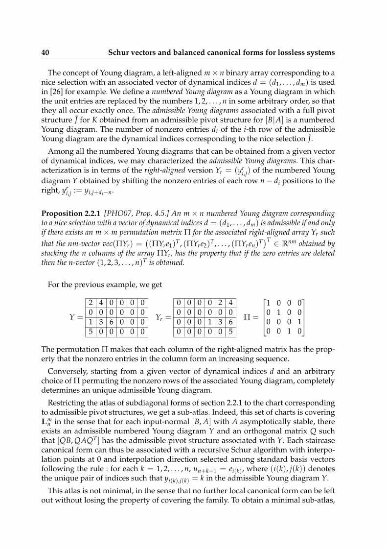
40 Schur vectors and balanced canonical forms for lossless systems
The concept of Young diagram, a left-aligned m× n binary array corresponding to anice selection with an associated vector of dynamical indices d = (d1, . . . , dm) is usedin [26] for example. We define a numbered Young diagram as a Young diagram in whichthe unit entries are replaced by the numbers 1, 2, . . . , n in some arbitrary order, so thatthey all occur exactly once. The admissible Young diagrams associated with a full pivotstructure J for K obtained from an admissible pivot structure for [B|A] is a numberedYoung diagram. The number of nonzero entries di of the i-th row of the admissibleYoung diagram are the dynamical indices corresponding to the nice selection J.
Among all the numbered Young diagrams that can be obtained from a given vectorof dynamical indices, we may characterized the admissible Young diagrams. This char-acterization is in terms of the right-aligned version Yr = (yr
i,j) of the numbered Youngdiagram Y obtained by shifting the nonzero entries of each row n− di positions to theright, yr
i,j := yi,j+di−n.
Proposition 2.2.1 [PHO07, Prop. 4.5.] An m× n numbered Young diagram correspondingto a nice selection with a vector of dynamical indices d = (d1, . . . , dm) is admissible if and onlyif there exists an m×m permutation matrix Π for the associated right-aligned array Yr suchthat the nm-vector vec(ΠYr) =
((ΠYre1)T, (ΠYre2)T, . . . , (ΠYren)T)T ∈ Rnm obtained by
stacking the n columns of the array ΠYr, has the property that if the zero entries are deletedthen the n-vector (1, 2, 3, . . . , n)T is obtained.
For the previous example, we get
Y =
2 4 0 0 0 00 0 0 0 0 01 3 6 0 0 05 0 0 0 0 0
Yr =
0 0 0 0 2 40 0 0 0 0 00 0 0 1 3 60 0 0 0 0 5
Π =
1 0 0 00 1 0 00 0 0 10 0 1 0
The permutation Π makes that each column of the right-aligned matrix has the prop-erty that the nonzero entries in the column form an increasing sequence.
Conversely, starting from a given vector of dynamical indices d and an arbitrarychoice of Π permuting the nonzero rows of the associated Young diagram, completelydetermines an unique admissible Young diagram.
Restricting the atlas of subdiagonal forms of section 2.2.1 to the chart correspondingto admissible pivot structures, we get a sub-atlas. Indeed, this set of charts is coveringLm
n in the sense that for each input-normal [B, A] with A asymptotically stable, thereexists an admissible numbered Young diagram Y and an orthogonal matrix Q suchthat [QB, QAQT] has the admissible pivot structure associated with Y. Each staircasecanonical form can thus be associated with a recursive Schur algorithm with interpo-lation points at 0 and interpolation direction selected among standard basis vectorsfollowing the rule : for each k = 1, 2, . . . , n, un+k−1 = ei(k), where (i(k), j(k)) denotesthe unique pair of indices such that yi(k),j(k) = k in the admissible Young diagram Y.
This atlas is not minimal, in the sense that no further local canonical form can be leftout without losing the property of covering the family. To obtain a minimal sub-atlas,
2.3 Perspectives 41
one has to choose one of the local canonical forms for each d ∈ D(m, n). One possiblechoice is the unique permutation for which the permuted dynamical indices form anon-increasing sequence, while the order of the rows which have the same dynamicalindex is kept the same. With hindsight, one can say that this particular choice to obtaina minimal atlas for continuous-time lossless systems was used in [30].
The number of charts in the various atlases are
subdiagonal forms straicase forms minimal atlas
mn ∑minm,n`=1 `!
(m`
)(n− 1`− 1
) (m + n− 1
m− 1
)To demonstrate the structure of the charts that constitute the various atlases, a simple
example (m = 2, n = 3) is presented in Figure 2.1. The charts marked with a ∗ forma minimal atlas. A Young diagram representation is also used for subdiagonal butnon-staircase forms. In this case, the numbering in the Young diagram specifies thepivot structure of [B A] according to Theorem 2.2.4 but gives no information on thecontrollability matrix.
2.3 Perspectives
In this chapter, we have described (structured) canonical forms which can be para-metrized using Schur vectors. This approach combines the practical advantages ofstate-space representations with the efficiency and simplicity of Schur analysis. It hasa wide range of applications, most of which have not yet been explored.
In [31] the structure of the canonical form was used to show that the set of losslessfunctions of order ≤ n with the topology induced by H2 has the structure of an 2n + 1hypersphere S2n+1. The subspace of lossless systems of order ≤ k < n appears as anembedded hypersphere. Looking at the Hessenberg form (2.2) parametrized by thesequence of Schur parameters, the situation can be analyzed as follows: if the normof some Schur parameter, say γj, goes to 1, the corresponding pivot κj goes to 0 andthe dynamic matrix A then presents a diagonal block-structure with a unitary lowerblock. The realization is no more minimal, but represents a n− j order (still lossless)system. The lossless systems of order < n appear as boundary points in L1
n and theHessenberg structure can be used for model reduction purposes.
In the MIMO case, because of the non-trivial manifold structure of Lmn , a pivot in
a local subdiagonal form can be zero for two completely different reasons: either thelocal chart is not adapted or the underlying system fails to be controllable which is theboundary case. To say it differently, the boundary of a chart (local subdiagonal chart)is mostly composed by systems of order n, for which another chart should be used,and some of order < n, which are boundary points of the manifold. It would be veryhelpful, both for identification and model reduction purposes, to better understand thetopological structure of the set of m × m lossless systems of order ≤ n. Subdiagonalforms could bring some insights in this study. They could also provide simple methodsfor model order reduction for lossless systems as well as other classes of systems,

42 Schur vectors and balanced canonical forms for lossless systems
Chart [B|A] Pivot structure Young Diagram Canonical form
(e1, e1, e1)
+ ∗ ∗ ∗ ∗0 ∗ + ∗ ∗0 ∗ 0 + ∗
1, 3, 4 1 2 3staircase∗
(e1, e1, e2)
∗ + ∗ ∗ ∗+ 0 ∗ ∗ ∗0 0 ∗ + ∗
2, 1, 4 2 31 subdiagonal
(e1, e2, e1)
+ ∗ ∗ ∗ ∗0 + ∗ ∗ ∗0 0 + ∗ ∗
1, 2, 3 1 32 staircase
(e2, e1, e1)
+ ∗ ∗ ∗ ∗0 ∗ + ∗ ∗0 + 0 ∗ ∗
1, 3, 2 1 23 staircase∗
(e2, e2, e1)
+ ∗ ∗ ∗ ∗0 + ∗ ∗ ∗0 0 ∗ + ∗
1, 2, 4 12 3 subdiagonal
(e1, e2, e2)
∗ + ∗ ∗ ∗∗ 0 + ∗ ∗+ 0 0 ∗ ∗
2, 3, 1 31 2 staircase∗
(e2, e1, e2)
∗ + ∗ ∗ ∗+ 0 ∗ ∗ ∗0 0 + ∗ ∗
2, 1, 3 21 3 staircase
(e2, e2, e2)
∗ + ∗ ∗ ∗∗ 0 + ∗ ∗∗ 0 0 + ∗
2, 3, 4 1 2 3 staircase∗
Figure 2.1: Subdiagonal canonical forms for m = 2, n = 3.
2.3 Perspectives 43
based on this observation: if [B|A] is in subdiagonal pivot form and we truncate thelast n − i rows and columns, we again have a controllable pair in subdiagonal pivotform.
One of the main practical reasons for studying atlases of charts was that of iterativeoptimization algorithms using differential tools in the MIMO case. Even if our pref-erence bears on infinite and flexible atlases (see Chapter 3), a finite atlas of structuredcanonical forms could present some interest. The issue of selecting a better chart whenswitching becomes necessary and of monitoring the conditioning of a chart are funda-mental in this connection. For the atlas of subdiagonal canonical forms, the algorithmof section 2.2.2 provides a chart for a given system. However, we don’t know whatcould be a good choice of the non-zero vector (the pivot column) at each step of thealgorithm. This essential question may have different answers from a model reductionor an optimization perspective. A chart selection algorithm is missing for the atlas ofstaircase forms and will be highly desirable.
Subdiagonal pivot structures could be even more interesting in the continuous-timesetting. Real world systems are often described by means of realization with a par-ticular structure in which the physical parameters are displayed (see section 3.4). Insome applications, subdiagonal forms could offer an easy connection between op-timization parameters and physical parameters. In the SISO case, the single subdi-agonal canonical form is the well-known Schwarz-Ober form in which the dynamicmatrix A is tridiagonal. It can be parametrized by the n positive pivots [52]. It is pos-sible to interpret these parameters as interpolation values in a recursive Schur algo-rithm, but the interpolations values must be taken at ∞ which belongs to the analyt-icity boundary in continuous-time [OHP08]. Multivariable lossless systems can anal-ogously be parametrized using interpolation data on the imaginary line [4, Chap. 21].However, the overlapping subdiagonal canonical forms are not easily recovered fromthese parametrizations. It must be noticed that vanishing moments, diagonal Markovparameters, can be interpreted in term of boundary interpolation conditions. Bound-ary interpolation sounds a promising tool and its use in the representation of bothcontinuous-time and discrete-time systems is under investigation.

44 Schur vectors and balanced canonical forms for lossless systems

Chapter 3
Rational H2 approximation and losslessmutual encoding
Rational approximation was the first topic I studied some twenty years ago. It is at theorigin of my interest for lossless functions and their parametrizations.
Since finite order LTI systems and their rational transfer functions are the most usedmodels in system theory, rational approximation is at the heart of modeling problems.The challenge is to select a model that is close enough to a physical system and yetsimple enough to be studied analytically. Modeling is thus at the origin of a fertile in-teraction between rational approximation methods and system theory. A great num-ber of methods have been proposed in the literature, that divide into two main groups:projection methods and optimization methods (see [12] for a nice oriented historicalsurvey).
Among these methods, rational approximation in the Hardy space H2 presents anumber of interesting features. Assuming a transfer function belongs to H2 corre-sponds to a stability condition for the underlying physical system: a bounded energyinput produces a bounded output. The Hardy space H2 possesses a very rich structurewhich combines analyticity properties and an Hilbert space framework. However, H2rational approximation is a difficult non-linear problem due to the complexity of theset approximants (rational matrices of fixed order) and the existence of many localminima.
A specific approach has been developed at INRIA to cope with this problem, whichis based on the following points
• the optimization range is reduced to the set of lossless functions,
• an atlas of chart is used to parametrize the set of lossless functions.
The exposition here is definitely application oriented, so that the emphasis will be puton the effective implementation of the method. It is based on state-space formulas anda suitable atlas of chart which was presented in [MO07].

46 Rational H2 approximation and lossless mutual encoding
3.1 The rational approximation problem
The L2-norm of a matrix-valued function F(z) whose entries belong to L2(T) is givenby
‖F‖22 =
12π
Tr∫ 2π
0F(eit)F(eit)
∗dt.
The rational approximation problem we consider is, given a matrix-valued functionF(z) ∈ Hp×m
2 , to minimize the L2 distance to the set of rational functions in Hp×m2 of
McMillan degree less than or equal to n.
First remark that any solution H must satisfy H(∞) = F(∞). Thus, we may restrict
our study to the case of strictly proper transfer functions, that is to the space (Hp×m2 )
⊥.
A number of qualitative results are available which assert that the problem is well-posed and pave the way to convergent algorithms. It was proved in [5] that the globalminimum of the L2 criterion does exist, as well as the normality property: if F(z) is not ofMcMillan degree strictly less than n, then the best approximant H(z) at order less thanor equal to n has effective order n, so that the problem can now be stated as:
Rational approximation problem. Given F(z) ∈ (Hp×m2 )
⊥, find H(z) such that
H = argminH∈Ξn‖F− H‖2
2 (3.1)
whereΞn = H ∈ (Hp×m
2 )⊥
, deg H = n
is the set of rational strictly proper stable transfer functions of exact degree n.
The following consistency result should also be mentioned: if F(z) has McMillan de-gree n, then the only local minima (and even the only critical point) of the L2 criterionis F(z) itself [BO98].
The present approach was first proposed in the SISO case [BCO91] and then in theMIMO case [FO98]. The first step is the elimination of the linear variable by means ofthe Douglas-Shapiro-Shields factorization (Theorem 1.1.5). Any rational matrix func-
tion H(z) ∈ (Hp×m2 )
⊥can be written in the form
H(z) = C(z)G(z),
where G(z) is lossless of McMillan degree n and C(z) ∈ Hp×m2 . Any approximant H(z)
of F(z) thus minimizes the distance from F(z) to the vector space
Vec(G) = H ∈ (Hp×m2 )
⊥; H = C G, C ∈ Hp×m
2 .
The Projection theorem in a Hilbert space asserts that H(z) is completely determinedby G(z) as the orthogonal projection of F(z) onto Vec(G). Equivalently, C(z) is theorthogonal projection of F(z)G](z) onto Hp×m
2 , C(z) = π+(FG]). In least-square op-timization and using a state-space formulation, this elimination step is classical and

3.2 Nudelman interpolation and lossless mutual encoding 47
known under the name of Separable Least Square. It presents some important advan-tages: the dimension of the parameters space is reduced and mostly, lossless functionsenter the picture. The rational approximation problem is then to minimize the criterion
ψn : G 7→ ‖F− π+(FG])G‖2 (3.2)
over the set Lmn \Um the right quotient of the set of m×m lossless functions of McMil-
lan degree n by unitary constant matrices.
The second step is to find a clever parametrization of the set Lmn and its right quo-
tient Lmn \Um. In order to use differential tools (as a gradient algorithm) to solve this
optimization problem, an atlas of charts happens to be the desirable representation.Over the years, different atlases of charts have been experimented and implemented.The first one was the atlas derived form the tangential Schur algorithm constructed in[1]. A polynomial representation of lossless matrices were used as described in [FO98]and implemented in the software Hyperion [29]. However, a state-space representa-tion is often preferred for computations and the balanced canonical forms of section2.1 were used in the software RARL2 [MO04]. However, the natural framework forthis atlas is that of complex valued functions. In particular, an adapted chart, that isa chart centered at a given lossless function requires complex interpolation points, its(possibly complex) poles (see section 2.1).
However, physical systems are often real-valued and their transfer functions T(z)are real, that is, they satisfy the relation T(z) = T(z). It must be mentioned that the bestcomplex approximation of a real function may fail to be real. For example the functionf (z) = 1/z3 − 1/z admits three minima: a real one and two complex, which achievethe best relative error. In the next section, we propose an atlas which better suits therepresentation of real lossless functions. It is based on the more general Nudelmaninterpolation problem (see section 1.3.3).
3.2 Nudelman interpolation and lossless mutual encod-ing
We first built an atlas of chart for the set Lpn. To this end, we consider the interpolation
problem (see section 1.3.3) now stated for lossless functions: given an observable pair(U, W), where W is n× n stable, find all the lossless function G(z) ∈ Lm
n satisfying theinterpolation condition
12iπ
∫T(zI −W∗)−1U∗G](z) dz = V∗. (3.3)
Note that two equivalent triples (W, U, V) and (TWT−1, UT−1, VT−1) yield the sameinterpolation condition (3.3). Thus, we may assume the observable pair (U, W), W isstable, to be output normal :
U∗U + W∗W = I. (3.4)

48 Rational H2 approximation and lossless mutual encoding
By Theorem 1.3.1, if the solution P to the Stein equation (1.39) is positive definite,then the set of all lossless solutions G(z) of McMillan degree n of (3.3) is given by
G(z) ∈ Lmn ; G = TΘW,U,V H(G0), G0 constant unitary matrix
where ΘW,U,V is the J-inner matrix (1.40) with ν = 1 and H is a right constant J-unitarymultiplier, that can be freely chosen.
A chart of Lmn is thus attached to an output normal pair (U, W), and a lossless func-
tion G(z) belongs to the domain VU,W of this chart if and only if the solution P to theStein equation (1.39) is positive definite. The coordinate map is
φU,W : G ∈ VU,W → (G0, V).
The matrix H may depend on the interpolation triple (W, U, V). In this case we shallrequire H(W, U, V) to be differentiable with respect to V and to satisfy the relation[
Λ 00 Π
]H(W, U, V)
[Λ∗ 00 Π∗
]= H(W, ΛU, ΠV) (3.5)
for any unitary matrices Λ and Π. This equality ensures that the quotient Lmn \Um can
be perform within each chart by fixing G0.The matrix H and unitary matrices U and V can be constructed following the approachof section 2.1 so that a balanced canonical form is computed by the multiplicativeformula (2.11) in which d = n. However, in the present case the balanced canonicalform can be obtained directly and nicely interpreted. The interpolation value V in (3.3)as a very simple state-space formulation. An analog formula has also been derived incontinuous-time in [28].
Proposition 3.2.1 [MO07, Prop. 4] Let (U, W) be an output normal pair, W stable, and letG(z) = D + C(zIn − A)−1B be a balanced realization of G(z) ∈ Lm
n . Let Q be the uniquesolution to the Stein equation
Q− AQW = BU (3.6)
Then, the interpolation value V in (3.3) and the associated solution P to the Stein equation(1.39) are given by
V = DU + CQW (3.7)
P = Q∗Q. (3.8)
Formula (3.7) is easily established and can be rewritten with (3.6) in a matrix form[D CB A
] [U
QW
]=[
VQ
]. (3.9)
The realization of G(z) being balanced by assumption, we get
U∗U + W∗QQ∗W = V∗V + Q∗Q,
so that Q∗Q = P, the unique solution of (1.39).

3.2 Nudelman interpolation and lossless mutual encoding 49
Under the assumption P > 0 and thus K = V∗V + P positive definite, we would liketo reverse the process and specify a unique way to compute a balanced realization ofG(z) from the interpolation matrix V and a constant unitary matrix (the analog of G0in the LFT representation).
We first fix the square root Q of P to be the (uniquely defined) Hermitian square root,Q = P1/2, and we use it to normalize the interpolation data
(W, U, V) 7→ (W, U, V) = (QWQ−1, UQ−1, VQ−1) (3.10)
Then, equation (3.9) yields[VI
]∗ [ D CB A
] [UW
]= V∗V + I.
Using the Hermitian square root K1/2 of K = V∗V + I, we get[VK−1/2
K−1/2
]∗ [ D CB A
] [UK−1/2
WK−1/2
]= I.
For any unitary completions U , V of these orthonormal columns,
U =[
UK−1/2 ∗WK−1/2 ∗
], V =
[VK−1/2 ∗K−1/2 ∗
]we have that
V∗[
D CB A
]U =
[I 00 D0
](3.11)
for some unitary matrix D0.
Now, the unitary completions U and V have to be specified. In [MO07] the matrix Vis chosen accordingly to Proposition 1.3.2 in which J = I and ν = −1 :
V =[
V(I + V∗V)−1/2 (I + VV∗)−1/2
(I + V∗V)−1/2 −V∗(I + VV∗)−1/2
]. (3.12)
For the matrix U , another method is used which makes use of a Cholesky factoriza-tion, and has been implemented in the software RARL2.First remark that when D0 = I and V = 0 we get[
D CB A
]=[∗ ∗
U∗ W∗
],
whence the idea to attach a chart to a unitary balanced realization
Ω = (W∗, U∗, Y∗, X∗) (3.13)
rather than just an output normal pair (W, U).
The matrix U is then computed from Ω as follows:

50 Rational H2 approximation and lossless mutual encoding
• perform a state isomorphism with matrix Q = P1/2:
(W, Y, U, X) −→ (W, Y, U, X) = (QWQ−1, QY, UQ−1, X).
• compute a Cholesky factorization of the matrix[K LL∗ N
]=[
U XW Y
]∗ [U XW Y
]. (3.14)
using the well-known formula [18, Sec. 0.2], we get[K LL∗ N
]=
[I 0
L∗K−1 I
] [K 00 Z−1
] [I K−1L0 I
]=
[K1/2 K−1/2L
0 Z−1/2
]∗ [K1/2 K−1/2L0 Z−1/2
]where Z−1 = N − L∗K−1L can be computed by inverting the matrix (3.14) [18,Formula (0.8)].
The matrix
U =[
U XW Y
] [K−1/2 −K−1LZ1/2
0 Z1/2
](3.15)
is then a unitary completion of the orthonormal columns of[UK−1/2 WK−1/2
]T.
The matrices K, L and Z are given by
L = U∗X + W∗Y (3.16)K = U∗U + W∗W = I + V∗V (3.17)Z = X∗X + Y∗Y. (3.18)
and it is easily checked that K and Z are positive definite.
Proposition 3.2.2 [MO07, Prop. 5] A lossless function G(z), given by a balanced realization(A, B, C, D), is in the domain DΩ of the chart associated with Ω = (W∗, U∗, Y∗, X∗) if andonly if the solution Q to the Stein equation (3.6) is positive definite. A realization R is incanonical form with respect to this chart if and only if the solution Q to (3.6) is P1/2, P beinga solution of (1.39).
The coordinate map isφΩ : G(z) ∈ DΩ → (D0, V),
in which V and D0 are computed as follows :
• first compute V and Q by (3.7) and (3.6)
• then compute P = Q∗Q and U and V as in (3.15) and (3.12)

3.3 RARL2 : a rational approximation software 51
• finally compute T = QP−1/2 and (A, B, C, D) = (T−1AT, T−1B, CT, D) a bal-anced realization for G(z) in canonical form. Then D0 is given by
V∗[
D CB A
]U =
[I 00 D0
]. (3.19)
The balanced realization Ω = (W∗, U∗, Y∗, X∗) defines a lossless function
GΩ(z) = X∗ + U∗(zIn −W∗)−1Y∗ ∈ Lmn . (3.20)
Since two similar balanced realizations provide the same chart up to a rotation in theparameters space, the chart is in fact attached to an element of Lm
n which explains thedenomination lossless mutual encoding.
The solution Q of (3.6) has the following integral representation ([4, Th. A.2.2.])
Q =1
2iπ
∫T(z I − A)−1BU(I − z W)−1dz.
This formula can be interpreted as a matrix-valued inner product
Q =⟨(zI − A)−1B, (zI −W∗)−1U∗
⟩defined on the left Hilbert module of n×m square integrable matrix-valued functionson the unit circle [10]. Since the pairs (W∗, U∗) and (A, B) are input normal, theirdistance in the norm associated with the matrix-valued inner product is
‖|(zI − A)−1B− (zI −W∗)−1U∗‖| = 2I −Q−Q∗.
Hence, the quality of a chart can be estimated by computing m(P) ∈]0, 1]:
m(P) = inf|λ|, λ eigenvalue of P).
The closer m(P) is to 1, the better is the chart, the best choice being P = I. This choiceprovides us with an adapted chart.
Proposition 3.2.3 (Adapted chart) [MO07] The chart associated with a balanced realiza-tion Ω = (A, B, C, D) of G(z) is an adapted chart for G(z), i.e. the interpolation matrix V in(3.7) is the zero matrix and D0 = I.
If φΩ(G) = (D0, V) and Σ is a constant unitary matrix, then φΩ(ΣG) = (ΣD0, ΣV).An atlas for the (left) quotient space Lm
n \Um is thus obtained by fixing D0 within eachchart.
3.3 RARL2 : a rational approximation software
The Matlab based software RARL21 solves the minimization problem (3.1) for a func-tion F(z) given in one of the following forms
1The software RARL2 is described in [MOHP02] and available on the web pagehttp:www-sop.inria.fr/apics/RARL2/rarl2-eng.html.

52 Rational H2 approximation and lossless mutual encoding
(1) a realization F(z) = D + C(zIN −A)−1B
(2) Fourier coefficients F(z) = ∑Nj=0 Fjz−j.
It is mostly a model reduction tool. Pointwise values on the circle
F(eiθj), j = 1, . . . , N
can also be handled, but in this case the L2-norm is replaced by a least-square criterion.Then, the result is not guaranteed and very dependent on the data. When the data isband-limited a first completion step is highly desirable (see section 3.4). In this connec-tion, other representations of functions, using alternative basis of L2(T) as orthogonalrational functions [12], could better suit the completion issue.
The implementation is based on a state space representation (A, B, C, D) of LTI stablesystems approximants. The concentrated criterion (3.2) is thus defined on the set oflossless functions or equivalently input normal pairs (A, B). It is computed, as well asthe gradient, using state-space formulas.
Let H(z) = D + Γ(zI − A)−1B with (A, B) input normal. The error F− H has real-ization
A =[A 00 A
], B =
[BB
], C =
[C −Γ
], D = 0,
and L2 norm‖F− H‖2
2 = Tr(CWcC∗
),
where Wc is the reachability gramian of the error. Fixing A and B, the L2 error is mini-mal for Γ = CW12, where W12 is the submatrix of Wc solution to
AW12A∗ + BB∗ = W12,
and the concentrated criterion is
J(A, B) = ‖F‖22 − Tr (CW12W∗12C∗) . (3.21)
Let W21 be the solution of the Lyapunov equation
A∗W21A− Γ∗C = W21, Γ = CW12
The gradient of the concentrated criterion can then be computed as
∆J(A, B).(∂A, ∂B) = 2 Re (Tr (W21AW12 ∂A∗)) + 2 Re (Tr (W21B ∂B∗)) (3.22)
The software divides into two libraries
• arl2lib contains all the computations concerning the L2 criterion.The functions arl2SS and arl2COEFF compute the criterion and the gradientwhen the function is given by a realization and Fourier coefficients respectively.
• boplib is concerned with the parametrization of lossless functions (balanced out-put pairs) by means of the lossless mutual encoding method described in section3.2. It also provides a minimization process which could handle any criteriondefined over the manifold Lm
n \Um.
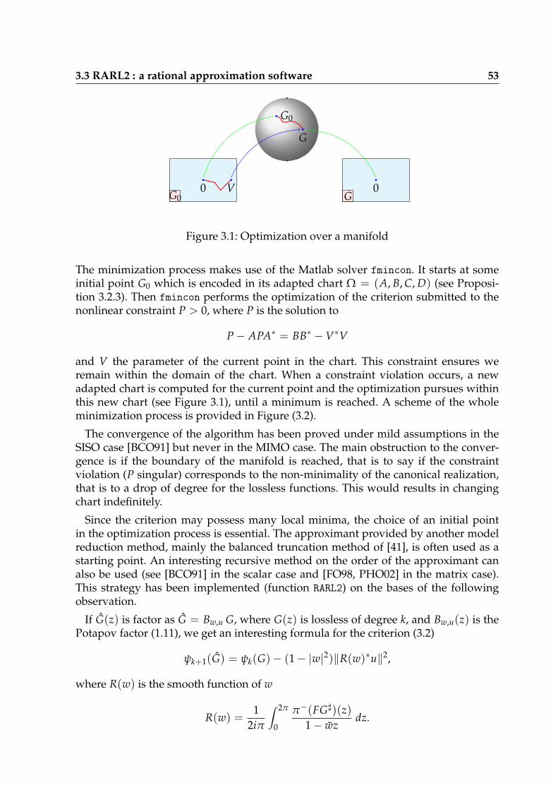
3.3 RARL2 : a rational approximation software 53
G0
G
0G0
VG
0
Figure 3.1: Optimization over a manifold
The minimization process makes use of the Matlab solver fmincon. It starts at someinitial point G0 which is encoded in its adapted chart Ω = (A, B, C, D) (see Proposi-tion 3.2.3). Then fmincon performs the optimization of the criterion submitted to thenonlinear constraint P > 0, where P is the solution to
P− APA∗ = BB∗ −V∗V
and V the parameter of the current point in the chart. This constraint ensures weremain within the domain of the chart. When a constraint violation occurs, a newadapted chart is computed for the current point and the optimization pursues withinthis new chart (see Figure 3.1), until a minimum is reached. A scheme of the wholeminimization process is provided in Figure (3.2).
The convergence of the algorithm has been proved under mild assumptions in theSISO case [BCO91] but never in the MIMO case. The main obstruction to the conver-gence is if the boundary of the manifold is reached, that is to say if the constraintviolation (P singular) corresponds to the non-minimality of the canonical realization,that is to a drop of degree for the lossless functions. This would results in changingchart indefinitely.
Since the criterion may possess many local minima, the choice of an initial pointin the optimization process is essential. The approximant provided by another modelreduction method, mainly the balanced truncation method of [41], is often used as astarting point. An interesting recursive method on the order of the approximant canalso be used (see [BCO91] in the scalar case and [FO98, PHO02] in the matrix case).This strategy has been implemented (function RARL2) on the bases of the followingobservation.
If G(z) is factor as G = Bw,u G, where G(z) is lossless of degree k, and Bw,u(z) is thePotapov factor (1.11), we get an interesting formula for the criterion (3.2)
ψk+1(G) = ψk(G)− (1− |w|2)‖R(w)∗u‖2,
where R(w) is the smooth function of w
R(w) =1
2iπ
∫ 2π
0
π−(FG])(z)1− wz
dz.

54 Rational H2 approximation and lossless mutual encoding
sys0
bopAllpassFactor
losslessfactor
W2CSP SP2X
chart Ωparam X
FUNarl2Mono
data
NONLCONbopSPModulus
optimoptions
fmincon
errorparam X
bopchangechart chart Ωparam X
report
const. saturated
Figure 3.2: Minimization process in RARL2
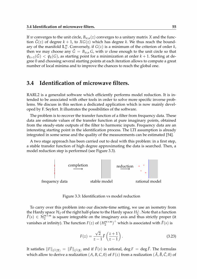
3.4 Identification of microwave filters. 55
If w converges to the unit circle, Bw,u(z) converges to a unitary matrix X and the func-tion G(z) of degree k + 1, to XG(z) which has degree k. We thus reach the bound-ary of the manifold Lm
n . Conversely, if G(z) is a minimum of the criterion of order k,then we may choose any G = Bw,u G, with w close enough to the unit circle so thatψk+1(G) < ψk(G), as starting point for a minimization at order k + 1. Starting at de-gree 0 and choosing several starting points at each iteration allows to compute a greatnumber of local minima and to improve the chances to reach the global one.
3.4 Identification of microwave filters.
RARL2 is a generalist software which efficiently performs model reduction. It is in-tended to be associated with other tools in order to solve more specific inverse prob-lems. We discuss in this section a dedicated application which is now mainly devel-oped by F. Seyfert. It illustrates the possibilities of the software.
The problem is to recover the transfer function of a filter from frequency data. Thesedata are estimate values of the transfer function at pure imaginary points, obtainedfrom the steady-state outputs of the filter to harmonic inputs. Frequency data are aninteresting starting point in the identification process. The LTI assumption is alreadyintegrated in some sense and the quality of the measurements can be estimated [54].
A two stage approach has been carried out to deal with this problem: in a first step,a stable transfer function of high degree approximating the data is searched. Then, amodel reduction step is performed (see Figure 3.3).
frequency data
completion
stable model
reduction + +
++
rational model
Figure 3.3: Identification vs model reduction
To carry over this problem into our discrete-time setting, we use an isometry fromthe Hardy spaceH2 of the right half-plane to the Hardy space H⊥2 . Note that a functionF(s) ∈ Hm×m
2 is square integrable on the imaginary axis and thus strictly proper (it
vanishes at infinity). The function F(z) of (Hm×m2 )⊥ which is associated with F(s) is
F(z) =√
2z− 1
F(
z + 1z− 1
). (3.23)
It satisfies ‖F‖L2(T) = ‖F‖L2(I) and if F(s) is rational, deg F = deg F. The formulaswhich allow to derive a realization (A, B, C, 0) of F(z) from a realization (A, B, C, 0) of

56 Rational H2 approximation and lossless mutual encoding
F(s) and reciprocally are completely symmetric:
C = CA = −(I − A)−1(I + A)B = (I − A)−1B
C = CA = −(I − A)−1(I + A)B = (I − A)−1B
(3.24)
The data on the imaginary axis can be sent on the unit circle via the Mobius transfor-mation iwk 7→ iwk+1
iwk−1 and we get an equivalent problem in the framework of the disk(see Figure 3.4). However, if the original system fails to be strictly proper, then thedirect feedthrough (value at infinity of the transfer function) must be evaluated.
frequency data
completion
stable model
reduction ++++
rational model
Figure 3.4: Two steps identification in discrete-time
Since the data are usually band-limited, this problem is not well-posed and a met-ric constraint must be imposed outside the bandwidth. This completion problem is adifficult task, for which a lot of methods have been proposed, whose efficiency mostlydepend on the quality of the data and require some engineering ability. The methodsdivide in two classes, interpolation methods among which boundary Nevanlinna-Pickinterpolation algorithms sounds interesting [14], and approximation methods more in-clined to take into account the quality of the data.
For the identification of microwave filters, we chose the approximation approachand solved a bounded extremal problem. The whole process is described in [BGL+98].The model reduction step is then performed by the software RARL2 as explained insection 3.3. The microwave filters that we consider are used in telecommunicationsatellites for channel multiplexing. A longstanding cooperation with the space agencyCNES resulted in a dedicated software PRESTO-HF [60] that wraps RARL2 into apackage which is now fully integrated in the design and tuning process. In Figure3.5, a 8th order model of a MIMO 2× 2 microwave filter is shown, obtained from 800pointwise data.
3.5 More applications
The rational approximation method and the software described in this chapter havebeen used in several different situations which demonstrates the adaptability of thisapproach.

3.5 More applications 57
Figure 3.5: Bode diagram of the data and the approximant at order 8.
3.5.1 Localization of dipolar sources in electroencephalography.
This research is conducted by J. Leblond and L. Baratchart from the APICS-INRIAteam. From measurements by electrodes of the electric potential u(z) on the scalp, theproblem is to recover a distribution of m pointwise dipolar current sources Ck ∈ R3
with moments pk ∈ R3 located in the brain (modeling the presence of epileptic foci).The head is modeled as a set of three spherical nested regions (brain, skull, scalp) andin each region constant conductivities are assumed. A macroscopic model and quasi-static approximation of Maxwell-equations are used to describe the spacial behaviorof u(z). In the brain, the electric potential u(z) assumes the form
u(z) = h(z) +m
∑k=1
< pk, x− Ck >
4π‖x− Ck‖3 ,
where h(z) is harmonic, while the other component (anti-harmonic part ua(z)) bearsthe information on the sources.
The inverse problem can be approach in two steps: get first ua(z) from the data andthen recover the localizations and the moments of the sources from ua(z). Rationalapproximation is involved in this second step [6] and performs on planar sections (seeFigure 3.6).
Note that ua(z) is not rational and only has singularities. However, the restrictions

58 Rational H2 approximation and lossless mutual encoding
Figure 3.6: Rational approximation on planar sections
fp(z) of ua(z)2 to planar sections Γp of the brain possesses triple poles and singularitiesat the same location. These singularities are strongly and explicitly linked with thesources, and the poles of the best L2 rational approximations to fp on Γp accumulateto these singularities [7] (see Figure 3.7).
Figure 3.7: Localization of sources: the singularities (green) are aligned and the sources(black) correspond to the maximum modulus. The rational approximations (red) ac-cumulate to these singularities.
One of the advantages of this method is that it does not require the a priori knowl-edge of the exact number of sources. If the order of the approximation is larger thanthe number of sources, the extra poles accumulate to the boundary of the domain Γp.For this application, the software RARL2 has been modified to impose triple poles forthe approximant. This was an easy trick thanks to the flexibility of the parametrizationof section 3.2.

3.5 More applications 59
3.5.2 Multi-objective control.
In [57], revisited in a chain-scattering perspective in [DMO05], it is shown that if thepair (C, A) of the Youla parameter Y(z) = D + C(zI − A)−1B is fixed, then the searchover the parameters (B, D) can be reduced to an efficiently solvable LMI problem.Limiting the search of the parameter Y(z) to the FIR form
Y(z) = Y0 + Y11z
+ . . . + Yp1zp
provides solutions to the multi-objective control problem. However, this is also themain limitation of the approach as high order expansions might be necessary, due no-tably to the fact that the poles structure is fixed through the pair (C, A). Such a draw-back can be avoided if the search is performed over all the parameters Y(z) of fixedMcMillan degree. This can be done using the atlas of section 3.2 to parametrize the cor-responding pairs (C, A). The modularity of RARL2 allows to use this parametrization(library boplib) to optimize a different criterion. This algorithm for multi-objectivecontrol has been implemented by M. Bordier and J.P. Marmorat.
3.5.3 Wavelets approximation
Figure 3.8: Daubechies wavelet db7 (blue) and its degree 8 rational approximation(green).
This application of our rational approximation methods to orthogonal wavelets wasproposed by R. Peeters. The problem is to implement wavelets in analog circuits inview of medical signal processing applications. A dedicated method has been devel-oped [38] based on an L2-approximation of the wavelet by the impulse response of a

60 Rational H2 approximation and lossless mutual encoding
stable, causal, low order filter. However, this method fails to find an accurate and suf-ficiently small order approximation in some difficult cases (Daubechies wavelets db7and db3).
The idea was to use the software RARL2 to perform a model reduction on an ac-curate high order (100-200) approximation. However, an admissibility condition forwavelets is that the integral of a wavelet equals zero, which means that it has a van-ishing moment of order 0. The low order approximation is still required to have anintegral zero, otherwise undesired bias will show up when the wavelet is used in anapplication. We thus had to adapt a version of the RARL2 software to address thisconstraint. Since we are dealing with a quadratic optimization problem under a linearconstraint, this can be solved analytically. We could thus reformulate the problem ofL2-approximation subject to this constraint into an optimization problem over the classof lossless systems. This could be handled by the software with only minor changesand we were able to perform an accurate approximation of order 8 for db7 (Figure 3.8).
3.6 Perspectives.
The examples presented in section 3.5 show the wide range of applicability of themethod and suggest a number of improvements as well as new lines of research. Inthe applications to multi-objective control and wavelet approximation, the criterionhas been modified to address a different linear constraint.
In the inverse problem of source recovery, the function to be approximated is notrational but non integer rational (it involves fractional powers). A interesting topic forfuture research would be the approximation by non integer rational functions. Frac-tional (or non integer) systems and fractional orthonormal basis are active domain ofresearch which could be connected in some way to our works. However, I have noknowledge in this domain, and this is presently a very prospective subject.
At contrary, enforcing passivity in rational approximation tools is already underinvestigation. Passive devices play an important role in a lot of application areas:telecommunication, chemical process control, economy, biomedical processes. Net-work simulation software packages (as ADS or SPICE) require passive models for theircomponents. However, enforcing passivity while identifying a model from (band lim-ited) frequency data is still an open and challenging problem. The current approachesare mostly ”ad hoc” methods. The possibility to handle this problem using the approx-imation techniques developed in the APICS team seems promising. Up to now, if thedata comes from a passive system, the passivity of the model is not guaranteed by ourapproach.
The passivity constraint brings new difficulties and rises a number of interestingtheoretical and practical questions, both in the interpolation and in the approximationstep. A passive system has, in case of a scattering representation, a transfer functionwhich is Schur (contractive in the stability domain, see section 1.3). The research couldbe carried out in many directions. The Schur approximation problem should be stud-ied from a theoretical viewpoint: existence of an approximant, behavior of the criterion

3.6 Perspectives. 61
at the boundary of the domain, etc. in order to design a specific algorithm. It must benoticed that approximation from band-limited data becomes a well-posed problemwith the Schur constraint.
The parametrization issue for Schur functions should also be addressed. In V. LunotPHD thesis [48], a parametrization of all strictly Schur rational functions of degree n isconstructed from a multipoint Schur algorithm (the recursive algorithm (1.26) in whichthe interpolation points can be chosen anywhere in the open unit disk), the parametersbeing both the interpolation values and interpolation points. Examples are computedby an L2 norm optimization process and the results are validated by comparison withthe unconstrained L2 rational approximation. Choosing the interpolation points withrespect to the approximated Schur function so as to yield the best convergence pos-sible remains a major open issue. An alternative approach relies on the observationthat a Schur function can be viewed as a sub-block of a lossless function of higher di-mension (see Chapter 4). A parametrization of Schur functions could be deduced fromthat of lossless functions. This approach must be connected to some works on degree-constrained analytic interpolation (see e.g [44, 45]). The use of boundary interpolationcould be proved necessary in this approach to handle functions which are not strictlySchur.

62 Rational H2 approximation and lossless mutual encoding

Chapter 4
Symmetric lossless matrix-valuedextensions of rational contractions
In this chapter, the application we have in mind is the synthesis of resonant filters,mainly microwave or SAW filters used in telecommunication devices. These filters areusually represented by a scattering matrix which is a lossless matrix-valued function.The lossless property is the expression of the conservation law. The reciprocity lawattached to the wave propagation phenomenon makes this matrix symmetric. We arethus interested in an useful description of symmetric lossless matrices in view of filtersdesign applications.
Since the synthesis often concerns the transmission, a submatrix of the scattering ma-trix, we aim at characterizing the sub-matrices of a scattering matrix. Any sub-matrixof a lossless matrix is contractive in the analyticity domain, that is a Schur function(see Section 1.3). Conversely, on which conditions a symmetric Schur matrix S(s) canbe extended into a symmetric lossless one? Without the symmetry requirement, suchan extension is known under the name of Darlington synthesis. This problem has beenwidely studied in the sixties for a circuit synthesis purpose. Darlington proved the ex-istence of such an extension.
The symmetric Darlington synthesis problem has been little studied and the existingsolutions require an important increase of the size of the extension [2]. In [BEGO07],we proved that a Schur matrix S(s) do possess a symmetric lossless extension if andonly if its zeros have even multiplicity. If this condition is not satisfied, given a m×msymmetric Schur matrix S(s) of McMillan degree n, two dual extension problems canbe formulated:
• either we fix the size of the extension to 2m × 2m and we look for a minimaldegree extension,
• or we fix the degree n of the extension and we look for a minimum size extension.
The solutions obtained in [BEGO07, BEGO10] for each of these problems improve sig-nificantly the results in the literature.
In this chapter, we stick to the continuous-time case, which is relevant in filter designapplications, so that our lossless functions are analytic in the right half-plane. The

64 Symmetric lossless matrix-valued extensions of rational contractions
relevant spaces of functions are the Hardy spaces of the right half-plane H2 and H∞.A Schur matrix function belongs to the unit ball ofHm×m
∞ . We set
W∗(s) = W(−s)∗,
the pseudo-Hermitian conjugate of W(s).
4.1 The scalar case
The case where S(s) is a scalar function is easily handled and gives a first illustrationof these problems. If S(s) = p(s)
q(s) is a Schur rational function, then any 2× 2 rationallossless extension can be written in the form [9]
S =1q
[ξ 00 1
] [p∗ −r∗
r p
](4.1)
where ξ ∈ T and r(s) is a polynomial solution to the spectral factorization problem:
rr∗ = qq∗ − pp∗. (4.2)
The Schur property ensures that (4.2) has a solution. Any solution consists in sharingthe conjugate zeros (α,−α) of qq∗− pp∗ between the two factors (the zeros of qq∗− pp∗
on the imaginary axis have even multiplicity). Then, a symmetric extension do existif and only if the zeros of qq∗ − pp∗ have even multiplicities. In this case, it will beessentially unique.
The scattering matrix of a 2-port is of this form. A nice description of these matricesis in term of the polynomial numerators p(s) and r(s). For the matrix (4.1) to be sym-metric, the polynomial r(s) must satisfy r∗ = −ξr. The scattering matrix of a two-portsatisfies in addition S(∞) = I, so that ξ = (−1)n and it can thus be parametrized inthe form
1q
[(−1)n p∗ r
r p
](4.3)
where p(s) ranges over the monic polynomials of degree n and r(s) over the n− 1degree polynomials satisfying the condition r∗ = (−1)n−1r. This form is particularlyinteresting for synthesis purposes [11, 46, 47], since the modulus of the transmissionS12(s) = r(s)
q(s) can only be expressed in terms of p(s) and r(s)
|S12|2 =1
1 + |p|2|r|2
.
From this application viewpoint, completion is closely related to a parametrizationissue: given a part (a block, a column, an element, two numerators) of a lossless matrix,is it possible to rebuilt the whole matrix? In an unique way?

4.2 From Darlington synthesis to symmetric extensions 65
If the zeros of qq∗− pp∗ fail to have even multiplicities, an extension either of higherdegree or of higher dimension must be searched.
We may choose for r(s) the spectral factor whose roots are in the closed left half-plane, unique up to a unit complex number. The extension (4.1) can thus be madesymmetric multiplying it by an appropriate lossless factor (to simplify the writing weset ξ = 1):
S =
− p∗r∗qr
r∗q
r∗q
pq
=
− p∗q
r∗q
rq
pq
[ r∗r 00 1
]. (4.4)
This extension has degree 2n− n0 where n0 is the number of roots of r(s) on the imag-inary axis, counted with multiplicity.
But we can be cleverer and write qq∗ − pp∗ = r21r2r∗2 , where r1(s) is auto-reciprocal
r∗1 = r1, and r2(s) stable with only simple roots. Then, the following extension is sym-metric:
Σ =
− p∗q
r∗2r2
r1r∗2q
r1r∗2q
pq
=
− p∗q
r1r∗2q
r1r2q
pq
[ r∗2r2
0
0 1
].
and in fact it has minimal possible degree.
4.2 From Darlington synthesis to symmetric extensions
Since the notion of a zero is more complicated in the matrix case, the solution of theextension problem will be more involved. The basic extension problem is, given a m×m Schur matrix S(s) of McMillan degree n, to find a 2m× 2m lossless extensions of thesame degree
S =[
S11 S12S21 S
].
The Darlington synthesis can still be obtained in two steps: first compute S21(s) suchthat S21S∗21 = I − SS∗ is a spectral factorization, which makes
[S21 S
]isometric, and
next, compute a lossless extension of it.
Concerning the spectral factorization in the matrix case, we have the following result[67]:
Theorem 4.2.1 (Youla) Let Φ(s) be a rational m×m paraconjugate Hermitian matrix, i.e.
Φ∗(s) = Φ(s),
of normal rank k which is non-negative on the imaginary axis. Then, there exists a m × kmatrix W(s) such that(1) Φ(s) = W(s)W∗(s)
(2) W(s) and its left inverse W(s)−1 are both analytic in Re s > 0.
(3) W(s) is unique up to a constant, unitary k× k matrix multiplier on the right.

66 Symmetric lossless matrix-valued extensions of rational contractions
(4) Any factorization of the form Φ(s) = W(s)W∗(s) in which W(s) is m× k, rational andanalytic in Re s > 0, is given by W(s) = W(s)Q(s) where Q(s) is inner.
W(s) is called the minimum phase spectral factor and W(s) a spectral factor.
Since S(s) is contractive, the matrix Φ(s) = I − S(s)S∗(s) has all the required prop-erties. We assume that the normal rank of Φ(s) is m, which amounts to say that theS(s) is strictly contractive at some point of the imaginary axis. The spectral factors aresquare m×m matrices whose determinants does not vanish identically. They are thusinvertible as rational matrices. We will be mainly interested with those spectral factorsfor which the extension
[S21 S
]has same degree n than S(s) and which are called
minimal spectral factors.
In [42], a state-space construction of all the lossless extensions preserving the McMil-lan degree is presented. It involves the solutions to a Riccati equation which is closelyconnected to the spectral factorization through the Bounded Real Lemma. This lemma[2] asserts that a function given by a minimal realization, S(s) = D + C(sI − A)−1B,is a Schur function strictly contractive at ∞ if and only if there exist P, B, and D21 suchthat
AP + PA∗ + BB∗ + BB∗ = 0PC∗ + BD∗ + BD∗21 = 0DD∗ + D21D∗21 = I
and P is positive definite. Then
S21(s) = D21 + C(sI − A)−1B
is a left spectral factor of I − SS∗.
Let D21 = (I−DD∗)1/2, then B = −(PC∗+ BD∗)D−121 and P is solution to the Riccati
equationR(P) = PγP + αP + Pα∗ + β = 0 (4.5)
where α = A + BD∗(I − DD∗)−1C,β = B(I − D∗D)−1B∗,γ = C∗(I − DD∗)−1C.
Theorem 4.2.2 [42] The following statements are equivalent
(i) S(s) is a Schur function which is strictly contractive at infinity.
(ii) the Riccati equation (4.5) has an Hermitian solution
(iii) All pure imaginary eigenvalues of A have even multiplicity
In this case, there is a one to one correspondence between the Hermitian solutions of (4.5) andthe lossless extensions of S(s) of degree n, whose value at infinity is prescribed by
D21 = (I − DD∗)1/2, D12 = (I − D∗D)1/2, D11 = −D∗

4.2 From Darlington synthesis to symmetric extensions 67
The extension is given by
SP(s) =[
D11 D12D21 D
]+[
CC
](sI − A)−1 [B B
].
Associated with the Riccati equation (4.5), the matrix
A =[−α∗ −γ
β α
]is in fact a (possibly non-minimal) dynamic matrix of (I − SS∗)−1. It is Hamiltonianand its eigenvalues are thus symmetric with respect to the imaginary axis, countingmultiplicities. It satisfies the important similarity relation[
I 0−P I
]A[
I 0P I
]=[−(α + Pγ)∗ −γ
0 α + Pγ
].
The spectrum ofA splits as σ(A) = σ(α + Pγ)∪ σ(−(α + Pγ)∗). It can be verified thatS−1
21 has dynamic matrix α + Pγ while S−112 has dynamic matrix −P(α + Pγ)∗P−1. The
block diagonal form shows us that the matrix P induces a distribution of the zeros ofI − SS∗ (eigenvalues of A) between S12 and S21, in such a way that S12 and S21 haveconjugate zeros with respect to the imaginary axis. This also follows from the nextequality which generalizes in some sense (4.1) to the matrix case [BEGO10]
det S = −det S12 det(S∗21)−1. (4.6)
However, the state-space construction of Theorem 4.2.2 requires the condition S(∞)strictly contractive and symmetric realizations to address the symmetric extensionproblem. However, the scattering matrix of a m-port usually satisfies S(∞) = I, whilea real minimal realization of a symmetric function may fail to be symmetric, whichcomplicates the study of the extension problem for matrices with real coefficients.
We give a more general frequency domain formulation which can be transposedto the discrete-time setting (functions analytic in the unit disk). Since S(s) is strictlycontractive at some point of the imaginary axis, for almost every ν ∈ T, the matrixνI − S(s) is invertible in the closed right half-plane, so that (νI − S(s))−1 is stable.Then, every inner extension of
[S21 S
]is obtained as follows.
Theorem 4.2.3 [BEGO10] Let S(s) be a m × m Schur function such that νI − S(s) is in-vertible in Hm×m
∞ . Let S21(s) be a spectral factor of I − SS∗. Every lossless extension Σ(s) of[S21 S] can be written as:
S =[
M−MS∗21(I − νS∗)−1S21 MS∗21(I − νS∗)−1(νI − S)S21 S
](4.7)
where M(s) is a right Douglas-Shapiro-Shields inner factor of β = (νI − S)−1S21, i.e.
β = α∗M, (4.8)
with α(s) (as β(s)) in Hm×m2 , i.e. stable (see Theorem 1.1.5). The extension Σ(s) has same
degree as [S21 S] if and only if M(s) has minimal degree, i.e. M(s) and α(s) are left coprime.

68 Symmetric lossless matrix-valued extensions of rational contractions
Formula (4.7) offers a frequency domain expression that seems to be lacking. It isclosely related to the mixed matrix representation of a m-port. In such a representation,the input/output couples are of two types, voltages and currents on one hand, incom-ing and outgoing waves on the other hand. It naturally arises in the description of asurface acoustic wave filter in which two distinct types of energy are involved. How-ever, using a well-known transformation, any scattering matrix can be put into thisform. It also calls to mind the lossless embedding formula (see Proposition 1.3.2).
We also have the following description of all the lossless extensions of a Schur func-tion in terms of minimal degree extensions:
Proposition 4.2.1 [BEGO07, Prop.2] All rational lossless extensions of a Schur function S,contractive at ∞, can be written on the form[
L 00 I
]S[
R 00 I
](4.9)
where L, R are lossless, and S(s) is a lossless extension of S(s) at the same McMillan degree.
4.3 Minimal degree vs minimal size symmetric extensions
An analog of the extension (4.4) in the scalar case can be obtained in the matrix case asfollows:
Proposition 4.3.1 [BEGO07, Prop.4] Let
S =[
S11 S12S21 S
](4.10)
be a minimal degree extension (Theorem 4.2.3) associated with the minimum phase spectralfactor S21(s) of I − SS∗. Let n0 denote the number of zeros on the imaginary axis of S21(s).The extension
Σ =[
S11 S12S21 S
] [Q 00 I
], Q = S−1
21 ST12, (4.11)
is symmetric, lossless and has degree 2n− n0.
It is easily seen that Q(s) is unitary and analytic in the right half-plane, since S21(s)is minimum phase. The assertion on the degree follows from (4.6). This extension isthe starting point for the construction of minimal degree and minimal size extensions.It possesses a very particular property among all the lossless extensions of S(s) thatwill help us to understand the algorithm of the next section.
Let S(s) be any minimal degree extension of S(s), then
S =[
S11 S12S21 S
]=[
L∗ 00 I
] [S11 S12S21 S
] [R 00 I
](4.12)

4.3 Minimal degree vs minimal size symmetric extensions 69
in which R(s) and L(s) are lossless. Indeed, R = S−121 S21 is analytic in the right half-
plane as S−121 , while L∗ = S12S−1
12 is analytic in the left half-plane as S−112 . Moreover,
since S(s) and S(s) have the same determinant, we must have
det L(s) = det R(s).
Let Σ(s) be the symmetric unitary extension associated with S(s) by
Σ =[
S11 S12S21 S
] [Q 00 I
], Q = S−1
21 ST12. (4.13)
It is easily verified that we have R∗Q(L∗)T = Q, and thus
det Q = det Q(det R∗)2.
Since only zeros of det Q(s) with even multiplicity can be canceled, if κ denote thenumber of distinct zeros of det Q(s) with odd multiplicity, then det Q(s) has McMillandegree greater than or equal to κ. Using Proposition 4.2.1, the following result is easilydeduced.
Lemma 4.3.1 Let S(s) be the lossless extension (4.11). Let κ denote the number of distinctzeros of det Q(s) with odd multiplicity. Then, any symmetric lossless extension of S(s) hasdegree greater than or equal to n + κ.
Note that the extension (4.13) is not always lossless. In [BEGO07, Prop. 3] , it isproved that the matrix Q(s) is lossless if and only if P−T − P is positive definite, Pbeing the solution to the Riccati equation (4.5) associated with S(s). As a consequence,we recover the fact that Q(s) is lossless, since the solution P of the Riccati equation(4.5) associated with S(s) is minimal, P− P > 0, for any other solution.
As in the scalar case, the extension (4.13), Σ(s), is the worse that one can do, con-cerning the degree of the extension. In order to reduce the degree while keeping theextension symmetric, it is possible to factor out symmetrically Potapov factors (1.12)associated with double zeros. In the right half-plane setting that we consider in thischapter, the Potapov factors are of the form
Bw,u(s) = I + (bw(s)− 1) uu∗, bw(s) =s− ws + w
. (4.14)
Lemma 4.3.2 (Symmetric Potapov factorization) Let T(s) be a m × m symmetric innerfunction of McMillan degree N. The following assertions are equivalent:
1. T(s) has a zero ω of multiplicity strictly greater than 1
2. there exists a unit vector which satisfies the conditions
T(ω)u = 0uTT′(ω)u = 0
70 Symmetric lossless matrix-valued extensions of rational contractions
3. the matrix T(s) can be factored as
T(s) = Bω,u(s)T R(s) Bω,u(s)
for some rational inner matrix R(s) of degree N − 2
The assertion 1. ⇒ 2. makes use of the Takagi factorization [33, Cor. 4.4.4] which isa special singular value decomposition for symmetric matrices: a symmetric matrix Λcan be written in the form
Λ = UT∆U, (4.15)
in which ∆ is a positive diagonal matrix and U is unitary. Two different situations mayoccur which are illustrated on the following simple examples:
• some partial multiplicity (see section 1.1.1) is even:[bω(s)2 0
0 1
]=[
bω(s) 00 1
] [1 00 1
] [bω(s) 0
0 1
]• all the partial multiplicities are 1:[
0 bω(s)bω(s) 0
]=
[bω(s) 0
0 1
] [0 11 0
] [bω(s) 0
0 1
](4.16)[
bω(s) 00 bω(s)
]= Bw,u(s)TBw,u(s), u =
[ 12− i
2
](4.17)[
bω(s) 00 −bω(s)
]= Bw,u(s)T
[1 00 −1
]Bw,u(s), u =
[ 1212
](4.18)
If some partial multiplicity is greater than 1, say σi(ω), and V(s) is the left unimodu-lar matrix in the Smith-McMillan factorization of T(s), then we may choose for u theith column vector of V(ω). Otherwise, the Takagi factorization of T′(ω) provides thevector u.
The assertion 2. ⇒ 3. can be viewed as a particular case of the Schur algorithm forsymmetric lossless (or inner) functions described in [OHP05].
Theorem 4.3.1 (Minimal degree symmetric extension) Let S(s) be a symmetric Schurfunction, strictly contractive at infinity and let Σ(s) be its minimal extension (4.11) withS21(s) minimum phase ; define Q := S−1
21 ST12, and let κ be the number of distinct zeros of
det Q(s) with odd algebraic multiplicity. Then S(s) has a symmetric inner completion of de-gree n + κ. This extension of S(s) has minimal degree among all the symmetric extensions ofS(s).
This result is proved by a recursive application of the symmetric Potapov factoriza-tion (Lemma 4.3.2). Since Q(s) has n− n0 = κ + 2l zeros, we can perform l iterations.The zeros of Q(s) lying within the m first columns of Σ(s), the Potapov factors are allof the form Bw,u(s)⊕ I. We finally get
Σ =[
BT 00 I
]Σ[
B 00 I
],
4.4 Perspectives 71
where B(s), the product of the Potapov factors, has degree l and Σ(s) is a symmetriclossless extension of S(s) of degree n + κ.
In [2] it was shown that it is possible to construct a symmetric extension of exact de-gree n by increasing the size of the extension to 2m + n. This result can be significantlyimprove. Indeed, we may extend the inner matrix (4.11) into a (2m + 1) × (2m + 1)matrix of degree n + 2(n− n0)
Σ :=
S11Q 0 S120 det Q 0
ST12 0 S
.
The matrix Q ⊕ det Q has exactly n − n0 double zeros. But then, in view of Lemma4.3.2, we can obtain a reduction of degree by 2(n− n0).
Theorem 4.3.2 (Minimal dimension symmetric extension) Let S(s) be a strictly con-tractive symmetric m×m Schur function of McMillan degree n. Then S(s) has a symmetricinner extension of dimension (2m + 1)× (2m + 1) and McMillan degree n.
4.4 Perspectives
It should be stressed that the above results rely on the fact that we work over thecomplex field. The situation for real coefficients functions is more complicated. Ex-ample (4.17 with w real) shows that the symmetric Potapov factorization may requirecomplex Potapov factors even if the starting function is real. In the real case, an extraincrease of the extension degree (or size) is necessary which depends on some indicesattached to the real zeros of S(s) [BEGO10].
From the applications viewpoint, the derivation of efficient algorithms for the syn-thesis of microwave multiplexers calls for a nice polynomial description of a m ×m scattering matrix which generalizes (4.3). Theorem 4.3.2 provides an interestingmethod to built a 3× 3 lossless matrix from a Schur scalar function p/q, where p(s)and q(s) are polynomials. It can be proved that any 3 × 3 lossless extension can beobtained in this way. This approach provides a polynomial description in which somedivisibility properties are involved. This result answers a long standing question in thefilter community: under some assumptions, the scattering 3× 3 matrix is completelydetermined from one of its diagonal entries (a reflection). However, since the symmet-ric Potapov factorization can be performed in many ways, several extensions can bebuilt from the same pair (p, q). Their numbers and their inter-connections depends onthe number of double zeros of the stable polynomial r(s) in the spectral factorization(4.2). These issues are currently under investigation.
From a practical synthesis point of view the extension process that starts with the nu-merator polynomials p1 and p2 of the non-diagonal entries (transmissions) of a row,is more relevant. However, this approach remains technically problematic: some is-sues concerning the stability of the derived polynomial q(s) are still unsolved for themoment. Such a description is available for some particular form of the polynomial

72 Symmetric lossless matrix-valued extensions of rational contractions
model in connection with some special circuit topologies currently used for the imple-mentation of the diplexers. This form corresponds to a scattering matrix S(s) for whichthe matrix M(s) in (4.7) is diagonal. The polynomial model is then closely related tothe internal structure of the filter and provides an efficient description in view of fre-quency design and identification purposes. Promising algorithms are being developedand implemented along this line.

Publications
[BCO91] L. Baratchart, M. Cardelli, and M. Olivi. Identification and rational L2
approximation: a gradient algorithm. Automatica, 27(2):413–418, 1991.
[BEGO07] L. Baratchart, P. Enqvist, A. Gombani, and M. Olivi. Minimal symmetricDarlington synthesis. MCSS, 4:283–311, 2007.
[BEGO10] L. Baratchart, P. Enqvist, A. Gombani, and M. Olivi. Minimal symmetricDarlington synthesis: the real case. In Proceedings of the MTNS, Budapest,Hungary, 2010. To appear.
[BGL+98] L. Baratchart, J. Grimm, J. Leblond, M. Olivi, F. Seyfert, and F. Wielon-sky. Identification d’un filtre hyperfrequence par approximation dans ledomaine complexe. Technical Report 219, INRIA, 1998.
[BO91] L. Baratchart and M. Olivi. Inner-unstable factorization of stable rationaltransfer functions. In G.B. Di Masi, A. Gombani, and A. B. Kurzhansky, ed-itors, Modeling, estimation and control of systems with uncertainty. Birkhauser,Boston, 1991.
[BO98] L. Baratchart and M. Olivi. Critical points and error rank in best H2 matrixrational approximation. Constructive Approximation, 14:273–300, 1998.
[DMO05] R. Drai, J.P. Marmorat, and M. Olivi. A chain-scattering approach to LMImulti-objective control. In 16th IFAC World Congress, Prague, July 2005.
[FO98] P. Fulcheri and M. Olivi. Matrix rational H2-approximation: a gradientalgorithm based on Schur analysis. SIAM Journal on Control and Optimiza-tion, 36(6):2103–2127, 1998.
[HOP06] B. Hanzon, M. Olivi, and R.L.M. Peeters. Balanced realizations of discrete-time stable all-pass systems and the tangential Schur algorithm. LinearAlgebra and its Applications, 2006.
[HOP09] B. Hanzon, M. Olivi, and R.L.M. Peeters. Subdiagonal pivot structuresand associated canonical forms under state isometries. In Proceedings ofSYSID, St Malo, France, 2009.
[MO04] J. P. Marmorat and M. Olivi. RARL2: a Matlab based software for H2
rational approximation, 2004.

74 PUBLICATIONS
[MO07] J.-P. Marmorat and M. Olivi. Nudelman interpolation, parametrizationsof lossless functions and balanced realizations. Automatica, 43:1329–1338,2007.
[MOHP02] J.-P. Marmorat, M. Olivi, B. Hanzon, and R.L.M. Peeters. Matrix ratio-nal H2 approximation: a state-space approach using Schur parameters. InProceedings of the CDC, Las-Vegas, USA, 2002.
[OHP05] M. Olivi, B. Hanzon, and R. Peeters. A Schur algorithm for symmetricinner functions. In Proceedings of the CDC, Seville, Spain, 2005.
[OHP08] M. Olivi, B. Hanzon, and R.L.M. Peeters. Lossless scalar functions: bound-ary interpolation, Schur algorithm and Ober’s canonical form. In Proceed-ings of the CDC, Cancun, Mexico, 2008.
[PHO01] R. Peeters, B. Hanzon, and M. Olivi. Linear fractional transformations andbalanced realizations of discrete time stable allpass systems. In 1st IFACSymposium on Systems Structure and Control, Prague, 2001.
[PHO02] R.L.M. Peeters, B. Hanzon, and M. Olivi. On a recursive state-spacemethod for discrete-time H2-approximation. In Prooceedings of the MTNS,Notre-dame, 2002.
[PHO07] R. Peeters, B. Hanzon, and M. Olivi. Canonical lossless state-space sys-tems: staircase forms and the Schur algorithm. Linear Algebra and its Ap-plications, 425:404–433, 2007.
Most of these papers are available on the web page:http://www-sop.inria.fr/members/Martine.Olivi/publis.html
Bibliography
[1] D. Alpay, L. Baratchart, and A. Gombani. On the differential structure of matrix-valued rational inner functions. Operator Theory: Advances and Applications, 73:30–66, 1994.
[2] B.D.O Anderson and V. Vongpanitlerd. Network analysis and synthesis- A modernsystem theory approach. Prentice Hall, 1973.
[3] A. Antoulas. Approximation of large-scale dynamical systems. SIAM, 2005.
[4] J.A. Ball, I. Gohberg, and L. Rodman. Interpolation of rational matrix functions,volume 45 of Operator Theory: Advances and Applications. Birkhauser, 1990.
[5] L. Baratchart. Existence and generic properties for L2 approximants of linear sys-tems. I.M.A. Journal of Math. Control and Identification, 3:89–101, 1986.
[6] L. Baratchart, J. Leblond, and J.-P. Marmorat. Sources identification in 3D balls us-ing meromorphic approximation in 2D disks. Electronic Transactions on NumericalAnalysis (ETNA), 25:41–53, 2006.
[7] L. Baratchart and M. Yattselev. Convergent interpolation to Cauchy integrals overanalytic arcs with Jacobi type weights. Submitted for publication.
[8] R. Bassila, J.P. Marmorat, J. Leblond, and M. Clerc. FINDSOURCE3D: a Matlabsoftware prototype dedicated to the resolution of inverse problems of source de-tection, 2009.
[9] V. Belevitch. Elementary applications of scattering formalism to network design.IRE Trans. Circuit Theory, 1956.
[10] A. Ben-Artzi and I. Gohberg. Orthogonal polynomials over Hilbert modules. InOperator Theory: Advances and Applications, pages 96–126. Birkhauser Verlag, 1994.
[11] S. Bila, R.J. Cameron, P. Lenoir, V. Lunot, and F. Seyfert. Chebyshev synthesisfor multi-band microwave filters. In 2006 IEEE MTT-S International MicrowaveSymposium Digest, pages 1221–1224, 2006.
[12] A. Bultheel, P. Gonzales-Vera, E. Hendriksen, and O. Njstad. Orthogonal RationalFunctions. Cambridge University Press, 1999.

76 BIBLIOGRAPHY
[13] C.I. Byrnes, T.T. Georgiou, and A. Lindquist. A generalized entropy criterion forNevanlinna-Pick interpolation with degree constraint. IEEE Trans. Autom.Control,46(6):822–839, 2001.
[14] C. Coelho, L. Silveira, and J. Phillips. Passive constrained rational approximationalgorithm using nevanlinna-pick interpolation. In Proceedings of the conference onDesign, automation and test in Europe, page 923, 2002.
[15] S. Darlington. Synthesis of reactance 4-poles which produce a prescribed inser-tion loss characteristics. J. Math. Physics, 18:257–355, 1939.
[16] C.A. Desoer and J.D. Schulman. Zeros and poles of matrix transfer functions andtheir dynamical interpretation. IEEE Trans. Circuits Systems, CAS-21:3–8, 1974.
[17] R. Douglas, H. Shapiro, and A. Shields. Cyclic vectors and invariant subspacesfor the backward shift operator. Annales de l’Institut Fourier (Grenoble), 20:37–76,1970.
[18] H. Dym. J-contractive matrix functions, reproducing kernel spaces and interpolation,volume 71 of CBMS lecture notes. American Mathematical Society, Rhode Island,1989.
[19] H. Dym. Shifts, realizations and interpolation, redux. Operator Theory : Advancesand Applications, 73:182–243, 1994.
[20] H. Dym and D. Arov. J-contractive matrix valued functions and related topics. Cam-bridge University Press, 2008.
[21] H. Dym and N. Young. A Schur-Cohn theorem for matrix polynomials. Proceed-ings of the Edinburgh Mathematical Society, 33:337–366, 1990.
[22] P. Fuhrmann. Algebraic system theory: an analyst point of view. Journal of Franklininstitute, 1976.
[23] P. Fuhrmann. Linear systems and operators in Hilbert spaces. Mc Graw Hill, 1981.
[24] H. Garnier and L. Wang. Identification of continuous time models from sampled data.Springer, 2008.
[25] Y. Genin, P. Van Dooren, T. Kailath, J.-M. Delosme, and M. Morf. On Σ-losslesstransfer functions and related questions. Linear Algebra and its Applications,50:251–275, 1983.
[26] M. Gevers. ARMA models, their Kronecker indices and their McMillan degree.Int. J. Control, 43(6):1745–1761, 1986.
[27] K. Glover. All optimal Hankel norm approximations of linear multivariable sys-tems and their L∞-error bounds. Int. J. Contr., 39:1115–1193, 1984.
[28] A. Gombani and Gy. Michaletzky. On the nevanlinna-pick interpolation problem:analysis of the mcmillan degree of the solutions. Linear Algebra and Applications,425:486–517, 2007.
BIBLIOGRAPHY 77
[29] J. Grimm. Rational approximation of transfer functions in the Hyperion software.Technical Report 4002, INRIA, 2000.
[30] B. Hanzon and R.J. Ober. Overlapping block-balanced canonical forms for vari-ous classes of linear systems. Linear Algebra and its Applications, 281:171–225, 1998.
[31] B. Hanzon and R.L.M. Peeters. Balanced parametrizations of stable SISO all-passsystems in discrete-time. MCSS, 13:240–276, 2000.
[32] H. Helson. Lectures on invariant subspaces. Academic press, 1964.
[33] R. A. Horn and C.R. Johnson. Matrix Analysis. Cambridge University Press, 1985.
[34] N. Jacobson. Lecture in abstract algebra, volume II. Linear Algebra. Springer, NewYork, 1952.
[35] T. Kailath. Linear Systems. Prentice-Hall, 1980.
[36] R. Kalman, P. Falb, and A. Arbib. Topics in Mathematical System Theory. McGraw-Hill, New-York, 1969.
[37] R.E. Kalman. Mathematical description of linear dynamical systems. SIAM jour-nal on control, 1(2):152–192, 1963.
[38] J. Karel, S. Haddad, R. Westra, W. Serdijn, and R. Peeters. Implementing waveletsin continuous-time analog circuits with dynamic range optimization. IEEE Trans.on circuits and systems, 2009.
[39] H. Kimura. Directional interpolation approach to H∞-optimization and robuststabilization. IEEE transactions on automatic control, AC-32(12):1085–1093, 1987.
[40] H. Kimura. Chain-Scattering Approach to H∞-Control. Birkhauser, 1997.
[41] S.-Y. Kung and D.W. Lin. Optimal hankel-norm model reductions: Multivariablesystems. IEEE trans. on Automatic control, AC-26(4):832–852, 1981.
[42] P. Lancaster and L. Rodman. Algebraic Riccati Equations. Oxford University Press,1995.
[43] H. Lev-Ari and T. Kailath. State-space approach to factorization of lossless trans-fer functions and structured matrices. Linear Algebra and its Applications, 162–164:273–295, 1992.
[44] A. Linquist, C. Byrnes, and T. Georgiou. A generalized entropy criterion forNevanlinna-Pick interpolation with degree constraint. IEEE Trans. Automatic Con-trol, AC-46:822–839, 2001.
[45] A. Linquist and T. Georgiou. Kullback-Leibler approximation of spectral densityfunctions. IEEE Transactions on Information Theory, pages 2910–2917, 2003.

78 BIBLIOGRAPHY
[46] V. Lunot, S. Bila, and F. Seyfert. Optimal synthesis for multi-band microwavefilters. In 2007 IEEE MTT-S International Microwave Symposium Digest, pages 115–118, 2007.
[47] V. Lunot, F. Seyfert, S. Bila, and A. Nasser. Certified computation of optimal multi-band filtering functions. IEEE Transactions on Microwave Theory and Techniques,56(1):105–112, 2008.
[48] Vincent Lunot. Techniques d’approximation rationnelle en synthese frequentielle :probleme de Zolotarov et algorithme de Schur. PhD Thesis, Universite de Provence,2008.
[49] A. Macfarlane and N. Karcanias. Poles and zeros of linear multivariable systems: a survey of the algebraic, geometric and complex-variable theory. Int. J. Control,24(1):33–74, 1976.
[50] B. Macmillan. Introduction to formal realizability theory. Bell. Syst. Tech. J., 31,1952.
[51] B.C. Moore. Principal component analysis in linear systems: Controllability, ob-servability, and model reduction. IEEE Transactions on Automatic Control, AC-26:17–32, 1981.
[52] R. Ober. Asymptotically stable allpass transfer functions: canonical form,parametrization and realization. In Proc. of the IFAC World Congress, Munich, 1987.
[53] L. Pernebo and L.M. Silverman. Model reduction via balanced state space repre-sentations. IEEE Trans. Autom. Control, pages 382–387, 1982.
[54] R. Pintelon and J. Schoukens. System Identification. IEEE Press, 2001.
[55] V.P. Potapov. The multiplicative structure of J-contractive matrix functions. Amer.Math. Soc. Transl., 15(2):131–243, 1960.
[56] H. Rosenbrock. State-space and multivariable theory. London: Thomas Nelson andSons, 1970.
[57] C. Scherer. An efficient solution to multi-objective control problems with LMIobjectives. System and Control Letters, pages 75–84, 2000.
[58] W. Schilders, H. van der Vorst, and J. Rommes. Model Order Reduction. Springer,2008.
[59] I. Schur. On power series which are bounded in the interior of the unit circle. I.Schur. methods in operator theory and signal processing, Operator theory : advances andapplications, 1986. Translation from J. Reine Angew. Math. 147, 205-232 (1917).
[60] F. Seyfert. PRESTO-HF: a Matlab based toolbox dedicated to the identificationproblem of low pass coupling parameters of band pass microwave filters, 2004.

BIBLIOGRAPHY 79
[61] M. Spivak. Calculus on manifolds: a modern approach to classical theorems of advancedcalculus. Harper Collins, 1965.
[62] J. Tokarzewski. Finite zeros in discrete time control systems. Springer-Verlag, 2006.
[63] P. Vaidyanathan and Z. Doganata. The role of lossless systems in modern digitalsignal porcessing. IEEE Transaction on Education, 32(3), 1989.
[64] J.C. Willems. In control, almost from the beginning until the day after tomorrow.European Journal of Control, 13:71–81, 2007.
[65] B. Wyman, K. Sain, G. Conte, and A.-M. Perdon. On the zeros and poles of atransfer function. Linear Algebra and its Applications, 124:123–144, 1989.
[66] B. Wyman, K. Sain, G. Conte, and A.-M. Perdon. Poles and zeros of matrices ofrational functions. Linear Algebra and its Applications, 157:113–139, 1991.
[67] D.C. Youla. On the factorization of rational matrices. IRE Transactions on Informa-tion Theory, 7:172–189, 1961.