dealer: end-to-end data marketplace with model-based pricing
TRANSCRIPT
Dealer: End-to-End Data Marketplace with Model-basedPricing
ABSTRACTData-driven machine learning (ML) has witnessed great successesacross a variety of application domains. Since ML model trainingare crucially relied on a large amount of data, there is a growingdemand for high quality data to be collected for ML model train-ing. However, from data owners’ perspective, it is risky for themto contribute their data. To incentivize data contribution, it wouldbe ideal that their data would be used under their preset restrictionsand they get paid for their data contribution.
In this paper, we take a formal data market perspective and pro-pose the first enD-to-end data marketplace with model-based pricing(Dealer) towards answering the question: How can the broker as-sign value to data owners based on their contribution to the modelsto incentivize more data contribution, and determine pricing fora series of models for various model buyers to maximize the rev-enue with arbitrage-free guarantee. For the former, we introducea Shapley value-based mechanism to quantify each data owner’svalue towards all the models trained out of the contributed data.For the latter, we design a pricing mechanism based on models’privacy parameters to maximize the revenue. More importantly, westudy how the data owners’ data usage restrictions affect market de-sign, which is a striking difference of our approach with the existingmethods. Furthermore, we show a concrete realization DP-Dealerwhich provably satisfies the desired formal properties. Extensiveexperiments show that DP-Dealer is efficient and effective.
PVLDB Reference Format:Jinfei Liu. A Sample Proceedings of the VLDB Endowment Paper in La-TeX Format. PVLDB, 12(xxx): xxxx-yyyy, 2019.DOI: https://doi.org/10.14778/xxxxxxx.xxxxxxx
1. INTRODUCTIONMachine learning has witnessed great success across various types
of tasks and is being applied in an ever-growing number of indus-tries and businesses. High usability machine learning models de-pend on a large amount of high-quality training data, which makesit obvious that data are valuable. Recent studies and practices ap-proach the commoditization of data in various ways. A data mar-ketplace sells data either in the direct or indirect (derived) forms.
This work is licensed under the Creative Commons Attribution-NonCommercial-NoDerivatives 4.0 International License. To view a copyof this license, visit http://creativecommons.org/licenses/by-nc-nd/4.0/. Forany use beyond those covered by this license, obtain permission by [email protected]. Copyright is held by the owner/author(s). Publication rightslicensed to the VLDB Endowment.Proceedings of the VLDB Endowment, Vol. 12, No. xxxISSN 2150-8097.DOI: https://doi.org/10.14778/xxxxxxx.xxxxxxx
These data marketplaces can be generally categorized based ontheir pricing mechanisms: 1) data-based pricing, 2) query-basedpricing, and 3) model-based pricing.
Data marketplaces with data-based pricing are selling datasetsand allow buyers to access the data entries directly, e.g., Dawex[1], Twitter [3], Bloomberg [4], and Iota [5]. Under these market-places, data owners have limited control over their data usage, e.g.,privacy abuse, which makes it challenging for the market to incen-tivize more data owners to contribute. Also, it can be overpriced forbuyers to purchase the whole dataset when they are only interestedin particular information extracted from the dataset. Therefore, themarketplace operates in an inefficient way that cannot maximizethe revenue.
Data marketplaces with query-based pricing [25, 26], e.g., GoogleBigquery [2], partially alleviate these shortcomings by chargingbuyers and compensating data owners on a per-query basis. Themarketplace makes decisions about the restrictions on data usage(e.g., return queries with privacy protection [29]), compensationallocation, and query pricing. However, most queries consideredby these marketplaces are too simplistic to support sophisticateddata analytics and decision making.
Data marketplaces with model-based pricing [6, 13, 24] havebeen recently proposed. In [13], the authors focus on pricing aseries of model instances depending on their model quality to max-imize revenue, while [24] considers how to allocate compensationin a fair way among data owners when their data are utilized for aparticular machine learning model of k-nearest neighbors (k-NN).Thus, they are limited to either end of the marketplace but not both.Most recently, [6] approaches it in a relatively more complete per-spective by studying two ends of the marketplace, where strategiesfor the broker to set the model usage charge from the buyers, andfor the broker to distribute compensation to the data owners are pro-posed. However, [6] oversimplifies the role of the two end entitiesplayed in the overall marketplace: the data owners and the modelbuyers. For example, the data owners still have no means to controlthe way that their data is used, while the model buyers do not havea choice over the quality of the model that best suits their needs andbudgets.
Gaps and Challenges. Though efforts have been made to ensurethe broker follows important market design principles in [6, 13,24], how the marketplace should respond to the needs of both thedata owners and the model buyers is still understudied. It is there-fore tempting to ask: how can we build a marketplace dedicatedto machine learning models, which can simultaneously satisfy theneeds of all three entities, i.e., data owners, broker, and model buy-ers. We summarize the gaps and challenges from the perspective ofeach entity as follows.
• Data owners. Under the existing data marketplace solutions [6,
1
arX
iv:2
003.
1310
3v1
[cs
.DB
] 2
9 M
ar 2
020
24], the data owners receive compensation for their data usageallocated by the broker. Except for this, they have no means toset restrictions about their data usage after supplying their data tothe broker. The challenge to be addressed is: How to model thedata owners’ restrictions and their associated effect on modelmanufacturing, model pricing, and compensation allocation?
• Model buyers. As with the same practice of selling digital com-modities in several versions, current work [6, 13] provides a se-ries of models for sale with different levels of quality. However,their oversimplified noise injection-based version control quanti-fies the model quality via the magnitude of the noise, which doesnot directly align with the model buyers’ valuation of the modelin terms of its utility. How do we incorporate the model buyers’perspective in the model valuation and use it to optimize bothmodel pricing and model manufacturing?
• Broker. The data owners’ restrictions and the model buyers’ esti-mation of the model value should be taken into consideration bythe broker when making market decisions, e.g., compensationallocation and model pricing. How can the broker align the twoends’ requirements with the already complicated market designprincipals in an efficient and effective way? That is, how canthe broker remain competitive (e.g., train higher utility modelwith the data owner restrictions), while maximizing its revenueto maintain a sustainable data market?
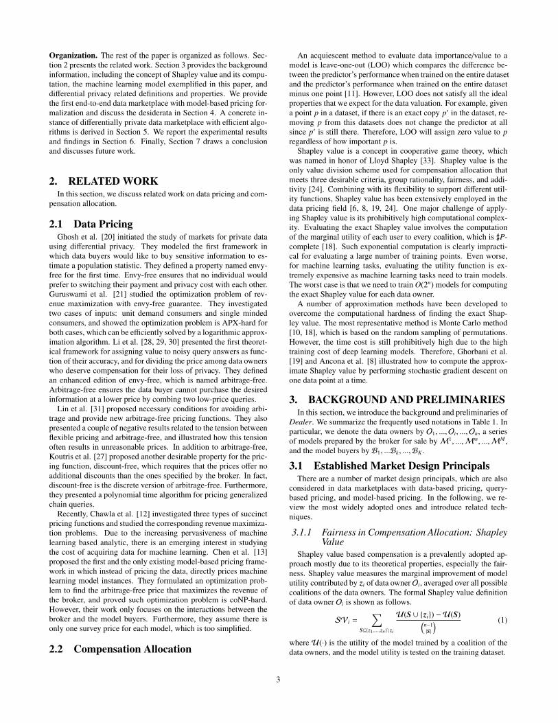
Data Owners Broker Model Buyers
… …
usage restrictions
… …
…
model
target model, budget
payment
compensation
usage restrictions
compensation
model
target model, budget
payment
…
Figure 1: An end-to-end data marketplace with model-based pric-ing framework.
Contributions. In this paper, we bridge the above gaps and addressthe identified challenges by proposing Dealer: an enD-to-end datamarketplace with model-based pricing. Dealer provides both ab-stract and general mathematical formalization for the end-to-endmarketplace dynamics (Section 4) and a specific and practical dif-ferentially private marketplace with algorithm designs that ensuresdifferential privacy of the data owners, one type of instantiation ofthe model restriction.
End-to-End Mathematical Formalization of the Marketplace. Wefirst propose an abstract mathematical formalization for Dealer withan emphasis on the understudied parts of the marketplace as dis-cussed above. An illustration is provided in Figure 1, which in-cludes three main entities and their interactions. In this generalDealer (Gen-Dealer), we define the abilities and constraints for thethree entities (i.e., data owners, broker, and model buyers). Fromthe data owners’ perspective, Gen-Dealer aims to 1) allow the dataowners to restrict their data usage by the broker; and 2) have theoption to receive extra compensation if they are willing to partiallyrelax their restrictions. From the model buyers’ perspective, Gen-Dealer provides a utility measure suitable for the model buyers’
model valuation, based on which the potential model buyers pro-vide their willingness to purchase and payment estimation. Fromthe broker’s perspective, Gen-Dealer depicts the full marketplacedynamics through abstract behavior functions. In addition to thenew features novely brought into the market design considerationby Gen-Dealer, commonly recognized market design principals arealso well-accommodated into our approach. Prominent ones in-clude: 1) compensation allocation in a fair and rational way, e.g.,based on the widely-accepted Shapley value notion; 2) arbitrage-free in model pricing, which prevents the model buyers from takingadvantage of the marketplace by combining lower-tier models soldfor cheaper prices into a higher-tier model to escape the designatedprice for that tier.
Marketplace Instantiation with Differential Privacy. We alsoprovide a concrete end-to-end differentially private data market-place instance. We focus on empirical risk minimization, a widelyused and well-studied family of supervised machine learning mod-els. For the data owners’ restrictions, we consider the privacy re-striction, which is arguably the most concerned issue for personaldata contributors. Differential privacy (DP) [16, 17], the de factostandard in privacy-preserving data analysis nowadays, is intro-duced to exemplify the data owners’ restriction requirements andwe will refer the differentially private data marketplace with model-based pricing instance by DP-Dealer. In DP-Dealer, the market-place sells a series of differentially private models to respect dataowners’ privacy restrictions. The higher tier models correspond tomodels trained on data subsets contributed by the data owners withlower DP restrictions. On the contrary, the lower tier models aretrained with higher DP restriction data subsets. We will considertwo types of data owner DP restrictions: 1) hard restriction whichhas a rigid cutting point beyond that the data owners’ data cannotbe used for training; and 2) negotiable restriction which has a nego-tiable range within that the marketplace still has the option to usethe data but with extra compensation. At the model buyers’ end,DP-Dealer addresses the challenge of mismatched model tier rank-ing standard by converting the model “manufacturing” tier rankingstandard to the model utility standard adopted by the model buyersin making purchasing decisions. DP-Dealer accommodates marketdesign principals like fair compensation allocation and arbitrage-free model pricing. To support the end-to-end marketplace dy-namics with all design considerations, DP-Dealer establishes con-strained objective functions and develops efficient algorithms to op-timize market decisions.
We briefly summarize our contributions as follows.
• A general end-to-end data marketplace with model-based pric-ing framework Gen-Dealer which is the first systematic studythat includes all market participants (i.e., data owners, broker,and model buyers). Gen-Dealer formalizes the abilities and re-strictions of the three entities and models the interactions amongthem.
• A differentially private data marketplace with model-based pric-ing DP-Dealer which instantiates the general framework. In ad-dition to incorporating market design principals, DP-Dealer pro-poses two data owner restriction schemes and provides the util-ity estimation for the model buyers to choose models best suit-ing their needs. DP-Dealer formulates a series of optimizationproblems and develops efficient algorithms to make the marketdecisions.
• A series of experiments are conducted to justify the design ofDP-Dealer and verify the efficiency and effectiveness of the pro-posed algorithms.
2
Organization. The rest of the paper is organized as follows. Sec-tion 2 presents the related work. Section 3 provides the backgroundinformation, including the concept of Shapley value and its compu-tation, the machine learning model exemplified in this paper, anddifferential privacy related definitions and properties. We providethe first end-to-end data marketplace with model-based pricing for-malization and discuss the desiderata in Section 4. A concrete in-stance of differentially private data marketplace with efficient algo-rithms is derived in Section 5. We report the experimental resultsand findings in Section 6. Finally, Section 7 draws a conclusionand discusses future work.
2. RELATED WORKIn this section, we discuss related work on data pricing and com-
pensation allocation.
2.1 Data PricingGhosh et al. [20] initiated the study of markets for private data
using differential privacy. They modeled the first framework inwhich data buyers would like to buy sensitive information to es-timate a population statistic. They defined a property named envy-free for the first time. Envy-free ensures that no individual wouldprefer to switching their payment and privacy cost with each other.Guruswami et al. [21] studied the optimization problem of rev-enue maximization with envy-free guarantee. They investigatedtwo cases of inputs: unit demand consumers and single mindedconsumers, and showed the optimization problem is APX-hard forboth cases, which can be efficiently solved by a logarithmic approx-imation algorithm. Li et al. [28, 29, 30] presented the first theoret-ical framework for assigning value to noisy query answers as func-tion of their accuracy, and for dividing the price among data ownerswho deserve compensation for their loss of privacy. They definedan enhanced edition of envy-free, which is named arbitrage-free.Arbitrage-free ensures the data buyer cannot purchase the desiredinformation at a lower price by combing two low-price queries.
Lin et al. [31] proposed necessary conditions for avoiding arbi-trage and provide new arbitrage-free pricing functions. They alsopresented a couple of negative results related to the tension betweenflexible pricing and arbitrage-free, and illustrated how this tensionoften results in unreasonable prices. In addition to arbitrage-free,Koutris et al. [27] proposed another desirable property for the pric-ing function, discount-free, which requires that the prices offer noadditional discounts than the ones specified by the broker. In fact,discount-free is the discrete version of arbitrage-free. Furthermore,they presented a polynomial time algorithm for pricing generalizedchain queries.
Recently, Chawla et al. [12] investigated three types of succinctpricing functions and studied the corresponding revenue maximiza-tion problems. Due to the increasing pervasiveness of machinelearning based analytic, there is an emerging interest in studyingthe cost of acquiring data for machine learning. Chen et al. [13]proposed the first and the only existing model-based pricing frame-work in which instead of pricing the data, directly prices machinelearning model instances. They formulated an optimization prob-lem to find the arbitrage-free price that maximizes the revenue ofthe broker, and proved such optimization problem is coNP-hard.However, their work only focuses on the interactions between thebroker and the model buyers. Furthermore, they assume there isonly one survey price for each model, which is too simplified.
2.2 Compensation Allocation
An acquiescent method to evaluate data importance/value to amodel is leave-one-out (LOO) which compares the difference be-tween the predictor’s performance when trained on the entire datasetand the predictor’s performance when trained on the entire datasetminus one point [11]. However, LOO does not satisfy all the idealproperties that we expect for the data valuation. For example, givena point p in a dataset, if there is an exact copy p′ in the dataset, re-moving p from this datasets does not change the predictor at allsince p′ is still there. Therefore, LOO will assign zero value to pregardless of how important p is.
Shapley value is a concept in cooperative game theory, whichwas named in honor of Lloyd Shapley [33]. Shapley value is theonly value division scheme used for compensation allocation thatmeets three desirable criteria, group rationality, fairness, and addi-tivity [24]. Combining with its flexibility to support different util-ity functions, Shapley value has been extensively employed in thedata pricing field [6, 8, 19, 24]. One major challenge of apply-ing Shapley value is its prohibitively high computational complex-ity. Evaluating the exact Shapley value involves the computationof the marginal utility of each user to every coalition, which is ]P-complete [18]. Such exponential computation is clearly impracti-cal for evaluating a large number of training points. Even worse,for machine learning tasks, evaluating the utility function is ex-tremely expensive as machine learning tasks need to train models.The worst case is that we need to train O(2n) models for computingthe exact Shapley value for each data owner.
A number of approximation methods have been developed toovercome the computational hardness of finding the exact Shap-ley value. The most representative method is Monte Carlo method[10, 18], which is based on the random sampling of permutations.However, the time cost is still prohibitively high due to the hightraining cost of deep learning models. Therefore, Ghorbani et al.[19] and Ancona et al. [8] illustrated how to compute the approx-imate Shapley value by performing stochastic gradient descent onone data point at a time.
3. BACKGROUND AND PRELIMINARIESIn this section, we introduce the background and preliminaries of
Dealer. We summarize the frequently used notations in Table 1. Inparticular, we denote the data owners by O1, ...,Oi, ...,On, a seriesof models prepared by the broker for sale byM1, ...,Mm, ...,MM ,and the model buyers by B1, ...Bk, ...,BK .
3.1 Established Market Design PrincipalsThere are a number of market design principals, which are also
considered in data marketplaces with data-based pricing, query-based pricing, and model-based pricing. In the following, we re-view the most widely adopted ones and introduce related tech-niques.
3.1.1 Fairness in Compensation Allocation: ShapleyValue
Shapley value based compensation is a prevalently adopted ap-proach mostly due to its theoretical properties, especially the fair-ness. Shapley value measures the marginal improvement of modelutility contributed by zi of data ownerOi, averaged over all possiblecoalitions of the data owners. The formal Shapley value definitionof data owner Oi is shown as follows.
SVi =∑
S⊆z1 ,...,zn\zi
U(S ∪ zi) −U(S)(n−1|S|
) (1)
where U(·) is the utility of the model trained by a coalition of thedata owners, and the model utility is tested on the training dataset.
3
Table 1: The summary of notations.Notation DefinitionOi the ith data ownerMm the mth modelBk the kth model buyer
Ztrain = z1, z2, ..., zn training datasetXtrain = x1, x2, ..., xn features of training datasetytrain = y1, y2, ..., yn labels of training dataset
zi = xi, yi the ith training dataZtest testing datasetXtest features of testing datasetytest labels of testing datasetU model utilitySV Shapley valueUV utility valuationUF utility functionMR model risk factorMB manufacturing budgetDR data owner restriction functionε, δ parameters for the DPbc base compensationec extra compensationtm target model
〈p(ε1), p(ε2), ..., p(εM)〉 optimal pricing(m, spm[ j]) survey price point(m, pm[ j]) complete price point
Monte Carlo Simulation Method. Since the exact Shapley valuecomputation is based on enumeration which is prohibitively expen-sive, we adopt a commonly used Monte Carlo simulation method[10, 18] to compute the approximate Shapley value. We first sam-ple random permutations of the data points corresponding to dif-ferent data owners, and then scan the permutation from the firstelement to the last element and calculate the marginal contributionof every new data point. Repeating the same procedure over mul-tiple Monte Carlo permutations, the final estimation of the Shapleyvalue is simply the average of all the calculated marginal contri-butions. This Monte Carlo sampling gives an unbiased estimateof the Shapley value. In practical applications, we generate MonteCarlo estimates until the average has empirically converged and theexperiments show that the estimates converge very quickly. There-fore, Monte Carlo simulation method can control the degree of ap-proximation, i.e., the more permutations, the better the accuracy .The detailed algorithm is shown in Algorithm 1, where |π| is thenumber of permutations. The larger the |π|, the more accurate thecomputed Shapley value.
Algorithm 1: Monte Carlo Shapley value computation.input : Ztrain = (Xtrain, ytrain) and Ztest = (Xtest, ytest).output: Shapley value SVi for each data zi in Ztrain.
1 initialize SVi = 0;2 for k=1 to |π| do3 we have a training dataset ordered in πk,
Zktrain = zπk
1, zπk
2, ..., zπk
n;
4 for i=1 to n do5 SV(zπk
i) = U(zπk
1, ..., zπk
i) −U(zπk
1, ..., zπk
i−1);
6 SVπki
= SVπki
+ SV(zπki);
3.1.2 VersioningFor a perfect world, the broker would sell a personalized model
to each model buyer at a different price to maximize the revenue.
However, such personalized pricing is rarely possible in practicalapplications. On the one hand, it is expensive to train differentmodels for different model buyers. On the other hand, it is difficultto set an array of prices for the same model. Even if we could, itwould be impossible to get model buyers to stay within their in-tended pricing strata rather than to look for the lowest price. Fi-nally, the broker runs the risk of annoying or even alienating modelbuyers if they charge different prices for the same model.
There is a practical way to set different prices for the same train-ing dataset without incurring high costs or offending model buyers.We can do it by offering the training dataset in different versions de-signed to attract different types of model buyers. With this strategy,which is called versioning [32], model buyers segment themselves.The model version they choose reveals the value they place on thetraining dataset and the price they are willing to pay. Therefore, inour model marketplace, the broker would train M different modelversions by injecting different noise to different subsets of trainingdata contributed by the data owners.
3.1.3 Arbitrage-free in Model PricingArbitrage is possible when the “better” model can be obtained
more cheaply than the advertised price by combining two or moreworse models with lower price. Arbitrage complicates the inter-actions between the broker and the model buyers, i.e., the modelbuyers need to carefully choose the models to achieve the lowestprice, while the broker may not achieve the revenue intended byher advertised prices. Therefore, an arbitrage-free pricing functionis highly desirable. We say a pricing function is arbitrage-free if itsatisfies the following two properties proved in [13, 30].
Property 1. (Monotonicity). Given a function f : (R+)k → R+,we say f is monotone if and only if for any two vectors x, y ∈ (R+)k,x ≤ y, we have f (x) ≤ f (y).
Property 2. (Subadditivity). Given a function f : (R+)k → R+,we say f is subadditive if and only if for any two vectors x, y ∈(R+)k, we have f (x + y) ≤ f (x) + f (y).
3.2 Machine Learning ModelsIn this paper, we focus on the Empirical Risk Minimization (ERM),
which is a widely-applied tool in machine learning. Denote thetraining dataset by Ztrain := zi, i = 1, 2, ..., n, where zi ∼ D andzi = (xi, yi). The xi ∈ R
d is the d-dimensional feature vector andyi is the response value which can be −1,+1 for binary classifica-tion task or [0, 1] for regression task. The ERM has the followingobjective function:
arg minw∈Ω
L(w; Ztrain) + λ‖w‖22 = arg minw∈Ω
n∑i=1
1n
l(w; zi) + λ‖w‖22, (2)
where L(w; Ztrain) =∑n
i=1 l(w; zi) is the empirical loss averagedfrom losses taken from all zi, λ‖w‖22 is the regularizer and Ω is theconstraint set. In this paper, we focus on models with convex, Lip-schitz continuous, and smooth loss (with respect to w) functions.The formal definitions are in the following.
Definition 1. (Convex Loss Function) A loss function l(w) :Rd → R is called convex if for all w1,w2 ∈ R
d,
|l(w1) − l(w)2| ≥ 〈∇l(w2),w1 − w2〉. (3)
In addition, if l(w1) − l(w)2 ≥ 〈∇l(w2),w1 − w2〉 +µ
2 ‖w1 − w2‖22, for
µ > 0, l(w) is µ-strongly convex.
4
Definition 2. (Lipschitz continuous Loss Function) A loss func-tion l(w) : Rd → R is called L-Lipschitz continuous if for allw1,w2 ∈ R
d,
|l(w1) − l(w)2| ≤ L‖w1 − w2‖2. (4)
Definition 3. (Smooth Loss Function) A loss function l(w) :Rd → R is called β-smooth if for all w1,w2 ∈ R
d,
l(w1) − l(w)2 ≤ 〈∇l(w2),w1 − w2〉 +β
2‖w1 − w2‖
22 (5)
We focus on the loss functions satisfying the above assumptionslike least square loss, logistic loss, and smoothed hinge loss. Inmachine learning, these losses are thoroughly studied with theo-retical properties like generalization performance, and easy to usewith efficient optimization algorithm with guaranteed convergence.Furthermore, their differentially private versions are also equippedwith efficiency, utility, and privacy guarantees. As a result, we fo-cus on this particular type of machine learning models in our mar-ket design for a thorough understanding of our proposed market.However, we would like to mention that most of our algorithmscan be applied to other types of machine learning models like thepopular deep learning family.
3.3 Differential PrivacyDifferential privacy is a formal mathematical tool for rigorously
providing privacy protection. However, none of the existing (pub-lished) data marketplace with model-based pricing paper has con-sidered it and it is still unknown how it can be incorporated in datamarketplace with model-based pricing and how it affects marketdesigns when adopted.
Definition 4. (Differential Privacy) A randomized algorithmAis (ε, δ)-differentially private, if for any pair of datasets S and S′that differs in one data sample, and for all possible output O ofA,the following holds,
P[A(S) ∈ O] ≤ eεP[A(S′) ∈ O] + δ, (6)
where the probability is taken over the randomness ofA.
In practice, for a meaningful DP guarantee, the parameters are cho-sen as 0 < ε ≤ 1, δ 1
N , where N is the number of data samples.
Lemma 1. (Simple Composition) LetA j be an (ε j, δ j)-differentiallyprivate algorithm. We have A = (A1, ...,AJ) is (
∑Jj=1 ε j,
∑Jj=1 δ)-
differentially private.
Lemma 1 is essential for DP mechanism design and analysis, whichenables algorithm designers to compose elementary DP operationsinto a more sophisticated one. More importantly, we will showthat it plays a crucial role in model market design as well. That is,Lemma 1 determines that DP is an appropriate mechanism for ver-sioning models, based on which prices have to satisfy the arbitrage-free property.
Definition 5. (`2-sensitivity) A function f : DN → Rd has `2
sensitivity ∆2 if
maxneighboring S,S′
‖ f (S) − f (S′)‖2 = ∆2 (7)
For training ERM with DP restriction, a popular method is the ob-jective perturbation, which perturbates the objective function of themodel with quantified noise. Conventional objective perturbationonly supports DP guarantee for the exact optimum, which is hardly
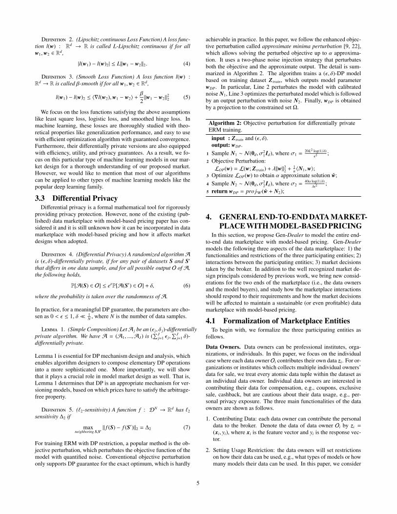
achievable in practice. In this paper, we follow the enhanced objec-tive perturbation called approximate minima perturbation [9, 22],which allows solving the perturbed objective up to α approxima-tion. It uses a two-phase noise injection strategy that perturbatesboth the objective and the approximate output. The detail is sum-marized in Algorithm 2. The algorithm trains a (ε, δ)-DP modelbased on training dataset Ztrain, which outputs model parameterwDP. In particular, Line 2 perturbates the model with calibratednoise N1, Line 3 optimizes the perturbated model which is followedby an output perturbation with noise N2. Finally, wDP is obtainedby a projection to the constrained set Ω.
Algorithm 2: Objective perturbation for differentially privateERM training.
input : Ztrain and (ε, δ).output: wDP.
1 Sample N1 ∼ N(0d, σ21 Id), where σ1 =
20L2 log(1/δ)ε2 ;
2 Objective Perturbation:LOP(w) = L(w; Ztrain) + λ‖w‖22 + 1
n 〈N1,w〉;3 Optimize LOP(w) to obtain α approximate solution w;4 Sample N2 ∼ N(0d, σ
22 Id), where σ2 =
40α log(1/δ)λε2 ;
5 return wDP = pro jW(w + N2);
4. GENERAL END-TO-END DATA MARKET-PLACE WITH MODEL-BASED PRICING
In this section, we propose Gen-Dealer to model the entire end-to-end data marketplace with model-based pricing. Gen-Dealermodels the following three aspects of the data marketplace: 1) thefunctionalities and restrictions of the three participating entities; 2)interactions between the participating entities; 3) market decisionstaken by the broker. In addition to the well recognized market de-sign principals considered by previous work, we bring new consid-erations for the two ends of the marketplace (i.e., the data ownersand the model buyers), and study how the marketplace interactionsshould respond to their requirements and how the market decisionswill be affected to maintain a sustainable (or even profitable) datamarketplace with model-based pricing.
4.1 Formalization of Marketplace EntitiesTo begin with, we formalize the three participating entities as
follows.
Data Owners. Data owners can be professional institutes, orga-nizations, or individuals. In this paper, we focus on the individualcase where each data ownerOi contributes their own data zi. For or-ganizations or institutes which collects multiple individual owners’data for sale, we treat every atomic data tuple within the dataset asan individual data owner. Individual data owners are interested incontributing their data for compensation, e.g., coupons, exclusivesale, cashback, but are cautious about their data usage, e.g., per-sonal privacy exposure. The three main functionalities of the dataowners are shown as follows.
1. Contributing Data: each data owner can contribute the personaldata to the broker. Denote the data of data owner Oi by zi =
(xi, yi), where xi is the feature vector and yi is the response vec-tor.
2. Setting Usage Restriction: the data owners will set restrictionson how their data can be used, e.g., what types of models or howmany models their data can be used. In this paper, we consider
5
a natural strategy, where Oi sets one restriction per each modelto train. That is, for model Mm, Oi provides Data Restrictionfunction DRm
i . Two types of restriction functions are modeledin this paper. The first is the simpler “in or out” restriction,where DRm
i = 0, 1 is an indication function providing hardrestriction on whether zi is allowed to be used for training themth model (DRm
i = 1) or not (DRmi = 0). The second provides
negotiable ranges that DRmi is not only a function of the model
tier but also related to extra compensation (ecmi ): DRm
i (ecmi ) =
0, 1. That is, zi can be used for training modelMm if the extracompensation ecm
i satisfies Oi’s expectation.
3. Receiving Compensation: After the sales, the data owners re-ceive compensation based on their data usage. In addition, extracompensation will be paid if their data is used after negotiation.In particular, the extra compensation ecm
i is a function of riskfactor riskm to be introduced in the next subsection: ecm
i = 0, ifriskm
i ≤ MRm and is an nondecreasing nonnegative function of
riskmi −MR
m if riskmi >MRm.
Discussion 1. Compared to existing machine learning modelmarketplace designs which limit the data owners actions to merelycontribute data and receive compensation, our formulation has thefollowing two strengths: 1) it allows the data owners to set data us-age restrictions; 2) the negotiable-type restrictions help data ownerto better estimate the value of their personal data, which is oftendifficult for individuals who have limited market information andevaluation of data usage risk. We believe that by better model-ing the data owner by providing the rights on setting data usagerestrictions and receiving extra compensation, it will eventually in-centivize more data owners to contribute their data.
Assumption 1. The data owners do not fake data. Each dataowner only contributes one data sample and all data are indepen-dent.
Remark 1. In practice, each data owner may have multiple atomicdata tuples, and those data tuples among different data owners maybe correlated. Therefore, we need to consider their relationshipwhen we allocate compensation. For the correlated data, we leaveit as an open question.
Model Buyers. Model buyers can be industries or everyday users,who are interested in purchasing machine learning models to ei-ther integrate into their product or support certain decision making.They have very different budgets and model utility requirements. Inthis paper, we focus on the single minded model buyers who willpurchase at most one model. There are two functionalities of themodel buyers as follows.
1. Providing Purchase Willingness: Bk provides the purchase will-ingness by providing (tmk, vk), where the target model tmk ∈
1, ...,M indicates target model of Bk and vk is the purchas-ing budget. We note that the number of potential model buyerscan be very large, but the purchase willingness of hundreds ofsampled model buyers is enough for the broker to make marketdecision.
2. Model Transaction: Bk decides to purchase the target model ornot by comparing the released price p(tmk) by the broker andher budget.
Broker. The broker collects data from the data owners and trainsa series of machine learning models for sale to the model buyers.
Let the Models be M1, ...,Mm, ...,MM . As discussed, a commonversioning strategy is to sell the models in various tiers, from thelowest tier (sayM1) to the highest tier (sayMM). For these mod-els, it sets prices 〈p(M1), ..., p(MM)〉. In addition, we assume thebroker is honest in the sense that it will strictly follow contractwith the data owners, e.g., respecting their usage restrictions, al-locating the compensation based on the true data usage. The bro-ker also wishes to remain competitive by training the best modelfor each tier within that tier’s resource budget. More importantly,the broker interacts with both the data owners and the model buy-ers, and makes various market decisions, which are detailed inthe later sections. Finally, we assume there is a model risk fac-tor MRm associated with each model Mm to be detailed in Sec-tion 4.3. The model risk measures how large certain risk is tothe data owner who participates in the model training. When therisk is low, the broker usually puts high restrictions on data us-age, which often leads to limited data information extraction. As aresult, the lower risk model often corresponds to lower tier mod-els coming with a lower price. We denote such connection by〈p(MR1), ..., p(MRM)〉, where MR1
≤ ... ≤ MRM and the pricesatisfies arbitrage-free with respect to the model risk. In a moregeneralized market setting, multiple brokers can co-exist, whichforms a competitive relationship. To focus on the principal func-tionalities of a broker, we follow existing work [6, 13, 24] to con-sider only a single broker case in this paper.
4.2 Formalization of Marketplace DynamicsIn this subsection, we formalize the data marketplace dynamics,
which consist of the interaction between the data owner and thebroker, the interaction between the model buyer and the broker.
Interaction between Data Owner and Broker.
• Data Collection: The broker posts model tiers M1, ...,MM andexplains each tier’s model riskMRm to the data owners and howeach tier will possibly be compensated if a data owner choosesto participate. The data owner Oi contributes data zi and set datausage restriction DRm
i as well as a potential extra compensationecm
i if he is willing to negotiate, for all m = 1, ...,M. Recall thatDR
mi and ecm
i are functions ofMRm.
• Compensation Allocation: After training the models under datausage restrictions (see Model Training part in the next subsec-tion), the broker pays compensation to the data owners accord-ing to the Compensation Allocation market decision algorithmdetailed in the next subsection. Three key quantities are UtilityValuation to modelMm: UVm
i , its base compensation: bcmi , and
extra compensation: ecmi .
Interaction between Model Buyer and Broker.
• Market Survey: The broker posts the models tiers M1, ...,MM
to the potential model buyers. Each model buyer Bk providespurchase willingness (tmk, vk).
• Model Transaction: The broker makes the model pricing 〈p1, ..., pM〉
(see Model Pricing in the next subsection) based on (tmk, vk).The model buyers then make purchase decisions and completethe transaction if meeting budget restriction.
Discussion 2. The data owners’ contributing willingness is basedon risk level if their data is used for training modelMm, while themodel buyers’ purchasing willingness is based on the usefulnessof the model (i.e., model utility). Thus, the two ends have a dif-ferent standard for the same model tier, which requests the brokerto make optimal market decisions to bridge the two ends’ differentrequirements.
6
4.3 Marketplace Decision Making
4.3.1 Model Training under Data Usage RestrictionIn this part, we propose a brand new versioning strategy, which
centers on the data owners’ perspective, rather than simply low-ering the quality of the model which merely considers the modelbuyers’ payment ability like [13].
Versioning. In general, more data owners’ contribution makesthe “manufacturing cost” of the corresponding model cheaper, be-cause the broker has many alternative choices and tends to dom-inate the compensation bargain. On the contrary, for the modelswith higher risk, much fewer data owners are willing to participate,which makes the broker have to pay higher compensation to in-trigue more data contribution. With increased manufacturing cost,the product (i.e., the model for sale) price should increase. Thus,we propose to set a version based on the participating risk, which isout of the data owners’ perspective. However, since the model buy-ers, in general, do not care about the risk factor but the model utility,the broker should provide conversion from the risk-tiering standardto the model utility standard for each model tier. To bridge bothends, the broker needs to make market decisions (e.g., set modelpricing) constrained by all participating entities’ requirements asconstraints. As a result, it assures our claim that designing the datamarketplace with model-based pricing from end to end is of neces-sity and importance.
Recall that each modelMm is associated with model riskMRm.The versioning is a process where the broker trains a series of mod-els with different model risks:MR1, ...,MRM under the restrictionsof all n data owners DRm
i and extra compensation requirementsecm
i . On the model buyer’s end, the broker in our marketplace willprovide a utility function UF (MRm) for each risk-based modeltier, since the utility is the fundamental model property interestedto the model buyers.
In comparison, the versioning strategy of the existing model mar-ket [13] produces different versions of models by controlling modelutility through directly adding noise to the model parameters, in or-der to suit different model buyers coming with various paymentability. Obviously, their simplified versioning strategy fails to re-flect the true “model manufacturing cost”.
Model Utility Maximization with Manufacturing Budget. GivenOi = (zi,DR
mi ) orOi = (zi,DR
mi (ecm
i )), for i = 1, 2, ..., n, the brokertrains each modelMm under data usage restrictions and tries its bestto train the best model for each model tier to remain competitive.Let data owner Oi’s preferred model risk be riski, which indicatesthe highest risk she wants to take (without extra compensation). Inthis paper, we instantiate the data restriction DRm
i function as fol-lows: 1) for the hard restriction case, DRm
i = I(MRm≤ riski),
i.e., the data can be used forMm only when the model riskMRm
is lower than the data owner’s preferred risk riski; 2) for the nego-tiable case, DRm
i (ecmi ) = I(MRm
≤ riski) ∧ I(ecmi ), i.e., the data
can be used either the model risk is lower than the preferred risk,or the extra compensation is made.
For the simpler hard data usage restriction, the broker trainsmodel Mm with data Subset: Sm : i ∈ 1, 2, ..., n, s.t. DRm
i = 1.For the negotiable data usage restriction, under limited manufac-turing budget MB, the broker needs to decide whose data worththe extra compensation, so that the utility valuation of the trainedmodel will be maximized for the broker to be competitive in themarket. Denote the utility valuation (to be detailed in the next sub-section) of zi to model Mm by UVm
i . We formalize the subsetselection of Sm as a training budget constrained utility valuation
maximization problem as follows.
arg maxSm⊆z1 ,...,zn
∑i∈Sm
UVmi , (8)
s.t. (∑i∈Sm
(bcmi + ecm
i (max0,MRm− riski))) ≤ MBm. (9)
In the above, the utility value UVmi and the base compensation
bcmi should satisfy certain market design principals, which will be
discussed in the following.
4.3.2 Compensation AllocationIn this part, we elaborate how Gen-Dealer allocates base com-
pensation bcmi and utility valuation UVm
i strategy. Recall that formodel Mm, its base compensation bcm
i and extra compensationecm
i . The extra compensation is a function of the data owner pre-ferred risk riski and the model risk MRm: if MRm
≤ riski, dataowner Oi will participate the training ofMm with only base com-pensation; else if MRm > riski, ecm
i is charged with respect toMR
m− riski, i.e., the broker needs to pay for the extra risk the data
owner suffers. Together, ecmi is a function of max0,MRm
− riski
as shown in Equation (9).For the base compensation, Gen-Dealer allocates it based on the
zi’s Utility ValueUVmi , whereUVm
i is based on the (approximate)Shapely value and divides bcm
i according to the relative Shapelyvalue. This way, the true contribution of data owner Oi to modelMm can be evaluated and the base compensation is consistent withmarket design principals. To be practical, efficient approximationalgorithms will be utilized.
To summarize, Gen-Dealer will allocate the compensation todata ownerOi for participating modelMm as bcm
i +ecmi (max0,MRm
−
riski)). The total compensation allocated to data owner Oi is:
M∑m=1
I(i ∈ Sm) ·[bcm
i + ecmi (max0,MRm
− riski))], (10)
where I(i ∈ Sm) is an indicator function for indication whether zi isin data subset Sm for trainingMm.
4.3.3 Market Survey and Revenue MaximizationIn this part, we show how to construct the market survey between
the broker and the potential model buyers, and how the broker max-imizes the revenue based on the market survey.
Market Survey. Prior to release models and prices for sale, thebroker will estimate the price for each model through a market sur-vey, which can be done by the broker himself or by third-partycompanies like consultation service providers. Let the survey sizeby K′, i.e., K′ potential model buyers are recruited to provide theirpurchasing willingness. The survey result will contain K′ tuples,one from each survey participant. For the kth survey participant, itprovides (tmk, vk), where tmk ∈ 1, ...,M is the target model andvk is the acceptable price of model tmk she is willing to purchase.We note that the survey participants may have an incentive to reportlower valuations in order to decrease the price, which can be alle-viated by the digital goods auction [7] based on two approaches:random-sampling mechanisms and consensus estimates.
Revenue Maximization (Model Pricing).With the surveyed purchasing willingness, the broker will price
each model in the aim of maximizing revenue and at the same time
7
following the market design principal of arbitrage-free. To do so,the revenue maximization problem is formulated as follows.
arg max〈p(MR1),...,p(MRM )〉
M∑m=1
K′∑k=1
p(MRm) · I(tmk == m) · I(p(MRm) ≤ vk),
(11)
s.t. p(MRm) + p(MRm′ ) ≥ p(MRm +MRm′ ), MRm,MRm′≥ 0,(12)
p(MRm) ≥ p(MRm′ ), MRm≥ MR
m′≥ 0, (13)
p(MRm) ≥ 0, MRm≥ 0, (14)
whereMRm is the model risk defined in Section 4.1, p(MRm) is themodel price for modelMm whose model risk isMRm. In the nextsection, we will see that this problem is co-NP hard and we willprovide an efficient approximation with accuracy bound algorithmthere for our DP-Dealer instance.
5. A DIFFERENTIALLY PRIVATE DATA MAR-KETPLACE INSTANCE AND EFFICIENTAPPROXIMATE OPTIMIZATION
In this section, we propose a concrete realization of Gen-Dealer,a differentially private data marketplace with model-based pricingframework DP-Dealer. We illustrate the functionalities and restric-tions of the data owners and the model buyers in DP-Dealer inSections 5.1 and 5.2, respectively. Furthermore, in Section 5.3, wepresent the broker’s functioning in DP-Dealer by providing con-crete solutions, which are efficient approximate optimization al-gorithm to make the market practical. Finally, we summarize thecomplete DP-Dealer dynamics in Section 5.4.
5.1 Data OwnerWe provide a data owner instance by instantiating its risk factor,
data restrictions, and extra compensation functions. For the riskfactor, we focus on the privacy-preserving issue, which is arguablyone of the major concerns limiting individual users from contribut-ing their data. The data owners wish to contribute data for modeltraining with a certain level of privacy in exchange of a fair share ofcompensation. We follow the differential privacy notion and instan-tiate both the hard and negotiable data usage restriction cases. Letthe model risk factorMRm of modelMm be described by εm whichcorresponds to εm-differential privacy of the model. Traditional DPsystem and algorithm designs mostly consider the differential pri-vacy strictness out of the broker’ and the model buyers’ perspec-tive, which sets it as a tradeoff factor as long as it affects the modelutility within a certain level. This overlooks the true privacy de-mand of the data owners. For those who do consider personalizedDP budget, they seldom consider what value the privacy parameteractually means to the data owner. Under such a lack of reward sce-nario, the data owner still has difficulty evaluating their own privacydemands. Our design allows the data owners to choose their ownprivacy preference and receives rewards for providing more usefulpersonal information. We believe it is a good starting point for apractical data marketplace with model-based pricing that respectsthe data owners’ privacy demand and incentivizes the data ownersfor their personal data contribution.
Under the differential privacy risk factor, the three functionalitiesof data owner Oi are shown as follows.
1. Contributing Data: data ownerOi contributes her data zi = (xi, yi)to the broker;
2. Setting Usage Restriction: let the personal risk preference riski
be (εi, δ)-DP1.
Hard DP requirement. In the first simplified case, each dataowner Oi chooses whether her data is allowed for training modelMm with certain level of privacy restriction by DP parameterε
pre f eri . That is, data owner Oi only allows her data to be used
for models with DP restrictions stricter than εi, i.e., εm ≤ εi.Then, the data restrictionDRm
i = I(εm ≤ εi).
Negotiable DP requirement. We further consider a more com-plicated data owner strategy, where the data owners have moreoptions for making their own trade-offs between compensationand privacy risk. For data owner Oi, in addition to DP require-ment εi, she is also willing to trade some of the privacy for morecompensation. To do so, we introduce an extra compensationfunction ecm
i (εi, εm), which pays an extra fraction of the base
compensation (allocated based on Shapley value) to compen-sate for the higher privacy risk. In this case, the data usagerestriction function is also a function of the extra compensa-tion: I(ecm
i (εi, εm)) which indicates whether the extra compen-
sation has been allocated. Thus, DRmi (ecm
i ) = [I(εm ≤ εi) ∧I(ecm
i (εi, εm))].
3. Receiving Compensation: For both cases, we let the base com-pensation bcm
i to be proportional to the relative approximatedShapley value (see the broker instance in the following). In ad-dition, for the negotiable case, we introduce the extra compen-sation function if εm > εi but the broker is willing to use zi fortraining Mm to maximize the model value (subject to the con-straint of the manufacturing budget).
Extra Compensation Function. In particular, we present threetypes of the extra compensation function ecm
i (εi, εm): concave,
linear, and convex, to model three user inclinations of their per-sonal privacy risks: reserved, balanced, and casual, correspond-ingly.
• linear: ecmi (εi, ε
m) = ρmi bcm
i max0, εm − εi;
• convex: ecmi (εi, ε
m) = ρmi bcm
i (max0, εm − εi)2;
• concave: ecmi (εi, ε
m) = ρmi bcm
i (max0, εm − εi)12 ;
For the ease of presentation, we use ecmi to replace ecm
i (εi, εm) to
express the extra compensation of data owner Oi on modelMm inthe following.
Discussion 3. For all cases, each data owner Oi has the max-imum total potential privacy leakage
∑Mm=1 ε
mi . In this work, we
assume the data owners do not have too much information aboutthe data marketplace except the information given by the broker.Thus, they invariably invest their total privacy budget to each ofthe M models, which can be suboptimal for certain owners. In thefuture, we will consider more informed data owners, who have notonly more knowledge about the data marketplace, e.g., the demandfor each type of model, but also the quality and privacy restrictionsof other data owners. With the additional market information, dataowners can allocate their total privacy leakage more intelligentlyby investing their privacy budget towards models returning themmore compensation.
1In this paper, we assume the δ is sufficiently small so that wedo not consider its value and composition for the remaining of thepaper for convenience.
8
Assumption 2. The goal of adding DP noise in models is tolimit what can be inferred from the models about individual train-ing data tuples. Therefore, it is better for the broker to supportthe relationship between DP parameter ε and what can be inferredfrom the models to the data owners. We note that such a relation-ship can be implemented by [23].
5.2 Model BuyerThe model buyers in DP-Dealer have the same functionalities
with the model buyers in Gen-Dealer shown in Section 4.1 whenconsidering the differential privacy instantiation.
Assumption 3. The arbitrage-free property of the models is es-tablished in terms of the differential privacy budget.
Remark 2. In practice, the model buyers can buy a couple ofweak models and convert those weak models to strong ones by em-ploying some machine learning techniques such as ensemble learn-ing, bagging and boosting. However, it may be infeasible to for-mally characterize how model combinations behave in terms of themodel utility. Therefore, instead of ensuring the models to satisfyarbitrage-free in terms of model utility, we ensure that the modelssatisfy arbitrage-free in terms of DP parameter.
5.3 BrokerIn this part, we present the broker’s functioning in the differ-
entially private data marketplace by providing concrete solutionsfor selecting optimal training subsets with budget constraints, themarket survey to potential model buyers, and pricing models forrevenue maximization with an arbitrage-free guarantee.
5.3.1 Selecting Optimal Training Subsets with Bud-get Constraint
Given the training data along with the data owners’ privacy andextra compensation functions, the broker aims to train the highestvalued model for each price tier with the constraint on the privacyand manufacturing/compensation budget. According to differentdata owners’ requirements, the broker has two types of workflows.
Processing the Hard DP Restriction. In this case, for model tierεm, the broker is allowed to release modelMm trained strictly witha subset Sm within the data owners Oi, where εi ≤ ε
m. We formalizethe optimization problem as follows.
arg maxSm
∑i∈Sm
SVmi , s.t.
∑i∈Sm
bcmi ≤ MB
m (15)
We omit the solutions for Equation (15) because it is a special caseof the following Equation (16).
Processing the Negotiable DP Restriction. A more practical caseis the negotiable DP restriction, where the broker has the optionto decide whether to intrigue high quality data owners to lowertheir privacy restriction with extra compensation. We formalizeit as the following Budget Constrained Maximum Value Problem(BCMVP) on modelMm:
arg maxSm
∑i∈Sm
SVmi , s.t.
∑i∈Sm
(bcmi + ecm
i ) ≤ MBm (16)
whereMBm is the manufacturing budget of modelMm. In essence,we reallocate the payment of lower valued data owners to becomethe extra compensation of higher valued data owners.
The above problem is difficult to be exactly solved. In fact,we prove the problem is NP-hard. Given this NP-hard complex-ity, we then present three approximation algorithms. First, we
present a pseudo-polynomial time algorithm using dynamic pro-gramming technique. Then, we present a fully polynomial-time ap-proximation scheme with the worst case bound if each data owner’scompensation is not too large. Finally, we propose an enumera-tion guess based polynomial time approximation algorithm with theworst case bound by relaxing the compensation constraint, whichuses the pseudo-polynomial time algorithm as a subroutine.
NP-hardness proof. We prove that BCMVP is NP-hard by show-ing that the well-known partition problem is polynomial time re-ducible to BCMVP.
Definition 6. (Decision Version of BCMVP) Given a set S of ndata owners with their corresponding privacy compensation bcm
1 +
ecm1 , bcm
2 +ecm2 , ..., bcm
n +ecmn and Shapley valueSVm
1 ,SVm2 , ...,SV
mn ,
the decision version of BCMVP has the task of deciding whetherthere is a subset S1 ⊆ S such that
∑i∈S1
bcmi + ecm
i ≤ B and∑i∈S1SV
mi ≥ V.
Definition 7. (Decision Version of Partition Problem) Given aset S of n positive integer values v1, v2, ..., vn, the decision versionof partition problem has the task of deciding whether the given setS can be partitioned into two subsets S1 and S2 such that the sumof the integers in S1 equals the sum of the integers in S2.
Theorem 1. The decision version of BCMVP is an NP-hard prob-lem.
Proof. We show that there exists a polynomial reduction by prov-ing that there exists a subset S1 ⊆ S such that
∑i∈S1
bcmi + ecm
i ≤ Band
∑i∈S1SV
mi ≥ V if and only if there is a partition S1 and S2 such
that the sum of the integer values in S1 equals the sum of the inte-ger values in S2. We construct the polynomial reduction as follows.Consider the following instance of BCMVP: bcm
i + ecmi = vi and
SVmi = vi for i = 1, 2, ..., n, and B = V = 1
2
∑ni=1 vi.
We show the reduction as follows.(1) If there exists a partition S1 and S2 such that the sum of the
integer values in S1 equals to the sum of the integers in S2, thereexists S1 and S2 such that
∑i∈S1
vi =∑
i∈S2vi = 1
2
∑ni=1 vi. We choose
the set of data owners S1 in BCMVP and we have∑
i∈S1bcm
i +ecmi =∑
i∈S1vi = 1
2
∑ni=1 vi = B and
∑i∈S1SV
mi =
∑i∈S1
vi = 12
∑ni=1 vi = V .
Therefore, we know that there exists a subset S1 ⊆ S such that∑i∈S1
bcmi + ecm
i ≤ B and∑
i∈S1SV
mi ≥ V .
(2) If there exists a subset S1 ⊆ S such that∑
i∈S1bcm
i + ecmi ≤
B and∑
i∈S1SV
mi ≥ V , we partition the set S into S1 and S2 =
S − S1. We have∑
i∈S1bcm
i + ecmi =
∑i∈S1
vi ≤ B = 12
∑ni=1 vi and∑
i∈S1SV
mi =
∑i∈S1
vi ≥ V = 12
∑ni=1 vi. This implies that
∑i∈S1
vi =12
∑ni=1 vi. We also have
∑i∈S2
vi =∑n
i=1 vi −12
∑ni=1 vi = 1
2
∑ni=1 vi.
Therefore, there exists a partition S1 and S2 such that∑
i∈S1vi =∑
i∈S2vi = 1
2
∑ni=1 vi.
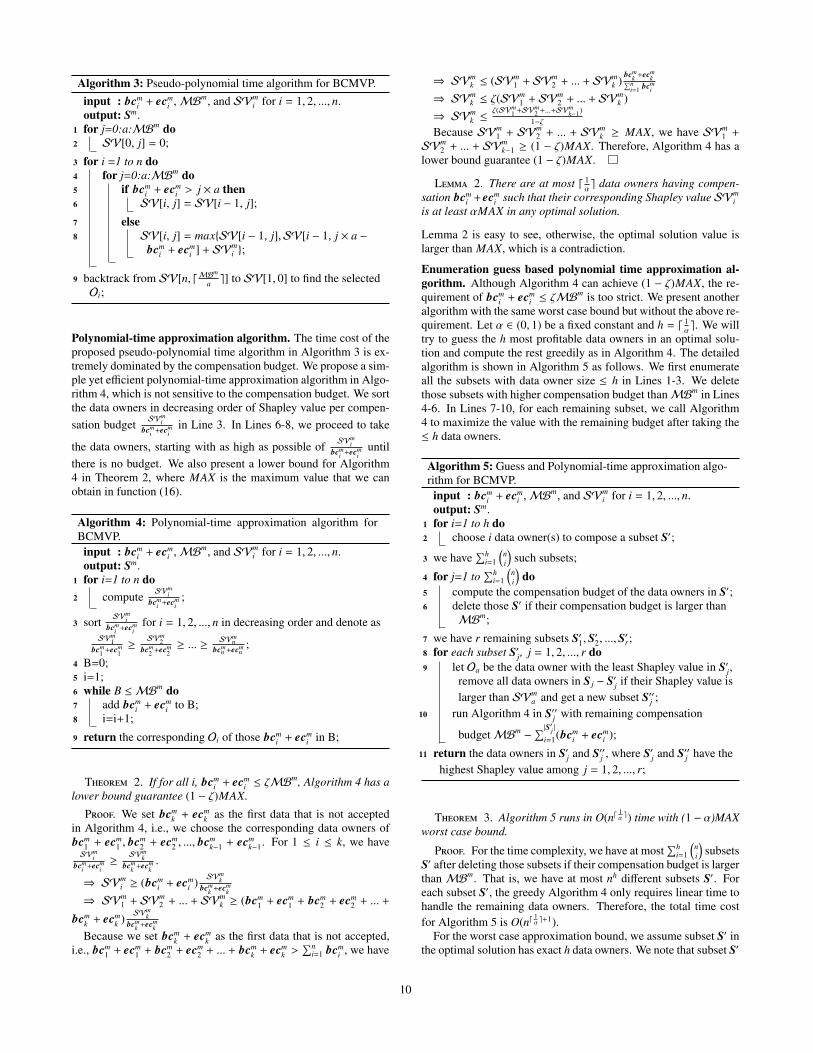
Pseudo-polynomial time algorithm. We present a pseudo-polynomialtime algorithm for BCMVP. Pseudo-polynomial means that ouralgorithm has the polynomial time complexity in terms of MBm
rather than the number of data owners n. We divide MBm intodMB
m
a e parts, where a is the greatest common divisor in bcmi + ecm
ifor all i = 1, 2, ..., n. We define SV[i, j] as the maximum BCMVPthat can be attained with compensation budget ≤ j × a by onlyusing the first i data owners. The detailed algorithm is shown inAlgorithm 3. In Line 5, if the compensation budget is not enough,we do not need to consider the ith data owner. Otherwise, we cantake Oi if we can get more value by replacing some data ownersfrom O1, ...,Oi−1 in Line 8.
9
Algorithm 3: Pseudo-polynomial time algorithm for BCMVP.input : bcm
i + ecmi ,MBm, and SVm
i for i = 1, 2, ..., n.output: Sm.
1 for j=0:a:MBm do2 SV[0, j] = 0;
3 for i =1 to n do4 for j=0:a:MBm do5 if bcm
i + ecmi > j × a then
6 SV[i, j] = SV[i − 1, j];
7 else8 SV[i, j] = maxSV[i − 1, j],SV[i − 1, j × a −
bcmi + ecm
i ] + SVmi ;
9 backtrack from SV[n, dMBm
a e] to SV[1, 0] to find the selectedOi;
Polynomial-time approximation algorithm. The time cost of theproposed pseudo-polynomial time algorithm in Algorithm 3 is ex-tremely dominated by the compensation budget. We propose a sim-ple yet efficient polynomial-time approximation algorithm in Algo-rithm 4, which is not sensitive to the compensation budget. We sortthe data owners in decreasing order of Shapley value per compen-sation budget
SVmi
bcmi +ecm
iin Line 3. In Lines 6-8, we proceed to take
the data owners, starting with as high as possible ofSVm
ibcm
i +ecmi
untilthere is no budget. We also present a lower bound for Algorithm4 in Theorem 2, where MAX is the maximum value that we canobtain in function (16).
Algorithm 4: Polynomial-time approximation algorithm forBCMVP.
input : bcmi + ecm
i ,MBm, and SVmi for i = 1, 2, ..., n.
output: Sm.1 for i=1 to n do2 compute
SVmi
bcmi +ecm
i;
3 sortSVm
ibcm
i +ecmi
for i = 1, 2, ..., n in decreasing order and denote asSVm
1bcm
1 +ecm1≥
SVm2
bcm2 +ecm
2≥ ... ≥
SVmn
bcmn +ecm
n;
4 B=0;5 i=1;6 while B ≤ MBm do7 add bcm
i + ecmi to B;
8 i=i+1;
9 return the corresponding Oi of those bcmi + ecm
i in B;
Theorem 2. If for all i, bcmi + ecm
i ≤ ζMBm, Algorithm 4 has a
lower bound guarantee (1 − ζ)MAX.
Proof. We set bcmk + ecm
k as the first data that is not acceptedin Algorithm 4, i.e., we choose the corresponding data owners ofbcm
1 + ecm1 , bcm
2 + ecm2 , ..., bcm
k−1 + ecmk−1. For 1 ≤ i ≤ k, we have
SVmi
bcmi +ecm
i≥
SVmk
bcmk +ecm
k.
⇒ SVmi ≥ (bcm
i + ecmi )
SVmk
bcmk +ecm
k
⇒ SVm1 + SVm
2 + ... + SVmk ≥ (bcm
1 + ecm1 + bcm
2 + ecm2 + ... +
bcmk + ecm
k )SVm
kbcm
k +ecmk
Because we set bcmk + ecm
k as the first data that is not accepted,i.e., bcm
1 + ecm1 + bcm
2 + ecm2 + ... + bcm
k + ecmk >
∑ni=1 bcm
i , we have
⇒ SVmk ≤ (SVm
1 + SVm2 + ... + SVm
k )bcm
k +ecmk∑n
i=1 bcmi
⇒ SVmk ≤ ζ(SVm
1 + SVm2 + ... + SVm
k )⇒ SV
mk ≤
ζ(SVm1 +SVm
2 +...+SVmk−1)
1−ζBecause SVm
1 + SVm2 + ... + SVm
k ≥ MAX, we have SVm1 +
SVm2 + ... + SVm
k−1 ≥ (1 − ζ)MAX. Therefore, Algorithm 4 has alower bound guarantee (1 − ζ)MAX.
Lemma 2. There are at most d 1αe data owners having compen-
sation bcmi +ecm
i such that their corresponding Shapley value SVmi
is at least αMAX in any optimal solution.
Lemma 2 is easy to see, otherwise, the optimal solution value islarger than MAX, which is a contradiction.
Enumeration guess based polynomial time approximation al-gorithm. Although Algorithm 4 can achieve (1 − ζ)MAX, the re-quirement of bcm
i + ecmi ≤ ζMB
m is too strict. We present anotheralgorithm with the same worst case bound but without the above re-quirement. Let α ∈ (0, 1) be a fixed constant and h = d 1
αe. We will
try to guess the h most profitable data owners in an optimal solu-tion and compute the rest greedily as in Algorithm 4. The detailedalgorithm is shown in Algorithm 5 as follows. We first enumerateall the subsets with data owner size ≤ h in Lines 1-3. We deletethose subsets with higher compensation budget thanMBm in Lines4-6. In Lines 7-10, for each remaining subset, we call Algorithm4 to maximize the value with the remaining budget after taking the≤ h data owners.
Algorithm 5: Guess and Polynomial-time approximation algo-rithm for BCMVP.input : bcm
i + ecmi ,MBm, and SVm
i for i = 1, 2, ..., n.output: Sm.
1 for i=1 to h do2 choose i data owner(s) to compose a subset S′;
3 we have∑h
i=1
(ni
)such subsets;
4 for j=1 to∑h
i=1
(ni
)do
5 compute the compensation budget of the data owners in S′;6 delete those S′ if their compensation budget is larger than
MBm;
7 we have r remaining subsets S′1,S′2, ...,S
′r;
8 for each subset S′j, j = 1, 2, ..., r do9 let Oa be the data owner with the least Shapley value in S′j,
remove all data owners in S j − S′j if their Shapley value islarger than SVm
a and get a new subset S′′j ;10 run Algorithm 4 in S′′j with remaining compensation
budgetMBm−
∑|S′j |i=1(bcm
i + ecmi );
11 return the data owners in S′j and S′′j , where S′j and S′′j have thehighest Shapley value among j = 1, 2, ..., r;
Theorem 3. Algorithm 5 runs in O(nd1α e) time with (1 − α)MAX
worst case bound.
Proof. For the time complexity, we have at most∑h
i=1
(ni
)subsets
S′ after deleting those subsets if their compensation budget is largerthan MBm. That is, we have at most nh different subsets S′. Foreach subset S′, the greedy Algorithm 4 only requires linear time tohandle the remaining data owners. Therefore, the total time costfor Algorithm 5 is O(nd
1α e+1).
For the worst case approximation bound, we assume subset S′ inthe optimal solution has exact h data owners. We note that subset S′
10
in the optimal solution may have ≤ h data owners, but it is easy tosee that this does not affect the complexity analysis. If the numberof data owners in the optimal solution is less than h, the optimalsolution will be included in S′. In the following, we discuss thecase that the number of data owners in the optimal solution is largerthan h.
We have h + k data owners O1, ...,Oh,Oh+1, ...,Oh+k−1,Oh+k thatneed to be considered, where O1, ...,Oh are the data owners in sub-set S′, Oh+i is the ith data owner with the highest
SVmi
bcmi +ecm
iin S′′. Oh+k
is the data owner with the highestSVm
ibcm
i +ecmi
rejected by the greedy al-gorithm of Algorithm 4. Let MAX′ be the optimal value for thedata owners in S′′. Therefore, we have SV(S′′) + SVm
h+k ≥ MAX′.⇒ SV(S′′) ≥ MAX′ − SVm
h+kBased on Lemma 2, there are at most d 1
αe data owners having
compensation bcmi + ecm
i such that their corresponding Shapleyvalue SVm
i is at least αMAX in any optimal solution, and thosed 1αe data owners are already pruned in Line 9. Therefore, we have
SVmh+k ≤ αMAX.⇒ SV(S′′) ≥ MAX′ − αMAX⇒ SV(S′) + SV(S′′) ≥ MAX′ + SV(S′) − αMAX⇒ SV(S′) + SV(S′′) ≥ MAX − αMAXThat is, Algorithm 5 has the worst case bound (1 − α)MAX.
5.3.2 Market Survey to Potential Model BuyersIn the previous subsection, the broker requires the model budget
as a constraint to manufacture the models, which is before the mod-els are available to the model buyers. To acquire the budget vari-able, a common practice is to perform a market survey to collectpurchasing willingness from potential model buyers. That is, thebroker presents a series of potential models along with their perfor-mance estimation to the potential model buyers, who then providewhich model they are willing to purchase and at what price. Basedon the survey result, the broker can estimate the budget by solvinga revenue maximization problem in the next subsection. The mar-ket survey stage is sometimes the earliest stage among the overallmarket dynamics.
In the following part, we propose a survey approach by overcom-ing two difficulties. First, the broker encounters different standardsfor categorizing the tier of each model. During the manufacture,each data owner uses a differential privacy budget to differenti-ate the model tier, the model buyers, however, are unlikely to careabout the restriction in the privacy of the model they purchase. Onthe contrary, it is the model prediction performance that they payattention to. Thus, to sell models to the model buyers, the brokerneeds to transit the εm-DP based model description to the predic-tion performance based model description. This raises the seconddifficulty: the Shapley value based utility measure is not availableat the survey stage (the data may not even been collected yet). Toovercome both difficulties, we utilize a common estimation of util-ity for the DP ERM models, which converts the DP parameter toa general excess population loss by assuming all data samples areidentically independently distributed. It also reveals the relationbetween the number of training samples and the utility estimation,which provides a guide to the data collection.
For training each modelMm subject to DP restriction εm, the bro-ker uses a subset Sm out of all data available in the market D, whosedata owners have ε ≥ εm. Recall that the full dataset D is from dis-tribution D, i.e., D ∼ D. For the model buyers, they care aboutthe performance of the model on their prediction tasks. That is, forzpredict = (xpredict, ypredict), where zpredict ∼ D, the broker estimatesthe value of a particular tier of model by estimating l(wm, zpredict).To formalize it, we utilize the notion of population loss as follows,
Definition 8. (Population Loss)
L(w;D) := Ez∼D[l(w, z)], (17)
where the expectation is over the distribution of the data.
Thus, it measures the expected prediction loss of a modelMm whengiven the output wm. With the population risk, the broker providesthe maximum discrepancy between the ideal model with model pa-rameter w∗ and the DP one for sale wm
DP. The following excesspopulation loss notion formalizes this discrepancy,
Definition 9. (Excess Population Loss [9])
∆L(AmAlgorithm2; Sm) := E[L(wm
DP;D) − L(w∗;D)], (18)
where w∗ = arg minL(w,D), s.t.w ∈ W (model parameter space),Am
Algorithm2 denotes the DP algorithm in Algorithm 2 for trainingmodel Mm with DP restricted dataset Sm, and the expectation istaken over the randomness of Algorithm 2.
The specific accuracy measure can vary from application to ap-plication and be chosen according to the model buyers. The orderof the population loss is more universal and general than a specificchoice of accuracy metric. Also, we believe the order makes moresense than a particular number reported on a given testing dataset.Thus, the excess population risk serves as a good estimation of util-ity at the market survey stage.
The following theorem from [9] provides an estimate for the ex-cess population loss for modelMm.
Theorem 4. Under certain conditions, the excess population lossfor the output wm
DP of the objective perturbation based training al-gorithmAm
Algorithm2 is
∆L(AmAlgorithm2; εm,Sm) = O(max
1√|Sm|
,
√d log(1/δ)εm|Sm|
). (19)
From the above theorem, we can see that the model price dom-inated by the excess population loss is an increasing function of εbecause of two reasons: 1) from the model buyer perspective, thelarger the ε (i.e., the looser the privacy restriction), the higher themodel utility, which will better meet the model buyers’ usage. Itis consistent with the common belief that a better product will costmore. 2) from the data owner perspective, less owners are willingto allow their data to be used for looser privacy protected mod-els, which leads to less contributors without extra compensationand the broker will have increased manufacturing cost in order torecruit more data owners. It is also consistent with the common be-lief that the product with higher manufacturing cost should be moreexpensive.
In addition to the privacy budget, the training set size providesan important role. First, in the previous model based pricing paper[13], the authors claim that the versioning of the various quality ofmodels does not result into the extra cost for the broker, is howevernot true according to the |Sm| in the above theorem. In fact, themanufacturing cost actually increases for higher tier models (i.e.,the one with a larger εm). That is, less data owners are will to con-tribute their data for models with larger εm without extra compen-sation. Thus, the broker has to spend more manufacturing cost onrecruiting more data owners for model training (i.e., for extra com-pensation), otherwise the smaller Sm will lead to lower model utilitydespite the increasing ε. Second, the |Sm| in the above theorem alsoprovides a good guidance to the broker on the data collection phase,i.e. at least how much data owners the broker has to engage with.
11
5.3.3 Pricing Models for Revenue Maximization withArbitrage-free Guarantee
Before the market survey, the broker provides the excess popu-lation risk estimation for each DP-model to the K′ survey partic-ipants, who are potential model buyers and are interested in themodel performance rather than the privacy risk. Each participantBk is asked to provide which model they want to purchase (target)tmk, and at what price vk. To make the arbitrage-free pricing p(εm)for model Mm with differential privacy εm, the objective functionfor the broker is
arg max〈p(ε1),...,p(εM )〉
M∑m=1
K′∑k=1
p(εm) · I(tmk == m) · I(p(εm) ≤ vk), (20)
s.t. p(εm) + p(εm′ ) ≥ p(εm + εm′ ), εm, εm′ ≥ 0, (21)
p(εm) ≥ p(εm′ ) ≥ 0, εm ≥ εm′ ≥ 0 (22)
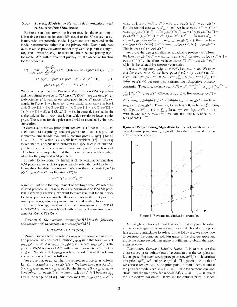
We refer this problem as Revenue Maximization (RM) problemand the optimal revenue for RM as OPT (RM). We use (m, spm[ j])to denote the jth lowest survey price point in the mth model. For ex-ample, in Figure 2, we have six survey participants shown in blackdisk (1, sp1[1] = 1), (1, sp1[2] = 4), (2, sp2[1] = 3), (2, sp2[2] =
7), (3, sp3[1] = 5), and (3, sp3[2] = 8). In general, the smaller theε, the stricter the privacy restriction, which results to lower modelprice. The reason for this price trend will be revealed by the nextsubsection.
Given a set of survey price points (m, spm[1]) for m = 1, 2, ...,M,does there exist a pricing function p(εm) such that 1) is positive,monotone, and subadditive; and 2) ensures p(εm) = spm[1] for allm = 1, 2, ...,M, which is a co-NP hard problem [13]. It is easyto see that this co-NP hard problem is a special case of our RMproblem, i.e., there is only one survey price point for each model.Therefore, it is suspected that there is no polynomial-time algo-rithm for the proposed RM problem.
In order to overcome the hardness of the original optimizationRM problem, we seek to approximately solve the problem by re-laxing the subadditivity constraint. We relax the constraint of p(εm)+p(εm′ ) ≥ p(εm + εm′ ) in Equation (22) to
p(εm)/εm ≥ p(εm′ )/εm′ (23)
which still satisfies the requirement of arbitrage-free. We refer thisrelaxed problem as Relaxed Revenue Maximization (RRM) prob-lem. Generally speaking, we want to make sure that the unit pricefor large purchases is smaller than or equals to the unit price forsmall purchases, which is practical in the real marketplaces.
In the following, we show the maximum revenue for RRM,OPT (RRM), has a lower bound with respect to the maximum rev-enue for RM, OPT (RM).
Theorem 5. The maximum revenue for RM has the followingrelationship with the maximum revenue for RRM
OPT (RRM) ≥ OPT (RM)/2
Proof. Given a feasible solution pRM of the revenue maximiza-tion problem, we construct a solution pRRM such that for all m > 0,pRRM(εm) = εm × min0<x≤mpRM(ε x)/ε x, where pRRM(εm) is theprice in RRM for modelMm with privacy parameter εm. Let 0 <m ≤ m′. We show that pRRM is a feasible solution of the relaxingmaximization problem as follows.
We prove that pRRM satisfies the monotone property as follows.Let x′min = arg min0<x≤m′ pRM(ε x)/ε x. We have two cases for x′min,0 < x′min ≤ m and m < x′min ≤ m′. For the first case 0 < x′min ≤ m, wehave min0<x≤m′ pRM(ε x)/ε x = min0<x≤mpRM(ε x)/ε x because x′minlies in the range of (0,m]. And then we have pRRM(εm′ ) = εm′ ×
min0<x≤m′ pRM(ε x)/ε x ≥ εm × min0<x≤mpRM(ε x)/ε x = pRRM(εm).For the second case m < x′min ≤ m′, we have pRRM(εm) = εm ×
min0<x≤mpRM(ε x)/ε x ≤ εm×pRM(ε x)/ε xx=m = εm×pRM(εm)/εm =
pRM(εm) < pRM(ε x′min ) = ε x′min pRM(ε x′min )/ε x′min . Because x′min ≤
m′ and pRM(ε x′min )/ε x′min = min0<x≤m′ pRM(ε x)/ε x, then we haveε x′min pRM(ε x′min )/ε x′min ≤ εm′ ×min0<x≤m′ pRM(ε x)/ε x = pRRM(εm′ ).That is pRRM(εm) < pRRM(εm′ ).
We prove that pRRM satisfies the subadditive property as follows.We have pRRM(εm)/εm = min0<x≤mpRM(ε x)/ε x ≥ min0<x≤m′ pRM(ε x)/ε x =
pRRM(εm′ )/εm′ . Therefore, we have pRRM(εm)/εm ≥ pRRM(εm′ )/εm′
which is the subadditive property constraint.Let xmin = arg min0<x≤mpRM(ε x)/ε x, i.e., xmin ≤ m. We show
that for every m > 0, we have pRM(εm)/2 ≤ pRRM(εm) as fol-lows. We have pRM(εm) = pRM(ε xmin εm
εxmin ) ≤ pRM(ε xmind εm
εxmin e) ≤d εm
εxmin epRM(ε xmin ) because pRM satisfies the subadditive propertyconstraint. Therefore, we have pRRM(εm) = εm
pRM(εxmin )εxmin ≥ εm
εxmin pRM(εm)
d εmεxmin e
≥
εm
εxmin pRM(εm)εm
εxmin +1 ≥ pRM(εm)/2 because xmin ≤ m. Because pRRM(εm) =
εm × min0<x≤mpRM(εx)
εx ≤ εm × pRM(εx)
εx x=m = pRM(εm), we havepRRM(εm) ≤ pRM(εm). Therefore, for each m > 0, we have
∑K′k=1 ·I(tmk ==
m) · I(pRRM(εm) ≤ vk) ≥∑K′
k=1 ·I(tmk == m) · I(pRM(εm) ≤ vk).With pRM(εm)/2 ≤ pRRM(εm), we conclude that OPT (RM)/2 ≤OPT (RRM).
Dynamic Programming Algorithm. In this part, we show an effi-cient dynamic programming algorithm to solve the relaxed revenuemaximization problem.
1
4
3
7
5
8
5
10
1 2 30
price
ǫ
Figure 2: Revenue maximization example.
At first glance, for each model, it seems that all possible valuesin the price range can be an optimal price, which makes the prob-lem arguably intractable to solve. In the following, we show howto construct the complete solution space in the discrete space andprove the complete solution space is sufficient to obtain the maxi-mum revenue.
Constructing Complete Solution Space. It is easy to see thatthose survey price points should be contained in the complete so-lution space. For each survey price point (m, spm[ j]), it determinesunit price spm[ j]/εm and price spm[ j]. The general idea is that ifwe choose (m, spm[ j]) as the price point in model Mm, it affectsthe price for modelsMk, k = 1, ...,m − 1 due to the monotone con-straint and the unit price for models Mk, k = m + 1, ...,M due tothe subadditive constraint. If we set the optimal price in model
12
Mm as spm[ j], the unit price of the following models after modelMm cannot be larger than spm[ j]/εm. Therefore, for each surveyprice point (m, spm[ j]), we draw one line l(m,spm[ j]) through sur-vey price point (m, spm[ j]) and the original point. For each modelMm, we draw one vertical line lMm . By intersecting line l(m,spm[ j])
and lMm , we obtain M − m new price points (lMk , l(m,spm[ j])) fork = m + 1, ...,M. We note that we do not need to generate theprice points for k = 1, ...,m−1 because the unit price of modelMm
can only constrain the unite price of model Mk, k = m + 1, ...,M.Furthermore, for each model, its price is also determined by thesurvey price of its right neighbors. Therefore, we need to add thesurvey price points of model Mm to models Mk, k = 1, ...,m − 1.The detailed algorithm for constructing the complete solution spaceis shown in Algorithm 6. In Lines 11-15, we use f (m, pm[ j]) to dis-tinguish the survey price points from the other points in the com-plete solution space. For ease of presentation in the following, wename the price point in the complete solution space from Line 1as SV (survey) point, the price point from Line 8 as SC (subad-ditivity constraint) point, and the price point from Line 10 asMC(monotonicity constraint) point.
Algorithm 6: Constructing complete solution space for the re-laxed revenue maximization problem.
input : Model with noise parameter εm and the jth lowestsurvey price point for model with noise parameter εm,denoted as (m, spm[ j]).
output: Complete solution space.1 add all the survey price points (m, spm[ j]) to the complete
solution space;2 for each survey price point (m, spm[ j]) do3 draw a line l(m,spm[ j]) through this point and the original
point;
4 for each model with noise parameter εm do5 draw a vertical line lMm ;
6 for each line lMm do7 for each line l(m,spm[ j]) do8 add point (lMk , l(m,spm[ j])) by intersecting line lMm and
line l(m,spm[ j]) to the complete solution space fork = m + 1, ...,M;
9 for each survey price point (m, spm[ j]) do10 add price point (k, spm[ j]) to the complete solution space
for k = 1, ...,m − 1;
11 for each price point (m, pm[ j]) in the complete solution spacedo
12 if (m, pm[ j]) is a survey price point then13 f (m, pm[ j]) = 1;
14 else15 f (m, pm[ j]) = 0;
Example 1. We show an running example of Algorithm 6. InFigure 2, we assume ε1 = 1, ε2 = 2, and ε3 = 3. We add thesurvey price points (1, sp1[1] = 1), (1, sp1[2] = 4), (2, sp2[1] = 3),(2, sp2[2] = 7), (3, sp3[1] = 5), and (3, sp3[2] = 8) to the completesolution space in Line 1. In Line 2, for the survey price point (1, 1),we draw a line l(1,1) through this point and the original point inLine 3. In Line 4, for model M1 with noise parameter ε1 = 1,we draw a vertical line lM1 . In Lines 6-8, for l1,1 and lM2 , we addintersection (lM2 , l1,sp1[1]) = (2, 2) to the complete solution space.In total, we have six such new price points shown in box. In Line 9,
for survey price point (3, sp3[1]) = (3, 5), we add price points (2, 5)and (1, 5) to the complete solution space in Line 10. Similarly, wealso have six such new price points shown in circle. Therefore, forthe complete solution space, we have six price points for modelsM1 andM3. We have five price points for modelM2 because theintersection point of lM2 , l1,sp1[2] = (2, 8) is same to theMC point(k, sp3[2]) = (2, 8) for k = 2. In Lines 12-15, we have f (2, 3) = 1and f (2, 5) = 0.
Theorem 6. The complete solution space constructed by Algo-rithm 6 is sufficient for finding the optimal solution of the relaxedrevenue maximization problem.
Proof. As we discussed in constructing complete solution space,for each survey price point (m, spm[ j]), it can affect the model rev-enue of modelMm, the unit price for modelsMk, k = m + 1, ...,Mand the price for models Mk, k = 1, ...,m − 1. We prove that theSC andMC points are non-recursive, i.e., we do not need to gen-erate new price points in the complete solution space based on thegenerated SC andMC points.
Given a survey price point (m, spm[ j]) in model Mm, it deter-mines aSC point in modelMm′ , where m′ > m, i.e., (m′, spm[ j]/εm×
εm′ ). We do not need to generateSC points based on (m′, spm[ j]/εm×
εm′ ) because it has the same SC points for models Mk, k = m′ +
1, ...,M with (m, spm[ j]). We may use (m′, spm[ j]/εm × εm′ ) to gen-erate a MC point (k, spm[ j]/εm × εm′ ). If k > m, the new point(k, spm[ j]/εm × εm′ ) is not necessary because spm[ j]/εm × εm′/εk >spm[ j]/εm which violates the subadditive constraint. If k < m,the new point (k, spm[ j]/εm × εm′ ) is also not necessary becausespm[ j]/εm× εm′ > spm[ j] which violates the subadditive constraint.
Given a survey price point (m, spm[ j]) in model Mm, it deter-mines aMC point in modelMm′ , where m′ < m, i.e., (m′, spm[ j]).We do not need to generate MC points based on (m′, spm[ j]) be-cause those MC points are already determined by (m, spm[ j]). Itis also not necessary to generate SC points based on (m′, spm[ j])because if (m′, spm[ j]) and (m, spm[ j]) are chosen as the optimalprices, all the optimal prices for modelsMk, k = m′, ...m, ...,M aredetermined, i.e., p(εm′ ) = ... = p(εm) = ...p(εM).
A recursive solution. We define the revenue of an optimal solu-tion recursively in terms of the optimal solutions to subproblems.We pick as our subproblems the problems of determining the max-imum revenue OPT (m, j), where OPT (m, j) denotes the maximumrevenue for considering the first m models and taking the jth low-est price point in the complete solution space of model Mm. Forthe full problem, the maximum revenue would be maxOPT (M, j)for all the price points (M, pM[ j]) in the complete solution spacein modelMM . For the price points in the complete solution spaceof modelM1, we can directly compute OPT (1, j) for all the pricepoints because there is no initial constraint. For the price points inthe complete solution space of other models, we need to considerboth the monotone constraint and the subadditive constraint. Wehave a recursive equation as follows.
OPT (m, j) = maxOPT (m − 1, j′) + MR(m, j) (24)
where pm−1[ j′] ≤ pm[ j]&&pm−1[ j′]/εm−1 ≥ pm[ j]/εm and MR(m, j)denotes the revenue from model Mm if we price model Mm forpm[ j].
Computing the maximum revenue. Now, we could easily write arecursive algorithm in Algorithm 7 based on recurrence (24), where|pm| is the number of the price points in modelMm.
Theorem 7. Algorithm 7 can be finished in O(N2 M2) time.
13
Algorithm 7: Dynamic programming algorithm for finding anoptimal solution of the relaxed revenue maximization problem.
input : Model with noise parameter εm and its correspondingprice points in the complete solution space.
output: OPT (RRM).1 for each modelMm do2 sort the price points in the complete solution space in
decreasing order;3 use (m, pm[ j]) to denote the jth lowest price point;4 MR(m, |pm|) = pm[|pm|] f (m, pm[|pm|]);5 for j = |pm| − 1 to 1 do6 MR(m, j) = pm[ j]
∑|pm |k= j f (m, pm[k]);
7 for j = 1 to |p1| do8 OPT (1, j) = MR(1, p1[ j]);
9 for each modelMm,m = 2, ...,M do10 for each price point (m, pm[ j]) do11 OPT (m, j) = maxOPT (m − 1, j′) + MR(m, j), where
pm−1[ j′] ≤ pm[ j]&&pm−1[ j′]/εm−1 ≥ pm[ j]/εm;12 p(L.OPT (m, j)) = pm−1[ j′] that satisfies OPT (m, j) in
Line 11;
13 OPT (RRM) = maxOPT (M, j), where j = 1 to |pm|.
Proof. For the O(N) survey price points, we general O(NM)price points in the complete solution space. For each price pointin the complete solution space, we need O(NM) time to updateOPT (m, j). Therefore, Algorithm 7 requires O(N2 M2) time.
Example 2. In model M1 of Figure 2, we have OPT (1, j) forj = 1, 2, ..., 6 shown in Table 2. For computing OPT (2, 2), there isonly one price point (1, 3) satisfying both the monotone constraintand the subadditive constraint within model M1. Therefore, wehave OPT (2, 2) = OPT (1, 2) + MR(2, 2) = 3 + 6 = 9. Similarly, wecan fill the entire table shown in Table 2.
Constructing an optimal solution. Although Algorithm 7 deter-mines the maximum revenue of RRM, it does not directly showthe optimal price for each model p(εm). However, for each pricepoint (m, pm[ j]) in the complete solution space, we record the pricepoint p(L.OPT (m, j)) in modelMm−1 which has the maximum rev-enue in those price points that satisfy both the monotone constraintand the subadditive constraint with (m, pm[ j]) in Line 12 of Algo-rithm 7. Therefore, we can recursively backtrack the optimal pricepoint in model Mm−1 from the optimal price point in model Mm.We need O(nM) time to find the maximum value in OPT (M, j) andO(M) time to backtrack. Therefore, we can construct an optimalsolution in O(NM) time. We note that such a solution may be oneof several solutions that can achieve the optimal value.
We show an running example in Table 2. We first obtain OPT (3, 3)which has the maximum value among OPT (3, j) for j = 1, 2, ..., 6.Therefore, we set p(ε3) = 5. We backtrack to OPT (2, 2) in modelM2 and set p(ε2) = 3. And then we backtrack to OPT (1, 2) inmodel M1 and set p(ε1) = 3. Finally, an optimal pricing settingis 〈p(ε1), p(ε2), p(ε3)〉 = 〈3, 3, 5〉. We note that in our running ex-ample, the pricing setting 〈4, 5, 5〉 also has the maximum revenue19.
Assumption 4. The broker is honest but curious.
Remark 3. In practice, the broker may be semi-honest or evenmalicious. For these cases, we can take advantage of the local
Table 2: Example for constructing an optimal solution.
Model# of points
1 2 3 4 5 6
M1 2 3 4 0 0 0M2 6 9 9 11 4 NullM3 15 18 19 19 11 4
differential privacy [15] in which the data owners and the modelbuyers can add DP noise by themselves before sending their datato the broker. Also, encryption-based techniques can be furtherincorporated into the market design.
5.4 Complete Differentially Private Data Mar-ketplace Dynamics
We summarize the differentially private data marketplace withmodel-based pricing dynamics from the broker’s perspective, whichis an end-to-end data marketplace with practical considerations andconsists of computationally efficient component algorithms. Thedetailed algorithm is shown in Algorithm 8, which integrates allthe proposed algorithms in the previous sections. We assume thatthe broker can set appropriate parameters M, εm, andMBm basedon her market experiences, which is reasonable. For example, Mi-crosoft can easily determine the different features assigned to Win-dows 10 Home version and Windows 10 Pro version. Finally, al-though instantiated with the DP market, we stress that Algorithm 8can be applied to the general setting by switching the DP parameterto the risk factor.
Algorithm 8: The complete broker functioning in DP-DealerPipeline.
1 collect data and usage restriction among n data owners: collectdataset D = zi along with DP restriction parameters εi andextra compensation function eci for i = 1, 2, ..., n;
2 decide a set of M models to train with model privacy parameterεm and manufacturing budgetMBm for m = 1, 2, ...,M;
3 %% Model training and releasing;4 for m=1 to M do5 data valuation: call Algorithm 1 to compute approximate
Shapley value SVmi for i = 1, 2, ..., n;
6 base compensation: compute bcmi =
SVmi∑n
i=1 SVmiMB
m;
7 data selection: call Algorithm 3, 4, or 5 to select trainingsubset Sm with manufacturing budgetMBm to maximizeSV(Sm);
8 model training: train the model with subset Sm byAlgorithm 2;
9 model releasing: release modelMm, its pricing p(εm) andestimated excess population loss ∆L(Am
Algorithm2; εm,Sm);
10 perform market survey among K′ sampling model buyers(survey participants): collect market survey results of modeldemand tmk and valuation vk for k = 1, 2, ...,K′;
11 %% Model pricing;12 model pricing: call Algorithms 6 and 7 to compute the optimal
price p(εm) of modelMm for m = 1, 2, ...,M;13 %% Compensation allocation;14 for m=1 to M do15 compute bci and eci of data owner Oi for i ∈ Sm by
proportionally dividing p(εm)∑Mm=1 p(εm)
OPT (RRM) and allocate
the corresponding compensation to Oi;
14
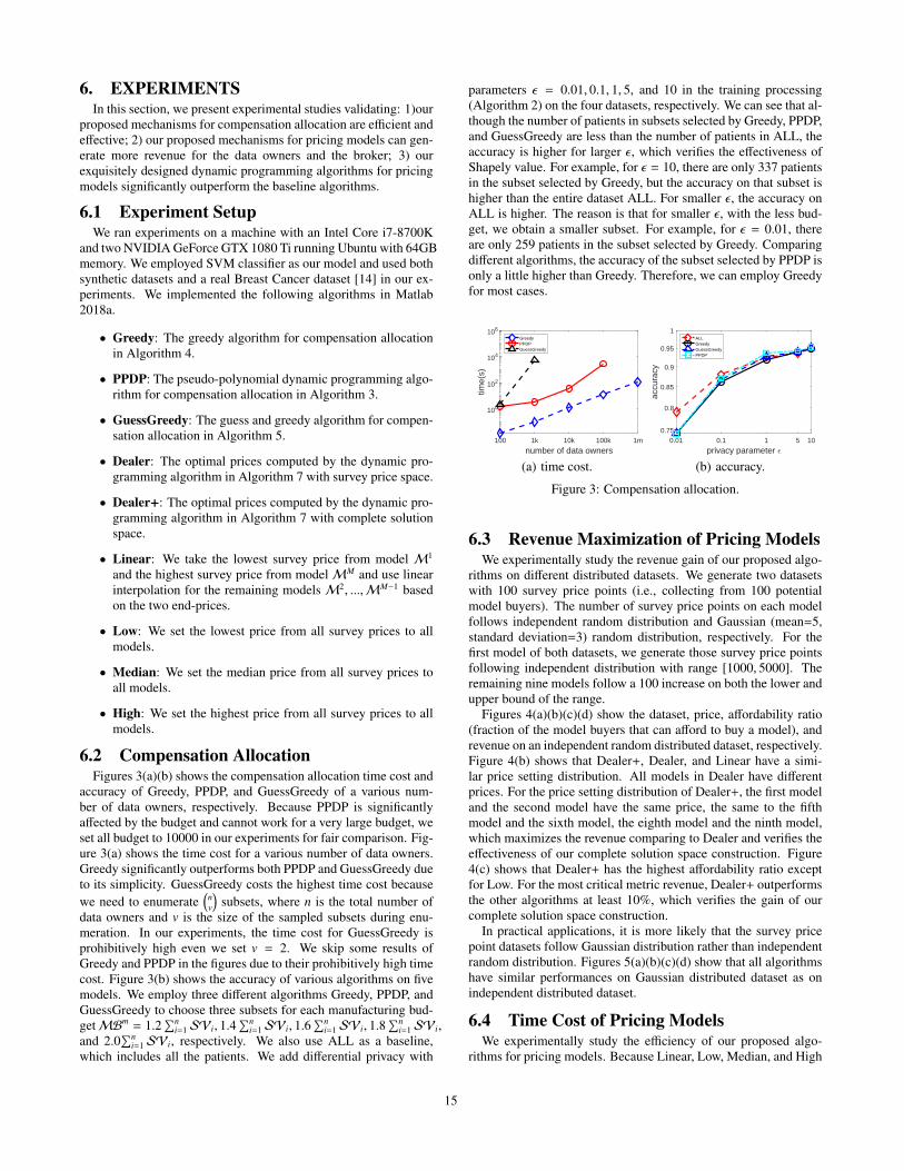
6. EXPERIMENTSIn this section, we present experimental studies validating: 1)our
proposed mechanisms for compensation allocation are efficient andeffective; 2) our proposed mechanisms for pricing models can gen-erate more revenue for the data owners and the broker; 3) ourexquisitely designed dynamic programming algorithms for pricingmodels significantly outperform the baseline algorithms.
6.1 Experiment SetupWe ran experiments on a machine with an Intel Core i7-8700K
and two NVIDIA GeForce GTX 1080 Ti running Ubuntu with 64GBmemory. We employed SVM classifier as our model and used bothsynthetic datasets and a real Breast Cancer dataset [14] in our ex-periments. We implemented the following algorithms in Matlab2018a.
• Greedy: The greedy algorithm for compensation allocationin Algorithm 4.
• PPDP: The pseudo-polynomial dynamic programming algo-rithm for compensation allocation in Algorithm 3.
• GuessGreedy: The guess and greedy algorithm for compen-sation allocation in Algorithm 5.
• Dealer: The optimal prices computed by the dynamic pro-gramming algorithm in Algorithm 7 with survey price space.
• Dealer+: The optimal prices computed by the dynamic pro-gramming algorithm in Algorithm 7 with complete solutionspace.
• Linear: We take the lowest survey price from model M1
and the highest survey price from modelMM and use linearinterpolation for the remaining models M2, ...,MM−1 basedon the two end-prices.
• Low: We set the lowest price from all survey prices to allmodels.
• Median: We set the median price from all survey prices toall models.
• High: We set the highest price from all survey prices to allmodels.
6.2 Compensation AllocationFigures 3(a)(b) shows the compensation allocation time cost and
accuracy of Greedy, PPDP, and GuessGreedy of a various num-ber of data owners, respectively. Because PPDP is significantlyaffected by the budget and cannot work for a very large budget, weset all budget to 10000 in our experiments for fair comparison. Fig-ure 3(a) shows the time cost for a various number of data owners.Greedy significantly outperforms both PPDP and GuessGreedy dueto its simplicity. GuessGreedy costs the highest time cost becausewe need to enumerate
(nv
)subsets, where n is the total number of
data owners and v is the size of the sampled subsets during enu-meration. In our experiments, the time cost for GuessGreedy isprohibitively high even we set v = 2. We skip some results ofGreedy and PPDP in the figures due to their prohibitively high timecost. Figure 3(b) shows the accuracy of various algorithms on fivemodels. We employ three different algorithms Greedy, PPDP, andGuessGreedy to choose three subsets for each manufacturing bud-getMBm = 1.2
∑ni=1 SVi, 1.4
∑ni=1 SVi, 1.6
∑ni=1 SVi, 1.8
∑ni=1 SVi,
and 2.0∑n
i=1 SVi, respectively. We also use ALL as a baseline,which includes all the patients. We add differential privacy with
parameters ε = 0.01, 0.1, 1, 5, and 10 in the training processing(Algorithm 2) on the four datasets, respectively. We can see that al-though the number of patients in subsets selected by Greedy, PPDP,and GuessGreedy are less than the number of patients in ALL, theaccuracy is higher for larger ε, which verifies the effectiveness ofShapely value. For example, for ε = 10, there are only 337 patientsin the subset selected by Greedy, but the accuracy on that subset ishigher than the entire dataset ALL. For smaller ε, the accuracy onALL is higher. The reason is that for smaller ε, with the less bud-get, we obtain a smaller subset. For example, for ε = 0.01, thereare only 259 patients in the subset selected by Greedy. Comparingdifferent algorithms, the accuracy of the subset selected by PPDP isonly a little higher than Greedy. Therefore, we can employ Greedyfor most cases.
100 1k 10k 100k 1m
number of data owners
100
102
104
106
time(
s)
GreedyPPDPGuessGreedy
(a) time cost.
0.01 0.1 1 5 10
privacy parameter
0.75
0.8
0.85
0.9
0.95
1
accu
racy
ALLGreedyGuessGreedyPPDP
(b) accuracy.
Figure 3: Compensation allocation.
6.3 Revenue Maximization of Pricing ModelsWe experimentally study the revenue gain of our proposed algo-
rithms on different distributed datasets. We generate two datasetswith 100 survey price points (i.e., collecting from 100 potentialmodel buyers). The number of survey price points on each modelfollows independent random distribution and Gaussian (mean=5,standard deviation=3) random distribution, respectively. For thefirst model of both datasets, we generate those survey price pointsfollowing independent distribution with range [1000, 5000]. Theremaining nine models follow a 100 increase on both the lower andupper bound of the range.
Figures 4(a)(b)(c)(d) show the dataset, price, affordability ratio(fraction of the model buyers that can afford to buy a model), andrevenue on an independent random distributed dataset, respectively.Figure 4(b) shows that Dealer+, Dealer, and Linear have a simi-lar price setting distribution. All models in Dealer have differentprices. For the price setting distribution of Dealer+, the first modeland the second model have the same price, the same to the fifthmodel and the sixth model, the eighth model and the ninth model,which maximizes the revenue comparing to Dealer and verifies theeffectiveness of our complete solution space construction. Figure4(c) shows that Dealer+ has the highest affordability ratio exceptfor Low. For the most critical metric revenue, Dealer+ outperformsthe other algorithms at least 10%, which verifies the gain of ourcomplete solution space construction.
In practical applications, it is more likely that the survey pricepoint datasets follow Gaussian distribution rather than independentrandom distribution. Figures 5(a)(b)(c)(d) show that all algorithmshave similar performances on Gaussian distributed dataset as onindependent distributed dataset.
6.4 Time Cost of Pricing ModelsWe experimentally study the efficiency of our proposed algo-
rithms for pricing models. Because Linear, Low, Median, and High
15
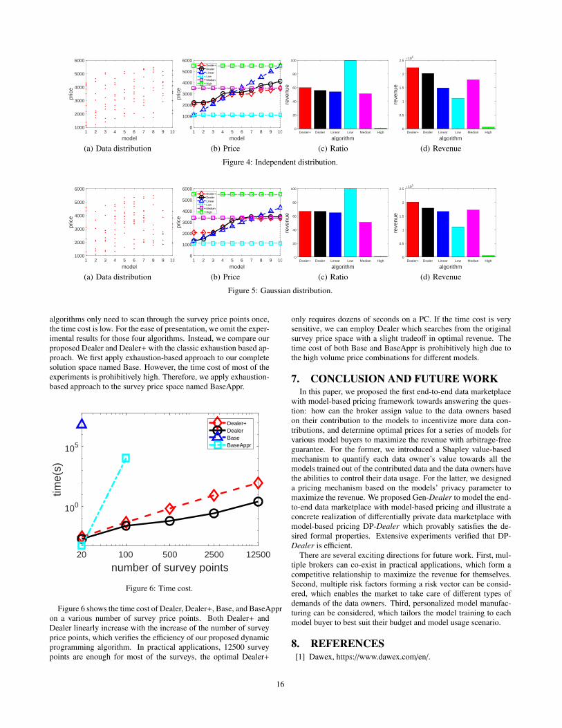
1 2 3 4 5 6 7 8 9 10
model
1000
2000
3000
4000
5000
6000
pric
e
(a) Data distribution
1 2 3 4 5 6 7 8 9 10
model
0
1000
2000
3000
4000
5000
6000
pric
e
Dealer+DealerLinearLowMedianHigh
(b) Price
Dealer+ Dealer Linear Low Median High
algorithm
0
20
40
60
80
100
reve
nue
(c) Ratio
Dealer+ Dealer Linear Low Median High
algorithm
0
0.5
1
1.5
2
2.5
reve
nue
105
(d) Revenue
Figure 4: Independent distribution.
1 2 3 4 5 6 7 8 9 10
model
1000
2000
3000
4000
5000
6000
pric
e
(a) Data distribution
1 2 3 4 5 6 7 8 9 10
model
0
1000
2000
3000
4000
5000
6000
pric
e
Dealer+DealerLinearLowMedianHigh
(b) Price
Dealer+ Dealer Linear Low Median High
algorithm
0
20
40
60
80
100
reve
nue
(c) Ratio
Dealer+ Dealer Linear Low Median High
algorithm
0
0.5
1
1.5
2
2.5
reve
nue
105
(d) Revenue
Figure 5: Gaussian distribution.
algorithms only need to scan through the survey price points once,the time cost is low. For the ease of presentation, we omit the exper-imental results for those four algorithms. Instead, we compare ourproposed Dealer and Dealer+ with the classic exhaustion based ap-proach. We first apply exhaustion-based approach to our completesolution space named Base. However, the time cost of most of theexperiments is prohibitively high. Therefore, we apply exhaustion-based approach to the survey price space named BaseAppr.
20 100 500 2500 12500
number of survey points
100
105
time(
s)
Dealer+DealerBaseBaseAppr
Figure 6: Time cost.
Figure 6 shows the time cost of Dealer, Dealer+, Base, and BaseAppron a various number of survey price points. Both Dealer+ andDealer linearly increase with the increase of the number of surveyprice points, which verifies the efficiency of our proposed dynamicprogramming algorithm. In practical applications, 12500 surveypoints are enough for most of the surveys, the optimal Dealer+
only requires dozens of seconds on a PC. If the time cost is verysensitive, we can employ Dealer which searches from the originalsurvey price space with a slight tradeoff in optimal revenue. Thetime cost of both Base and BaseAppr is prohibitively high due tothe high volume price combinations for different models.
7. CONCLUSION AND FUTURE WORKIn this paper, we proposed the first end-to-end data marketplace
with model-based pricing framework towards answering the ques-tion: how can the broker assign value to the data owners basedon their contribution to the models to incentivize more data con-tributions, and determine optimal prices for a series of models forvarious model buyers to maximize the revenue with arbitrage-freeguarantee. For the former, we introduced a Shapley value-basedmechanism to quantify each data owner’s value towards all themodels trained out of the contributed data and the data owners havethe abilities to control their data usage. For the latter, we designeda pricing mechanism based on the models’ privacy parameter tomaximize the revenue. We proposed Gen-Dealer to model the end-to-end data marketplace with model-based pricing and illustrate aconcrete realization of differentially private data marketplace withmodel-based pricing DP-Dealer which provably satisfies the de-sired formal properties. Extensive experiments verified that DP-Dealer is efficient.
There are several exciting directions for future work. First, mul-tiple brokers can co-exist in practical applications, which form acompetitive relationship to maximize the revenue for themselves.Second, multiple risk factors forming a risk vector can be consid-ered, which enables the market to take care of different types ofdemands of the data owners. Third, personalized model manufac-turing can be considered, which tailors the model training to eachmodel buyer to best suit their budget and model usage scenario.
8. REFERENCES[1] Dawex, https://www.dawex.com/en/.
16
[2] Google bigquery, https://cloud.google.com/bigquery/.[3] https://support.gnip.com/apis/.[4] https://www.bloomberg.com/professional/product/market-
data/.[5] Iota, https://data.iota.org/.[6] A. Agarwal, M. Dahleh, and T. Sarkar. A marketplace for
data: An algorithmic solution. In Proceedings of the 2019ACM Conference on Economics and Computation, pages701–726. ACM, 2019.
[7] S. Alaei, A. Malekian, and A. Srinivasan. On randomsampling auctions for digital goods. ACM Trans. Economicsand Comput., 2(3):11:1–11:19, 2014.
[8] M. Ancona, C. Oztireli, and M. H. Gross. Explaining deepneural networks with a polynomial time algorithm forshapley value approximation. In Proceedings of the 36thInternational Conference on Machine Learning, ICML 2019,9-15 June 2019, Long Beach, California, USA, pages272–281, 2019.
[9] R. Bassily, V. Feldman, K. Talwar, and A. G. Thakurta.Private stochastic convex optimization with optimal rates. InAdvances in Neural Information Processing Systems, pages11279–11288, 2019.
[10] J. Castro, D. Gomez, and J. Tejada. Polynomial calculationof the shapley value based on sampling. Computers & OR,36(5):1726–1730, 2009.
[11] G. C. Cawley and N. L. C. Talbot. Efficient leave-one-outcross-validation of kernel fisher discriminant classifiers.Pattern Recognition, 36(11):2585–2592, 2003.
[12] S. Chawla, S. Deep, P. Koutris, and Y. Teng. Revenuemaximization for query pricing. PVLDB, 13(1):1–14, 2019.
[13] L. Chen, P. Koutris, and A. Kumar. Towards model-basedpricing for machine learning in a data marketplace. InProceedings of the 2019 International Conference onManagement of Data, SIGMOD Conference 2019,Amsterdam, The Netherlands, June 30 - July 5, 2019., pages1535–1552, 2019.
[14] D. Dua and C. Graff. UCI machine learning repository, 2017.[15] J. C. Duchi, M. I. Jordan, and M. J. Wainwright. Local
privacy and statistical minimax rates. In 54th Annual IEEESymposium on Foundations of Computer Science, FOCS2013, 26-29 October, 2013, Berkeley, CA, USA, pages429–438, 2013.
[16] C. Dwork, F. McSherry, K. Nissim, and A. Smith.Calibrating noise to sensitivity in private data analysis. InTheory of cryptography conference, pages 265–284.Springer, 2006.
[17] C. Dwork, A. Roth, et al. The algorithmic foundations ofdifferential privacy. Foundations and Trends R© in TheoreticalComputer Science, 9(3–4):211–407, 2014.
[18] S. S. Fatima, M. J. Wooldridge, and N. R. Jennings. A linearapproximation method for the shapley value. Artif. Intell.,172(14):1673–1699, 2008.
[19] A. Ghorbani and J. Y. Zou. Data shapley: Equitable valuationof data for machine learning. In Proceedings of the 36th
International Conference on Machine Learning, ICML 2019,9-15 June 2019, Long Beach, California, USA, pages2242–2251, 2019.
[20] A. Ghosh and A. Roth. Selling privacy at auction. InProceedings 12th ACM Conference on Electronic Commerce(EC-2011), San Jose, CA, USA, June 5-9, 2011, pages199–208, 2011.
[21] V. Guruswami, J. D. Hartline, A. R. Karlin, D. Kempe,C. Kenyon, and F. McSherry. On profit-maximizingenvy-free pricing. In Proceedings of the Sixteenth AnnualACM-SIAM Symposium on Discrete Algorithms, SODA2005, Vancouver, British Columbia, Canada, January 23-25,2005, pages 1164–1173, 2005.
[22] R. Iyengar, J. P. Near, D. Song, O. Thakkar, A. Thakurta, andL. Wang. Towards practical differentially private convexoptimization. In IEEE S and P.
[23] B. Jayaraman and D. Evans. Evaluating differentially privatemachine learning in practice. In 28th USENIX SecuritySymposium, USENIX Security 2019, Santa Clara, CA, USA,August 14-16, 2019, pages 1895–1912, 2019.
[24] R. Jia, D. Dao, B. Wang, F. A. Hubis, N. M. Gurel, B. Li,C. Zhang, C. Spanos, and D. Song. Efficient task-specificdata valuation for nearest neighbor algorithms. Proceedingsof the VLDB Endowment, 12(11):1610–1623, 2019.
[25] P. Koutris, P. Upadhyaya, M. Balazinska, B. Howe, andD. Suciu. Query-based data pricing. In Proceedings of the31st ACM SIGMOD-SIGACT-SIGAI symposium onPrinciples of Database Systems, pages 167–178. ACM,2012.
[26] P. Koutris, P. Upadhyaya, M. Balazinska, B. Howe, andD. Suciu. Toward practical query pricing with querymarket.In proceedings of the 2013 ACM SIGMOD internationalconference on management of data, pages 613–624. ACM,2013.
[27] P. Koutris, P. Upadhyaya, M. Balazinska, B. Howe, andD. Suciu. Query-based data pricing. J. ACM,62(5):43:1–43:44, 2015.
[28] C. Li, D. Y. Li, G. Miklau, and D. Suciu. A theory of pricingprivate data. In Joint 2013 EDBT/ICDT Conferences, ICDT’13 Proceedings, Genoa, Italy, March 18-22, 2013, pages33–44, 2013.
[29] C. Li, D. Y. Li, G. Miklau, and D. Suciu. A theory of pricingprivate data. ACM Trans. Database Syst., 39(4):34:1–34:28,2014.
[30] C. Li, D. Y. Li, G. Miklau, and D. Suciu. A theory of pricingprivate data. Commun. ACM, 60(12):79–86, 2017.
[31] B. Lin and D. Kifer. On arbitrage-free pricing for generaldata queries. PVLDB, 7(9):757–768, 2014.
[32] C. Shapiro and H. Varian. Versioning: The smart way to sellinformation. Harvard Business Review, 76(6):107–115,1998.
[33] L. S. Shapley. A value for n-person games. Contributions tothe Theory of Games, 2(28):307–317, 1953.
17