dealing with and understanding endogeneity · dealing with and understanding endogeneity enrique...
TRANSCRIPT

Dealing With and Understanding Endogeneity
Enrique Pinzón
StataCorp LP
October 20, 2016Barcelona
(StataCorp LP) October 20, 2016 Barcelona 1 / 59

Importance of Endogeneity
Endogeneity occurs when a variable, observed or unobserved,that is not included in our models, is related to a variable weincorporated in our model.
Model buildingEndogeneity contradicts:
I Unobservables have no effect or explanatory powerI The covariates cause the outcome of interest
Endogeneity prevents us from making causal claimsEndogeneity is a fundamental concern of social scientists (first tothe party)
(StataCorp LP) October 20, 2016 Barcelona 2 / 59

Outline
1 Defining concepts and building our intuition2 Stata built in tools to solve endogeneity problems3 Stata commands to address endogeneity in non-built-in situations
(StataCorp LP) October 20, 2016 Barcelona 3 / 59

Defining concepts and building our intuition
(StataCorp LP) October 20, 2016 Barcelona 4 / 59
Building our Intuition: A Regression Model
The regression model is given by:
yi = β0 + β1x1i + . . .+ βkxki + εi
E (εi |x1i , . . . , xki) = 0
Once we have the information of our regressors, on average whatwe did not include in our model has no importance.
E (yi |x1i , . . . , xki) = β0 + β1x1i + . . .+ βkxki
(StataCorp LP) October 20, 2016 Barcelona 5 / 59

Graphically
(StataCorp LP) October 20, 2016 Barcelona 6 / 59

Examples of Endogeneity
We want to explain wages and we use years of schooling as acovariate. Years of schooling is correlated with unobserved ability,and work ethic.We want to explain to probability of divorce and use employmentstatus as a covariate. Employment status might be correlated tounobserved economic shocks.We want to explain graduation rates for different school districtsand use the fraction of the budget used in education as acovariate. Budget decisions are correlated to unobservablepolitical factors.Estimating demand for a good using prices. Demand and pricesare determined simultaneously.
(StataCorp LP) October 20, 2016 Barcelona 7 / 59

A General Framework
If the unobservables, what we did not include in our model iscorrelated to our covariates then:
E (ε|X ) 6= 0
Omitted variable “bias”SimultaneityFunctional form misspecificationSelection “bias”
A useful implication of the above condition
E(X ′ε)6= 0
(StataCorp LP) October 20, 2016 Barcelona 8 / 59

Example 1: Omitted Variable “Bias”
The true model is given by
y = β0 + β1x1 + β2x2 + ε
E (ε|x1, x2) = 0
the researcher does not incorporate x2, i.e. they think
y = β0 + β1x1 + ν
The objective is to estimate β1. In our framework we get a consistentestimate if
E (ν|x1) = 0
(StataCorp LP) October 20, 2016 Barcelona 9 / 59
Example 1: Endogeneity
Using the definition of the true model
y = β0 + β1x1 + β2x2 + ε
E (ε|x1, x2) = 0
We know thatν = β2x2 + ε
andE (ν|x1) = β2E (x2|x1)
E (ν|x1) = 0 only if β2 = 0 or x2 and x1 are uncorrelated
(StataCorp LP) October 20, 2016 Barcelona 10 / 59

Example 1: Endogeneity
Using the definition of the true model
y = β0 + β1x1 + β2x2 + ε
E (ε|x1, x2) = 0
We know thatν = β2x2 + ε
andE (ν|x1) = β2E (x2|x1)
E (ν|x1) = 0 only if β2 = 0 or x2 and x1 are uncorrelated
(StataCorp LP) October 20, 2016 Barcelona 10 / 59

Example 1 Simulating Data
. clear. set obs 10000number of observations (_N) was 0, now 10,000. set seed 111. // Generating a common component for x1 and x2. generate a = rchi2(1). // Generating x1 and x2. generate x1 = rnormal() + a. generate x2 = rchi2(2)-3 + a. generate e = rchi2(1) - 1. // Generating the outcome. generate y = 1 - x1 + x2 + e
(StataCorp LP) October 20, 2016 Barcelona 11 / 59
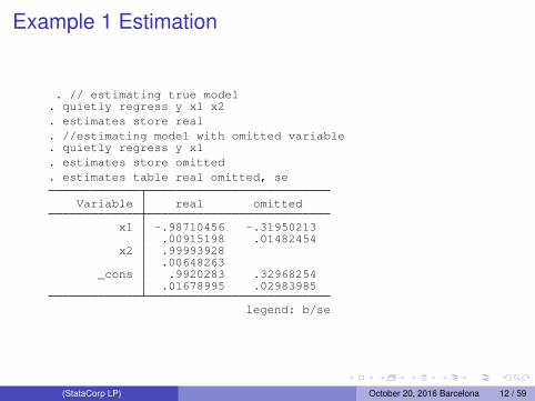
Example 1 Estimation
. // estimating true model. quietly regress y x1 x2. estimates store real. //estimating model with omitted variable. quietly regress y x1. estimates store omitted. estimates table real omitted, se
Variable real omitted
x1 -.98710456 -.31950213.00915198 .01482454
x2 .99993928.00648263
_cons .9920283 .32968254.01678995 .02983985
legend: b/se
(StataCorp LP) October 20, 2016 Barcelona 12 / 59
Example 2: Simultaneity in a market equilibrium
The demand and supply equations for the market are given by
Qd = βPd + εd
Qs = θPs + εs
If a researcher wants to estimate Qd and ignores that Pd issimultaneously determined, we have an endogeneity problem that fitsin our framework.
(StataCorp LP) October 20, 2016 Barcelona 13 / 59

Example 2: Assumptions and Equilibrium
We assume:All quantities are scalarsβ < 0 and θ > 0E (εd ) = E (εs) = E (εdεs) = 0E(ε2
d)≡ σ2
d
The equilibrium prices and quantities are given by:
P =εs − εd
β − θ
Q =βεs − θεd
β − θ
(StataCorp LP) October 20, 2016 Barcelona 14 / 59

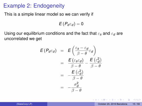
Example 2: EndogeneityThis is a simple linear model so we can verify if
E (Pdεd ) = 0
Using our equilibrium conditions and the fact that εs and εd areuncorrelated we get
E (Pdεd ) = E(εs − εd
β − θεd
)=
E (εsεd )
β − θ−
E(ε2
d)
β − θ
= −E(ε2
d)
β − θ
= −σ2
dβ − θ
(StataCorp LP) October 20, 2016 Barcelona 15 / 59
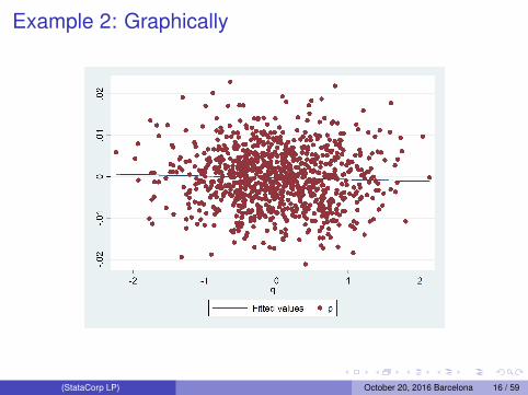
Example 2: Graphically
(StataCorp LP) October 20, 2016 Barcelona 16 / 59
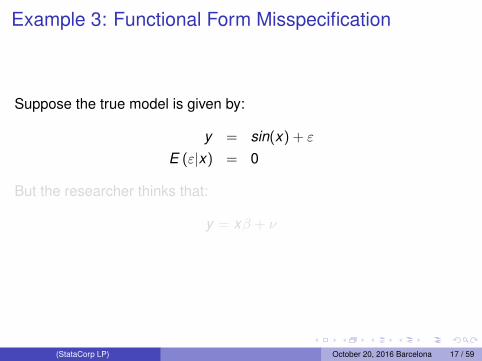
Example 3: Functional Form Misspecification
Suppose the true model is given by:
y = sin(x) + ε
E (ε|x) = 0
But the researcher thinks that:
y = xβ + ν
(StataCorp LP) October 20, 2016 Barcelona 17 / 59

Example 3: Functional Form Misspecification
Suppose the true model is given by:
y = sin(x) + ε
E (ε|x) = 0
But the researcher thinks that:
y = xβ + ν
(StataCorp LP) October 20, 2016 Barcelona 17 / 59

Example 3: Real vs. Estimated Predicted values
(StataCorp LP) October 20, 2016 Barcelona 18 / 59

Example 3: Endogeneity
Adding zero we have
y = xβ − xβ + sin(x) + ε
y = xβ + ν
ν ≡ sin(x)− xβ + ε
For our estimates to be consistent we need to have E (ν|X ) = 0 but
E (ν|x) = sin(x)− xβ + E (ε|x)
= sin(x)− xβ6= 0
(StataCorp LP) October 20, 2016 Barcelona 19 / 59

Example 3: Endogeneity
Adding zero we have
y = xβ − xβ + sin(x) + ε
y = xβ + ν
ν ≡ sin(x)− xβ + ε
For our estimates to be consistent we need to have E (ν|X ) = 0 but
E (ν|x) = sin(x)− xβ + E (ε|x)
= sin(x)− xβ6= 0
(StataCorp LP) October 20, 2016 Barcelona 19 / 59

Example 3: Endogeneity
Adding zero we have
y = xβ − xβ + sin(x) + ε
y = xβ + ν
ν ≡ sin(x)− xβ + ε
For our estimates to be consistent we need to have E (ν|X ) = 0 but
E (ν|x) = sin(x)− xβ + E (ε|x)
= sin(x)− xβ6= 0
(StataCorp LP) October 20, 2016 Barcelona 19 / 59

Example 4: Sample Selection
We observe the outcome of interest for a subsample of thepopulationThe subsample we observe is based on a rule For example weobserve y if y2 ≥ 0In a linear framework we have that:
E (y |X1, y2 ≥ 0) = X1β + E (ε|X1, y2 ≥ 0)
If E (ε|X1, y2 ≥ 0) 6= 0 we have selection biasIn the classic framework this happens if the selection rule isrelated to the unobservables
(StataCorp LP) October 20, 2016 Barcelona 20 / 59

Example 4: Endogeneity
If we define X ≡ (X1, y2 ≥ 0) we are back in our framework
E (y |X ) = X1β + E (ε|X )
And we can define endogeneity as happening when:
E (ε|X ) 6= 0
(StataCorp LP) October 20, 2016 Barcelona 21 / 59

Example 4: Simulating data
. clear. set seed 111. quietly set obs 20000.. // Generating Endogenous Components.. matrix C = (1, .8\ .8, 1). quietly drawnorm e v, corr (C).. // Generating exogenous variables.. generate x1 = rbeta(2 ,3). generate x2 = rbeta(2 ,3). generate x3 = rnormal(). generate x4 = rchi2(1).. // Generating outcome variables.. generate y1 = x1 - x2 + e. generate y2 = 2 + x3 - x4 + v. quietly replace y1 = . if y2 <=0
(StataCorp LP) October 20, 2016 Barcelona 22 / 59

Example 4: Estimation
. regress y1 x1 x2, noconsSource SS df MS Number of obs = 14,847
F(2, 14845) = 813.88Model 1453.18513 2 726.592566 Prob > F = 0.0000
Residual 13252.8872 14,845 .892750906 R-squared = 0.0988Adj R-squared = 0.0987
Total 14706.0723 14,847 .990508004 Root MSE = .94485
y1 Coef. Std. Err. t P>|t| [95% Conf. Interval]
x1 1.153796 .0290464 39.72 0.000 1.096862 1.210731x2 -.7896144 .0287341 -27.48 0.000 -.8459369 -.7332919
(StataCorp LP) October 20, 2016 Barcelona 23 / 59

What have we learnt
Endogeneity manifests itself in many formsThis manifestations can be understood within a general frameworkMathematically E (ε|X ) 6= 0 which implies E (Xε) 6= 0Considerations that were not in our model (variables, selection,simultaneity, functional form) affect the system and the model.
(StataCorp LP) October 20, 2016 Barcelona 24 / 59

Built-in tools to solve for endogeneity
(StataCorp LP) October 20, 2016 Barcelona 25 / 59

ivregress, ivpoisson, ivtobit, ivprobit, xtivreg
etregress, etpoisson, eteffects
biprobit, reg3, sureg, xthtaylor
heckman, heckprobit, heckoprobit
(StataCorp LP) October 20, 2016 Barcelona 26 / 59

Instrumental Variables
We model Y as a function of X1 and X2
X1 is endogenousWe can model X1
X1 can be divided into two parts; an endogenous part and anexogenous part
X1 = f (X2,Z ) + ν
Z are variables that affect Y only through X1
Z are referred to as intrumental variables or excluded instruments
(StataCorp LP) October 20, 2016 Barcelona 27 / 59

What Are These Instruments Anyway?
We are modeling income as a function of education. Education isendogenous. Quarter of birth is an instrument, albeit weak.We are modeling the demand for fish. We need to exclude thesupply shocks and keep only the demand shocks. Rain is aninstrument.
(StataCorp LP) October 20, 2016 Barcelona 28 / 59
Solving for Endogeneity Using Instrumental Variables
The solution is the get a consistent estimate of the exogenouspart and get rid of the endogenous partAn example is two-stage least squaresIn two-stage least squares both relationships are linear
(StataCorp LP) October 20, 2016 Barcelona 29 / 59

Simulating the Model
. clear. set seed 111. set obs 10000number of observations (_N) was 0, now 10,000. generate a = rchi2(2). generate e = rchi2(1) -3 + a. generate v = rchi2(1) -3 + a. generate x2 = rnormal(). generate z = rnormal(). generate x1 = 1 - z + x2 + v. generate y = 1 - x1 + x2 + e
(StataCorp LP) October 20, 2016 Barcelona 30 / 59
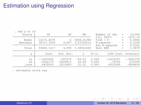
Estimation using Regression
. reg y x1 x2Source SS df MS Number of obs = 10,000
F(2, 9997) = 1571.70Model 12172.8278 2 6086.41388 Prob > F = 0.0000
Residual 38713.3039 9,997 3.87249214 R-squared = 0.2392Adj R-squared = 0.2391
Total 50886.1317 9,999 5.08912208 Root MSE = 1.9679
y Coef. Std. Err. t P>|t| [95% Conf. Interval]
x1 -.4187662 .007474 -56.03 0.000 -.4334167 -.4041156x2 .4382175 .0209813 20.89 0.000 .39709 .479345
_cons .4425514 .0210665 21.01 0.000 .4012569 .4838459
. estimates store reg
(StataCorp LP) October 20, 2016 Barcelona 31 / 59

Manual Two-Stage Least Squares (Wrong S.E.)
. quietly regress x1 z x2. predict double x1hat(option xb assumed; fitted values). preserve. replace x1 = x1hat(10,000 real changes made). quietly regress y x1 x2. estimates store manual. restore
(StataCorp LP) October 20, 2016 Barcelona 32 / 59

Estimation using Two-Stage Least Squares (2SLS)
. ivregress 2sls y x2 (x1=z)Instrumental variables (2SLS) regression Number of obs = 10,000
Wald chi2(2) = 1613.38Prob > chi2 = 0.0000R-squared = .Root MSE = 2.5174
y Coef. Std. Err. z P>|z| [95% Conf. Interval]
x1 -1.015205 .0252942 -40.14 0.000 -1.064781 -.9656292x2 1.005596 .0348808 28.83 0.000 .9372314 1.073961
_cons 1.042625 .0357962 29.13 0.000 .9724656 1.112784
Instrumented: x1Instruments: x2 z. estimates store tsls
(StataCorp LP) October 20, 2016 Barcelona 33 / 59

Estimation
. estimates table reg tsls manual, se
Variable reg tsls manual
x1 -.41876618 -1.0152049 -1.0152049.007474 .02529419 .02026373
x2 .4382175 1.0055965 1.0055965.02098126 .03488076 .02794373
_cons .44255137 1.0426249 1.0426249.02106646 .03579622 .02867713
legend: b/se
(StataCorp LP) October 20, 2016 Barcelona 34 / 59

Other Alternatives
sem, gsem, gmmThese are tools to construct our own estimationsem and gsem model the unobservable correlation in multipleequationsgmm is usually used to explicitly model a system of equationswhere we model the endogenous variable
(StataCorp LP) October 20, 2016 Barcelona 35 / 59

What are sem and gsem
SEM is for structural equation modeling and GSEM is forgeneralized structural equation modelingsem fits linear models for continuous responses. Models onlyallow for one level.gsem continuous, binary, ordinal, count, or multinomial, responsesand multilevel modeling.Estimation is done using maximum likelihoodIt allows unobserved components in the equations and correlationbetween equations
(StataCorp LP) October 20, 2016 Barcelona 36 / 59
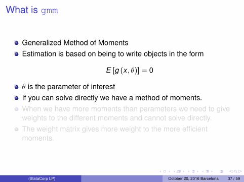
What is gmm
Generalized Method of MomentsEstimation is based on being to write objects in the form
E [g (x , θ)] = 0
θ is the parameter of interestIf you can solve directly we have a method of moments.When we have more moments than parameters we need to giveweights to the different moments and cannot solve directly.The weight matrix gives more weight to the more efficientmoments.
(StataCorp LP) October 20, 2016 Barcelona 37 / 59

Estimation Using sem
. sem (y <- x2 x1) (x1 <- x2 z), cov(e.y*e.x1) nologEndogenous variablesObserved: y x1Exogenous variablesObserved: x2 zStructural equation model Number of obs = 10,000Estimation method = mlLog likelihood = -71917.224
OIMCoef. Std. Err. z P>|z| [95% Conf. Interval]
Structuraly <-
x1 -1.015205 .0252942 -40.14 0.000 -1.064781 -.9656292x2 1.005596 .0348808 28.83 0.000 .9372314 1.073961
_cons 1.042625 .0357962 29.13 0.000 .9724656 1.112784
x1 <-x2 .9467476 .0244521 38.72 0.000 .8988225 .9946728z -.987925 .0241963 -40.83 0.000 -1.035349 -.9405011
_cons 1.011304 .0243764 41.49 0.000 .9635269 1.059081
var(e.y) 6.337463 .2275635 5.90678 6.799549var(e.x1) 5.941873 .0840308 5.779438 6.108874
cov(e.y,e.x1) 4.134763 .1675226 24.68 0.000 3.806424 4.463101
LR test of model vs. saturated: chi2(0) = 0.00, Prob > chi2 = .. estimates store sem
(StataCorp LP) October 20, 2016 Barcelona 38 / 59
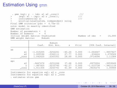
Estimation Using gmm
. gmm (eq1: y - {xb: x1 x2 _cons}) ///> (eq2: x1 - {xpi: x2 z _cons}), ///> instruments(x2 z) ///> winitial(unadjusted, independent) nologFinal GMM criterion Q(b) = 4.70e-33note: model is exactly identifiedGMM estimationNumber of parameters = 6Number of moments = 6Initial weight matrix: Unadjusted Number of obs = 10,000GMM weight matrix: Robust
RobustCoef. Std. Err. z P>|z| [95% Conf. Interval]
xbx1 -1.015205 .0252261 -40.24 0.000 -1.064647 -.9657627x2 1.005596 .0362111 27.77 0.000 .934624 1.076569
_cons 1.042625 .0363351 28.69 0.000 .9714094 1.11384
xpix2 .9467476 .0251266 37.68 0.000 .8975004 .9959949z -.987925 .0233745 -42.27 0.000 -1.033738 -.9421118
_cons 1.011304 .0243761 41.49 0.000 .9635274 1.05908
Instruments for equation eq1: x2 z _consInstruments for equation eq2: x2 z _cons. estimates store gmm
(StataCorp LP) October 20, 2016 Barcelona 39 / 59

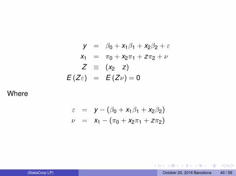
y = β0 + x1β1 + x2β2 + ε
x1 = π0 + x2π1 + zπ2 + ν
Z ≡ (x2 z)
E (Zε) = E (Zν) = 0
Where
ε = y − (β0 + x1β1 + x2β2)
ν = x1 − (π0 + x2π1 + zπ2)
(StataCorp LP) October 20, 2016 Barcelona 40 / 59
y = β0 + x1β1 + x2β2 + ε
x1 = π0 + x2π1 + zπ2 + ν
Z ≡ (x2 z)
E (Zε) = E (Zν) = 0
Where
ε = y − (β0 + x1β1 + x2β2)
ν = x1 − (π0 + x2π1 + zπ2)
(StataCorp LP) October 20, 2016 Barcelona 40 / 59

Summarizing the results of our estimation
. estimates table reg tsls sem gmm, eq(1) se ///> keep(#1:x1 #1:x2 #1:_cons)
Variable reg tsls sem gmm
x1 -.41876618 -1.0152049 -1.0152049 -1.0152049.007474 .02529419 .02529419 .02522609
x2 .4382175 1.0055965 1.0055965 1.0055965.02098126 .03488076 .03488076 .03621111
_cons .44255137 1.0426249 1.0426249 1.0426249.02106646 .03579622 .03579622 .03633511
legend: b/se
(StataCorp LP) October 20, 2016 Barcelona 41 / 59

Control Function Type Solutions
The key element here is to model the correlation between theunobservables between the endogenous variable equation andthe outcome equationThis is what is referred to as a control function approachHeckman selection is similar to this approach
(StataCorp LP) October 20, 2016 Barcelona 42 / 59

Heckman Selection
. clear. set seed 111. quietly set obs 20000.. // Generating Endogenous Components.. matrix C = (1, .4\ .4, 1). quietly drawnorm e v, corr (C).. // Generating exogenous variables.. generate x1 = rbeta(2 ,3). generate x2 = rbeta(2 ,3). generate x3 = rnormal(). generate x4 = rchi2(1).. // Generating outcome variables.. generate y1 = -1 - x1 - x2 + e. generate y2 = (1 + x3 - x4)*.5 + v. quietly replace y1 = . if y2 <=0. generate yp = y1 !=.
(StataCorp LP) October 20, 2016 Barcelona 43 / 59

Heckman Solution
Estimate a probit model for the selected observations as afunction of a set of variables ZThen use the probit models to estimate:
E (y |X1, y2 ≥ 0) = X1β + E (ε|X1, y2 ≥ 0)
= X1β + βsφ (Zγ)
Φ (Zγ)
In other words regress y on X1 and φ(Zγ)Φ(Zγ)
(StataCorp LP) October 20, 2016 Barcelona 44 / 59
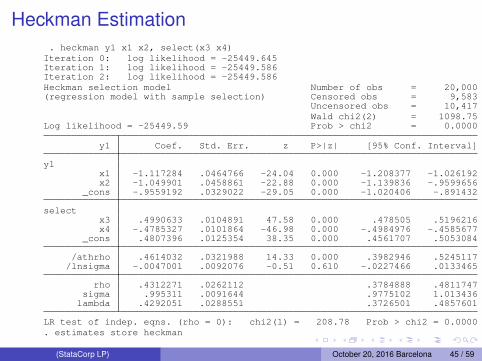
Heckman Estimation. heckman y1 x1 x2, select(x3 x4)
Iteration 0: log likelihood = -25449.645Iteration 1: log likelihood = -25449.586Iteration 2: log likelihood = -25449.586Heckman selection model Number of obs = 20,000(regression model with sample selection) Censored obs = 9,583
Uncensored obs = 10,417Wald chi2(2) = 1098.75
Log likelihood = -25449.59 Prob > chi2 = 0.0000
y1 Coef. Std. Err. z P>|z| [95% Conf. Interval]
y1x1 -1.117284 .0464766 -24.04 0.000 -1.208377 -1.026192x2 -1.049901 .0458861 -22.88 0.000 -1.139836 -.9599656
_cons -.9559192 .0329022 -29.05 0.000 -1.020406 -.891432
selectx3 .4990633 .0104891 47.58 0.000 .478505 .5196216x4 -.4785327 .0101864 -46.98 0.000 -.4984976 -.4585677
_cons .4807396 .0125354 38.35 0.000 .4561707 .5053084
/athrho .4614032 .0321988 14.33 0.000 .3982946 .5245117/lnsigma -.0047001 .0092076 -0.51 0.610 -.0227466 .0133465
rho .4312271 .0262112 .3784888 .4811747sigma .995311 .0091644 .9775102 1.013436
lambda .4292051 .0288551 .3726501 .4857601
LR test of indep. eqns. (rho = 0): chi2(1) = 208.78 Prob > chi2 = 0.0000. estimates store heckman
(StataCorp LP) October 20, 2016 Barcelona 45 / 59

Two Steps Heuristically
. quietly probit yp x3 x4. matrix A = e(b). quietly predict double xb, xb. quietly generate double mills = normalden(xb)/normal(xb). quietly regress y1 x1 x2 mills. matrix B = A, _b[x1], _b[x2], _b[_cons], _b[mills]
(StataCorp LP) October 20, 2016 Barcelona 46 / 59

GMM Estimation. local xb {b1}*x1 + {b2}*x2 + {b0b}
. local mills (normalden({xp:})/normal({xp:}))
. gmm (eq2: yp*(normalden({xp: x3 x4 _cons})/normal({xp:})) - ///> (1-yp)*(normalden(-{xp:})/normal(-{xp:}))) ///> (eq1: y1 - (`xb´) - {b3}*(`mills´)) ///> (eq3: (y1 - (`xb´) - {b3}*(`mills´))*`mills´), ///> instruments(eq1: x1 x2) ///> instruments(eq2: x3 x4) ///> winitial(unadjusted, independent) quickderivatives ///> nocommonesample from(B)Step 1Iteration 0: GMM criterion Q(b) = 2.279e-19Iteration 1: GMM criterion Q(b) = 2.802e-34Step 2Iteration 0: GMM criterion Q(b) = 5.387e-34Iteration 1: GMM criterion Q(b) = 5.387e-34note: model is exactly identifiedGMM estimationNumber of parameters = 7Number of moments = 7Initial weight matrix: Unadjusted Number of obs = *GMM weight matrix: Robust
RobustCoef. Std. Err. z P>|z| [95% Conf. Interval]
x3 .4992753 .0106148 47.04 0.000 .4784706 .52008x4 -.4779557 .0104455 -45.76 0.000 -.4984285 -.4574828
_cons .4798264 .012609 38.05 0.000 .4551132 .5045397
/b1 -1.115395 .0472637 -23.60 0.000 -1.20803 -1.02276/b2 -1.048694 .0455168 -23.04 0.000 -1.137905 -.9594823/b0b -.9514073 .0332245 -28.64 0.000 -1.016526 -.8862885/b3 .4199921 .0296825 14.15 0.000 .3618155 .4781686
* Number of observations for equation eq2: 20000Number of observations for equation eq1: 10417Number of observations for equation eq3: 10417
Instruments for equation eq2: x3 x4 _consInstruments for equation eq1: x1 x2 _consInstruments for equation eq3: _cons. estimates store heckgmm
(StataCorp LP) October 20, 2016 Barcelona 47 / 59

SEM Estimation of Heckman
. gsem (y1 <- x1 x2 L@a)(yp <- x3 x4 L@a, probit), ///> var(L@1) nologGeneralized structural equation model Number of obs = 20,000Response : y1 Number of obs = 10,417Family : GaussianLink : identityResponse : yp Number of obs = 20,000Family : BernoulliLink : probitLog likelihood = -25449.586( 1) - [y1]L + [yp]L = 0( 2) [var(L)]_cons = 1
Coef. Std. Err. z P>|z| [95% Conf. Interval]
y1 <-x1 -1.117284 .0464766 -24.04 0.000 -1.208377 -1.026192x2 -1.049901 .0458861 -22.88 0.000 -1.139836 -.9599656L .7287588 .0296352 24.59 0.000 .6706749 .7868426
_cons -.9559206 .0329017 -29.05 0.000 -1.020407 -.8914345
yp <-x3 .6175268 .0142797 43.24 0.000 .589539 .6455146x4 -.5921228 .0140871 -42.03 0.000 -.619733 -.5645125L .7287588 .0296352 24.59 0.000 .6706749 .7868426
_cons .5948535 .017244 34.50 0.000 .561056 .6286511
var(L) 1 (constrained)
var(e.y1) .4595557 .0322516 .4004984 .5273215
. estimates store hecksem
(StataCorp LP) October 20, 2016 Barcelona 48 / 59
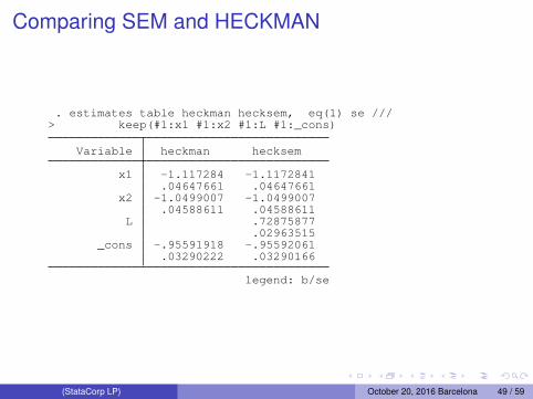
Comparing SEM and HECKMAN
. estimates table heckman hecksem, eq(1) se ///> keep(#1:x1 #1:x2 #1:L #1:_cons)
Variable heckman hecksem
x1 -1.117284 -1.1172841.04647661 .04647661
x2 -1.0499007 -1.0499007.04588611 .04588611
L .72875877.02963515
_cons -.95591918 -.95592061.03290222 .03290166
legend: b/se
(StataCorp LP) October 20, 2016 Barcelona 49 / 59

Non Built-In Situations
(StataCorp LP) October 20, 2016 Barcelona 50 / 59

Control Function Approach in a Linear Model: TheModel
. clear. set seed 111. set obs 10000number of observations (_N) was 0, now 10,000. generate a = rchi2(2). generate e = rchi2(1) -3 + a. generate v = rchi2(1) -3 + a. generate x2 = rnormal(). generate z = rnormal(). generate x1 = 1 - z + x2 + v. generate y = 1 - x1 + x2 + e
(StataCorp LP) October 20, 2016 Barcelona 51 / 59

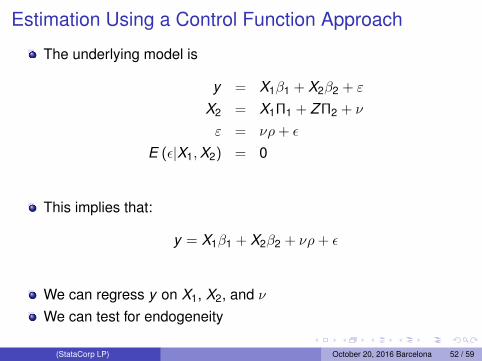
Estimation Using a Control Function Approach
The underlying model is
y = X1β1 + X2β2 + ε
X2 = X1Π1 + Z Π2 + ν
ε = νρ+ ε
E (ε|X1,X2) = 0
This implies that:
y = X1β1 + X2β2 + νρ+ ε
We can regress y on X1, X2, and νWe can test for endogeneity
(StataCorp LP) October 20, 2016 Barcelona 52 / 59

Estimation Using a Control Function Approach
The underlying model is
y = X1β1 + X2β2 + ε
X2 = X1Π1 + Z Π2 + ν
ε = νρ+ ε
E (ε|X1,X2) = 0
This implies that:
y = X1β1 + X2β2 + νρ+ ε
We can regress y on X1, X2, and νWe can test for endogeneity
(StataCorp LP) October 20, 2016 Barcelona 52 / 59
Estimation Using a Control Function Approach
The underlying model is
y = X1β1 + X2β2 + ε
X2 = X1Π1 + Z Π2 + ν
ε = νρ+ ε
E (ε|X1,X2) = 0
This implies that:
y = X1β1 + X2β2 + νρ+ ε
We can regress y on X1, X2, and νWe can test for endogeneity
(StataCorp LP) October 20, 2016 Barcelona 52 / 59

Estimation of Control Function Using gmm
. local xbeta {b1}*x1 + {b2}*x2 + {b3}*(x1-{xpi:}) + {b0}. gmm (eq3: (x1 - {xpi:x2 z _cons})) ///> (eq1: y - (`xbeta´)) ///> (eq2: (y - (`xbeta´))*(x1-{xpi:})), ///> instruments(eq3: x2 z) ///> instruments(eq1: x1 x2) ///> winitial(unadjusted, independent) nologFinal GMM criterion Q(b) = 1.45e-32note: model is exactly identifiedGMM estimationNumber of parameters = 7Number of moments = 7Initial weight matrix: Unadjusted Number of obs = 10,000GMM weight matrix: Robust
RobustCoef. Std. Err. z P>|z| [95% Conf. Interval]
x2 .9467476 .0251266 37.68 0.000 .8975004 .9959949z -.987925 .0233745 -42.27 0.000 -1.033738 -.9421118
_cons 1.011304 .0243761 41.49 0.000 .9635274 1.05908
/b1 -1.015205 .0252261 -40.24 0.000 -1.064647 -.9657627/b2 1.005596 .0362111 27.77 0.000 .934624 1.076569/b3 .6958685 .0284014 24.50 0.000 .6402028 .7515342/b0 1.042625 .0363351 28.69 0.000 .9714094 1.11384
Instruments for equation eq3: x2 z _consInstruments for equation eq1: x1 x2 _consInstruments for equation eq2: _cons
(StataCorp LP) October 20, 2016 Barcelona 53 / 59

Ordered Probit with Endogeneity
The model is given by:
y∗1 = y2β + xΠ + ε
y2 = xγ1 + zγ2 + ν
y1 = j if κj−1 < y∗1 < κj
κ0 = −∞ < κ1 < . . . < κk =∞ε ∼ N (0,1)
cov(ν, ε) 6= 0
(StataCorp LP) October 20, 2016 Barcelona 54 / 59

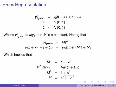
gsem Representation
y∗1gsem = y2b + xπ + t + Lαt ∼ N (0,1)
L ∼ N (0,1)
Where y∗1gsem = My∗1 and M is a constant. Noting that
y∗1gsem = My∗1y2b + xπ + t + Lα = y2Mβ + xMΠ + Mε
Which implies that
Mε = t + LαM2Var (ε) = Var (t + Lα)
M2 = 1 + α2
M =√
1 + α2
(StataCorp LP) October 20, 2016 Barcelona 55 / 59

Ordered Probit with Endogeneity: Simulation
. clear. set seed 111. set obs 10000number of observations (_N) was 0, now 10,000. forvalues i = 1/5 {
2. gen x`i´ = rnormal()3. }
.
. mat C = [1,.5 \ .5, 1]
. drawnorm e1 e2, cov(C)
.
. gen y2 = 0
. forvalues i = 1/5 {2. quietly replace y2 = y2 + x`i´3. }
. quietly replace y2 = y2 + e2
.
. gen y1star = y2 + x1 + x2 + e1
. gen xb1 = y2 + x1 + x2
.
. gen y1 = 4
.
. quietly replace y1 = 3 if xb1 + e1 <=.8
. quietly replace y1 = 2 if xb1 + e1 <=.3
. quietly replace y1 = 1 if xb1 + e1 <=-.3
. quietly replace y1 = 0 if xb1 + e1 <=-.8
(StataCorp LP) October 20, 2016 Barcelona 56 / 59

Ordered Probit with Endogeneity: Estimation. gsem (y1 <- y2 x1 x2 L@a, oprobit)(y2 <- x1 x2 x3 x4 x5 L@a), var(L@1) nolog
Generalized structural equation model Number of obs = 10,000Response : y1Family : ordinalLink : probitResponse : y2Family : GaussianLink : identityLog likelihood = -18948.444( 1) [y1]L - [y2]L = 0( 2) [var(L)]_cons = 1
Coef. Std. Err. z P>|z| [95% Conf. Interval]
y1 <-y2 1.284182 .0217063 59.16 0.000 1.241638 1.326725x1 1.28408 .0290087 44.27 0.000 1.227224 1.340936x2 1.293582 .0287252 45.03 0.000 1.237282 1.349883L .7968852 .0155321 51.31 0.000 .7664428 .8273275
y2 <-x1 .9959898 .0099305 100.30 0.000 .9765263 1.015453x2 1.002053 .0099196 101.02 0.000 .9826106 1.021495x3 .9938048 .0096164 103.34 0.000 .974957 1.012653x4 .9984898 .0095031 105.07 0.000 .9798642 1.017115x5 1.002206 .0095257 105.21 0.000 .9835358 1.020876L .7968852 .0155321 51.31 0.000 .7664428 .8273275
_cons .0089433 .0099196 0.90 0.367 -.0104987 .0283853
y1/cut1 -1.017707 .0291495 -34.91 0.000 -1.074839 -.9605751/cut2 -.4071202 .0273925 -14.86 0.000 -.4608085 -.3534319/cut3 .4094317 .0275357 14.87 0.000 .3554628 .4634006/cut4 1.017637 .029513 34.48 0.000 .9597921 1.075481
var(L) 1 (constrained)
var(e.y2) .348641 .0231272 .3061354 .3970482
(StataCorp LP) October 20, 2016 Barcelona 57 / 59

Ordered Probit with Endogeneity: Transformation
. nlcom _b[y1:y2]/sqrt(1 + _b[y1:L]^2)_nl_1: _b[y1:y2]/sqrt(1 + _b[y1:L]^2)
Coef. Std. Err. z P>|z| [95% Conf. Interval]
_nl_1 1.004302 .0189557 52.98 0.000 .9671491 1.041454
. nlcom _b[y1:x1]/sqrt(1 + _b[y1:L]^2)_nl_1: _b[y1:x1]/sqrt(1 + _b[y1:L]^2)
Coef. Std. Err. z P>|z| [95% Conf. Interval]
_nl_1 1.004222 .0214961 46.72 0.000 .9620909 1.046354
. nlcom _b[y1:x2]/sqrt(1 + _b[y1:L]^2)_nl_1: _b[y1:x2]/sqrt(1 + _b[y1:L]^2)
Coef. Std. Err. z P>|z| [95% Conf. Interval]
_nl_1 1.011654 .0213625 47.36 0.000 .9697838 1.053523
(StataCorp LP) October 20, 2016 Barcelona 58 / 59

Conclusion
We established a general framework for endogeneity where theproblem is that the unobservables are related to observablesWe saw solutions using instrumental variables or modeling thecorrelation between unobservablesWe saw how to use gmm and gsem to estimate this models both inthe cases of existing Stata commands and situations not availablein Stata
(StataCorp LP) October 20, 2016 Barcelona 59 / 59