dear author, please note that changes made in the online ... · 19 the earliest proponents of...

Dear author,

Please note that changes made in the online proofing system will be added to the article before publication but are not reflected in this PDF.

We also ask that this file not be used for submitting corrections.

ARTICLE IN PRESS

JID: YREEC [m3Gsc; June 23, 2017;14:6 ]

Research in Economics xxx (2017) xxx–xxx

Contents lists available at ScienceDirect

Research in Economics

journal homepage: www.elsevier.com/locate/rie

Nominal GDP targeting for developing countries

Pranjul Bhandari , Jeffrey Frankel ∗Q1

Harvard Kennedy School, Harvard University, 79 JFK St., Cambridge, MA 02138, United States

a r t i c l e i n f o

Article history:

Received 5 May 2017

Accepted 1 June 2017

Available online xxx

Keywords:

Central bank

Developing

Emerging markets

GDP

Income

India

Inflation

IT

Monetary policy

Monsoon

Nominal

Shock

Supply

Target

Terms of trade

a b s t r a c t

Interest in nominal GDP (NGDP) targeting has come in the context of large advanced

economies. Developing countries are better suited for it, however, in light of big supply

shocks and terms of trade shocks, such as monsoon rains and oil import price shocks in

the case of India. Under annual inflation targeting (IT), the full impact of adverse supply

shocks is felt as lost real GDP. NGDP targeting automatically accommodates such shocks,

while retaining the advantage of anchoring expectations. We derive the condition under

which NGDP targeting would dominate other regimes such as annual IT, to achieve objec-

tives of output and price stability. We estimate key parameters for the case of India and

conclude that the condition may indeed hold.

© 2017 University of Venice. Published by Elsevier Ltd. All rights reserved.

India’s central bank has contemplated a move from its multi-indicator monetary policy approach, towards a simple 1

credibility-enhancing nominal rule. It seems to favor a flexible inflation target, which it hopes will help lower inflation 2

expectations that have been high and sticky since 2010. 1 3

In the paper we evaluate nominal GDP (NGDP) as an alternative monetary policy target for a country like India, especially 4

in the face of the large supply shocks that it faces. 2 We outline a simple model to compare NGDP targeting with other 5

nominal rules. We find that under certain simplifying assumptions and plausible conditions, setting an annual NGDP target 6

may indeed dominate Inflation targeting (IT), which is here defined as an setting an annual target for the inflation rate. 7

The paper is organized as follows. Section 1 discusses the origins and resurgence of NGDP targeting. The proposal has 8

surfaced several times in the last few decades – though not always as a solution to the same problem – suggesting its all- 9

weather-friend characteristics. Section 2 highlights a simple theoretical model that compares alternative nominal monetary 10

policy rules in terms of their ability to minimize a quadratic loss function capturing the objectives of price stability and 11

output stability. We show the conditions necessary for one regime to dominate the other. Section 3 discusses the evolution 12

∗ Corresponding author.

E-mail address: [email protected] (J. Frankel). 1 RBI (2014), Jha (2008) and Mohan and Kapur (2009) see drawbacks to inflation targeting for India. 2 Ranging from high growth and low inflation in 20 03–20 06 to high growth and high inflation in 2010–11 to low growth and high inflation in the

2011–2014 period.

http://dx.doi.org/10.1016/j.rie.2017.06.001

1090-9443/© 2017 University of Venice. Published by Elsevier Ltd. All rights reserved.

Please cite this article as: P. Bhandari, J. Frankel, Nominal GDP targeting for developing countries, Research in Economics

(2017), http://dx.doi.org/10.1016/j.rie.2017.06.001


http://www.ScienceDirect.com

http://www.elsevier.com/locate/rie

mailto:[email protected]



2 P. Bhandari, J. Frankel / Research in Economics xxx (2017) xxx–xxx

ARTICLE IN PRESS


of monetary policy in India since independence in 1947 and the central bank’s desire to adopt a nominal rule. Section 4 visits 13

the different supply side shocks to which the country seems susceptible. Section 5 empirically tests the conditions outlined 14

in Section 2 to ascertain if indeed NGDP targeting would minimize the quadratic loss function for the case of India. We 15

use two-stage-least-squares to estimate the parameters of the supply curve. Section 6 addresses some practical concerns in 16

implementing a NGDP rule, particularly the problem of revisions in the nominal GDP statistics. Section 8 concludes. 17

1. Origins and resurgence of NGDP targeting and relevance for developing countries 18

The earliest proponents of nominal GDP targeting were Meade (1978) and Tobin (1980) , followed by other economists in 19

the 1980s. The historical context was a desire to earn credibility for monetary discipline and lower inflation rates. 20

The early 1980s saw monetarism as the official policy regime in some major countries. It was soon frustrated, however by 21

an unstable money demand function. NGDP targeting was designed specifically to counter such velocity shocks. Nevertheless 22

it was not adopted anywhere. The concept was on the backburner for several decades. Instead, the dominant approach for 23

many smaller and developing countries between the mid-1980s and mid-1990s was a return to exchange rate targets. 24

A series of speculative attacks in the late 1990s forced many countries to abandon exchange rate anchors and move to 25

some form of floating exchange rates. Mid-sized countries may anyway want to have a floating exchange rate in order to 26

accommodate terms of trade shocks and other real shocks. But if the exchange rate is not to be the anchor for monetary 27

policy, what is? 28

The 20 0 0s saw the spread of IT, Inflation Targeting, from some advanced economies to many emerging market countries. 29

Over the last two decades, it is believed to have contributed to bringing down inflation across many countries and to have 30

anchored expectations. The Global Financial Crisis (GFC) of 2008–09 provoked possible concerns over shortcomings of IT, 31

analogous perhaps to the frustrations with exchange rate targets that had resulted from the currency crises of the 1990s. 32

Criticisms of Inflation Targeting include its narrow focus, lack of attention to asset market bubbles, failure to hit announced 33

targets, and mistaken tightening in response to supply shocks such as the mid-2008 oil price spike. 34

Interest in NGDP targeting revived, now as an alternative to inflation targeting. 3 But it has been focused on advanced 35

economies such as the US, UK, Japan and Euroland, where interest rates have been constrained by the “zero lower bound.”36

The motive for NGDP targeting in this literature is to achieve a credible monetary expansion and higher inflation rates, which 37

are quite the opposite of the context that Meade (1978) and Tobin (1980) had in mind. This flexibility of NGDP targeting, as 38

a practical way to achieve the goal of the day, be it monetary easing or tightening, and its focus on stabilizing demand are 39

longstanding advantages. 40

Attention to developing and middle income countries in the NGDP targeting literature is scant. 4 And yet they may be the 41

ones who can benefit the most from an NGDP target. 42

Developing countries have some characteristics that differ from advanced countries when it comes to setting monetary 43

policy. 5 First, many developing countries have more acute need of monetary policy credibility. Some are newly born with an 44

absence of well-established institutions, some have recently moved to a new monetary policy setting, some have a checkered 45

past with central banks accommodating government debt, and some have had periods of hyperinflation. 46

The need for credibility amplifies the desirability of choosing a nominal target that the central bank does not keep 47

missing repeatedly. Central banks should choose targets ex ante that they will be willing to live with ex post and that they 48

have relatively higher ability to achieve. For instance, announcing a strict inflation target that is then repeatedly missed 49

would tend to erode credibility. One study showed that IT central banks in emerging market countries miss declared targets 50

by more than do industrialized countries ( Fraga et al., 2003 ). 6 51

Second, developing and middle income countries tend to be more exposed to terms of trade shocks, because they are 52

more likely to export commodities and to be price takers on world markets, and to supply shocks, because of the importance 53

of agriculture, social instability and productivity changes. Productivity shocks are likely to be larger in developing countries: 54

during a boom, the country does not know in real time whether rapid growth is a permanent increase in productivity 55

growth (it is the next Asian tiger) or temporary (the result of a transitory fluctuation in commodity markets or domestic 56

demand). 7 57

Weather disasters and terms of trade shocks are particularly useful from an econometric viewpoint, because these supply 58

shocks are both measureable and exogenous. As Fig. 2 below shows, they tend to be bigger in emerging markets and low- 59

income countries than in advanced economies. 60

The choice of target variable depends on the type of shock to which the country is susceptible. We will see that, the 61

more common are supply shocks, the more appropriate is NGDP targeting. It splits the effects between inflation and GDP 62

growth rather than suffering adverse supply shocks in the form of lost GDP alone. 63

3 E.g. Woodford’s (2012) theoretical analysis, Hatzius’ (2011) market viewpoint, and Scott Sumner’s blog posts. 4 The few studies available include Frankel (1995b), McKibbin and Singh (2003) , and Frankel et al. (2008) for East Asia, India and South Africa respectively. 5 A survey of the literature is available in Frankel (2011) . 6 In part this may be because central banks in developing countries have a harder time hitting any target than in advanced economies: the mone-

tary transmission mechanism usually works poorly due to oligopolistic banks and undeveloped financial markets. Mishra and Montiel (2012) . For India:

Aleem (2010) and Mohanty (2012) . 7 The trend growth rate in emerging market countries is highly variable and uncertain: Aguiar and Gopinath (2007) .




P. Bhandari, J. Frankel / Research in Economics xxx (2017) xxx–xxx 3

ARTICLE IN PRESS


Fig. 1. Elevated inflation expectations in India.

Fig. 2. Emerging markets and low income countries are more susceptible to supply shocks

Source: IMF, 2011 .

Three categories of supply or trade shocks are relevant in particular: 64

a. Pure supply shock – Natural disasters (such as an earthquake, hurricane, cyclone, tidal wave, or flood), other weather- 65

related events (drought or severe winter), social disruption (labor strike or social unrest), and other productivity shocks 66

(technological progress) fall under this category. For India, a poor monsoon is a good example. A fixed exchange rate by 67

definition prevents the currency from depreciating and thereby moderating the fall in the trade balance and GDP. A CPI 68

target, if interpreted literally, implies that monetary policy must be tightened enough to choke off any increase in the 69

price level, leading again to lower GDP growth. Only in case of NGDP targeting can the currency respond to an adverse 70

supply or terms of trade shocks by depreciating, helping the trade balance and splitting the adverse impact of the shock 71

between inflation and growth. 72

b. Rise in import price. One form of terms of trade shock is an increase in the world price of importable goods. For India, 73

oil prices are a good example. In the case of an exchange rate target, by definition the currency is prevented from 74

depreciating, with adverse implications for the trade balance and GDP. In the case of CPI targeting, if interpreted literally, 75

the currency must actually appreciate to prevent a rise in CPI inflation, with even worse implications for the trade 76

balance and growth. In case of NGDP targeting, by contrast, the currency is not led to appreciate. Again the adverse 77

shock is split between inflation and GDP growth rather than growth alone. 78

c. Fall in export price. Many developing countries export commodities that undergo large price swings on world markets. In 79

the case of exchange rate targeting the currency cannot adjust. In the case of CPI targeting, depreciation is also limited as 80





ARTICLE IN PRESS


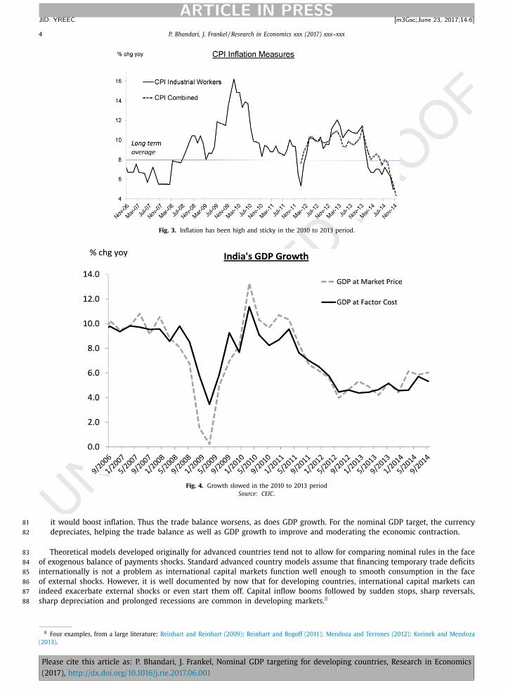
Fig. 3. Inflation has been high and sticky in the 2010 to 2013 period.

Fig. 4. Growth slowed in the 2010 to 2013 period

Source: CEIC .

it would boost inflation. Thus the trade balance worsens, as does GDP growth. For the nominal GDP target, the currency 81

depreciates, helping the trade balance as well as GDP growth to improve and moderating the economic contraction. 82

Theoretical models developed originally for advanced countries tend not to allow for comparing nominal rules in the face 83

of exogenous balance of payments shocks. Standard advanced country models assume that financing temporary trade deficits 84

internationally is not a problem as international capital markets function well enough to smooth consumption in the face 85

of external shocks. However, it is well documented by now that for developing countries, international capital markets can 86

indeed exacerbate external shocks or even start them off. Capital inflow booms followed by sudden stops, sharp reversals, 87

sharp depreciation and prolonged recessions are common in developing markets. 8 88

8 Four examples, from a large literature: Reinhart and Reinhart (2009); Reinhart and Rogoff (2011); Mendoza and Terrones (2012); Korinek and Mendoza

(2013) .





ARTICLE IN PRESS


NGDP targeting could potentially bring in some of the same benefits of discretion while yet keeping inflation expectations 89

anchored. In the model below, we formalize this intuition and probe further the circumstances under which NGDP targets 90

would dominate the alternatives. 91

2. Theoretical underpinnings: comparing discretion with four alternative nominal rules 92

It is well established that a credible nominal target can eliminate an inflationary bias that discretion otherwise allows in 93

a Barro and Gordon (1983) type model of dynamic inconsistency. But it makes a difference what is the choice of nominal 94

target, because the economy is vulnerable to short run shocks ( Rogoff, 1985; Fischer, 1990 ). The ex post impact of the shocks 95

depends on the variable chosen ex ante to be the nominal target. 96

Using a simple model outlined by Frankel (1995a,b ), 9 we compare four alternative nominal policy rules in the con- 97

duct of monetary policy: full discretion by the central banker, money supply rule, price level rule and nominal GDP rule, 98

respectively. 10 99

Our investigation of these policy rules is predicated on the argument that one wants to announce some simple variable 100

to which the central bank will commit. Credible commitment to a nominal target, for example, is a means of defeating 101

the inflation bias from Barro–Gordon dynamic inconsistency. Our mathematical derivation will focus on the case where the 102

point of committing to a target is to reduce expected inflation, because this case remains relevant for India and many other 103

developing countries. The desire for transparency and accurate communication is not limited, however, to the Barro–Gordon 104

argument for credible commitment to disinflation. It includes also the recent arguments for credible commitment to higher 105

inflation. It is not even limited to a choice among alternative nominal anchors like inflation, the exchange rate or M1; the 106

desire to offer forward guidance has included announcements of other intermediate variables such as the unemployment 107

rate. 108

Inflation targeting and NGDP targeting can be formulated in terms of either levels or rates of change. A possible advan- 109

tage of targeting a level is a faster return to the goal. If the regime is credible, an incipient shortfall in the NGDP level (or 110

price level) engenders expectations of a subsequent monetary expansion and higher inflation, thus automatically contribut- 111

ing to lower real interest rates and an accelerated move towards the goal. 11 The disadvantage of targeting a level is that 112

the public may not fully understand, comprehend or believe a target in levels as it would a target in growth rates. For our 113

model, the distinction between levels and growth may not be important. Targets are set each year; announcing it in levels 114

or growth would amount to the same thing. 115

While we show derivations for a number of different nominal rules here, our main interest is in comparing two of them: 116

CPI inflation targeting versus NGDP targeting. The former is the rule the Reserve Bank of India (RBI) is considering and the 117

latter is the alternative on which we focus. 118

To simplify the analysis, we assume rigid rules in our theoretical analysis, keeping in mind that welfare ranking for rigid 119

rules in theory might be different than that for flexible rules ( Rogoff, 1985 ). 120

The aggregate supply relationship is assumed throughout to be: 121

y = y + b

(p − p

e )

+ u , (1)

where y is real output, y is potential output, p is the price index, p

e is the expected price index (variables can be in log 122

levels or annual growth rate), and u is a supply disturbance. 123

We assume objectives captured by the simple quadratic loss function: 124

L = a p

2 +

(y − ˆ y

)2 , (2)

where a is the weight assigned to the inflation objective and ˆ y is the desired level of output. 125

In order to build an expansionary bias to discretionary policy making, the ˆ y > y condition is imposed, as in Barro and 126

Gordon (1983) . For simplicity we have assumed that the preferred level of inflation is zero. It could as easily be 2% or any 127

other number. Substituting (1) into (2) , 128

L = a p

2 +

[y − ˆ y + b

(p − p

e )

+ u

]2 . (3)

2.1. Discretionary policy 129

Under full discretion, the policy maker chooses aggregate demand so as to minimize the loss function every period. 130

Taking the derivative and setting it equal to zero, dL/dp = 0, gives: 131

p =

[−b

(y − ˆ y

)+ b

2 p

e − bu

]/ [a + b

2 ]. (4)

9 An inflation target for an open economy, which was not covered in Frankel (1995a,b ), is also derived here. 10 A fifth regime, exchange rate targeting, was also considered in an earlier version of this paper, NBER Working Paper No. 20898. 11 Indeed that is the Woodford (2012) argument for targeting the level of NGDP level, in advanced economies constrained by a zero-lower-bound on

interest rates.





ARTICLE IN PRESS


Under rational expectations, 132

p

e = Ep =

(ˆ y − y

)b / a . (5)

This term reflects the inflationary bias that Barro and Gordon (1983) attribute to discretion. Central banks have to inflate 133

just to keep up with expectations, even without achieving higher output. The aim of a credible nominal target is to remove 134

this inflationary bias. However, the economy will still be vulnerable to short run shocks, the impact of which will depend 135

on the variable it chooses as the nominal target ( Rogoff, 1985; Fischer, 1990 ). 136

Combining (5) and (4) gives the solution for ex post inflation under discretion: 137

p =

(ˆ y − y

)[ b / a ] − ub /

[a + b

2 ]. (6)

Combining (6) and (2) gives the value of the expected loss function: 138

EL =

(1 + b

2 / a )(

y − ˆ y )2 +

[a /

(a + b

2 )]

var ( u ) (7)

The first term represents the inflationary bias while the second represents the impact of supply disturbances after au- 139

thorities have chosen the optimal split between inflation and output. 140

2.2. Money rule 141

The money market equilibrium condition is given as–142

m = p + y − v , (8)

where v represents velocity shocks. We assume that v is uncorrelated with u. If authorities pre-commit to a money growth 143

rule to reduce expected inflation in the long run equilibrium, they must give up on affecting y. The optimal money growth 144

rate is the one that sets Ep = 0 12 ; thus setting money supply, m, at Ey, which in this case is y. The aggregate demand 145

equation thus becomes: 146

p + y = y + v . (9)

We combine (9) with (1) to solve: 147

y = y + ( u + bv ) / ( 1 + b ) , p = ( v − u ) / ( 1 + b ) . (10)

Substituting into (2) gives, 148

EL =

(y − ˆ y

)2 +

{( 1 + a ) var ( u ) +

(a + b

2 )var ( v )

}/ ( 1 + b )

2 (11)

The first term is smaller than the corresponding term in the discretion case, because pre-commitment eliminates ex- 149

pected inflation. But the second term could likely be larger, as the authorities give up the ability to respond to money 150

demand shocks. Which regime is better, depends on the size of the shocks and the value of a, i.e., the weight placed on 151

price stability. 152

2.3. Nominal GDP rule 153

In the case of a nominal GDP rule, authorities vary money supply in such a way that velocity shocks are accommodated 154

and p + y in Eq. (9) is constant. The solution is the same as in the money rule but with the v disturbance dropped out. Thus 155

the loss function is reduced to: 156

EL =

(y − ˆ y

)2 +

[( 1 + a ) / ( 1 + b )

2 ]

var ( u ) . (12)

This unambiguously dominates the money rule (11) , so long as there are any velocity shocks. 157

It is not possible to know whether the rule dominates discretion unless the values of the parameters such as var(u) and 158

a are known. Although the first term (reflecting inflationary bias) is smaller for the nominal GDP rule, the second term 159

depends on the value of the parameters (which we investigate later in the paper). 160

2.4. Inflation rule 161

Under Inflation Targeting, the authorities set monetary policy so that the price index (level or rate) is zero, not just in 162

expectation but also in the face of ex post shocks. From (3) this gives 163

L =

[(y − ˆ y

)+ u

]2 (13)

164

EL =

(y − ˆ y

)2 + var ( u ) . (14)

12 We assume for simplicity that desired inflation is zero.





ARTICLE IN PRESS


Comparison shows that the price level rule dominates the money supply rule if velocity shocks are large. If they are 165

small, the money supply rule collapses to the nominal GDP rule. 166

The nominal GDP rule dominates the price rule if supply shocks u are important and if –167 [( 1 + a ) / ( 1 + b )

2 ]

< 1 , i . e ., so long as a / b < 2 + b .

The conclusion is that NGDP targeting dominates IT except in the absence of supply shocks, the presence of a very steep 168

supply curve and/or a very high weight on the price stability objective in the quadratic loss function. 169

The condition can be simplified further if one is willing to infer an estimate a , the weight on price stability, from the 170

Taylor Rule. The original Taylor Rule, which is still widely used, gives equal weights to output and price stability in setting 171

its real interest rate policy instrument, implying a = 1. In that case the condition a/b < 2 + b collapses to b >

√

2 – 1 . This 172

implies that for the nominal GDP rule to dominate the price rule, the AS curve must be flat enough that its slope ( 1/b ) is 173

less than 2.414. 174

We re-cap the key condition, which depends on magnitudes of parameters that will be revisited in a later section: 175

For nominal GDP targeting to dominate price or inflation targeting, the condition is a < (2 + b)b . For a = 1, as in the 176

original Taylor rule, this inequality boils down to a flat AS curve: 1/b < 2.414. 177

Having discussed the theoretical underpinnings, we will need some parameter estimates to ascertain whether the con- 178

dition for NGDP targeting dominating IT is likely to hold for the case of India. We first discuss the evolution of monetary 179

policy making in India before evaluating its suitability to a NGDP target. 180

3. Evolution of monetary policy making in India 181

3.1. Brief history 182

India’s monetary policy framework has undergone several significant transformations. Starting with an exchange rate 183

anchor after independence in 1947, it moved to the use of credit aggregates as the nominal anchor in 1957. Changes in the 184

Bank rate and Cash Reserve Ratio were the main policy instruments supporting its credit allocation functions and ‘social 185

control’ over channeling credit to ‘priority sectors’ ( RBI, 2014 ). 186

Monetization of fiscal deficit, its inflationary consequence and crowding out of private sector credit called for a change 187

in the monetary regime, leading to a new era of monetary targeting in 1985. Broad money was the intermediate target 188

and reserve money was the main operating instrument. However this policy framework was fraught with problems. Un- 189

constrained credit to the government fuelled inflation. Capital flows following the 1991 liberalization further eroded control 190

over monetary aggregates. Meanwhile, structural reforms in the 1990s led to a shift in financing patterns for the govern- 191

ment. Gradually, interest rates and the exchange rate started to become more market determined and the RBI was able to 192

move from direct to more indirect market based instruments. 193

In 1998, the RBI moved to a ‘multiple indicators approach’, whereby it considered many variables – growth, inflation, ex- 194

change rates, credit growth, capital flows, fiscal position, trade, etc. This approach worked for the next decade, with inflation 195

rate (WPI and CPI-IW) falling from 8–9% to 5–6% over the ten years. 13 196

3.2. Call for a new approach 197

The period 2010 to mid-2014, however, raised questions on the efficacy of the multiple indicators approach. Inflation was 198

high and sticky and growth had fallen substantially for an extended period of time. Several commentators questioned the 199

effectiveness of the approach, calling for a well-defined nominal target which would provide clarity with respect to what 200

the RBI should do. 201

The RBI governor set up a committee of experts to recommend the way forward. The committee in its January 2014 202

report recommended a “flexible inflation target” for the conduct of monetary policy with the combined CPI inflation as 203

nominal anchor, set at 4% with a + / − 2% band. 14 204

The report noted that India has one of the highest inflation rates amongst G-20 countries and that elevated inflation was 205

creating macroeconomic vulnerabilities. (High inflation distinguishes those countries that were most hit by the rise in US 206

interest rates in the “taper tantrum” of May-June 2013. 15 ) The report emphasized that “high inflation itself becomes a risk 207

to growth” and “limits the space for accommodating growth concerns”16 implying that the current situation of stagflation 208

would benefit from enhanced price stability. 209

It stated, “Stabilizing and anchoring inflation expectations – whether they are rational or adaptive – is critical for ensuring 210

price stability on an enduring basis, so that monetary policy re-establishes credibility visibly and transparently, that deviations 211

from desirable levels of inflation on a persistent basis will not be tolerated.”212

13 E.g., Mohan (2009) and Mohan and Patra (2009) , Hutchison et al. (2013) find that Indian monetary policy has alternated between periods of focus on

controlling inflation and periods when more weight is given to output and the exchange rate. 14 It also laid out a transition path: “The transition path to the target zone should be graduated to bringing down inflation from the current level of 10% to

8% over a period not exceeding the next 12 months and to 6% over a period not exceeding the next 24 month period before formally adopting the recommended

target of 4% inflation with a band of + / −2% ”. On the problem of getting inflation expectations and inflation down in India, see Patra and Ray (2010) . 15 Klemm et al. (2014) . 16 Referring to Friedman (1977), Fischer (1993) and Barro (1995).





ARTICLE IN PRESS


Fig. 5. India experiences terms-of-trade shocks like other Emerging Market countries

Source: World Bank, WDI .

4. Vulnerability to supply shocks 213

We saw in Section 2 that assessing the ability of NGDP targeting to minimize the quadratic loss function requires us to 214

know if supply shocks are important. Before moving on to evaluate for the case of India the other key criterion, involving 215

the slope of the supply relationship, we discuss the supply shocks to which the country is prone. 216

In the January 2014 RBI report referred to in the previous section, the central bank explicitly acknowledged “the vul- 217

nerability of the Indian economy to supply/external shocks …” and its impact on monetary policy. As argued above, nominal 218

GDP targeting is more likely to dominate alternative rules when a country is vulnerable to supply shocks. Furthermore, we 219

need exogenous and measureable supply shocks if we are to identify movements along the aggregate demand curve. The 220

productivity shocks beloved of advanced-country macro models probably will not meet these criteria. 221

India imports much of the oil and gas it consumes. It has recently also begun to import coal for fuelling its electricity 222

plants. Thus it is susceptible to changes in global prices of fossil fuels. The World Bank’s index for the net barter terms of 223

trade shows India as typical of emerging markets in the high volatility of its terms of trade ( Fig. 5 ). 224

India over the last few decades has faced natural disasters ranging from earthquakes and tsunamis, to super-cyclones 225

and floods, often causing huge disruptions. It also suffers chronically from annual uncertainty regarding rains during the 226

monsoon season. Data show that these rains have an important bearing on inflation and growth nationally, and not merely 227

regionally. No doubt productivity shocks are also important in India as well, but they are neither as easily measured nor as 228

clearly exogenous as weather events and terms of trade shocks. 229

The estimated aggregate demand relationship will incorporate whatever reaction function the monetary authorities fol- 230

low during the sample period. If they target m , we are estimating Eq. (8) . If they target inflation, then the weather and 231

oil shocks should in theory show no effect on the price index. If they are already targeting nominal GDP, even if only im- 232

plicitly, then the weather and oil shocks should have equiproportionate effects on output (negative) and the price level 233

(positive). 234

5. Estimating India’s aggregate supply curve 235

To undertake an evaluation of NGDP targeting versus inflation targeting, one must know a few key parameters, particu- 236

larly the slope of the AS curve (see Section II.A.4). In principle, these parameters can be estimated, so long as we have good 237

instrumental variables to identify the two equations. Our structure of equations for deriving these estimates is related to 238

seminal work on estimating the New Keynesian Philips Curve ( Roberts, 1995 ). The system of equations can be estimated in 239

a 2SLS framework, equivalent to Instrumental Variables. 240





ARTICLE IN PRESS


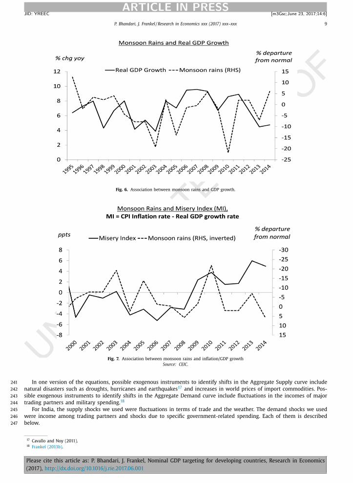
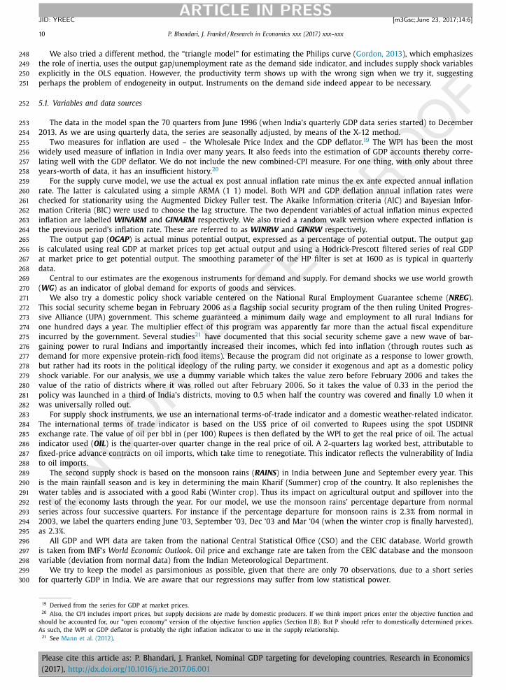
Fig. 6. Association between monsoon rains and GDP growth.

Fig. 7. Association between monsoon rains and inflation/GDP growth

Source: CEIC .

In one version of the equations, possible exogenous instruments to identify shifts in the Aggregate Supply curve include 241

natural disasters such as droughts, hurricanes and earthquakes 17 and increases in world prices of import commodities. Pos- 242

sible exogenous instruments to identify shifts in the Aggregate Demand curve include fluctuations in the incomes of major 243

trading partners and military spending. 18 244

For India, the supply shocks we used were fluctuations in terms of trade and the weather. The demand shocks we used 245

were income among trading partners and shocks due to specific government-related spending. Each of them is described 246

below. 247

17 Cavallo and Noy (2011). 18 Frankel (2013b) .





ARTICLE IN PRESS


We also tried a different method, the “triangle model” for estimating the Philips curve ( Gordon, 2013 ), which emphasizes 248

the role of inertia, uses the output gap/unemployment rate as the demand side indicator, and includes supply shock variables 249

explicitly in the OLS equation. However, the productivity term shows up with the wrong sign when we try it, suggesting 250

perhaps the problem of endogeneity in output. Instruments on the demand side indeed appear to be necessary. 251

5.1. Variables and data sources 252

The data in the model span the 70 quarters from June 1996 (when India’s quarterly GDP data series started) to December 253

2013. As we are using quarterly data, the series are seasonally adjusted, by means of the X-12 method. 254

Two measures for inflation are used – the Wholesale Price Index and the GDP deflator. 19 The WPI has been the most 255

widely used measure of inflation in India over many years. It also feeds into the estimation of GDP accounts thereby corre- 256

lating well with the GDP deflator. We do not include the new combined-CPI measure. For one thing, with only about three 257

years-worth of data, it has an insufficient history. 20 258

For the supply curve model, we use the actual ex post annual inflation rate minus the ex ante expected annual inflation 259

rate. The latter is calculated using a simple ARMA (1 1) model. Both WPI and GDP deflation annual inflation rates were 260

checked for stationarity using the Augmented Dickey Fuller test. The Akaike Information criteria (AIC) and Bayesian Infor- 261

mation Criteria (BIC) were used to choose the lag structure. The two dependent variables of actual inflation minus expected 262

inflation are labelled WINARM and GINARM respectively. We also tried a random walk version where expected inflation is 263

the previous period’s inflation rate. These are referred to as WINRW and GINRW respectively. 264

The output gap ( OGAP ) is actual minus potential output, expressed as a percentage of potential output. The output gap 265

is calculated using real GDP at market prices top get actual output and using a Hodrick-Prescott filtered series of real GDP 266

at market price to get potential output. The smoothing parameter of the HP filter is set at 1600 as is typical in quarterly 267

data. 268

Central to our estimates are the exogenous instruments for demand and supply. For demand shocks we use world growth 269

( WG ) as an indicator of global demand for exports of goods and services. 270

We also try a domestic policy shock variable centered on the National Rural Employment Guarantee scheme ( NREG ). 271

This social security scheme began in February 2006 as a flagship social security program of the then ruling United Progres- 272

sive Alliance (UPA) government. This scheme guaranteed a minimum daily wage and employment to all rural Indians for 273

one hundred days a year. The multiplier effect of this program was apparently far more than the actual fiscal expenditure 274

incurred by the government. Several studies 21 have documented that this social security scheme gave a new wave of bar- 275

gaining power to rural Indians and importantly increased their incomes, which fed into inflation (through routes such as 276

demand for more expensive protein-rich food items). Because the program did not originate as a response to lower growth, 277

but rather had its roots in the political ideology of the ruling party, we consider it exogenous and apt as a domestic policy 278

shock variable. For our analysis, we use a dummy variable which takes the value zero before February 2006 and takes the 279

value of the ratio of districts where it was rolled out after February 2006. So it takes the value of 0.33 in the period the 280

policy was launched in a third of India’s districts, moving to 0.5 when half the country was covered and finally 1.0 when it 281

was universally rolled out. 282

For supply shock instruments, we use an international terms-of-trade indicator and a domestic weather-related indicator. 283

The international terms of trade indicator is based on the US$ price of oil converted to Rupees using the spot USDINR 284

exchange rate. The value of oil per bbl in (per 100) Rupees is then deflated by the WPI to get the real price of oil. The actual 285

indicator used ( OIL ) is the quarter-over quarter change in the real price of oil. A 2-quarters lag worked best, attributable to 286

fixed-price advance contracts on oil imports, which take time to renegotiate. This indicator reflects the vulnerability of India 287

to oil imports. 288

The second supply shock is based on the monsoon rains ( RAINS ) in India between June and September every year. This 289

is the main rainfall season and is key in determining the main Kharif (Summer) crop of the country. It also replenishes the 290

water tables and is associated with a good Rabi (Winter crop). Thus its impact on agricultural output and spillover into the 291

rest of the economy lasts through the year. For our model, we use the monsoon rains’ percentage departure from normal 292

series across four successive quarters. For instance if the percentage departure for monsoon rains is 2.3% from normal in 293

2003, we label the quarters ending June ’03, September ’03, Dec ’03 and Mar ’04 (when the winter crop is finally harvested), 294

as 2.3%. 295

All GDP and WPI data are taken from the national Central Statistical Office (CSO) and the CEIC database. World growth 296

is taken from IMF’s World Economic Outlook . Oil price and exchange rate are taken from the CEIC database and the monsoon 297

variable (deviation from normal data) from the Indian Meteorological Department. 298

We try to keep the model as parsimonious as possible, given that there are only 70 observations, due to a short series 299

for quarterly GDP in India. We are aware that our regressions may suffer from low statistical power. 300

19 Derived from the series for GDP at market prices. 20 Also, the CPI includes import prices, but supply decisions are made by domestic producers. If we think import prices enter the objective function and

should be accounted for, our "open economy" version of the objective function applies (Section II.B). But P should refer to domestically determined prices.

As such, the WPI or GDP deflator is probably the right inflation indicator to use in the supply relationship. 21 See Mann et al. (2012) .





ARTICLE IN PRESS


Table 1

Estimation of supply relationship

First stage dependent variable: output gap

Second stage (Inverted supply equation) dependent variable: inflation surprises (winarm/ginarm/ginrw).

P 1 2 3 4

Variables Output gap

First-stage regressions

World GDP 0 .541 ∗∗∗ 0 .495 ∗∗∗ 0 .558 ∗∗∗ 0 .561 ∗∗∗

(0 .109) (0 .107) (0 .109) (0 .109)

NREG 0 .006 a 0 .006 ∗ 0 .007 ∗

(0 .004) (0 .004) (0 .004)

Constant −0 .019 ∗∗∗ −0 .015 ∗∗∗ −0 .020 ∗∗∗ −0 .020 ∗∗∗

(0 .005) (0 .004) (0 .004) (0 .005)

R 2 0 .396 0 .371 0 .422 0 .416

Prob > F 0 .0 0 0 0 .0 0 0 0 .0 0 0 0 .0 0 0

Variables Inflation Surprises

Second-stage regressions WInfl arm WInfl arm GInfl arm GInfl RW

Output gap 0 .666 ∗∗∗ 0 .562 ∗∗∗ 0 .384 ∗∗ 0 .533 ∗∗

(0 .203) (0 .202) (0 .182) (0 .265)

Oil ( −2) 0 .093 ∗ 0 .096 ∗ 0 .074 b 0 .138 ∗

(0 .053) (0 .05) (0 .049) (0 .071)

Rains −0 .065 ∗∗ −0 .057 ∗∗ −0 .041 ∗ −0 .081 ∗∗

(0 .026) (0 .025) (0 .024) (0 .034)

Constant −0 .003 −0 .002 −0 .002 −0 .003

(0 .002) (0 .002) (0 .002) (0 .003)

Observations 70 70 65 66

(Standard errors in parentheses.) ∗∗∗ p < 0.01, ∗∗ p < 0.05, ∗p < 0.1, a p = 0.11, b p = 0.135

Note: First stage non-instrument variables are not shown in the table.

Memo: List of variables with brief description

WInf arm and GInf arm: Annual inflation rate minus expected inflation rate derived from an ARMA

model for WPI and GDP deflator respectively

GInfl RW: Annual GDP deflator inflation rate minus expected inflation rate derived from a random walk

assumption

Output Gap: Output gap based on GDP data with potential calculated by passing through the HP filter

Aggregate demand instruments:

World GDP: World annual GDP growth

NREG: Dummy variable taking the value of zero when the National Rural Employment Guarantee had

not started and the value of ratio of districts covered when it was operating

Aggregate supply shocks:

Oil ( −2): This terms of trade variable is calculated as US$ price of a barrel of oil times the USDINR

exchange rate, to get the Rupee value of oil. This is then deflated by WPI inflation index to convert to

real terms. The series used is the quarterly change in the real value of oil. A two quarter lag worked

best.

Rains: Percentage deviation of monsoon rains from normal. The data-point for each year’s monsoon rain

(e.g. 2003) are applied for four consecutive quarters (ending June ’03, Sep ’03, Dec ’03 and Mar ’04)

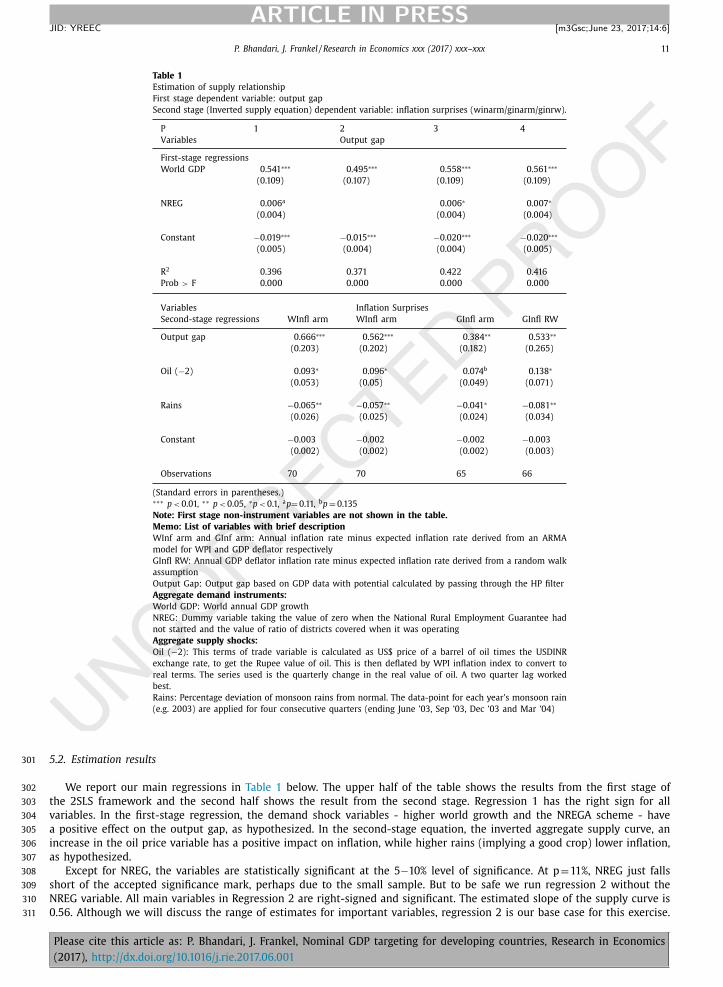
5.2. Estimation results 301

We report our main regressions in Table 1 below. The upper half of the table shows the results from the first stage of 302

the 2SLS framework and the second half shows the result from the second stage. Regression 1 has the right sign for all 303

variables. In the first-stage regression, the demand shock variables - higher world growth and the NREGA scheme - have 304

a positive effect on the output gap, as hypothesized. In the second-stage equation, the inverted aggregate supply curve, an 305

increase in the oil price variable has a positive impact on inflation, while higher rains (implying a good crop) lower inflation, 306

as hypothesized. 307

Except for NREG, the variables are statistically significant at the 5 −10% level of significance. At p = 11%, NREG just falls 308

short of the accepted significance mark, perhaps due to the small sample. But to be safe we run regression 2 without the 309

NREG variable. All main variables in Regression 2 are right-signed and significant. The estimated slope of the supply curve is 310

0.56. Although we will discuss the range of estimates for important variables, regression 2 is our base case for this exercise. 311





ARTICLE IN PRESS


Table 2

NGDP targeting dominates discretion and inflation targeting in

a closed economy setting.

Base case (based on regression 2)

Parameter and variable values

a 1 .00

b 1 .78

1/b 0 .56

Var(u) 0 .0 0 02

k > 1

y ∗ > 0

Implications:

NGDP targeting dominates discretionary policy.

NGDP targeting dominates price targeting.

In general, given that we have more observations with a WPI based regression, we prefer it over the GDP-deflator based 312

regression. 313

In regression 3, we use the GDP deflator instead of WPI. All variables are right signed, though OIL is now only significant 314

at the 14% level. Again, this could be due to lack of statistical power in the dataset. The slope of the AS curve is 0.38 under 315

this specification. In regression 4, we try the random walk assumption for inflation expectations. We find an estimated AS 316

curve slope of 0.53. 317

We also tried another set of regressions using lagged output gap as an additional instrument for output gap. Instrument- 318

ing with lagged values is a common empirical strategy in the New Keynesian Phillips Curve literature. The reasoning is that 319

if expectations are rational, the rational expectations forecast error must be uncorrelated with past information (Gali and 320

Gertler, 1999). In this vein, if one thinks that variables influencing inflation are mostly news shocks that are uncorrelated 321

with past information, then instrumenting with lagged variables makes perfect sense. (In fact, it’s the only thing that makes 322

sense, because news shocks will presumably be correlated with most contemporaneous variables). But if one isn’t willing to 323

assume that the omitted variables are news shocks, then lagged variables may fail the exclusion restriction. 324

This contentious issue is beyond the scope of this paper. But we have tried it both ways, running regression 2 along with 325

lagged output gap as an instrument for the output gap. All variables have the right sign and are significant at the 5% level 326

of significance. The estimated slope of the supply curve is 0.34, which is a dash lower than some of the results in Table 1 . 327

5.3. Implications of the supply slope estimate 328

The estimated short run aggregate supply curve slope ( 1/b ) ranges from 0.4 to 0.6. It is statistically significant at the 95% 329

to 99% confidence level (1 to 5% significance level). This is broadly in line with other research. Patra and Kapur (2010) point 330

to an AS curve slope in the 0.3 to 0.6 range for India over a one-year horizon. 331

Recall that the necessary condition for nominal GDP targeting to minimize the quadratic loss function, if a = 1, is 332

1/b < 2.414 (Section II.A). This condition is easily met: all four estimates are at least seven standard errors below 2.4. 333

Some later versions of the Taylor Rule (Taylor 1999) assign a smaller weight of a = 0.5 to inflation. This would make 334

the condition a < (2 + b)b that was derived in Section II.A.iv easier to satisfy; a sufficient condition would be an AS slope 335

less than 10. Thus there are grounds for believing that NGDP targets accommodate supply shocks better than does Inflation 336

Targeting. 337

The parameters also allow us to test if nominal rules dominate discretionary policy in the context of the Barro–Gordon–338

Rogoff model. 22 Table 2 with our base case assumptions suggests that NGDP targeting indeed may dominate, not just over 339

inflation targeting, but over discretionary policy as well. When we use a range of estimates, for instance include estimates 340

of b and var(u) as per the other (non-base case) regressions we have run, we continue to get the same outcome: NGDP 341

targeting minimizes the quadratic loss function. 342

6. Practical application of the NGDP targeting rule 343

Several issues and arguments have been raised as to why it might not be practical to target NGDP. We discuss some of 344

the main concerns and discuss what it would mean operationally in India. 345

An occasional misunderstanding arises when it is presumed that a single number for the NGDP growth target would be 346

set for all time. This is not the proposal. Rather the target would be set regularly, perhaps annually. A variety of factors 347

would lead to different growth targets over time: long run revisions in the estimated rate of growth of potential output, 348

aspirations to bring the steady-state rate of inflation gradually down over time, a temporary desire for either enhanced 349

22 Although India does not admit to having a discretionary policy, the rather opaque multi indicator approach could be interpreted as essentially discre-

tionary policy making.





ARTICLE IN PRESS


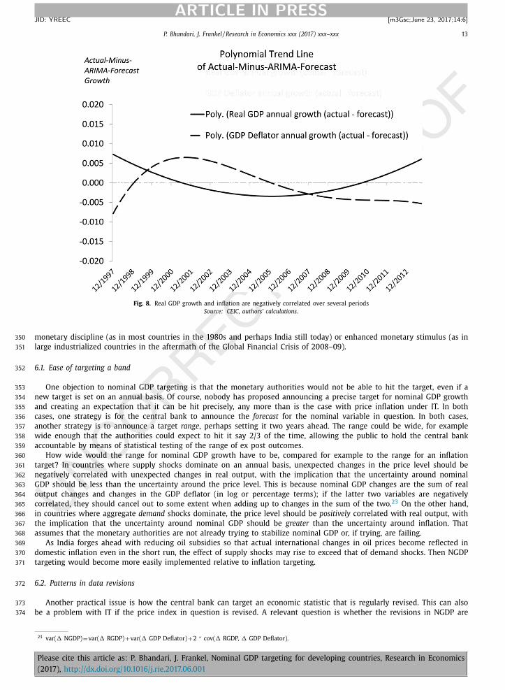
Fig. 8. Real GDP growth and inflation are negatively correlated over several periods

Source: CEIC, authors’ calculations .

monetary discipline (as in most countries in the 1980s and perhaps India still today) or enhanced monetary stimulus (as in 350

large industrialized countries in the aftermath of the Global Financial Crisis of 2008 –09). 351

6.1. Ease of targeting a band 352

One objection to nominal GDP targeting is that the monetary authorities would not be able to hit the target, even if a 353

new target is set on an annual basis. Of course, nobody has proposed announcing a precise target for nominal GDP growth 354

and creating an expectation that it can be hit precisely, any more than is the case with price inflation under IT. In both 355

cases, one strategy is for the central bank to announce the forecast for the nominal variable in question. In both cases, 356

another strategy is to announce a target range , perhaps setting it two years ahead. The range could be wide, for example 357

wide enough that the authorities could expect to hit it say 2/3 of the time, allowing the public to hold the central bank 358

accountable by means of statistical testing of the range of ex post outcomes. 359

How wide would the range for nominal GDP growth have to be, compared for example to the range for an inflation 360

target? In countries where supply shocks dominate on an annual basis, unexpected changes in the price level should be 361

negatively correlated with unexpected changes in real output, with the implication that the uncertainty around nominal 362

GDP should be less than the uncertainty around the price level. This is because nominal GDP changes are the sum of real 363

output changes and changes in the GDP deflator (in log or percentage terms); if the latter two variables are negatively 364

correlated, they should cancel out to some extent when adding up to changes in the sum of the two. 23 On the other hand, 365

in countries where aggregate demand shocks dominate, the price level should be positively correlated with real output, with 366

the implication that the uncertainty around nominal GDP should be greater than the uncertainty around inflation. That 367

assumes that the monetary authorities are not already trying to stabilize nominal GDP or, if trying, are failing. 368

As India forges ahead with reducing oil subsidies so that actual international changes in oil prices become reflected in 369

domestic inflation even in the short run, the effect of supply shocks may rise to exceed that of demand shocks. Then NGDP 370

targeting would become more easily implemented relative to inflation targeting. 371

6.2. Patterns in data revisions 372

Another practical issue is how the central bank can target an economic statistic that is regularly revised. This can also 373

be a problem with IT if the price index in question is revised. A relevant question is whether the revisions in NGDP are 374

23 var( � NGDP) = var( � RGDP) + var( � GDP Deflator) + 2 ∗ cov( � RGDP, � GDP Deflator).





ARTICLE IN PRESS


greater than or smaller than the revisions in prices. To answer this, we start by comparing the change between first and 375

final estimate for both nominal GDP and the deflator. 376

Data on this are limited as the Central Statistical Organization in India only began issuing a press release with real- 377

time quarterly GDP data from March 2007. All quarterly data prior to then were released in one block and there was no 378

distinction between first and final estimate. A regular press release is necessary to make a series of first estimates which 379

can be compared to the final estimate. We have 20 observations for which both the first and the final estimate are available. 380

Using these data we find that on average, the absolute change between the first and final estimate of nominal GDP was 381

0.7% while that in GDP deflator was a slightly higher 0.8%. The variance of the revisions in nominal GDP was 1.7, while that 382

in the GDP deflator was slightly higher at 1.8. This suggests that hitting the nominal GDP target may not be any harder than 383

hitting the GDP deflator target, when considering revisions in data. 384

However, revisions in the combined Consumer Price Index data (which the RBI has suggested as the inflation index to 385

target if inflation targeting is to be employed), are small compared to revisions in the GDP deflator, and could therefore have 386

implementation advantages over both GDP deflator targeting and nominal GDP targeting. 387

So the difficulty in targeting precisely might work out to be a drawback to NGDP targeting relative to CPI inflation 388

targeting. But just because CPI inflation is not prone to revisions, does not necessarily mean that it is a more accurate 389

indicator of price movements than the GDP deflator. Most importantly, on a conceptual level, getting close to the tar- 390

get is not necessarily an advantage if it is the wrong target. CPI inflation gives the wrong policy response for terms of 391

trade shocks. The ideal response to a fall in the export price is currency depreciation, mitigating the fall in the trade 392

balance and output. CPI targeting constrains depreciation because it would otherwise raise import prices which enter the 393

CPI. 24 394

6.3. A rule like nominal GDP targeting may already characterize India’s monetary policy 395

In their 2012 paper, RBI staff members Michael Patra and Muneesh Kapoor show that a hybrid McCallum Taylor Rule 396

(where policy interest rates react to deviations of nominal income growth from its time varying trend growth rate) is 397

strongly supported by data in explaining the conduct of Indian monetary policy. The rule that they find superior to all 398

is a forward looking Taylor rule with the effective policy interest rate reacting to inflation and two period ahead output gap. 399

The McCallum Taylor Rule is akin to the NGDP targeting that we propose, suggesting that it may already be a part of 400

India’s policy setting and could be formalized with relative ease and bringing home the advantages of both a rule and 401

discretion. As Bean (2013) has argued, NGDP targeting may be a way to bring greater transparency and credibility to what 402

the central bank is doing anyway. 403

7. Operationalizing NGDP targeting in India … in baby steps 404

The Reserve Bank of India has declared its determination to bring down the high inflation rates experienced in recent 405

years . A common interpretation of Inflation Targeting is to set a single unchanging goal for inflation in the long term, such 406

as 2%. Our conception of NGDP targeting is completely consistent with keeping this language for long-run inflation. 25 At 407

stake is only the question of what annual targets are set in the near term. 408

The RBI could ease gradually into setting annual NGDP targets. The first step would be reporting NGDP forecasts in its 409

quarterly Macroeconomic and Monetary Developments document which comes along with the quarterly policy statement. 410

This could be an easy addition given that the document already carries real GDP and inflation forecasts. 26 Over time, it 411

might increasingly emphasize discussion of the future path of NGDP. Such discussion would likely be less vulnerable to 412

future shocks than are the projections for the inflation rate (or for real GDP), to the extent that the supply shocks or trade 413

shocks render the latter out of date. Even under a complete transition to formal NGDP targets, the central bank could 414

continue to indicate its best guesses as to the annual levels of inflation and real growth that would correspond. But the 415

fundamental point is that, in the event of a supply or trade shock, the authorities could remind everyone that the nominal 416

GDP target is the one to which it is committed, not CPI inflation. 417

For practical feasibility it is better if NGDP data are relatively reliable and not susceptible to revisions as large as those 418

that now regularly occur. While some revision is normal (and done globally), to the extent the Central Statistical Organiza- 419

tion can improve and update its data collection mechanism, NGDP targeting would be more successful. 420

India has data peculiarities, for instance divergence between the different measures of inflation and between GDP in 421

market prices and at factor costs. A good understanding of these episodes of divergence will be helpful before embarking on 422

any nominal targeting regime. Finally, our model is a simple and intuitive framework. More sophisticated analysis, keeping 423

in mind the peculiarities in emerging markets vis-à-vis advanced countries, would be useful. Q2 424

24 Frankel (2012) . 25 Frankel (2013a) . 26 One will have to be careful, however, to distinguish GDP at factor cost vs. market price. Market price estimates are likely to be more appropriate here.





ARTICLE IN PRESS


8. Conclusion 425

We have seen, in Section 3 , that supply shocks are important for India. Section 5 then yielded parameter estimates that 426

satisfied the other key condition derived in Section 2 . The implication seems to be that annual NGDP targeting offers a 427

smaller value of the quadratic loss function than does annual inflation targeting. Q3 428

NGDP targets automatically break down the pain from adverse supply shocks between lower growth and higher infla- 429

tion, rather than suffering lower growth alone. It is versatile enough to address varying macroeconomic episodes, from 430

circumstances calling for disinflation (as in advanced countries in the 1980s and many developing countries still today) to 431

circumstances calling for monetary stimulus (as in the aftermath of a big negative demand shock), to circumstances calling 432

for holding the course steady. It can automatically bring about a desired policy response to situations varying from high 433

inflation and low growth (akin to India’s macroeconomic situation in 2011 –13) to low inflation and high growth (a possi- 434

ble outcome of productivity enhancing structural reforms). In the former, it will avoid an excessively tight monetary policy 435

response and in the latter it will avoid an excessively loose policy response. Q4 436

Uncited references Q5

437

Frankel, 2004, International Monetary Fund 2011, ISI Emerging Markets 2017, Patra and Kapur, 2012, Rafiq, 2011, Ramcha- 438

ran, 2007, Broda, 2004, Céspedes and Velasco, 2012, Christensen, 2013, Edwards and Yeyati, 2005, Fischer, 1977 . 439

References 440

Aguiar, M., Gopinath, G., 2007. Emerging market business cycles: the cycle is the trend. J. Polit. Econ. (115) 69–102. 441 Aleem, A., 2010. Transmission mechanism of monetary policy in india. J. Asian Econ. 21 (2), 186–197. 442 Barro, R., Gordon, D., 1983. A positive theory of monetary policy in a natural rate model. J. Polit. Econ. 91 (4), 589–610. 443 Bean, C., 2013. Nominal income targets: an old wine in a new bottle. Bank of England Deputy Governor’s speech at the Institute for Economic Affairs 4 4 4

Conference on the State of the Economy, London, Feb. 27. 445 Broda, C., 2004. Terms of trade and exchange rate regimes in developing countries. J. Int. Econ. 63 (1), 31–58. 446 Céspedes, L.F., Velasco, A., 2012. Macroeconomic performance during commodity price booms and busts. IMF Econ. Rev. 60, 570–599 December NBER 447

Working Paper No 18569 (Cambridge, Massachusetts, National Bureau of Economic Research). 448 Christensen, L., 2013. In India, inflation is everywhere and always a rainy phenomenon. Market Monetarist Jan. 24. 449 Edwards, S., Yeyati, E.L., 2005. Flexible exchange rates as shock absorbers. Eur. Econ. Rev. 49 (8) November 2079–005. 450 Fischer, S., 1977. Stability and exchange rate systems in a monetarist model of the balance of payments. In: Aliber, R. (Ed.), The Political Economy of 451

Monetary Reform. Osmun and Co. Publ., NY: Allanheld, pp. 59–73. 452 Fischer, S., 1990. Rules versus discretion in monetary policy. In: Friedman, B.M., Hahn, F.H. (Eds.). In: Handbook of Monetary Economics, 2. Elsevier, Ams- 453

terdam, pp. 1155–1184. chapter 21. 454 Fraga, A., Goldfajn, I., Minella, A., 2003. Inflation targeting in emerging market economies. NBER Working Paper 10019, October. National Bureau of Economic 455

Research, Cambridge, Massachusetts. 456 Frankel, J., 1995a. The stabilizing properties of a nominal GNP rule. J. Money Credit Banking 27 (2) May. 457 Frankel, J., 1995b. Monetary regime choices for a semi-open country. In: Edwards, S. (Ed.), Capital Controls, Exchange Rates and Monetary Policy in the 458

World Economy. Cambridge University Press, Cambridge, UK. 459 Frankel, J., 2004. Experience of and lessons from exchange rate regimes in emerging economies. In: Monetary and Financial Integration in East Asia: The 460

Way Ahead, Asian Development Bank. Palgrave Macmillan, pp. 91–138. 461 Frankel, J., 2011. Monetary policy in emerging markets: a survey. In: Friedman, B., Woodford, M. (Eds.), Handbook of Monetary Economics. Elsevier, Amster- 462

dam. 463 Frankel, J., 2012. Product price targeting – a new improved way of inflation targeting. MAS Monet. Rev. XI (1), 2–5 April (Monetary Authority of Singapore). 464 Frankel, J., 2013a. Nominal-GDP targets, without losing the inflation anchor. In: Reichlin, L., Baldwin, R. (Eds.), Is Inflation Targeting Dead: Central Banking 465

After the Crisis. CEPR, London, pp. 90–94. 466 Frankel, J., 2013b. Exchange Rate and Monetary Policy For Kazakhstan in Light of Resource Exports. Harvard University December. 467 Frankel, J., Smit, B., Sturzenegger, F., 2008. Fiscal and monetary policy in a commodity based economy. Econ. Transition 16 (4), 679–713 Oct. 468 Gordon, R.J., 2013. The Philips curve is alive and well: inflation and the NAIRU during the slow recovery. NBER Working Paper No. 19390. National Bureau 469

of Economic Research, Cambridge, Massachusetts August. 470 Hatzius, J., 2011. The case for a nominal GDP level target. US Economics Analyst. Goldman Sachs Global ECS Research October. 471 Hutchison, M., Sengupta, R., Singh, N., 2013. Dove or hawk? Characterizing monetary policy regime switches in India. Emerging Markets Rev. 16, 183–202. 472 International Monetary Fund, 2011. Managing volatility: a vulnerability exercise for low-income countries. Prepared By the Strategy, Policy, and Review, 473

Fiscal Affairs, and Research Departments in Consultation With Area Departments March. 474 ISI Emerging Markets: CEIC database 2017. 475 Jha, R., 2008. Inflation targeting in India: issues and prospects. Int. Rev. Appl. Econ. 22 (2), 259–270. 476 Klemm, A., Meier, A., Sosa, S., 2014. Taper Tantrum or Tedium: How U.S. Interest Rates Affect Financial Markets in Emerging Economies. International 477

Monetary Fund, Washington, DC May 22. 478 Korinek, A., Mendoza, E., 2013. From Sudden stops to fisherian deflation: quantitative theory and policy implications. NBER Working Paper No. 19362. 479

National Bureau of Economic Research, Cambridge, Massachusetts August. 480 McKibbin, W.J. and Singh, K., 2003: “Issues in the choice of a monetary regime for India”, Brookings Discussion Paper in International Economics, No. 154, 481

September. 482 Mendoza, E.G., Terrones, M.E., 2012. An anatomy of credit booms and their demise. NBER Working Paper 18379. National Bureau of Economic Research, 483

Cambridge, Massachusetts September. 484 Mann, N., Pande, V. and Shah, M., 2012, “MGNREGA sameeksha: an anthology of research studies on the Mahatma Gandhi national rural employment 485

guarantee act, 2005 ′′ . 486 Mishra, P., Montiel, P., 2012. How Effective is monetary transmission in low-income countries? A survey of the empirical evidence. IMF Working Paper 487

12/143. International Monetary Fund, Washington, DC. 488 Mohan, R., 2009. Capital account liberalization and conduct of monetary policy: the Indian experience. Macroecon. Finance Emerg. Market Econ. 2 (2), 489

215–238. 490 Mohan, R., and Kapur, M., 2009, “Managing the impossible trinity: volatile capital flows and Indian monetary policy,” Available at SSRN 1861724. 491 Mohan, R., Patra, M., 2009. Monetary policy transmission in India. In: Hammond, G., Ravi Kanbur, S.M., Prasad, E. (Eds.), Monetary Policy Frameworks For 492

Emerging Markets, p. 153. 493





ARTICLE IN PRESS


Mohanty, D., 2012. Evidence of interest rate channel of monetary policy transmission in India. RBI Working Paper Series, 6/2012. Reserve Bank of India, 494 Mumbai. 495

Patra, M.D., Kapur, M., 2012. Alternative monetary policy rules for India. IMF Working Paper. International Monetary Fund, Washington, DC April. 496 Patra, M.D., Kapur, M., 2010. A monetary policy model without money for India. IMF Working Paper. International Monetary Fund, Washington, DC August. 497 Patra, M.D., Ray, P., 2010. Inflation Expectations and Monetary Policy in India: An Empirical Exploration International Monetary Fund Working Paper 10/84. 498 Rafiq, M.S., 2011. Sources of economic fluctuations in oil-exporting economies: implications for choice of exchange rate regimes. Int. J. Econ. Finance 16 (1), 499

70–91 Jan. 500 Ramcharan, R., 2007. Does the exchange rate regime matter for real shocks? Evidence from windstorms and earthquakes. J. Int. Econ. 73 (1), 31–47. 501 Reinhart, C., Reinhart, V., 2009. Capital flow bonanzas: an encompassing view of the past and present. In: Frankel, J., Pissarides, C. (Eds.), NBER International 502

Seminar On Macroeconomics 2008. University of Chicago Press, Chicago. 503 Reinhart, C., Rogoff, K., 2011. This Time is Different. Princeton University Press, Princeton. 504 Reserve Bank of India, 2014, “Report of the expert committee to revise and strengthen the monetary policy framework“, January. 505 Roberts, J.M., 1995. New keynesian economics and the Philips curve. J. Money Credit Banking 27 Part 1, November. 506 Rogoff, K., 1985. The optimal degree of commitment to an intermediate monetary target. Q. J. Econ. 1169–1189 November. 507 Tobin, J., 1980. Stabilization policy ten years after. Brookings Papers Econ. Activity (1) 19–72. 508 Woodford, M., 2012. Policy methods of accommodation at the interest-rate lower bound. Presented at the Jackson Hole Symposium. Federal Reserve Bank 509

of Kansas City August. 510




dear author, please note that changes made in the online ... · 19 the earliest proponents of...

Documents