Debt Redemption and Reserve Accumulation

Laura Alfaro Fabio Kanczuk

Working Paper 13-074

Working Paper 13-074

Copyright © 2017 by Laura Alfaro and Fabio Kanczuk

Working papers are in draft form. This working paper is distributed for purposes of comment and discussion only. It may not be reproduced without permission of the copyright holder. Copies of working papers are available from the author.

Debt Redemption and Reserve Accumulation

Laura Alfaro Harvard Business School

Fabio Kanczuk Ministry of Finance, Brazil

Debt Redemption and Reserve Accumulation*

Laura Alfaro Harvard Business School and NBER

Fabio Kanczuk Ministry of Finance, Brazil

August 2017

Abstract

In the past decade, foreign participation in local-currency bond markets in emerging countries increased dramatically. We revisit sovereign debt sustainability under the assumptions that countries can accumulate reserves and borrow internationally using their own currency. As opposed to traditional sovereign-debt models, asset-valuation effects occasioned by currency fluctuations act to absorb global shocks and render consumption smoother. Countries do not accumulate reserves to be depleted in “bad” times. Instead, issuing domestic debt while accumulating reserves acts as a hedge against external shocks. A quantitative exercise of the Brazilian economy suggests this strategy to be effective for smoothing consumption and reducing the occurrence of default.

JEL classification: F34 Key words: Sovereign Debt, Local-Currency Bonds, Foreign Reserves.

* lalfaro@hbs.edu. Harvard Business School, Boston, MA 02163, Tel: 617-495-7981, Fax: 617-495-5985; kanczuk@usp.br. Department of Economics, Universidade de São Paulo, and Secretary of Economic Policy, Ministry of Finance, Brazil. The paper does not reflect the views of the Brazilian Ministry of Finance. We thank for their valuable comments and suggestions Nan Li, two anonymous referees, Enrique Alberola-Ila, Javier Bianchi, Roberto Chang, Menzie Chinn, Charles Engel, Jeffrey Frankel, Marcio Garcia, Galina Hale, Ricardo Hausmann, Lakshmi Iyer, Carmen Reinhart, Jesse Schreger, Eric Werker, and participants in seminars at the Kennedy School of Government, Harvard Business School, Fundacão Getulio Vargas, University of São Paulo, University of Wisconsin-Madison, and participants at the LACEA, and the Brazilian Central Bank Inflation Targeting Conference. Hayley Pallan and Haviland Sheldahl-Thomason provided great research assistance. Support from Harvard Business School research budget acknowledged.

2

1 Introduction

The past decade has seen the impressive development of domestic government bond

markets in emerging market economies (EMEs). Market depth increased, maturities

lengthened, and the investor base broadened as a consequence of active foreign participation

in local-currency bond markets. At the same time, EMEs accumulated international reserves.

However, since the interest earned from international reserves is much lower than that paid

on EMEs’ debts, this policy seems puzzling. What is the role of international reserves if these

countries have the option of inflating away domestic debt and face no significant external

liquidity risks? Why are these reserves not used to repay debt? Are international reserves

ultimately increasing or decreasing the sustainability of EMEs’ debt?

This paper revisits the question about the optimal level of debt and foreign reserves

under novel assumptions that reflect the recent developments of capital flows to emerging

markets. In particular, increased foreign participation in local-currency bond markets implies

that emerging countries borrow internationally in domestic-currency-denominated bonds.

This makes them subject to new sets of constraints regarding repayment of their liabilities,

and exposes them to new incentives to actively accumulate international reserves.

Two trends characterize capital flows and portfolio holdings of emerging countries

over the past decade. The first is a strong increase in foreign participation in local-currency

bond markets in emerging economies. Using a newly constructed dataset of the currency

composition of sovereign and corporate external debt, Du and Schreger (2015a, b) show that

over the past decade major emerging market sovereigns that borrowed as much as 85% of

their external debt in foreign currency now borrow more than half in their own currency.

Figure 1 displays the increase in domestic-currency denominated debt in a sample of

emerging markets.

3

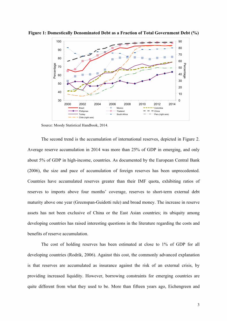
Figure 1: Domestically Denominated Debt as a Fraction of Total Government Debt (%)

Source: Moody Statistical Handbook, 2014.

The second trend is the accumulation of international reserves, depicted in Figure 2.

Average reserve accumulation in 2014 was more than 25% of GDP in emerging, and only

about 5% of GDP in high-income, countries. As documented by the European Central Bank

(2006), the size and pace of accumulation of foreign reserves has been unprecedented.

Countries have accumulated reserves greater than their IMF quota, exhibiting ratios of

reserves to imports above four months’ coverage, reserves to short-term external debt

maturity above one year (Greenspan-Guidotti rule) and broad money. The increase in reserve

assets has not been exclusive of China or the East Asian countries; its ubiquity among

developing countries has raised interesting questions in the literature regarding the costs and

benefits of reserve accumulation.

The cost of holding reserves has been estimated at close to 1% of GDP for all

developing countries (Rodrik, 2006). Against this cost, the commonly advanced explanation

is that reserves are accumulated as insurance against the risk of an external crisis, by

providing increased liquidity. However, borrowing constraints for emerging countries are

quite different from what they used to be. More than fifteen years ago, Eichengreen and

0

10

20

30

40

50

60

70

80

90

30

40

50

60

70

80

90

100

2000 2002 2004 2006 2008 2010 2012 2014

Percentage P

erce

ntag

e

Brazil Mexico Colombia Phillipines Thailand China Turkey South Africa Peru (right axis) Chile (right axis)

4

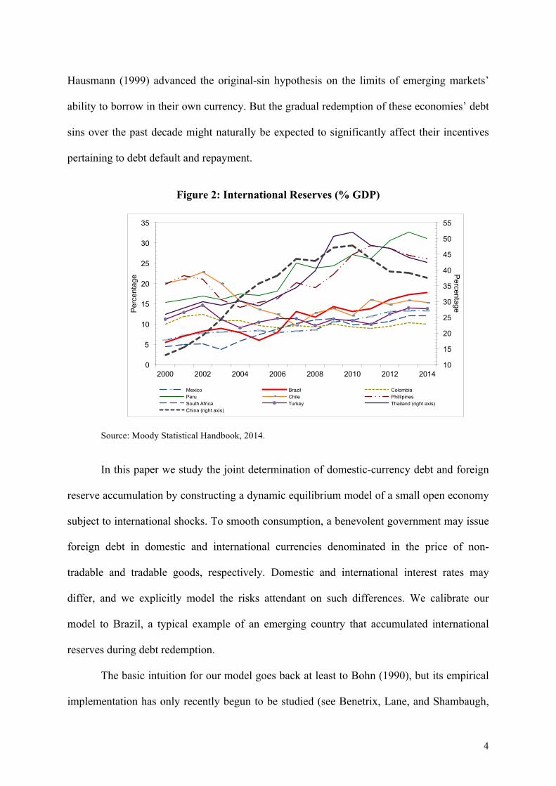
Hausmann (1999) advanced the original-sin hypothesis on the limits of emerging markets’

ability to borrow in their own currency. But the gradual redemption of these economies’ debt

sins over the past decade might naturally be expected to significantly affect their incentives

pertaining to debt default and repayment.

Figure 2: International Reserves (% GDP)

Source: Moody Statistical Handbook, 2014.

In this paper we study the joint determination of domestic-currency debt and foreign

reserve accumulation by constructing a dynamic equilibrium model of a small open economy

subject to international shocks. To smooth consumption, a benevolent government may issue

foreign debt in domestic and international currencies denominated in the price of non-

tradable and tradable goods, respectively. Domestic and international interest rates may

differ, and we explicitly model the risks attendant on such differences. We calibrate our

model to Brazil, a typical example of an emerging country that accumulated international

reserves during debt redemption.

The basic intuition for our model goes back at least to Bohn (1990), but its empirical

implementation has only recently begun to be studied (see Benetrix, Lane, and Shambaugh,

10

15

20

25

30

35

40

45

50

55

0

5

10

15

20

25

30

35

2000 2002 2004 2006 2008 2010 2012 2014

Percentage P

erce

ntag

e

Mexico Brazil Colombia Peru Chile Phillipines South Africa Turkey Thailand (right axis) China (right axis)

5

2015). Having positive net foreign currency positions (assets in foreign, and debt in domestic,

currency) is optimal when a country faces international shocks (as to the endowment of

tradable goods). This is because the asset valuation effects occasioned by currency

depreciation (or appreciation) act to absorb global shocks and smooth consumption.

Debt and reserve accumulation also affect, and are affected by, a country’s incentives

to default. A large stock of domestically denominated debt could help counterbalance an

external shock, but may not be sustainable. A country may not resist the temptation to default

on such debt, through both surprise inflation and outright restructuring of its services. Very

large holdings of international reserves may also not be optimal. International reserves that

are not pledgeable may not increase the sustainability of debt, and in fact, may reduce

sustainability when debt is denominated in foreign currency (Alfaro and Kanczuk, 2009).

Additionally, because holdings of international reserves shift consumption to later dates, they

may be excessively costly.

Our quantitative results suggest that the optimal level of international reserves is

fairly large as their cost is mitigated by valuation-smoothing gains. Our model also matches

some features of Brazil’s economic fluctuations, being consistent, in particular, with the

reduction in exchange rate volatility.

In our analysis, differently from previous work, countries do not accumulate high

levels of reserves to be depleted in “bad” times, as is usually suggested in policy circles.

Instead, issuing domestic debt while accumulating high levels of reserves acts as a hedge

against negative external shocks. This result relates to the vast literature on valuation effects

and optimal international portfolio diversification (Cole and Obstfeld (1991), Engel and

Matsumoto (2009), Alfaro and Kanczuk (2010), Healthcote and Perri (2013), and Gourinchas

and Rey (2014)). We contribute to this literature by explicitly considering a sovereign’s

incentive to default, thus incorporating sustainability of portfolio choices in our analysis. In

6

further contrast to this literature, asset yields and exchange rates are endogenously

determined in the model, and are dependent on the government portfolio choice.

Our paper is also related to the growing literature that examines debt sustainability

(see Aguiar and Amador (2014) and Aguiar et al. (2016) for recent surveys of the literature)

and in particular to the work analyzing the recent increasing role of local-currency debt in

emerging markets (Burger et al. (2012), Du and Schreger (2015 a, b), Hale et al. (2014),

Ottonello and Perez (2017)). More specifically, and differently from this research, our paper

relates to work that examines the determinants of reserve accumulation in emerging markets.

The rationale for reserve accumulation based on interaction with local currency external debt

(i.e., “redemption” of the “original sin”), which was also put forth by Jeanne and Rancière

(2011), complements explanations that emphasize precautionary motives and roll-over risk

(Alfaro and Kanczuk (2009), Durdu, Mendoza, and Terrones (2009) and Bianchi et al.

(2012)), financial stability (Obstfeld, Shambaugh, and Taylor (2010)), externalities associated

with the tradable sector or mercantilist view (Dooley, Folkerts-Landau, and Garber (2003),

and Benigno and Fornaro (2011)) and political economy considerations (Aizenman and

Marion (2003)).

The rest of the paper is organized as follows. In Section 2 we derive intuition from a

two-period, stripped down version of the model. In section 3 we present the infinite-period

general model. In section 4 we calibrate it to the Brazilian economy, and discuss the results

of its quantitative simulation. In Section 5 we present further analysis of the main results and

robustness of the exercises to the volatility of the exchange rate and further discuss exchange-

rate management motivations, debt redemption, and differences between sovereign and

private debt. Section 6 concludes.

7

2 Two-Period Version of Model

We first develop a two-period, stripped down version of the model to provide some

intuition for the joint determination of international reserves and domestically denominated

debt. Although it cannot shed light on the sovereign’s “willingness to pay” incentives, which

hinge on the cost of exclusion from the market, this simpler version underscores how the

combination of reserves and debt both provide insurance against international shocks and

allow for intertemporal consumption smoothing.

In this simple economy, the sovereign consumes only in the second period. In the first

period, she decides her holdings of debt and reserves for the second period, which are

denoted respectively by D and R. The sovereign’s preferences are given by:

u(cN, cT

) = E [log(cN) + log(cT) ],

where households’ second period consumption of non-tradable and tradable goods are

respectively denoted by cN and cT, and E represents expectation. In the first period,

households do not have any endowment, which implies D = R (the first period exchange rate

was normalized to one). In the second period, households receive an endowment of a unit of

consumption of non-tradable good, yN =1, and their endowment of the tradable good follows

a stochastic process:

yTG = (1 + σ) , with probability equal to ½ (good state of nature), and

yTB = (1 – σ) , with probability equal to ½ (bad state of nature).

Reserves correspond to riskless bonds that bear interest rates given by ρ. Debt can be

issued both in foreign currency and in domestic currency. We assume the sovereign to repay

debt in both the good and bad states of nature. That is, default cannot be used to smooth

consumption.

8

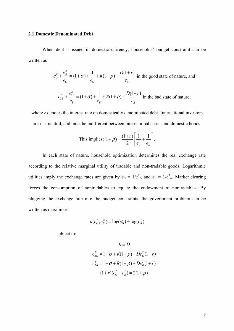
2.1 Domestic Denominated Debt

When debt is issued in domestic currency, households’ budget constraint can be

written as

GGG

NGT

G erDR

eecc )1()1(1)1( +−++++=+ ρσ in the good state of nature, and

BBB

NBT

B erDR

eecc )1()1(1)1(2

2+−++++=+ ρσ in the bad state of nature,

where r denotes the interest rate on domestically denominated debt. International investors

are risk neutral, and must be indifferent between international assets and domestic bonds.

This implies: ⎥⎦

⎤⎢⎣

⎡++=+

BG eer 112)1()1( ρ .

In each state of nature, household optimization determines the real exchange rate

according to the relative marginal utility of tradable and non-tradable goods. Logarithmic

utilities imply the exchange rates are given by eG = 1/cTG and eB = 1/cT

B. Market clearing

forces the consumption of nontradables to equate the endowment of nontradables. By

plugging the exchange rate into the budget constraints, the government problem can be

written as maximize:

)log()log(),( TB

TG

NB

TG ccccu +=

subject to:

)1(2))(1(

)1()1(1

)1()1(1

2

2

ρ

ρσ

ρσ

+=++

+−++−=

+−+++=

=

TB

TG

TB

TB

TG

TG

ccr

rDcRc

rDcRc

DR

9

To derive some intuition, before considering that D = R, suppose that cT2G + cT

2B

equals approximately two, such that the last constraint can be approximately written as r = ρ.

In this case, it becomes straightforward to plug the constraints into the maximization as

follows,

⎟⎟⎠

⎞⎜⎜⎝

⎛++++−+⎟⎟⎠

⎞⎜⎜⎝

⎛+++++=

)1(1)1(1log

)1(1)1(1log

ρρσ

ρρσ

DR

DRu ,

To make consumption the same in the good and bad states, the government could set either a

very high D or very high R, or both. Since D = R, the solution is to make them both very

high. (Note that, as a consequence, it is indeed the case that cT2G + cT

2B equals two, and that r

= ρ).

2.2 Foreign Denominated Debt

If debt is issued in foreign currency, the household’s budget constraint would be

written as:

)1()1(1)1( rDRee

ccGG

NGT

G +−++++=+ ρσ in the good state of nature, and

)1()1(1)1( rDRee

ccBB

NBT

B +−++++=+ ρσ in the bad state of nature.

and, since there is no default, ρ = r.

As before, to derive some intuition and before considering that D = R, we plug the

exchange rates obtained by the market clearing condition to obtain the government problem

))1)((1log())1)((1log( ρσρσ +−+−++−++= DRDRu ,

To make consumption the same in both states, the government would have to make (R

– D) very large. Of course this is not possible, as D = R. This happens because the

10

government has no instrument to redistribute resources across states of nature, only across

different time periods.

The conclusion of this section is that domestic denominated debt provides the

government a natural way to insure against income shocks. Additionally, this simplified two-

period model underscores how reserves can be used to cancel out the intertemporal transfers

of resources that are caused by the issuance of domestic denominated bonds. In contrast,

foreign denominated debt cannot provide the same intratemporal insurance, as it only

transfers resources across time.

Because the two–period model abstracts from default incentives, it cannot shed light

on the amount of debt and reserves a sovereign chooses to accumulate. The next section

tackles these issues.

3 General Model

We model an economy populated by a continuum of private households, a benevolent

government, and a continuum of international, risk-neutral investors. Preferences are

concave, implying that households prefer a smooth consumption profile for both tradable and

non-tradable goods. To smooth consumption, a benevolent government may optimally issue

foreign debt in domestically denominated currency and accumulate foreign reserves. The

benevolent government may further optimally choose to default on its international

commitments, in which case we assume it to be temporarily excluded from borrowing in

international markets. Default can be thought as surprise inflation or as an outright default.1

1 Reinhart and Rogoff (2009) document the main stylized facts regarding sovereign debt and default. As the authors document, the cases of full outright default, as are those of outright repudiation of domestic debt, are rare. Historical average haircut of outright default was around 30%. In other words, the assumption of full default is a useful simplification both in the case of inflation and outright default.

11

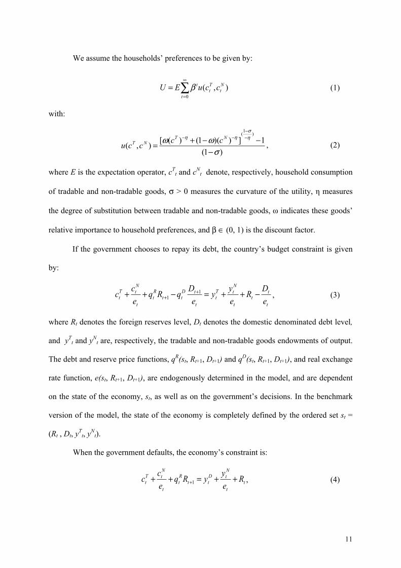
We assume the households’ preferences to be given by:

∑∞

=

=0

),(t

Nt

Tt

t ccuEU β (1)

with:

)1(

1]))(1()([),()1(

σωω η

σηη

−−−+=

−−

−− NTNT ccccu , (2)

where E is the expectation operator, cTt and cN

t denote, respectively, household consumption

of tradable and non-tradable goods, σ > 0 measures the curvature of the utility, η measures

the degree of substitution between tradable and non-tradable goods, ω indicates these goods’

relative importance to household preferences, and β ∈ (0, 1) is the discount factor.

If the government chooses to repay its debt, the country’s budget constraint is given

by:

t

tt

t

NtT

tt

tDtt

Rt

t

NtT

t eDR

eyy

eDqRq

ecc −++=−++ +

+1

1 , (3)

where Rt denotes the foreign reserves level, Dt denotes the domestic denominated debt level,

and yTt and yN

t are, respectively, the tradable and non-tradable goods endowments of output.

The debt and reserve price functions, qR(st, Rt+1, Dt+1) and qD(st, Rt+1, Dt+1), and real exchange

rate function, e(st, Rt+1, Dt+1), are endogenously determined in the model, and are dependent

on the state of the economy, st, as well as on the government’s decisions. In the benchmark

version of the model, the state of the economy is completely defined by the ordered set st =

(Rt , Dt, yTt, yN

t).

When the government defaults, the economy’s constraint is:

tt

NtD

ttRt

t

NtT

t ReyyRq

ecc ++=++ +1 , (4)

12

where yD corresponds to the endowments of tradable goods in default periods. After

defaulting, the sovereign is temporarily excluded from issuing debt. We assume θ to be the

probability that the sovereign regains full access to international credit markets.

International investors are risk-neutral and have an opportunity cost of funds given by

ρ, which denotes the risk-free rate denominated in the price of tradable goods. Investors will

choose the debt and reserve prices, qD and qR, which depend on the perceived likelihood of

default and currency depreciation. For these investors to be indifferent between the riskless

asset and lending in a country’s non-tradable goods denomination, it must be the case that,

⎥⎦

⎤⎢⎣

⎡−

+=

++

11)1(

)1(1

t

ttt

Dt e

edEq

ρ (5)

and ρ+

=11Rq (6)

where dt+1 ϵ {0, 1}t is the occurrence (or not) of default, which is endogenously determined

and depends on the sovereign’s incentives to repay the debt. Note (5) is a version of the

uncovered interest parity condition that considers the possibility of default.

Because the government chooses debt and reserve levels, the problem of the

households is intratemporal, and has the sole role of determining the real exchange rate.

Individual household maximization equates the relative marginal utility of tradables to non-

tradables to their relative prices,

η

ωω

+

⎟⎟⎠

⎞⎜⎜⎝

⎛−

=1

)1( Tt

Nt

t cce . (7)

The market-clearing condition for non-tradable goods is:

Nt

Nt yc = . (8)

The timing of the decisions is as follows. In the beginning of each period, the

government starts with debt level Dt and reserve level Rt and receives endowments yTt and

13

yNt. It faces the reserve price schedule qR(st, Rt+1, Dt+1), bond price schedule qD(st, Rt+1, Dt+1),

and real exchange rate price schedule e(st, Rt+1, Dt+1). Taking these schedules as given, the

government simultaneously makes three decisions. It chooses (i) the next level of reserves,

Rt+1, (ii) whether to default on the debt, and (iii) if it decides not to default, the next level of

debt, Dt+1.

The model described is a stochastic dynamic game. We focus exclusively on the

Markov perfect equilibria, whereby the government does not have commitment and players

act sequentially and rationally.

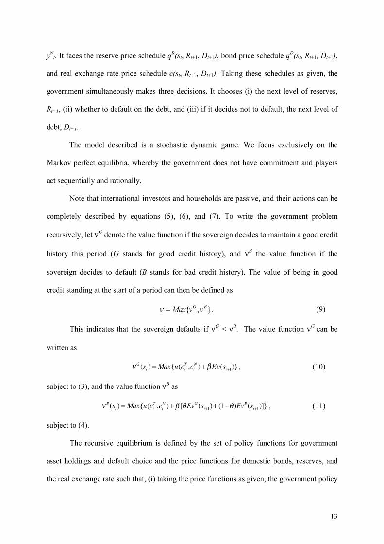
Note that international investors and households are passive, and their actions can be

completely described by equations (5), (6), and (7). To write the government problem

recursively, let νG denote the value function if the sovereign decides to maintain a good credit

history this period (G stands for good credit history), and νB the value function if the

sovereign decides to default (B stands for bad credit history). The value of being in good

credit standing at the start of a period can then be defined as

},{ BG vvMax=ν . (9)

This indicates that the sovereign defaults if νG < νB. The value function νG can be

written as

νG (st ) = Max{u(ctT ,ct

N )+ βEv(st+1)} , (10)

subject to (3), and the value function νB as

ν B (st ) = Max{u(ctT ,ct

N )+ β [θEvG (st+1)+ (1−θ )EvB (st+1)]} , (11)

subject to (4).

The recursive equilibrium is defined by the set of policy functions for government

asset holdings and default choice and the price functions for domestic bonds, reserves, and

the real exchange rate such that, (i) taking the price functions as given, the government policy

14

functions satisfy the government optimization problem, and (ii) prices of domestic bonds,

reserves, and the exchange rate are consistent with the government decisions.

This definition of equilibrium, identical to that of Arellano (2008) and Alfaro and

Kanczuk (2005, 2009), among many others, reflects a game played by a large agent (the

government) against many small agents (the continua of investors and households). It implies

that the government internalizes the effects of its actions over the prices. In our model, the

government internalizes the effect of its asset holdings over the real exchange rate.

4 Quantitative Analysis

We solve the model numerically to evaluate its quantitative predictions regarding the

accumulation of debt and reserves, the occurrence of default events and the business cycle

properties of the exchange rate.

4.1 Calibration

A difficulty in performing the quantitative analysis is that emerging countries only

began to issue relevant amounts of domestically-denominated bonds in the middle of the past

decade. The data time span of the current regime, especially as concerned with episodes of

default, is consequently relatively small. In Brazil, for example, the last default episode was

between 1983 and 1990 (Reinhart, 2010).

We address this problem by calibrating some of the parameters using a much longer

time horizon, during which international debt was denominated mainly in foreign currency.

In transforming our economy to consider the case in which bonds were denominated in

foreign currency, we assume the country budget constraint to be given by

ttt

NtT

ttBtt

Rt

t

NtT

t BReyyBqRq

ecc −++=−++ ++ 11 (3’)

15

rather than equation (3).

This is effectively the case considered by Alfaro and Kanczuk (2009), in which B

denotes holdings of foreign bonds denominated in foreign currency. As above, in the case of

a debt default, reserves R continue to be held and can be used to smooth consumption. We

proceed with calibration by considering annual data since 1965.

We set the international interest rate ρ = 0.04 and inter-temporal substitution

parameter σ = 2, as is usual in real-business-cycle research in which each period corresponds

to one year (see Kanczuk, 2004). There being considerable disagreement about the

intratemporal elasticity of substitution between tradable and non-tradable goods (Akinci,

2011), we make elasticity equal to one (the middle of the many possible estimations), and, for

that, set η = 0. Our results are robust to many other parameter values. For the weight of

tradables, we use the share of output that corresponds to industry and agriculture, and set ω =

0.35, which is also consistent with literature estimations.

Because non-tradable consumption goods cannot be smoothed, we focus on the case

in which shocks are exclusively external, that is, on the tradable endowment.2 We thus make

yN = 1 for all periods. We then set yTt = exp (zT

t), and assume that zTt can take a finite number

of values and that it evolves over time according to a Markov transition matrix with elements

πT(zTi , zT

j ); that is, the probability that zTt +1 = zT

j, given that zTt = zT

i, is given by the matrix π

element of row i and column j.

We calibrate the technology state zT by considering the (logarithm) of the GDP to

follow an AR(1) process; that is, zt+1T =α zt

T + ε t+1 where ε t ≈ N (0,σε2 ) . We obtain α = 0.85

and σ = 0.12. The apparently high value of the standard deviation reflects the fact that the

2 Since the consumption of non-tradeable goods must be always equal to the non-tradeable endowment, domestic shocks cannot be smoothed out. Different debt and reserve levels could still affect allocations due to the valuation effects, albeit quantitatively small, that result from the exchange rate movements.

16

tradable sector corresponds to roughly one-third of total output. To make the model

consistent with the data, the volatility of the tradable sector must thus be about three times

that of total output. As an indirect indication of consistency, we note that the volatility of the

industry and agriculture output is three times as high as the Brazilian GDP.

We discretize this technology state into nine possible values, spaced such that the

extreme values are three standard deviations away from the mean. We also discretize the

space state of debt and reserves enough (400 grid points) to avoid spurious results.

Setting the probability of redemption at θ = 0.5 implies an average stay in autarky of

two years, in line with estimates by Gelos et al. (2011). Direct output costs are modeled from

default and assumed to be asymmetric: yD = yDEF in case yD > yDEF. Setting yDEF = 0.85yT

implies that tradable output costs of defaulting equal 15%, the relatively large number again

reflecting the fact that the tradable sector corresponds to one-third of the economy.

To obtain reasonable levels of debt in equilibrium, we set the intertemporal factor at

the relatively low value of β = 0.80, which is common practice in debt models (Alfaro and

Kanczuk, 2009). This calibration also sets the debt service (as a fraction of GDP) and the

interest spread equal to their observed levels, which are 3.3% and 6.8%, respectively.

Table 1 summarizes the parameter values.

Table 1: Calibration

Technology autocorrelation α = 0.85

Technology standard deviation σ ε = 0.12

Probability of redemption θ = 0.50

Output costs yDEF = 0.85yT

Risk aversion σ = 2

Risk free interest rate ρ = 0.04

Discount factor β = 0.80

17

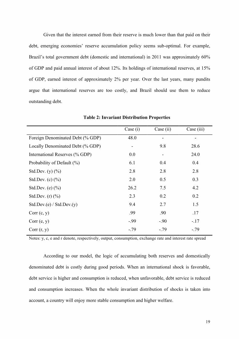
4.2 Simulation results

We first simulate our economy under the assumption that debt is denominated in

foreign currency. For the chosen parameters, the invariant distribution displays 48% of GDP

of debt and a 6.1% frequency of default (case (i) in Table 2). These numbers are very much

in line with the historical data for Brazil and other emerging countries presented in many

other papers. The equilibrium level of reserves is zero, a reincarnation of Alfaro and

Kanczuk’s (2009) result in a model with two sectors (but shocks in only one).

As discussed extensively in that paper, there is a potential role in this setup for

reserves to be used to smooth consumption when the country is excluded from international

markets. But, because reserve holdings reduce the sustainability of debt, quantitatively their

optimal holding is zero. The optimal government policy is to hold (foreign denominated) debt

and default in extremely bad times.

As an intermediate step, assuming the government cannot hold reserves (case (ii)), we

simulate the economy with locally denominated bonds. We obtain, in this case, that the

government holds a fairly small amount of debt (9.8% of GDP) and virtually does not default.

Note that the volatility (standard deviation) of the exchange rate drops from 26.2% in the

case of foreign-denominated debt to 7.5% in the case of domestically-denominated debt with

no reserves. Thus, even without resorting to default, domestic denomination results in more

consumption smoothing.

The level of domestic denominated debt is small because consumption smoothing can

be attained even without default. Defaulting has the benefit of smoothing consumption but it

has its costs: the exclusion of markets and output drop itself. Since the benefit of smoothing

is not needed, the sovereign opts to choose a level of debt in which she can resist defaulting.

18

When we simulate the economy with locally denominated bonds, but allow the

government to hold positive amounts of reserves (case (iii)), we obtain that, in the invariant

distribution, the economy displays 28.6% of GDP in (locally denominated) debt, with 24% of

GDP in reserves. As in case (ii), the government virtually does not resort to default as a

means to smooth consumption. Note also that the volatility of consumption drops even more,

the standard deviation of the exchange rate falling to 4.2.

The intuition for holding both (domestically denominated) debt and reserves,

developed in Section 2, is to allow for consumption smoothing across both states and time.

But the experiment with the full-fledged model yields some novel results.

In the two-period model, optimal policy was to accumulate infinite amounts of debt

and reserves. In the general model, default incentives and the related issue of debt

sustainability, reduce the amount of optimal debt and reserves. That they may, in fact, be

smaller than anticipated suggests that this scheme for smoothing consumption is fairly

powerful.

A second insight is that accumulation of reserves is not a problem in terms of

reducing the sustainability of debt when debt is in local currency. The experiment shows the

proposed scheme to be, in fact, sustainable in the sense that the government (almost) never

defaults.

Put differently, in both the foreign denominated and locally denominated debt

experiments, international reserves play a role when a country is excluded from capital

markets. However, this role reduces the amount of debt that is sustainable, triggering

defaults, which are costly. When debt is foreign denominated, Alfaro and Kanczuk (2009)

obtain that the optimal level of reserves is zero. This paper indicates that, when debt is

domestically denominated, reserves are very useful, owing to their valuation effect, which

helps smooth consumption.

19

Given that the interest earned from their reserve is much lower than that paid on their

debt, emerging economies’ reserve accumulation policy seems sub-optimal. For example,

Brazil’s total government debt (domestic and international) in 2011 was approximately 60%

of GDP and paid annual interest of about 12%. Its holdings of international reserves, at 15%

of GDP, earned interest of approximately 2% per year. Over the last years, many pundits

argue that international reserves are too costly, and Brazil should use them to reduce

outstanding debt.

Table 2: Invariant Distribution Properties

Case (i) Case (ii) Case (iii)

Foreign Denominated Debt (% GDP) 48.0 -   -  

Locally Denominated Debt (% GDP) - 9.8   28.6  

International Reserves (% GDP) 0.0 -   24.0  

Probability of Default (%) 6.1 0.4   0.4  

Std.Dev. (y) (%) 2.8 2.8   2.8  

Std.Dev. (c) (%) 2.0 0.5   0.3  

Std.Dev. (e) (%) 26.2 7.5   4.2  

Std.Dev. (r) (%) 2.3 0.2   0.2  

Std.Dev.(e) / Std.Dev.(y) 9.4 2.7   1.5  

Corr (c, y) .99 .90   .17  

Corr (e, y) -.99 -.90   -.17  

Corr (r, y) -.79 -.79   -.79  

Notes: y, c, e and r denote, respectively, output, consumption, exchange rate and interest rate spread

According to our model, the logic of accumulating both reserves and domestically

denominated debt is costly during good periods. When an international shock is favorable,

debt service is higher and consumption is reduced, when unfavorable, debt service is reduced

and consumption increases. When the whole invariant distribution of shocks is taken into

account, a country will enjoy more stable consumption and higher welfare.

20

Note that in the proposed construction, the level of reserves remains high during

unfavorable periods. Contrary to the usual argument in policy circles, reserves are thus not

insurance that can be “used” in bad times. The idea is not to buy consumption goods that

deplete the stock of reserves, but rather to maintain a constant reserve stock that serves as

insurance by increasing the stabilizing effect of domestic-denominated debt.

In fact, the optimal policy function is to hold the amount of debt and reserves next

period constant in the relevant region, regardless of the period state. For this reason, we opted

not to depict the debt and reserve policy functions, since they are just simple horizontal lines.

The essential intuition is that the stabilization effect of issuing local-currency debt results in

sufficient consumption smoothing that there is no need to change the levels of debt and

reserves.

4.3 Comparison with the Brazilian data

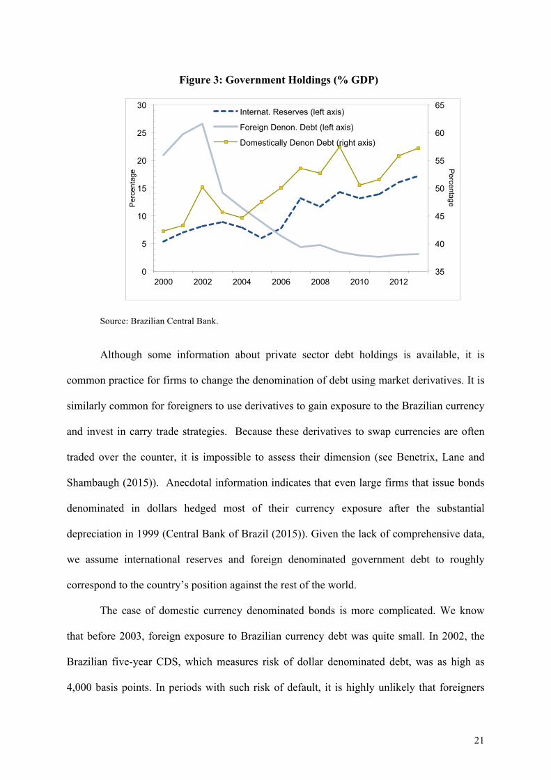
We now compare the model’s outcomes with recent data from Brazil. Figure 3 plots

the evolution of government holdings of international reserves and foreign and domestically

denominated debt. These assets (or liabilities) could potentially be held against both the

Brazilian private sector and the rest of the world.

In our model, only the government is assumed to be able to hold international assets.

However, the position of the full country (government and private sector) against the rest of

the world is, in fact, the closest real concept to be contrasted with the model, the challenge in

doing so being the absence of comprehensive data about the denomination of private sector

holdings.

21

Figure 3: Government Holdings (% GDP)

Source: Brazilian Central Bank.

Although some information about private sector debt holdings is available, it is

common practice for firms to change the denomination of debt using market derivatives. It is

similarly common for foreigners to use derivatives to gain exposure to the Brazilian currency

and invest in carry trade strategies. Because these derivatives to swap currencies are often

traded over the counter, it is impossible to assess their dimension (see Benetrix, Lane and

Shambaugh (2015)). Anecdotal information indicates that even large firms that issue bonds

denominated in dollars hedged most of their currency exposure after the substantial

depreciation in 1999 (Central Bank of Brazil (2015)). Given the lack of comprehensive data,

we assume international reserves and foreign denominated government debt to roughly

correspond to the country’s position against the rest of the world.

The case of domestic currency denominated bonds is more complicated. We know

that before 2003, foreign exposure to Brazilian currency debt was quite small. In 2002, the

Brazilian five-year CDS, which measures risk of dollar denominated debt, was as high as

4,000 basis points. In periods with such risk of default, it is highly unlikely that foreigners

35

40

45

50

55

60

65

0

5

10

15

20

25

30

2000 2002 2004 2006 2008 2010 2012

Percentage P

erce

ntag

e

Internat. Reserves (left axis)

Foreign Denon. Debt (left axis)

Domestically Denon Debt (right axis)

22

would hold local currency. Post-2002, because the increase in debt was concomitant with the

accumulation of reserves, as depicted in Figure 3, it is natural to assume foreigners to be

responsible for a large fraction of it.

Table 3 summarizes the data. Rather than guessing the holdings of assets and

liabilities, we indicate the net position in each denomination. Before 2006, there was virtually

no local-denominated external debt. After 2006, holdings of reserves were higher than

holdings of foreign denominated debt. Thus, the net position of foreign denominated

securities switched from debt (liabilities) to assets (reserves).

Table 3: Brazilian Data

1996 to 2005 2006 to 2014

Foreign Denominated Debt Assets (Reserves)

Locally Denominated 0 Debt

Std. Dev. (y) (%) 3.0 2.2

Std. Dev. (c) (%) 6.0 3.3

Std. Dev. (e) (%) 35.9 12.3

Sdt. Dev.( r) (%) 3.8 1.4

Std. Dev. (e)/Std. Dev. (y) 11.8 5.6

Corr (c, y) 0.92 0.69

Corr (e, y) -0.90 -0.87

Corr (r, y) -0.69 0.14

Mean (r) (%) 7.7 1.4

Notes: y, c, e and r denote, respectively, output, consumption, exchange rate and interest spread

Information about the cyclical behavior of output and the real exchange rate is

presented in Figure 4. There being no available data on the consumption of tradables and

non-tradables, we choose the exchange rate as the primary variable to contrast with the

model. The sample being short, a single crisis could imply differing output volatility. We

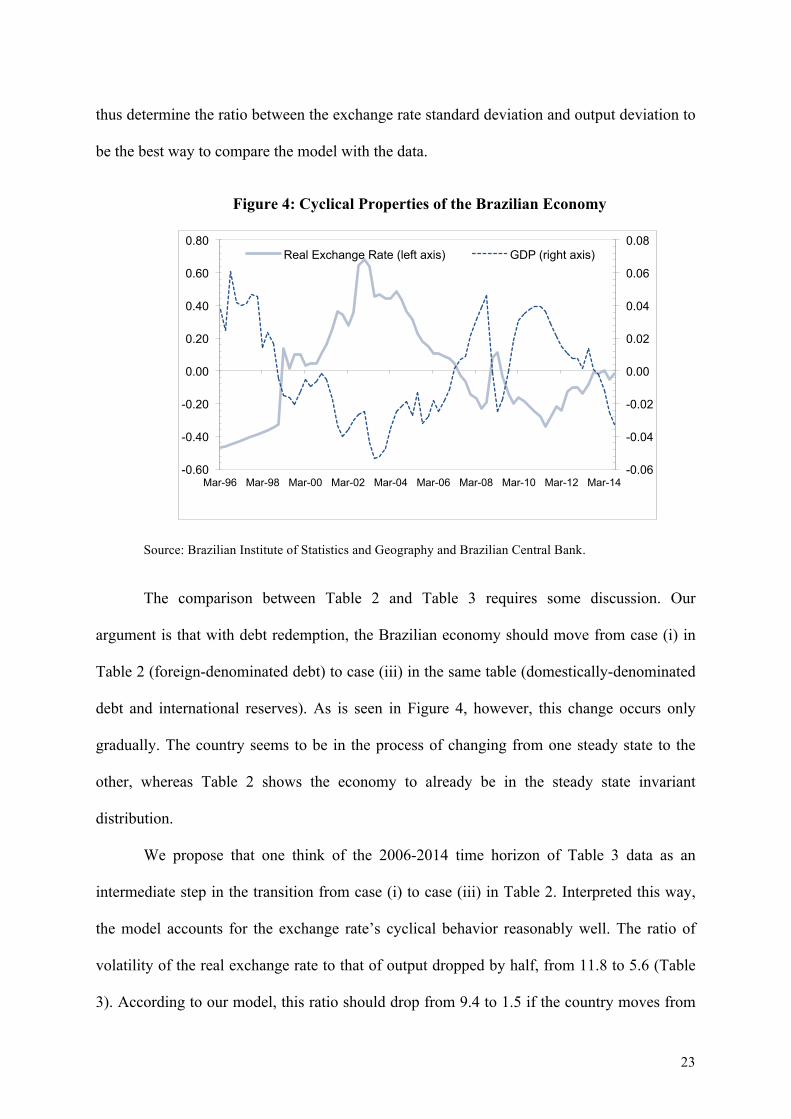
23

thus determine the ratio between the exchange rate standard deviation and output deviation to

be the best way to compare the model with the data.

Figure 4: Cyclical Properties of the Brazilian Economy

Source: Brazilian Institute of Statistics and Geography and Brazilian Central Bank.

The comparison between Table 2 and Table 3 requires some discussion. Our

argument is that with debt redemption, the Brazilian economy should move from case (i) in

Table 2 (foreign-denominated debt) to case (iii) in the same table (domestically-denominated

debt and international reserves). As is seen in Figure 4, however, this change occurs only

gradually. The country seems to be in the process of changing from one steady state to the

other, whereas Table 2 shows the economy to already be in the steady state invariant

distribution.

We propose that one think of the 2006-2014 time horizon of Table 3 data as an

intermediate step in the transition from case (i) to case (iii) in Table 2. Interpreted this way,

the model accounts for the exchange rate’s cyclical behavior reasonably well. The ratio of

volatility of the real exchange rate to that of output dropped by half, from 11.8 to 5.6 (Table

3). According to our model, this ratio should drop from 9.4 to 1.5 if the country moves from

-0.06

-0.04

-0.02

0.00

0.02

0.04

0.06

0.08

-0.60

-0.40

-0.20

0.00

0.20

0.40

0.60

0.80

Mar-96 Mar-98 Mar-00 Mar-02 Mar-04 Mar-06 Mar-08 Mar-10 Mar-12 Mar-14

Real Exchange Rate (left axis) GDP (right axis)

24

one steady state to the other (Table 2). Brazil, however, is still far from converging on the

steady state. During the 2006-2014 period, Brazil’s holdings of international reserves were

13.4% of GDP. In the proposed steady state, these holdings will reach 24% of GDP.

For completeness, Table 3 also reports consumption standard deviations, as a

secondary indication of the volatility reduction. We observe that the volatility of consumption

also drops in Brazil, both in absolute value and as a fraction of GDP volatility. However, the

mere fact that the volatility of consumption is a lot higher than GDP volatility questions the

use of consumption in the place of exchange rate. Measurement problems with Brazilian data

and other issues (common to other emerging countries) render consumption volatility a

particularly noisy information.

Table 3 additionally depicts the correlation of the exchange rate and output. For the

two periods considered, the correlation was -0.90 and -0.87. In our model, there being shocks

only to tradable-goods, this correlation is equals to -0.99 in case (i). A simple way to reduce

this correlation would be to add (uncorrelated) shocks to the non-tradable sector. We

nevertheless construe this comparison to support our hypothesis that non-tradable sector

shocks are not a quantitatively important factor in our analysis. Consumption smoothing by

itself makes this correlation very low, once domestic debt is considered.

Finally, Table 3 reports the correlation between the spread and output. In the first

period the correlation is negative, as expected. In the second period it turns positive, but very

small. This happened because, with the recent reduction of risk, spreads converged to fairly

small values, and became largely irrelevant for the understanding of other variables.

25

4.4 Evidence from other Emerging Countries

We now look at some data evidence for other emerging countries. As we mentioned

in the introduction, accumulation of domestic denominated debt in conjunction with reserves

is becoming a ubiquitous phenomenon. This generates several questions: Are the countries

that accumulate more debt the ones that are more subjected to international shocks? Has the

volatility of the exchange rate dropped more in countries that accumulated more debt?

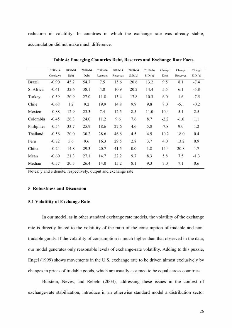
Although a formal analysis is beyond the scope of this paper, in Table 4 we report

some statistics for countries depicted in Figures 1 and 2, for which Moody offers complete

data. As a word of caution, since the time span covered is very short, it becomes statistically

difficult to capture changes. We opted to define two periods, the first containing the years

from 2000 to 2004, the second defined by the period 2010 to 2014, to calculate the averages

of the variables. We then obtain the change in the stock of debt, the stock of reserves and the

standard deviation of the exchange rate between these two periods.

Even though the data sample is very small, it provides some statistics consistent with

intuition. In particular, the correlation between (domestically denominated) debt

accumulation and exchange rate volatility reduction is positive. It is also the case that debt

accumulation is positively correlated with reserve accumulation. On the other hand, we note

that for many countries there was an increase in exchange rate volatility, in spite of debt and

reserves accumulation.

We believe the best way to look at table 4 is to divide the countries into those where

the exchange rate was very volatile (Brazil, South Africa and Turkey), and those in which the

exchange rate was already fairly stable in the first period considered (Philippines, Thailand,

Peru, China). In the countries in which the exchange rate was very volatile, the accumulation

of (domestically denominated) debt and reserves had an important effect, and caused a

26

reduction in volatility. In countries in which the exchange rate was already stable,

accumulation did not make much difference.

Table 4: Emerging Countries Debt, Reserves and Exchange Rate Facts

2000-14

Corr(e,y)

2000-04

Debt

2010-14

Debt

2000-04

Reserves

2010-14

Reserves

2000-04

S.D.(e)

2010-14

S.D.(e)

Change

Debt

Change

Reserves

Change

S.D.(e)

Brazil   -0.90 45.2 54.7 7.5 15.6 20.6 13.2 9.5 8.1 -7.4

S. Africa   -0.41 32.6 38.1 4.8 10.9 20.2 14.4 5.5 6.1 -5.8

Turkey   -0.59 20.9 27.0 11.8 13.4 17.8 10.3 6.0 1.6 -7.5

Chile   -0.68 1.2 9.2 19.9 14.8 9.9 9.8 8.0 -5.1 -0.2

Mexico   -0.88 12.9 23.3 7.4 12.5 8.5 11.0 10.4 5.1 2.5

Colombia   -0.45 26.3 24.0 11.2 9.6 7.6 8.7 -2.2 -1.6 1.1

Philipines   -0.54 33.7 25.9 18.6 27.6 4.6 5.8 -7.8 9.0 1.2

Thailand   -0.56 20.0 30.2 28.6 46.6 4.5 4.9 10.2 18.0 0.4

Peru   -0.72 5.6 9.6 16.3 29.5 2.8 3.7 4.0 13.2 0.9

China   -0.24 14.8 29.3 20.7 41.5 0.0 1.8 14.4 20.8 1.7

Mean   -0.60 21.3 27.1 14.7 22.2 9.7 8.3 5.8 7.5 -1.3

Median   -0.57 20.5 26.4 14.0 15.2 8.1 9.3 7.0 7.1 0.6

Notes: y and e denote, respectively, output and exchange rate

5 Robustness and Discussion

5.1 Volatility of Exchange Rate

In our model, as in other standard exchange rate models, the volatility of the exchange

rate is directly linked to the volatility of the ratio of the consumption of tradable and non-

tradable goods. If the volatility of consumption is much higher than that observed in the data,

our model generates only reasonable levels of exchange-rate volatility. Adding to this puzzle,

Engel (1999) shows movements in the U.S. exchange rate to be driven almost exclusively by

changes in prices of tradable goods, which are usually assumed to be equal across countries.

Burstein, Neves, and Rebelo (2003), addressing these issues in the context of

exchange-rate stabilization, introduce in an otherwise standard model a distribution sector

27

that can dramatically improve the model’s performance. Rather than adding a new sector to

our model, we invoke their claim that modifying preferences in a standard model can mimic

the introduction of distribution costs.

We modify, in particular, the utility function, making the share of tradable goods ω =

0.10. As above, we find the optimal policy to be the accumulation of reserves in conjunction

with locally denominated debt, and this strategy to be effective at smoothing consumption

across both different states of nature and time. The only difference between the results of this

experiment and the one in Section 4 is quantitative. In this alternative economy, the levels of

local-currency debt and reserves as a percentage of GDP are, respectively, 10.4% and 3.2%.

Thus, the decrease in the importance of the tradable sector implies, as expected, a reduction

in debt and reserve accumulation.

5.2 Reserve Accumulation and Exchange Rate Management

A branch of the literature on reserve accumulation argues that government motivation

is a form of exchange rate management (Dooley et al., 2003). That is, reserve accumulation is

a means of keeping the exchange rate depreciated and thereby helping to protect a country’s

industry and stimulate exports. In this paper we do not consider mercantile considerations for

reservation accumulation. For example, as the commodity boom ended, and growth slowed

down, some countries have used some of their international reserves to maintain their peg.

Our paper abstracts from this motivation. However, this has clearly not been the main driver

for all countries. Brazil, for example, maintained roughly the same reserve management

policy independently of commodity prices.

Notice that while in the present paper reserves are used to smooth the volatility of the

exchange rate, in the literature on reserves and export-led growth reserves are used to

influence the average value of the exchange rate. That is, in our model, the rationale for

28

reserve accumulation is to smooth consumption of tradable goods. But as a direct

consequence the exchange rate is also smoothed. In particular, the exchange rate does not

appreciate as much in good times due to the accumulation of reserves. As the commodity

boom ended, and growth slowed down, some countries have used some of their international

reserves in order to maintain their peg. Our paper abstracts from this motivation. However,

this has clearly not been the main driver for all countries.

5.3 Rationale for Debt Redemption

In our model, debt redemption, or the possibility of a country issuing external debt

denominated in local currency, because it implies fewer occurrences of default, does not

explain why emerging countries were unable to issue domestically-denominated external debt

previously, such as during the 1980s and into the 1990s. Although a complete investigation is

beyond the scope of this paper, we conjecture that there were two reasons for debt

redemption.

One possibility is that investors could not identify the type of government issuing the

bonds. As Alfaro and Kanczuk (2005) argue, sovereign-default episodes (delays,

rescheduling, etc.) seem consistent with reputation building. This, in turn, is consistent with

the existence of different types of governments including those that would default

independently of the state of nature (“inexcusable defaults” in the language of Grossman and

Van Huyck (1988)). Lenders, when extracting the information from the default in order to

set the next period’s interest rate, most likely will consider the possibility that in this period

the sovereign was of the “bad” type and charge higher interest rates. It is possible that risk

increased sufficiently to shut down the market. As the type of government in control became

clearer, and the risk was reduced, international investors became more disposed to buy debt

issued in local markets.

29

A second, related issue is inflation. Inflation and inflation volatility were extremely

high in Latin America during the 1980s, making returns on domestic-denominated bonds

very risky for international investors, possibly so high that investor appetite for this type of

asset was insufficient for the existence of the market.

5.4 Private-Sector Debt

In our model, debt is issued exclusively by the benevolent government; households

(i.e., the private sector) cannot issue debt and choose their inter-temporal consumption. This

assumption raises two issues. First, the analysis would be unchanged were private sector debt

to be included, assuming no distortions or other imperfections (taxes, externalities, time

inconsistency issues) that could drive a wedge between the objectives of the benevolent

government and those of the households. Second, in the event that the objectives of the

government and the households do conflict, the government could attempt to offset, perhaps

even prohibit, household debt and reserve accumulation by creating rules and changing the

law. Thus, unless political economy issues are considered, the assumption that households

cannot issue debt is not crucial to the analysis.

As mentioned before, since firms often use over-the-counter derivatives to change

their debt denomination, data on private debt is not really reliable to assess net positions.

These considerations notwithstanding, due to the recent Real depreciation, and the

consequent balance sheets risk, the Central Bank of Brazil conducted an inquiry on corporate

businesses to have a sense of the dimension of potential currency risks. As Table 5 indicates,

dollar denominated corporate risk debt seemed fairly small. In particular, unhedged debt of

firms that have no foreign counterpart amounted to only 3.3% of GDP. This suggests that our

assumption that only the government holds international debt seems adequate from a purely

quantitative viewpoint as well.

30

Table 5: Dollar Denominated Corporate Debt in June 2015

Type of Firm Debt (% GDP) Non exporter, with local hedge   4.0  

Non exporter, multinational   2.1  Non exporter, with international assets   3.6  

Non exporter, without hedge   3.3  

Source: Central Bank of Brazil

6 Conclusion

The past decade was characterized by two new trends in international capital flows to

emerging markets, (1) carry trade activity and associated foreign participation in local-

currency bond markets, and (2) large accumulations of international reserves. We believe that

both can be rationalized as optimal debt management strategy. Borrowing in domestic

currency can insure emerging countries against international shocks because the valuation

effect that results from currency appreciation has a negative correlation with the shock, an

intuition that dates to Bohn (1990).

We revisit sovereign debt sustainability under the assumptions that countries can

accumulate reserves and borrow internationally using their own currency. Countries do not

accumulate reserves to be depleted in “bad” times. Instead, issuing domestic debt while

accumulating reserves acts as a hedge against external shocks. Asset-valuation effects due to

currency fluctuations act to absorb global shocks and render consumption smoother. Our

quantitative study of how reserve accumulation affects governments’ decisions to default

finds that optimal holdings turn out to be as large as those presently observed. Our results

match some of the characteristics of the Brazilian business cycle suggesting this strategy to

be effective for smoothing consumption and reducing the occurrence of default.

31

References

Aguiar, Mark, and Manuel Amador (2014). “Sovereign Debt.” In Handbook of International

Economics, vol. 4, eds. G. Gopinath, E. Helpman and K. Rogoff, Elsevier.

Aguiar, Mark, Satyajit Chatterjee, Harald Cole, and Zachary Stangebye. 2016. “Quantitative

Models of Sovereign Debt Crises,” Handbook of Macroeconomics, vol. 4, eds. Harald

Uhlig and John Taylor.

Aizenman, Joshua, and Nancy Marion (2003). “International Reserve Holdings with

Sovereign Risk and Costly Tax Collection,” The Economic Journal 114, 569-591.

Akinci, Orze (2011). “A Note on the Estimation of the Atemporal Elasticity of Substitution

between Tradable and Nontradable Goods,” Working Paper, Columbia University.

Alfaro, Laura, and Fabio Kanczuk (2005). “Sovereign Debt as a Contingent Claim: A

Quantitative Approach,” Journal of International Economics 65, 297-314.

Alfaro, Laura, and Fabio Kanczuk (2009). “Optimal Reserve Management and Sovereign

Debt,” Journal of International Economics 77, 23-36.

Alfaro, Laura, and Fabio Kanczuk (2010). “Nominal versus Indexed Debt: A Quantitative

Horse Race.” Journal of International Money and Finance 29, 1706–1726.

Arellano, Cristina (2008). “Default Risk and Income Fluctuations in Emerging Economies,”

American Economic Review 98(3): 690-712.

Bank for International Settlements (2012). “Developments in Domestic Government Bond

Markets in EMEs and their Implications,” BIS Papers, no. 67.

Benetrix, Agustin S., Philip R. Lane, and Jay C. Shambaugh (2015). “International Currency

Exposures, Valuation Effects and the Global Financial Crisis,” Journal of

International Economics forthcoming.

Benigno, Gianluca, and Luca Fornaro (2011). “Reserve Accumulation, Growth, and Financial

Crises,” CEP Discussion Paper No 1161.

32

Bianchi, Javier, Juan Carlos Hatchondo, and Leonardo Martinez (2012). “International

Reserves and Rollover Risk,” Working Paper.

Bohn, Henning (1990). “Tax Smoothing with Financial Instruments,” American Economic

Review 80, 1217-1230.

Burger, John D., Francis E. Warnock, and Veronica Cacdac Warnock (2012). “Investing in

Local-Currency Bond Markets,” Financial Analysts Journal 68, 73-93.

Burstein, Ariel T., Joao C. Neves, and Sergio Rebelo (2003). “Distribution Costs and Real

Exchange-Rate Dynamics during Exchange-rate-based Stabilizations,” Journal of

Monetary Economics 50, 1189-1214.

Central Bank of Brazil (2015) “Relatorio de Estabilidade Financeira”, Setembro 2015: 27-30

Cole, Harald L., and Maurice Obstfeld (1991). “Commodity Trade and International Risk

Sharing,” Journal of Monetary Economics 28(1): 3-24.

Dooley, Michael, David. Folkerts-Landau, and Peter. Garber (2003). “An Essay on the

Revived Bretton Woods System,” NBER Working Paper 9971.

Durdu, Ceyhun Bora, Enrique Mendoza, and Marco E. Terrones (2009). “Precautionary

Demand for Foreign Assets in Sudden Stop Economies: An Assessment of the New

Mercantilism," Journal of Development Economics 89, 194-209.

Du, Wenxin, and Jesse Schreger (2016a). “Local Currency Sovereign Risk,” Journal of

Finance 71(3), 1027-1070.

Du, Wenxin, and Jesse Schreger (2016b). “Sovereign Risk, Currency Risk, and Corporate

Balance Sheets,” Working Paper.

Engel, Charles, 1999, “Accounting for U.S. Real Exchange Rate Changes,” Journal of

Political Economy 107, pages 507-538.

33

Engel, Charles, and Akito Matsumoto (2009). “The International Diversification Puzzle when

Goods Prices are Sticky: It’s Really about Exchange-Rate Hedging, not Equity

Portfolios,” American Economic Journal: Macroeconomics 1, 155-188.

Eichengreen, Barry, and Ricardo Hausmann (1999). “Exchange Rates and Financial

Fragility,” In New Challenges for Monetary Policy, Proceedings of a symposium

sponsored by the Federal Reserve Bank of Kansas City.

European Central Bank (2006). “The Accumulation of Foreign Reserves,” Occasional Paper

Series No. 43, February.

Gelos, R.G., Ratna Sahay, and Guido Sandleris (2011). “Sovereign Borrowing by Developing

Countries. What Determines Market Access?” Journal of International Economics

83, 243–254.

Gourinchas, Pierre-Olivier and Helene Rey (2014), “External Adjustment, Global Imbalances

and Valuation Effects,” In Handbook of International Economics, vol. 4, eds. G.

Gopinath, E. Helpman and K. Rogoff, Elsevier.

Hale, Galina, Peter Jones, and Mark Spiegel (2014). “The Rise in Home Currency Issuance,”

San Francisco Fed Working Paper 2014-19.

Jeanne, Olivier, and Romain Rancière (2011). “The Optimal Level of Reserves for Emerging

Market Countries: A New Formula and Some Applications,” Economic Journal 121,

905-930.

Kanczuk, Fabio (2004). “Real Interest Rates and Brazilian Business Cycles,” Review of

Economic Dynamics 7, 436-455.

Obstfeld, Maurice, Jay C. Shambaugh, and Alan M. Taylor (2010). “Financial Stability, the

Trilemma, and International Reserves,” American Economic Journal:

Macroeconomics 2, 57-94.

34

Ottonello, Pablo and Diego Perez (2017) “The Currency Composition of Sovereign Debt,”

Working Paper.

Reinhart, Carmen (2010). “This Time Is Different Chartbook: Country Histories on Debt,

Default, and Financial Crises,” NBER Working Paper 15815.

Rodrik, Dani (2006). “The Social Cost of Foreign Exchange Reserves,” NBER Working

Paper 11952.