Debugging deep neural networksOr: Are final grades predictable from resume photos?

Project Thesis

Lino von Burg

December 22, 2017

Supervisors: Dr. T. Stadelmann, Prof. Dr. O. Stern

Institute of Applied Information Technology, ZHAW School of Engineering

Abstract

This project thesis argues that interpretability of Artificial Neural Net-works (ANN) will be key to its adoption, especially in high-stakes ap-plications where human lives or livelihoods are at risk. It then providesa bird’s eye view at the fundamentals of ANNs and one of its special-isations, Convolutional Neural Networks (CNN). To dispell the notionof ANNs as complete black boxes, a review of current visualisationmethods for CNNs is done. Finally a pre-processing pipeline for an im-age classification and visualisation system to answer the question “Arefinal grades predictable from resume photos?”

i

Contents

Contents ii

1 Introduction 11.1 Motivation . . . . . . . . . . . . . . . . . . . . . . . . . . . . . . 11.2 Contributions . . . . . . . . . . . . . . . . . . . . . . . . . . . . 21.3 Organisation Of Thesis . . . . . . . . . . . . . . . . . . . . . . . 2

2 Fundamentals 32.1 Overview Artificial Neural Networks . . . . . . . . . . . . . . 3

2.1.1 Neuron . . . . . . . . . . . . . . . . . . . . . . . . . . . . 32.1.2 Single-layer Networks . . . . . . . . . . . . . . . . . . . 42.1.3 Multi-layer Networks . . . . . . . . . . . . . . . . . . . 4

2.2 Convolutional Neural Networks . . . . . . . . . . . . . . . . . 52.2.1 Convolution . . . . . . . . . . . . . . . . . . . . . . . . . 52.2.2 ReLU . . . . . . . . . . . . . . . . . . . . . . . . . . . . . 62.2.3 Pooling . . . . . . . . . . . . . . . . . . . . . . . . . . . . 62.2.4 Fully Connected Layers . . . . . . . . . . . . . . . . . . 62.2.5 Training . . . . . . . . . . . . . . . . . . . . . . . . . . . 7

3 Literature Survey – Visualisation and Understanding of NN 83.1 Network Visualisation . . . . . . . . . . . . . . . . . . . . . . . 8

3.1.1 Graph Visualisation . . . . . . . . . . . . . . . . . . . . 93.1.2 Scalar Dashboard . . . . . . . . . . . . . . . . . . . . . . 9

3.2 Feature Visualisation . . . . . . . . . . . . . . . . . . . . . . . . 103.2.1 Inversion . . . . . . . . . . . . . . . . . . . . . . . . . . . 103.2.2 Caricaturisation . . . . . . . . . . . . . . . . . . . . . . . 17

3.3 Attribution . . . . . . . . . . . . . . . . . . . . . . . . . . . . . . 17

4 Towards an Experimental Testbed for Debugging NN 184.1 Data . . . . . . . . . . . . . . . . . . . . . . . . . . . . . . . . . . 18

ii

Contents

4.1.1 Challenges . . . . . . . . . . . . . . . . . . . . . . . . . . 184.2 Preprocessing . . . . . . . . . . . . . . . . . . . . . . . . . . . . 19

4.2.1 Extraction from Excel file . . . . . . . . . . . . . . . . . 194.2.2 Cropping Faces . . . . . . . . . . . . . . . . . . . . . . . 194.2.3 Sorting Faces by Class Membership . . . . . . . . . . . 19

4.3 Proof of Concept . . . . . . . . . . . . . . . . . . . . . . . . . . 19

5 Summary and Future Work 21

Bibliography 22

List of Figures 24

List of Tables 25

A Code Listings 26

iii

Chapter 1

Introduction

1.1 Motivation

Artificial Intelligence (AI) is finding its way into more and more everydayprocesses, although so far it is mostly hidden from sight. During the lastdecade, huge advances were made in the field. Machine translation is now,at least for some languages, nearly reaching human performance. Voicerecognition and speech to text engines have improved to the point that mostmodern smartphones contain a digital, voice activated and controlled assis-tant. Even though technology developed in the field of AI has already beenbuilt into many different consumer devices, most of the AI applications thatare easily visible and, crucially, recognisable as such in everyday life are per-ceived as little more than toys so far, but that will likely change in the verynear future. The most prominent example of this are arguably autonomousvehicles, which can already be seen on the roads of several countries world-wide. In regards to consequences of errors, autonomous vehicles are ona completely different level than assistants like Apple’s Siri. Other high-stakes applications of AI include automated stock trading, surgery, powergrid management and even weaponry. All of these applications have thepotential to do considerable harm. Since even small errors can lead to catas-trophic outcomes, the engineers and scientists building them need to ensuretheir robustness.

Even models used to solve comparatively simple image recognition tasksinvolve hundreds of thousands of changing parameters. Systems involved inthe aforementioned high-stakes applications are many orders of magnitudemore complex than that. This means that it is practically impossible forhumans to conceptualise in detail what is happening inside of those models.

Without understanding exactly what is happening, we can only rely on em-pirical validation to show that they work correctly. This approach will al-ways be limited by the available training and test data. Even if a model

1

1.2. Contributions

reaches a certain precision in performing its task on a test set, the same pre-cision cannot be guaranteed to apply to real world data. It also means thatwe are restricted to trial and error for any improvement attempts.

It is therefore crucial for the future of AI to design methods to increase theinterpretability of such models.

1.2 Contributions

The current literature on visualisation of Artificial Neural Networks (ANN),with a focus on visualisation of image classification tasks, will be reviewedand the identified approaches will be categorised.

A preprocessing pipeline will be created to prepare a system to answer thequestion “Are final grades predictable from resume photos?” Additionally,challenges to this task and possible countermeasures will be discussed.

1.3 Organisation Of Thesis

The second chapter will first give a brief introduction to Artificial NeuralNetworks (ANN) and then explain how Convolutional Neural Networks(CNN) applied to image classification work. The third chapter will explorethe current state of the art in visualising the inner workings of CNNs. The lit-erature on this topic will be reviewed and methods sorted into groups. Thefourth chapter will describe a preprocessing pipeline for a system to predictgrades of students from their portrait photos and discuss several challengesto this task, proposing possible countermeasures. The fourth chapter willsummarise the previous findings and give an outlook of possible futurework to build upon them.

2

Chapter 2

Fundamentals

ANNs are computational models inspired by biological neural networks asin human brains [1]. They are currently a main focus of research in thediscipline of Machine Learning. The next section (??NN) is to a large degreeparaphrased from section 18.7 of [1] since it provides an explanation that issimple enough to understand without leaving out too many details.

The section about CNNs is inspired by [2].

2.1 Overview Artificial Neural Networks

2.1.1 Neuron

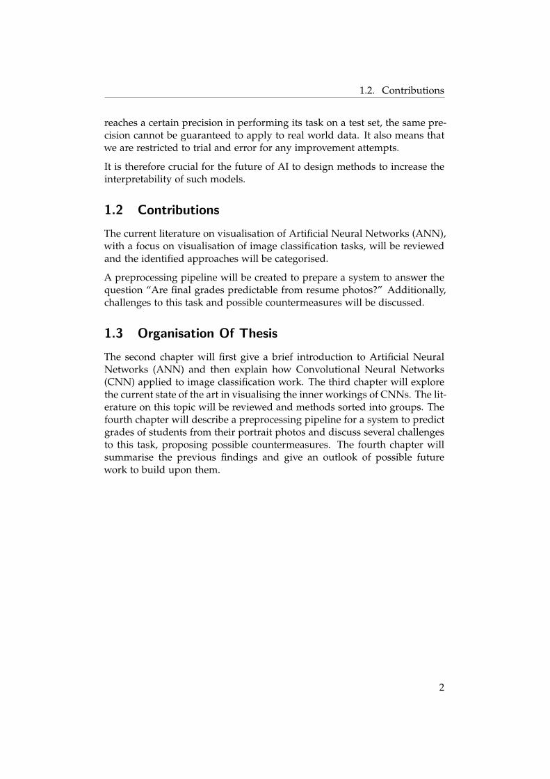
Figure 2.1: Diagram of artifical neuron or node in a NN with labelled components. Reprintedfrom [1]

Similar to neurons in brains, the basic unit of an ANN is an artifical neuron,also called node or unit. A neuron consists of several parts as shown in Fig.2.1. It receives a set of inputs, which are modified by a set of weights. Theweighted inputs are then passed into an activation function which computesthe output.

ANNs are composed of layers of neurons where the output of neurons inone layer are connected to the inputs of neurons in the next layer via adirected link. Layers where every neuron of one layer has a link to every

3

2.2. Convolutional Neural Networks

neuron in the next layer are called fully connected. These links propagate theactivation of a neuron to connected neurons in the next layer. Each of theselinks has an associated weight.

This way, data input to the network flows through each layer, finally emerg-ing from the last layer. This structure, where data only flows from input tooutput, is called a feed-forward network.

It is also possible to make connections from higher layers back to lower lay-ers. Networks with such backward connections are called Recurrent NeuralNetworks (RNN). Since this thesis is only concerned with feed-forward net-works, RNNs will not be expanded upon.

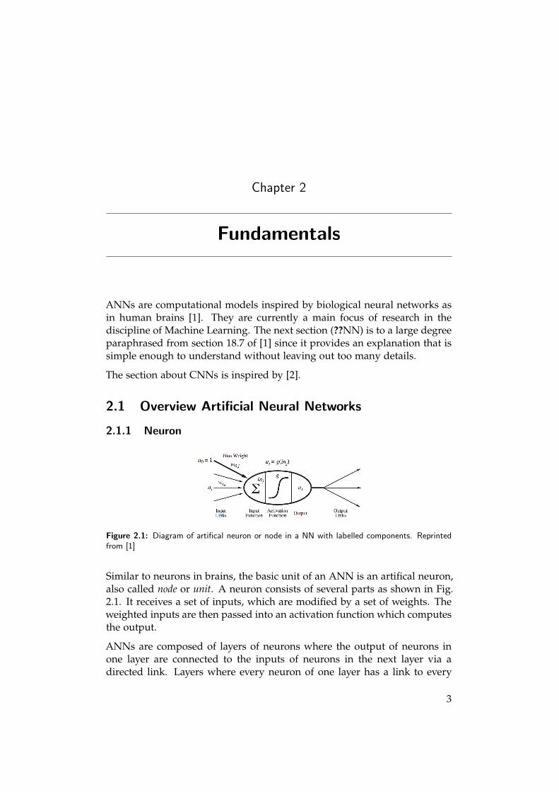
Figure 2.2: (a) A network with two input and two output neurons. (b) A network with twoinput neurons, two hidden neurons and two output neurons. Reprinted from [1]

2.1.2 Single-layer Networks

A single-layer network consists of a layer of input neurons connected toa layer of neurons, with the output of the network corresponding directlyto the output of the neurons (Fig. 2.2, (a)). The input layer performs nocomputation and just passes input it receives on to the next layer unchanged.In practice, this means each neuron in the output layer is a separate network,since its weights (which are essential to the learning process) only affect itsown output.

2.1.3 Multi-layer Networks

A multi-layer network is a layer of input neurons to which more than onelayer of neurons are connected (Fig. 2.2, (b)). Any layer between the inputand the last layer of neurons (output layer) is called a hidden layer, sincethey are not exposed to the outside.

Training of a multi-layer network is achieved by backpropagation of Errorsfrom the output layer. Before training, all weights in the network are initial-ized with random values. For every input fed to the network, the outputis compared with the desired output. The error is then propagated backthrough the network and weights are adjusted accordingly. This is repeateda fixed number of times or until the output error reaches a predeterminedthreshold.

4

2.2. Convolutional Neural Networks

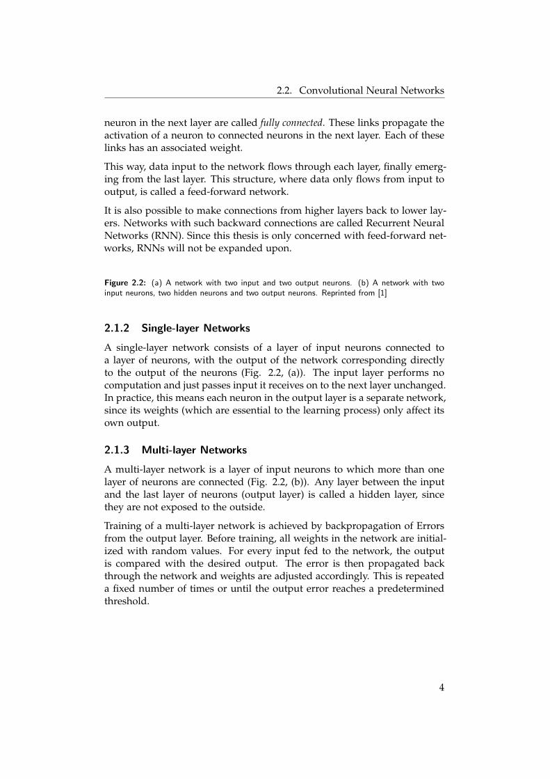
Figure 2.3: A simple CNN. Reprinted from [2]

2.2 Convolutional Neural Networks

Convolutional Neural Networks (CNN) are ANNs with a specific architec-ture. In recent years they have emerged as one of the most effective architec-tures for pattern recognition/feature extraction tasks. This thesis focuses onCNNs in the context of computer vision, specifically image classification, sothe CNN will be explained in this context. The input of a CNN for imageprocessing has 3 dimensions: height, width and depth (corresponding to thecolour channels of the image). CNN are generally composed of four mainoperations:

• Convolution

• Non-Linearity (ReLU)

• Pooling

• Classification (Fully Connected Layers)

Convolution, ReLU and pooling are usually combined to form a higher levelbuilding block. This block of layers can be repeated multiple times before anumber of fully connected layers is attached, with a final output layer withthe same number of outputs as expected classes.

2.2.1 Convolution

The convolution operation is a matrix operation, computing element wisemultiplication between two matrices and then adding the results to forma single integer. A convolution layer extracts features from the input bysliding a square matrix (called a filter) over the input image, performing theconvolution operation for each of its pixels.

To allow the outermost pixels of the image to be convolved, the image can bepadded with zeros on all sides. The result of applying a filter to the wholeinput is a new matrix with the results of each convolution. This is calleda feature map. Usually a convolution layer consists of more than one filter,each producing a feature map. The output of a convolution layer has thesame height and width as the input (if zero padding is used) and its depthcorresponds to the number of filters used.

5

2.2. Convolutional Neural Networks

2.2.2 ReLU

To introduce non-linearity into the CNN, a Rectified Linear Unit (ReLU) op-eration is performed after every convolutional layer. This basically replacesevery negative pixel value in the feature maps by zero. The ReLU operationis necessary because real-world data is usually non-linear and convolutionis a linear operation. Instead of ReLU, other non-linear functions like tanhor sigmoid can be used, but ReLU has shown the best performance for mostsituations.

2.2.3 Pooling

Spatial Pooling aggregates the values of several input pixels to a single out-put pixel, thereby reducing the size of each feature map. A feature map ofsize 4x4 can be reduced to an output of size 2x2. For this, a window of size2x2 is moved over the input, considering every pixel only once. The pixelsinside the window are aggregated, usually by selecting the maximum value.This is called Max Pooling.

The pooling step:

• reduces the size of the input representation, making it more manage-able

• reduces the number of parameters and thereby computations, control-ling overfitting and increasing performance

• increases resistance to small transformations, distortions and transla-tions

• renders the input representation almost scale invariant, meaning theobject to detect can be located anywhere in the input image

These three layer types differ from traditional multi-layer networks, as notevery neuron of a layer is connected to each neuron of the next layer.

2.2.4 Fully Connected Layers

Convolution, ReLU and Pooling layers together perform feature extraction,learning the most effective features for a given dataset. Every successiveblock of convolution, ReLU and pooling learns features on a higher levelthan the last, from edges up to complete objects. The highest level features(the output of the last convolution block) are then passed to a group of fullyconnected layers, where every neuron of each layer is connected to everyneuron in the next layer. The last fully connected layer finally correspondsdirectly to the class predictions, with each neurons output representing theprobability of one class.

6

2.2. Convolutional Neural Networks

2.2.5 Training

As with other ANNs, CNNs are trained using backpropagation, learningboth what features to extract and which classes the features or combinationsof features correspond to. Since feature extraction is mostly independent ofthe classification task, it is possible to freeze its parameters and only train aclassifier that uses the already learned features. This can significantly reducethe required size of the dataset needed for training, as long as the imagesthe feature extraction was trained with are similar to then new dataset.

7

Chapter 3

Literature Survey – Visualisation andUnderstanding of NN

There are several distinct ways to visualise what is happening inside of aneural network. The most obvious way is to graphically represent the struc-ture of the network. This can be used independently of the task, which alsomeans that it is difficult to gain insight into the processes involved in spe-cific tasks. The next section provides a short introduction to network visu-alisation with TensorFlow. After that, this thesis will focus on methods forvisualising image recognition and classification tasks, specifically for feedforward CNNs. [3] lists different analysis techniques. Two of those are con-cerned with visualisation: feature map reconstructions and input-featurebased model explanations. These correspond to what [4] calls feature vi-sualisation and attribution, respectively. Theses terms will be used in theremainder of this thesis.

3.1 Network Visualisation

Depending on the technology used, there are several tools available for thistask. For TensorFlow, the main tool available is TensorBoard.

A short overview of TensorBoard functionality is included, for in-depth ex-planation and code samples TensorFlow provides an excellent tutorial in itsdocumentation [5] and on the github repository of TensorBoard [6].

This shows a representation of the network as a graph of connected tensors(generally representing layers of the network as matrices of neurons thatform the layer) and their parameters. It also provides other tools to help un-derstand and debug TensorFlow programs, including dashboards for scalarvalues, plots of metrics and images that pass through the network. There arealso various add ons to enhance and add functionality. TensorBoard worksby reading the events file of TensorFlow runs. To create these event files,

8

3.1. Network Visualisation

the TensorFlow program needs to define data to be exposed to TensorBoardby adding summary operations to the TensorFlow code. A FileWriter thendumps these values and optionally the graph of a session to a event file. [6]

3.1.1 Graph Visualisation

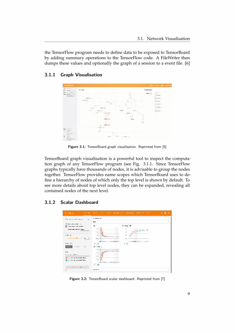
Figure 3.1: TensorBoard graph visualisation. Reprinted from [5]

TensorBoard graph visualisation is a powerful tool to inspect the computa-tion graph of any TensorFlow program (see Fig. 3.1.1. Since TensorFlowgraphs typically have thousands of nodes, it is advisable to group the nodestogether. TensorFlow provides name scopes which TensorBoard uses to de-fine a hierarchy of nodes of which only the top level is shown by default. Tosee more details about top level nodes, they can be expanded, revealing allcontained nodes of the next level.

3.1.2 Scalar Dashboard

Figure 3.2: TensorBoard scalar dashboard. Reprinted from [7]

9

3.2. Feature Visualisation

In the same way, summary operations can be defined to track scalar valueslike the model’s loss or learning rate. These values are then plotted as graphsto show their change over time and runs.

3.2 Feature Visualisation

The feature extraction part of a CNN is composed of various layers, theselayers each contain multiple feature detectors or filters. These filters arelearned by the network, not engineered. To understand how those filterslook and what kind or part of an input image activates a given filter, it is im-mensely helpful if they are visualised in some way. Understanding featureslearned by CNNs can be approached from two perspectives: visualisationof the response of the CNN to a specific input image and visualisation ofthe notion of a unit in the CNN[8]. [9] defines three different type of visual-isations: inversion, activation maximisation and caricaturisation. Inversionvisualises the response to a specific input, activation maximisation and car-icaturisation visualise the “meaning” of a component and combinations ofcomponents respectively. This section explores several different approachesfor each of these types.

The representation of the response to a specific image is created through dif-ferent backpropagation based approaches. Projecting the filter back to theinput pixel space from a feature map for a given image yields visual repre-sentations of the filters that created the map. While it is possible to projectfeature activations from the first convolutional layer back to the input pixelspace, the non-invertible nature of pooling operations requires a differentapproach for later layers.

The notion a network has of a class or unit is visualised by finding an in-put image that maximises activation. Another method is to optimise aninput image (or choose the optimal of multiple input images) for maximumactivation of different CNN components (neurons, channels, layers, classlogits/probabilities) and combinations of such components.

3.2.1 Inversion

Deconvolutional Networks (deconvnet)

[10] introduces a method to “map [feature activities in intermediate layers]back to the input pixel space” by attaching a deconvnet to each layer of theCNN Figure 3.3. This is one of the earliest approaches, it will be explainedmore in-depth than the rest. Most later approaches introduce improvementsbut are conceptually similar, so this will provide a good starting point.

First, an input image is fed into the CNN and features computed throughthe layers. To examine a given activation, all other activations in the layer

10

3.2. Feature Visualisation

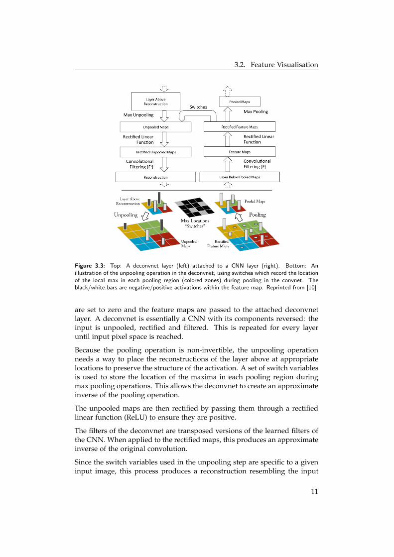
Figure 3.3: Top: A deconvnet layer (left) attached to a CNN layer (right). Bottom: Anillustration of the unpooling operation in the deconvnet, using switches which record the locationof the local max in each pooling region (colored zones) during pooling in the convnet. Theblack/white bars are negative/positive activations within the feature map. Reprinted from [10]

are set to zero and the feature maps are passed to the attached deconvnetlayer. A deconvnet is essentially a CNN with its components reversed: theinput is unpooled, rectified and filtered. This is repeated for every layeruntil input pixel space is reached.

Because the pooling operation is non-invertible, the unpooling operationneeds a way to place the reconstructions of the layer above at appropriatelocations to preserve the structure of the activation. A set of switch variablesis used to store the location of the maxima in each pooling region duringmax pooling operations. This allows the deconvnet to create an approximateinverse of the pooling operation.

The unpooled maps are then rectified by passing them through a rectifiedlinear function (ReLU) to ensure they are positive.

The filters of the deconvnet are transposed versions of the learned filters ofthe CNN. When applied to the rectified maps, this produces an approximateinverse of the original convolution.

Since the switch variables used in the unpooling step are specific to a giveninput image, this process produces a reconstruction resembling the input

11

3.2. Feature Visualisation

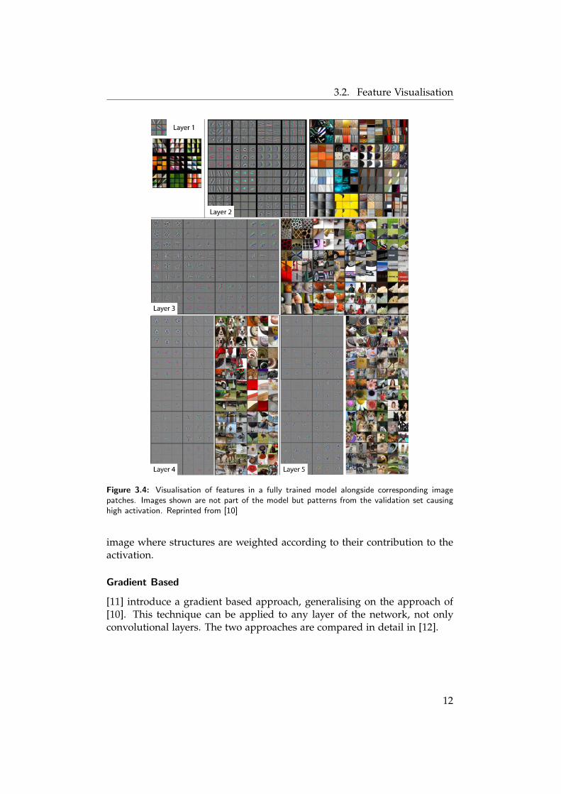
Figure 3.4: Visualisation of features in a fully trained model alongside corresponding imagepatches. Images shown are not part of the model but patterns from the validation set causinghigh activation. Reprinted from [10]

image where structures are weighted according to their contribution to theactivation.

Gradient Based

[11] introduce a gradient based approach, generalising on the approach of[10]. This technique can be applied to any layer of the network, not onlyconvolutional layers. The two approaches are compared in detail in [12].

12

3.2. Feature Visualisation

All-Convolutional Network and Guided Backpropagation

[13] introduces a CNN that replaces max pooling layers with convolutionallayers, removing the main impediment for backprojection of representationslearned by higher layers of a CNN. This allows for deconvolution withouta previous forward pass, since no switch variables are needed. In higherlayers, the deconvolution approach does not produce sharp, recognizableimages. To remedy this, [13] proposes a combination of [10] and [11], calledguided backpropagation, that significantly increases resulting image quality.

Guided Gradient-weighted Class Activation Mapping (Grad-CAM)

[14] introduces Grad-CAM, a generalisation to Class Activation Mapping(CAM) [15]. CAM/Grad-CAM is a localisation/attribution technique sec-tion 3.3. This technique is combined with guided backpropagation to re-move parts of the activation map that do not contribute to the final classifi-cation.

DeepLIFT

[16] introduces DeepLIFT, an approach that compares the difference of agiven output and a reference output with the difference of the inputs andreference inputs. Choosing a suitable reference to compare against is criticaland requires domain-specific knowledge.

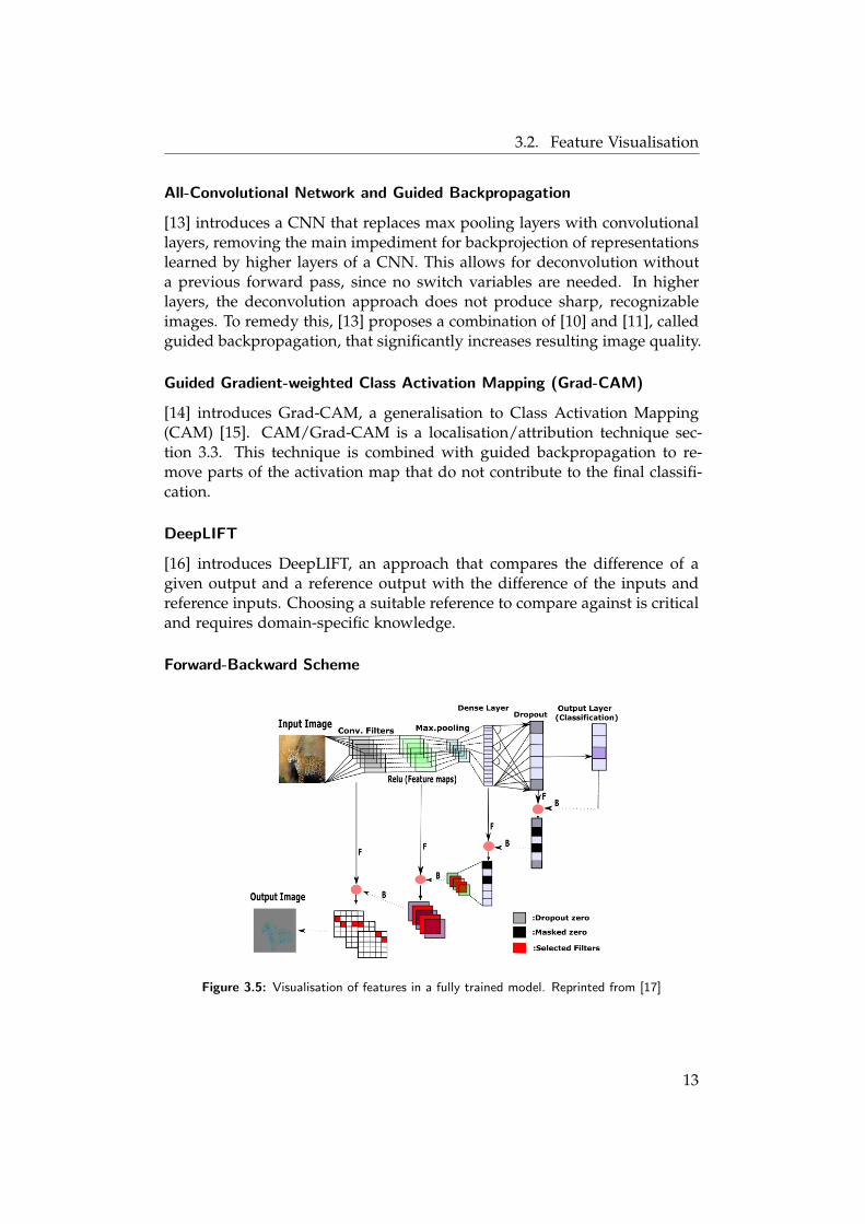
Forward-Backward Scheme

Figure 3.5: Visualisation of features in a fully trained model. Reprinted from [17]

13

3.2. Feature Visualisation

[17] introduces another alternative to the deconvnet back-propagation of[10], replacing it with a forward-backward scheme. It leverages both thebackward information flow during backpropagation from output layers toinput and the forward information flow during feature extraction. This ap-proach is computationally more efficient than [10] and does not have the po-tential numerical stability and robustness issues of gradient based schemeslike [13] and [14]. It also removes the need for a reference image as in [16].

Optimisation

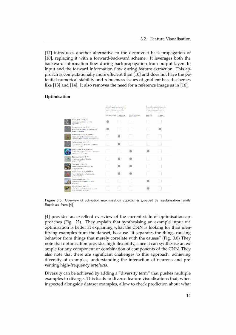
Figure 3.6: Overview of activation maximisation approaches grouped by regularisation family.Reprinted from [4]

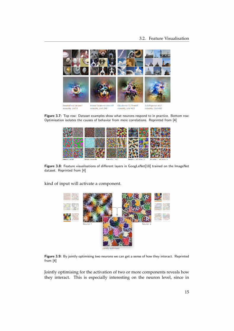
[4] provides an excellent overview of the current state of optimisation ap-proaches (Fig. ??). They explain that synthesising an example input viaoptimisation is better at explaining what the CNN is looking for than iden-tifying examples from the dataset, because “it separates the things causingbehavior from things that merely correlate with the causes” (Fig. 3.8) Theynote that optimisation provides high flexibility, since it can synthesise an ex-ample for any component or combination of components of the CNN. Theyalso note that there are significant challenges to this approach: achievingdiversity of examples, understanding the interaction of neurons and pre-venting high-frequency artefacts.

Diversity can be achieved by adding a “diversity term” that pushes multipleexamples to diverge. This leads to diverse feature visualisations that, wheninspected alongside dataset examples, allow to check prediction about what

14

3.2. Feature Visualisation

Figure 3.7: Top row: Dataset examples show what neurons respond to in practice. Bottom row:Optimisation isolates the causes of behavior from mere correlations. Reprinted from [4]

Figure 3.8: Feature visualisations of different layers in GoogLeNet[18] trained on the ImageNetdataset. Reprinted from [4]

kind of input will activate a component.

Figure 3.9: By jointly optimising two neurons we can get a sense of how they interact. Reprintedfrom [4]

Jointly optimising for the activation of two or more components reveals howthey interact. This is especially interesting on the neuron level, since in

15

3.2. Feature Visualisation

nature they work together to represent images.

Unfortunately, simply optimising an image to activate neurons producesimages with a high level of noise and high-frequency patterns. This has beenone of the top challenges in this and other feature visualisation approachesand most notable papers in this area contain some regularisation techniqueas a main point (Fig. 3.6.

A selection of different approaches from 3.6 is briefly explained below, start-ing with the core idea of activation maximisation.

Activation Maximisation

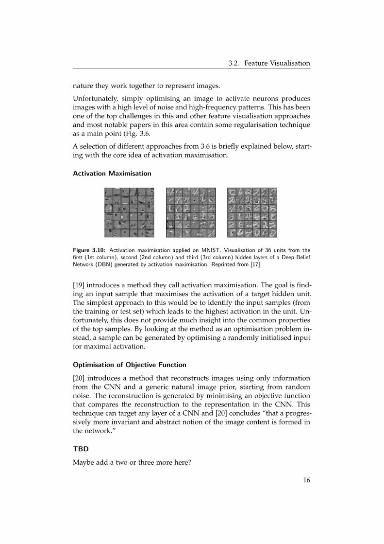
Figure 3.10: Activation maximisation applied on MNIST. Visualisation of 36 units from thefirst (1st column), second (2nd column) and third (3rd column) hidden layers of a Deep BeliefNetwork (DBN) generated by activation maximisation. Reprinted from [17]

[19] introduces a method they call activation maximisation. The goal is find-ing an input sample that maximises the activation of a target hidden unit.The simplest approach to this would be to identify the input samples (fromthe training or test set) which leads to the highest activation in the unit. Un-fortunately, this does not provide much insight into the common propertiesof the top samples. By looking at the method as an optimisation problem in-stead, a sample can be generated by optimising a randomly initialised inputfor maximal activation.

Optimisation of Objective Function

[20] introduces a method that reconstructs images using only informationfrom the CNN and a generic natural image prior, starting from randomnoise. The reconstruction is generated by minimising an objective functionthat compares the reconstruction to the representation in the CNN. Thistechnique can target any layer of a CNN and [20] concludes “that a progres-sively more invariant and abstract notion of the image content is formed inthe network.”

TBD

Maybe add a two or three more here?

16

3.3. Attribution

3.2.2 Caricaturisation

Caricaturisation is a variant of Optimisation where instead of a randominput, an initial image is modified by optimisation to enhance any patternthat triggers activation[9].

3.3 Attribution

Attribution has the goal to identify and highlight the parts of an input thatcontribute most to the final classification. It is closely related to object local-isation in scenes.

Two types of visualisation are employed for attribution in computer vision[3]:

• Correct class heat maps: A heat map is overlaid or opacity reducedon the input image according to the encoded probability of the correctclass. This shows which superpixels are important.

• Most-likely class image Each superpixel in the original image is colouredaccording to its most likely class.

Occlusion Sensitivity Analysis

[10] describes a method to identify the contribution of superpixels or regionsof the input image by successively occluding part of the image by a graysquare and running the classifier on the occluded image. Each occludedpart is then coloured according to the class probabilities of the occludedimage.

Class Activation Maps (CAM)

[15] introduces CAM, a method using global average pooling to identify thediscriminative image regions used by the CNN for classification.

17

Chapter 4

Towards an Experimental Testbed forDebugging NN

4.1 Data

In the bachelors degree programme in Computer Science (BA in CS) atZurich University of Applied Sciences (ZHAW), the first two semesters (threesemesters for part-time students) form the assessment level. An averagegrade of 4.0 or higher in all modules is the requirement for admission to themain study programme.

A dataset of portraits of both current and former students the BA in CSat ZHAW and their respective average grade for the assessment level wasprovided by the school. For privacy reasons, no names or other identifyinginformation was included. Additionally this ensured that no other informa-tion could be used by the network for classification.

4.1.1 Challenges

The dataset contains data for 430 students, which is an extremely low num-ber for training a CNN. Standard training datasets for specific types of im-ages like Labelled Faces in the Wild (LFW) [?] contain over ten thousandimages, others like ImageNet [?] even contain Millions. Two approaches areproposed to alleviate the impact of the small number of images. First, DataAugmentation can been integrated into the learning process by randomlytransforming the images, thus producing several versions of each image.Second, a network model that has already been trained on a large dataset offaces and has thus learned relevant features can be used as a basis. On topof that model, a number of fully connected layers can be trained to classifyimages using the features from the pre-trained model.

Another challenge is the class imbalance in the dataset when using pass/fail

18

4.2. Preprocessing

as classes. Since most students have so far passed the assessment with onlya few failing to do so (about 400 passing and 30 failing), a CNN couldachieve over 90% accuracy by simply classifying all images in a test datasetthat has the same distribution of classes as pass. This can be alleviated bymoving the “pivot point” from 4.0 to 4.75, which is the median of gradesover all students. A second approach to fix the class imbalance issue wouldbe to adjust the loss function to account for the imbalance and punish falsenegatives in addition to rewarding true positives. Several other methods toaddress imbalance are surveyed in [?].

4.2 Preprocessing

The data was provided as an Excel file containing the image, grade and anumerical identifier.

4.2.1 Extraction from Excel file

To simplify working with the images, a Python script was developed toextract the images from the Excel file and store them in a directory. Addi-tionally, a CSV file with the file name and grade for a student in each rowwas created for assigning each student to a class for training and validation.

4.2.2 Cropping Faces

For use in training a CNN, all input images need to have the same size.Most network architectures also expect the input to have a square shape. APython script was written to automate this task. To identify the face andcentre the crop region on it, OpenCV was used. For each image, the scriptfirst locates the face and crops away its surroundings. The face is then savedto a separate folder, resizing it to 160x160 pixels in the process.

4.2.3 Sorting Faces by Class Membership

To assign images to a class a script was developed to sort them into directo-ries corresponding to correct class labels. This was done to prepare the datato be read by Keras [?], which was chosen as the framework to build theCNN with. Keras provides methods to read training and test data from thistype of stucture and automatically extract and assign the correct class labelfor each image.

4.3 Proof of Concept

A first small proof of concept CNN (POC) was built using Keras to demon-strate that the data is suitable to be used for training after these preprocess-

19

4.3. Proof of Concept

ing steps. Input images were grouped into the two classes pass (grade ¿=4.0) and fail (grade ¡ 4.0) and the POC was trained with this data.

20

Chapter 5

Summary and Future Work

After establishing that interpretability is key for reliability, especially in crit-ical applications, an overview of the current state of the art methods forenhancing the interpretability of CNNs was provided. Even consideringthat the overview focussed on methods compatible with CNNs and specif-ically the visualisation of image classification tasks, many of the exploredapproaches are applicable to other domains and architectures. The wealthof methods and approaches shows that the view of ANNs as a inscrutableblack boxes is at best outdated. There still is much room for deeper under-standing of the inner workings of ANNs, but we already have a lot of toolsto support us in this challenge.

A preprocessing pipeline has been created to support future experimentalexploration of the question “Are final grades predictable from resume pho-tos?” Additionally, several challenges to this task have been identified, formost of which countermeasures have been proposed.

The next step would be combining these results to build a system for train-ing, evaluating and visualise image classification tasks. For this, a pre-trained model needs to be chosen and, if necessary, adapted to ensure com-patibility with different visualisation techniques.

21

Bibliography

[1] S. Russell and P. Norvig, “Artificial Intelligence A Modern Approach,2nd edn,” 2003.

[2] U. Karn, “An Intuitive Explanation of Convolutional NeuralNetworks.” [Online]. Available: https://ujjwalkarn.me/2016/08/11/intuitive-explanation-convnets/

[3] M. Thoma, “Analysis and Optimization of Convolutional NeuralNetwork Architectures,” jul 2017. [Online]. Available: http://arxiv.org/abs/1707.09725

[4] C. Olah, A. Mordvintsev, and L. Schubert, “Feature Visualization,”Distill, vol. 2, no. 11, p. e7, nov 2017. [Online]. Available:https://distill.pub/2017/feature-visualization

[5] “TensorBoard: Visualizing Learning.” [Online]. Available: https://www.tensorflow.org/get started/summaries and tensorboard

[6] “Tensorboard Github.” [Online]. Available: https://github.com/tensorflow/tensorboard

[7] “Edward - Tensorboard.” [Online]. Available: http://edwardlib.org/tutorials/tensorboard

[8] L. M. Zintgraf, T. S. Cohen, and M. Welling, “A New Methodto Visualize Deep Neural Networks,” mar 2016. [Online]. Available:http://arxiv.org/abs/1603.02518

[9] A. Mahendran and A. Vedaldi, “Visualizing Deep Convo-lutional Neural Networks Using Natural Pre-Images,” dec2015. [Online]. Available: http://arxiv.org/abs/1512.02017http://dx.doi.org/10.1007/s11263-016-0911-8

22

Bibliography

[10] M. D. Zeiler and R. Fergus, “Visualizing and Understanding Con-volutional Networks.” Springer, Cham, 2014, pp. 818–833. [Online].Available: http://link.springer.com/10.1007/978-3-319-10590-1 53

[11] K. Simonyan, A. Vedaldi, and A. Zisserman, “Deep InsideConvolutional Networks: Visualising Image Classification Models andSaliency Maps,” dec 2013. [Online]. Available: http://arxiv.org/abs/1312.6034

[12] A. Mahendran and A. Vedaldi, “Salient Deconvolutional Networks.”Springer, Cham, oct 2016, pp. 120–135. [Online]. Available: http://link.springer.com/10.1007/978-3-319-46466-4 8

[13] J. T. Springenberg, A. Dosovitskiy, T. Brox, and M. Riedmiller, “Strivingfor Simplicity: The All Convolutional Net,” dec 2014. [Online].Available: http://arxiv.org/abs/1412.6806

[14] R. R. Selvaraju, M. Cogswell, A. Das, R. Vedantam, D. Parikh, andD. Batra, “Grad-CAM: Visual Explanations from Deep Networksvia Gradient-based Localization,” oct 2016. [Online]. Available:http://arxiv.org/abs/1610.02391

[15] B. Zhou, A. Khosla, A. Lapedriza, A. Oliva, and A. Torralba, “LearningDeep Features for Discriminative Localization,” dec 2015. [Online].Available: http://arxiv.org/abs/1512.04150

[16] A. Shrikumar, P. Greenside, and A. Kundaje, “Learning ImportantFeatures Through Propagating Activation Differences,” apr 2017.[Online]. Available: http://arxiv.org/abs/1704.02685

[17] A. Balu, T. V. Nguyen, A. Kokate, C. Hegde, and S. Sarkar, “AForward-Backward Approach for Visualizing Information Flow inDeep Networks,” nov 2017. [Online]. Available: http://arxiv.org/abs/1711.06221

[18] C. Szegedy, W. Liu, Y. Jia, P. Sermanet, S. Reed, D. Anguelov, D. Erhan,V. Vanhoucke, and A. Rabinovich, “Going Deeper with Convolutions,”sep 2014. [Online]. Available: http://arxiv.org/abs/1409.4842

[19] D. Erhan, Y. Bengio, A. Courville, and P. Vin-cent, “Visualizing higher-layer features of a deep net-work,” Bernoulli, no. 1341, pp. 1–13, 2009. [Online]. Avail-able: http://igva2012.wikispaces.asu.edu/file/view/Erhan+2009+Visualizing+higher+layer+features+of+a+deep+network.pdf

23

[20] A. Mahendran and A. Vedaldi, “Understanding Deep ImageRepresentations by Inverting Them,” nov 2014. [Online]. Available:http://arxiv.org/abs/1412.0035

[21] “Labelled Faces in the Wild.”

[22] “ImageNet.”

[23] M. Buda, A. Maki, and M. A. Mazurowski, “A systematic study of theclass imbalance problem in convolutional neural networks,” oct 2017.[Online]. Available: http://arxiv.org/abs/1710.05381

[24] “Keras.” [Online]. Available: https://keras.io/

List of Figures

2.1 Diagram of artifical neuron or node in a NN with labelled com-ponents. Reprinted from [1] . . . . . . . . . . . . . . . . . . . . . . 3

2.2 (a) A network with two input and two output neurons. (b) Anetwork with two input neurons, two hidden neurons and twooutput neurons. Reprinted from [1] . . . . . . . . . . . . . . . . . 4

2.3 A simple CNN. Reprinted from [2] . . . . . . . . . . . . . . . . . . 5

3.1 TensorBoard graph visualisation. . . . . . . . . . . . . . . . . . . . 93.2 TensorBoard scalar dashboard. . . . . . . . . . . . . . . . . . . . . 93.3 Top: A deconvnet layer (left) attached to a CNN layer (right).

Bottom: An illustration of the unpooling operation in the de-convnet, using switches which record the location of the localmax in each pooling region (colored zones) during pooling in theconvnet. The black/white bars are negative/positive activationswithin the feature map. Reprinted from [10] . . . . . . . . . . . . 11

3.4 Visualisation of features in a fully trained model alongside cor-responding image patches. Images shown are not part of themodel but patterns from the validation set causing high activa-tion. Reprinted from [10] . . . . . . . . . . . . . . . . . . . . . . . . 12

24

List of Figures

3.5 Visualisation of features in a fully trained model. Reprinted from[17] . . . . . . . . . . . . . . . . . . . . . . . . . . . . . . . . . . . . 13

3.6 Overview of activation maximisation approaches grouped by reg-ularisation family. Reprinted from [4] . . . . . . . . . . . . . . . . 14

3.7 Top row: Dataset examples show what neurons respond to inpractice. Bottom row: Optimisation isolates the causes of behav-ior from mere correlations. Reprinted from [4] . . . . . . . . . . . 15

3.8 Feature visualisations of different layers in GoogLeNet[18] trainedon the ImageNet dataset. Reprinted from [4] . . . . . . . . . . . . 15

3.9 By jointly optimising two neurons we can get a sense of how theyinteract. Reprinted from [4] . . . . . . . . . . . . . . . . . . . . . . 15

3.10 Activation maximisation applied on MNIST. Visualisation of 36units from the first (1st column), second (2nd column) and third(3rd column) hidden layers of a Deep Belief Network (DBN) gen-erated by activation maximisation. Reprinted from [17] . . . . . . 16

25

Appendix A

Code Listings and Dataset

Scripts for the preprocessing pipeline and the training data are provided onan external storage medium and will be handed in with the print version ofthis thesis.

26

Zürcher Fachhochschule

Erklärung betreffend das selbständige Verfassen einer Projektarbeit an der School of Engineering

Mit der Abgabe dieser Projektarbeit versichert der/die Studierende, dass er/sie die Arbeit selbständig und ohne fremde Hilfe verfasst hat. (Bei Gruppenarbeiten gelten die Leistungen der übrigen Gruppen-mitglieder nicht als fremde Hilfe.)

Der/die unterzeichnende Studierende erklärt, dass alle zitierten Quellen (auch Internetseiten) im Text oder Anhang korrekt nachgewiesen sind, d.h. dass die Projektarbeit keine Plagiate enthält, also keine Teile, die teilweise oder vollständig aus einem fremden Text oder einer fremden Arbeit unter Vorgabe der eigenen Urheberschaft bzw. ohne Quellenangabe übernommen worden sind. Bei Verfehlungen aller Art treten die Paragraphen 39 und 40 (Unredlichkeit und Verfahren bei Unredlichkeit) der ZHAW Prüfungsordnung sowie die Bestimmungen der Disziplinarmassnahmen der Hochschulordnung in Kraft.

Ort, Datum: Unterschriften:

……………………………………………… ……………………………………………………………

…………………………………………………………...

……………………………………………………………

Das Original dieses Formulars ist bei der ZHAW-Version aller abgegebenen Projektarbeiten zu Beginn der Dokumentation nach dem Titelblatt mit Original-Unterschriften und -Datum (keine Kopie) einzufügen.