Decision Making in Kidney Paired Donation Programswith Altruistic Donors ∗

Yijiang Li, Peter X.-K. Song, Alan B. Leichtman,Michael A. Rees, and John D. Kalbfleisch

Abstract

In recent years, kidney paired donation (KPD) has been extended to include livingnon-directed or altruistic donors, in which an altruistic donor donates to the candidateof an incompatible donor-candidate pair with the understanding that the donor in thatpair will further donate to the candidate of a second pair, and so on; such a processcontinues and thus forms an altruistic donor-initiated chain. In this paper, we proposea novel strategy to sequentially allocate the altruistic donor (or bridge donor) so asto maximize the expected utility; analogous to the way a computer plays chess, theidea is to evaluate different allocations for each altruistic donor (or bridge donor) bylooking several moves ahead in a derived look-ahead search tree. Simulation studiesare provided to illustrate and evaluate our proposed method.

KEY WORDS: Altruistic donors; decision analysis; kidney paired donation; look-aheadsearch tree.MSC2000 CLASSIFICATION: 62 - Statistics; 90 - Operations Research, MathematicalProgramming

∗Yijiang Li is Statistician at Google Inc., Mountain View, CA 94043, (Email: yijiang1121@gmail.com),John D. Kalbfleisch is Professor (Email: jdkalbfl@umich.edu), Peter X.-K. Song is Professor (Email: px-song@umich.edu), Department of Biostatistics, University of Michigan, Ann Arbor, MI 48109. Alan B. Le-ichtman is Professor, Department of Internal Medicine, University of Michigan, Ann Arbor, MI 48109 (Email:aleicht@med.umich.edu). Michael A. Rees is Professor, Department of Urology, University of Toledo MedicalCenter, Toledo, Ohio 43614 (Email: michael.rees2@utoledo.edu).

1

1 Introduction

For patients with end stage renal disease (ESRD), kidney transplantation is a preferred

treatment as compared with dialysis for it provides not only a longer survival but also a

better quality of life (Evans et al. 1985, Russell et al. 1992, Wolfe et al. 1999). According

to the Organ Procurement and Transplantation Network (OPTN), about 16, 760 kidney

transplants were performed per year from 2009 to 2012 in the U.S., while during that same

period of time the yearly average number of patients added to the waiting list for kidney

transplant surpassed 34, 100. Part of this gap between supply and demand can be attributed

to the unfortunate fact that many patients with kidney failure recruit willing organ donors

who, upon evaluation, prove to be ABO blood type and/or Human Leukocyte Antigens

(HLA) incompatible. With regard to blood type compatibility, A and B donors can donate

to candidates of the same blood type or of type AB; AB donors can donate only to AB

candidates; and O donors, known as universal donors, can donate to candidates of any blood

type. The HLA incompatibility, on the other hand, is due to the candidate having antibodies

against the HLA antigens of a potential donor resulting from prior exposure to donor antigens

through pregnancy, transfusion or previous transplant. Both forms of incompatibility can

lead to a rapid rejection of the transplanted organ and thus prohibit transplantation.

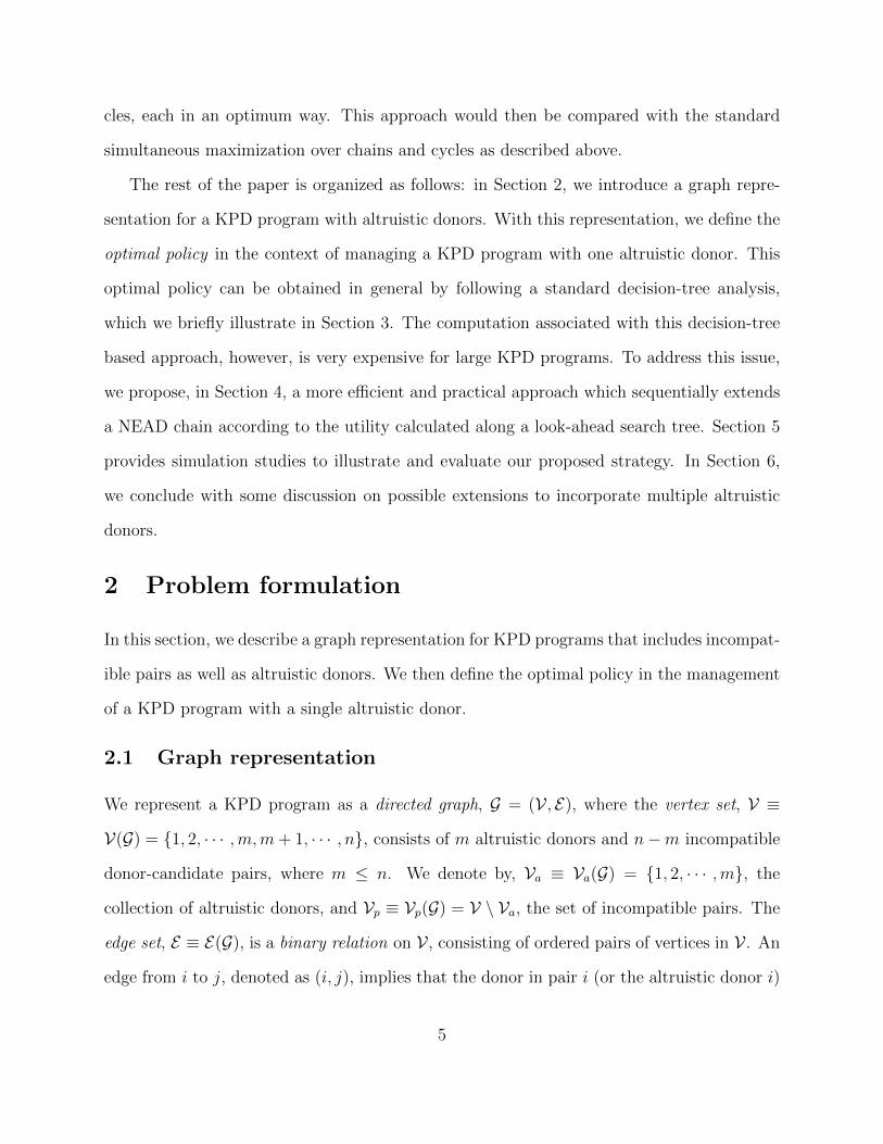
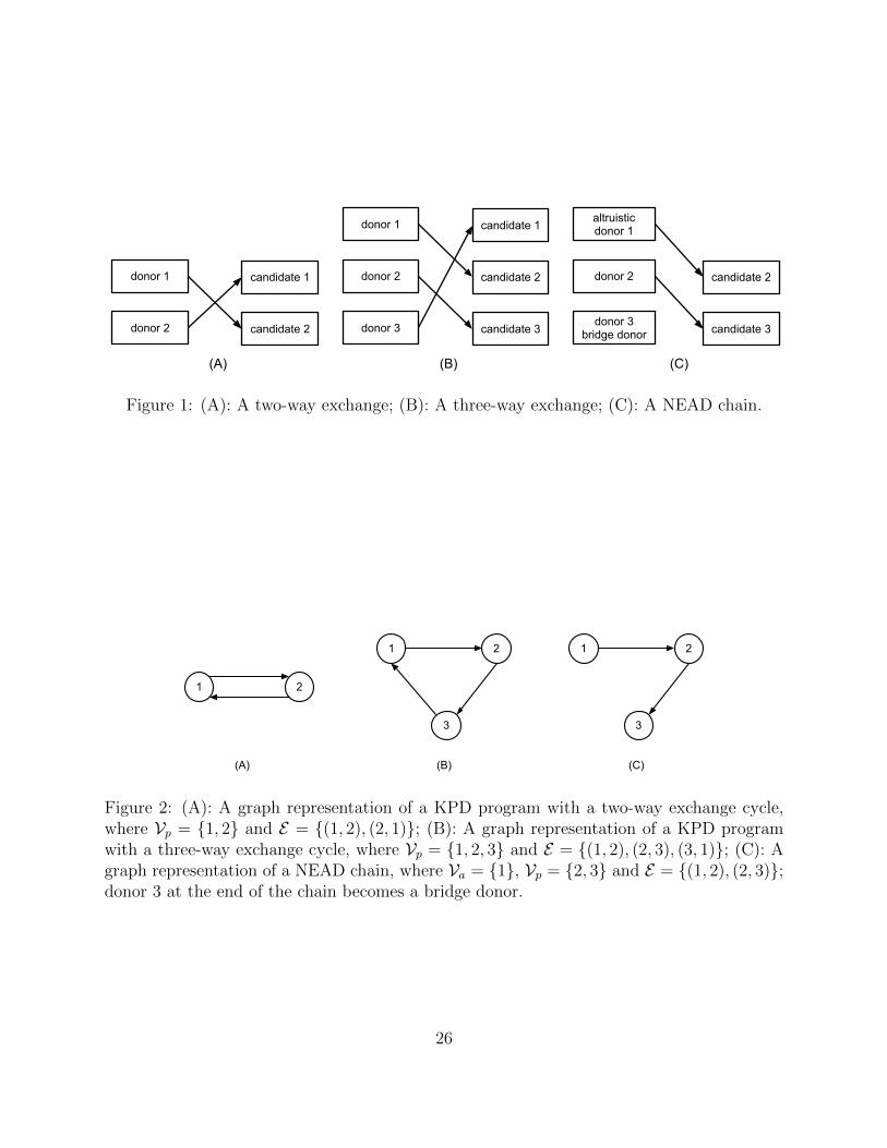
An evolving strategy, known as kidney paired donation (KPD) (Rapaport 1986) matches

one donor-candidate pair to another pair with a complementary incompatibility, such that the

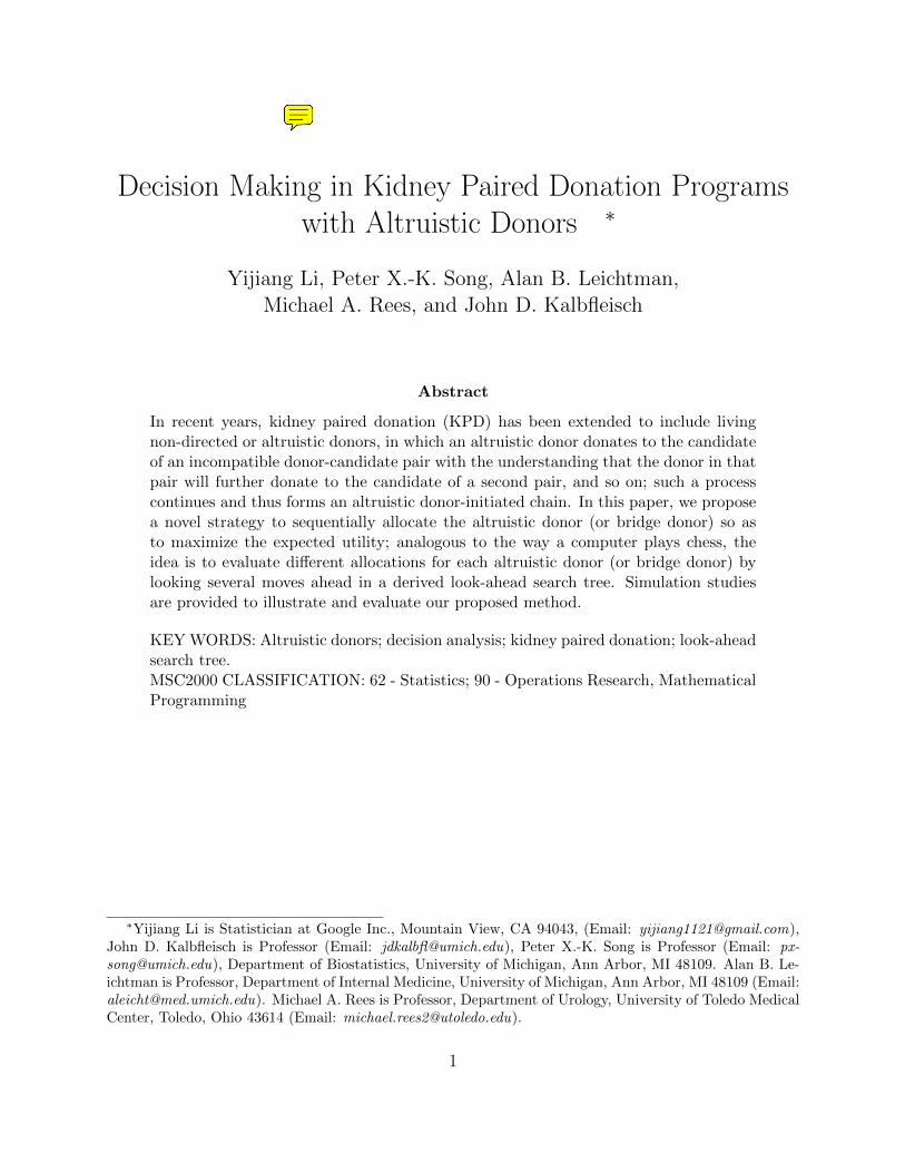
donor of the first pair donates to the candidate of the second, and vice versa; see Figure 1-A

and Figure 1-B for illustrations of a two-way exchange and a three-way exchange. Although

three-way or higher exchange cycles increase the chance of identifying compatible matches,

most KPD programs restrict exchanges to at most three ways for two primary reasons. First,

all surgical operations in a cycle must be performed simultaneously to avoid the possibility

that one of the donors may renege. This requirement creates substantial logistical difficulties

2

of scheduling, for example, eight surgeons and eight operating rooms at the same time for a

four-way exchange. Second, the greater the length of an exchange cycle, the less likely the

potential transplants involved will actually occur, for the whole exchange cycle collapses if

any of the proposed transplants cannot proceed.

[Figure 1 here]

A fundamental problem in managing KPD programs lies in selecting the “optimal” set of

kidney exchanges from among the many possible alternatives. This problem has been mod-

eled and analyzed by economists using a game-theoretic approach (Roth et al. 2004). More

general approaches have been developed to tackle such a problem via an integer programming

(IP) formulation, first proposed by Roth et al. (2007); In this, each potential transplant was

assigned equal weight, resulting in an allocation strategy that enables the greatest number

of transplants to be potentially implemented. Abraham et al. (2007) adopted a more flexible

weight assignment in this IP-based formulation and further developed an algorithm to reduce

the computational complexity of managing large KPD programs. Li et al. (2013) considered

a general utility-based evaluation of potential kidney transplants. Moreover, they explicitly

took into account inherent uncertainties in managing KPD programs and exploited possible

fall-back or contingent exchanges when the originally planned allocation cannot be fully ex-

ecuted. In a data-driven simulation system, they demonstrate that taking such additional

elements into consideration would yield improved allocation strategies.

In recent years, KPD has also been extended to include living non-directed donors

(LNDs), or altruistic donors; these are donors who have no designated candidates and decide

to donate voluntarily to a stranger. In this context, an altruistic donor may donate to the

candidate of an incompatible pair with the understanding that the donor of that pair will

become a bridge donor, and further donate to the candidate of a second pair, and so on;

such a process continues and thus forms an LND-initiated chain. One advantage to such

chains as compared to two-way or higher order exchange cycles is that transplants along

3

the chain do not need to be performed simultaneously (Montgomery et al. 2006, Roth et al.

2006). As a consequence, the donor whose incompatible candidate has received another

donor’s kidney but has yet to donate could donate later to another candidate; such donors

are hence called “bridge donors”. For this reason, this LND-initiated chain is sometimes

called a non-simultaneous extended altruistic donor (NEAD) chain (Rees et al. 2009). Fig-

ure 1-C illustrates a NEAD chain. Kidneys from altruistic donors used to be designated

to patients with no living donors and who have therefore been placed on a deceased-donor

waiting list. A NEAD chain, however, allows for passing the altruism beyond saving just one

patient, to potentially benefitting several patients in the chain; the final donor in an NEAD

chain could still donate to the deceased-donor waiting list. The advantage of such chains has

already been demonstrated via simulation studies by Gentry et al. (2009) and Ashlagi et al.

(2011). In clinical practice, the standard way of incorporating LND and bridge donors into

the optimization of a KPD is to consider chains up to a given length along with cycles in the

optimization for each match run. Thus, at regular intervals, the KPD pool is examined and

a set of chains segments and/or a set of cycles are chosen using the integer programming

approach, and those chosen are implemented if possible.

In this paper, we consider a different strategy for developing a NEAD chain under uncer-

tainties in a KPD program with one altruistic donor. We also discuss in general some possible

extensions of this strategy to incorporate multiple altruistic donors. Analogous to the way a

computer plays chess, we propose an approach to sequentially allocating an altruistic donor

(or a bridge donor) so as to maximize the expected utility over a certain given number of

moves. The idea is to evaluate different allocation options available for each altruistic donor

(or bridge donor) by looking several moves ahead along a derived look-ahead search tree.

With these options in mind, we proceed with the next allocation of the altruistic or bridge

donor that has the highest evaluation. This is the first step in developing an approach that

would alternate between optimizing the use of LND and bridge donors and assigning cy-

4

cles, each in an optimum way. This approach would then be compared with the standard

simultaneous maximization over chains and cycles as described above.

The rest of the paper is organized as follows: in Section 2, we introduce a graph repre-

sentation for a KPD program with altruistic donors. With this representation, we define the

optimal policy in the context of managing a KPD program with one altruistic donor. This

optimal policy can be obtained in general by following a standard decision-tree analysis,

which we briefly illustrate in Section 3. The computation associated with this decision-tree

based approach, however, is very expensive for large KPD programs. To address this issue,

we propose, in Section 4, a more efficient and practical approach which sequentially extends

a NEAD chain according to the utility calculated along a look-ahead search tree. Section 5

provides simulation studies to illustrate and evaluate our proposed strategy. In Section 6,

we conclude with some discussion on possible extensions to incorporate multiple altruistic

donors.

2 Problem formulation

In this section, we describe a graph representation for KPD programs that includes incompat-

ible pairs as well as altruistic donors. We then define the optimal policy in the management

of a KPD program with a single altruistic donor.

2.1 Graph representation

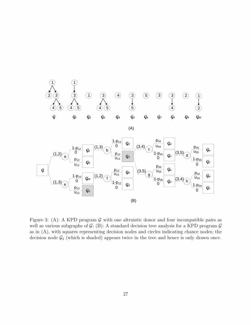
We represent a KPD program as a directed graph, G = (V , E), where the vertex set, V ≡

V(G) = {1, 2, · · · ,m,m + 1, · · · , n}, consists of m altruistic donors and n−m incompatible

donor-candidate pairs, where m ≤ n. We denote by, Va ≡ Va(G) = {1, 2, · · · ,m}, the

collection of altruistic donors, and Vp ≡ Vp(G) = V \ Va, the set of incompatible pairs. The

edge set, E ≡ E(G), is a binary relation on V , consisting of ordered pairs of vertices in V . An

edge from i to j, denoted as (i, j), implies that the donor in pair i (or the altruistic donor i)

5

is predicted to be compatible with the candidate in pair j. Such a prediction is based on a

virtual crossmatch test, which involves computer cross-checking for blood type compatibility

as well as comparing preexisting candidate antibodies against donor HLA antigens. Before a

predicted compatible transplant can be further considered for an actual surgical operation,

the compatibility must be confirmed by a more labor-intensive laboratory crossmatch test to

assure histocompatibility; this involves incubating the serum of a candidate with the white

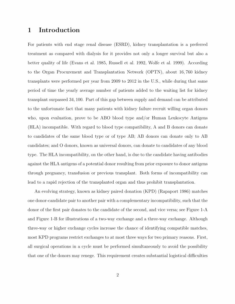
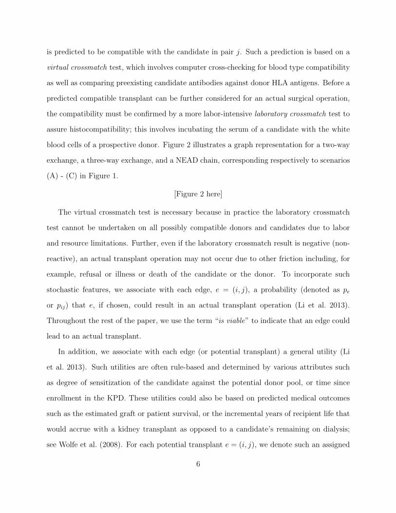
blood cells of a prospective donor. Figure 2 illustrates a graph representation for a two-way

exchange, a three-way exchange, and a NEAD chain, corresponding respectively to scenarios

(A) - (C) in Figure 1.

[Figure 2 here]

The virtual crossmatch test is necessary because in practice the laboratory crossmatch

test cannot be undertaken on all possibly compatible donors and candidates due to labor

and resource limitations. Further, even if the laboratory crossmatch result is negative (non-

reactive), an actual transplant operation may not occur due to other friction including, for

example, refusal or illness or death of the candidate or the donor. To incorporate such

stochastic features, we associate with each edge, e = (i, j), a probability (denoted as pe

or pij) that e, if chosen, could result in an actual transplant operation (Li et al. 2013).

Throughout the rest of the paper, we use the term “is viable” to indicate that an edge could

lead to an actual transplant.

In addition, we associate with each edge (or potential transplant) a general utility (Li

et al. 2013). Such utilities are often rule-based and determined by various attributes such

as degree of sensitization of the candidate against the potential donor pool, or time since

enrollment in the KPD. These utilities could also be based on predicted medical outcomes

such as the estimated graft or patient survival, or the incremental years of recipient life that

would accrue with a kidney transplant as opposed to a candidate’s remaining on dialysis;

see Wolfe et al. (2008). For each potential transplant e = (i, j), we denote such an assigned

6

utility as ue or uij.

In this paper, our attention is not on the estimation of edge utilities and probabilities. It

is worth noting though that research along this line is important and needed in the practical

management of a KPD program; see more discussion on this aspect in Wolfe et al. (2008),

Schaubel et al. (2009), and Li et al. (2013).

2.2 The optimal policy

One difficulty with selecting a long NEAD chain and then arranging transplants accordingly

is that in practice this long chain can rarely be fully implemented. This is because the

chain would break as soon as one transplant cannot proceed as planned. In this paper,

we propose to extend a NEAD chain sequentially in a near optimal way by selecting one

potential transplant recipient at a time. In subsequent discussion, we note how this can be

used as the basis of more general approaches.

Consider a KPD program with only one altruistic donor, i.e. m = 1 and Va = {1}.

This naturally implies (i, 1) /∈ E for all i ∈ V , as altruistic donors don’t have designated

candidates. For j ∈ V such that j = 1 or (1, j) ∈ E , let G(j) ≡ (Vj, Ej) be a subgraph of

G = (V , E), where

Vj = {v ∈ V : v is accessible from j},

Ej = {(v1, v2) ∈ E : v1 ∈ Vj, v2 ∈ Vj, v2 6= j}.

In this paper, a vertex j is said to be accessible from a vertex i if i = j or if there exists

a set of edges in E , denoted as {(ik, ik+1), k = 0, 1, · · · , n} such that i0 = i and in+1 = j.

In general terms, G(j) represents the resulting KPD graph if the transplant according to

(1, j) ∈ E is arranged and j becomes a bridge donor.

Managing a KPD program with one altruistic donor could then be viewed as a sequential

decision problem, in which we start with U = 0 and G = G(1), and then repeat the following

steps until |V(G)| = 1:

7

(i) choose one edge from A ≡ {(1, j) : (1, j) ∈ E}, say (1, b).

(ii) if (1, b) is viable, update

U ← U + u1b,

G ← G(b),

1← b;

if (1, b) is not viable, update the KPD pool

G ← G−b(1), where G−b = (V , E \ {(1, b)}) .

Step (i) is carried out to implement a policy that would be used to manage the KPD

program by specifying what action from A to take at each loop; two sample policies are,

b = argmaxj:(1,j)∈A

u1j

b = argmaxj:(1,j)∈A

u1jp1j.

These correspond to greedy algorithms that look at the next step only and manage to

optimize the utility or the expected utility of that step. They may, of course, be very poor

strategies since they ignore any subsequent implications of possible next steps.

For any given policy on G = (V , E), the value of U after the algorithm terminates can

be interpreted as the cumulative claimed utility. This value, which we denote by U∞, is

random; and its expectation could be used to evaluate the policy from which it arose. Among

all policies defined in the above way, the optimal policy refers to the one that attains the

highest value of E(U∞). This way of defining the optimal policy provides a formal framework

that will prove convenient in later discussions, even though in general one can rarely follow

this optimal policy through until the iterative procedure ends. This is an important issue,

arising due to various practical concerns, that we will revisit in Section 4.2.

8

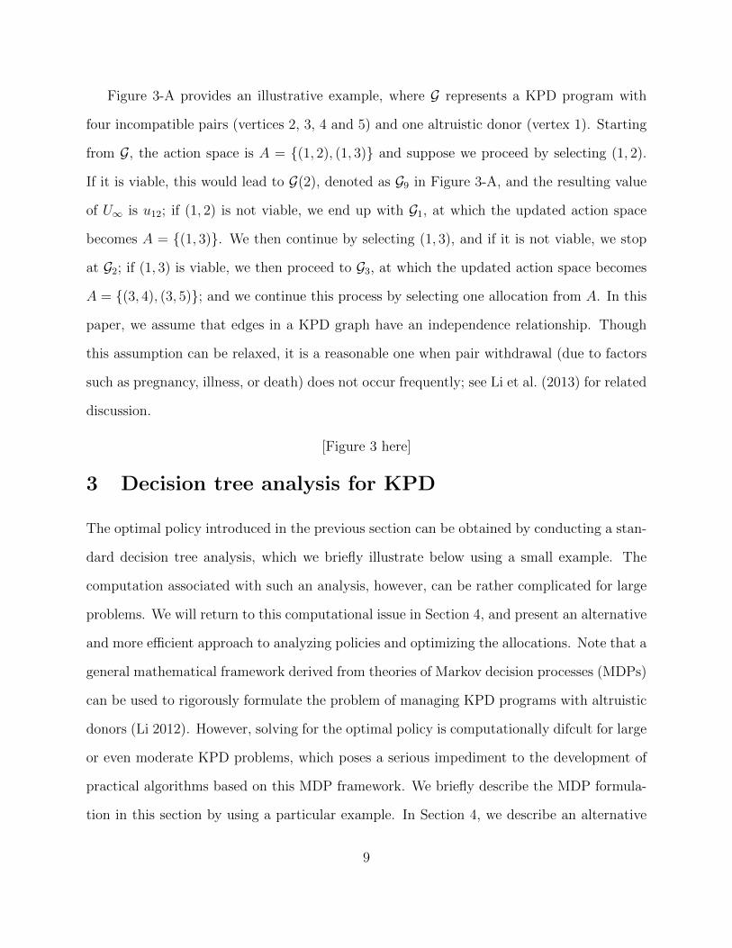
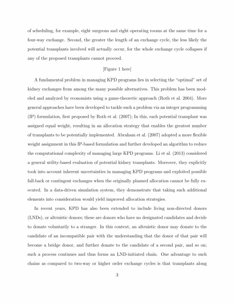
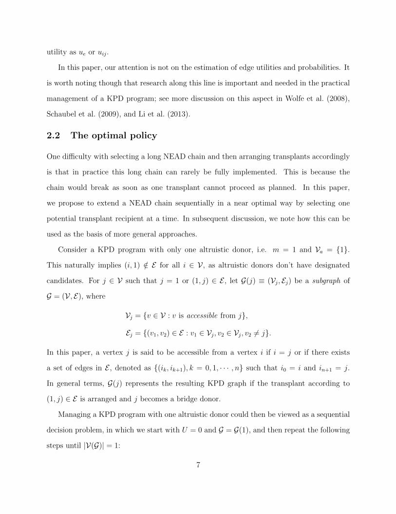
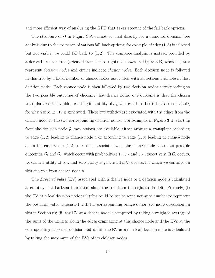
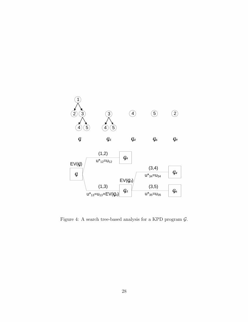
Figure 3-A provides an illustrative example, where G represents a KPD program with

four incompatible pairs (vertices 2, 3, 4 and 5) and one altruistic donor (vertex 1). Starting

from G, the action space is A = {(1, 2), (1, 3)} and suppose we proceed by selecting (1, 2).

If it is viable, this would lead to G(2), denoted as G9 in Figure 3-A, and the resulting value

of U∞ is u12; if (1, 2) is not viable, we end up with G1, at which the updated action space

becomes A = {(1, 3)}. We then continue by selecting (1, 3), and if it is not viable, we stop

at G2; if (1, 3) is viable, we then proceed to G3, at which the updated action space becomes

A = {(3, 4), (3, 5)}; and we continue this process by selecting one allocation from A. In this

paper, we assume that edges in a KPD graph have an independence relationship. Though

this assumption can be relaxed, it is a reasonable one when pair withdrawal (due to factors

such as pregnancy, illness, or death) does not occur frequently; see Li et al. (2013) for related

discussion.

[Figure 3 here]

3 Decision tree analysis for KPD

The optimal policy introduced in the previous section can be obtained by conducting a stan-

dard decision tree analysis, which we briefly illustrate below using a small example. The

computation associated with such an analysis, however, can be rather complicated for large

problems. We will return to this computational issue in Section 4, and present an alternative

and more efficient approach to analyzing policies and optimizing the allocations. Note that a

general mathematical framework derived from theories of Markov decision processes (MDPs)

can be used to rigorously formulate the problem of managing KPD programs with altruistic

donors (Li 2012). However, solving for the optimal policy is computationally difcult for large

or even moderate KPD problems, which poses a serious impediment to the development of

practical algorithms based on this MDP framework. We briefly describe the MDP formula-

tion in this section by using a particular example. In Section 4, we describe an alternative

9

and more efficient way of analyzing the KPD that takes account of the fall back options.

The structure of G in Figure 3-A cannot be used directly for a standard decision tree

analysis due to the existence of various fall-back options; for example, if edge (1, 3) is selected

but not viable, we could fall back to (1, 2). The complete analysis is instead provided by

a derived decision tree (oriented from left to right) as shown in Figure 3-B, where squares

represent decision nodes and circles indicate chance nodes. Each decision node is followed

in this tree by a fixed number of chance nodes associated with all actions available at that

decision node. Each chance node is then followed by two decision nodes corresponding to

the two possible outcomes of choosing that chance node: one outcome is that the chosen

transplant e ∈ E is viable, resulting in a utility of ue, whereas the other is that e is not viable,

for which zero utility is generated. These two utilities are associated with the edges from the

chance node to the two corresponding decision nodes. For example, in Figure 3-B, starting

from the decision node G, two actions are available, either arrange a transplant according

to edge (1, 2) leading to chance node a or according to edge (1, 3) leading to chance node

e. In the case where (1, 2) is chosen, associated with the chance node a are two possible

outcomes, G1 and G9, which occur with probabilities 1−p12 and p12 respectively. If G9 occurs,

we claim a utility of u12, and zero utility is generated if G1 occurs, for which we continue on

this analysis from chance node b.

The Expected value (EV) associated with a chance node or a decision node is calculated

alternately in a backward direction along the tree from the right to the left. Precisely, (i)

the EV at a leaf decision node is 0 (this could be set to some non-zero number to represent

the potential value associated with the corresponding bridge donor; see more discussion on

this in Section 6); (ii) the EV at a chance node is computed by taking a weighted average of

the sums of the utilities along the edges originating at this chance node and the EVs at the

corresponding successor decision nodes; (iii) the EV at a non-leaf decision node is calculated

by taking the maximum of the EVs of its children nodes.

10

For example, in Figure 3-B, the EVs at decision nodes G5 and G8 are EV [G5] = EV [d] =

p35u35 and EV [G8] = EV [h] = p34u34 respectively. The EVs at chance nodes c and g are

EV [c] = p34u34 + (1− p34)EV [G5] and EV [g] = p35u35 + (1− p35)EV [G8] respectively. This

indicates that EV [c] ≥ EV [g] if and only if u34 ≥ u35, and the action taken at G3 is therefore

(3, 4) or (3, 5) depending on which one has the larger edge utility. The EV at node G3 is

then calculated as

EV [G3] = max{EV [c], EV [g]}

= max{p34u34 + (1− p34)p35u35, p35u35 + (1− p35)p34u34}. (1)

After computing EVs associated with all decision and chance nodes in this way, the

optimal policy at each decision node is to adopt the action associated with the chance node

that has the maximum EV. This procedure starts from the root decision node, that is from

the altruistic donor.

4 A look-ahead search tree-based strategy

The structure of the derived decision tree in Figure 3-B is much more complicated than

the structure of G itself in Figure 3-A. As a result, the standard decision tree analysis as

introduced in Section 3 results in substantial computational difficulties when the KPD graph

is large. In this section, we address this issue by presenting a more efficient and practical

approach that relies on evaluating different allocations for each altruistic donor (or bridge

donor) according to a derived look-ahead search tree.

4.1 Identifying the optimal policy via a search tree

Consider first a KPD program, G = (V , E), where Va = {1},Vp = {2, 3, · · · , n}, and E =

{(1, i) : i = 2, 3, · · · , n}. Without loss of generality, assume u12 ≥ u13 ≥ · · · ≥ u1n. For this

specific KPD program, the optimal policy to follow at G is to try transplant (1, 2), and if it

11

fails then try (1, 3), then (1, 4) and so forth. The associated EV of this policy is

EV [G] =n∑

k=2

{u1kp1k

k−1∏i=2

(1− p1i)

}. (2)

Based on this fact, we could then select the optimal action to take from G directly and

hence avoid explicitly constructing a decision tree and calculating the EV associated with

each node of the tree, as would be required for the standard decision analysis in Section 3.

This observation is very useful as we can see, for example, by applying formula (2) at the

decision node G3 in Figure 3-B. This would lead to the optimal action of taking (3, 4) or

(3, 5) depending on which one has the larger utility; and the EV at G3 is therefore computed

as

EV [G3] = 1[u34≥u35] {p34u34 + (1− p34)p35u35}+ 1[u34<u35] {p35u35 + (1− p35)p34u34} . (3)

Note that formula (3) is exactly equal to the one calculated via a standard decision analysis

as in formula (1), but this latter approach requires calculating EVs at additional nodes G5

and G8.

Consider now a KPD program, G = (V , E), where Va = {1}, let A ≡ {(1, j) : (1, j) ∈ E}

and u∗1j ≡ u1j + EV [G(j)], for all (1, j) ∈ A. Without loss of generality, we assume A =

{(1, j) : j = 2, 3, · · · , l} and u∗12 ≥ u∗13 ≥ · · · ≥ u∗1l. Then the optimal decision to take at

G is to attempt transplant (1, 2); and if it fails, try (1, 3) and then (1, 4), and so on; the

associated EV is

EV [G] =l∑

k=2

{p1ku

∗1k

k−1∏i=2

(1− p1i)

}. (4)

Based on this result, we could evaluate various choices in A by u∗1j and then proceed with

the one having the largest value. We repeatedly apply this procedure from terminal nodes

up to sequentially form a NEAD chain, with formula (4) evaluating the expected utility in

this process.

12

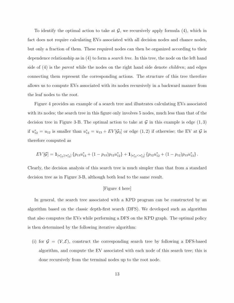
To identify the optimal action to take at G, we recursively apply formula (4), which in

fact does not require calculating EVs associated with all decision nodes and chance nodes,

but only a fraction of them. These required nodes can then be organized according to their

dependence relationship as in (4) to form a search tree. In this tree, the node on the left hand

side of (4) is the parent while the nodes on the right hand side denote children; and edges

connecting them represent the corresponding actions. The structure of this tree therefore

allows us to compute EVs associated with its nodes recursively in a backward manner from

the leaf nodes to the root.

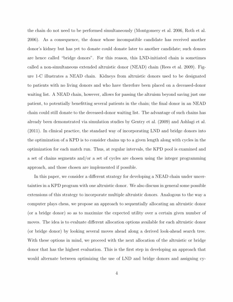
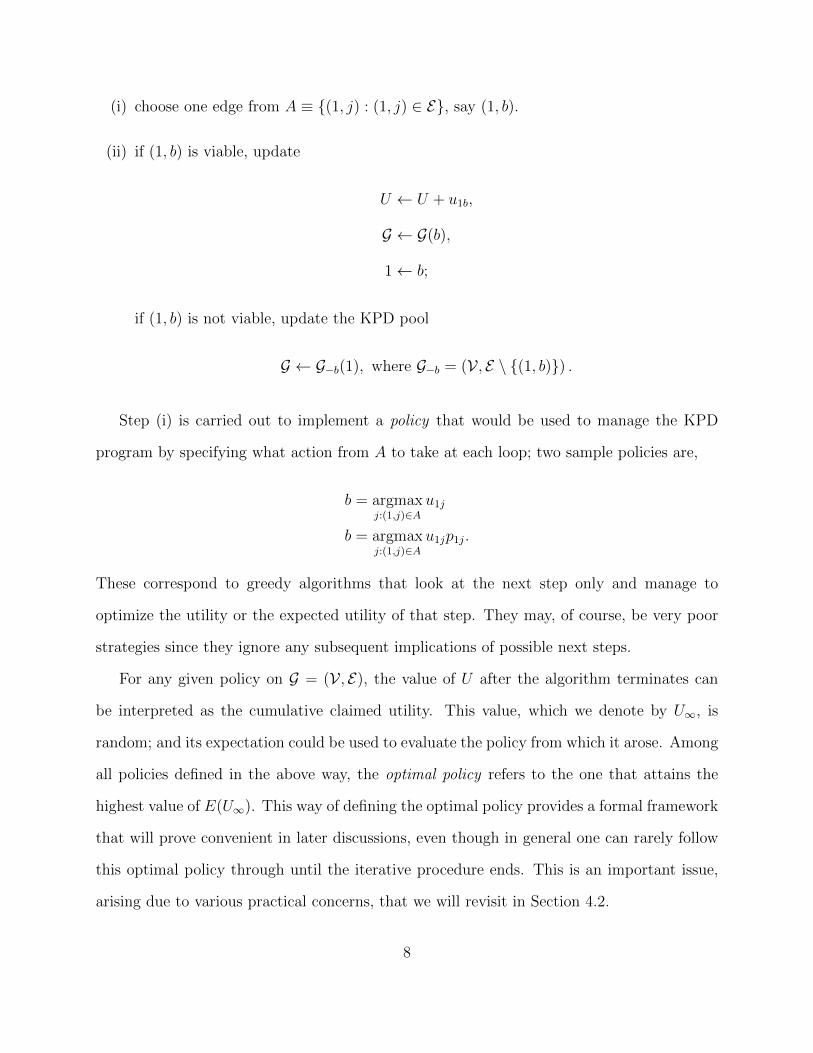
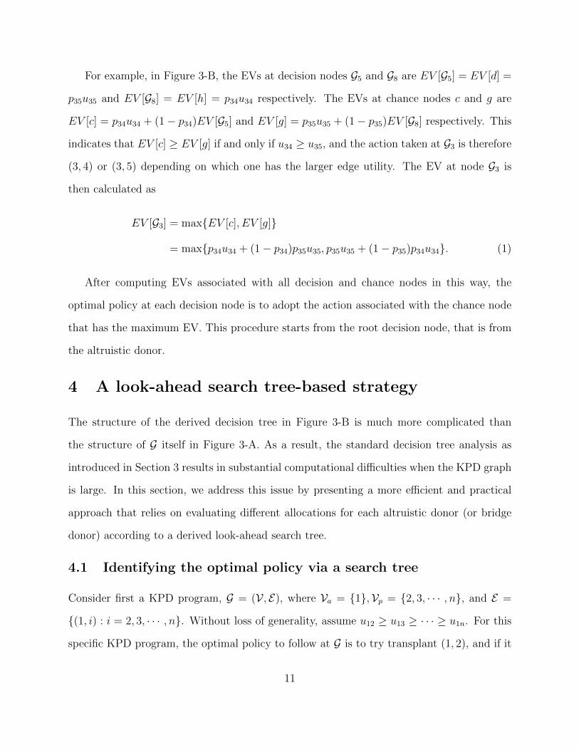
Figure 4 provides an example of a search tree and illustrates calculating EVs associated

with its nodes; the search tree in this figure only involves 5 nodes, much less than that of the

decision tree in Figure 3-B. The optimal action to take at G in this example is edge (1, 3)

if u∗12 = u12 is smaller than u∗13 = u13 + EV [G3] or edge (1, 2) if otherwise; the EV at G is

therefore computed as

EV [G] = 1[u∗13≥u∗

12]{p13u∗13 + (1− p13)p12u

∗12}+ 1[u∗

13<u∗12]{p12u∗12 + (1− p12)p13u

∗13} .

Clearly, the decision analysis of this search tree is much simpler than that from a standard

decision tree as in Figure 3-B, although both lead to the same result.

[Figure 4 here]

In general, the search tree associated with a KPD program can be constructed by an

algorithm based on the classic depth-first search (DFS). We developed such an algorithm

that also computes the EVs while performing a DFS on the KPD graph. The optimal policy

is then determined by the following iterative algorithm:

(i) for G = (V , E), construct the corresponding search tree by following a DFS-based

algorithm, and compute the EV associated with each node of this search tree; this is

done recursively from the terminal nodes up to the root node.

13

(ii) update the current action space A ≡ {(1, j) : (1, j) ∈ E(G)}, and calculate u∗1j =

u1j + EV [G(j)] for (1, j) ∈ A.

(iii) choose (1, b) ∈ A with b = argmaxj:(1,j)∈A u∗1j.

(iv) if (1, b) is viable, update

G ← G(b), i.e. update the KPD graph,

1← b, i.e. set the bridge donor b as the new altruistic donor;

if (1, b) is not viable, update the KPD pool

G ← G−b(1), where G−b = (V , E \ {(1, b)}) .

(v) go back to (ii) until |V(G)| = 1.

For completeness, we also briefly describe here a slightly more complicated example in

which the KPD itself is not a tree (as it is in Figure 3-A above). The KPD in this example is

obtained by adding edges (2, 4) and (4, 3) to the KPD graph G in Figure 3-A. Note that vertex

4 can be reached in two distinct ways and gives rise to two distinct subgraphs. Specifically, if

(1, 3) and (3, 4) are transplanted, G(4) only has vertex 4; if (1, 2) and (2, 4) are transplanted,

G(4) has vertices 4 and 3 and also contains edge (4, 3).

4.2 A depth-k search tree

Although the search tree-based approach allows for a much more efficient analysis than does

a standard decision tree analysis, constructing such a search tree is computationally very

expensive for a general large KPD graph; in fact, the computation is extensive even without

the effort entailed in computing EVs associated with nodes along that tree. This unfortunate

fact poses a substantial difficulty in identifying the optimal policy when the KPD program

is large.

14

Further, a more important issue is that the optimal policy (even if it could be computed)

would most likely not be implementable in practice. This is mainly because the practical

process of initiating and extending a NEAD chain would require a relatively long period of

time, during which the KPD pool would constantly be updated and evolve as new pairs arrive

and/or existing pairs withdraw or candidates die; in addition, candidates in the pool may

also be transplanted via exchanges among incompatible pairs or deceased donor kidneys from

the waiting list, since these would typically be arranged in parallel with the NEAD chain

mechanism. Thus, assessing strategies by looking a long way down the tree from the root

node is often not that useful in practice.

To address such problems, we propose to proceed by first deriving a subtree, which we call

a depth-k search tree, from the original search tree. Such a subtree can be readily obtained

by the same DFS-based algorithm as introduced in Section 4.1, by simply restricting the

depth of the search from the root node to k. We then follow the recursive relationship as

in formula (4) to calculate the EVs associated with corresponding nodes in the subtree,

beginning this calculation from the leaf nodes at depth k and working up through the tree to

the root node. The EV of a leaf node is set to zero or some reasonable measurement of the

value of the corresponding bridge donor (see Section 6 for more discussion). At this stage

the iterative procedure presented in Section 4.1 can be applied, but with one modification

that — if the chosen action (1, b) is viable, we regenerate a depth-k search tree rooted at

G(b) and compute EVs associated with the nodes of this new tree.

Instead of the optimality that exists only in a rather idealized scenario, the policy ob-

tained from the depth-k search tree provides a more practical evaluation of potential bridge

donors and a greatly reduced computational complexity. Further, our simulation results (see

Section 5) suggest that the allocation strategy derived from a search tree performs reasonably

well for a moderate depth of, say, 3 or 4. It is useful to note that this strategy is feasible in

the context of the search tree approach of this section, but would still be very complicated

15

to implement using the standard decision tree analysis; for example, the depth-1 search tree

constructed according to formula (2) provides the same analysis as the one via a standard

decision tree of depth 2n + 1.

5 Simulation studies

So far in this paper, we have explored a look-ahead search tree-based approach to manage a

KPD program with one altruistic donor. This approach sequentially extends a NEAD chain

by selecting one potential bridge donor at a time, taking into consideration the operational

uncertainties and the long-term consequences associated with various possible selections. In

this section, we provide simulation results of applying such an allocation strategy to manage

a simulated KPD program.

5.1 Simulating incompatible pairs and altruistic donors

We simulate incompatible pairs and altruistic donors as in Li et al. (2013). For an in-

compatible pair, we simulate its candidate and donor separately from their own population

distributions. Candidates are sampled at random (with replacement) from a database of

incompatible pairs, which is derived from the University of Michigan KPD program. This

database currently consists of 115 transplant candidates, each having at least one willing but

incompatible donor. We are in the process of incorporating additional databases from other

KPD programs for the purpose of reflecting a broader candidate variation. On the other

hand, donors are simulated by sampling their blood types and HLA haplotypes respectively.

Blood type is drawn from its U.S. population distribution: O, 44%; A, 42%; B, 10%; and

AB, 4% (Stanford Blood Center, 2010), and HLA haplotypes are sampled according to a

population frequency table derived from a public database on potential bone marrow donors

(Maiers et al. 2007).

We consider a simulated donor-candidate pair as an incompatible pair, and hence include

16

it in the KPD pool, if either their blood types mismatch or the donor’s HLA haplotypes

overlap with some of the candidate’s antibody specificities. Finally, an altruistic donor

is generated in the same way as we have described above for generating a donor in an

incompatible pair.

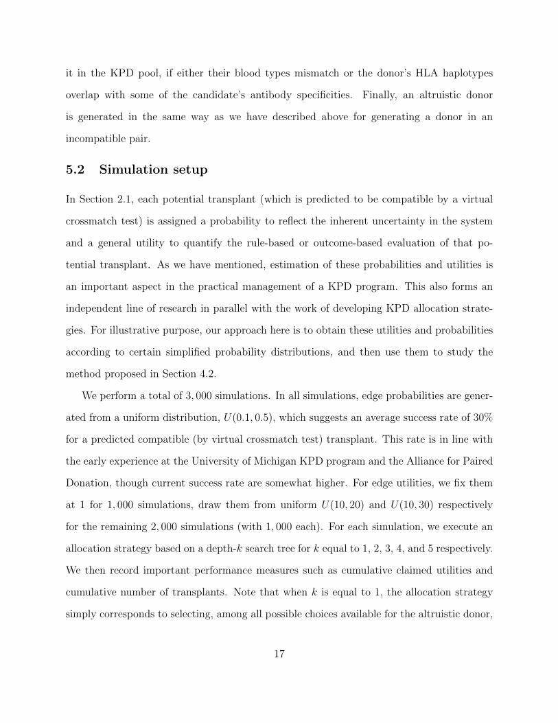
5.2 Simulation setup

In Section 2.1, each potential transplant (which is predicted to be compatible by a virtual

crossmatch test) is assigned a probability to reflect the inherent uncertainty in the system

and a general utility to quantify the rule-based or outcome-based evaluation of that po-

tential transplant. As we have mentioned, estimation of these probabilities and utilities is

an important aspect in the practical management of a KPD program. This also forms an

independent line of research in parallel with the work of developing KPD allocation strate-

gies. For illustrative purpose, our approach here is to obtain these utilities and probabilities

according to certain simplified probability distributions, and then use them to study the

method proposed in Section 4.2.

We perform a total of 3, 000 simulations. In all simulations, edge probabilities are gener-

ated from a uniform distribution, U(0.1, 0.5), which suggests an average success rate of 30%

for a predicted compatible (by virtual crossmatch test) transplant. This rate is in line with

the early experience at the University of Michigan KPD program and the Alliance for Paired

Donation, though current success rate are somewhat higher. For edge utilities, we fix them

at 1 for 1, 000 simulations, draw them from uniform U(10, 20) and U(10, 30) respectively

for the remaining 2, 000 simulations (with 1, 000 each). For each simulation, we execute an

allocation strategy based on a depth-k search tree for k equal to 1, 2, 3, 4, and 5 respectively.

We then record important performance measures such as cumulative claimed utilities and

cumulative number of transplants. Note that when k is equal to 1, the allocation strategy

simply corresponds to selecting, among all possible choices available for the altruistic donor,

17

the one that has the largest edge utility.

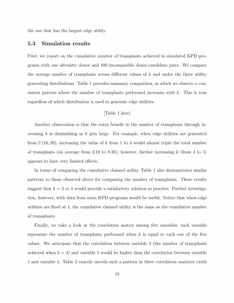
5.3 Simulation results

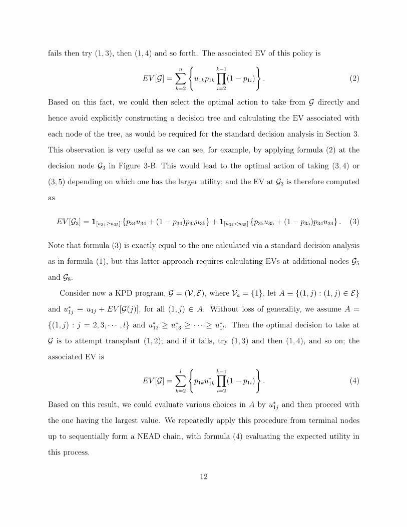
First, we report on the cumulative number of transplants achieved in simulated KPD pro-

grams with one altruistic donor and 100 incompatible donor-candidate pairs. We compare

the average number of transplants across different values of k and under the three utility

generating distributions. Table 1 provides summary comparison, in which we observe a con-

sistent pattern where the number of transplants performed increases with k. This is true

regardless of which distribution is used to generate edge utilities.

[Table 1 here]

Another observation is that the extra benefit in the number of transplants through in-

creasing k is diminishing as k gets large. For example, when edge utilities are generated

from U(10, 20), increasing the value of k from 1 to 4 would almost triple the total number

of transplants (on average from 3.18 to 8.26); however, further increasing k (from 4 to 5)

appears to have very limited effects.

In terms of comparing the cumulative claimed utility, Table 1 also demonstrates similar

patterns to those observed above for comparing the number of transplants. These results

suggest that k = 3 or 4 would provide a satisfactory solution in practice. Further investiga-

tion, however, with data from more KPD programs would be useful. Notice that when edge

utilities are fixed at 1, the cumulative claimed utility is the same as the cumulative number

of transplants.

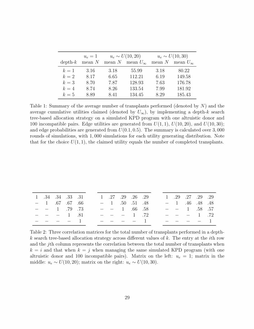
Finally, we take a look at the correlation matrix among five variables; each variable

represents the number of transplants performed when k is equal to each one of the five

values. We anticipate that the correlation between variable 4 (the number of transplants

achieved when k = 4) and variable 5 would be higher than the correlation between variable

1 and variable 5. Table 2 exactly unveils such a pattern in three correlation matrices (with

18

each one corresponding to one utility generating distribution). Similar observations are also

noted in the correlation matrices for the cumulative claimed utility.

[Table 2 here]

6 Concluding remarks

In this paper, we have studied the problem of managing a KPD program with one altruistic

donor. One important yet challenging part of this problem is to recognize various friction (as

discussed in Section 2.1) inherent in the system and to guide the decision-making process by

taking into account these uncertainties. Realizing the fact that a long pre-specified NEAD

chain in practice can almost never be implemented as planned, we propose to initiate and

extend such a chain in a sequential way by selecting potential transplant recipients one at

a time. Each selection is made keeping in mind the associated long-term consequences so

as to maximize the expected gain over a certain given number of moves. In order to do

this efficiently and practically, we construct a depth-k search tree for a KPD graph using a

DFS-based algorithm. We then evaluate various choices available for each altruistic donor (or

bridge donor) according to the calculation performed along that search tree, and recommend

the choice with the greatest expected utility.

In the process of extending a NEAD chain, the bridge donor at the end of the current

chain might be incompatible with a majority of the candidate population, which would

significantly prolong the waiting time for that bridge donor to be matched with a present or

future candidate. Furthermore, this long waiting time for the hard-to-match bridge donor

may make him/her more likely to withdraw from the KPD pool and so terminate the NEAD

chain. To partially avoid this unfortunate circumstance, some KPD programs have not

allowed a blood type AB donor to become a bridge donor. Actually, this issue can be partially

addressed in our proposed sequential allocation strategy, which incorporates the long-term

consequences associated with each pair choice, and would in general tend to avoid choices

19

that could lead to a hard-to-match bridge donor. As we have briefly mentioned in Section 3

and Section 4.2, one way to further address this issue is to assign each possible bridge donor

a reasonable base utility. This base utility represents the potential “contribution” from a

bridge donor; a hard-to-match bridge donor would be assigned a small base utility and an

easy-to-match one would be given a larger value.

Although this paper has focused on managing a KPD program with one altruistic donor,

the proposed approach can be generalized to incorporate multiple altruistic donors. One

way to achieve this is to construct a depth-k search tree for each altruistic donor and use

this tree to evaluate various allocations options available for that altruistic donor according

to the method in Section 4.2. Among all allocations possible for these altruistic donors, we

select a disjoint collection such that the overall expected utility can be maximized. More

specifically, let Va ≡ {1, 2, · · · ,m} be m altruistic donors in a general KPD program. We

denote by A ≡ ∪mi=1{(i, j) ∈ E} the possible allocations available for these m altruistic

donors. Each potential transplant, (i, j) ∈ A, can be evaluated by its expected utility, which

is calculated as u∗ij = uij + EV [G[i](j)], where G[i] ≡ G(i). We then select from A a disjoint

collection of edges (or transplants), in the sense that no two edges can share a common

vertex, so as to maximize the sum of expected utilities. For those selected transplants,

viable ones would result in actual operations and generate new bridge donors, and altruistic

donors and incompatible pairs involved in non-viable transplants are recycled back to the

KPD pool.

The above way of allocating multiple altruistic donors can be arranged in parallel with the

selection of exchange sets (or cycles) among incompatible pairs. Let Sr be the collection of

all exchange sets of size up to r among (n−m) incompatible pairs (Li et al. 2013). Typically,

in clinical KPD programs, one chooses r = 3, although larger exchanges could be considered

as well. For each S ∈ Sr, let EUS represent its expected utility and let YS be a decision

variable equal to 1 if S is selected and 0 if not; for each (i, j) ∈ A, Zij is another decision

20

variable whose value is 1 if (i, j) is chosen for a transplant and 0 otherwise; the expected

utility of this potential transplant (i, j) is given by u∗ij as discussed above. By adopting a

formulation that is similar to the one proposed in Li et al. (2013), we then manage such a

KPD program by solving the following IP problem:

max{YS},{Zij}

∑S∈Sr

YSEUS +∑

(i,j)∈A

Ziju∗ij

, (5)

subject to∑

S∈Sr(l)

YS +∑

(i,j)∈A(l)

Zij ≤ 1,∀l ∈ V , (6)

where, in (6), Sr(l) represents the exchange sets in Sr that contain l and A(l) similarly

denotes a subset of transplants in A that involve l. Various extensions of this approach

would be possible to allow fall back options for the exchanges and for the assignment of the

altruistic donors. Such approaches are discussed in Li et al. (2013). This approach, and

extensions of it, provide an alternative to the simultaneous selection of chains and cycles as

is traditionally done in the match runs of a KPD; see for example, Roth et al. (2006), Gentry

et al. (2009), and Ashlagi et al. (2011).

The mechanism of a NEAD chain allows the altruism from a single altruistic donor

to benefit a potentially large number of patients, but it does so exclusively for patients

recruiting a willing but incompatible living donor. This mechanism excludes patients without

a designated living donor and who are therefore placed on a deceased-donor waiting list.

Among those patients who would benefit from this NEAD chain, approximately 73% of

them are white; whereas those who would not benefit from this mechanism form a 52% non-

white population (Segev et al. 2008). On the other hand, not all altruistic (or bridge) donors

are well suited for initiating and extending chains among a pool of incompatible pairs. For

example, consider a KPD pool in which an altruistic donor may not be in a good position

(because of either incompatibility or poor utility) to be matched up with any candidate.

In this case, rather than placing this altruistic donor in a waiting “mode” for a potentially

long time, redirecting him/her to a deceased-donor waiting list, where a compatible patient

21

with potentially good transplant outcomes might be identified rather easily, appears a more

suitable alternative.

To decide whether an altruistic donor is better off initiating a NEAD chain or donating

directly to someone on a deceased-donor waiting list, we could evaluate an altruistic donor by

the utility expected to be achieved if this donor is chosen to initiate a chain. To be precise,

we may first perform the calculation according to formula (4) as in Section 4.1 to evaluate

the expected utility for each altruistic donor, i.e. {EV [G(i)] : i ∈ Va}. The result from this

evaluation could then be used to assess the suitability of assigning each altruistic donor to a

deceased-donor waiting list; a relatively high value of EV [G(i)] would recommend reserving

altruistic donor i for extending a NEAD chain while a comparatively low value of EV [G(i)]

would indicate a transplant to someone waiting for a deceased-donor kidney. It is worth

noting that different ways of assigning edge utilities and probabilities could be adopted in

calculating {EV [G(i)] : i ∈ Va}. This would provide extra benefit in allowing more control

over what kidneys in general are distributed to a deceased-donor waiting list. For example,

if each edge is assigned an equal utility while the edge probability remains representing the

likelihood of that edge being viable, then altruistic (or bridge) donors who are less compatible

with candidates in the current KPD pool would be more likely to be directed to a deceased-

donor waiting list. In addition to evaluating an altruistic donor against the current KPD

pool, it is often rational in practice to perform the evaluation against the deceased-donor

waiting list. For example, Blood Type O or B candidates frequently wait a year or more

longer on the deceased-donor waiting list before receiving a kidney transplant than do Blood

Type A or AB candidates. Therefore a Blood Type O or B altruistic or bridge donor might

be argued to have higher utility. So might someone who matches to a pediatric candidate.

Similarly an altruistic or bridge donor that might match to a sensitized wait-listed candidate

might have a higher utility, but a lower probability of progressing to transplant.

22

Acknowledgements

This work was supported in part by a grant from the National Institutes of Health (NIH)

CTSA at the University of Michigan 2UL1TR000433-06 and by the NIH grant 1R01-DK093513.

The authors thank the support from the Michigan Institute for Clinical and Health Research

(MICHR), Michigan School of Public Health, Scientific Registry of Transplant Recipients,

and National Institute of General Medical Sciences (NIGMS). Last but not least, the au-

thors would like to thank the editor and referees whose comments helped to improve this

manuscript.

References

Abraham, D. J., Blum, A., and Sandholm, T. (2007). Clearing algorithms for barter exchange

markets: Enabling nationwide kidney exchanges. Ec’07: Proceedings of the Eighth Annual

Conference on Electronic Commerce, pages 295–304.

Ashlagi, I., Gilchrist, D. S., Roth, A. E., and Rees, M. A. (2011). Nonsimultaneous chains

and dominos in kidney-paired donation - revisited. American Journal of Transplantation,

11(5):984–994.

Evans, R. W., Manninen, D. L., Garrison, L. P., Hart, L. G., Blagg, C. R., Gutman, R. A.,

Hull, A. R., and Lowrie, E. G. (1985). The quality of life of patients with end-stage renal

disease. New England Journal of Medicine, 312(9):553–559.

Gentry, S. E., Montgomery, R. A., Swihart, B. J., and Segev, D. L. (2009). The roles of

dominos and nonsimultaneous chains in kidney paired donation. American Journal of

Transplantation, 9(6):1330–1336.

Li, Y. (2012). Optimization and simulation of kidney paired donation programs (doctoral

dissertation). University of Michigan, Ann Arbor.

23

Li, Y., Kalbfleisch, J. D., Song, P. X.-K., Zhou, Y., Leichtman, A. B., and Rees, M. A. (2013).

Optimal decisions for organ exchanges in a kidney paired donation program. Statistics in

Biosciences.

Maiers, M., Gragert, L., and Klitz, W. (2007). High-resolution hla alleles and haplotypes in

the united states population. Human Immunology, 68(9):779–788.

Montgomery, R. A., Gentry, S. E., Marks, W. H., Warren, D. S., Hiller, J., Houp, J., Zachary,

A. A., Melancon, J. K., Maley, W. R., Rabb, H., Simpkins, C., and Segev, D. L. (2006).

Domino paired kidney donation: a strategy to make best use of live non-directed donation.

The Lancet, 368(9533):419–421.

Rapaport, F. T. (1986). The case for a living emotionally related international kidney donor

exchange registry. Transplantation Proceedings, 18:5–9.

Rees, M. A., Kopke, J. E., Pelletier, R. P., Segev, D. L., Rutter, M. E., Fabrega, A. J.,

Rogers, J., Pankewycz, O. G., Hiller, J., Roth, A. E., Sandholm, T., Unver, M. U., and

Montgomery, R. A. (2009). A nonsimultaneous, extended, altruistic-donor chain. New

England Journal of Medicine, 360(11):1096–1101.

Roth, A. E., Sonmez, T., and Unver, M. U. (2004). Kidney exchange. Quarterly Journal of

Economics, 119(2):457–488.

Roth, A. E., Sonmez, T., and Unver, M. U. (2007). Efficient kidney exchange: Coincidence

of wants in markets with compatibility-based preferences. American Economic Review,

97(3):828–851.

Roth, A. E., Sonmez, T., Unver, M. U., Delmonico, F. L., and Saidman, S. L. (2006).

Utilizing list exchange and nondirected donation through ‘chain’ paired kidney donations.

American Journal of Transplantation, 6(11):2694–2705.

24

Russell, J. D., Beecroft, M. L., Ludwin, D., and Churchill, D. N. (1992). The quality of life

in renal transplantation-a prospective study. Transplantation, 54(4):656–660.

Schaubel, D. E., Wolfe, R. A., Sima, C. S., and Merion, R. M. (2009). Estimating the

effect of a time-dependent treatment by levels of an internal time-dependent covariate:

Application to the contrast between liver wait-list and posttransplant mortality. Journal

of the American Statistical Association, 104(485):49–59.

Segev, D. L., Kucirka, L. M., Gentry, S. E., and Montgomery, R. A. (2008). Utilization and

outcomes of kidney paired donation in the united states. Transplantation, 86(4):502–510.

Wolfe, R. A., Ashby, V. B., Milford, E. L., Ojo, A. O., Ettenger, R. E., Agodoa, L. Y. C.,

Held, P. J., and Port, F. K. (1999). Comparison of mortality in all patients on dialysis,

patients on dialysis awaiting transplantation, and recipients of a first cadaveric transplant.

New England Journal of Medicine, 341(23):1725–1730.

Wolfe, R. A., McCullough, K. P., Schaubel, D. E., Kalbfleisch, J. D., Murray, S., Stegall,

M. D., and Leichtman, A. B. (2008). Calculating life years from transplant (lyft): Meth-

ods for kidney and kidney-pancreas candidates. American Journal of Transplantation,

8(4p2):997–1011.

25

donor 1 candidate 1

donor 2 candidate 2

donor 1 candidate 1

donor 2 candidate 2

altruistic donor 1

donor 2 candidate 2

donor 3 candidate 3 donor 3 bridge donor candidate 3

(A) (B) (C)

Figure 1: (A): A two-way exchange; (B): A three-way exchange; (C): A NEAD chain.

1 2

3

1 2

1 2

3

(A) (B) (C)

Figure 2: (A): A graph representation of a KPD program with a two-way exchange cycle,where Vp = {1, 2} and E = {(1, 2), (2, 1)}; (B): A graph representation of a KPD programwith a three-way exchange cycle, where Vp = {1, 2, 3} and E = {(1, 2), (2, 3), (3, 1)}; (C): Agraph representation of a NEAD chain, where Va = {1}, Vp = {2, 3} and E = {(1, 2), (2, 3)};donor 3 at the end of the chain becomes a bridge donor.

26

G

a

e

G9

G1 b

G2

G3

G10 f

G2

G9

(1,2)G3

c

G5

G4

g

G8

G6

d

G7

G6

h

G7

G4

p12

1-p12(1,3)

1-p13

p13

(3,4)

(3,5)

p34

p35

1-p34 (3,5)

p35

1-p35

1-p35 (3,4)

p34

1-p34

(1,3)

1-p13 (1,2)

p12

1-p12

p13

2

1

3

54

1

3

54

1 3

54

4 3

5

5 3 3

4

2 1

2

G G1 G2 G3 G4 G5 G6 G7 G8 G9 G10

(A)

(B)

u12

u13

u34

u35

u34

u35

u13

u12

0

0

0

0

0

0

0

0

Figure 3: (A): A KPD program G with one altruistic donor and four incompatible pairs aswell as various subgraphs of G; (B): A standard decision tree analysis for a KPD program Gas in (A), with squares representing decision nodes and circles indicating chance nodes; thedecision node G3 (which is shaded) appears twice in the tree and hence is only drawn once.

27

G

(1,2)

(1,3)

2

1

3

54

3

54

4 5 2

G G3 G4 G6 G9

G9

G3 G6

G4

(3,4)

(3,5)

u*34=u34

u*35=u35

EV(G3)

u*12=u12

u*13=u13+EV(G3)

EV(G)

Figure 4: A search tree-based analysis for a KPD program G.

28

ue = 1 ue ∼ U(10, 20) ue ∼ U(10, 30)depth-k mean N mean N mean U∞ mean N mean U∞

k = 1 3.16 3.18 55.99 3.18 80.22k = 2 8.17 6.65 112.21 6.19 149.58k = 3 8.70 7.87 128.93 7.63 176.78k = 4 8.74 8.26 133.54 7.99 181.92k = 5 8.89 8.41 134.45 8.29 185.43

Table 1: Summary of the average number of transplants performed (denoted by N) and theaverage cumulative utilities claimed (denoted by U∞), by implementing a depth-k searchtree-based allocation strategy on a simulated KPD program with one altruistic donor and100 incompatible pairs. Edge utilities are generated from U(1, 1), U(10, 20), and U(10, 30);and edge probabilities are generated from U(0.1, 0.5). The summary is calculated over 3, 000rounds of simulations, with 1, 000 simulations for each utility generating distribution. Notethat for the choice U(1, 1), the claimed utility equals the number of completed transplants.

1 .34 .34 .33 .31− 1 .67 .67 .66− − 1 .79 .73− − − 1 .81− − − − 1

1 .27 .29 .26 .29− 1 .50 .51 .48− − 1 .66 .58− − − 1 .72− − − − 1

1 .29 .27 .29 .29− 1 .46 .48 .48− − 1 .58 .57− − − 1 .72− − − − 1

Table 2: Three correlation matrices for the total number of transplants performed in a depth-k search tree-based allocation strategy across different values of k. The entry at the ith rowand the jth column represents the correlation between the total number of transplants whenk = i and that when k = j when managing the same simulated KPD program (with onealtruistic donor and 100 incompatible pairs). Matrix on the left: ue = 1; matrix in themiddle: ue ∼ U(10, 20); matrix on the right: ue ∼ U(10, 30).

29