decision support tools for ... - university of toronto
TRANSCRIPT

Decision Support Tools for Sustainable Water Distribution Systems
by
Rebecca M. Dziedzic
A report submitted in conformity with the requirements for the degree of Doctor of Philosophy
Graduate Department of Civil Engineering University of Toronto
© Copyright by Rebecca M. Dziedzic 2015

ii
Decision Support Tools for Sustainable Water Distribution
Systems
Rebecca M. Dziedzic
PhD Candidate
Graduate Department of Civil Engineering University of Toronto
2015
Abstract
Sustainability relies on the balance between economic, social, and environmental objectives.
Although seemingly divergent at times, the connections between them elucidate opportunities for
improving different components simultaneously. In water distribution systems, aging
infrastructure, insufficient funds, water scarcity, leakage, and high energy use have prompted the
pursuit of sustainability through different strategies. These conditions demand improvement and
create the opportunity to rethink the system. The present study proposes five separate decision
support approaches that underlie a systems approach. These address current issues of North
American water distribution systems and lessen the gap between research and application.
The first two focus on the interface between users and networks. The relation between user
characteristics and demand is studied by building an integrated database to support planning,
especially demand management. Data from three Ontario municipalities are used to define
metrics, benchmarks, conservation targets, and user clusters. The relation between users and
service requirements is further explored qualitatively through a survey on water user
expectations, addressing the disconnection between utilities and stakeholders. Applied to the City
of Guelph, it informs the utility of knowledge gaps and preferred solutions.

iii
While these approaches concentrate on the needs of the stakeholders, inputs to more thorough
planning, the next two assess the resulting systems. A set of energy metrics addresses the issue of
inefficient energy use and provides indicators of system capacity, costs, and greenhouse gas
emissions. The metrics are applied to the Toronto water network, and allow for the identification
of specific areas for improvement. In order to further evaluate how complex networks respond to
variations, a more comprehensive set of performance metrics are proposed and applied to two
example networks.
The final approach seeks to improve the design process by reducing the computational intensity
of optimization procedures and thereby allowing for the analysis of more system objectives and
uncertainties. The procedure, applied to Anytown, uses shorter time cycles to approximate full
costs of systems with varying loads. Overall, the approaches facilitate current-day decision-
making by applying systems thinking to the development of new solutions that collect, integrate,
analyse, and re-interpret readily available data and models.

iv
Acknowledgments
There are a number of people, institutions, and municipal water utilities that supported my
doctoral research. The first of these that I would like to thank is the person who took a leap of
faith and opened University of Toronto’s metaphorical door to me. Professor Bryan W. Karney
consistently found new research projects and potential collaborations, which allowed me to apply
my research to real water distribution systems. His supervision motivated me to analyse water
systems without preconceptions, and question current paradigms. Furthermore, his careful
revision of multiple versions of the studies presented herein greatly improved how they are
articulated in the thesis. Thank you for your always encouraging words.
Throughout the writing of the thesis I also received invaluable constructive criticism from
professors in different fields, which significantly strengthened the work and contributed to its
multidisciplinary nature. I thank my supervisory committee and external reviewer for selflessly
taking the time to scrutinize the thesis. Specifically, I thank Professor Tamer El-Diraby for
continuously emphasizing the need to clearly state the value of the work. Thanks are also
extended to Professor Jennifer Drake for meticulously reviewing the thesis document and
questioning unclear arguments. Additionally, I thank Professor Bryan Tolson, of the University
of Waterloo, for his truly insightful comments, which helped enhance the thesis and more
explicitly demonstrate the improvement achieved by applying the proposed tools. Moreover,
many thanks are extended to Professor Ingrid L. Stefanovic, who even after becoming Dean of
the Faculty of Environment at Simon Fraser University, travelled back to Toronto twice, to
participate in the departmental and final defenses. Her guidance, especially regarding the social
implications of decisions, was invaluable to the production of the thesis and to my development
as a researcher.
The thesis not only contains three studies that were applied to Ontario water utilities but was
largely shaped by these interactions, which elucidated the needs of current local water systems
and the gaps between research and practice. Two of these projects were made possible through
the Showcasing Water Innovation program funded by the Ontario Ministry of the Environment.
As part of these projects, I had the privilege to work with Kathryn Grond from the University of
Toronto’s Cities Centre, as well as Katelyn Margerm and Tom Weatherburn from the Canadian
Urban Institute, and to be supervised by Jeff Evenson. These people guided me through the

v
essentials of practical research. I also thank the water service divisions of the cities of Barrie,
Guelph, London, and Toronto, for believing in the potential of the research, supporting the
studies, sharing information, and discussing the applications of the work. Specific thanks are
extended to the managers in each municipal utility, who coordinated internal efforts: Barry
Thompson, Wayne Galliher, Matt Feldberg, and Abhay Tadwalkar, respectively.
Finally, I must thank my family for unconditionally supporting this dream, even if it meant being
more than 9,000 km away. I thank my mother for giving me solace, crying with me during the
challenging times, and continuously trying to cheer me up. I also thank my sister for her
companionship and ability to keep me grounded. Lastly, I dedicate this thesis to my eternal
supervisor and mentor, my father. Thank you for the numerous revisions and late night
discussions of the research.

vi
Table of Contents
Acknowledgments.................................................................................................................................iv!
Table.of.Contents...................................................................................................................................vi!
List.of.Tables...........................................................................................................................................ix!
List.of.Figures.........................................................................................................................................xi!
1! Introduction......................................................................................................................................1!1.1! Re?envisioning.our.Water.Systems..................................................................................................1!1.2! Thesis.Objectives...................................................................................................................................4!1.3! Overview.and.Layout............................................................................................................................6!1.4! Publications.Related.to.Thesis.Research.......................................................................................9!
2! Sustainability.of.Water.Distribution.Systems.....................................................................12!2.1! Definitions.of.Sustainability.............................................................................................................12!2.2! Water.Distribution.System.Assessment.......................................................................................13!2.3! Conceptual.Map.of.the.System.........................................................................................................18!
3! Integrated.Database.for.Demand.Management..................................................................28!3.1! The.Value.of.Integrating.Data..........................................................................................................28!3.2! Methodology..........................................................................................................................................32!3.2.1! Problem!Definition!.......................................................................................................................................!32!3.2.2! Data!Preparation!...........................................................................................................................................!33!3.2.3! Data!Exploration!...........................................................................................................................................!36!3.2.4! Modeling!...........................................................................................................................................................!37!3.2.5! Evaluation!........................................................................................................................................................!41!3.2.6! Deployment!.....................................................................................................................................................!41!
3.3! Results.....................................................................................................................................................41!3.4! Discussion..............................................................................................................................................48!3.5! Conclusions............................................................................................................................................50!
4! Collectively.Re?envisioning.the.Water.Utility.Business.Model......................................52!4.1! The.Water.Utility.Business.Model.and.the.Role.of.Stakeholder.Feedback......................53!4.2! User.Expectations.of.Service.in.Guelph........................................................................................57!4.2.1! Objectives!.........................................................................................................................................................!57!
vii
4.2.2! Methodology!...................................................................................................................................................!57!4.2.3! Results!...............................................................................................................................................................!58!4.2.4! Discussion!and!Business!Connections!.................................................................................................!64!
4.3! Conclusion..............................................................................................................................................71!
5! Energy.Metrics................................................................................................................................74!5.1! Introduction...........................................................................................................................................74!5.2! Methodology..........................................................................................................................................77!5.2.1! Metrics!...............................................................................................................................................................!77!5.2.2! Potential!Applications!of!the!Proposed!Energy!Metrics!..............................................................!81!
5.3! Case.Study.of.the.Toronto.Water.Distribution.System...........................................................83!5.3.1! Results!and!Discussion!...............................................................................................................................!85!
5.4! Conclusions............................................................................................................................................95!
6! Performance.Metrics....................................................................................................................97!6.1! Performance.of.water.distribution.networks.and.other.complex.systems.....................97!6.2! Performance.Index...........................................................................................................................102!6.3! Case.Studies........................................................................................................................................106!6.3.1! Example!Network!1!...................................................................................................................................!108!6.3.2! Example!Network!2!...................................................................................................................................!112!
6.4! Critical.Appraisal..............................................................................................................................122!6.5! Conclusions.........................................................................................................................................123!
7! Cost.Gradient.Search.Optimization.Technique................................................................124!7.1! Introduction........................................................................................................................................124!7.2! A.Brief.Literature.Review.of.Optimization.Techniques.......................................................126!7.3! Methodology.......................................................................................................................................131!7.4! Anytown.Case.Study.........................................................................................................................135!7.5! Results.and.Discussion...................................................................................................................137!7.6! Initial.Assessment.of.the.Proposed.Methodology..................................................................140!7.7! Conclusions.........................................................................................................................................142!
8! Conclusions.and.Future.Steps................................................................................................143!8.1! Summary.of.Contributions.and.Conclusions...........................................................................143!8.2! Future.Research................................................................................................................................147!
References...........................................................................................................................................150!

viii
Appendix.A! Guelph.Water.User.Survey.–.Expectations.of.Service................................162!A.1! Collection.Notice...............................................................................................................................162!A.2! Water.User.Survey............................................................................................................................163!

ix
List of Tables
Table 4.1: Comparison of respondent and Guelph resident demographics. ................................. 59!
Table 4.2: Respondent awareness and performance rating of water system components. ........... 59!
Table 6.1: Elevation and demand values for Network 1 nodes. ................................................. 109!
Figure 6.2: Schematic representation of Network 1with node IDs. Table 6.2: Length, diameter,
and roughness coefficient values for Network 1 pipes. .............................................................. 109!
Table 6.3: Average energy metrics of the alternative configurations of Network 1, L – fewer
loops, D – larger diameters. ........................................................................................................ 110!
Table 6.4: Proposed performance metrics, resilience index (Todini, 2000), network resilience
index (Prasad and Park, 2004), modified resilience index (Jayaram and Srinivasam, 2008), and
average pressure of the alternative configurations of Network 1, L – fewer loops, D – larger
diameters. .................................................................................................................................... 112!
Table 6.5: Pump curve coordinates, flow and head, for Network 2. .......................................... 113!
Table 6.6: Tank levels for Network 2. ........................................................................................ 113!
Table 6.7: Elevation and demand values for Network 2 nodes. ................................................. 115!
Table 6.8: Length, diameter, and roughness coefficient values for Network 2 pipes. ................ 116!
Table 6.9: Average energy metrics of the alternative configurations of Network 2, L – fewer
loops, D – larger diameters, S – reduced storage, P – reduced pumping. ................................... 118!
Table 6.10: Proposed performance metrics, resilience index (Todini, 2000), network resilience
index (Prasad and Park, 2004), modified resilience index (Jayaram and Srinivasam, 2008), and
average pressure of the alternative configurations of Network 2, L – fewer loops, D – larger
diameters, S – reduced storage, P – reduced pumping. .............................................................. 120!
Table 7.1: Damage function for Anytown example based on Filion et al. (2007). .................... 133!

x
Table 7.2: Pipe sizes and expected costs for Anytown design solutions: (I) original problem, (II)
10% decreased demand growth, and (III) doubled damage costs. .............................................. 138!

xi
List of Figures
Figure 2.1: Causal loop diagrams for an urban water resource system: (a) water use and
conservation; (b) land-use/population; (c) land-use/hydrologic cycle (Giacomini et al., 2013). . 18!
Figure 2.2: Feedback loops involving finances of water distribution systems (Rehan et al., 2013).
....................................................................................................................................................... 19!
Figure 2.3: Feedback loops involving customer behavior in water distribution systems (Rehan et
al., 2013). ...................................................................................................................................... 19!
Figure 2.4: Feedback loops involving physical conditions of water distribution systems (Rehan et
al., 2013). ...................................................................................................................................... 20!
Figure 2.5: Causative factors and feedback loops of water distribution systems (Colombo and
Karney, 2003). .............................................................................................................................. 21!
Figure 2.6: Conceptual map of a water distribution system. ........................................................ 23!
Figure 3.1: Geographic levels of the different data types and their spatial relations. ................... 35!
Figure 3.2: Percentage of water use and users per segment: (a) total water consumption per
sector; (b) residential water consumption per property code; (c) residential water users per
consumption range in liters per capita per day; (d) commercial water consumption per property
code; (e) industrial water consumption per property code; (f) institutional water consumption per
property code. ............................................................................................................................... 42!
Figure 3.3: Yearly and seasonal residential water consumption trends from 2006 to 2011: (a)
total use in London; (b) total use in Barrie; (c) total use in Guelph; and in all three cities (d) use
per capita; (e) use per hectare; and (f) use per unit. ...................................................................... 43!
Figure 3.4: Residential water consumption per capita by building vintage for Barrie, Guelph, and
London. ......................................................................................................................................... 45!
Figure 3.5: Percentage of total water use and coefficient of variation of water use metrics for the
largest water using property codes in Barrie, ON, Canada. .......................................................... 46!

xii
Figure 4.1: Most important issues presently facing Guelph’s water system according to
respondents ................................................................................................................................... 61!
Figure 4.2: Motivations for respondents to conserve water. ......................................................... 62!
Figure 5.1: Schematic representation of the different forms of energy in a water distribution
system with a single reservoir, pump, pipe and tank. ................................................................... 78!
Figure 5.2: Skeletonized Toronto water distribution network. ..................................................... 84!
Figure 5.3: Partition of energy supplied between potential, delivery, and dissipation during the
summer (a) and winter (b) scenarios. ............................................................................................ 86!
Figure 5.4: Total energy dissipated per hour by pipes, pumps, and valves, during the summer (a)
and winter (b) scenarios. ............................................................................................................... 86!
Figure 5.5: Total energy delivered per hour to tanks and junctions, during the summer (a) and
winter (b) scenarios. ...................................................................................................................... 87!
Figure 5.6: Average head (pressure and kinetic) and total demand at junctions per hour, during
the summer (a) and winter (b) scenarios. ...................................................................................... 88!
Figure 5.7: Energy supplied by tanks and GHG emission factor per hour, during the summer (a)
and winter (b) scenarios. ............................................................................................................... 89!
Figure 5.8: Energy supplied by pumps, and water rate per hour, during the summer (a) and winter
(b) scenarios. ................................................................................................................................. 89!
Figure 5.9: Demand delivered to junctions and energy delivered to tanks per hour, during the
summer (a) and winter (b) scenarios. ............................................................................................ 90!
Figure 5.10: Energy supplied by pumps (a) and delivered to junctions (b) during the summer
scenario for the original and modified pump controls. ................................................................. 91!
Figure 5.11: Map of energy dissipated in the Toronto water distribution network during peak
demand (8 p.m.) on maximum demand day. ................................................................................ 92!

xiii
Figure 5.12: Map of energy supplied in the Toronto water distribution network during peak
demand (8 p.m.) on maximum demand day. ................................................................................ 93!
Figure 5.13: Map of energy delivered in the Toronto water distribution network during peak
demand (8 p.m.) on maximum demand day. ................................................................................ 93!
Figure 6.1: Peaking coefficients for Networks 1 and 2. ............................................................. 107!
Figure 6.2: Schematic representation of Network 1with node IDs. Table 6.2: Length, diameter,
and roughness coefficient values for Network 1 pipes. .............................................................. 109!
Figure 6.3: Energy efficiency profile over 24-hour simulation for Network 1 (a) original network,
(b) fewer loops, (c) larger diameters. .......................................................................................... 111!
Figure 6.4: Schematic representation of Network 2 with node IDs. ........................................... 114!
Figure 6.5: Energy efficiency profile over 24-hour simulation for Network 2 (a) original network,
(b) reduced storage, (c) reduced storage and pumping. .............................................................. 119!
Figure 7.1 : Algorithm for iterative dynamic optimization of water distribution networks. ...... 132!
Figure 7.2: Anytown network of Walski et al. (1987) with additional tank proposed by Gessler
(1985). ......................................................................................................................................... 136!

1
1 Introduction
1.1 Re-envisioning our Water Systems
Historically, water infrastructure was widely developed and installed throughout the 20th century.
As a result of both this long history and a certain complacency that developed with the newly
constructed systems, many systems face the current challenge of managing aging mains,
appurtenances, and equipment, more subject to leakage, failure, and in need of costly
replacement. Certainly experience has been gained, technologies have advanced, and in the era
of information, with better and less expensive sensors, computing, and communication, more
data can now be collected and processed than ever before. Given this convenience, the task of
nearly replacing entire systems can be seen as an opportunity to right the wrongs, to adjust
design to the new paradigm of sustainability. Much of the data collected, however, is not used to
its full potential, an issue addressed in chapter 3.
Designing, operating, and maintaining water supply systems is generally perceived as an
engineering problem. The goal is to deliver clean water to users according to standards that
ensure safe and adequate service. Within the ranges allowed by these standards, design and
operation is then adjusted to meet consumer requirements and theoretically minimize (or at least
constrain) costs. This obviously depends on the definition of costs, the possible inclusion of
various externalities, and the time span considered in decision making. These issues are further
explored in chapters 6 and 7, in which a performance index, and a cost-based optimization
technique are proposed, respectively. If the quality of the service produced by the system
depends so much on what has been defined as safe, reliable, and satisfactory, then one question
begs to be answered. Have we defined performance appropriately, that is, are the objectives and
constraints of this “problem” correctly stated?
Nevertheless, it is only fair to admit that even this query is instilled with an engineering bias.
From a physical perspective, the problem to be solved by water distribution is to move a liquid
with given properties from a source to the various locations of demand. In order to do so, a set of

2
pipes and appurtenances is designed and built. As the liquid passes through these components not
only may there be leaks, but mechanical energy is irreversibly converted to thermal energy,
becoming both less valuable and less available for other uses. From a strictly physical standpoint,
an efficient system should tightly limit the amount of water lost, energy wasted, and materials
used.
A water supply system, however, is more than a collection of engineered pieces – it is intended
to supply a need that is highly human. And because humans are complex, water demands are
hard to predict, particularly considering they fluctuate moment by moment, as well as hourly,
seasonally, yearly. Historical data can be used to predict future demands as well as support
conservation strategies, an application explored in chapter 3. Demand greatly depends on
customer behaviour as well as their response to pricing, technological and conservation
initiatives. Water supply systems physically connect the natural source of water to the
consumers, which may be residential, commercial, industrial, or agricultural, located, perhaps in
a seemingly haphazard manner. The gamut of services delivered includes hydration, sanitation,
cooling, increasing human comfort, aesthetic enhancement, facilitating or limiting the rate of
chemical reactions, and firefighting. These, among other regional, cultural, and climatological
differences lead consumers to use and perceive water differently. Feedback from the users, as
sought in chapter 4, can help utilities understand these distinctions as well as identify system
issues.
The availability of water can also vary. Changes in the balance of the water cycle due to global
warming might increase or decrease local water availability and will almost certainly alter
demand. The mitigation of these impacts would require the reduction of greenhouse gas
emissions. Adaptation might also include the alteration of operations and infrastructure. In
chapter 5, greenhouse gas emissions due to energy use are calculated and their variation
according to demands and time of day are discussed.
Still, from another perspective, economic, the goal of the utility is to deliver water to the
consumer while producing controlled or perhaps even minimum expenditures and receiving

3
sufficient revenue to cover capital and operational costs, as well as externalities. Water system
decision-making is multi-objective; it is bound by policies, and legislation, yet engulfed in
environmental, social, and economic considerations and goals. The balance of these three, it is
argued here, is the goal of sustainability, hence they cannot be analysed separately nor their
interactions discarded. However, an excessive number of factors can hinder the planning process.
Models, for instance, become too complex and computationally intensive. A map that is too
detailed can confuse and distract as much as direct and inform.
The proposed decision support tools, which can be applied separately, seek to address distinct
issues currently faced by water distribution systems by identifying and leveraging connections
between the environmental, social, and economic spheres. A review of issues faced by North
American water distribution systems, especially in Ontario, Canada, revealed the following as
most predominant: water scarcity, leakage, aging infrastructure, and the so called infrastructure
funding gap. These have repercussions in all spheres. Accordingly, the best solutions not only
address these three areas, but might also solve multiple issues simultaneously.
The decisions supported by these tools, presented hereafter in more detail, are related to
sustainable planning, such as water distribution network infrastructure design, operation, and
maintenance, demand management, and stakeholder engagement. The first two approaches
address the interface between users and the water distribution network. While the first studies the
quantitative relation between user characteristics (land use and demographics) and demand, the
second qualitatively assesses user behaviour and expectations, as well as their correlation to
utility concerns and strategies. These tools, thus, focus on how users perceive, influence, and are
affected by the water system. They collect and organize readily available data, generating
important inputs for improving design by better aligning the system with stakeholder
requirements.
The next two approaches concentrate on the infrastructure, particularly with regards to the
influence of design, operation, and maintenance strategies. Metrics are proposed to evaluate the
energy efficiency and long-term performance of networks. Lastly, given the demands of the
4
consumers, the performance requirements of the infrastructure, and the financial needs of the
utility, the final approach seeks to improve design. Overall, the tools address current issues from
a systems perspective by analysing system interconnections and applying readily available
resources.
Users of the tools are expected to be utility managers and engineers, as well as consultants.
Indeed, three of the five proposed tools, those expounded in chapters 3, 4, and 5, have been
applied to Ontario water systems. Nonetheless, they can be applied to other systems. The tools
are intended to be simple so that data and hydraulic models currently available at most North
American utilities are sufficient to initiate the analysis and identify issues. Additional data
requirements and modelling will depend on the utility’s issues, time and cost constraints, as well
as the current level of data collection, modelling, and sustainability planning.
1.2 Thesis Objectives
The primary objective of the thesis is to develop stand-alone decision support tools tailored to the
main issues as well as the technical and data capacities of current water distribution systems.
Specific objectives are described below.
1. The sustainability of water distribution systems depends on the balance of environmental,
social, and economic objectives. These, however, are not independent. A complex
network of connections and feedback loops between stakeholders, infrastructure
properties, local conditions, costs, and environmental impacts exists within water
systems. Many previous studies, however, have not acknowledged these connections and
focus on independent objectives, failing to assess system wide repercussions of potential
decisions. In chapter 2 these connections are described in a conceptual map of water
systems. This seeks to facilitate a systems approach to decision-making and identify
modifications that can leverage positive feedback loops.
2. Network design, local conditions, pricing, and user characteristics influence water
consumption. Demand management can use these connections to understand drivers of

5
consumption, benchmark water use, and define conservation strategies. Although most
Canadian water utilities have access to billing records, demographic census information,
and structural data from property tax assessments, this information is not used to its full
potential. Previous studies have established that user demographic and dwelling
characteristics impact water use and can be used to forecast it. Chapter 3 extends this
notion by building an integrated database of this data from three Ontario municipalities,
with the objective of defining benchmarks and targets for water conservation, as well as
water user segments.
3. While chapter 3 explores the quantitative connections between user characteristics and
their water demand, chapter 4 investigates the various connections between user
perception and system properties, such as water availability, pricing, infrastructure
performance, planning, and communication. Because users automatically monitor system
conditions continuously, customer feedback, although often overlooked, has been shown
to be an important resource for water utilities. Previous studies, however, have focused
on specific issues or user willingness to effect change. While the City of Guelph has
already conducted surveys about water user opinion on programs and by-laws, the survey
presented in chapter 4 sought to assess system-wide expectations in order to gauge and
improve the correlation between user and utility concerns. Results inform the City’s
current Water Supply Master Plan Update. Furthermore, a business model perspective,
not generally applied to water utilities, is taken in chapter 4 to analyse current Canadian
water utilities, particularly Guelph Water Services, with the objective of discussing
improvements through a new lens that can be more intelligible to utility managers and
policy makers.
4. With regards to infrastructure, the water energy nexus has been shown to be an important
connection. Energy consumption is responsible for the majority of costs and greenhouse
gas emissions of water distribution. Furthermore, energy integrates the two principal
hydraulic products of the system: water flow and pressure. Accordingly, previous studies
have applied power or energy metrics to assess the efficiency and performance of

6
distribution networks, but only at an aggregated system level. Chapter 5 seeks to define
energy metrics at a component level that can be used to identify specific pressure
districts, mains, pumps, or tanks where changes are most beneficial, as well as to
compare the energy efficiency of water distribution networks. The proposed methodology
is applied to a case study of the City of Toronto water distribution network.
5. Chapter 6 extends this analysis of network energy efficiency in order to assess system
performance under varying conditions. Previous studies of water distribution system
performance have failed to represent network connectivity with varying loads and
multiple network components, network capacity to deliver demand under uncertainty, and
ability to recover after emergencies. Chapter 6 seeks to define a performance index that
addresses these limitations and that can be applied in establishing rules of thumb for
increasing system performance. The proposed performance metrics were applied to two
example networks and variations of these in order to assess, at least in a provisional way,
their relevance, sensitivity to changes, and compare results to existing metrics.
6. Given the various connections explored in the abovementioned chapters and the multiple
objectives of water distribution systems, chapter 7 proposes a non-computationally
intensive design optimization approach that can be used to support the assessment of
various system alternatives. Recent studies have focused on developing complex
optimization techniques for simple hypothetical networks. These techniques, however,
are seldom applied to real systems, perpetuating a gap between research and practice.
Accordingly, chapter 7 seeks to define a simple technique that can be used to select pipe
sizes that minimize capital, operational, and damage costs of networks with varying
loads.
1.3 Overview and Layout
The structure of the thesis is shaped by the writing and preparation of conference and journal
papers. In particular, chapters 3 to 7, each related to one of the proposed tools, are based on
manuscripts accepted by or submitted to either the Water Resources Management Journal or the

7
Journal of Water Resources Planning and Management. Nevertheless, the connections between
these are described throughout the thesis.
To contextualize and set the tone of this work, chapter 2 provides a brief literature review of
sustainability and how it pertains to water distribution systems. It outlines the definition of
sustainability and the approach towards achieving it that is applied in the following chapters.
Given the need to balance multiple interconnected objectives in order to increase system
sustainability, the connections between stakeholders, local conditions, and infrastructure are
described in a conceptual map of the system. This facilitates the visualization of feedback loops
and the effects of altering one component of the system. Literature related to specific themes,
pertinent to different decision support tools, are reviewed separately in each chapter. There might
nonetheless be overlap between chapters.
The following chapters propose separate approaches for improving the sustainability of water
distribution systems. The tools address current major issues of these systems by collecting,
integrating, analysing, and re-interpreting readily available data and models, facilitating their
application by utilities and consultants today. Chapter 3 is based on the manuscript entitled
“Building an Integrated Water-Land Use Database for Defining Benchmarks, Conservation
Targets, and User Clusters”, published in the Journal of Water Resources Planning and
Management, reproduced herein with permission from ASCE. In it, water billing records, land-
use and demographic data are integrated to better understand and quantify demand in different
sectors. This not only organizes information and makes inherent correlations easier to
understand, but reduces “silo mentality” and facilitates communication to policy makers. Data
was integrated for three Ontario (Canada) municipalities, Barrie, Guelph, and London. Based on
this information, water use metrics, benchmarks, and targets for conservation were defined.
Furthermore, water user clusters were identified through self-organizing maps, K-means, and
hierarchical clustering, and selected according to their pseudo-F and Rand statistics. A summary
tool was created with these results facilitating visualization as well as the communication with
consumers and policy makers.

8
Chapter 4 is based on the manuscript entitled “Collectively Re-envisioning the Water Utility
Business Model”, submitted to Water Resources Management. It furthers the analysis of the
demand side through qualitative research. From a business model perspective, water system
issues and how they relate to business components, such as pricing, stakeholder integration, and
value creation, are discussed. Stakeholder feedback is found to be an instrumental tool in
revising a business model. Accordingly, a survey was developed and conducted with residential
water users in the City of Guelph, ON, Canada. Questions span across user awareness,
preferences, concerns, motivations, and priorities in order to improve the business on different
fronts: infrastructure, conservation programs, communication with users, and long-term
strategies.
In chapters 5 through 7, the focus shifts to infrastructure performance, its assessment and
improvement. Chapter 5 is based on the manuscript entitled “Energy Metrics for Water
Distribution System Assessment: A Case Study of the Toronto Network”, submitted to the
Journal of Water Resources Planning and Management. Energy metrics are proposed as
indicators of system capacity, efficiency, GHG emissions, and costs. The five metrics, energy
supplied, dissipated, lost, potential, and delivered are calculated by network component. They
integrate the two key water distribution system parameters, pressure and flow and can, thus, be
easily obtained from standard EPANET hydraulic modeling outputs. The metrics are applied to a
case study of the City of Toronto water distribution network, two operational scenarios of which
were modeled in EPANET. Mapped results provide a geographical snapshot of the system, and
allow for better identification of pressure districts, or even specific mains, pumps, and tanks,
where dissipation is high or energy delivered is in excess, and changes are most beneficial.
Chapter 6 is based on the manuscript entitled “Performance Index for Water Distribution
Networks Under Multiple Loading Conditions”, submitted to the Journal of Water Resources
Planning and Management. This chapter proposes a performance index that can used to assess
systems with varying loads. The index is the geometric average of four performance metrics:
reliability, vulnerability, resilience, and connectivity. These are based on the energy efficiency
defined in chapter 5 and the structural ability of the system to deliver water under different
9
conditions. In order to assess the proposed metrics, these were applied to two example networks
and variations of these with different redundancy increasing strategies. Network configurations
with loops, fewer loops, increased diameters, and different levels of storage and pumping were
modeled. Furthermore, for each of these, three 1-day scenarios were analyzed: normal demand
pattern, fire flow during maximum demand, and pipe break during peak demand. Results are
compared to existing metrics and used in establishing rules of thumb for increasing network
performance.
Chapter 7 is based on the manuscript entitled “Cost Gradient Search Optimization Technique for
Water Distribution Networks with Varying Loads”, submitted to the Journal of Water Resources
Planning and Management. In it, a cost gradient based pipe sizing optimization technique is
proposed. In order to account for risks and add redundancy to the network, the gradient includes
damage costs, as well capital and operational expenses. Constraints on extended period analyses
are relaxed and shorter time periods are used to approximate total costs, significantly decreasing
the computational intensity of the method. This should allow for the comparison of more storage,
pumping, and control alternatives, which have typically relied on engineering judgement and
experience. The technique was applied to the Anytown example network, which is well
documented in the literature, has a realistic topological complexity, and varying demands.
Results are compared to previous studies as well as amongst network scenarios.
Finally, chapter 8, the last chapter of the thesis, summarizes the contributions of the present
research, and discusses potential further implementation of the proposed decision support tools,
as well as possible extensions to the thesis.
1.4 Publications Related to Thesis Research
As previously mentioned, the contributions of this research have been disseminated in published
format. The published works are listed below in chronological order
10
Dziedzic, R., Karney, B.W. (2013). “Energy Metrics for Water Distribution Assessment.” 46th Annual Stormwater and Urban Water Systems Modeling Conference, Brampton, Canada. (Contributed to Chapter 5)
Karney, B.W., Dziedzic, R. (2013). “Re-envisioning Our Water Supply System.” Public Sector Digest, Spring 2013. (Contributed to Chapter 1)
Dziedzic, R., Karney, B.W. (2014). “Integrating Data for Water Demand Management.” 12th International Conference on Computing and Control for the Water Industry, Perugia, Italy. Procedia Engineering 70: 583-591. (Contributed to Chapter 3)
Dziedzic, R., Margerm, K., Evenson, J., Karney, B.W. (2014). “Building an Integrated Water-Land Use Database for Defining Benchmarks, Conservation Targets, and User Clusters.” Journal of Water Resources Planning and Management, 10.1061/(ASCE)WR.1943-5452.0000462, 04014065. (Source paper for Chapter 3, included with permission from ASCE)
Dziedzic, R., Karney, B.W. (2014). “Energy Metrics for Water Distribution System Assessment: A Case Study of the Toronto Network.” Journal of Water Resources Planning and Management, Springer, Submitted for Publication. (Source paper for Chapter 5)
Dziedzic, R., Karney, B.W. (2014). “Water Distribution System Performance Metrics.” 16th Conference on Water Distribution Systems Analysis, Bari, Italy, Accepted for Publication. (Contributed to Chapter 6)
Dziedzic, R., Karney, B.W. (2014). “Performance Index for Water Distribution Networks Under Multiple Loading Conditions.” Journal of Water Resources Planning and Management, ASCE, In Preparation. (Source paper for Chapter 6)
Dziedzic, R., Karney, B.W. (2014). “Water User Survey on Expectations of Service in Guelph, ON, Canada.” 13th International Water Association Specialist Conference on Watershed and River Basin Management, San Francisco, USA, Accepted for Publication. (Contributed to Chapter 4)
Dziedzic, R., Karney, B.W. (2014). “Collectively Re-envisioning the Water Utility Business Model.” Water Resources Management, Springer, Submitted for Publication . (Source paper for Chapter 4)
Dziedzic, R., Karney, B.W. (2014). “Cost Gradient Search Optimization Technique for Water Distribution Networks with Varying Loads.” Journal of Water Resources Planning and Management, ASCE, Submitted for Publication. (Source paper for Chapter 7)
As primary author, I wrote the papers listed above, and performed the research as well as
analysis presented in them. The co-authors are either my PhD thesis supervisor, Prof. Bryan
Karney, or supervisors of the research conducted with Ontario municipalities, together with the
Canadian Urban Institute. The co-authors provided ideas and insights, proofread and edited the

11
manuscripts before submission. I have received permission and endorsement from them to
include in this document all materials listed above.

12
2 Sustainability of Water Distribution Systems
2.1 Definitions of Sustainability
The first step in developing tools for improving system sustainability is establishing a clear
definition of the goal, so as to direct analysis. The pioneering definition of sustainable
development, “development that meets the needs of the present without compromising the ability
of future generations to meet their own needs” (World Commission on Environment and
Development - WCED, 1987), is commonly cited as a preliminary remark. A broad concept,
however, creates a wide spectrum of possible interpretations. It is repeated by Fischer and
Amekudzi (2011), and Solis et al. (2011), yet only to be elaborated upon, and altered to meet
specific needs. The former stresses the role of infrastructure in maintaining appropriate levels of
quality of life, whereas the latter establishes a sustainability index based on measures of
reliability, resilience, and vulnerability.
According to WCED (1987) as well, limitations to the environment’s ability to promote inter-
generational and intra-generational equity are imposed by the state of technology and social
organizations. The three pillars of sustainability are, thus, environment, society, and economy.
However, the reason for a failure in forming a collective vision of sustainability might lie in the
segregation of subjects, which are inherently related (McMichael et al., 2003). Liner and
deMonsabert (2011) apply a triple bottom line goal programming model in evaluating
alternatives for water supply. However, connections between the goals are neglected, and
economic trade-offs, which exclude externalities, are the key indicators used in the assessment.
Although most authors recognize the three principal components of sustainability are economy,
society, and environment, the degree to which these are related and interconnected is not agreed
upon. For instance, Kleine and von Hauff (2009) depict this triple bottom line in a ternary plot,
where each vertex represents 100% focus on one component. Therefore, there cannot be 100%
focus on all elements simultaneously. This frames sustainability as a tension or a tug-of-war, a
conflict between trade-offs. Placet et al. (2005) also propose a triangular representation of

13
sustainability. The focus, however, is not on trade-offs, but on interactions between the
cornerstones of sustainable development. The integration of the three goals, supporting each
other, should enable successful sustainability-focused strategies.
Herein, sustainability is defined as a goal, to better balance the multiple economic,
environmental, and social objectives of a system. The goal is not simply to maximize total
performance under the selected criteria, which could cause an undue focus on one of the
objectives, but to consistently increase the fulfillment of all objectives. This is related to the
concept of non-inferior solutions. It is not, however, a fixed goal. Sustainability is understood as
a continuous process of improving the balance between system objectives by leveraging
connections and feedback between components.
The best approaches for improving this balance, thus, depend on the system, its main issues,
interconnections, as well as available information and tools. These affect the potential benefits
and costs of modifying the system. While the previous chapter discussed current issues of water
distribution systems, the following section, 2.2, examines available tools for assessing
sustainability, and section 2.3 describes the connections within these systems. Because
sustainability entails a continuous improvement process and most systems are complex, this will
generally involve several distinct strategies. In order for these not to become piecemeal
approaches and cause unforeseen negative impacts, they must be envisioned as part of an
interconnected long-term system plan.
2.2 Water Distribution System Assessment
Although indicators of water system performance have already been recommended, (e.g.
American Water Works Association (1995) and Alegre et al. (2006)) the examples of
applications given by the authors mostly include the evaluation of past operations and
identification of trends, and seldom the assessment of future alternatives The establishment of
long-term goals and development of corrective actions is suggested, but how to optimally do so

14
is not described. Alegre et al. (2006) list various performance indicators, which are separated into
six classes: water resources, personnel, physical, operational, quality of service, and economic.
Most measures are expressed as percentages or divided by total water supplied for better
comparison. Utilities are expected to measure and manage the indicators that most pertain to
their issues and mandate. However, selecting the best indicators is found to be a complex process
for some utilities.
The American Water Works Association (1995) establishes three performance criteria for water
distribution systems: adequacy, dependability, and efficiency. Adequacy concerns the delivery of
acceptable quantity and quality of water at sufficient pressure. Measures for this criterion are
pressure, flow, water quality, customer complaints, responsiveness to customer complaints, and
customer satisfaction. Dependability indicates the level of consistency in providing water that
meets requirements. Service interruptions, water quality violations, inoperable valves and
hydrants, and main breaks are measures for this criterion. Efficiency reflects how well resources
are used in the system, specifically energy and water, related to unaccounted-for water and
pumping efficiency, respectively. There are, thus, three types of measures: hydraulic, water
quality, and customer perception.
Sahely et al. (2005) also provide a set of sustainability indicators. Four types of criteria for urban
infrastructure systems are established: social, economic, environmental, and engineering. Under
generic sub-criteria, (e.g., resource use) indicators (e.g., electricity use, water use, and chemical
use) differ according to the type of infrastructure. From a list of indicators for urban water
systems, those applicable to water distribution are:
• Environmental: electricity use, water use, water quality (BOD, N, P);
• Economic: operations and maintenance costs, extent of reserve funds, research and
development investments, user fees;
• Engineering: service interruptions, water losses-leakage;

15
• Social: connections to water and sanitation service, incidence of waterborne diseases.
However, only a portion are applied by Sahely et al. (2005) and Sahely and Kennedy (2007), as
they are not meant to be exhaustive assessments.
A more decision-attuned approach is proposed by the Institute for Sustainable Infrastructure and
Zofnass (2012). Their rating system categorizes a project’s contribution to sustainability into two
key areas: efficiency of the project and alignment with social needs. However, the framework is
not limited to water systems and the performance is scored by points, notably prone to
subjectivity. Invariably, water distribution decisions involve the harmonizing of multiple goals:
economic, social, environmental, and everything in between. Ergo, a multi-objective analysis is
required. The target of such an analysis may be to find a set of alternatives which forms the best
possible trade-off surface, the Pareto optimal front (Farmani et al., 2005). The task of choosing a
solution remains with the decision maker, and is, thus, subject to individual preferences.
Another option is to simplify the analysis by amalgamating the objectives. However, in order to
do so, weights must be assigned to the different objectives, a process which is also not
straightforward (Montalvo et al., 2010). Biases, values, and cultural paradigms are always
present in decisions, from selecting a methodology to defining a solution. The first step in
reducing subjectivity is to recognize it and become aware of the value systems of stakeholders
(Stefanovic and Stefanovic, 2005).
The mapping of system interactions can contribute to the understanding of the role of specific
components in water distribution and how seemingly disparate objectives are connected. Rehan
et al. (2011) and Rehan et al. (2013) applied a system dynamics approach in the analysis of
financially sustainable water and wastewater policies. Feedback loops were outlined and used in
the simulation of alternatives. For instance, the choice of infrastructure not only dictates impacts
in the construction phase, but also affects operations. The poor condition of pipes increases
energy dissipation, leaks, pressure requirements, and costs.

16
The exploration of correlations, determining factors, and sensitivity of the system, made possible
through the dynamics approach, can also assist in the identification of strategies which will
produce the most positive connections. Sustainability ceases to be a cumbersome task of
harmonizing incongruous goals, to become the search of balance between intertwined objectives.
Life cycle analyses (LCAs) provide further insight into the importance of each component and
phase of a system’s life cycle. Studies of water systems (Stokes and Horvath, 2011) have
indicated that the operational phase is responsible for great part of environmental impacts, 67%
of greenhouse gas (GHG) emissions, significantly due to energy use, which contributes to 50%
of total GHG emissions. Similarly, according to the Electric Power Research Institute (2002),
approximately 80% of municipal water processing and distribution costs are for electricity.
Regardless of size, the principal use of this electricity is for pumping treated water to the
distribution system, which represents about 80 to 85% of the total electricity consumption for
surface water systems. Groundwater systems generally require 30% more electricity.
In accordance with these findings, Racoviceanu et al. (2007) narrowed the scope of a life cycle
inventory of a water treatment facility to only include energy consumption and GHG emissions
of the use phase. It is important to note, however, that maintenance and replacement costs of
aging infrastructure are also an important expenditure of water utilities during operation.
Although components of the system reach the end of their life-cycle, they are constantly being
repaired or replaced in order to provide a continuous supply of water. Toronto Water (2005)
estimated 43% of yearly water and wastewater expenditures are capital, related to the
improvement of the system. Furthermore, 71% of these are used in the upgrade, rehabilitation,
and replacement of plants, sewers, and water mains.
Because pipe assets have long life spans, most water systems that were built in the 20th century
are only now facing the need for extensive pipe replacement (American Water Works
Association, 2012). Aging water mains are subject to more frequent breaks, which threaten
public health and safety, and may cause significant damage and inconvenience to the
communities. Albeit the high costs of reinvestment, delaying replacements is generally worse in
17
the long term. In order to analyse the effect of infrastructure and operational changes on the life
cycle of a system, models are usually applied with the intention of reducing generalizations and
producing detailed estimates. Filion et al. (2008) evaluated different pipe replacement scenarios
by employing the EPANET2 hydraulic model (Rossman, 2000) in conjunction with a pipe-aging
model. A replacement period of approximately 50 years was found to yield the minimum energy
expenditure. EPANET2 was also applied by Ghimire and Barkdoll (2010) in their analysis of
altering water distribution system properties. Decreasing water demand, main pump horsepower,
and booster horsepower, produced the largest energy savings.
Modelling, however, does not diminish the importance of data collection. Both approaches are
explored in the following chapters. Time series of different parameters of the system can assist in
calibrating the hydraulic model, establishing indicators of sustainability, as well as providing a
window into broader system dynamics. Aly and Wanakule (2004) and Cutore (2008) predicted
short-term water use based only on past demand and weather conditions. Nonetheless, additional
data on the consumers might uncover other significant correlations.
Stefanovic (2000) cautions against solely applying indicators for assessing system sustainability.
These can narrow the scope of the evaluation, and oversimplify a complex process, particularly if
they fail to account for connections. Oftentimes the implicit judgements and worldviews that
underlie the identification and prioritization of indicators are not articulated. Qualitative research
can supplement assessments and determine if specific strategies realistically acknowledge and
respond to influences of stakeholder paradigms, expectations, and values.
Sustainability analyses can, thus, draw on previous LCA studies as means to define the scope of
assessments and alternative strategies, as well as establish key parameters for comparison. Data
on the infrastructure, its setting, and its stakeholders supplies more specific information that can
be used to confirm or revoke the previous assumptions as well as define more detailed priorities.
Then, modifications to the water distribution system can be simulated in a model, and evaluated
according to quantitative and qualitative indicators.
18
2.3 Conceptual Map of the System
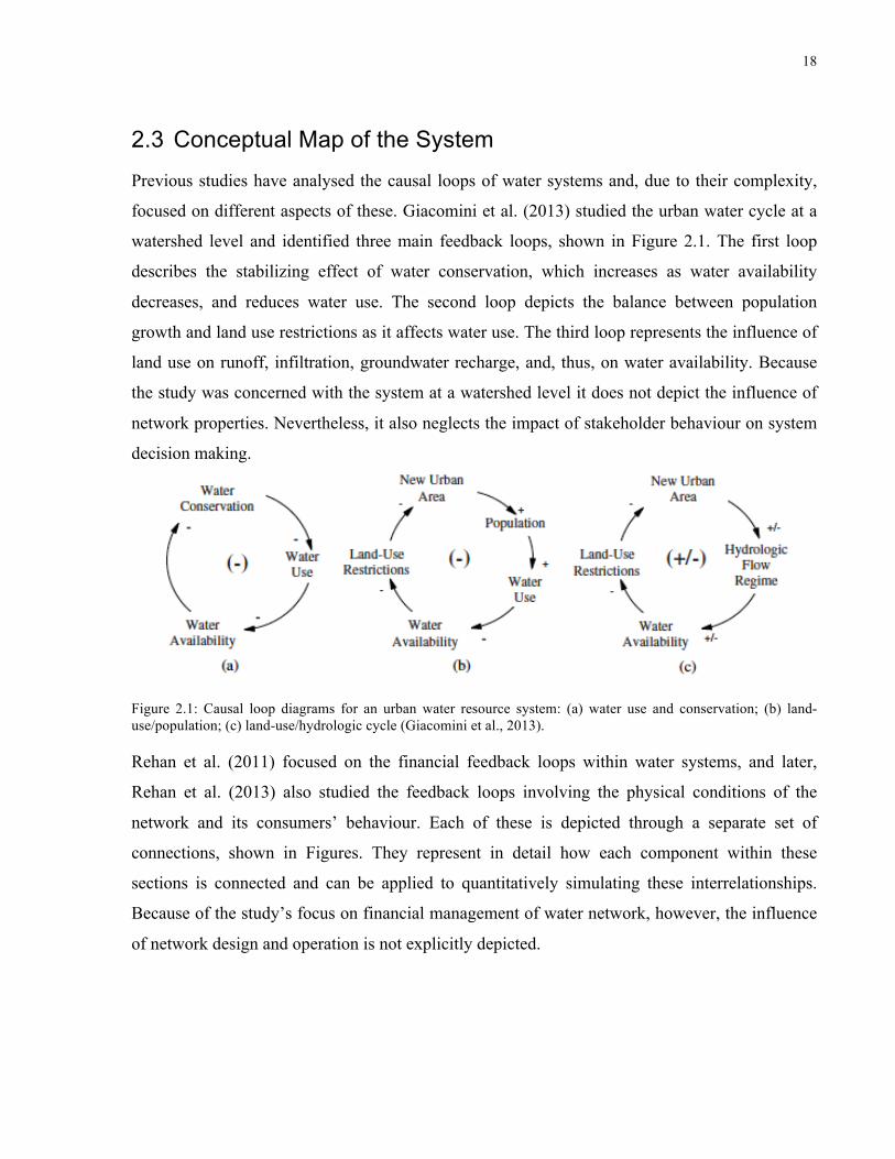
Previous studies have analysed the causal loops of water systems and, due to their complexity,
focused on different aspects of these. Giacomini et al. (2013) studied the urban water cycle at a
watershed level and identified three main feedback loops, shown in Figure 2.1. The first loop
describes the stabilizing effect of water conservation, which increases as water availability
decreases, and reduces water use. The second loop depicts the balance between population
growth and land use restrictions as it affects water use. The third loop represents the influence of
land use on runoff, infiltration, groundwater recharge, and, thus, on water availability. Because
the study was concerned with the system at a watershed level it does not depict the influence of
network properties. Nevertheless, it also neglects the impact of stakeholder behaviour on system
decision making.
Figure 2.1: Causal loop diagrams for an urban water resource system: (a) water use and conservation; (b) land-use/population; (c) land-use/hydrologic cycle (Giacomini et al., 2013).
Rehan et al. (2011) focused on the financial feedback loops within water systems, and later,
Rehan et al. (2013) also studied the feedback loops involving the physical conditions of the
network and its consumers’ behaviour. Each of these is depicted through a separate set of
connections, shown in Figures. They represent in detail how each component within these
sections is connected and can be applied to quantitatively simulating these interrelationships.
Because of the study’s focus on financial management of water network, however, the influence
of network design and operation is not explicitly depicted.

19
Figure 2.2: Feedback loops involving finances of water distribution systems (Rehan et al., 2013).
Figure 2.3: Feedback loops involving customer behavior in water distribution systems (Rehan et al., 2013).

20
Figure 2.4: Feedback loops involving physical conditions of water distribution systems (Rehan et al., 2013).
Another diagram was proposed by Colombo and Karney (2003) seeking to represent the critical
feedback loops in water distribution systems’ operation and performance. Three pillars support
the “labyrinth” of water distribution systems, as coined by the authors: demand, capacity, and
performance. The focus is, thus, on the ability of the system to meet demand requirements.
Although the economic objectives are represented, the influence of stakeholders and system
properties is not shown.

21
Figure 2.5: Causative factors and feedback loops of water distribution systems (Colombo and Karney, 2003).
In order to facilitate the assessment of water distribution system sustainability, the present
chapter proposes another conceptual map of water distribution systems that seeks to more
comprehensively represent the connections of the system qualitatively. It is not all-inclusive but
seeks to illustrate the complexity of the system, particularly with regards to the connections
between the financial, social, and environmental spheres of the systems. Relations between these
are simplified and summarized in Figure 2.6. Three main types of system elements, which
influence the state and characteristics of the system, are distinguished in the map: stakeholders
(in capitals), revenue or costs (in italic), system properties (in bold), and other secondary
characteristics, which stem from these.

22
Beginning with the water source (I), the quality of the water withdrawn, which must be treated to
meet standards set by a governmental regulatory body, affects the cost of treatment. These costs
also depend on the volume of water treated, the sum of user demand and non-revenue water, as
well as the location and type of source (surface or ground water), which influence the cost of
abstraction and import if that is the case. Furthermore, the availability of water, reduced by local
consumption, exports, and natural use to maintain ecosystems, influences stakeholder perception
and willingness to conserve.
The design of the water distribution network (II) is based on what is known and what is expected
to vary in the given context. The local topography, combined with city planning, determine the
elevation differences water will need to overcome, a component in the need for pumping. From a
municipal level, urban planning also defines zoning, i.e. the types and density of users
throughout the network, and the expected population growth, which together stipulate design
demands. Design standards established by the Fire Underwriters Survey in Canada and other
regulatory bodies seek to ensure the safety of the systems through the specification of limits for
pipe diameters, velocities, as well as pressures and flows during normal and emergency
operations.
The time-dependent capacity of this infrastructure to deliver certain flows and pressures under
different conditions depends on the design of the network. The relation between capacity,
operational choices, and real requirements determines how well the network will operate. The
choice of network components (III), their type, material, and dimensions directly affect the
hydraulic parameters of the system, and its greenhouse gas emissions. Specifically for above
ground elements, such as tanks and pumping stations, the aesthetics and location can also affect
user satisfaction.

23
In addition to how the network is designed, the way in which it is operated and controlled (IV)
also affects hydraulic parameters. Operational standards, which are meant to promote safety,
define limits for some of these parameters. The occurrence of hazardous events, such as breaks
and fires, creates sudden change, which impacts operations. Demands rapidly peak, increasing
flow in pipes and dissipation, causing system pressures to drop, sometimes below zero, risking
contamination due to the intrusion of surrounding ground water. In order to improve operations,
data that is collected and analyzed about the system can be used to increase utility knowledge
and feed back into the system.
Figure 2.6: Conceptual map of a water distribution system.
The age and defects of the components of the network, together with the frequency of
maintenance, the hydraulic parameters which indicate the stresses experienced by the system,
and the local conditions (soil, traffic, and climate) which can further undermine the resistance of
(I)Water source
Cost of treatment and abstraction/import
Availability / Scarcity of water OTHER USERS
of water source: cities/ecosystems
Infrastructure capacity
(II)Network design
Design standards(VII)ALL
Stakeholder Paradigms & Expectations
Topography
Water quality standards
Urban Planning
GOVERNMENT (municipal, provincial)
FIRE Underwriters Survey
Operational standards
(IV)System operations
and control
Hydraulic parameters
Quality of water in network
(III)Network components,
Investment in sustainability
programs
USERS
Inquiries and complaints
(V)State of repair
(VI)Total water use
Maintenance frequency
Local Conditions
User Fees
Data available
Water rate structure
Government stimulus funding
and tax base support
Water exports
Maintenance & Repair costs
Salaries and benefits Rehabilitation & Replacement costs
GHG emissions
Risks
UTILITY
STAKEHOLDERSRevenue or Costs
System Properties

24
the system, all influence its state of repair (V). The maintenance frequency established by the
utility, thus, influences maintenance and repair costs, as well as rehabilitation and replacement
costs. The operation of the system generates further costs associated with energy use for
pumping, business activities, general and support activities, as well as management and
supervision.
The state of repair of the network is related to leakage. Higher pressures increase the amount of
water lost, which in turn augments the flow and dissipation in pipes. Therefore, the state of repair
affects hydraulic parameters and vice versa. If, in turn, low dissipation and velocities are
experienced in the pipes, the time of residence of the water increases, affecting the quality of
water within the network. The failure to deliver water according to the flow, pressure, and
quality expected by the users can not only result in inquiries and complaints, causing the utility
to incur costs, but can even generate more serious social costs in the case of damaging or
destructive events.
The amount of water delivered to the users (VI) should meet their reasonable demands. Whether
these demands are strictly necessary is another matter, which can be addressed by investments in
sustainability programs, specifically for conservation and capacity building. Because water
prices are elastic, demands are also affected by pricing. Therefore, if changes are made to the
water rate structure, price-induced-use-changes must be considered in estimating the new
revenue from user fees. Other sources of revenue, depending on the model adopted by the utility,
may include government stimulus funding, tax base, interest, and water exports. The difference
between these and total costs determines the balance of funds available to the utility for future
investments, be they expected or not.
In general, the paradigms and expectations of the stakeholders (VII), government, Fire
Underwriters Survey, utility managers, operators, engineers, water boards, consultants, local
users, and other users, affect all aspects of the system. The perceived benefit of sustainability, be
it reducing consumption, decreasing leakage, or increasing energy efficiency depends on the
combination of infrastructure conditions, quality of services provided, as well as views and

25
values of stakeholders. This perception dictates what is expected of the system and the
willingness to increase its sustainability.
The mapping of these connections, Figure 2.6, facilitates the identification of feedback loops,
instances where the modification of one component causes repercussions that affect that same
element. This relation is displayed between user fees and total water use, hydraulic parameters
and total water use, state of repair and total water use, hydraulic parameters and maintenance
frequency, as well as system operations and data available. For each of these pairs, change is
effected in both directions. The dynamics which give rise to these loops are more complex and
are not described in Figure 2.6 for simplicity.
Another property of the system that can be easily visualized in the conceptual map is the
presence of hubs, elements that are highly connected to the rest of the system. The existence of
various hubs, can complicate the task of mapping, though, since connections intersect and affect
visualization. For instance, the component denominated “all stakeholder paradigms and
expectations” is connected to all stakeholders and affected by all other components of the
system. Therefore, these relations were not mapped in order to avoid confusion. They are instead
meant to be acknowledged as part of that all-inclusive term. Other hubs, which can be identified
in the map are network design and hydraulic parameters.
By following the arrows in the map, the cascade effect of altering one component can also be
traced. Different from a feedback loop, which is a closed circle of connections, a cascade effect
indicates all of the elements affected directly or indirectly by altering one component of the
system. Standards, for example, design or operational, affect greenhouse gas emissions, water
pressure, water quality, leakage, costs, and revenue. The ability to trace causes and consequences
facilitates analysis and can easily inform utilities of indirect connections they might be less
aware of. The identification of these features of the system, feedback loops, hubs, and cascades,
can be used to its advantage. Because they describe how elements are connected to each other,
links can be used to expand positive change over all dimensions of the system.

26
The map, however, does not describe the degree to which each component influences others. A
more detailed, quantitative and qualitative, exploration of these components is required. Whether
for reporting requirements (Ministry of Municipal Affairs and Housing Ontario, 2012 and
Ontario Municipal CAO’s Benchmarking Initiative, 2011) or internal control (City of Toronto,
2012), many utilities collect data on total water use, water use per capita, total costs, total
revenue, infrastructure backlog, leakage, main breaks per km of pipe, and number of household
days with boil water advisories. With these indicators, a preliminary assessment of the system
can be performed, from which certain issues, opportunities, and obstacles can be anticipated. In
order to specify the best solutions, however, more information and analysis is needed.
The complexity of water distribution systems and their multi-objective nature evidence the need
for multiple approaches in increasing their sustainability. In order for these approaches, such as
pipe rehabilitation, pump rescheduling, rate changes, conservation, etc., not to cause
complications due to unforeseen feedbacks, they must consider the connections within the
system. The decision support tools proposed in the following chapters investigate and seek to
leverage connections within water distribution systems in order to increase their sustainability.
The principal connections analyzed or touched upon in each chapter are as follows:
• land use, demographics, and water consumption (chapter 3);
• stakeholder expectations and utility strategies (chapter 4);
• network design, operations, and energy efficiency (chapter 5);
• network design, operations, and infrastructure performance (chapter 6), and;
• network design, water demands, risks, and system costs (chapter 7).
The present chapter has described some of the multiple definitions of sustainability and how they
are applied to the assessment of water distribution systems. It is argued that the various
connections between objectives of sustainable systems call for integrated approaches that not
only acknowledge these relations but also take advantage of them. Accordingly, water system

27
connections were mapped, facilitating the visualization of feedback loops, hubs, and potential
cascade effects.

28
3 Integrated Database for Demand Management Amongst the connections explored in chapter 2, are those that influence water demands. User
characteristics have been shown in previous studies to be correlated to water use and have been
applied in demand forecasting. The present chapter, instead, applies this information to demand
management. It integrates water use, land use, and demographic data from three Ontario
municipalities and defines key metrics, charts and benchmarks for comparison, targets for
conservation, and clusters of users.
Albeit available to many North American utilities, this data is seldom explored by these,
particularly in the context of demand management. Nevertheless, the impending water scarcity in
certain regions and high costs of system expansions, increasingly motivate water conservation.
Accordingly, the municipalities of Barrie, Guelph, and London, ON agreed to participate in the
present study and receive actionable information regarding water demand.
This chapter is based on the paper entitled “Building an Integrated Water–Land Use Database for
Defining Benchmarks, Conservation Targets, and User Clusters” by Rebecca Dziedzic, Katelyn
Margerm, Jeff Evenson, and Bryan Karney published in the Journal of Water Resources
Management and Planning and reproduced herein with permission from ASCE. The objective
of this chapter is to guide utilities in using data that is already available to better describe their
users and target conservation. Doing so, it addresses the issues of water scarcity, high expansion
costs, and lack of customer information.
3.1 The Value of Integrating Data
“Divide and conquer”, specialization, is a common motto in solving complex problems, which
splits complex realities into a variety of disciplines, sectors, departments, etc. This means,
however, that interactions and synergies between the segments are either ignored or downplayed.
According to Hussey and Pittock (2012), three major barriers prevent greater integration between

29
sectors and policy domains: data deficiencies (missing or disorganized), weak existing policies
and frameworks (fragmented, inconsistent, lacking review), and cultural inertia/path-dependency
(silo mentality). A consistent system for collecting data in an easily retrievable, standardized, and
comprehensive fashion is instrumental in managing water demand (Cahill and Lund, 2013). The
present study focuses on data as a pathway to resolve the second and third types of barriers. It
integrates water, land-use, and demographic data with the objective of facilitating both
understanding and demand management.
The United Nations Environmental Programme (2012) reviewed worldwide applications of
integrated approaches to water resource management and recognized the need for better
information management, stating that “Information is the foundation of good decision-making
and planning”, with reference to integrated water resources management in Agenda 21 (United
Nations Conference on Environment and Development, 1992). Although progress has been slow
(Muste, 2013), this type of effort has been facilitated in recent years due to advances in
technology and information exchange, fostering a greater commitment to initiatives in data
collection (Maidment, 2008). Bringing together data from different disciplines fills in gaps of
information and knowledge (Muste, 2013).
Boyle et al. (2011) stress the fact that utilities already have valuable data at hand. Utility billing
data can be used to inform many types of management decisions, such as pricing, conservation
marketing, and peak planning. The use of this data is supported by three characteristics: it is
available to all utilities; it can be used to target specific customer groups with customized
messages that are more cost-effective than broad public outreach programs; and it can enable an
understanding of specific customers, leading to localized utility policies and strategies.
Using more detailed data can provide utilities with greater insights on to how water is consumed
over space and time (Polebitski and Palmer, 2010). Jorgensen et al. (2009) indicate that
demographics, dwelling characteristics, and household composition all directly impact water
consumption, conservation intention, trust, perceived behavioural control, perception, and habits.
Polebitski and Palmer (2010), as well as Morales et al. (2011) joined utility billing data with

30
census demographic and property appraisal data to forecast residential and non-residential water
use, respectively.
Shandas and Parandvash (2009) suggest that, given current population growth and urban
development, approaching water use through the lens of urban planning, namely the structural
and demographic drivers of consumption, can improve the effectiveness of water conservation.
Brooks (2006) defines water demand management operationally according to five motivators: (1)
reducing the quantity or quality of water required for a specific use; (2) adjusting the nature of
the task so it can be accomplished with less or lower-quality water; (3) reducing loss in quantity
or quality of water in the distribution system; (4) shifting time of use to off-peak periods; and (5)
increasing the system’s ability to operate during droughts. Other benefits include deferring and
reducing capital works, reducing pumping costs, and increased flexibility of demand-side
solutions in adjusting to changing circumstances (Sahely and Kennedy, 2007). Although water
demand management can, thus, be multifaceted, the focus here is on conservation.
The Ontario Water Works Association (2006) proposes a method for decreasing demand, which
begins with evaluating the system and setting goals. Guidelines include the installation of certain
efficiency devices towards the reduction of consumption by a preset percentage.
Recommendations for selecting the strategy and target, however, are not given and may be
arbitrarily determined by the utility. Morton (2011) suggests establishing a best practice range
instead. According to the Morton (2011), there are two objectives in developing a benchmark:
(1) determining the appropriate metric to be used, e.g. m3.m-2.yr-1, L.cap-1.day-1, and (2)
determining the benchmark value based on the water consumption intensity across the dataset.
The best practice range can be defined as a percentile, such as the first quartile of the dataset.
Data mining is, thus, instrumental in establishing benchmarks for different sectors and
monitoring improvement.
Dziegielewski and Kiefer (2010) suggest normalizing metrics for comparability. If metrics are
being compared for a single utility over time, it should be sufficient to adjust the calculated
metrics for weather conditions, temperature and rainfall. Annual changes in the number of users
31
are accounted for by the scaling variable, such as population or building space. When metrics are
compared across different utilities, it is recommended that all external factors that influence
water consumption (outside the control of water users) should be considered. However, it is
acknowledged that normalization of weather and other confounding factors across different
utilities can be problematic. A practical approach is to use metered account-level information for
homogeneous groups of customers and the same dimensions of water use (e.g. total annual,
seasonal, non-seasonal).
Even though targets may not currently be set across utilities, provincial or national averages
provide an important basis for comparison in a larger, yet similar, stage. Environment Canada
(2010), from a survey of 530 Canadian municipalities, presents water use rates by province.
Average residential flow in Ontario is approximately 267 L.cap-1.day-1, almost 20% lower than
the national value of 327 L.cap-1.day-1. Maas (2009) offers a blueprint for a comprehensive water
conservation strategy, in which a target of 150 L.cap-1.day-1 for Ontario municipalities is
suggested. Albeit not at a policy level, this has been accepted by many Ontario utilities as a
suitable goal. This target is inspired by the “Target 140” campaign from Queensland, Australia,
where water use was reduced from 300 to 140 L.cap-1.day-1. According to preliminary estimates,
the goal of 150 L.cap-1.day-1 could be achieved passively, simply by installing high efficiency
fixtures and appliances in all new homes and point of sale transactions. Therefore, there is clearly
potential for further conservation, the feasibility of which will depend on current demands,
policies, consumer behaviour, and utility engagement.
Benchmarks for industrial, commercial, and institutional (ICI) water use are harder to find, since
there is more variation, especially between different types of industries. Therefore, water use
data must be sorted according to property codes or industrial classification codes for better
comparisons. Gleick et al. (2003) present water use benchmarks for different industries in
California by sector, specifically by Standard Industrial Classification codes. Water consumption
is normalized by production or number of employees. South East Water (2006) provides an
extensive list of benchmarks per sector based on surveys and literature review. The dates of the
references, however, vary between 1997 and 2006, suggesting some of the data may no longer be

32
current or relevant. The rate of obsolescence will depend on the sector, acceptance of these
targets and potential for improvement.
Previous research, as noted above, has stressed the need for conservation planning and
underlined the importance of integrated approaches that combine information from different
areas to fill in gaps of knowledge. Using practical models, with input variables that can be
collected, monitored and used by the utility is key (Donkor et al., 2014). The present study
integrates data that is readily available to most Canadian municipalities and their water utilities:
water billing records, demographic census information, and structural data from property tax
assessments. This information is used to build an integrated database to support decision-making,
specifically demand management. Accordingly, benchmarks, conservation targets, and user
clusters are defined.
3.2 Methodology
The data mining method, on which this study is based, comprises six steps: problem definition,
data preparation, data exploration, modeling, evaluation, and deployment. This process was
repeated for three Ontario municipalities, and results were compared. The problem definition
frames the succeeding steps by describing study objectives. Data preparation encompasses the
process of cleaning and formatting the data, as well as building the integrated database. In data
exploration, distributions, trends, and metrics are assessed and compared. The first benchmarks
as well as targets for conservation are also established in this phase. Modeling furthers the
analysis as user clusters are defined. These results are then evaluated and the model built for data
clustering can be applied to different data sets.
3.2.1 Problem Definition
Many water utilities, such as the ones studied herein, bill their customers according to general
sectors, i.e. residential, industrial, commercial, and institutional, or even at a flat rate for all
users. Although Canadian municipalities have access to land use and demographic data from the

33
Municipal Property Assessment Corporation (MPAC) and Statistics Canada (Statcan),
respectively, most utilities only distinguish users by billing class. This classification is not
descriptive, and does not allow for the definition of homogeneous groups of users, which are
more suitable for analyzing trends, establishing benchmarks, and targeting conservation.
Nonetheless, the more than 100 classes used by MPAC may prove to be excessive for utility
needs, especially if different strategies are being used for each different type of consumer.
Accordingly, the study seeks to define benchmarks and targets for water conservation, as well as
water user segments in three Canadian municipalities, Barrie, Guelph, and London, based on
integrated water consumption, land use, and demographics data.
3.2.2 Data Preparation
The integrated databases were created by connecting data from an SQL server, through ODBC
(Open Database Connectivity), for easy storage and updating. Database construction was
completed as part of a research project funded by the Ontario Ministry of Environment with the
Canadian Urban Institute (CUI). Cleaning and formatting of the billing records was
subcontracted. This involved joining data from different months, and updating or rectifying
inconsistent customer identifier or address formats. Spatial data, relating addresses to roll
numbers, parcels, and dissemination blocks was joined by the CUI using their geographic
information system (GIS) data. Roll numbers are the property identifiers used by MPAC for tax
assessments. Parcels are pieces of land, generally equivalent to properties, and dissemination
blocks, equivalent to city blocks, are the smallest geographic areas for which Statcan releases
population counts.
The integration of water consumption, land use, and demographic data involved connecting
information from four different sources: water utilities, MPAC, Statcan and CUI.
Six tables were generally integrated in the database, with their primary variables listed below,
either as categorical (c), or numerical (n):
• Customer Information (utilities): Customer ID (c), Address (c), Rate Class (c);
34
• Billing Data (utilities): Customer ID (c), Monthly Water Consumption (n);
• Address Table (CUI), created using a series of spatial joins in GIS: Address (c), Roll
Number (c), Parcel ID (c), Dissemination Block (DB) ID (c);
• Structural Data (MPAC): Roll Number (c), Year Built (n), Building Footprint (n),
Property Code (c);
• Parcel Data (utilities): Parcel ID (c), Parcel Area (n), Building Area (n);
• Demographic Data (Statcan): Dissemination Block ID (c), Population Count (n).
Customer information and billing data are collected for each user, with Customer ID as the
unique identifier. Billing data between 2006 and 2011 was collected. These datasets were linked
by Customer ID, and then summarized by address so that they could be combined with the
address table. After these were joined, water consumption was associated with roll numbers,
parcels, and DBs, and can, therefore, be integrated with land use and demographic data. After
summarizing by roll number, this data was combined with the structural data. This was then
summarized, either by parcel or by DB, to be joined to the parcel or demographic data,
respectively.
There are, thus, two primary tables as outputs of this integration process: a parcel table, with
water and land use at the parcel level, and a DB table, with water, land use, and population count
by DB. This can then be mapped, facilitating the visualization of spatial trends. Guelph, the
smallest of the three municipalities had approximately 120,000 inhab. in 2011, distributed in
35,000 parcels. Barrie had 150,000 inhab. and 42,000 parcels (generally equivalent to
properties), while London, more populated, had 360,000 inhab. in 99,000 parcels.
Data integration can be a cumbersome process if attention is not paid to differences in
formatting, missing values, data inconsistencies, non-unique identifiers, and varying levels of
data summarization. That being the case, it is helpful to sketch the integration process
beforehand and name queries and tables in a simple, yet descriptive, manner. In addition, after
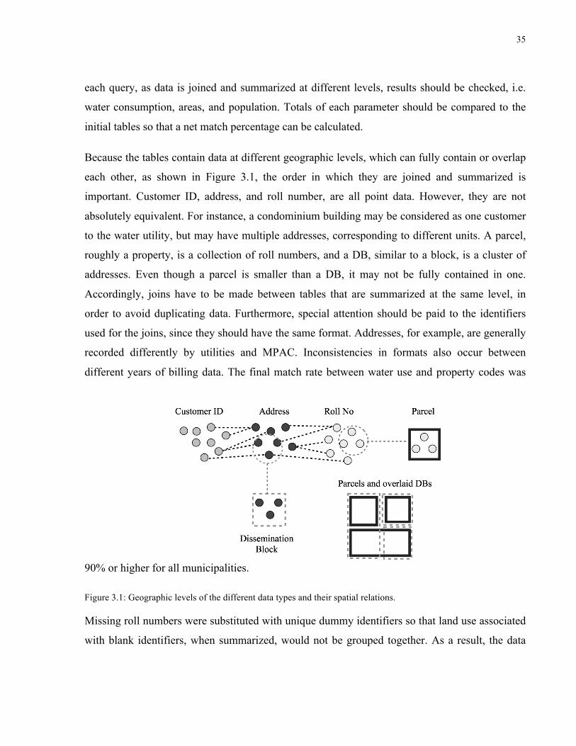
35
each query, as data is joined and summarized at different levels, results should be checked, i.e.
water consumption, areas, and population. Totals of each parameter should be compared to the
initial tables so that a net match percentage can be calculated.
Because the tables contain data at different geographic levels, which can fully contain or overlap
each other, as shown in Figure 3.1, the order in which they are joined and summarized is
important. Customer ID, address, and roll number, are all point data. However, they are not
absolutely equivalent. For instance, a condominium building may be considered as one customer
to the water utility, but may have multiple addresses, corresponding to different units. A parcel,
roughly a property, is a collection of roll numbers, and a DB, similar to a block, is a cluster of
addresses. Even though a parcel is smaller than a DB, it may not be fully contained in one.
Accordingly, joins have to be made between tables that are summarized at the same level, in
order to avoid duplicating data. Furthermore, special attention should be paid to the identifiers
used for the joins, since they should have the same format. Addresses, for example, are generally
recorded differently by utilities and MPAC. Inconsistencies in formats also occur between
different years of billing data. The final match rate between water use and property codes was
90% or higher for all municipalities.
Figure 3.1: Geographic levels of the different data types and their spatial relations.
Missing roll numbers were substituted with unique dummy identifiers so that land use associated
with blank identifiers, when summarized, would not be grouped together. As a result, the data

36
can remain linked to its address despite the lack of a roll number. Because population counts are
only released every four years, and water consumption data is reported monthly, demographic
data was interpolated for the years with no census data, and only yearly per capita metrics were
calculated. Population was assumed to increase geometrically. Land use data is also not released
yearly. In this case, if the year built is more recent than the year of consumption, building
footprint and unit (address) count were assumed to be zero. Whenever consumption was null,
records were also neglected. Outliers (over three standard deviations away from the mean) were
also removed before the modeling phase, represent 2% or less of entries. If unit count, building
space, or property area were missing, values were modeled based on similar users with the
nearest neighbour algorithm.
Water consumption data is collected every billing cycle, which is either monthly or bi-monthly
for the given municipalities. However, different parts of the cities are metered at different times
of the month. Therefore, attention must be paid to the difference between reading date and billing
date, especially when seasonal use is being calculated. Although two regions may have been
billed at the same time that does not mean that the billed water consumption corresponds to the
same period for both. The analyzed water data was separated by billing date, although seasonal
use was calculated differently based on the billing cycle of the user.
3.2.3 Data Exploration
Because of this study’s emphasis on integrating data, the amount of data and specific interest of
the cities in visualizing correlations and targeting conservation, the data exploration focused on
bivariate analyses. The primary variables that were analyzed in this phase were monthly water
use (m3), unit count, building footprint (m2), year built, property area (ha), population (cap), rate
class, and property code. A spreadsheet-based summary tool comparing metrics from all three
cities was developed for the communication of results to water utilities, and for use in both result
assessment and conveying this information to policy makers, and users. When sharing these
results outside the organization, however, care should be taken to avoid disclosing individual
information. This implies classifications may have to be grouped, and if data is being mapped,
individual properties should not be able to be singled out.

37
The summary tool graphically represents relations between user characteristics and demand,
temporal (monthly, seasonally, and annually) trends of water use, as well as variations within and
between water use metrics in property classes and sectors. It, thus, addresses questions regarding
the significance of user characteristics to demand management, expectations of future use given
changes to these characteristics, and key user types to target for conservation. The tool is most
helpful to utility managers and planners, who can easily view and extract summarized
information to plan conservation strategies and communicate with stakeholders.
The summary tool comprises three major components: distributions, trends, and metrics. The
first two present charts of total water use, whereas the latter has various metrics of normalized
water consumption. The distribution of water consumption is presented in pie charts by sector
and property code, as well as bar charts of the top water-consuming property codes, the
percentage of total water use they represent together with the class coefficient of variation of
normalized water consumption. Some examples of figures provided in the tool and the types of
conclusions obtained are shown in the results section.
3.2.4 Modeling Given the objective of creating water user segments, the modeling phase applied different
clustering techniques in grouping the data. Segments were created within each of the four larger
sectors: residential, industrial, commercial, and institutional. Furthermore, for this process to be
easily replicable and results compared with other utilities, property codes were clustered through
three methods: hierarchical clustering, K-means clustering, and self-organizing maps. According
to Vesanto and Alhoniemi (2000), using prototype clusters reduces computational effort and
noise since the prototypes are local averages of the data. The same methods were applied without
using the property codes as cluster prototypes, and the results compared. Data mining software
with a user interface was used to facilitate the visualization and understanding of the process, as
well as its modification.
Through a principal component analysis, in which water consumption was set as the target and
population count, unit count, building space, and property area as attributes (components), it was

38
found that all components equally explain the variations in water use. Population count was only
included in the analysis of the residential sector, since it is an indicator of residential occupancy,
not ICI. The attribute with the highest importance varies between sectors and cities. Correlations
between the three parameters for ICI vary, generally resulting above 0.5, and reaching 0.95 in
some instances. Because these correlations are not consistent, and occasionally low, no attributes
were considered sufficiently similar to be excluded from the modeling phase for ICI. Population
count, in the residential analyses, presented higher correlations with the other attributes - at least
0.7, and up to 0.99. Therefore, only unit count, building space, and property area were kept in the
residential clustering as well.
The first clustering technique applied, hierarchical agglomerative clustering, minimizes the
linkage, dissimilarity within clusters. The algorithm is initiated with the data points as individual
clusters, which are progressively merged at each step. This requires defining a type of
dissimilarity. Ward’s linkage, which minimizes total within-cluster variance based on weighted
square distance between cluster centers, was used. The distance between two clusters is defined
as the increment in the sum of squares if these two are merged, as shown in (3.1)
Δ A,B( ) = xi −mA∪B
i∈A∪B∑
2−
xi −mA
i∈A∑
2−
xi −mB
i∈B∑
2=nAnBnA + nB
mA −
mB
2 (3.1)
where mj is the center of cluster j, and nj the number of points in it. At each iteration the pair of
clusters with the minimum linkage are merged. This process continues until merging costs jump
or the number of cluster becomes too small.
K-means, the second method, assigns a specified number of centroids to the data set and
minimizes the total intra-cluster distance (Tan et al., 2006). The number of clusters was
optimized according to the silhouette index (3.2), which relates the average distance between a
point and all other points within its cluster (3.3), as well as between the point and all points in
other clusters (3.4). This approach generally outperforms other internal indices, and its
performance is close to that of the best relative indices (Brun et al., 2007).

39
S(x) = b(
x)− a(
x)
max b(x),a(
x)"# $%
(3.2)
a( x) = 1n j −1
d( x, y)y∈C j ,
y≠x
∑ (3.3)
b( x) = mink=1,..,J ,k≠ j
1nk
d( x, y)y∈Ck
∑$
%&
'
()
(3.4)
where S( x) is the silhouette index, a( x) the average distance between x and all other points in
cluster Cj, b(x) the minimum of the average distances between x and the points in the other
clusters, d( x, y) the distance between points x and y. The Euclidean distance (3.5) was applied
as the objective function for the K-means clustering, as recommended by Xu and Wunsch
(2009).
d( x, y) = xl − yl1 2
l=1
L∑#
$%
&
'(2
(3.5)
where l is the dimension of the data point.
In the third method, self-organizing maps, each node of data is connected to a vector by a
specific weight, which defines the cluster. Adjusting the weights (3.6) minimizes the distance
between clusters, and the learning rate (3.7) decays at each iteration (Vesanto and Alhoniemi,
2000).

40
wrt+1 =wrt +Δwrt =wrt +γ r
t xi −wrt( ) (3.6)
γ rt =α tvr
t (3.7)
where wrt is the vector of weights for neuron r, γ r
t the learning rate, α t is the value of the global
learning rate, and vrt the neighbourhood kernel. In order to observe the self-organization
property, the neighbourhood factor must be a decreasing function of the grid distance between
the best matching unit and the neuron being adapted. The best matching unit is defined as the
closest neuron to the input.
The Gaussian function was applied for calculating the neighbourhood kernel, as recommended
by Lee and Verleysen (2002) to produce better results than the Bubble function. The latter is a
discrete function, the kernel is either 1 when the grid distance is less than the neighbourhood
radius or 0 if it is greater than the radius. The Gaussian kernel is a decreasing exponential
function of the grid distance.
vrt = exp −0.5 d(u,r)
λ t"
#$
%
&'
2(
)
**
+
,
-- (3.8)
where d(u,r) is the distance between the best matching unit u and the neuron r, and λ t is the
neighbourhood radius. The size of the map and the radius were selected so as to generate a small
number of clusters, similar to what was found with the application of the two other methods.
Hillenmeyer (2005) points out issues for each of the three clustering methods. The hierarchical
agglomerative algorithm is sensitive to outliers and might not produce optimal results, if a local,
instead of a global minima is found. Additionally, the generated trees might be too complex and
hard to interpret. K-means clustering is a faster method. Nonetheless, results are sensitive to the
choice of initial seeds. Self-organizing maps can be easier to visualize. However, the solution is
sensitive to the starting structure, and there is no guarantee of convergence to representative
41
clusters. These methods were not only applied to clustering the property codes and their average
metrics, but to the parcel data (i.e., water use at property level) as well. In this case, due to the
number of data entries, only a sample was used to create the clusters.
3.2.5 Evaluation
The results were compared among the three cities, for cross-validation, between the different
clustering methodologies, and with or without property codes as the initial clusters. Clusters were
validated internally with the pseudo-F statistic, proportional to the ratio between the sum of
squares between clusters, and the sum of squares within clusters. For external validation, the
Rand statistic was used in comparing the clusters created with parcel level data and property
codes. The Rand statistic measures the proportion of pairs of vectors that agree by belonging
either to the same cluster and property code or to different clusters and property codes (Brun,
2007). It can vary between 0 and 1, with 1 being the highest score.
3.2.6 Deployment
In order to update the clusters with more recent data or model consumption in other
municipalities, the data would need to be prepared, links in the database updated or modified,
and queries rerun. With this, a new input file for the modeling stage would be created. Since the
models will be run in a data mining software, deployment will use the same schemas created for
modeling. For the evaluation of the clusters through the pseudo-F and Rand statistics, a program
was written.
3.3 Results
Residential water use represents more than 60% of total consumption in all three municipalities,
combined. The averages of the three cities are presented in Figure 3.2. Overall, approximately
5% of the total water consumption was not assigned a property code in the database, due to
formatting issues or outdated property information. Based on a search of the addresses of a
sample of users with unassigned property codes, these were found to be from the ICI sectors.
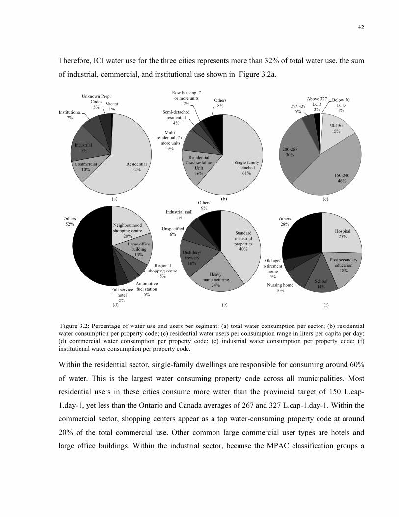
42
Therefore, ICI water use for the three cities represents more than 32% of total water use, the sum
of industrial, commercial, and institutional use shown in Figure 3.2a.
Figure 3.2: Percentage of water use and users per segment: (a) total water consumption per sector; (b) residential water consumption per property code; (c) residential water users per consumption range in liters per capita per day; (d) commercial water consumption per property code; (e) industrial water consumption per property code; (f) institutional water consumption per property code.
Within the residential sector, single-family dwellings are responsible for consuming around 60%
of water. This is the largest water consuming property code across all municipalities. Most
residential users in these cities consume more water than the provincial target of 150 L.cap-
1.day-1, yet less than the Ontario and Canada averages of 267 and 327 L.cap-1.day-1. Within the
commercial sector, shopping centers appear as a top water-consuming property code at around
20% of the total commercial use. Other common large commercial user types are hotels and
large office buildings. Within the industrial sector, because the MPAC classification groups a
Hospital 25%
Post secondary education
18%
School 14% Nursing home
10%
Old age/retirement
home 5%
Others 28%
Vacant 1%
Residential 62%
Commercial 10%
Industrial 15%
Institutional 7%
Unknown Prop. Codes
5%
Single family detached
61%
Residential Condominium
Unit 16%
Multi-residential, 7 or
more units 9%
Semi-detached residential
4%
Row housing, 7 or more units
2% Others
8%
Neighbourhood shopping centre
20%
Large office building
13%
Regional shopping centre
5% Automotive fuel station
5% Full service
hotel 5%
Others 52%
Standard industrial properties
40%
Heavy manufacturing
24%
Distillery/brewery
16%
Unspecified 6%
Industrial mall 5%
Others 9%
Below 50 LCD 1%
50-150 15%
150-200 46%
200-267 30%
267-327 5%
Above 327 LCD 3%
(a) (b) (c)
(d) (e) (f)

43
variety of different industries under one property code, standard industrial properties, only
general information is available. The more informative denominations show the high water
consumption of specific uses, such as distilleries or breweries and water treatment stations. In the
institutional sector, health and educational facilities use the most water. Due to their high
combined water use, these categories of water users are prime targets for water conservation
programs.
Figure 3.3: Yearly and seasonal residential water consumption trends from 2006 to 2011: (a) total use in London; (b) total use in Barrie; (c) total use in Guelph; and in all three cities (d) use per capita; (e) use per hectare; and (f) use per unit.
0
50
100
150
200
250
300
350
2006 2007 2008 2009 2010 2011
L.c
ap-1 .d
ay-1
London Barrie Guelph
0
1
2
3
4
5
6
7
2006 2007 2008 2009 2010 2011
106 .
m3 .y
r-1
Annual Winter Summer
0
500
1000
1500
2000
2500
2006 2007 2008 2009 2010 2011
m3 .h
a-1.y
r-1
London Barrie Guelph
(c) (d)
(e) (f)
0
5
10
15
20
2006 2007 2008 2009 2010 2011
106 .m
3 .yr-1
Annual Winter Summer
0
2
4
6
8
10
2006 2007 2008 2009 2010 2011 10
6 . m
3 .yr-1
Annual Winter Summer
(a) (b)
0
50
100
150
200
250
300
350
2006 2007 2008 2009 2010 2011
m3 .u
nit-1
.yr-1
London Barrie Guelph

44
A decrease in residential consumption, from 2006 to 2011, was observed for all three cities,
Figure 3.3a, b, and c. Despite the increase in population, gross water use decreased in these cities
due to higher water rates as well as an increased focus on conservation, through consumer
education, rebates for high efficiency fixtures and appliances, or outdoor water use programs.
The rates of decrease in per capita consumption are similar for all three cities. Residents have
been reducing their water usage to such a degree, that it counteracts the increase in population.
Different trends, however, were observed for low, medium, and high density dwellings. There is
also a reduction in water use for more recent building vintages, Figure 3.4. The trends are shown
on different scales for each municipality in order to facilitate the visualization of the seasonal
components. Values for the city of Barrie were extrapolated from 2009 and 2010 data because of
issues in formatting the billing records. Residential water use during the winter remained fairly
constant for all cities. The variation in yearly consumption, is thus, greatly explained by higher
summer (peak) water use. Note that summer and winter each correspond to three months of
consumption and their sum does not equal yearly water use.
Residential consumption per unit, Figure 3.3f, has also decreased, although less intensely than
per capita, Figure 3.3d, suggesting there are now more residents per unit in these cities. Trends in
water use per building space, not shown, are very similar to those per unit. Consumption per
property area has generally decreased as well. For all three cities, residential trends in m3.ha-1,
Figure 3.3e, are similar to those simply in m3, Figure 3.3a to c. Therefore, property area does not
explain the variation in residential water use over time, but represents water use density. These
trends are instrumental in planning, for forecasting future demands, as well as costs and revenue.
0
50
100
150
200
250
Prior 1941 1941-1976 1976-1996 1996-2006 2006 to present
L.c
ap-1
.day
-1
London
Barrie
Guelph

45
Figure 3.4: Residential water consumption per capita by building vintage for Barrie, Guelph, and London.
Figure 3.5 displays two important characteristics of targets for conservation: high water use,
indicating a greater significance of the particular user type to the overall system, and potential for
markedly decreasing total consumption, given the cumulative effect of various small
modifications; and high variation of water use metrics (m3.m-2 or m3.unit-1) within the class,
evidencing the potential for improving practices. Only top water using property codes in Barrie
are shown in Figure 3.5 as an example. In all three cities, within the residential sector, target
property codes for conservation are single-family households, multi-residential units,
condominium units, and row houses. Within the ICI sectors, targets are hospitals, shopping
centers, schools, and restaurants. Because industrial property codes are less detailed, and
different property types are grouped, it is more difficult to pinpoint targets. By identifying
specific property types, communication regarding conservation programs can be tailored to
emphasize particular efficiency devices or practices.
0
0.5
1
1.5
2
2.5
0%
10%
20%
30%
40%
50%
Sing
le fa
mily
det
ache
d
Mul
ti-re
side
ntia
l, w
ith 7
or m
ore
units
Free
hold
Tow
nhou
se/R
ow h
ouse
Res
iden
tial C
ondo
min
ium
Uni
t
Nei
ghbo
urho
od sh
oppi
ng c
entre
Sem
i-det
ache
d re
side
ntia
l
Hos
pita
l, pr
ivat
e or
pub
lic
Stan
dard
indu
stria
l pro
perti
es
Indu
stria
l mal
l
Scho
ol
301 340 309 370 430 311 621 520 580 605
Coe
ffic
ient
of V
aria
tion
% o
f Tot
al W
ater
Use
% Total
Coef. Variation

46
Figure 3.5: Percentage of total water use and coefficient of variation of water use metrics for the largest water using property codes in Barrie, ON, Canada.
Given the detailed, parcel or DB level, water consumption data for sectors and property codes,
benchmarks can be determined for each. As recommended by Morton (2011), benchmarks were
defined as the 25th percentile for each group of users, a convention that accounts for the level of
water consumption and user distribution. The frequency of the metrics is calculated according to
their denominator, i.e. building space, unit count, property area, or population. For instance, the
resulting benchmarks for residential consumption per capita are 172 L.cap-1.day-1, 149 L.cap-
1.day-1, and 156 L.cap-1.day-1 in London, Barrie, and Guelph, respectively. Naturally, as
conservation ensues, benchmarks will change, motivating continuous improvement.
Clustering of parcel level data indicated that users under the same property code tend to group
together, i.e., they have similar water use metrics. Therefore, users in the same class, expected to
demand water for the same end-uses, yet at different intensities, were shown to consume water
similarly at the individual or building area level. However, there is not a clear separation between
property codes. Only two to five clusters were formed within each sector, whether the process
was initiated with parcel data or property codes. According to the pseudo-F statistic, hierarchical
and K-means performed similarly for clustering parcel level data. K-means performed the best in
clustering property codes. Based on the Rand statistic, the hierarchical algorithm produces parcel
clusters that best match property codes. In the residential sector, hierarchical clustering generated
the best clusters as evaluated by the pseudo-F, and those most similar to property codes,
according to the Rand statistic. The highest Rand values among all sectors were found for the
residential clusters, between 0.94 and 0.96. This, however, is also due to the fact that one
property code, single family dwellings, represents more than half of residential users.
Clusters of the parcel data of the ICI sectors correlated less to the property codes, since water use
varies more in these classes, and the distribution of the metrics is more scattered. Values varied
from 0.4 to 0.7, depending on the sector and the municipality. Although data was clustered at the
property level in order to compare to the property code prototype clusters, data was still
separated by sector. This distinction, however, was not confirmed by another cluster analysis, in

47
which sectors were not separated in the input data. Although parcel data from identical property
codes tend to cluster, sectors are not segregated through clustering. Therefore, separating water
users into sectors does not reflect an inherent divide of the data, but facilitates user
understanding.
Because the municipalities are composed not only of different property codes but users that
consume water at different levels, the clusters formed for each city differ. Although clusters
differ, in all three cities, similar property codes tend to cluster, such as different types of multi-
residential buildings, restaurants, shopping centers, hotels, retail stores, and nursing or retirement
homes. Furthermore, within each sector a large cluster was formed, with different property
codes, yet similar water metrics, and a few smaller clusters clusters with similar types of
properties. These smaller clusters, formed in one or more of the three cities, are listed below and
whether their water use metrics are higher (h) or lower (l) than the other users in the “catch-all”
cluster:
• Residential: residential properties with 3 or more self-contained units (h), cooperative
housing (h), condominium units (l), other residential properties;
• Commercial: restaurants (h), shopping centers (h), hotels and motels (h), banks and
similar financial institutions (l), retail (l), other commercial properties;
• Industrial: heavy non-automotive manufacturing (h), automotive (h), private generating
stations (h), water, wastewater, and waste treatment plants (h), distilleries and breweries
(h), other industrial properties; and
• Institutional: hospitals (h), retirement and nursing homes (h), ambulance and police
stations (h), museums and art galleries (h), other institutional properties.

48
3.4 Discussion
The method described herein for integrating water, land use, and demographic data is based on
the data available to Canadian water utilities. However, it can be replicated for any utility where
this data is collected. For those utilities which do not have access to such information, or which
are beginning to plan their database, this study can assist in understanding the usefulness of
different types of data, and determining which information should be collected. Altogether the
study advocates a departure from the idea of simply collecting the maximum amount of
information about the system, to instead collect data that can support measures for system
improvement.
Data preparation, as was the case in the present study, can be the most time consuming step of
the data mining process, especially when integrating information from different sources. Data
was provided at different spatial levels and in different formats. Because this type of research
was not the application initially envisioned for the data, steps were not taken by the different data
providers towards improving integration. A consensus between different providers would greatly
facilitate the process. There should be a realization that data is not confined to sectors, and the
exchange of information between departments and organizations is invaluable. Information
should, thus, be collected and maintained accordingly. Data should be easily understood by
whoever may work with it. Therefore, future databases should evolve to be interoperable.
Based on the difficulties faced in the present work, some recommendations for integrating data
are:
• Request a list of identifiers of the data that is to be purchased;
• If subcontracting any part of the process, be clear and specific about the procedure and
expected results, since the employed professional might be an expert in data mining, but
not water demand management;
• Sketch the structure of the database, input data, joins, queries, and output data, and update
as needed;

49
• Define a descriptive nomenclature for the components of the database;
• Ensure data is formatted consistently throughout;
• Check match rates for each join or query;
• Summarize data to the desired spatial level, before joining; and
• Keep a log of issues encountered.
The applied clustering techniques divided the water users in all sectors into one large group and
two to four smaller groups with similar property codes. This distinguishes high or low water
using clusters, which is instrumental in selecting targets for conservation. In order to better
understand the segments of users, especially those grouped under one large cluster, and create
more detailed clusters, further information could be added to the database, such as:
• Unit counts for all multi-unit residential buildings;
• Unknown property codes;
• Standard Industrial Classification codes which are more detailed than property codes;
• Participation in conservation programs;
• Fixture counts;
• Building or plumbing inspections;
• Temporary residents;
• Water metering; and
• User income.

50
Because the clustering analysis indicated that users under the same property code or similar
property codes tend to cluster together, if utilities do not have other, more detailed, information
available, these can be used to define segments of water users. This is particularly relevant for
improving customer messaging and water rate structures which currently only distinguish
between sectors: residential, industrial, commercial, and institutional.
With the results from the data mining process, Barrie, Guelph, and London have information to
benchmark their water use internally and externally.
The municipalities have already extended upon this research and used the integrated data as well
as the developed tools in targeting larger users for conservation messaging, planning for future
water use, reviewing water rate structures, and in aiding communications with consumers, as
well as policy makers. Future studies can apply the proposed metrics and integrate more data for
other utilities, thus growing a knowledge base for water systems seeking sustainable
improvements. This experience can inform policy planners on metrics to be reported by utilities,
targets to be set, and reasonable expectations.
3.5 Conclusions
The proposed approach can be applied to any utility for which this data available, true for many
North American utilities. Because this information is generally not integrated, it can be used to
verify previous assumptions as well as support planning in various ways; one of which is demand
management. Engineers and utility planners can apply the resulting metrics, benchmarks, and
user clusters to inform master planning, set conservation goals, and improve communications
regarding conservation. The metrics allow for the comparison of normalized water consumption
and promote further investigation into the causes of higher water use of certain customers within
a given sector or property code. The clustering analysis indicated that water users, especially
residential, within the same or similar property codes tend to cluster together. Therefore,

51
property codes represent different customer types and can be used not only to compare metrics,
but also in segmenting water users if more data is not available.

52
4 Collectively Re-envisioning the Water Utility Business Model
Chapter 3 outlined a methodology for integrating data that is already available to many utilities
and transforming it into actionable information. It applies customer data, i.e. water use, land use,
and demographics to defining benchmarks, targets for conservation, and customer segments.
Thus, a quantitative view of conservation is taken, whereas the present chapter qualitatively
explores user characteristics, utility approaches, and how they relate to the system. Therefore, the
connections between stakeholder expectations, infrastructure performance, and utility strategies,
briefly described in Chapter 2 are herein explored.
The provision of water is a unique service. Consumers use it in various different ways, and no
one receives the exact same product. Many of the issues in water systems are caused by the
failure to resolve these complexities. Previous studies have shown that customer feedback can be
instrumental in managing water systems. While surveys have been conducted in various cities,
including the City of Guelph, regarding specific water issues or utility plans, the proposed survey
assesses system-wide expectations in order to gauge and improve the correlation between user
and utility concerns. The survey was conducted with Guelph water users with the objective of
assessing their awareness, concerns, motivations, and priorities in order to improve the system on
different fronts: infrastructure, conservation programs, communication with users, and long term
strategies. Furthermore, results are discussed from a new perspective (at least for water utilities),
that of a business model. This perspective motivates an analysis of the system in order to
improve management. It creates a business case for efficiency, data collection, stakeholder
engagement, and continuous improvement. Accordingly, it can facilitate communications with
utility managers and policy makers regarding these system/business needs.
This chapter is based on the paper entitled “Collectively Re-envisioning the Water Utility
Business Model” by Rebecca Dziedzic and Bryan Karney, submitted to Water Resources
Management. By discussing the broader issue of the disconnection between user and utility, it

53
addresses the specific concerns of each, and proposes solutions, especially for the City of
Guelph.
4.1 The Water Utility Business Model and the Role of Stakeholder Feedback
The business model, although originally a business tool, can be applied to public policy
development, specifically to those aspects related to the provision of services with a strong
economic dimension and which require long-term investments, such as water infrastructure.
Analogous to businesses, utility managers, private or public, often aim at creating value in a
sustainable manner. Value is herein being defined holistically to signify more than financial gain,
but to be held in high regard. According to Osterwalder and Pigneur (2010), “a business model
describes the rationale of how an organization creates, delivers, and captures value”. Values may
be quantitative (e.g., price, speed of service) or qualitative (e.g., design, customer experience).
Osterwalder and Pigneur (2010) describe a business model through nine basic building blocks:
• customer segments – different groups of people or organizations an enterprise means to
reach or serve;
• value propositions – bundles of products and services that create value for a specific
customer segment;
• channels – how a company communicates and reaches its customer segments to deliver a
value proposition;
• customer relations – types of relations a company establishes with its customer segments;
• revenue streams – how a company generates revenue from different customer segments;
• key resources – key physical, financial, intellectual, or human resources that allow for
creating value propositions, reaching customer segments, and earning revenue;
• key activities – essential activities for making the business model work;

54
• key partnerships – network of suppliers and partners and
• cost structure – costs incurred to operate a business model.
Utilities deliver water to a plethora of customers who use it in a variety of ways. Boyle et al.
(2011) state there is no “average user”. Thus, the customer base should seldom be treated as a
single homogeneous mass. Rather, utilities should implement data mining and personalization
techniques to identify groups of customers, create a profile of these, and tailor utility policies,
rate structures, and programs to best fit them.
Water users increasingly expect higher quality water at lower prices, and sophisticated services
as offered by electricity utilities (Heller and Gertsberger, 1999). Yet, water providers must also
maintain cost-competitiveness in order to retain control of their business. In exchange for a
portion of the industry’s economic security, the practices of privatization, outsourcing, and
managed competition promise increased efficiency, which does not always ensue. Heller and
Gertsberger (1999) believe the water industry may represent the last stronghold of the
monopolistic public utility and is likely to remain so because water production and distribution
are strongly bound together.
Whether it is the government, a private company, or a board of citizens, such groups perform a
task on behalf of others. In the principal-agent theory, the principal engages an agent to perform
a task on the former's behalf, which involves delegating decision-making authority to the latter.
The agent, however, might not have strong incentives to act in the best interest of the principal.
Therefore, institutional arrangements must be created to establish such incentives (Prosser,
2005).
The complexity of water distribution systems sometimes creates ambiguity about who is the
principal and who is the agent. Amit and Ramachandran (2010) discuss water pricing within a
principal-agent framework where the water utility (principal) is not able to choose the
consumer's (agent) action directly, but can only influence it through incentive mechanisms that
penalize excessive consumption through higher costs or reward conservation. From another

55
perspective, water is a public good and utilities (agent) are responsible for treating and
distributing this resource sustainably, which is in the best economic, social, and environmental
interest of the user (principal). That does not mean, however, that users act in their own best
long-term interest either. Water pricing, for instance, can influence consumers to use more water
than is sustainable, or at least fail to curb excessive use. There may not be appropriate incentives
in place for water users to reduce consumption, nor for utilities to establish these, particularly
when revenues are related to water use.
Moreover, the interdependency between users leads to issues associated with externalities,
commons, organization of collective enterprises and public regulation. Such circumstances
require the collaboration of stakeholders and application of collective decision rules (Ostrom and
Ostrom, 1972). Sproule-Jones et al. (2008) emphasize that in order for decisions to be made, for
policy-makers and analysts to ensure sustainability, a fundamental understanding of the
properties of water and its multiple uses is essential. According to Whelton et al. (2007), an
important resource for water utilities and one that is often overlooked is customer feedback.
Users, located throughout the system, automatically and continuously monitor water quality,
public health, and the state of infrastructure. Benefits of proactive customer monitoring programs
in other industries include increased customer loyalty, better process control, improved product
quality, and protection of the company's public image.
In the present study, a survey was developed and conducted with residential water users in the
City of Guelph, ON, Canada, regarding expectations of service to inform future utility plans in
various areas, different aspects of the business model, such as user characteristics, infrastructure,
conservation programs, water supply alternatives, communication and feedback, cost coverage,
and rate structure.
In the water sector various user surveys have been conducted to assess current performance in a
specific area, or willingness to effect change. Aini et al. (2001) surveyed water users regarding
water crisis management. Questions covered user satisfaction, coping strategies, and effect of
crisis on user behavior. Yurdusev and Kumanhoglu (2008) surveyed residential water users on

56
the frequency and types of water use and willingness to conserve water in order to estimate
domestic water saving potential. Silva et al. (2010) studied the correlation between conservation
and utility communication strategies. Conrad et al. (2012) assessed public perceptions and
preferences of water demand management. Tapsuwan et al. (2014) focused on household
willingness to pay for decentralized water systems. Franceschini et al. (2010) interviewed
customers and authorities on water and sewage service quality indicators (reliability,
responsiveness, competence, access, communication, credibility, security, understanding,
tangibles).
On a global scale, the World Economic Forum Global Risks Report, which is developed from a
survey of over 1,000 experts from industry, government, academia, and civil society, revealed
that water supply stresses are considered highly likely of having a large risk of impacts. It is
considered more likely in the next 10 years than major systemic financial failure, yet this having
a slightly smaller impact (World Economic Forum, 2013). The Royal Bank of Canada (2013)
conducted a survey of almost 2,300 Canadians regarding water attitudes. Results were weighted
according to gender, age, region, and community size in order to reflect the composition of the
Canadian population. Canadians were found to rank the economy as the most important national
issue, while water pollution and supply were one of the lowest. Concern over the quality of
surface water and the long-term supply of fresh water, however, was found to be high. Ten years
from now, Canadians were found to expect the following to be the greatest water-related issues,
in decreasing order of importance: water pollution, safety of drinking water, state of the water
supply system, shortages of drinking water, state of waste water treatment systems, flooding
caused by extreme weather, and state of storm water systems.
In the City of Guelph groundwater is currently the primary source of water. Recent analysis by
the local municipal utility has confirmed, however, that the existing water supply capacity will
not meet future needs. The city currently has a largely middle-class population of around
120,000 inhabitants, within an area of approximately 86 km2. Although population has
consistently grown, recent conservation initiatives have reduced residential consumption to
nearly 180 liters per capita per day. Residential water use represents about 55% of total

57
consumption, while single-family detached households represent nearly 70% of this share.
Within the industrial, commercial, and institutional sectors, the largest water consumers are
manufacturing properties, distilleries, office buildings, shopping centers, post secondary schools,
and hospitals.
4.2 User Expectations of Service in Guelph
4.2.1 Objectives
While the City of Guelph has already conducted surveys about water user opinion on programs
and by-laws, the proposed study assessed system-wide expectations in order to gauge and
improve the correlation between user and utility concerns. The research is intended to inform the
City’s current Water Supply Master Plan Update, which seeks to update the Water Supply
Master Plan components related to public consultation, population and water demand
projections, water supply capacity, water supply alternatives, and implementation
recommendations.
4.2.2 Methodology
Questions fall under eight user-related categories: demographics, characteristics, awareness,
concerns and issues, initiative and motivation, priorities, communication, as well as business
model - water supply and rate structure alternatives. The categories were defined to represent
different areas of the water systems. Questions were adapted from previous studies in order to
allow for the comparison between surveys as well as developed for the present survey, given its
broader theme and the City of Guelph’s specific issues.
The complete survey and the references for the questions adapted from other surveys are shown
in Appendix A. The survey is made up of 31 questions, takes about 15 minutes to answer and
comprises five types of questions: open ended, yes or no, multiple choice, ranking, and rating.
Users are not asked about their views and values, but rather of their behaviour and preferences.

58
Issues are addressed differently in more than one question to ensure consistency and assess the
possibility of misinterpretation or bias.
Respondents were classified according to their demographics and user characteristics. These
were correlated to the other answers in order to evaluate the relation between user characteristics
and other parameters. Because frequencies were found to be low in various questions, Fisher’s
exact test was applied to the analysis of the contingency tables. If a p-value of less than or equal
to 0.05 was found, the null hypothesis, equivalent to the independence of answers, was rejected.
The telephone survey was conducted with 400 water users (18 years of age or older) in the City
of Guelph, selected to represent all six wards of residents, as defined by the City. The sample
size was defined for a margin of error of 0.05 and p equal 0.5, where p is the population
proportion parameter. A market research firm appointed by the City, OraclePoll, completed the
calls in March 2014. Although a research firm will have more experience in conducting surveys
and more personnel to complete them, reducing project duration and costs, errors can occur. The
data analysts receiving the survey results, whether at the utility or in this case external
researchers, must review the data and be aware of indications of error, such as unexpected
answers, identical answers to open ended questions, and very high correlations.
4.2.3 Results
Demographic information of the water users collected through the survey was compared to the
most recent census data available, Statistics Canada (2012) for the Guelph metropolitan area.
This allowed for an investigation of the differences between sample and population, as well as
the identification of user types that are more likely to participate in such surveys. The percentage
of users that do not live with children, reside in detached houses, are 55 years of age or older,
and have at least a university degree, is higher within the sample than the population, as shown in
Table 4.1. The percentage of respondents shown in Table 4.1 excludes those that refused to
answer. While, the rate of refusal for most demographic questions is 5% or lower, perhaps not
surprisingly many more (41%) did not disclose their household income category.

59
This demonstrated that older residents were more likely to respond to the present telephone
survey, somewhat skewing the results. Nonetheless, younger water users are represented in the
survey, and answers to other survey questions about the water system were always compared to
categories of users so as to not misrepresent the population and identify correlations between
user types and views. These relations are highlighted hereafter. However, in most cases, answers
were found to be independent of user category.
Table 4.1: Comparison of respondent and Guelph resident demographics.
Water user characteristics % Respondents % Guelph residents
Live with children 33 61
Own residence 93 69
Detached house 81 63
Above 55 years of age 55 31
University degree 59 31
Income above $100,000 47 26
The majority of respondents, 63%, are aware that their drinking water comes from groundwater
wells. Although 36% cannot estimate how much water they use, approximately half of the
remaining respondents correctly estimated the magnitude of their water use. Awareness
concerning the components of the water bill is also low. Respondents consistently identify
certain components. In decreasing order of awareness these are: drinking water (85%) and
wastewater treatment (80%), maintenance (70%), infrastructure (65%), resource protection and
conservation (42%), and storm water management (38%).
Table 4.2: Respondent awareness and performance rating of water system components.
Water system component % Awareness as bill
component
Performance
% Average or Above % Don’t know
Treatment / Quality 85 88 3

60
Maintenance 70 65 20
Infrastructure / Upgrading 65 44 42
Resource Protection and Conservation 42 61 9
This is not always consistent with responses regarding performance in these areas, as revealed in
Table 4.2. Even though the majority of interviewees were not aware of how they pay for
conservation programs, 61% rated these initiatives as average or above average. Awareness of
infrastructure as a bill component is higher, however respondents are less informed about issues
related to its performance.
Answers about the affordability of water services vary, and are slightly skewed towards “poor”.
Pricing to cover full costs is better rated. However, nearly 40% of users did not know how to
evaluate cost coverage. In both cases, low pricing and failure to cover costs, a potential increase
in billing could be implied, something fewer users would agree with. When asked to assess
different rate options, the majority (53%) agree with the current approach in the City of Guelph,
where all water users pay a single rate per cubic meter. Nonetheless, various users also agree
with increasing block rates, 53%, and different rates according to user type, 61%. Individuals
with higher incomes agree more with this water rate scenario in which different types of
customers, such as industrial, commercial, and residential, are charged different rates.
Furthermore, the majority of interviewees, 57%, disagree with flat fees, through which users pay
the same total fee, regardless of use. Compared to permanent residents, seasonal or part time
residents agree even less of the time with a flat fee structure. Overall, the majority of respondents
agree with modifying the water rate structure so that prices better represent costs. Therefore, the
City of Guelph should review its water pricing scheme accordingly.
According to the participants, the top issues facing Guelph water systems today, are water
scarcity (25%), threats to water quality (24%), aging infrastructure (15%), and costs (14%), as
indicated in Figure 4.1. In the City of Guelph, the use of water from limited groundwater supply
has prompted water conservation initiatives and studies by the utility, such as the current

61
assessment of different water supply alternatives as part of the Master Plan Update. These have
led to numerous news stories and greater awareness of the issue. When asked to predict the
biggest water related problem ten years from now, interviewees overwhelmingly (70%) selected
water scarcity. Therefore, Guelph water users rank water issues differently than the average
Canadian, as assessed by the Royal Bank of Canada (2013). Across Canada, the greatest concern
is water pollution, whereas in Ontario, it is the safety of drinking water.
Figure 4.1: Most important issues presently facing Guelph’s water system according to respondents
Scarcity is also the top motivator for water conservation in the City of Guelph. 52% of
interviewees identified water availability as a personal reason for conserving water. Other top
motivators include costs (52%) and moral responsibility (43%), shown in Figure 4.2. These
answers do not sum 100% because respondents could list up to three reasons. The majority, 68%,
affirm they try hard or very hard to conserve water. A significant percentage, 20%, however,
believe to have already done everything they possibly could to conserve water.
050100150200250
No
resp
onde
nts

62
Figure 4.2: Motivations for respondents to conserve water.
Respondents listed various actions they have completed to increase residential efficiency over
the last two years. These have focused on installing water efficient appliances (dishwashers,
clothes washers) and devices (faucets, aerators, shower heads) indoors as well as reducing lawn
watering. Less attention has been given to water efficient landscaping (replacing grass with water
wise plants, planting trees), rain water use, and checking for leaks within the household,
strategies which could be promoted in the future to further reduce water consumption.
In times of scarcity, respondents believe that water use for household indoor needs, municipal
operations, wildlife and the natural environment should be top priorities. This is reflected in their
opinions on water restrictions. Interviewees agree more with restrictions on private lawn
watering, as well as on use by industry or business. In contrast to previous responses, answers to
these questions were found to be dependent of user type. Households that directly pay their water
bill, compared to other users whose water is included in rent or condo fees, agree more with
restricting the amount of water that can be used on private lawns or landscapes, and agree less
with allowing local natural reservoirs to be depleted. Although depleting local natural reservoirs
would temporarily supply more water it would affect local ecosystems.
In order to increase water supply or decrease future demands, the majority of interviewees agree
with increasing conservation (80%), restricting water use for new developments (68%),
improving (76%) and building (56%) new infrastructure, as well as procuring new groundwater
0 50
100 150 200 250
No
resp
onde
nts

63
sources inside (69%) and outside the city (51%). However, respondents aged 55 and above,
compared to younger interviewees, agree less with using water from new groundwater sources
outside the city. Answers regarding the use of water from surface water sources, i.e. Eramosa
River, Speed River, or Guelph Lake are divided.
Most customers (71%) agree that Guelph Water Services notifies users of changes to water
servicing in their area. Although only 40% agree that they are informed of the City of Guelph’s
plans for providing water and their opportunities to participate in the discussion, 22% did not
know how to respond to this question. Opinions on customer level of involvement in decisions
are divided. Therefore, interviewees are more aware and involved in receiving communications
from the utility, rather than in providing feedback.
According to respondents, the best ways to reach them with information is through water bill
inserts, newspapers, emails, and the Guelph website. For providing input, they prefer surveys,
open meetings, and focus groups. These users, however, are obviously partial to surveys.
Furthermore, individuals with higher incomes were found to agree less with communicating
through focus groups. This highlights the need for applying different communication methods in
order to reach all user types and receive their feedback.
Given these results, in order to increase awareness, the City of Guelph should improve its
communication with water users, such as through bill inserts, one of the media preferred by the
respondents, or perhaps through a new online portal, where messaging could be more easily
customized. This would also be useful for receiving user feedback. With an individual customer
login and password, the number of unverified responses could be decreased, one of the main
issues of online surveys. While the city has had more experience and success in reaching
customers through telephone surveys, other strategies are necessary to reach all customer
segments, as shown by the responses.
64
4.2.4 Discussion and Business Connections
The business model of water utilities, specifically of the City of Guelph, and how the present
survey applies to its analysis are discussed hereafter. The definitions of business model
components explored below are derived from Osterwalder and Pigneur (2010) whereas the
observations regarding water utilities and discussion of the ramifications of the survey results are
of the authors.
4.2.4.1 Creating value for customers
In order to better satisfy customers, businesses group them into separate segments, especially if
their needs, distribution channels, types of relationships, profitabilities, and willingness to pay
for distinct aspects of the offer differ. Many water utilities, however, assume a mass market,
focusing on one large group of customers with broadly similar needs and issues. Although the
City of Guelph has detailed information on consumer land use and water usage this is for the
most part not used in improving the business model. Customer segments are not distinguished in
the cost structure, for instance. Survey results show however that a mass market cannot always
be assumed, and the segmentation of customers has the potential to improve other business
components.
For a conventional business, the value proposition is the reason why customers turn to that
company. Most Canadian water utilities, however, do not have a direct competitor since the
municipality runs them and functions more or less as a regulated monopoly. Water, depending on
the end use, yet in limited quantities, could alternatively be sourced from bottled water, private
wells, or rainwater. Nevertheless, because water is a limited resource, the goal of the utility
should not be to increasingly sell more water. Indeed, motivated by dwindling groundwater and
high costs of alternative sources, the City of Guelph offers rebate programs for water efficient
appliances and fixtures, as well as rainwater harvesting and greywater reuse.
Competition can lead to greater value creation. Elements that contribute to customer value
creation include: newness, performance, customization, “getting the job done”, design,

65
brand/status, price, cost reduction, risk reduction, accessibility, and convenience/usability.
Examples of how these are relevant to water services include:
• newness: incentives for new water efficient or water free appliances;
• performance: increased water quality;
• customization: decentralized solutions for users with special requirements;
• “getting the job done”: consistent delivery of sufficient good quality water;
• design: improved utility building aesthetics, clear and engaging written communications;
• brand/status: customers may pay a premium for a certain brand of bottled water
• price: affordability;
• cost reduction: conservation and rebate programs
• risk reduction: frequent maintenance, timely emergency responses;
• accessibility: provide tap water for all consumers;
• convenience/usability: install public water fountains in parks and busier areas of the city.
The majority of survey participants who responded to questions regarding system performance
agreed that it is above average in the City of Guelph.
If competition is lacking, such as in water utilities, there should be incentives for creating value
and avoiding poor performance (environmental, social, or economic). Regulations can establish
minimum standards, benchmarks, and goals. The Ontario Water Opportunities Act (2010), for
instance, requires municipal service providers to submit municipal water sustainability plans and
enabled the Ministry of the Environment to define performance indicators and targets. However,
details of these plans and metrics are not yet fully specified.
66
In the piped water markets of England and Wales, competition has been introduced through three
channels: inset appointments, cross-border competition, and common carriage. The first allows
new entrants in the market to supply certain customers in a defined geographical area. Cross-
border competition allows customers located at the border of a supply area to purchase water
from an existing neighboring utility. Common carriage refers to the shared use of assets, such as
the pipe network. The network owner, thus, charges an access fee to its competitors. However,
the role of competition is currently still minimal. Some of the primary reasons are that
incumbents can defend their monopoly positions by charging high access prices, building new
treatment facilities is costly, issues arise from mixing different water qualities, and there are
limitations to transporting water over long distances (Foellmi and Meister, 2012).
In Canada, provinces bear the constitutional responsibility for freshwater management. The
range of business models legally permitted varies by province and Ontario has experienced the
most pronounced restructuring. According to Bakker and Cameron (2005), this process was
motivated by three main developments: a devolution of service provision from the provincial to
the municipal level; deregulation of the electricity sector and break-up of the Public Utility
Commissions which provided electricity, water, as well as other services to rate payers; and the
creation of new regulations and legislation for water supply following contamination incident in
Walkerton, Ontario. These initiatives also overlapped with a trend towards commercialization of
the sector, which supported the creation of legislation that allows for new business models, such
as corporatized public utilities.
However, private sector participation in water delivery does not always yield the promised
results. Various municipalities have renounced the private sector involvement in recent years,
such as Atlanta, Hamilton, and Paris (Ohemeng and Grant, 2011). In 1995, the City of Hamilton,
after facing an economic downturn, awarded Philip Environmental Inc. a 10 year contract to
operate the region’s water systems. Notwithstanding, during this period equipment was poorly
maintained and a significant number of employees was laid off. Allowing for private sector
involvement did not motivate competition in this case since a private monopoly was created.

67
Because water is usually conveyed through a complex looped network of pipes, quality, flow,
and pressure conditions at one point can influence the entire system. This undermines the ability
of new suppliers to enter the market unless they become responsible for one component of the
water supply, or offer decentralized solutions. The latter is not only beneficial to potential market
entrants but to existing municipal utilities as well, as it allows for greater tailoring of services to
specific customer segments. For instance, decentralized pumping, storage, treatment, or
rainwater collection could reduce system wide costs of delivering to all what meets the
requirements of few. Noll (2002) believes that water systems with multiple reservoirs could be
made competitive by emulating electricity grids, treating each reservoir akin to an electricity
generator and directing water through a decentralized wholesale market.
The value proposition of the Guelph water utility, as many other Canadian utilities, involves a
bundle of services, i.e. water treatment and delivery, wastewater collection and treatment,
stormwater collection, and natural resource protection and conservation programs, as well as
one-time offers such as the installation of new services or inspection infrastructure in case of
alterations. Responses to the survey, however, revealed that most water users in the City of
Guelph are not aware of all the services they receive and pay for. Therefore, the utility, as a
business, must better inform users of offers and highlight their “competitive advantage”, such as
by better distinguishing between cost components in the water bill, informing customers of latest
efficiency strategies as well as city wide outcomes, and championing users that conserve most
water.
4.2.4.2 Collaborating with stakeholders
Customer channels can be used to raise awareness among users about the water utility’s services.
These channels refer not only to product or service distribution but also to communication.
Customer channels have five phases: awareness, evaluation, purchase, delivery, and after sales.
The right mix of channels for each of these phases enhances customer experience. Users may be
contacted through owned or partner channels, directly or indirectly. Because Canadian water
utilities are municipally owned, distribution and communication are mostly led in-house.

68
Nevertheless, such as is the present case, other researchers or consulting groups, with more
expertise, experience, or cost effective solutions, can lead surveys, focus groups, and meetings.
Collaborations or outsourcing can also be sought for decentralized solutions, such as residential
water conservation strategies. Information about water use and conservation can also be
disseminated through partnerships with schools, home improvement stores, malls, contractors,
etc. Survey respondents, however, were found to prefer direct communication from the utility.
This probably depends on the type of information being conveyed, whether the message relates
to future lawn watering restrictions or best water conserving fixtures, for instance. This was not
distinguished in the survey. Thus, future studies should differentiate between types of
communication in identifying preferred channels.
In addition to improving communications, key partnerships are formed to optimize the business
model, reduce risk, or acquire resources. Collaboration between water utilities, such as through
provincial alliances, creates a platform for sharing of knowledge, experience, and best practices.
Partnerships with technology providers, such as pumps, water treatment equipment, and
operations optimization software can improve performance. Policies and strategies of
municipally owned water utilities in Ontario are increasingly favouring such partnerships, such
as the Ontario Water Works Association, Ontario Clean Water Agency, Southern Ontario Water
Consortium, and the Ontario Water Technology Acceleration Project.
Customer relationships range from personal to automated and are driven by business
motivations: customer acquisition, retention, or upselling. These motivations are less relevant for
water utilities, especially for those that do not experience competition. Since water is an essential
and limited resource, users need to acquire it, yet with a certain restraint. Therefore utilities must
navigate this balance between needs and wants, maintaining customer satisfaction through a
relation that most resembles customer retention. The issues that most concern water users in the
City of Guelph and that need to be addressed by the water utility are scarcity, aging
infrastructure, and costs, thus related to key resources, cost structure, and revenue streams.

69
For water utilities, customer relationships are mostly centered on self-service, i.e. the business
provides the means for customers to help themselves. In case additional information is needed or
in the event of an emergency, personal assistance is employed. Nevertheless, as highlighted by
the survey, distinct customer segments require different types of relationships or messaging.
Guelph water users prefer to receive information through water bill inserts, newspapers, emails,
and the Guelph website. These can be customized according to user awareness, concerns,
motivations, and priorities, as identified in the survey.
The fact that water use is self-service does not impede conservation. Pricing, rebates, and
community awareness programs can reduce consumption. Messaging can also be used to inform
users of their consumption more frequently than once every billing cycle, such as in the City of
Guelph. As automatic meter reading becomes more common, users could be alerted when their
consumption exceeds a certain goal or a pricing block, similar to notifications from Internet
service providers regarding data usage. This would increase user awareness of personal water
consumption, which was found to be below 40% for survey respondents in the City of Guelph.
4.2.4.3 Transforming resources into revenue
Although the key activity of water utilities is production, related to the design, operation, and
maintenance of the infrastructure, data collection and analysis also plays an important role.
Infrastructure performance, consumption, and stakeholder data can be used in optimizing
operations, defining customer segments, billing, and broadly improving customer relations.
Osterwalder and Pigneur (2010) state that key resources can be physical (infrastructure,
equipment), financial, intellectual (brands, proprietary knowledge, copyrights, patents,
databases), or human (experience, skills). However, the key resource in this case is obviously
natural: water. This should motivate stewardship and long term planning by utilities concerning
this indispensable resource to the business.
This type of strategic planning is crucial for the City of Guelph because of its impending
groundwater shortage. Other important resources include the physical infrastructure for
treatment, pumping, storage, and distribution. Because the business is not extremely knowledge-

70
intensive nor structured around creativity, human resources are not preeminent. Intellectual
resources, such as customer databases and partnerships with researchers or technology providers,
are nevertheless valuable for selecting and applying water conservation solutions. Financial
resources, specifically reserve funds for capital expenditures are imperative in order to address
infrastructure funding gaps, which have grown in North American water utilities, including the
City of Guelph.
Revenue streams represent the earnings generated from each customer segment and two types
exist: transaction revenues, resulting from one time payments such as the installation of services,
and recurring revenues, such as from ongoing water bill payments. In the first case, revenue is
generated from the licensing of the water connection, whereas in the latter it is generated from
water usage fees. From an economic perspective, water utility revenue should cover total costs,
whereas socially prices should allow for basic use as well as represent costs incurred by each
customer segment. Still, from an environmental standpoint they should inhibit excessive
consumption.
Given these goals and the nature of the market, the applicable pricing mechanisms include the
following:
• product feature dependent: price depends on the value proposition features, e.g. quality,
pressure;
• customer segment dependent: price depends on the type and characteristic of a customer
segment, e.g. sector, water usage tier,
• volume dependent: price as a function of the quantity purchased; and
• yield management: price depends on inventory and time of purchase, such as local water
availability.
Respondents of the survey were found to agree with customer segment and volume dependent
pricing mechanisms, strategies that should be pursued by the City of Guelph. Other options are

71
less common for water utilities and would require greater research as well as stakeholder
analysis.
The cost structure of a business model describes its most important expenses, and generally falls
between two extremes: cost and value driven. The first focuses on minimizing costs wherever
possible whereas the latter is concerned with value creation and highly personalized offers.
Because of the strict safety standards, strong connection between treatment and distribution, and
cultural aversion to privatization of water systems, a lean cost structure with extensive
outsourcing is not ideal. Delivering an extremely customized, luxurious service is also not the
goal of water utilities. Nonetheless, customization can decrease costs such as by reducing
excessive pressures. Water utilities must, thus, balance the costs of complex water networks with
individual user demands.
The present survey assessed these individual expectations and together with other economic,
environmental, and social analyses was used in updating the City of Guelph’s Water Supply
Master Plan. Given the current restricted availability of water in the City of Guelph, the main
survey questions that informed this update were related to the conservation and procurement of
new water sources. Most users support increased conservation and procuring new groundwater
sources within as well as outside of Guelph. Using water from local contaminated sources,
received more negative reactions. These options, however, cannot be fully discussed within a
survey and must be assessed based on multiple financial, social, and environmental objectives. If,
for instance, the contaminated source could be adequately treated for human consumption and
still represented an economical alternative, the public preconception could be overcome through
utility engagement.
4.3 Conclusion
The business model perspective motivates a systems approach and warrants a deeper
understanding of the users and the services or products they require. For water utilities, this

72
means recognizing that water can be used in multiple ways, providing distinct services to diverse
customer segments that value water differently. Stakeholder integration allows for decisions to
be made with the users, for the users.
The present study conducted a survey with residential water users in the City of Guelph, ON,
Canada, regarding expectations of service. Results of the survey highlight user concern with the
scarcity of water in the city, an issue that has been regularly addressed by the local utility and is
the focus of the latest Water Supply Master Plan Update. Other major issues identified by the
respondents were water quality, aging infrastructure, and costs. The reasons for why these also
concern water users in Guelph, and how they could be addressed should be further explored.
In order to avert scarcity, respondents agreed with procuring water from new groundwater
sources, as well as setting restrictions for water use in private lawns, industries, businesses, and
by future growth. Interviewees also agreed with changes to the water rate structure: increasing
block rates, and differentiating by user type. Recently, few respondents have undertaken water
efficient landscaping, rainwater use, and leakage checks, actions that could be promoted to
further reduce water consumption.
Although only residential water users were interviewed, industrial, commercial, and institutional
opinions would likely differ and should be included in the decision making process as well. By
comparing the collected information to Statistics Canada (2012) census demographic data, it was
found that the older population (55 years of age and above) was more likely to participate in the
telephone survey. Therefore, different feedback channels should be frequently used in order to
gain input from the different customer segments.
Accordingly, the City of Guelph water utility could largely benefit from better distinguishing
between customer segments in its business model and how it affects its value proposition,
customer relations, channels, cost structure, and revenue stream. Partnerships, such as in the
present research, should be further sought by water utilities to identify and resolve issues
collectively. Communication channels can be used not only to contact users regarding billing or
new programs, but also to receive feedback and increase consumer awareness.

73
The present survey was designed for the City of Guelph but many of the questions are relevant to
most water utilities and can be adapted to better represent specific utility practices and issues.
The survey is meant to be conducted during operations, for master planning purposes, such as
was the present case, or for monitoring system performance on a more frequent basis. Because
the questions relate to various components of the system, they motivate a broader analysis.
Furthermore, the business model perspective applied in the discussion of the results sheds new
light on existing issues, and can lead to novel approaches.

74
5 Energy Metrics Based on the literature review in Chapter 2, specifically the LCA of water systems by Stokes and
Horvath (2011) and the Electric Power Research Institute (2002) report, it is clear that energy is a
key resource for water distribution systems. It is essential in operations and generates significant
costs as well as GHGs. Furthermore, in water distribution systems, energy integrates two key
system parameters, head and flow, which can be modeled with readily available hydraulic
software, such as EPANET. Therefore, metrics can be developed from first-principles that
summarize the different aspects of the global energy balance in a water distribution network.
Because most utilities retain a hydraulic model of their system for planning and monitoring
purposes, the metrics can be easily applied. Furthermore, different from previous studies these
assess efficiency at a component level as well, allowing for the identification of specific
problematic components or areas.
This chapter is based on the paper entitled “Energy Metrics for Water Distribution System
Assessment: A Case Study of the Toronto Network” by Rebecca Dziedzic and Bryan Karney,
submitted to the Journal of Water Resources Planning and Management. The goal of this chapter
is to define descriptive energy metrics that can be applied in the sustainability assessment of
different water distribution systems and scenarios. It directly addresses the issues of network
energy inefficiency, high energy costs, and greenhouse gas emissions. Therefore, it draws
attention to the problems caused by aging infrastructure, pipe breaks, and high pressures. The
metrics established and explained here are further used to develop performance metrics in
chapter 6.
5.1 Introduction
Central to the water-energy nexus is the fact that electricity is essential for supplying water, and
water is an important energy carrier, used in generating electricity. Both water and energy are
key inputs to a great many human activities and are important ecosystem services. Given the

75
increasing global population and limited water availability, as well as high electricity costs, the
need for more efficient consumption is pressing. Furthermore, water distribution is usually at
least partially powered by fossil fuels, the combustion of which emits greenhouse gases and
contributes to both resource depletion and climate change.
Life cycle analyses of water infrastructure (Stokes and Horvath, 2011) have indicated that the
operational phase is largely responsible for environmental impacts, viz., 67% of greenhouse gas
(GHG) emissions. Energy use, specifically, contributes to 50% of total GHG emissions.
Furthermore, according to the Electric Power Research Institute (2002), approximately 80% of
municipal water processing and distribution costs stem from electricity use. Regardless of
network size, the primary use of this electricity is for pumping treated water to the distribution
system, which represents about 80 to 85% of the total electricity consumption for surface water
systems. Groundwater systems generally require 30% more electricity (Electric Power Research
Institute, 2002).
In a broader context, water and wastewater services represent the single-largest source of
electricity consumption in many municipalities, comprising between one to two thirds of
municipal utility electricity costs in Ontario (Maas, 2009). Therefore, reducing energy
consumption and consequent GHG emissions in water distribution has large potential benefits on
a variety of scales. Racoviceanu et al. (2007) established three major reasons for restricting the
analysis of water systems to energy use and GHG emissions. First, energy use and GHG
emissions occurring during the construction and demolition phases can be considered impulse
actions; there are fewer opportunities to reduce impacts from these stages relative to those
throughout operation. Second, construction and demolition energy use and GHG emissions are
little affected by alternative treatment technologies or abatement strategies. Third, as mentioned,
operations constitute the majority of the energy and material intensive phase,.
According to Kumar and Karney (2012), energy is a practical and universal abstraction, for it is
not only a commodity, but also a conceptual framework, in which usefulness and viability,
among other characteristics, can be gauged. Additionally, since energy is conserved and can be
76
accounted for throughout the system, similar to currency, it has the potential to be used as a
measure of a service’s value. Specifically in water distribution, energy has the additional
capacity of integrating the two primary products of the system, and which control design: water
flow and pressure. The amount of energy associated with water distribution, and its different
forms, can be estimated with eadily available simulators such as EPANET.
Pelli and Hitz (2000) define indicators of system energy use though they are not based on
hydraulic modeling, however. Rather, they are calculated using average differences in elevation
and pumping requirements. Boulos and Bros (2010), instead, model network energy efficiency
and carbon emissions. Energy losses are classified as diffuse (friction), discrete (valves), or tap
(customer connection). Gay and Sinha (2012) also model network energy use, and compare
minimal, ideal, and actual energy use. Cabrera et al. (2010) further distinguish between energy
forms in the network: total energy input, dissipated, lost through leaks and delivered. Energy
efficiency indicators are defined according to ratios between energy supplied, energy lost, and
useful energy or minimum required useful energy.
All of the aforementioned studies evaluate energy efficiency at an aggregated system level.
Cabrera et al. (2010) recommend that the energy balance be calculated for one year in order to
improve comparisons between systems. While these indicators can be used to assess modeled
improvements to the systems, they do not reveal where and which types of modifications are
most beneficial. Although the forms of energy use are distinguished the system is largely still
seen as a black box.
Pflanz et al. (2009) convincingly assert that there is no single answer for every water system. The
specific design, operation, and maintenance of each system must be analyzed with respect to
system interactions, while balancing not only energy use, but costs, greenhouse gas emissions,
infrastructure performance, and safety as well. Clearly modeling is instrumental in assessing the
system in detail.
The present approach proposes metrics that can be used to assess the temporal variation, as well
as the balance, of energy flows at both a component and network level, in order to support

77
system planning, and specifically activities like the optimization of operations, the choice of
pump and pipe renewal strategy, and issues cost allocation. The metrics are applied to a case
study of the Toronto water distribution system and mapped, fow which energy costs and
greenhouse gas emissions are calculated. This motivates a discussion of potential improvements,
as well as applications and limitations of the metrics given real utility practices.
5.2 Methodology
5.2.1 Metrics
Energy is needed to move water through the distribution system, while meeting expectations and
operational goals as well as minimum regulated requirements. Even though generally well
known, for clarity of later developments we review the essence of an energy formulation for a
water system briefly here. In essence, energy plays three essentially unavoidable roles in a water
system: to overcome elevation differences, to compensate for energy losses, and to meet
operating pressure requirements. Energy can be supplied as gravitational potential through
relative elevation of reservoirs or tanks or, more commonly, through pumps. Part of this
mechanical energy, however, is irreversibly dissipated, being converted to thermal energy by
friction throughout the system. Furthermore, there is a fourth energy term that is definitely
unwanted: energized water is lost through leaks. Thus, only a portion of the energy that enters
the distribution system is delivered to the consumer, and this inefficiency depends on
characteristics of the infrastructure and its operation. Energy can be calculated in several ways
but can be thought of as a time integral of power, and consequently of head and flow, as (5.1),
(5.1)
where, P is power (W); γ is specific weight (N.m-3); H is the associated change in head (m); Q is
flow (m3/s); t is time (s).
E = Pdt =0
t
∫ γHQ( )dt0
t
∫

78
Modeling results almost universally unfold over a sequence of time steps. Then, an average
energy flow, E, may be considered over the given period, t, as indicated by (5.2), where the
overbar indicates a time average.
(5.2)
Energy supplied to the water distribution system can be evaluated by the sum of its different
forms as it passes through and leaves the system, as indicated in (5.3). The pipes and
appurtenances constitute a control volume, to which water and energy is supplied, and from
which it is also retrieved. Since energy is conserved, energy input equals energy output, an
equivalence that can be confirmed as an accounting check, that both sides of the following
equation add up to the same values (as was done in the present study).
(5.3)
where, Esupplied is energy supplied at pumps, tanks, and reservoirs, Edissipated is energy dissipated in
pipes, pumps, connections, and valves due to friction and inefficiency (Wh); Elost is energy lost
due to leakage of pressurized water (Wh); Edelivered is energy delivered to nodes or tanks in the
form of pressure and velocity, including requirements and excess energy (Wh); Epotential is the
potential energy established by the difference in elevation between supply and delivery. These
terms must be summed over all elements for each time step.
Figure 5.1: Schematic representation of the different forms of energy in a water distribution system with a single reservoir, pump, pipe and tank.
E = Pt
Esupplied∑ = Edissipated∑ + Elost∑ + Epotential∑ + Edelivered∑
Supplied
Leak
Delivered
Datum
Lost
Dissipated
Energy Grade Line
Potential!

79
Each of the forms of energy, as dependent upon head, is represented in Figure 5.1. The
inefficiency of the pump is not reflected in the energy grade line but is considered as part of the
energy being supplied and subsequently dissipated at the pump. Therefore, the energy supplied
metric includes the wire power bought from the power company and the energy dissipated metric
includes the energy lost due to pump inefficiency.
Significant errors can be incurred if manufacturer curves are used to characterize pumps in the
model, and an estimated constant efficiency assigned, without correcting for actual performance.
HydraTek (2013) tested 152 pumps currently used in Ontario, Canada, and found that these have,
on average, peak efficiencies 9.3% lower than their originally manufactured state. This gap
further increases to 12.7% when accounting for operation away from peak efficienciy.
The required energy parameters are simply retrieved from hydraulic models. Detailed leakage
information, however, is usually only estimated by municipalities. Locating unreported bursts is
cumbersome task, for it requires expensive, specialized equipment, which make it economically
and technologically infeasible (Tabesh et al., 2009). Instead, leakage is generally equally
distributed throughout the system or by district metering area (Thornton, 2004). This means Elost
would be approximated as a percentage of Edelivered. Alternatively, if leaks were modeled, energy
lost would be proportional to the product of flow through the leak and the difference in head
between the inside and outside of the pipe at the leak location.
The location of the leaks affects energy requirements (Colombo and Karney, 2002), and thus
modeled pressures may be higher or lower than in reality than by assumption. The error is
inversely proportional to the size of the metered areas in the network, since in smaller areas
localized leaks are subject to less severe averaging. Information on pipe material and age can
improve the allocation of leaks. Lambert and McKenzie (2002) found that generally private pipe
is responsible for more losses than water mains, and leak discharge varies linearly with pressure.
Given these relations, the leakage indicators proposed by the International Water Association
(Alegre et al, 2000) can be applied to estimating the current and unavoidable real losses of water
distribution systems.

80
Energy dissipated is calculated according to (5.4),
(5.4)
where Hloss is head loss (m), which comprises local losses or friction losses, for each valve, pipe,
or pump, output from the hydraulic model, and Q is flow (m3.s-1).
Energy delivered and supplied are given similarly by (5.5) and (5.6),
(5.5)
Esupplied = γ Hnode − zdatum( )Qsupplied ⋅ t (5.6)
where Hnode (m) is head delivered at or supplied by the node, depending on the direction of flow,
Qdelivered is flow delivered, Qsupplied is flow supplied, znode (m) is the elevation of the node, and
zdatum is the datum of the network. The net change in energy storage over an extended period
should be zero and is not significant in an average network energy metric. In that case energy
supplied and delivered by tanks would be equal and would not affect the energy balance.
However, the proposed metrics are intended to assess the system’s temporal and spatial
variations of energy flows. When considering small time steps, such as the hourly variations
analyzed in the case study, storage exchanges affect the energy metrics of the network and must
be accounted for.
The elevation, responsible for potential energy, was subtracted from energy delivered so that it
could be analyzed separately from pressure. With this approach, energy delivered represents the
portion of energy that reaches the consumer and is readily available as pressure and flow.
Potential energy is the amount of energy spent to overcome differences in elevation within the
network.
(5.7)
Edissipated = γ ⋅HlossQ ⋅ t
Edelivered = γ ⋅ Hnode − znode( )Qdelivered ⋅ t
Epotential = γ znode − zdatum( )Qdelivered ⋅ t

81
The sum of energy delivered and potential indicates the energy requirements of each user.
Accordingly, the energy efficiency (5.8) of the system can be gauged by the ratio between the
sum of energy delivered and potential, and energy supplied.
e =Edelivered + Epotential
Esupplied (5.8)
Costs and greenhouse gas emissions associated with energy consumption are proportional to the
energy supplied by pumps. Electricity rates vary by hour and season, as do the emission factors
of the grid since energy is produced at different generators, operating at different intensities
throughout the day. Therefore, apart from the consideration of varying electricity costs, the
analysis of hourly fluctuations in GHG emissions can further inform operations (Bristow et al.,
2011).
5.2.2 Potential Applications of the Proposed Energy Metrics
Water utilities generally retain a hydraulic model to simulate system performance, compliance
with pressure requirements, and provision of sufficient fire flow. Therefore, the proposed metrics
can be easily calculated without representing great additional computational costs. Because the
metrics are computed for each network component and time step, they can be mapped to show
hot spots of inefficient energy use. While not replacing detailed studies of operation and
maintenance, these metrics and their graphic representation constitute a useful management tool
for utilities. The metrics can motivate different responses from the utility, as explored hereafter.
Energy supplied is an indicator of the system’s operating capacity. Energy supplied specifically
at pumps is highly correlated to electricity costs and greenhouse gas emissions. Therefore,
comparing hourly variations in energy demands, electricity rates, as well as emission factors, and
adjusting pumping accordingly, can reduce financial and environmental costs. If pumping energy
is high and so are the pressures in an area of the network, adjusting pressure zones should be
investigated.
82
The partition of energy to each final form (dissipated, lost, or delivered) rather obviously implies
which types of strategies should be prioritized. Energy hotspots prioritize areas and components
for reviewed. For example, if energy delivery to a specific area, or a dead end zone is high,
lowering the pump set point or pressure management would be natural. Installing pressure
reducing valves increases local dissipation at the valve but reduces energy dissipated and lost
through leaks thereafter. If energy lost is high, pipe rehabilitation and replacement should also be
studied.
From the perspective of energy consumption, additional benefits might be gained with the
extension of pressure management to include the reduction of energy supplied at pumps. Even
within the American Water Works Association (1995) recommendations of a minimum pressure
range of 21 to 28 m and a maximum range of 56 to 70 m, space for improvement might be found.
Alterations to operational standards will undoubtedly affect the manner in which the system
functions, however. Depending on system design and current operations, pressure reduction may
cause more pump cycling. Frequent cycling of implies the system has inadequate storage and
tanks might usefully assist to maintain pressures.
The energy equation (5.1) makes it obvious that high pressures are not the only factor
responsible for excessive system energy demands, and that reducing flows in the system could
minimize electricity costs. There is a major caveat to this statement, though. Water distribution
networks are designed for a set of pressures and demands, and usually operate more efficiently
with high demands. This trade-off must, thus, be analyzed, but conservation can also reduce
treatment and expansion costs.
Energy potential, as separated from energy delivered, represents the portion of energy used
dependent upon the elevation of the customer. This value thus depends on the topography of the
system as well as its demands and is more difficult to control. Nevertheless, it indicates that users
at higher elevations require more energy, an additional cost that could be included in water rate
structures or at least inform future zoning practices.
83
If a lot of energy is dissipated through pressure reducing valves and the supply is by gravity, the
installation of turbines to recover energy should be explored. Otherwise, if flow is pumped,
adjusting pressure zone boundaries should also be investigated. High levels of energy dissipation
at pumps can motivate operational changes to pump combinations and scheduling or even pump
refurbishments and replacements.
Excessive dissipation in particular pipes should prompt consideration of cleaning, lining, or even
replacement. Simply from an energy savings perspective this type of rehabilitation is generally
only justified for heavily tuberculated pipes, with high dissipation (Walski, 1985). High energy
dissipation in pipes has not been shown to increase the probability of failure; however, it is often
proportional to parameters that have been related to breakage. Dissipation is directly proportional
to high pressures, which can increase the risk of breaks (Rajani and Kleiner, 2001). It is also
inversely proportional to pipe diameter, and smaller diameters have been shown to cause a higher
incidence of breaks (Kettler and Goulter, 1985). Furthermore, although pipe roughness has not
been linked to pipe failure, it increases (and C-factor decreases) with age, the main predictor of
breakage (Rajani and Kleiner, 2001). Therefore, energy dissipated per length of pipe can be
applied as an indicator of pipe failure. This relation was confirmed by comparing energy
dissipated and breakage rate maps in Toronto (Toronto Water, personal communication, 2012).
5.3 Case Study of the Toronto Water Distribution System
The proposed metrics were applied to a case study of the City of Toronto’s water distribution
system. The system is comprised of nearly 6,000 km of water mains, 41% of which are over 50
years old, and 7% over 100. Partially due to such aging of the infrastructure, Toronto has a high
rate of water main breaks, 21 breaks per 100 km of pipe (City of Toronto, 2012). This has
prompted an ongoing leak detection and valve maintenance program. The distribution system
currently comprises six pressure zones and more than 470,000 service connections. The model,
however, shown in Figure 5.2, contains only trunk water mains (which represent about 10% of
total water main length) and demands are grouped into 1582 junctions. This simplification means

84
dissipation is somewhat underestimated, and energy delivered overestimated. Nonetheless, this
greatly decreases the computational intensity of analyses. Furthermore, although Lake Ontario is
the sole source of water in Toronto, the model contains four main reservoirs, corresponding to
the city’s four water treatment plants: R.C. Harris, R. L. Clark, F. J. Horgan, and Island Water.
Figure 5.2: Skeletonized Toronto water distribution network.
Toronto Water provided the hydraulic models, in EPANET format, used in the case study. Two
scenarios, maximum demand day (July 4th, 2011) and minimum demand day (January 21st 2012)
were simulated. Both have an extended period simulation of 24 hours, allowing the visualization
of operations throughout the day, and the fluctuations in supply and delivery. Each model was
based on the demands of the specific day, and calibrated, also by Toronto Water, according to
tank pressures. Minor changes were made to the infrastructure from July to January. One
R. L. Clark
Island Water
R. C. Harris
F. J. Horgan

85
junction, five pipes, two pumps, and five valves were added, to the 1603 nodes and 1833 links in
the first scenario.
Because the modeled scenarios correspond to specific days of operation, the electricity rates and
the GHG emission factors of those specific days were applied. Electricity rates were obtained
from the Ontario Energy Board historical time of use energy prices (Ontario Energy Board,
2012). GHG emissions from nuclear and coal generation were based on data from Ontario Power
Generation (2010), whereas emissions from natural gas plants were estimated with U.S.EPA
(2000) averages.
5.3.1 Results and Discussion
5.3.1.1 Summer and winter scenarios
The energy metrics described in (5.3) to (5.7) were applied to the analysis of two scenarios,
summer (July 2011) and winter (January 2012), of the Toronto water distribution system.
Because leaks are not included in the Toronto model, the sum of energy dissipated, potential, and
delivered equals total energy supplied. The lost portion is not disaggregated from other metrics,
and can be considered a percentage of energy delivered, even though this assumption has its
flaws, as discussed earlier. Particularly in Toronto, the percentage of non-revenue water is
approximately 10% (Toronto Water, 2005).
On average, approximately 28% of energy supplied is delivered to junctions, and 72% is spent in
reaching them. Accordingly, 28% of energy supplied to the system is used in meeting pressure
requirements, 35% in overcoming differences in elevation, and 37% in overcoming friction.
Figure 5.3 shows the hourly variation of energy dissipated, delivered, and potential. In the
summer scenario, the increased demands generate higher energy requirements. However, the
percentage of energy delivered is also higher. The lowest efficiency is observed at 5 am on the
winter day, 49%, and the highest at 8 pm on the summer day, 71%.

86
Figure 5.3: Partition of energy supplied between potential, delivery, and dissipation during the summer (a) and winter (b) scenarios.
Because all of Toronto’s water comes from Lake Ontario, reservoirs are at the lowest elevations
of the network. Therefore, gravity flow is not prevalent, and pumping is fundamental. The
calculations, however, consider the clearwell at the water plant as the source. Dissipation through
the treatment plant is not included in the metrics. Tanks “supply” between 5 and 15% of energy
requirements. Pumps are responsible for 80 to 90% of energy supply. However, 47% of
dissipation already occurs at pumps, while 42% occurs in pipes (Figure 5.4). In reality, however,
dissipation is even higher since the model is skeletonized and manufacturer standard pump
curves are used.
Figure 5.4: Total energy dissipated per hour by pipes, pumps, and valves, during the summer (a) and winter (b) scenarios.
Potential
Delivered
Dissipated
0%
20%
40%
60%
80%
100%
12:00 AM 4:00 AM 8:00 AM 12:00 PM 4:00 PM 8:00 PM (b)
Potential
Delivered
Dissipated
0%
20%
40%
60%
80%
100%
12:00 AM 4:00 AM 8:00 AM 12:00 PM 4:00 PM 8:00 PM (a)
0
2
4
6
8
10
12
14
16
18
12:00 AM 4:00 AM 8:00 AM 12:00 PM 4:00 PM 8:00 PM
MW
h
(a)
Pipes Pumps Valves
0
2
4
6
8
10
12
14
16
18
12:00 AM 4:00 AM 8:00 AM 12:00 PM 4:00 PM 8:00 PM
MW
h
(b)
Pipes Pumps Valves
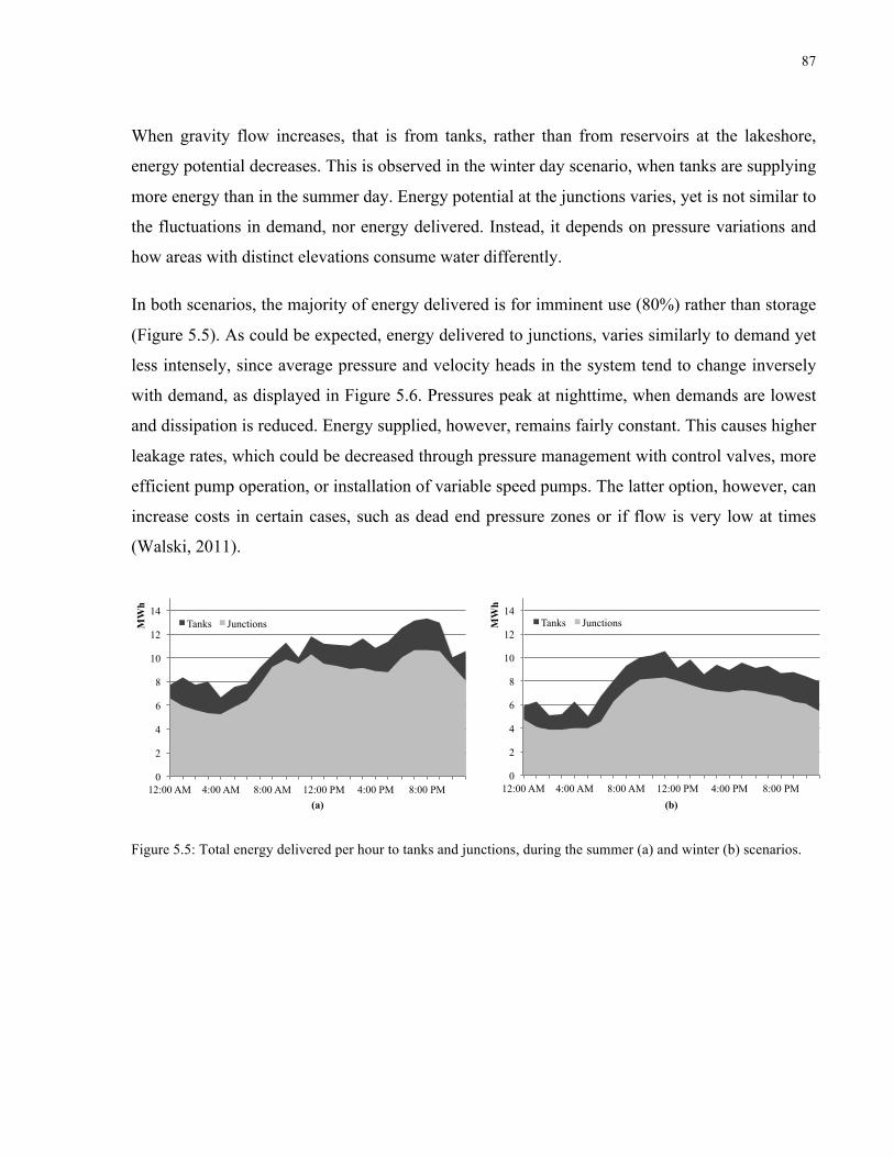
87
When gravity flow increases, that is from tanks, rather than from reservoirs at the lakeshore,
energy potential decreases. This is observed in the winter day scenario, when tanks are supplying
more energy than in the summer day. Energy potential at the junctions varies, yet is not similar to
the fluctuations in demand, nor energy delivered. Instead, it depends on pressure variations and
how areas with distinct elevations consume water differently.
In both scenarios, the majority of energy delivered is for imminent use (80%) rather than storage
(Figure 5.5). As could be expected, energy delivered to junctions, varies similarly to demand yet
less intensely, since average pressure and velocity heads in the system tend to change inversely
with demand, as displayed in Figure 5.6. Pressures peak at nighttime, when demands are lowest
and dissipation is reduced. Energy supplied, however, remains fairly constant. This causes higher
leakage rates, which could be decreased through pressure management with control valves, more
efficient pump operation, or installation of variable speed pumps. The latter option, however, can
increase costs in certain cases, such as dead end pressure zones or if flow is very low at times
(Walski, 2011).
Figure 5.5: Total energy delivered per hour to tanks and junctions, during the summer (a) and winter (b) scenarios.
0
2
4
6
8
10
12
14
12:00 AM 4:00 AM 8:00 AM 12:00 PM 4:00 PM 8:00 PM
MW
h
(a)
Tanks Junctions
0
2
4
6
8
10
12
14
12:00 AM 4:00 AM 8:00 AM 12:00 PM 4:00 PM 8:00 PM
MW
h
(b)
Tanks Junctions

88
Figure 5.6: Average head (pressure and kinetic) and total demand at junctions per hour, during the summer (a) and winter (b) scenarios.
The daily energy costs and greenhouse gas emissions of the given winter scenario are
CD$47,000 and, 116 tCO2 respectively. In the summer scenario, increased demands lead to
greater energy costs, CD$60,000. Emissions, however, are unexpectedly lower, 107 tCO2,
because less energy from coal and natural gas sources is used. Overall, energy use for water
pumping represents around 10% of all energy used and 8% of greenhouse gases emitted by city
facilities in Toronto (City of Toronto, 2014).
Energy costs, and increasingly GHG emissions, are important factors in planning energy use.
These are not necessarily opposing objectives. Electricity tariffs are generally highest during
peak hours, and in Ontario, so are GHG emission factors (Figure 5.7 and Figure 5.8). While
energy generated from renewable sources remains fairly constant throughout the day, fossil fuels
meet the peak demands. If reducing costs is the primary objective, as is generally the case, extra
water should be delivered to tanks at night so that the system can rely more gravity flow during
the day. However for the given scenarios, modeling results show that energy supplied by pumps
varies little compared to the fluctuation in electricity rates. A small reduction in pumping is
observed during peak hours in the summer scenario, but in the winter scenario it even increases
during the day (Figure 5.8).
0
5
10
15
20
25
30
35
45
46
47
48
49
50
51
52
53
54
55
12:00 AM 4:00 AM 8:00 AM 12:00 PM 4:00 PM 8:00 PM
m3.s-1 m
(a)
Average Head
Demand Delivered to Junctions 0
5
10
15
20
25
30
35
45
46
47
48
49
50
51
52
53
54
55
12:00 AM 4:00 AM 8:00 AM 12:00 PM 4:00 PM 8:00 PM
m3.s-1 m
(b)
Average Head
Demand Delivered to Junctions

89
The energy supplied by tanks oscillates throughout the day, especially in the winter scenario,
which also causes energy dissipated in pipes to vary intensely. This occurs because the network
is designed for larger, summer, flows. Therefore, during the winter pumps are cycled more often,
as shown in Figure 5.8, and tanks often alternate between receiving and delivering flows.
Figure 5.7: Energy supplied by tanks and GHG emission factor per hour, during the summer (a) and winter (b) scenarios.
Figure 5.8: Energy supplied by pumps, and water rate per hour, during the summer (a) and winter (b) scenarios.
5.3.1.2 Modified summer scenario
In order for energy supplied by pumps to increase at night and for tanks to supply more of the
peak demand, there must be sufficient pumping and storage capacity. Energy delivered to tanks
would then vary inversely with demand. In the summer scenario, Figure 5.9, this effect is
0
0.05
0.1
0.15
0.2
0.25
0
1
2
3
4
5
6
7
8
9
12:00 AM 4:00 AM 8:00 AM 12:00 PM 4:00 PM 8:00 PM tC
O2.M
Wh-1
MW
h
(a)
Energy Supplied by Tanks
Emission Factor
0
0.05
0.1
0.15
0.2
0.25
0
1
2
3
4
5
6
7
8
9
12:00 AM 4:00 AM 8:00 AM 12:00 PM 4:00 PM 8:00 PM
tCO
2.MW
h-1
MW
h (b)
Energy Supplied by Tanks
Emission Factor
0
2
4
6
8
10
12
0
5
10
15
20
25
30
35
40
12:00 AM 4:00 AM 8:00 AM 12:00 PM 4:00 PM 8:00 PM
cent
s.kW
h-1
MW
h
(a)
Energy Supplied by Pumps
Electricity Rate 0
2
4
6
8
10
12
0
5
10
15
20
25
30
35
40
12:00 AM 4:00 AM 8:00 AM 12:00 PM 4:00 PM 8:00 PM
cent
s.kW
h-1
MW
h
(b)
Energy Supplied by Pumps
Electricity Rate

90
observed at the beginning of the day, but as demand increases in the evening, more energy is
delivered to tanks. In the winter scenario, despite the fluctuations, a trend can be seen as energy
delivered to tanks increases as demands decrease.
Figure 5.9: Demand delivered to junctions and energy delivered to tanks per hour, during the summer (a) and winter (b) scenarios.
Based on the given model scenarios, tank capacity is not the primary constraint to decreasing
energy supplied by pumps during peak electricity hours. Almost half of the pumps are kept on
during the whole day in these scenarios, despite available tank capacity, high electricity costs,
and slightly high pressures in the system. Usual Toronto Water practice is to reduce pumping at
peak times. Additional controls might need to be added to the model so that results better
approximate operator practices.
In order to assess potential improvements, a modified version of the summer scenario was run. In
it, 20% of the open pumps were closed between 11 a.m. and 4 p.m. Energy supplied by pumps
consequently decreases during this period by 5%, as shown in Figure 5.10a, but tanks provide
pressure equalization and daily energy delivered to the junctions is only reduced 1%, (Figure
5.10b). Electricity costs and GHG emissions are reduced by 6%. Over an extended period,
however, even if tanks were maintained at lower levels this temporary reduction in pumping
would be offset by a subsequent increase in order to refill tanks. Therefore, significant changes
could only be made to costs and emissions by altering pump scheduling. Even a 5% reduction to
0
0.5
1
1.5
2
2.5
3
0
5
10
15
20
25
30
35
12:00 AM 4:00 AM 8:00 AM 12:00 PM 4:00 PM 8:00 PM m
3 .s-1
MW
h
(a)
Demand Delivered to Junctions Energy Delivered to Tanks 0
0.5
1
1.5
2
2.5
3
0
5
10
15
20
25
30
35
12:00 AM 4:00 AM 8:00 AM 12:00 PM 4:00 PM 8:00 PM
m3 .s
-1
MW
h
(b)
Demand Delivered to Junctions Energy Delivered to Tanks
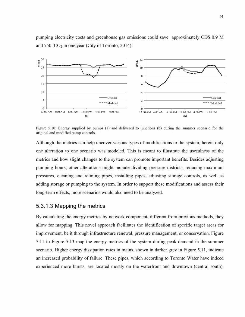
91
pumping electricity costs and greenhouse gas emissions could save approximately CD$ 0.9 M
and 750 tCO2 in one year (City of Toronto, 2014).
Figure 5.10: Energy supplied by pumps (a) and delivered to junctions (b) during the summer scenario for the original and modified pump controls.
Although the metrics can help uncover various types of modifications to the system, herein only
one alteration to one scenario was modeled. This is meant to illustrate the usefulness of the
metrics and how slight changes to the system can promote important benefits. Besides adjusting
pumping hours, other alterations might include dividing pressure districts, reducing maximum
pressures, cleaning and relining pipes, installing pipes, adjusting storage controls, as well as
adding storage or pumping to the system. In order to support these modifications and assess their
long-term effects, more scenarios would also need to be analyzed.
5.3.1.3 Mapping the metrics
By calculating the energy metrics by network component, different from previous methods, they
allow for mapping. This novel approach facilitates the identification of specific target areas for
improvement, be it through infrastructure renewal, pressure management, or conservation. Figure
5.11 to Figure 5.13 map the energy metrics of the system during peak demand in the summer
scenario. Higher energy dissipation rates in mains, shown in darker grey in Figure 5.11, indicate
an increased probability of failure. These pipes, which according to Toronto Water have indeed
experienced more bursts, are located mostly on the waterfront and downtown (central south),
0
5
10
15
20
25
30
12:00 AM 4:00 AM 8:00 AM 12:00 PM 4:00 PM 8:00 PM
MW
h
(a)
Original
Modified
0
2
4
6
8
10
12
12:00 AM 4:00 AM 8:00 AM 12:00 PM 4:00 PM 8:00 PM
MW
h
(b)
Original
Modified

92
where water leaves the treatment plants. These should, thus, be further assessed and more closely
maintained. Pumps that dissipate large amounts of energy are also key objects for refurbishment.
During this period, pumps provide most of energy supplied (Figure 5.12), while tanks
predominantly receive water (Figure 5.13). Highest energy delivery rates to junctions are
observed downtown and in the northwest, prompting inquiries into pressure management and
perhaps conservation. However, further away from the downtown core and the waterfront, there
are fewer branches and delivery points in the system. Therefore, energy delivered could seem
artificially high because of the larger populations supplied.
Figure 5.11: Map of energy dissipated in the Toronto water distribution network during peak demand (8 p.m.) on maximum demand day.

93
Figure 5.12: Map of energy supplied in the Toronto water distribution network during peak demand (8 p.m.) on maximum demand day.
Figure 5.13: Map of energy delivered in the Toronto water distribution network during peak demand (8 p.m.) on maximum demand day.

94
Improvements to the system can also be prioritized according to energy delivered, as areas that
receive more energy generate greater costs. While revenue is generally a function of demand
(water rates in Toronto are based on volumetric consumption) expenses are a more complex
function of multiple variables, creating the potential for ineffective cost allocation. The energy
metrics can be applied in better understanding these expenses. The Electric Power Research
Institute (2002) discusses some of the factors that can influence unit electricity consumption,
such as system age, restrictions, standards, economies of scale, and equipment replacement.
However, the extent of their impact to consumption depends on the system itself. Modeling the
network with hydraulic models can also provide a greater level of detail to decision-making.
Given the results from the energy metrics, identified target areas, and potential solutions,
alternatives can be simulated and compared to the base scenario to confirm they indeed solve the
issue. Future studies can use these metrics to analyze different networks, scenarios, and
alternatives for improvement. The metrics can also be complemented with more detailed data,
such as break and leakage rates, in order to further study correlations.
5.3.1.4 Extensions of the study
The metrics proposed herein have been presented to the Toronto Water staff. Comments and
questions from these meetings inspired many of the previous discussions of the metrics and their
applications. The metrics and the lens of sustainability they add to system analysis invoke
inquiries over concepts that were taken for granted, such as operational paradigms, maintenance
strategies, rate structures, and standards. If expense reduction is the goal, or, more holistically,
sustainability, a decrease in energy consumption is central, as well as the use of more renewable
energy sources. Both objectives are achieved through the reduction of pressure and flow, perhaps
with refurbished pumps, new pipes, more conservation initiatives and revised pressure
requirements.
The present research and findings inspired further applications and studies. The energy costs and
inefficiencies faced by the Toronto network not only motivated investigations into pressure
management, but also a comparative study of international fire flow and residual pressure
standards. These differ by country, as paradigms and practices regarding failure mitigation vary.

95
North American standards are among the most restrictive even though system safety is
maintained with lower flows and pressures in other regions.
While high pressures in the northern part of the network could be addressed through pressure
management, the simultaneous occurrence of high and low pressures in the downtown pressure
district prompted further research into the motivating factors and effects of dividing pressure
districts. Whether by installing pressure reducing valves, decreasing pumping, or dividing
pressure districts, altering pressures, even within current standards, can affect customer
satisfaction, demands, and utility revenue. Accordingly, the potential revenue impacts of pressure
management were investigated as well as example cases of water rate structures that account for
different delivery pressures.
5.4 Conclusions
The present chapter proposes several integrated energy metrics and applies them to a case study
of the Toronto water distribution system. These assess more than electricity consumption.
Energy supplied is an indicator of operational costs as well as greenhouse gas emissions, and can
thus be used to support a business case for reducing network energy use. Energy lost represents
system leakage and the need for pressure management as well as increased maintenance, while
energy dissipated also reveals the need for demand management. Energy delivered shows how
much energy actually reaches the consumer and, accordingly, motivates improvements to zoning,
design standards, as well as reducing pressures and demands.
Calculating the metrics by component disaggregates water distribution systems so that they are
not analyzed as a simple black box with inputs and outputs, and allows for the identification of
areas or specific system components, where changes are most beneficial. This novel approach
enables the mapping of energy metrics, providing a geographical snapshot of the system.
In the Toronto case study, the amount of energy dissipated (37%), used in overcoming pipe and
valve friction, as well as pump inefficiencies, was found to be similar to energy potential (35%),
96
used in overcoming elevation differences. This is in part due to the size of the network and the
low elevation of the reservoirs. Only 28% of energy supplied is delivered to junctions in the form
of pressure and flow. Consequently, users receive even less, and this inefficiency creates an
important environmental and economic impact. In the modeled scenarios, pumping is not
significantly adjusted to take advantage of off peak electricity rates or lower GHG emission
factors, a practice which Toronto Water seeks to follow. This prompted the development of a
modified scenario, in which peak pumping was reduced by 20%, yet energy delivered was not
greatly affected. This was shown to yield a reduction of 6% to electricity costs and GHG
emissions, revealing the potential benefits of this practice. Nevertheless, an extended simulation
would be needed to assess if safe tank levels can still be maintained.
Mapping energy dissipated revealed key mains for retrofitting in the downtown. Energy
delivered is also highest in this area, which means it could benefit from pressure management
and conservation. While the metrics have shown to be useful indicators of energy efficiency,
infrastructure performance, and costs, as verified by Toronto Water, additional data is required to
support decision-making. In future studies, as in the extended research being completed in
Toronto, the analysis of different scenarios and network configurations can inform the revision
of design standards, operational requirements and maintenance scheduling. In addition, by
systematically applying this methodology to a set of different systems, results can be compared
and generalized between municipalities and benchmarks defined.
97
6 Performance Metrics The energy metrics proposed in chapter 5 are indicators of system capacity, efficiency, GHG
emissions, and specific operational and capital costs. The current chapter applies these in
expanding the analysis of the network, and assessing its performance under different operation
conditions. Because these metrics are derived from the variation of energy metrics over different
normal and emergency conditions, they can also be modeled with EPANET and can easily be
applied by utilities. Previous studies have equated water distribution network performance to the
ability to deliver sufficient pressure and flow. The present chapter argues that this performance
also depends on the efficiency of delivering these requirements
The present chapter is based on the manuscript entitled “Performance Index for Water
Distribution Networks Under Multiple Loading Conditions” by Rebecca Dziedzic and Bryan
Karney, submitted to the Journal of Water Resources Planning and Management. It addresses
the issue of assessing the performance of complex systems, and how it depends on network
design, operations, and maintenance.
6.1 Performance of water distribution networks and other complex systems
The performance of water distribution networks is multi-objective and dependent upon complex
interactions between infrastructure components as well as with external conditions. This can be
compared ecosystems, which must balance population requirements against outside pressures.
Indeed, previous authors have found that ecosystems function according to principles that
increase network sustainability, such as resilience and reliability (Biomimicry 3.8 Institute, 2011;
Ho and Ulanowicz, 2005; Katifori et al., 2010).
The classic 1973 study by Holling argues that evolution finds a balance between two related
system characteristics, namely resilience and stability, with resilience being a term coined for
98
ecosystems to indicate a system’s ability to absorb changes of state variables. Thus, resilience is
related to the concept of persistence, while stability indicates the ability of these systems to
return to an equilibrium state after a temporary disturbance. Therefore, a stable system would not
fluctuate greatly, and a resilient system might undergo significant fluctuations. Klein et al.
(2003) note that despite the continuous debate since the seminal work by Holling (1973), a
consensus on how to operationalize this concept has not been reached. For instance, Timmerman
(1981) links resilience to vulnerability and defines the first as the measure of a system’s capacity
to absorb and recover from a hazardous event. Pimm (1984) connects resilience with stability:
resilience is the speed with which a system returns to its original state after a temporary
disturbance. This definition concerns engineering resilience, which considers ecological systems
to exist close to a single stable steady state (Holling, 1996). Ecological resilience, on the other
hand, emphasizes instabilities, which can lead the system to still function but in another state.
Fiering (1982a) introduces several indices to measure the resilience of water resource systems.
These are related to various system attributes including the probability of the system being in an
acceptable state, the probability of failure, the costs of being in each state, as well as expected
time to change states. Each of these represent different properties of the system, all of which
favourably indicate a system’s performance, and all are highly correlated (Fiering 1982b).
Hashimoto et al. (1982) instead developed a single concept for evaluating water supply system
resilience, and two additional concepts, vulnerability, and reliability to assess system
performance. In Hashimoto, resilience is the probability of recovery from failure within a
specified time interval. As applied to water supply, this is calculated as the probability of quickly
meeting demand after an instance of insufficient supply (Hashimoto et al., 1982; Moy et al.,
1986; Solis et al., 2011). Reliability is the probability of water supply meeting demand during the
period of the simulation (Klemes et al. 1981; Hashimoto et al., 1982; Moy et al., 1986;
McMahon, 2006; Solis et al., 2011). Vulnerability, introduces another consideration, being a
measure of the significance (or consequences) of failure (Hashimoto et al., 1982). This is often
calculated as direct surrogate of costs, such as the average demand deficit during failure events

99
(Loucks and van Beek, 2005; Solis et al., 2011) or the largest deficit during the period of
operation (Moy et al., 1986).
For the analysis of water distribution networks, resilience has largely acquired another meaning,
more related in earlier work to the concept of robustness. Todini (2000) defined water
distribution resilience as the ability of the network to provide more power than required at each
noted in order to have a sufficient surplus to be dissipated internally in case of failure. This
resilience index (6.1) is applied as a surrogate measure of network reliability.
RI =qj (ha j − hrj )
j=1
n∑
QrHr + Pbb=1
B∑
r=1
R∑#
$%
&
'(− qjhrj
j=1
n∑
(6.1)
where n is the number of demand nodes, qj the demand at node j, haj head available at node j, hrj
minimum head required to meet constraints at node j; R the number of reservoirs, Qr the flow
being supplied to the system by reservoir r, Hr the head at reservoir r, Pb the power introduced
in the system by pump b into the system.
Todini’s resilience index has been widely adapted and applied to water distribution system
studies (Todini, 2000; Prasad and Park, 2004; Jayaram and Srinivasam, 2008; Baños, 2011;
Atkinson, 2014; di Nardo, 2014). Prasad and Park (2004) combine the resilience index with a
diameter uniformity coefficient (6.2) in order to better represent the reliability of loops. The
resulting network resilience index NRI is given in (6.3).
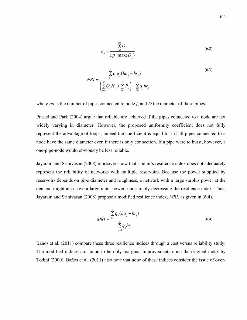
100
c j =Dj
i=1
np∑
np ⋅max(Dj ) (6.2)
NRI =c jq j (ha j − hrj )
j=1
n∑
QrHr + Pbb=1
B∑
r=1
R∑#
$%
&
'(− qjhrj
j=1
n∑
(6.3)
where np is the number of pipes connected to node j, and D the diameter of these pipes.
Prasad and Park (2004) argue that reliable are achieved if the pipes connected to a node are not
widely varying in diameter. However, the proposed uniformity coefficient does not fully
represent the advantage of loops; indeed the coefficient is equal to 1 if all pipes connected to a
node have the same diameter even if there is only connection. If a pipe were to burst, however, a
one-pipe-node would obviously be less reliable.
Jayaram and Srinivasan (2008) moreover show that Todini’s resilience index does not adequately
represent the reliability of networks with multiple reservoirs. Because the power supplied by
reservoirs depends on pipe diameter and roughness, a network with a large surplus power at the
demand might also have a large input power, undesirably decreasing the resilience index. Thus,
Jayaram and Srinivasan (2008) propose a modified resilience index, MRI, as given in (6.4).
MRI =qj (ha j − hrj )
j=1
n∑
qjhrjj=1
n∑
(6.4)
Baños et al. (2011) compare these three resilience indices through a cost versus reliability study.
The modified indices are found to be only marginal improvements upon the original index by
Todini (2000). Baños et al. (2011) also note that none of these indices consider the issue of over-

101
demand is applied, and thus do not accurately determine the capability of the network to deliver
demand under uncertainty.
While these indices do not fully consider the connectivity of a network, and cannot identify
critical areas in the system, Yazdani et al. (2011) focus on non-hydraulic statistical and structural
metrics for assessing water distribution network resilience. The connectivity pattern between
nodes and links is used to calculate reliability, efficiency and robustness of the networks.
Tanyimboh and Templeman (1999) also evaluate network performance according to non-
hydraulic metrics. The authors introduce the concept of entropy in water networks, entropy being
defined as the probability of a node receiving demands given the availability of adequate
alternate flow paths.
Creaco et al. (2014) compare the resilience and entropy metrics as indirect measures of network
reliability. The demand satisfaction rate is assumed to be a natural performance indicator, and a
direct measure of reliability; it is calculated as the ratio of demand delivered to demand required,
based on a pressure driven simulation. The maximum reliability is reached by just meeting the
minimum pressure required to satisfy demands. Pressures above this level do not alter the
assessment of reliability of the network. Given this definition, the resilience indices showed a
much stronger positive correlation with network reliability. Zhuang et al. (2013) and Di Nardo et
al. (2014), in fact, apply the demand satisfaction rate directly to support the assessment of water
distribution networks.
Even the demand satisfaction rate, although dependent upon pressure as well, clearly does not
fully represent the performance of water networks. Delivering pressures above the minimum
requirement to meet full demands does not affect this rate, but does alter both costs and how the
network operates. The resilience metrics account for all pressures, but are partial to higher
network pressures, which despite inducing the supply of surplus power might well lead to higher
leakage and burst rates. The present paper argues that the performance of the network should
depend not only on the ability to deliver adequate flows and pressures, but also on its efficiency
in doing so.

102
As argued when introducing previous resilience indices, power is attractive measure in assessing
networks since it is proportional to pressure and flow, the main products of the system. Cabrera
et al. (2010) propose energy indicators to evaluate the efficiency of networks, defined according
to ratios between energy supplied, energy lost, and useful energy or minimum required useful
energy. These are calculated at a system level for a long-term period in order to represent its
energy balance. Chapter 5 proposes water distribution system energy metrics that are computed
for each component at each time step. This facilitates both the identification of areas for
improvement and the comparison of operational efficiency in different scenarios.
The current study proposes efficiency-based performance metrics for evaluating and comparing
water distribution networks. These metrics accommodate varying loads and multiple network
components in order to represent network connectivity, capacity to deliver demand under
uncertainty, and ability to recover after emergencies. The metrics are applied to two example
networks and variations of these, enabling and provisionally validating their use in as network
assessment tools.
6.2 Performance Index
Four metrics are herein defined for evaluating water network performance: reliability, resilience,
vulnerability, and connectivity. The first three are conceptually based on definitions used in
water basin management, as described in the previous section (Klemes et al. 1981; Hashimoto et
al., 1982; Moy et al., 1986; Loucks and van Beek, 2005; McMahon, 2006; Solis et al., 2011).
Because the performance of water networks depends on the efficient delivery of sufficient
demand and pressure, energy efficiency is applied instead of demand to compute the metrics.
Furthermore, unlike in water basin studies where a minimum demand is established, or the
network resilience indices where a minimum pressure is determined, a minimum efficiency
constraint has not been established. Accordingly, the proposed metrics do not evaluate the
probability of the network meeting a minimum efficiency, but rather the efficiency of the
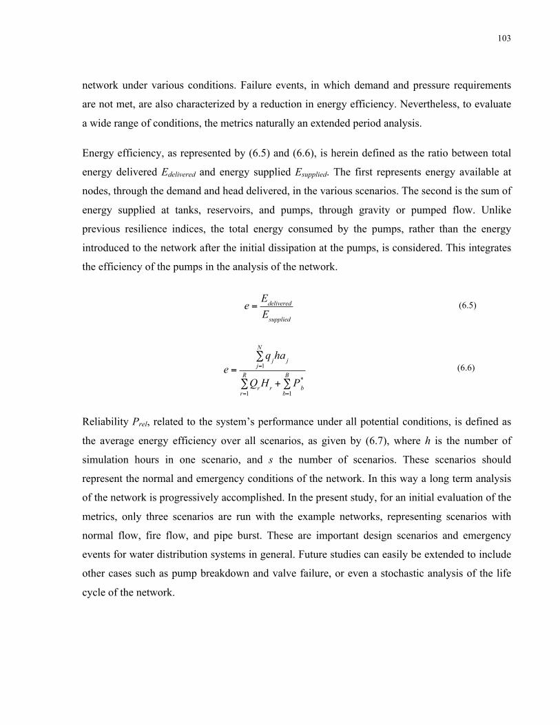
103
network under various conditions. Failure events, in which demand and pressure requirements
are not met, are also characterized by a reduction in energy efficiency. Nevertheless, to evaluate
a wide range of conditions, the metrics naturally an extended period analysis.
Energy efficiency, as represented by (6.5) and (6.6), is herein defined as the ratio between total
energy delivered Edelivered and energy supplied Esupplied. The first represents energy available at
nodes, through the demand and head delivered, in the various scenarios. The second is the sum of
energy supplied at tanks, reservoirs, and pumps, through gravity or pumped flow. Unlike
previous resilience indices, the total energy consumed by the pumps, rather than the energy
introduced to the network after the initial dissipation at the pumps, is considered. This integrates
the efficiency of the pumps in the analysis of the network.
e = EdeliveredEsupplied
(6.5)
e =qjha j
j=1
N∑
QrHr + P*bb=1
B∑
r=1
R∑
(6.6)
Reliability Prel, related to the system’s performance under all potential conditions, is defined as
the average energy efficiency over all scenarios, as given by (6.7), where h is the number of
simulation hours in one scenario, and s the number of scenarios. These scenarios should
represent the normal and emergency conditions of the network. In this way a long term analysis
of the network is progressively accomplished. In the present study, for an initial evaluation of the
metrics, only three scenarios are run with the example networks, representing scenarios with
normal flow, fire flow, and pipe burst. These are important design scenarios and emergency
events for water distribution systems in general. Future studies can easily be extended to include
other cases such as pump breakdown and valve failure, or even a stochastic analysis of the life
cycle of the network.
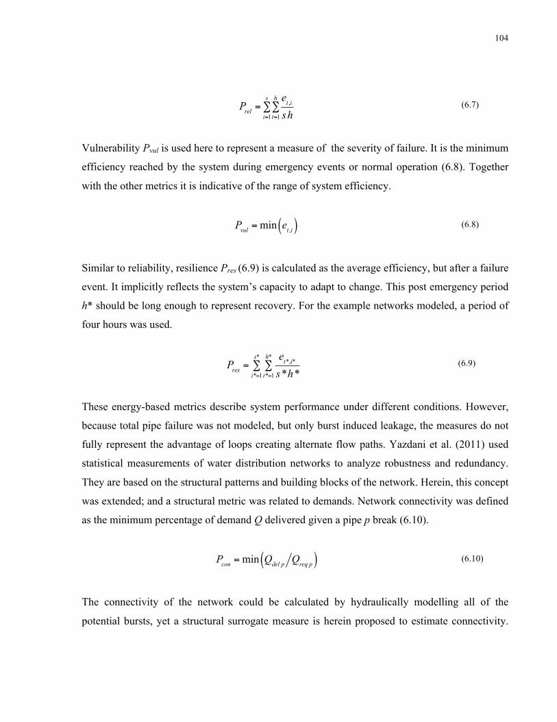
104
Prel =et ,isht=1
h∑
i=1
s∑ (6.7)
Vulnerability Pvul is used here to represent a measure of the severity of failure. It is the minimum
efficiency reached by the system during emergency events or normal operation (6.8). Together
with the other metrics it is indicative of the range of system efficiency.
(6.8)
Similar to reliability, resilience Pres (6.9) is calculated as the average efficiency, but after a failure
event. It implicitly reflects the system’s capacity to adapt to change. This post emergency period
h* should be long enough to represent recovery. For the example networks modeled, a period of
four hours was used.
Pres =et*,i*s*h*t*=1
h*∑
i*=1
s*∑ (6.9)
These energy-based metrics describe system performance under different conditions. However,
because total pipe failure was not modeled, but only burst induced leakage, the measures do not
fully represent the advantage of loops creating alternate flow paths. Yazdani et al. (2011) used
statistical measurements of water distribution networks to analyze robustness and redundancy.
They are based on the structural patterns and building blocks of the network. Herein, this concept
was extended; and a structural metric was related to demands. Network connectivity was defined
as the minimum percentage of demand Q delivered given a pipe p break (6.10).
Pcon =min Qdel p Qreq p( ) (6.10)
The connectivity of the network could be calculated by hydraulically modelling all of the
potential bursts, yet a structural surrogate measure is herein proposed to estimate connectivity.
Pvul =min et ,i( )

105
The connectivity vector, given in (6.11), indicates if nodes are connected to a source of water.
The network is represented as an adjacency matrix, A, of order n x n, where n is the number of
nodes. The elements of the matrix represent the network connections. As usual, lines and
columns indicate specific nodes with values of 1 indicating that a pipe directly connects the
respective nodes, and 0 otherwise. The location of the sources is represented in a vector, c0,
where elements are either 1 if the node is a source or 0 if not. The elements of the resulting
connectivity vector, c, are 0 if the particular node is not connected to any source of water, and
different from 0 if it is.
c = c0j=1
n∑ Aj (6.11)
For the purposes of this study, the demand-based connectivity, (6.10), was thus estimated
assuming that a network connection between a source of water and a node would suffice for
water to be delivered.
In order to evaluate these collectively, an aggregate performance index is proposed. As shown in
(6.12), this aggregate measure is taken as the geometric average of the performance metrics (Pm):
reliability, resilience, vulnerability, and connectivity. Because these are ratios of either” energy
delivered to supplied” or “demand delivered to required”, they all range between 0 and 1. The
upper limit indicates the best situation. Other properties of this type of index are attractive: (1) if
one of the metrics is zero, the index will be zero; (2) if the metrics are all equal, so is the overall
measure; (3) there is an implicit weighting, through which the “worst” metrics are given more
importance; and (4) each metric is considered essential and irreplaceable. In accordance with the
second property, results from a geometric average are similar to those from an arithmetic average
if efficiencies are consistent. However, for systems with a wider range of performance, because
the worst metrics are given more importance, the geometric average represents this inconsistency
better.

106
(6.12)
6.3 Case Studies
In order to assess the performance and usefulness of the metrics, two example networks are
assessed, with each having a range of pipe redundancy increasing strategies, as well as pumping
and storage scenarios. Increasing network redundancy, whether through adding pipes or other
components, is a recognized strategy for increasing network performance, especially resilience
(Awumah et al., 1990; Goulter, 2004; Walski, 2004; National Research Council, 2006; U.S.
Department of the Interior Bureau of Reclamation, 2006; Yazdani et al, 2011). The proposed
metrics were also compared to the resilience indices developed by Todini (2000), Prasad and
Park (2004), and Jayaram and Srinivasam (2008), as well as the average pressure of the network.
The two example networks modeled are based on examples distributed with EPANET (2000).
They were selected because both are not only well known but have at least one reservoir, tank,
and pump, as well as hourly varying demands. This allows for the analysis of storage and
multiple loading conditions not evaluated by other authors (Todini, 2000; Baños, 2011;
Atkinson, 2014). The demand patterns were altered to better represent urban demand, with two
peaks, in the morning and the evening (Blokker et al., 2010). Demand, however, was set to
fluctuate more than would be expected during normal operations, varying between minimum (0
h), average (3 h), maximum (6 h), and peak demand (17 h) throughout the day, shown in Figure
6.1. Peaking coefficients were based on recommendations from Municipal Engineers Association
(1977) and Ysusi (1999). This not only enables the analysis of different extreme scenarios, but
also of system response to wide variations in demand. Further network modifications were made
in order to maintain normal operations within standard pressure ranges. Pressure ranges were
verified for the original looped configurations of the networks. However, in other configurations,
PI = Pmm=1
M
∏"
#$
%
&'
1M
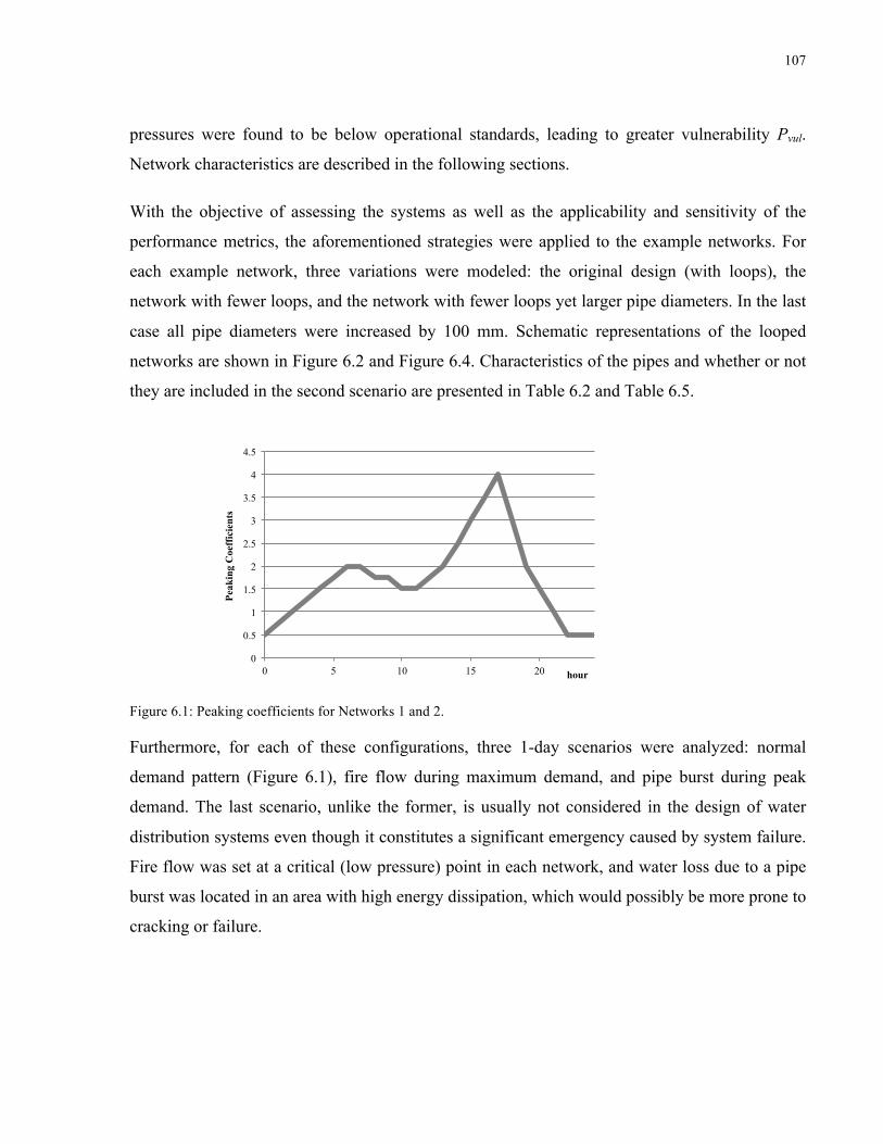
107
pressures were found to be below operational standards, leading to greater vulnerability Pvul.
Network characteristics are described in the following sections.
With the objective of assessing the systems as well as the applicability and sensitivity of the
performance metrics, the aforementioned strategies were applied to the example networks. For
each example network, three variations were modeled: the original design (with loops), the
network with fewer loops, and the network with fewer loops yet larger pipe diameters. In the last
case all pipe diameters were increased by 100 mm. Schematic representations of the looped
networks are shown in Figure 6.2 and Figure 6.4. Characteristics of the pipes and whether or not
they are included in the second scenario are presented in Table 6.2 and Table 6.5.
Figure 6.1: Peaking coefficients for Networks 1 and 2.
Furthermore, for each of these configurations, three 1-day scenarios were analyzed: normal
demand pattern (Figure 6.1), fire flow during maximum demand, and pipe burst during peak
demand. The last scenario, unlike the former, is usually not considered in the design of water
distribution systems even though it constitutes a significant emergency caused by system failure.
Fire flow was set at a critical (low pressure) point in each network, and water loss due to a pipe
burst was located in an area with high energy dissipation, which would possibly be more prone to
cracking or failure.
0
0.5
1
1.5
2
2.5
3
3.5
4
4.5
0 5 10 15 20
Peak
ing
Coe
ffic
ient
s
hour

108
The additional demands due to fire and leakage, each with a duration of 2 hours, were assigned
to dummy nodes, connected to the network by short pipes with insignificant head loss. The fire
flow was determined based on the demands in the system and the ISO (2008) recommendations
for residential dwellings. In Network 1, the fire flow is 63 L.s-1, and in Network 2, 126 L.s-1.
Lambert et al. (2000) compared seven North American water distribution systems. Their leakage
rates represented between 15 and 33% of total system input volume. In the present models, the
leakage in the pipe burst scenario was set to 20% of total demand. Although this is clearly a
significant flow at a single node, it is less than many consistent leakage rates, and allows for the
assessment of critical leakage on network performance. Leaks were defined as emitters in
EPANET, with a pressure exponent of 1, as suggested by Lambert (2000). This resulted in a
discharge coefficient of 0.7 for Network 1 and 2.9 for Network 2.
6.3.1 Example Network 1
Network 1 is a simple 3 loop-network, shown in Figure 6.2. It has one reservoir and one tank,
both at higher elevations than the remaining nodes. The initial level of the tank is 36 m, while the
minimum and maximum level are 31 m and 46 m, respectively. Although gravity flow does play
a role in supplying flow, pumping is still required. The pump curve is defined by one head vs.
flow coordinate, 76.2 m for 94.6 L.s-1.
Three network configurations were modelled: the original (looped) system, the same system with
fewer loops, and with increased diameters. The basic node characteristics are the same for all
three and are given in Table 6.1. Pipe characteristics of the looped network are listed in Table
6.2. In the second configuration, three pipes were removed, indicated by an asterisk in Table 6.2,
and all other characteristics were maintained. In the third configuration, the same pipes are
removed yet all other diameters are increased by 100 mm.
The average pumping energy varies minimally between the three modeled configurations of
Network 1, original (looped), fewer loops, and increased diameters, as shown in Table 6.3.
Therefore, operational energy costs are stable despite structural differences. The energy
dissipated however, varies significantly. The configuration with fewer loops consistently

109
presents lower pressures and energy efficiency. Consumers would be receiving an inferior
service in this case, and utilities would be spending more money on overcoming friction. Risks
associated with pipe breaks or low pressures would also be higher.
Table 6.1: Elevation and demand values for Network 1 nodes.
Node ID Elev (m) Q (L.s-1) Res 243.8
Tank 259.1 10 216.4 0.0
11 216.4 9.5 12 213.4 9.5 13 211.8 6.3 21 213.4 9.5 22 211.8 12.6 23 210.3 9.5 31 213.4 6.3 32 21.6 6.3
Figure 6.2: Schematic representation of Network 1with node IDs. Table 6.2: Length, diameter, and roughness coefficient values for Network 1 pipes.

110
Pipe ID Start Node End Node L (m) D (mm) C 10 10 11 3209.5 457.2 100 11 11 12 1609.3 355.6 100 12 12 13 1609.3 254.0 100
21* 21 22 1609.3 254.0 100 22 22 23 1609.3 304.8 100 31 31 32 1609.3 152.4 100
110 Tank 12 61.0 457.2 100 111 11 21 1609.3 254.0 100
112* 12 22 1609.3 304.8 100 113 13 23 1609.3 203.2 100 121 21 31 1609.3 203.2 100
122* 22 32 1609.3 152.4 100 * Pipes not included in the configuration with fewer loops
Table 6.3: Average energy metrics of the alternative configurations of Network 1, L – fewer loops, D – larger diameters.
Network Pump Esupplied (kWh) Edissipated + Elost (kWh)
Net 1 91.4 25.7
Net 1 L 91.4 36.8
Net 1 L, D 91.4 26.7
The daily energy efficiency profiles of the alternative configurations of Network 1 are shown in
Figure 6.3. The percentage of energy delivered, equivalent to e, in the original looped
configuration of Network 1 varies between 80 and 84%. The additional demands during peak
hours as well as during fire events increase system efficiency (Figure 6.3a). Despite the increased
energy dissipation in the pipes due to larger flows, tanks supply more water during this period.
This allows pumps to operate at the same level, at similar dissipation rates as during normal
operations, momentarily increasing efficiency. Obviously this efficiency cannot be sustained but
shows how storage can be used to maintain the reliability of the system. This is also true in the
configuration with increased diameters (Figure 6.3c), but not in the case with fewer loops (Figure
6.3b). In the latter, the additional flow during fire events and peak hours causes excessive pipe
dissipation, reducing energy efficiency. In all three cases, then the burst occurs during peak flow,
the energy lost through leakage causes efficiency to plummet.

111
Figure 6.3: Energy efficiency profile over 24-hour simulation for Network 1 (a) original network, (b) fewer loops, (c) larger diameters.
(a)
(b)
(c)
50%
55%
60%
65%
70%
75%
80%
85%
90%
95%
0 5 10 15 20 hour
Normal
Fire
Burst
50%
55%
60%
65%
70%
75%
80%
85%
90%
95%
0 5 10 15 20 hour
Normal
Fire
Burst
50%
55%
60%
65%
70%
75%
80%
85%
90%
0 5 10 15 20 hour
Normal
Fire
Burst

112
Table 6.4: Proposed performance metrics, resilience index (Todini, 2000), network resilience index (Prasad and Park, 2004), modified resilience index (Jayaram and Srinivasam, 2008), and average pressure of the alternative configurations of Network 1, L – fewer loops, D – larger diameters.
Network Rel Vul Res Con PI RI NRI MRI Avg P Net 1 0.84 0.80 0.83 1.00 0.86 0.99 0.80 1.15 83.94 Net 1 L 0.77 0.54 0.79 0.59 0.66 0.87 0.76 0.97 78.60 Net 1 L, D 0.83 0.71 0.82 0.59 0.73 0.97 0.87 1.12 83.14
These differences are clear in the performance metrics shown in Table 6.4. While reliability and
resilience are similar for the configurations with greater redundancy, they are lower in the
configuration with fewer loops. The greater connectivity and lower vulnerability in the looped
network lead to a higher performance index, setting it apart from the configuration with larger
diameters.
The proposed performance index follows the same trend as the resilience index by Todini (2000)
and the modified resilience index by Jayaram and Srinivasam (2008). All indicate that the looped
configuration has the best performance. Nevertheless, the difference between the looped and the
larger diameter configuration is small according to the resilience indices. Because these are
proportional to the power surplus they vary similarly to the average pressure of the networks.
The inclusion of vulnerability and connectivity into the proposed performance index helps to
distinguish the real performance differences of the networks.
The index defined by Prasad and Park (2004) is the only metric that is more partial to the
configuration with no loops and larger diameters. Removing pipes or increasing diameters has a
greater effect on node uniformity in smaller networks, such as the given example. Thus, an
advantage is given to branched networks with more nodes reached only by a single pipe.
6.3.2 Example Network 2
Network 2 is more complex and better represents many systems. It has two reservoirs, three
tanks, and two pumps, shown in Figure 6.4. In this case, nine configurations were modelled in
order to assess modifications to storage and pumping, as well pipe redundancy. Three storage
and pumping configurations were evaluated: the original, a scenario with reduced storage, and
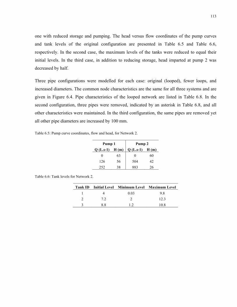
113
one with reduced storage and pumping. The head versus flow coordinates of the pump curves
and tank levels of the original configuration are presented in Table 6.5 and Table 6.6,
respectively. In the second case, the maximum levels of the tanks were reduced to equal their
initial levels. In the third case, in addition to reducing storage, head imparted at pump 2 was
decreased by half.
Three pipe configurations were modelled for each case: original (looped), fewer loops, and
increased diameters. The common node characteristics are the same for all three systems and are
given in Figure 6.4. Pipe characteristics of the looped network are listed in Table 6.8. In the
second configuration, three pipes were removed, indicated by an asterisk in Table 6.8, and all
other characteristics were maintained. In the third configuration, the same pipes are removed yet
all other pipe diameters are increased by 100 mm.
Table 6.5: Pump curve coordinates, flow and head, for Network 2.
Pump 1 Pump 2 Q (L.s-1) H (m) Q (L.s-1) H (m)
0 63 0 60 126 56 504 42 252 38 883 26
Table 6.6: Tank levels for Network 2.
Tank ID Initial Level Minimum Level Maximum Level 1 4 0.03 9.8 2 7.2 2 12.3 3 8.8 1.2 10.8

114
Figure 6.4: Schematic representation of Network 2 with node IDs.

115
Table 6.7: Elevation and demand values for Network 2 nodes.
Node ID Elev (m) Q (L.s-1) Node ID Elev (m) Q (L.s-1) Node ID Elev (m) Q (L.s-1) Res1 50.9
143 -1.4 0.4 206 0.3 0.0
Res2 67.1
145 0.3 1.7 207 2.7 4.4 Tank1 39.3
147 5.6 0.5 208 4.9 0.0
Tank2 40.2
149 4.9 1.7 209 -0.6 0.1 Tank3 35.5
151 10.2 9.1 211 2.1 0.5
10 44.8 0.0 153 20.2 2.8 213 2.1 0.9 15 9.8 0.1 157 4.0 3.3 215 2.1 5.8 20 39.3 0.0 159 1.8 2.6 217 1.8 1.5 35 3.8 0.1 161 1.2 1.0 219 1.2 2.6 40 40.2 0.0 163 1.5 0.6 225 2.4 1.4 50 35.5 0.0 164 1.5 0.0 229 3.2 4.0 60 0.0 0.0 166 -0.6 0.2 231 1.5 1.0
601 0.0 0.0 167 -1.5 0.9 237 4.3 1.0 61 0.0 0.0 169 -1.5 0.0 239 4.0 2.8
101 12.8 12.0 171 -1.2 2.5 241 4.0 0.0 103 13.1 8.4 173 -1.2 0.0 243 4.3 0.3 105 8.7 8.5 177 2.4 3.7 247 5.5 4.4 107 6.7 3.4 179 2.4 0.0 249 5.5 0.0 109 6.2 14.6 181 2.4 0.0 251 9.1 1.5 111 3.0 9.0 183 3.4 0.0 253 11.0 3.4 113 0.6 1.3 184 4.9 0.0 255 8.2 2.5 115 4.3 3.3 185 4.9 1.6 257 5.2 0.0 117 4.1 7.4 187 3.8 0.0 259 7.6 0.0 119 0.6 11.1 189 1.2 6.8 261 0.0 0.0 120 0.0 0.0 191 7.6 5.2 263 0.0 0.0 121 -0.6 2.6 193 5.5 4.5 265 0.0 0.0 123 3.4 0.1 195 4.7 0.0 267 6.4 0.0 125 3.4 2.9 197 7.0 1.1 269 0.0 0.0 127 17.1 1.1 199 -0.6 7.5 271 1.8 0.0 129 15.5 0.0 201 0.0 2.8 273 2.4 0.0 131 1.8 2.7 203 0.6 0.1 275 3.0 0.0 139 9.4 0.4 204 6.4 0.0
141 1.2 0.6 205 6.4 4.1

116
Table 6.8: Length, diameter, and roughness coefficient values for Network 2 pipes.
Pipe ID
Start Node
End Node L (m)
D (mm) C
Pipe ID
Start Node
End Node L (m)
D (mm) C
Pipe ID
Start Node
End Node L (m)
D (mm) C
20 Tank1 20 30 2515 199 175 157 159 887 762 141 243 209 211 369 406 130 40 Tank2 40 30 2515 199 177 159 161 610 762 141 245 211 213 302 406 130 50 Tank3 50 30 2515 199 179 161 163 131 762 141 247 213 215 1306 406 130 60 Res 2 60 375 610 140 180 163 164 46 356 130 249 215 217 506 406 130 101 10 101 4328 457 110 181 164 166 149 356 130 251 217 219 625 356 130 103 101 103 411 406 130 183 265 169 180 762 141 257 217 225 475 305 130 105 101 105 774 305 130 185 167 169 18 203 130 261* 213 229 671 203 130 107 105 107 448 305 130 186 187 204 30 203 130 263 229 231 597 305 130 109 103 109 1201 406 130 187 169 171 387 762 141 269 211 237 634 305 130 111 109 111 610 305 130 189 171 173 15 762 141 271 237 229 241 203 130 112* 115 111 354 305 130 191 271 171 232 610 130 273 237 239 155 305 130 113* 111 113 512 305 130 193 35 181 9 610 130 275 239 241 11 305 130 114 115 113 610 203 130 195 181 177 9 305 130 277 241 243 671 305 130 115 107 115 594 203 130 197 177 179 9 305 130 281* 241 247 136 254 130 116 113 193 506 305 130 199 179 183 64 305 130 283 239 249 131 305 130 117 263 105 831 305 130 201 40 179 363 305 130 285 247 249 3 305 130 119* 115 117 664 305 130 202 185 184 30 203 130 287 247 255 424 254 130 120 119 120 223 305 130 203 183 185 155 203 130 289 50 255 282 254 130 121* 120 117 570 305 130 204 184 205 1381 305 130 291 255 253 335 254 130 122* 121 120 625 203 130 205 204 185 404 305 130 293* 255 251 335 203 130 123 121 119 610 762 141 207 189 183 411 305 130 295 249 251 442 305 130 125 123 121 457 762 141 209* 189 187 152 203 130 297 120 257 197 203 130 129 121 125 283 610 130 211 169 269 197 305 130 299 257 259 107 203 130 131 125 127 988 610 130 213 191 187 780 305 130 301 259 263 427 203 130

117
Table 6.8 (cont.): Length, diameter, and roughness coefficient values for Network 2 pipes.
Pipe ID
Start Node
End Node L (m)
D (mm) C
Pipe ID
Start Node
End Node L (m)
D (mm) C
Pipe ID
Start Node
End Node L (m)
D (mm) C
133 20 127 239 508 130 215 267 189 375 305 130 303* 257 261 427 203 130 135 127 129 274 610 130 217* 191 193 158 305 130 305 117 261 197 305 130 137 129 131 1975 406 130 219 193 195 110 305 130 307 261 263 107 305 130 145 129 139 838 203 130 221* 161 195 701 203 130 309* 265 267 482 203 130 147 139 141 625 203 130 223 197 191 351 305 130 311 193 267 357 305 130 149 143 141 427 203 130 225 111 197 850 305 130 313* 269 189 197 305 130 151 15 143 503 203 130 229 173 199 1219 610 141 315 181 271 88 610 130 153* 145 141 1070 305 130 231 199 201 192 610 141 317* 273 275 680 203 130 155 147 145 671 305 130 233 201 203 37 610 130 319 273 205 197 305 130 159 147 149 268 305 130 235* 199 273 221 305 130 321 163 265 366 762 141 161 149 151 311 203 130 237 205 207 366 305 130 323 201 275 91 305 130 163 151 153 357 305 130 238 207 206 137 305 130 325* 269 271 393 203 130 169* 125 153 1390 203 130 239 275 207 436 305 130 329 61 123 13868 762 140 171 119 151 1055 305 130 240 206 208 155 305 130 330 60 601 0 762 140 173 119 157 634 762 141 241 208 209 270 305 130 333 601 61 0 762 140
* Pipes not included in the configuration with fewer loops

118
Although energy supplied by pumps in the original Network 2 configuration (Table 6.9) is not
much different from that in Network 1, energy dissipated is about four to five times higher in the
former. This low efficiency is largely due to the high percentage of energy dissipated in the pipe
leaving pump 2, which conveys most of the flow when reservoirs are supplying water. The
original Network 2 experiences a wide variation in energy dissipated and consequently in energy
efficiency e, which increases throughout the day from 45 to 70% (Figure 6.5a). These represent
extremes of operation, with large flows in the pipes due to tank filling at the beginning of the
simulation, and small flows at the end. The higher efficiency could, thus, not be sustained and
this 24 hour period does not represent a full cycle of operation.
Table 6.9: Average energy metrics of the alternative configurations of Network 2, L – fewer loops, D – larger diameters, S – reduced storage, P – reduced pumping.
Network Pump Esupplied (kWh) Edissipated + Elost (kWh) Net 2 96.0 135.1 Net 2 L 95.7 142.0 Net 2 L,D 77.3 99.6 Net 2 S 207.2 115.6 Net 2 S,L 208.1 125.1 Net 2 S,L,D 204.6 88.4 Net 2 S,P 135.4 96.6 Net 2 S,P,L 135.7 106.5 Net 2 S,P,L,D 135.0 70.5
During the initial hours of the original Network 2 simulation, both tanks are being filled at a rate
that is more than seven times greater than the total demand at junctions. However, less than 10%
of the water stored is used during peak flow. Therefore, the rate of tank filling is inconsistent
with the rate of draining, generating unnecessarily high flows and head loss. The effects of
oversizing tanks go beyond water quality if they are not operated adequately. Tanks are generally
filled when electricity prices are lowest, at night, which coincides with low water demand.
Nonetheless, the rate at which they are filled must be carefully considered as indicated by the
low energy efficiency of Network 2. The principal purpose of tanks is to provide pressure
equalization, allowing the system to operate closer to a steady state. If tank demand is
unnecessarily high this is not achieved.

119
Figure 6.5: Energy efficiency profile over 24-hour simulation for Network 2 (a) original network, (b) reduced storage, (c) reduced storage and pumping.
(a)
(b)
(c)
10%
20%
30%
40%
50%
60%
70%
80%
90%
100%
0 5 10 15 20 hour
Normal
Fire
Burst
10%
20%
30%
40%
50%
60%
70%
80%
90%
100%
0 5 10 15 20 hour
Normal
Fire
Burst
10%
20%
30%
40%
50%
60%
70%
80%
90%
100%
0 5 10 15 20 hour
Normal
Fire
Burst

120
Because of its high localized head loss in this case, the configuration with larger diameters
produced the highest energy efficiency, as shown in Table 6.10. Accordingly, all of the
performance metrics, except for connectivity are also higher in this configuration. Because
connectivity is only marginally reduced by decreasing the number of loops, this is the best
performing configuration according to the proposed performance index.
Table 6.10: Proposed performance metrics, resilience index (Todini, 2000), network resilience index (Prasad and Park, 2004), modified resilience index (Jayaram and Srinivasam, 2008), and average pressure of the alternative configurations of Network 2, L – fewer loops, D – larger diameters, S – reduced storage, P – reduced pumping.
Network Rel Vul Res Con PI RI NRI MRI Avg P Net 2 0.70 0.45 0.66 0.94 0.66 0.45 0.41 0.48 52.38 Net 2 L 0.68 0.45 0.66 0.92 0.66 0.39 0.37 0.44 51.77 Net 2 L,D 0.77 0.50 0.72 0.92 0.71 0.62 0.59 0.66 55.79 Net 2 S 0.78 0.36 0.80 0.94 0.68 0.85 0.77 1.90 99.34 Net 2 S,L 0.77 0.28 0.80 0.92 0.63 0.82 0.77 1.86 98.53 Net 2 S,L,D 0.82 0.45 0.85 0.92 0.73 0.92 0.87 2.04 104.28 Net 2 S,P 0.78 0.41 0.78 0.94 0.69 0.79 0.72 1.32 78.10 Net 2 S,P,L 0.76 0.34 0.78 0.92 0.66 0.74 0.70 1.26 77.01 Net 2 S,P,L,D 0.83 0.45 0.86 0.92 0.74 0.88 0.84 1.45 82.96
Given the failure of this case of Network 2 to maintain stable efficiencies, further modifications
were made to the system in order to improve its performance and investigate the effects of tank
and pump sizing on system operation. These are the reduced storage, and reduced storage and
pumping cases, described before.
Reducing storage in Network 2 resulted in a more stable operation under normal conditions since
less flow is being directed to tanks and dissipation is reduced. Nevertheless vulnerability
increased, as there is less storage to meet the extra demands during peak hours. Overall, the
average efficiency, 78% is higher than in the original case with more storage, 70%. The energy
supplied by pumps increased more than two-fold (Table 6.9), yet the first case uses more tank
supply and is not representative of a full cycle of operation. Pressures are also higher in the
second case, yet less energy is dissipated.
Simply reducing storage increased energy requirements as less storage is available to meet
demands. Furthermore, pressures almost doubled as pumps were now oversized for the given

121
flow. Therefore, a third variation of the system, with reduced pumping capacity as well as reduce
storage, was modeled. This significantly reduced pumping requirements and average network
pressures, yet did not affect the reliability of the network (Table 6.10). Efficiencies remained
stable and vulnerabilities, minimum efficiencies, even increased.
For each storage and pumping case, three pipe configurations were modelled, looped, fewer
loops, and fewer loops with increased diameters. In every case the proposed performance index
and the resilience indices defined by Todini (2000), Prasad and Park (2004), and Jayaram and
Srinivasam (2008) followed the same trend and assigned the configuration with fewer loops and
increased diameters the best value. This trend is also observed by simply comparing network
reliability, i.e. average energy efficiency, or even average network pressure.
When comparing the different storage and pumping cases, the resilience indices are higher for
the case with reduced storage, which experiences notably higher pressures. Because these indices
are proportional to power surplus, they are partial to higher pressures, even if these are excessive.
Even though the performance indices are similar for these three cases, the reduced storage and
pumping case slightly outperforms the others. This is due to its higher resilience and reliability.
Overall, as expected, the performance and resilience indices confirm that networks with greater
pipe redundancy perform better. The creation of loops or increase in pipe diameter not only
decreases head loss but also reduces its variation. The standard deviation of head loss per km of
pipe was found to decrease in these configurations for both example networks. Redundancy at
tanks and pumps can increase system efficiency, yet different from pipes, they must be
controlled according to operational scenarios. Storage can be used to offset pumping during peak
hours and maintain efficiency and pressure levels, as shown in the example network 1.
Nevertheless, tank inflow must be managed in order avoid high dissipation and low pressures, as
in the original case of the example network 2. Therefore, increasing storage and pumping might
not necessarily increase performance.
122
6.4 Critical Appraisal
The proposed performance index is based on the assumption that the performance of water
distribution networks does not depend only on the ability to deliver adequate flows and
pressures, but also on its efficiency in doing so. Previous measures equate demand satisfaction to
performance and apply surrogate reliability measures that are proportional to pressure surplus.
The present chapter argues that above safe operating levels of pressure, higher pressures might
not translate directly to higher performance.
The applications to the example networks in the previous section show that the resilience indices
consistently follow the same trend and vary to a similar degree as the average network pressure.
Although the performance index generally follows this same trend, it varies differently and can
even be similar for networks with distinct average pressures, as observed in network 2.
Therefore, this enables the comparison of the performance of networks that maintain different,
yet safe, pressures. Minimum pressure standards vary internationally, and operational standards
can even vary locally according to utility practices.
The performance index integrates three energy efficiency metrics and a network demand
connectivity metric. Because they represent the efficiency in delivering demand and pressure
they vary between 0 and 1 and have a physical interpretation, as does the aggregate index. The
metrics capture the range of performance of the network. Furthermore, because these metrics
comply with the energy and mass balance of the network, they can be applied to any system.
Herein, the performance index was applied to two example networks in order to initially assess
the method and compare it to previous studies. Nevertheless, the metrics can be applied to the
analysis of real water systems with more scenarios, including potential simultaneous failure.
Even though the performance index consistently followed the same trend as the reliability and
resilience of the example networks, the vulnerability and connectivity metrics helped distinguish
between networks with similar average efficiency. In the present study, the metrics received
equal weighting in the performance index. This can readily be altered to better reflect the
priorities of decision-makers and stakeholders. Using a single performance index can also be

123
controversial if it oversimplifies system conditions. Nevertheless, it can facilitate comparisons
and if used in decision-making, this index would be part of a multi-objective analysis including
other measures and constraints. Therefore, balancing four additional performance metrics,
instead of one adds unnecessary computational costs.
6.5 Conclusions
An efficiency-based performance index is proposed. Unlike previous reliability and resilience
metrics, which evaluate the network’s ability to deliver a given set of flows and pressures, the
new measure also emphasizes the efficiency of this delivery. The index integrates four sub-
metrics: reliability, the average efficiency of the network under all conditions; vulnerability, the
minimum efficiency of the network; resilience, average efficiency after a period of failure
(vulnerability); and connectivity, minimum percentage of flow delivered despite a pipe burst.
This index was applied to the analysis of two example networks with different configurations
and compared to previous resilience indices. All of the indices indicated, as expected, that
increasing pipe redundancy, whether through larger pipe diameters or additional loops, increases
performance. Not only does it increase efficiency, it also reduces its variability. The redundancy
of pumps and tanks, however must be controlled according to demands in order maintain
pressures and efficiencies.
Although the proposed index generally follows the same trend as the previous indices, such as
generally increasing with network pressure, it varies differently in important ways. For instance,
it is not unduly responsive to power surplus and is able to compare networks that efficiently
maintain different, yet safe, levels of pressure. Furthermore, because it is based on efficiency
metrics, it has a direct and simple physical interpretation. This also indicates that the index
complies with the energy and mass balances of the network. It can, thus, be applied with
reasonable confidence to real networks. Even though the index was provisionally applied to only
three demand scenarios (normal, fire, and pipe burst), it can be easily be applied and adapted to
multiple scenarios, including simultaneous failures.

124
7 Cost Gradient Search Optimization Technique Previous chapters have explored elements that influence water distribution system design and
operation, as well as proposed metrics to assess and compare the efficiency and performance of
these systems. The present chapter is concerned with the design process itself. As made clear in
the preceding chapters, inputs to the design process, such as future demands, are uncertain, and
the objectives of the design are diverse.
Recent studies have focused on developing complex optimization techniques for simple
hypothetical networks, which rarely account for multiple loading conditions and generally
concentrate on minimizing capital and operational costs. These techniques are seldom applied to
real systems, perpetuating a gap between research and practice. Accordingly, this chapter seeks
to define a simpler technique that can be used to select pipe sizes that minimize capital,
operational, and damage costs of networks with varying loads. The intention is that it be applied
as part of a broader optimization process and that its lower computational intensity allow for the
analysis of more storage, pumping, and control scenarios.
The present chapter is based on the manuscript entitled “Cost Gradient Search Optimization
Technique for Water Distribution Networks with Varying Loads” by Rebecca Dziedzic and
Bryan Karney, submitted to the Journal of Water Resources Planning and Management. It
addresses the issue of high computational expenses in optimizing water network design,
specifically with regards to pipe sizing and modelling long-term costs of system with varying
demands.
7.1 Introduction
It should be self-evident that water distribution models are simplified representations of reality,
not facsimiles of these complex systems. Until recently, however, the development of
optimization techniques has largely focused on increasingly intricate and complex algorithms to
optimize hypothetical networks, an approach that has tended to neglect various uncertainties and

125
objectives of real water distribution systems. The present study naturally accepts the use of
models of hypothetical networks to test optimization methods, but advocates caution and systems
thinking. A theme is that the data acquisition and computational efforts of meticulously
analyzing variations of one variable in lieu of broader multi-variable fluctuations should often be
viewed with healthy skepticism.
Various studies have minimized specific costs of water distribution networks under one average
demand scenario (Schaake and Lai, 1969; Alperovits and Shamir, 1977; Fujiwara and Khang,
1990; Samani and Naeeni, 1997; Savic and Walters, 1997; Gomes et al., 2009; Haghighi et al.,
2011). In order to maintain pressures within safe ranges as established by standards, either
constraints are set on solutions or objective function penalties are incorporated. However,
networks designed on a purely cost effective basis and for a single loading condition tend to be
driven to a branched, less resilient, layout. Thus, researchers have used a minimum diameter
constraint (Alperovits and Shamir, 1977), applied measures of resilience (Todini, 2000), or
assessed multiple loading conditions (Walski, 1987), in order to produce appropriately looped
network designs the real systems require for robust and reliable operation. However, greater
realism usually comes with a high computational price.
Given these goals and limitations, the present study proposes a more computationally efficient
optimization technique for water networks but one that effectively includes multiple loading
conditions. In order to do so it seeks to shorten or compress the extended period analyses needed
to assess the long-term costs of these systems with varying demands. However, the authors
readily acknowledge that because the current technique only optimizes the sizing of network
pipes, as indeed have many other optimization techniques, it is meant to be applied as part of a
broader optimization and assessment process. Its lower computational cost readily allows
generalizations and for the comparison of more storage, pumping, and control alternatives, which
have in practice typically relied on engineering judgment and experience.

126
7.2 A Brief Literature Review of Optimization Techniques
Walski (2001) cautions against the limitations of optimization based on cost minimization: (1) it
is difficult to identify true benefits and constraints because of uncertainties, especially those
pertaining to future demands; (2) actual demands are influenced by pipe sizing, meaning that
design becomes a “self-fulfilling prophecy; (3) many alternatives will have virtually the same net
benefits. Approaches for overcoming each of these limitations are suggested hereafter.
The very nature of the design of water networks is fundamentally demand driven. Although
predicting long term future demands is recognizably difficult, water distribution networks are
designed to be robust, wherein small variations in demand do not greatly affect performance.
Probable ranges of demand can be modeled in order to simulate hourly to yearly variations in
flow. Greater changes to average demands, caused by leakage control or conservation programs,
for instance, can be assessed as different alternatives since they are part of a broader multi-
stakeholder decision-making process such as the construction of tanks and pump stations.
Furthermore, in reality, distribution networks are generally not built in a single stage, but rather
are gradually expanded as the population grows and the city develops. This allows for a
somewhat continuous revision of expected future demands given historical flows. Creaco et al.
(2014a) and Creaco et al. (2014b) accounted for construction phasing in their design of water
distribution networks, which yielded better results than single flow analysis. It enabled short
term construction upgrades while minimizing long term costs.
Secondly, demands are influenced by a number of factors, including network design, which
affects pressure, and thus leakage and pressure dependent demands. Therefore, the installation of
larger pipes and loops generates benefits that might not be modeled. In order to account for some
of these benefits, Todini (2000) applies a resilience index to guide the optimizations of networks,
while Creaco et al. (2014c) combine this with a loop uniformity index to assess network
reliability. Babayan et al. (2005) design networks according to different levels of robustness.
Filion et al. (2007) define expected annual damages based on pressures. Other external factors
that affect demands include population growth, land-use changes, conservation programs, and

127
rate structures (Giacomini et al., 2013). These can be modeled as different scenarios and
incorporated in system planning.
Thirdly, not only because multiple alternatives might have similar costs, but because the
sustainability of water distribution systems depends on other factors than simply minimizing
costs, evaluation should ideally involve other objectives. The sum of pipe and pumping costs,
used in various optimization studies, does not even fully represent costs, much less the full
objectives of water distribution systems. Including a measure of damage or failure costs can
provide a more complete picture and better consider infrastructure performance (Filion et al.,
2007). More recently, Marques et al. (2014) applied the concept of real options to optimize water
distribution networks while comparing different future scenarios. Each potential decision path in
the planning horizon is optimized through simulated annealing and compared according to
capital costs as well as a regret term, intended to represent the uncertainty of each scenario.
Thus, network models can be attached to broader system analyses, which might contemplate
climate change effects, policy revisions, or user expectations.
The focus on select costs, however, is not a unique feature of water distribution models, and is a
paradigm that must be revised throughout the system. Many utilities make short-term financial
plans that potentially convey the benefits of deferring expansions through demand management.
Yet, oftentimes, these fail to evaluate the broader social and environmental benefits of water
availability, as well as the external costs incurred. For instance, external costs might include
healthcare consequences due to the delivery of higher risk water, or the imposed transportation,
infrastructure, and private property costs due to, say, water main bursts or system repairs. System
failures can have significant and wide-ranging costs.
Nonetheless attempting to represent all benefits and costs monetarily is impractical. Certain
valuations, say of ecosystems or even of human lives, are notoriously complicated. The present
research does not presume to resolve this debate; it outlines one approach and discusses its
limitations. It is obvious, however, that network optimization studies, including the current one,
seldom represent all costs or fully account for the multiple infrastructure, social, and
environmental objectives. Instead of modeling a myriad of possibilities, the present study

128
proposes a more computationally efficient gradient optimization algorithm that can be used to
compare scenarios.
Evolutionary programming techniques, specifically genetic algorithms (GA), have been widely
studied for water distribution network optimization (Savic and Walters, 1997; Tolson et al.,
2004; Haghighi et al., 2011). The extension of these models to consider multiple loadings does
not cause the search convergence speed to deteriorate, according to Savic and Walters (1997),
but it would further increase run time. Simpson et al. (1994) optimized an example network with
three demand patterns, two of which were fire-loading cases. Babayan et al. (2005), instead,
define a probability density function for the network demands and estimate pressures through
numerical integration.
Gradient search techniques are less frequent in water network optimization studies. Monbaliu et
al. (1990) propose a rule based search method. Pipes are initially set at their minimum diameters.
After each iteration, the diameter of the pipe with maximum head loss per unit length is
increased to the next available size, until pressure requirements are met. Todini (2000) applies a
cost gradient, the reduction in cost per unit of power dissipation for one step in commercial
diameters. The diameters case are initially set to their maximum values, and reduced until
velocity or resilience constraints are just met. Gomes et al. (2009) also apply a cost gradient
technique and note that it generates satisfactory results for a fraction of the computational cost of
many other methods. Neither of these, however, was applied to networks with multiple loads.
According to Eusuff and Lansey (2003), it is difficult to ensure the effectiveness of this type of
greedy algorithm because of complex system interactions. Nevertheless, this has convincingly
shown that it can yield near optimal solutions for water networks.
In order to increase the computational efficiency and uptake of these optimization techniques,
studies have sought to reduce the search space, decrease the number of function evaluations, or
to simplify the evaluation of the objective function. Tolson et al. (2009) propose a hybrid
discrete dynamically dimensioned search. Two local heuristic search techniques that evaluate
one pipe and two pipe changes relative to the current best solution are combined with a
dynamically dimensioned search. This algorithm is more efficient because it only requires

129
hydraulic simulations for a fraction of the solutions evaluated. Compared to the Max-Min Ant
System (Zecchin et al., 2007), Genetic Algorithm Pipe Network Optimization Model (Reca and
Martinez, 2006), and Particle Swarm Optimization variant (Montalvo et al., 2008) techniques,
the method reduces computation time to about half
Di Pierro et al. (2009) tested two efficient hybrid algorithms: a Pareto Efficient Global
Optimization (Knowles, 2006) process and a Multi-Objective Learnable Evolution Model
(Michalski, 2000). The first approximates the objectives and takes into account the predicted
value of the solution as well as the prediction error when searching for solutions, thereby
reducing computational costs. The latter also limits the number of function evaluations. It
integrates a symbolic learning component that is used to classify solutions. These methods were
found to reduce the number of simulations by at least 10%, compared to a Pareto Envelope
region-based Selection (Corne et al., 2001).
Fu et al. (2012) seek to reduce the search space by applying a global sensitivity analysis (Sobol,
2001) combined with a epsilon non-dominated sorted genetic algorithm (Kollat and Reed, 2006).
Compared to a full search, the analysis reduced the number of function evaluations by 60 to
70%. Zheng and Zecchin (2014) apply a different strategy to simplify calculations. The network
is decomposed then each sub-network is optimized and combined for a second optimization.
Partitioning the network reduced computational time by approximately 90%.
Given the need to compare new, more efficient techniques, to existing methods, these should be
applied to the same network. One of the benchmark networks which has been widely studied is
the “Anytown” example (Walski et al., 1987). The problem was originally solved by participants
of “The Battle of the Network Models” workshop (Gessler, 1985; Brill et al., 1985; Morgan and
Goulter, 1985; Ormsbee, 1985). Their models only optimized pipe sizing. Pump and tank
location and sizing were selected using engineering judgement and manual calculations. Brill et
al. (1985) and Morgan and Goulter (1985) applied linear programming models, Ormsbee (1985)
used a box-complex search method, and Gessler (1985) applied selective enumeration of a
pruned search space. The latter yielded the lowest costs, but the effectiveness of the models

130
could not be directly compared since each study located the tanks on different nodes. Computer
time was not compared.
Walters et al. (1999) applied a structured messy genetic algorithm (SMGA) to the Anytown
problem. The complete problem, including pump and storage location and sizing, was modeled.
This increases the number of variables by at least 32. The objective of the method is not only to
minimize capital and operational costs, as defined in the original problem, but also maximize
benefits, defined as the remediation of low pressures and storage shortfalls. The program was run
three times, each with 50,000 solution evaluations. Farmani et al. (2005) also applied a SMGA to
the complete Anytown problem. Instead of calculating benefits, a resilience index is considered
as the second objective. This model was only run for 5,000 generations.
Fu et al. (2013) use an epsilon non-dominated sorted genetic algorithm (ε-NSGAII) in
optimizing the complete problem, but define six objectives involving capital cost, operating cost,
hydraulic failure, leakage, water age, and firefighting capacity. This naturally increases
computational time. Five random seeds trials were run, corresponding to 5 million model
simulations, representing a computational effort of about 180 hours using a desktop with a 3
GHz processor in Windows XP. Fu et al. (2012) combined the ε-NSGAII with a global
sensitivity analysis in order to reduce the search space of the Anytown problem. In this case,
costs were balanced with a resilience index. Ten random seeds trials were run, equivalent to 1
million model simulations, which took about 300 h on a desktop with a 3 GHz processor in
Windows XP.
Ostfeld (2012) decomposes the problem and applies an ant colony algorithm. Only pipe sizes of
a modified Anytown network were optimized. The computational time varies according to the
colony. In this case at least 8 runs totaling 25 h on a notebook with a 2.26 GHz processor were
needed to reach a feasible outcome. This lower computational intensity is partly due to the
simplification of the problem, and partly due to its decomposition. The range of computational
time necessary to optimize the Anytown problem through different methods shows how the
number of objectives and random seed trials greatly affects computational costs. Even the

131
simplest methods, if applied to a case at least as complex as Anytown, require more than a day of
modeling.
7.3 Methodology
The proposed method seeks to reduce the computation time of optimizing water distribution
networks with varying demands. It applies a gradient search and approximates the objective
function by shortening the extended period analysis. The design improvement process, outlined
in Figure 7.1, begins with specifying the demand series, which may be deterministic or
stochastic, and the damage probabilities for different pressure states. The demands within the
defined shorter time cycle tc should match the probabilities of the demands in the full analysis
period, and their variation. In the case study, for instance, the daily demand pattern was
maintained, yet long-term growth was accelerated. The optimization process, thus, assumes that
a shorter period of time can be selected to estimate, with sufficient precision, the hydraulic
variations of the system and costs of the entire period.
The objective of the process is to minimize long-term costs as defined in (7.1),
(7.1)
where CT = total costs, ESup = energy supplied by pumps, CE = energy cost ($/kWh); T = analysis
period (hrs); CD = damage costs; and CC = capital costs.
CT = ESup ⋅CE ⋅T +CD +CC
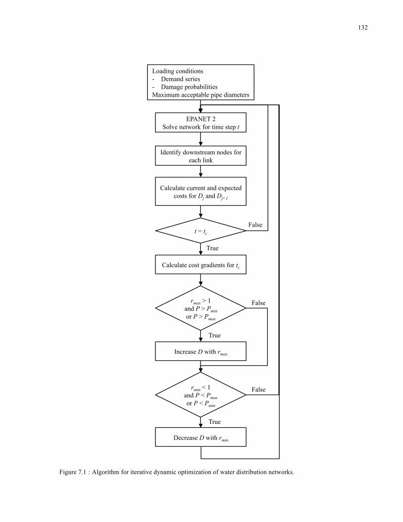
132
Figure 7.1 : Algorithm for iterative dynamic optimization of water distribution networks.
Loading conditions - Demand series - Damage probabilities Maximum acceptable pipe diameters
EPANET 2 Solve network for time step t
Identify downstream nodes for each link
Calculate current and expected costs for Dj and Dj+1
t = tc
Calculate cost gradients for tc
rmax > 1 and P > Pmin or P > Pmax
Increase D with rmax
rmin < 1 and P < Pmax or P < Pmin
Decrease D with rmin
True
False
True
True
False
False

133
Table 7.1: Damage function for Anytown example based on Filion et al. (2007).
Pressure range (m) Conditional probability (per day) Average damages ($M)
P < 14.0 1/3,650 | fire 4.0
14.0 ≤ P < 26.0 1/10 0.02
26.0 ≤ P < 30.0 1/10*(30-P)/4 0.02*(30-P)/4
84.0 ≤ P < 88.0 1/25*(P-84)/4 0.1*(P-84)/4
P ≥ 88.0 1/25 0.1
Damage costs are computed according to the pressures found in the hydraulic simulation. The
costs and probabilities for each pressure range were applied based on the definitions of Filion et
al. (2007). Three types of damages are considered: type-1 damages occurs when the pressure
head falls below 14.0 m at a node and a fire erupts simultaneously; type-2 damages occurs when
the pressure head is between 14.0 and 26.0 m at a node, causing (say) backup pumps on
surrounding industrial properties to fail; type-3 damages occur when pressure head at a node
rises above 88.0 m, potentially leading to a pipe burst. While Filion et al. (2007) applied uniform
damage probabilities for each pressure range, the present study also established adjacent pressure
ranges where probabilities and damage costs decrease linearly (Table 7.1). This more staged
approach not only better resembles real conditions but tend to guide the gradient search.
After defining the demand series and costs, the loads and initial network design are entered into
the EPANET2 network solver (Rossman, 2000). The simulation computes pressures and flows at
nodes and links. The nodes downstream from each link are then successively identified at each
time step, so that the pressure effects of altering pipe diameters can be assessed. At each
iteration, corresponding to one time cycle of the simulation, the ratio between the gradients of
energy dissipation costs, damage costs, and pipe costs is calculated, as indicated in (7.2),
134
ri , j = −EDis i , j − EDis i , j+1( ) ⋅CE ⋅T +CD i , j −CD i , j+1
CP i , j −CP i , j+1 (7.2)
where EDis = energy dissipated (kWh); i = current pipe flows; j = current diameter; j+1 = next
available diameter (larger or smaller); CP = pipe costs.
The ratio is intended to reflect the financial return of investing or disinvesting in pipes. In other
words, the ratio indicates the degree to which other costs, energy and damage, are expected to
increase or decrease given a change in diameter. If pipe diameter is increased, capital costs grow
and this investment would only be worthwhile if other costs, such as energy or damage, are
reduced. Accordingly, the ratio should be greater than 1, in order for a particular increment in
pipe diameter to be beneficial. Conversely,, if pipe diameter is decreased, energy and damage
costs should increase less than the reduction in capital costs, and the ratio should be less than 1.
Accordingly, at each iteration the pipes with the minimum and maximum cost gradient ratios are
identified. The pipe with minimum cost ratio, if below 1, is downsized, whereas the pipe with
maximum cost ratio, if above 1, is upsized. Sizing is altered to the next commercial pipe
diameter. In order to avoid extremely low or high pressures, diameters are also altered if they
surpass constraints even if the cost gradient is unfavorable.
The ratio only considers the primary variables that are expected to change given the adjustment
of pipe diameters. The normally reasonable assumption here is that adjusting one pipe diameter
by one commercial size only marginally affects the flow distribution or the pumping
requirements. Pressures downstream of the altered pipe are recalculated based on this new
demand distribution in order to estimate the revised costs. Nevertheless, after each iteration the
modified network is simulated again and the new distribution is calculated to confirm that the
expected improvement occurs, or to backtrack and undo the modification.
Energy costs are expected to change solely due to modified head losses in the adjusted pipes.
Alternative damage costs are computed with recalculated pressures, assuming that flows are
maintained and only pressures at the nodes downstream of the modified pipe are affected.

135
Furthermore, it is emphasized that for the current exploration the only component of capital costs
that is altered is pipe costs. All costs are extrapolated for the analysis period and discounted to
reflect their present value.
7.4 Anytown Case Study
The proposed method was applied to the Anytown system of Walski et al. (1987). In addition to
being well studied, and having a realistic topological complexity, the Anytown problem accounts
for demand variations (hourly changes and population growth), fire flows, as well as capital and
operational costs. Full details of the system are given in Walski et al. (1987) but are summarized
here for convenience.
The problem consists of proposing new tanks, pumps, as well as pipes that will be laid in a new
area of the city or parallel to existing pipes, in order to meet demands over the next 20 years.
Demands vary throughout the day, yet not seasonally, and grow at different rates, depending on
the location.
In the present study only pipe sizing was optimized, the tank location and sizing recommended
by Gessler (1985) was applied. A schematic representation of the Anytown network is presented
in Figure 7.2. Pipe sizing was optimized given three options, each with different costs, as defined
in the Anytown problem (Walski et al.,1987): installing new pipes (links 54, 68-76); paralleling
old pipes in residential areas (links 36-66); and paralleling old pipes in urban areas (links 2-34,
48). This amounts to 35 pipe diameter variables, each with 10 potential discrete diameters.
Pipe, tank, and pump costs depend on dimensions and location. Following other studies, the cost
of energy is fixed at 0.12 $/kWh, the an annual interest rate at 12%, and the amortization period
at 20 years. While the original Anytown problem does not require the computation of damages, it
sets minimum pressure constraints. Herein, the same interest rate and period were applied to
damage costs.
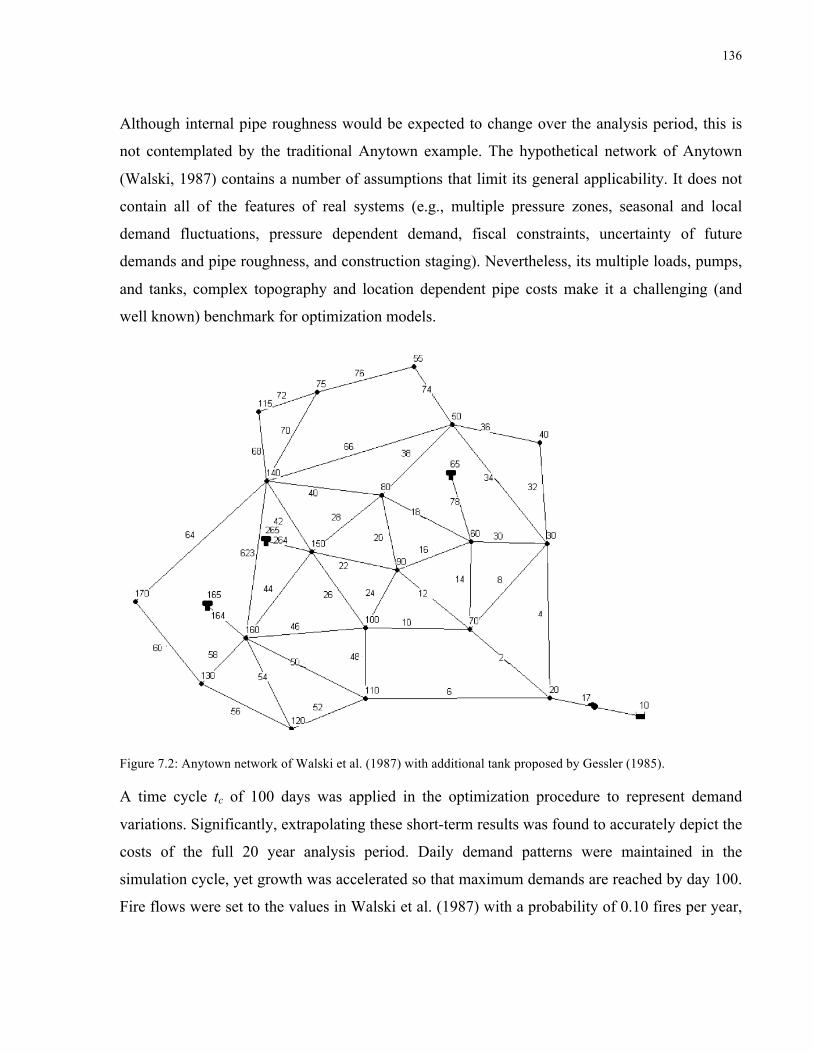
136
Although internal pipe roughness would be expected to change over the analysis period, this is
not contemplated by the traditional Anytown example. The hypothetical network of Anytown
(Walski, 1987) contains a number of assumptions that limit its general applicability. It does not
contain all of the features of real systems (e.g., multiple pressure zones, seasonal and local
demand fluctuations, pressure dependent demand, fiscal constraints, uncertainty of future
demands and pipe roughness, and construction staging). Nevertheless, its multiple loads, pumps,
and tanks, complex topography and location dependent pipe costs make it a challenging (and
well known) benchmark for optimization models.
Figure 7.2: Anytown network of Walski et al. (1987) with additional tank proposed by Gessler (1985).
A time cycle tc of 100 days was applied in the optimization procedure to represent demand
variations. Significantly, extrapolating these short-term results was found to accurately depict the
costs of the full 20 year analysis period. Daily demand patterns were maintained in the
simulation cycle, yet growth was accelerated so that maximum demands are reached by day 100.
Fire flows were set to the values in Walski et al. (1987) with a probability of 0.10 fires per year,

137
as suggested by Filion et al. (2007). The occurrence of fires during the simulation time cycle tc is
stochastically established with a random number generator.
Although hourly time cycles clearly do not fully represent the variation of flows during the
analysis period and may not produce uniformly accurate good results, the assertion here is their
advantages outweigh their faults. That is, that a “compressed” approach to time variations can
be used to generate useful approximations to a more generally valid solution, thus creating a
provisional solution that can significantly speed the overall optimization process. Accordingly,
hourly iterations were initially used to generate a rough solution which was then optimized with
the 100 day time cycle tc.
In order to assess the effect of different conditions on the solution, variations of the problem
were also optimized. For instance, reduced population growth, consumer water saving, or utility
led conservation initiatives could lower water consumption. Damage costs are also inevitable
uncertain and depend on the utility’s valuation of damages, its aversion to risk and many other
factors include the timing of damage and the ever-changing vulnerability of users. Accordingly,
two additional scenarios were optimized, with final demand reduced by 10%, and with doubled
damage costs.
7.5 Results and Discussion
Results of the optimization process are compared to those of Gessler (1985) in Table 7.2, which
assumed the same tank and pump sizing and location. The proposed solution has a total cost of
$M 16.5, which only 2% higher than the $M 16.3 cost of Gessler’s (1985) solution. This is due
to higher capital costs, which in turn reduce damage costs. Despite this investment in larger
pipes, however, energy costs remain virtually unchanged. Walski et al. (1987) also noted the low
sensitivity of Anytown energy costs to pipe sizing, except when it affects pump efficiency.
Therefore, network optimization, in this case, is largely concerned with selecting the smallest
pipe diameters that avoid exceptionally high costs or exceed pressure constraints.

138
Although the proposed solution does not quite achieve Gessler’s (1985) low cost, it comes quite
close using a less computationally intensive process. The reported solution to the original
Anytown problem was reached after 24,000 hourly iterations of the gradient technique, that
converged to an approximate solution, and subsequent 33 100-day iterations, totaling almost 12
years of hydraulic simulations. Therefore, in order to reach its solution the network was modeled
for fewer years than its total analysis period, 20 years. This took about 1.2 h on a notebook with
a 1.9 GHz processor in Windows Vista. Compared to previous optimization studies of the
Anytown network described in the literature review, even single trials for optimizing pipe sizing,
this represents a notable reduction in computational costs. Approximating the objective function
through shorter period analyses is a real simplification. This acceleration technique can
obviously be applied to other optimization methods too. The decision to apply the proposed
gradient optimization method will depend on the complexity of the problem and, thus, the trade-
off between computational costs and potential savings.
Table 7.2: Pipe sizes and expected costs for Anytown design solutions: (I) original problem, (II) 10% decreased demand growth, and (III) doubled damage costs.
Pipe Diameters (mm) Solutions 2 4 6 12 18 30 32 34 42 44 48 50 Gessler (I) 1 356 610 1 1 254 1 1 356 457 1 610 Gradient (I) 356 305 457 305 203 203 203 203 1 1 254 305 Gradient (II) 305 305 406 305 203 203 203 203 1 1 254 254 Gradient (III) 356 305 457 305 203 203 203 203 1 1 254 305
Table 7.2 cont.: Pipe sizes and expected costs for Anytown design solutions: (I) original problem, (II) 10% decreased demand growth, and (III) doubled damage costs.
Costs ($M) 52 54 58 60 68 70 72 74 76 Capital Energy Damage Total 1 203 406 356 305 305 152 356 152 5.8 6.8 3.6 16.3
254 305 1 152 356 152 305 610 457 6.2 6.8 3.5 16.5 254 356 203 152 356 152 254 508 406 6.0 6.7 3.8 16.5 254 356 254 254 356 152 203 610 406 6.4 6.8 6.8 20.0
The various uncertainties regarding the future of water distribution systems also make it more
difficult to compare network solutions. Predicted costs are attached to a probability and margin
of error, which mean they in fact promise a range of potential future costs. Furthermore, other
139
decisions taken as immutable in many optimization methods can generate more savings. This
undermines the high computational efforts of optimization methods, which might be selecting
pipe sizes for systems with sub-par pump and storage design. For instance, the original solutions
to the Anytown problem (Gessler, 1985; Brill et al., 1985; Morgan and Goulter, 1985; Ormsbee,
1985) compared by Walski et al. (1987) consist of distinct tank locations and sizes, and incur
costs that differ by up to 12%. A non-computationally intensive optimization process, such as the
one proposed, could facilitate greater analysis of more design, operation, and management
scenarios. If applied as part of a broader optimization process that compares multiple scenarios,
it could helpfully supplement engineering judgement and experience.
In order to test the proposed gradient method and evaluate the costs of potential uncertainties,
two additional scenarios were optimized: a 10% decreased demand growth (II), and a run with
doubled damage costs (III), shown in Table 7.2. Although many other uncertainties exist, these
are variables that greatly depend on future infrastructure conditions, user behavior, and utility
operations. The increasing focus on water conservation, as an environmental, as well as a cost
reducing measure focus on water conservation, as an environmental, as well as a cost reducing
measure, has led to lower demands, sometimes unexpectedly, rendering networks overdesigned.
Accordingly, if this demand management is planned, the optimal design should differ. As
expected, the reduced demand scenario resulted in a network with smaller pipes, but increased
damages. Yet, total costs did not differ greatly. Nevertheless, if the network optimized for the
original scenario were to experience reduced demands, total costs would be expected to me
marginally (2%) higher. With doubled damage costs, the proposed gradient method generated a
network with larger diameters and reduced damages. Therefore, the optimization technique
responded to the system modifications and generated expected adjustments in network designs.
Although designs are similar, pipe diameters only differ by one or two sizes, they reflect a
different balance between capital costs and damages.
Because fires are stochastically generated in the model, a different random seed can also affect
costs, and thus the solution. Altering the set of stochastically generated fires was found to
potentially change solution costs by around 2%. The network was also optimized for one set of
140
fires and checked for another. Similarly, this was found to change costs by approximately 2%.
Therefore, the uncertainty in future damages affects the solution and should be investigated in
future studies. Nevertheless, the solution performance was shown to be stable with a new set of
fires.
7.6 Initial Assessment of the Proposed Methodology
As other heuristic methods, the proposed gradient search technique does not guarantee an
optimal solution and is sensitive to the parameters chosen. In the present case, total costs are a
function of user demands, fire flows, pipe costs, energy rates, damage costs, and pressure limits.
Future energy rates are uncertain and depend on a number of factors, such as available fuels,
power generation, weather conditions, regulations. and the global economy. Pressure limits are
based on safety standards that vary by system, and transgressing them does not necessarily
translate into real damages. Damage costs, applied less in other optimization methods, depend
not only on the network and its operations, which affect the probability of damages, but also on
stakeholder valuation of damages, particularly for those sustained by humans.
The damage costs suggested by Filion et al. (2007) and applied herein comprise three types of
damages: loss of life and property, interruption of industrial production, and damage to system
pipes. The problem, as currently formulated, thus balances potential costs of loss of life with
system costs, which is controversial. Nevertheless, other methods do this, yet implicitly by
balancing costs with pressures, resilience, or reliability. Decision makers should, thus,
understand and make explicit the assumptions attached to pressure limits and costs. These should
be established according to system properties and stakeholder risk aversion.
If applied to a real network, the proposed method would require the assessment of the damage
probability density functions, and an evaluation of damage costs. Future studies can analyze
these system properties and perhaps identify commonalities that can facilitate approximations.
This information would not only be useful in the design phase, as applied here, but also during

141
operations and planning. Other costs would need to be included in real system decision making
as well, such as water treatment, maintenance, and environmental damages.
The proposed optimization technique has a positional bias, which means the final solution is
influenced by the initial design. Because pipe sizes are set to their maximum value in the initial
iteration, solutions tend towards larger pipe diameters. This, nevertheless, generates more robust
networks. Furthermore, the short time cycles used to represent the full analysis period, slightly
overestimate damages since demands vary more often, which also leads to larger diameters. In
order to reduce these discrepancies, more initial designs could be used as well as longer time
cycles. However, the parameters applied herein generated near optimal solutions with lower
damage costs than Gessler (1985). In other applications, these will need to be chosen according
to the complexity and demand variation of the system.
The cost gradient technique seems more intuitive than many optimization methods, facilitating
its application and adaptation by water utilities. Because it is also less computationally intensive
than most other methods, more scenarios and alternatives can be assessed, enabling utility
decision-making, which is obviously concerned with more than pipe sizing, infrastructure costs,
and energy costs. Different from other gradient techniques, the present method accepts varying
loads. Furthermore, its inclusion of damage costs helps balance system costs and resilience.
The proposed method extends previous optimizations processes. Nevertheless, the optimization
of water distribution systems, due to their complexity, is inherently challenging. The core
concept of optimization, that of achieving the “best” solution, is clearly disputable. The long life
cycle of the infrastructure and its interaction with an evolving and highly human context produce
multiple uncertainties. The models that represent this reality must balance tensions between
simplicity and accuracy, generality and specificity, internal and external parameters (i.e., what is
included in the model and what is asked of it), as well as accepted and rejected conditions (i.e.,
what of the system is accepted and modified by applying the model).
142
7.7 Conclusions
A cost gradient search technique is used to iteratively model long-term network hydraulics with
varying loads using shorter time cycles and to adjust pipe diameters in order to minimize system
costs (capital, operational, and damage). The research extends previous studies of capital-cost
single-load gradient techniques and those with expected annual damages, in order to develop a
less computationally intensive optimization method. When applied to the well-known network of
Anytown, results indicated that shorter time cycles can be used to approximate full period costs.
Additionally, the technique can be applied to different scenarios and can generate near optimal
solutions. It is, thus, useful in cases where more computationally intensive methods are infeasible
or cannot generate much greater savings, such as optimizing pipe diameters of complex systems
with varying loads, and comparing multiple strategies (infrastructure, operational, and
management). Future studies are required to apply the proposed technique to real systems in
order to further verify its usefulness and applicability. Furthermore, a detailed study of system
uncertainties and their effect on system costs must eventually be performed in order to better
prioritize computational efforts.
143
8 Conclusions and Future Steps This thesis seeks to take a metaphorical step back in order to gain a panoramic view of the water
supply system and better align the research with utility needs. The need for a better
understanding of not only the infrastructure, but also of system requirements, risks, costs and
stakeholders becomes clear from this view. Previous chapters have studied different components
of water distribution systems, and their connections. They only begin to explore the complexities
that abound within these systems, but they address the main current issues from a systems
perspective by analysing system interconnections and applying readily available resources.
The proposed tools were envisioned to address current issues of North American water
distribution systems, particularly those in Ontario, Canada, and to lessen the gap between
research and application. Accordingly, they were developed to be applied by engineers, planners,
and managers with current modeling and data collection practices. The issues addressed by them
include water scarcity, disconnection between utilities and stakeholders, inefficient energy use,
failure to comprehensively assess infrastructure performance of complex systems, and high
computational expenses of optimizing water network design. These are each related to a gamut
of other issues, such as leakage, aging infrastructure, high expansion costs, and short-termism.
Nevertheless, the tools are not meant to solve all problems faced by water distribution systems,
but to begin to shift perspectives, address important issues systemically, and motivate the quest
for sustainability. Accordingly, the key message of this study is the benefit of applying systems
thinking to the development of new solutions for sustainable water distribution systems.
8.1 Summary of Contributions and Conclusions
The major contribution of the thesis to the field of water distribution system analysis has been
the development of tools that take into account the complex interconnections of these systems
and facilitate decision-making by collecting, integrating, analysing, and re-interpreting readily
available data and models.
144
Each chapter or tool has led to specific contributions, described below.
1. Chapter 2 compares different definitions of sustainability and argues that the various
connections between objectives of sustainable systems call for integrated approaches. In
order to facilitate a systemic analysis, the connections between components of water
distribution systems are mapped. This facilitates the visualization of feedback loops,
hubs, and potential cascade effects. Subsequent chapters explore how these connections
can inform decisions, and how the decisions affect the connected components.
2. Chapter 3 proposes an approach for water demand management. The chapter is based on
the manuscript entitled “Building an Integrated Water-Land Use Database for Defining
Benchmarks, Conservation Targets, and User Clusters”, published in the Journal of
Water Resources Planning and Management, and reproduced with permission from
ASCE. The issue of limited water resources is addressed by identifying factors that
motivate water consumption and users that consume more water than expected, given
their characteristics. Demographic, land use, and water consumption data are linked in an
integrated database, which is used to define water use metrics, benchmarks, conservation
targets, and customer segments. The approach was applied to the cities of Barrie, Guelph,
and London, ON. The metrics are shown to normalize water consumption and facilitate
the comparison of water use between sectors or even utilities. The benchmarks and
conservation targets further facilitate demand planning and communication regarding
conservation. Furthermore, customer segments are defined through a clustering analysis
which indicates that users within the same or similar property code tend to cluster
together. Therefore, property codes can be used to classify customers if more detailed
data is not available.
3. Chapter 4 develops a survey for collecting user feedback on expectations of service in
order to gauge the correlation between user and utility concerns, and support the
improvement of the water utility’s business model. The chapter is based on the
manuscript entitled “Collectively Re-envisioning the Water Utility Business Model”,
submitted to Water Resources Management. It furthers the analysis of the demand side

145
through qualitative research. Questions relate to user demographics, characteristics,
awareness, concerns, motivations, priorities, communication, and water system related
preferences. The survey was conducted with residential water users in the City of Guelph,
ON. As expected, results highlight user concern with water scarcity, an issue that has
been regularly addressed by the local utility and is the focus of the City’s latest Water
Supply Master Plan Update. Nevertheless, other issues were also identified, such as
concerns with water quality, aging infrastructure, and costs, as well as low awareness of
many system components, calling for further attention by the utility. Furthermore,
different user types were found to prefer distinct communication channels, confirming the
need for alternative channels in order to reach and receive feedback from users. The
business model perspective, applied in discussing results and potential improvements to
the utility, was found to motivate a systems approach and warrant a deeper understanding
of the users and the service they require.
4. Chapter 5 proposes energy metrics in order to assess the energy efficiency of water
networks and their components. The chapter is based on the manuscript entitled “Energy
Metrics for Water Distribution System Assessment: A Case Study of the Toronto
Network”, submitted to the Journal of Water Resources Planning and Management. The
metrics describe how energy is supplied, dissipated, lost, and delivered, throughout the
system, on both a local and global (system-wide) scale in different operational scenarios.
These are not only indicators of electricity use, but also of system capacity, efficiency,
burst potential, and greenhouse gas emissions. Furthermore, the comparison of
component metrics allows for the identification of specific pipes, tanks, or pumps where
changes would be most beneficial. The proposed energy metrics were applied to a case
study of the Toronto water distribution system. Significantly, results indicate that, on
average, less than 27% of energy supplied to the system is delivered to the users in the
form of pressure and flow. This inefficiency has important economic and environmental
repercussions. Nevertheless, it was found that changes to operations, such as pump
scheduling, could increase efficiency without considerably affecting system pressures.

146
5. Chapter 6 proposed performance metrics for assessing the performance of networks with
multiple loading conditions. The chapter is based on the manuscript entitled
“Performance Index for Water Distribution Networks Under Multiple Loading
Conditions”, submitted to the Journal of Water Resources Planning and Management.
The metrics represent system reliability, vulnerability, resilience, and connectivity. .
These are themselves based on the energy efficiency, hydraulic capacity and structural
ability of the system to deliver water under a range of conditions. The metrics were
applied to two example networks and variations of these, enabling the assessment of their
relevance, their sensitivity to system changes, and permitting a comparison to existing
metrics. The proposed performance index generally follows a similar trend as the existing
indices, increasing with network pressure. Nevertheless, it varies differently and
penalizes networks with unnecessarily high pressures. Because the index is based on
energy and demand efficiency metrics, it automatically complies with the energy and
mass balances of the network. Moreover, the new metric is easily interpreted and can be
applied to various systems, whether complex or involving multiple scenarios.
6. Chapter 7 presents a cost gradient search technique that optimizes pipe sizing of networks
with varying loads. The chapter is based on the manuscript entitled “Cost Gradient
Search Optimization Technique for Water Distribution Networks with Varying Loads”,
submitted to the Journal of Water Resources Planning and Management. It seeks to
reduce the computation time of optimizing water distribution networks with varying
demands by using a sequence of shorter time cycles to approximate a fuller range of
costs. This should facilitate the application of the method to a broader optimization
process through which multiple strategies (infrastructure, operational, and management)
are compared. The technique was applied to the well-known network of Anytown.
Results indicate that the technique can effectively be applied to different scenarios and
can generate robust solutions. Furthermore, its lower computational intensity should
facilitate its application as part of a broader optimization process and thus better enable
the assessment of more storage, pumping, and control alternatives.

147
8.2 Future Research
Previous chapters have proposed decision support tools and applied them to real or example
systems. In order to further validate their applicability and begin to benchmark water use,
energy, and performance metrics, future research should apply the tools to other examples and
case studies. The challenges encountered in applying the tools, limitations of these approaches,
and persisting questions within each chapter have also inspired potential extensions to the
present research.
1. The conceptual map of water system components and their connections, presented in
Chapter 2, although useful in guiding decisions does not describe the degree to which
components influence each other. Future research should better characterize these
connections, qualitatively and quantitatively.
2. The preparation of the data in Chapter 3, was found to be the most time consuming phase
of the process, particularly because information was integrated from different sources.
Future work can seek to standardize inputs and facilitate the integration of public data, in
order to build ever more interoperable databases.
3. The proposed database integrated water billing, land use, and demographic information,
Nevertheless, other factors can influence water consumption and inform conservation
strategies. Future studies can integrate additional data (e.g., unit counts, industrial
classification, participation in programs, income) in order to better understand water user
segments.
4. The survey in Chapter 4 was conducted with residential water users only. Nevertheless,
the characteristics and opinions of industrial, commercial, and institutional water users
would likely differ and should be surveyed and compared in future research.
Furthermore, results indicated that the older population was more likely to participate in

148
the telephone survey. Therefore, different feedback channels should also be used in the
future to gain input from the different customer segments.
5. The proposed energy and performance metrics were shown to be useful indicators of
energy efficiency, infrastructure performance, and costs. If applied in the future to
support decision-making, they should be balanced with other considerations including
costs, pressure constraints, and other social and environmental criteria.
6. Even though the performance metrics described in Chapter 6 are computed with two
failure scenarios: fire flow during maximum demand, and pipe break during peak
demand, for the initial assessment of the metrics, they can be applied to multiple
scenarios, including simultaneous failures. Therefore future studies can analyse real
networks with multiple scenarios.
7. Future research can also apply the proposed metrics and indicators, chapters 3 to 6, in
designing a rating scheme for water distribution systems.
8. Chapter 7 argues that the high computational intensity of previous complex pipe sizing
optimization techniques might not translate into significant savings, given the importance
of other design components, such as pump and tank sizing, as well as the various
uncertainties of the system. Future research should study the effects of design decisions
and uncertainties on total costs, in order to better prioritize computational efforts.
9. The proposed optimization technique minimized capital, energy, and damage costs. If
applied in the future to real systems, other costs would need to be included as well, such
as water treatment, maintenance, and environmental damages. Furthermore, certain utility
and stakeholder objectives might be difficult to valuate, but a qualitative comparison of
alternatives could facilitate decision-making.
In addition to further applying the proposed tools and extending upon the present research, future
research should review water distribution assumptions and rethink design objectives. The

149
constraints imposed by design standards and utility norms are pivotal to decision making, yet are
generalized and many times based on older paradigms.

150
References
Aini, M.S., Fakhru’L-Razi A., Suan, K. S. (2001). Water Crisis Management: Satisfaction Level,
Effect and Coping of the Consumers. Water Resources Management 15: 31-39. Alegre H., Hirner W., Baptista J.M. Parena R. (2000) Performance Indicators for Water Supply
Services. IWA Manual of Best Practice, London, UK. Alegre H., Baptista J.M., Cabrera Jr., E., Cbullo, F., Duarte, P., Hirner W., Parena R. (2006)
Performance Indicators for Water Supply Services. IWA Manual of Best Practice, 2 ed., London, UK.
Alperovits, E., Shamir, U. (1977). Design of Optimal Water Distribution Systems. Water Resources Research. 13(60): 885-900.
Aly, A. H., Wanakule, N. (2004). Short-Term Forecasting for Urban Water Consumption. Journal of Water Resources Planning and Management 130: 405-410.
American Water Works Association. (1995). Distribution System Performance Evaluation. AWWA.
American Water Works Association. (2012). Burried no Longer: Confronting America’s Water Infrastructure Challenge. AWWA.
Amit, R. K. and Ramachandran, P. (2010). A Fair Contract for Managing Water Scarcity. Water Resources Management. 24: 1195-1209.
Atkinson, S., Farmani, R., Memon, F. A., Butler, D. (2014) Reliability Indicators for Water Distribution System Design: Comparison. Journal of Water Resources Planning and Management, 140 (2), 160-168.
Awumah, K., Goulter, I., Bhatt, and S. K. (1990). Assessment of reliability in water distribution networks using entropy based measures. Stochastic Hydrology and Hydraulics, 4, 309-320.
Babayan, A., Kapelan, Z., Savic, D., Walters, G. (2005). Least-Cost Design of Water Distribution Networks under Demand Uncertainty. Journal of Water Resources Planning and Management. 131 (5): 375-382.
Bakker, K., Cameron, D. (2005). Governance, business models and restructuring water supply utilities: recent developments in Ontario, Canada. Water Policy. 7 (5): 485-508.
Baños, R., Reca, J., Martínez, J., Gil, C., and Márquez, A. (2011). Resilience indexes for water distribution network design: A performance analysis under demand uncertainty. Water Resources Management, 25(10), 2351–2366.
Biomimicry 3.8 Institute. (2011). Life’s Principles: Design Lessons from Nature. Biomimicry 3.8 Institute.

151
Blokker, E. J. M., Vreeburg, H. G., van Dijk, J. C. (2010). Simulating Residential Water Demand with a Stochastic End-Use Model. Journal of Water Resources Planning and Management, 136 (1), 19-26.
Boulos, P. F., Bros, C. M. (2010). Assessing the carbon footprint of water supply and distribution systems. American Water Works Association Journal, 102 (11): 47-54.
Boyle, C. E., Eskaf, S., Tiger, M. W., Hughes, J. A. (2011). Mining water billing data to inform policy and communication strategies. American Water Works Association Journal. 103 (11): 45-58.
Brill, E. D., Liebman, J. C, and Lee, H. L. (1985). Optimization of looped water distribution networks, Computer applications in water resources, H. C. Torno, Ed., ASCE, New York, N.Y., 569-571.
Bristow D., Richman W., Kirsh .A, Kennedy C. A., Pressnail, K. D. (2011). Hour-by-Hour Analysis for Increased Accuracy of Greenhouse Gas Emissions for a Low-Energy Condominium Design. Journal of Industrial Ecology, 15: 381-393
Brooks, D. B. (2006). An Operational Definition of Water Demand Management. Water Resources Development, 22 (4), 521-528.
Brun, M., Sima, C., Hua, J., Lowey, J., Carroll, Suh, E., and Dougherty, E. R. (2007). Model-based evaluation of clustering validation measures. Pattern Recognition, 40 (3): 807-824.
Cabrera, E., Pardo, M. E., Cobacho, R., Cabrera Jr., Enrique. (2010). Energy Audit of Water Networks. Journal of Water Resources Planning and Management, 136 (6): 669-677.
Cahill, R., and Lund, J. (2013). Residential Water Conservation in Australia and California. Journal of Water Resources Planning and Management 139 (1), 117-121.
City of Toronto, Manager’s Office. (2012). 2010 Performance Measurement and Benchmarking report. Toronto.
City of Toronto, Energy and Waste Management Office, Environment and Energy Division. (2014). Annual Energy Consumption and Greenhouse Gas Emissions. City of Toronto, Toronto.
Colombo, A. F., Karney, B. W. (2002). “Energy and costs of leaky pipes: Toward a comprehensive picture.” Journal of Water Resources Planning and Management, 128 (6): 441-450.
Colombo, A. F., Karney, B. W. (2003). The labyrinth of water distribution systems: Demand, energy, and climate change. First International Conference on Pumps, Electromechanical Devices and Systems (PEDS), April 22-25, 2003, Valencia, Spain.
Conrad, S., Pipher, J., Haider, W., Rutherford, M., Yates, D. (2013). Okanagan Water Study: Resident Descriptive Statistics. Simon Fraser University.
Corne, D.W., Jerram, N., Knowles, J.D., Oates, M.J., 2001. PESA-II: region-based selection in multiobjective optimization. In: GECCO, vol. 1, pp. 283–290.

152
Creaco, E., Fortunato, A., Franchini, M., Mazzola. M. R. (2014). Comparison between entropy and resilience as indirect measures of reliability in the framework of water distribution network design. 12th International Conference on Computing and Control for the Water Industry, Perugia, Italy. Procedia Engineering 70: 379-388.
Creaco, E., Franchini, M., Walski, T. (2014a). Accounting for Phasing of Construction within the Design of Water Distribution Networks. Journal of Water Resources Planning and Management, 140 (5): 598-606.
Creaco, E., Franchini, M., Walski, T. (2014b). Taking Account of Uncertainty in Demand Growth When Phasing the Construction of a Water Distribution Network. Journal of Water Resources Planning and Management, 10.1061/(ASCE)WR.1943-5452.0000441, 04014049-1.
Creaco, E., Franchini, M., Todini, E. (2014c). The combined use of resilience and loop diameter uniformity as a good indirect measure of network reliability. Urban Water Journal. 10.1080/1573062X.2014.949799, 10-15.
Cutore, P., Campisano, A., Kapelan, Z., Modica, C., Savic, D. (2008). Probabilistic Prediction of Urban Water Consumption Using the SCEM-UA algorithm. Urban Water Journal 5: 125-132.
Di Nardo, A., Di Natale, M., Santonastaso, G. F., Tzatchkov, V. G., and Alcocer-Yamanaka, V. H. (2014). Water Network Sectorization Based on Graph Theory and Energy Performance Indices. Journal of Water Resources Planning and Management, 140(5), 620–629.
di Pierro, F., Khu, S. T., Savic, D., Berardi, L. (2009). Efficient multi-objective optimal design of water distribution networks on a budget of simulations using hybrid algorithms. Environmental Modelling &Software, 24 (2): 202-213.
Donkor, E. A., Mazzuchi, T. A., Soyer, R., Roberson J. A. (2014). Urban Water Demand and Forecasting: Review of Methods and Models. Journal of Water Resources Planning and Management, 140 (2), 146-159.
Dziegielewski, B., and Kiefer, J.C. (2010). Water Conservation Measurement Metrics: Guidance Report. AWWA, Denver, CO.
Electric Power Research Institute. (2002). Water & Sustainability (Volume 4): U.S. Electricity Consumption for Water Supply & Treatment - The Next Half Century. Palo Alto, California.
Environment Canada. (2010). Municipal water use report: Municipal water use, 2006 statistics. Environment Canada, Gatineau, QC, Canada.
Eusuff, M. M., Lansey, K. E. (2010). Optimization of Water Distribution Network Design Using the Shuffled Frog Leaping Algorithm. Journal of Water Resources Planning and Management. 129 (3): 210-225.

153
Farmani, R., Walters, G. A., Savic, D. A. (2005). Trade-off between Total Cost and Reliability for Anytown Water Distribution Network . Journal of Water Resources Planning and Management, 131 (3): 161-171.
Fiering, M. B. (1982a). Alternative indices of resilience. Water Resources Research, 18(1), 33. Fiering, M. B. (1982b). Estimating resilience by canonical analysis. Water Resources Research,
18(1), 51. Filion, Y. R., Adams, B. J., Karney, B. W. (2007). Stochastic Design of Water Distribution
Systems with Expected Annual Damages. Journal of Water Resources Planning and Management. 133 (3): 244-252.
Filion, Y. R. (2008). Impact of Urban Form on Energy Use in Water Distribution Systems. Journal of Infrastructure Systems, 14 (4), 337-346.
Fischer, J. M., Amekudzi, A. (2011). Quality of Life, Sustainable Civil Infrastructure, and Sustainable Development: Strategically Expanding Choice. Journal of Urban Planning and Development. 137 : 39-48.
Foellmi, R., Meister, U. (2012). Enhancing the Efficiency of Water Supply – Product Market Competition Versus Trade. Journal of Industry, Competition, and Trade, 12: 299-324.
Franceschini, F., Galetto, M., Turina, E. (2010). Water and Sewage Service Quality: A Proposal of a New Multi-Questionnaire Monitoring Tool. Water Resources Management, 24 : 3033-3050.
Fu, G., Kapelan, Z., Reed, P. (2012). Reducing the Complexity of Multiobjective Water Distribution System Optimization through Global Sensitivity Analysis. Journal of Water Resources Planning and Management, 138 (3): 196-207.
Fu, G., Kapelan, Z., Kasprzyk, J., and Reed, P. (2013). Optimal Design of Water Distribution Systems Using Many-Objective Visual Analytics.” Journal of Water Resources Planning and Management, 139(6), 624–633.
Fujiwara, O., Khang D. B. (1990). A two-phase decomposition method for optimal design of looped water distribution networks. Water Resources Research. 26 (4) 539-549.
Gay, L. F., Sinha, S. K. (2012). “Measuring Energy Efficiency in Urban Water Systems Using a Mechanistic Approach.” Journal of Infrastructure Systems, 18 (2): 139-145.
Gessler, J. (1985). Pipe network optimization by enumeration. Computer applications in water resources, H. C. Torno, Ed., ASCE, New York, N.Y., 572-581.
Ghimire, S. R., and Barkdoll, B D. (2010). Sensitivity analysis of municipal drinking water distribution system energy use to system properties. Urban Water Journal, 7 (4), 217-232.
Giacomini, M. H., Kanta, L., Zechman, E. M. (2013). Complex Adaptive Systems Approach to Simulate the Sustainability of Water Resources and Urbanization. Journal of Water Resources Planning and Management 139 (5): 554-564.

154
Gleick, P. H., Haasz, D., Henges-Jeck, C., and Srinivasan, V., Wolff, G., Cushing, K. K., Mann, A. (2003). Waste Not, Want Not: The Potential for Urban Water Conservation in California. Pacific Institute, Oakland, CA.
Gomes, H. P., Bezerra, S. T. M., Carvalho, P. S. O., Salvino, M. M. (2009). Optimal dimensioning model of water distribution systems. Water SA 35(4): 421-431.
Goulter, I., Walski, T. M., Mays, L. W., Sakarya, A. B. A., Bouchart, F., and Rung, Y.K. (2004). Hydraulic Design of Water Distribution Storage Tanks. Chap. 18 Mays, L. W. Water Distribution Systems Handbook. McGraw Hill, New York, NY.
Haghighi, A., Samani, H. M. V., Samani, Z. M. V. (2011). GA-ILP Method for Optimization of Water Distribution Networks. Water Resources Management 25 (7) :1791-1808.
Hashimoto, T., Stedinger, J. R., and Loucks, D. P. (1982). Reliability, resiliency and vulnerability criteria for water resource system performance evaluation. Water Resources Research, 18(1), 14–20.
Heller, M., Von Sacken, E. W., Gerstberger. (1999). Water utilities as integrated businesses. Journal American Water Works Association. 91 (11): 72-83.
Hillenmeyer, M. (2005) Machine Learning. Stanford University, Stanford, CA. Ho, M. W., and Ulanowicz, R. (2005). Sustainable systems as organisms? BioSystems 82, 39-51.
Holling, C. S. (1973). Resilience and Stability of Ecological Systems. Annual Review of Ecology and Systematics, 4, 1–23.
Holling, C. S. (1996). Engineering resilience versus ecological resilience. Engineering within ecological constraints, P. C. Schulze, ed., National Academy Press, Washington, D.C., 31–44.
Hussey, K., and J. Pittock. (2012). The Energy–Water Nexus: Managing the Links between Energy and Water for a Sustainable Future. Ecology and Society, 17 (1), 31.
HydraTek. (2013). Toward Municipal Sector Conservation: A Pump Efficiency Assessment and Awareness Pilot Study. Hydratek, Toronto, Canada.
Institute for Sustainable Infrastructure, Zofnass Program for Sustainable Infrastructure. (2012) ENVISION Version 2.0: A Rating System for Sustainable Infrastructure. ISI, Washingtion,.
International Standards Organization - ISO. (2008). Guide for Determination of Needed Fire Flow. ISO Properties Inc., Jersey City, New Jersey.
Jayaram, N., and Srinivasan, K. (2008). Performance-based optimal design and rehabilitation of water distribution networks using life cycle costing. Water Resources Research, 44(1), W01417.
Jorgensen, B., Graymore, M., O’Toole, K. (2009). “Household water use behavior: An integrated model.” Journal of Environmental Management, 91 (1), 227-236.

155
Katifori, E., Szöllosi, G. J., Magnasco, M. O. (2010). Damage and Fluctuations Induce Loops in Optimal Transport Networks. The American Physical Society 104 (4): 1-4.
Kettler, A. J., Goulter, I. C. (1985). An analysis of pipe breakage in urban water distribution networks. Canadian Journal of Civil Engineering, 12: 286-293.
Klein, R. J. T., Nicholls, R. J., and Thomalla, F. (2003). Resilience to natural hazards: How useful is this concept? Environmental Hazards, 5(1), 35–45.
Kleine, A., von Hauff, M. (2009). Sustainability-Driven Implementation of Corporate Social Responsibility: Application of the Integrative Sustainability Triangle. Journal of Business Ethics, 85: 517-533.
Klemes, V., Srikanthan, R., and McMahon, T. A. (1981). Long-memory flow models in reservoir analysis: What is their practical value? Water Resources Research, 17(3), 737–751.
Knowles, J., 2006. ParEGO: a hybrid algorithm with on-line landscape approximation for expensive multiobjective optimization problems. IEEE Transactions on Evolutionary Computation, 10 (1): 50–66.
Kollat, J. B., and Reed, P. M. (2006). “Comparing state-of-the-art evolutionary multi-objective algorithms for long-term groundwater monitoring design.” Advances in Water Resources, 29(6), 792–807.
Kumar G., Karney B. W. (2012). Natural Cities, Unnatural Energy? In: Stefanovic I L, Scharper S B, The Natural City: Re-envisioning the Built Environment, University of Toronto Press, Toronto
Lambert, A. O, (2000). What do we know about pressure: leakage relationships in distribution system? Proceedings of the IWA conference on System Approach to Leakage Control and Water Distribution Systems Management. Brno, Czech Republic
Lambert A, Huntington D and Brown T.G. (2000): Water Loss Management in North America – Just How Good is it? Proceedings of the American Water Works Association Distribution Systems Symposium, New Orleans,
Lambert A. O., McKenzie R. D. (2002). Practical Experience in using the Infrastructure Leakage Index. International Water Association Conference. ‘Leakage Management: A Practical Approach’, Cyprus.
Lee, J. A., and Verleysen, M. (2002). Self-organizing maps with recursive neighborhood adaptation. Neural Networks, 15 (8-9), 993-1003.
Liner, B., deMonsabert, S. (2011). Balancing the Triple Bottom Line in Water Supply Planning for Utilities. Journal of Water Resources Planning and Management, 137: 335- 342.
Loucks, D. P., and van Beek, E. (2005). Water resources systems planning and management, United Nations Educational, Scientific and Cultural Organization (UNESCO), Paris.
Maas, C. (2009). H2Ontario: A Blueprint for a Comprehensive Water Conservation Strategy. Water Sustainability Project, POLIS Project on Ecological Governance. Victoria, BC, Canada.
156
Maidment, D. R. (2008). Bringing Water Data Together. Journal of Water Resources Planning and Management, 134 (2), 95-96.
Marques, J., Cunha, M., Savic, D. (2014). Using Real Options in the Optimal Design of Water Distribution Networks. Journal of Water Resources Planning and Management. 10.1061/(ASCE)WR.1943-5452.0000448, 04014052-1.
McMahon, T. A., Adeloye, A. J., and Sen-Lin, Z. (2006). Understanding performance measures of reservoirs. Journal of Hydrology (Amsterdam), 324 (2006), 359–382.
McMichael, A. J., Butler, C. D., Folke, C. (2003). New Visions for Addressing Sustainability. Science 302 : 1919- 1920.
Michalski, R., 2000. Learnable evolution model: evolutionary processes guided by machine learning. Machine Learning 38 (1–2), 9–40.
Ministry of Municipal Affairs and Housing Ontario – MAH (2012). List of Measures for 2011 Reporting. Ontario.
Monbaliu, J., Jo, J. H., Fraisse, C. W., Vadas, R. G. (1990). Computer aided design of pipe networks. Water resource systems application, S. P. Simonovic, I. C. Goulter, D. H. Burn, and B. J. Lence, eds., Friesen Printers, Winnipeg, Canada.
Montalvo, I., Izquierdo, J., Pérez, R., Iglesias, P. L. (2008). A diversity-enriched variant of discrete PSO applied to the design of water distribution networks, Engineering Optimization, 40(7): 655 – 668.
Morales, M. A., Heaney, J. P., Friedman, K. R., Martin, J. M. (2011). Estimating commercial, industrial, and institutional water use on the basis of heated building area. American Water Works Association Journal. 103 (6), 84-96.
Morgan, D. R., and Goulter, I. C. (1985). Water distribution design with multiple demands. Computer applications in water resources, H. C. Torno, Ed., ASCE, New York, N.Y., 582-590.
Morton, J. (2011). Water Management: A Benchmark for Canadian Office Buildings. Real Property Association of Canada, Toronto, ON.
Moy, W.-S., Cohon, J. L., and ReVelle, C. S. (1986). A Programming Model for Analysis of the Reliability, Resilience, and Vulnerability of a Water Supply Reservoir. Water Resources Research, 22, 489.
Municipal Engineers Association - MEA. (1977). Water Distribution System Design. Chap. 4, Municipal Works Design Manual. Oshawa, Ont. Municipal Engineers Association.
Muste, M. V., Bennett, D. A., Secchi, S., Schnoor, J. L., Kusiak, A., Arnold, N. J., Mishra, S. K., Ding, D., Rapolu, U. (2013). End-to-End Cyberinfrastructure for Decision-Making Support in Watershed Management. Journal of Water Resources Planning and Management, 139 (5), 565-573.
National Research Council. (2006). Drinking Water Distribution Systems: Assessing and Reducing Risks. National Academies Press, Washington D. C.

157
Noll, Roger G., 2002, The Economics of Urban Water Systems, in: Mary Shirley (Ed.) Thirsting for Efficiency: The Economics and Politics of Urban Water System Reform (Oxford: Elsevier Press), pp. 43–64.
Ohemeng, F. L. K., Grant, J. K. (2011). Has the Bubble Finally Burst? A Comparative Examination of the Failure of Privatization of Water Services Delivery in Atlanta (USA) and Hamilton (Canada). Journal of Comparative Policy Analysis. 13 (3): 287-306.
Ontario Energy Board – OEB. (2012). Regulated Price Plan (RPP) Time-of-use (TOU) Prices 2011.http://www.ontarioenergyboard.ca/OEB/Consumers/Electricity/Electricity+Prices#tou. Access 17 September 2012.
Ontario Municipal CAO’s Benchmarking Initiative - OMBI. (2011). 2010 Performance Benchmarking Report. Ontario.
Ontario Power Generation. (2010). Sustainable Development Report. http://www.opg.com/pdf/Sustainable%20Development%20Reports/Sustainable%20Development%20Report%202010%20R1.pdf. Access 17 September 2012.
Ontario Water Works Association. (2006). Water Efficiency: A Guidebook for Small & Medium-sized Municipalities in Canada. OWWA, Markham, ON.
Ontario. (2010). Water Opportunities Act, 2010, SO 2010, c 19, s 1. Service Ontario.
Ormsbee, L. (1985). OPNET: a nonlinear design algorithm for hydraulic networks. Computer applications in water resources, H. C. Torno, Ed., ASCE, New York, N.Y., 739-748.
Osterwalder, A., Pigneur, Y. (2010). Business Model Generation. John Wiley & Sons: Hoboken, New Jersey.
Ostfeld, A. (2012). Optimal reliable design and operation of water distribution systems through decomposition. Water Resources Research, 48, W10521.
Ostrom, V., Ostrom, E. (1972). Legal and Political Conditions of Water Resource Development. Land Economics. 48 (1): 1-14.
Pelli, T., Hitz, H. U. (2000). Energy indicators and savings in water supply. American Water Works Association Journal. 92 (6): 55-62.
Pflanz, M., Walski, T., Zheng, W. (2009). Discovering Energy Bandits Before They Break the Bank. Proceedings of Texas Water 2009, Texas Section American Water Works Association. Galveston, TX.
Pimm, S.L., (1984). The complexity and stability of ecosystems. Nature 307, 321–326. Placet, M., Anderson, R., Fowler, K. M. (2005) Strategies for Sustainability. Research
Technology Management, 48 (5): 32-41. Polebitski, A. S., and Palmer, R. N. (2010) Seasonal Residential Water Demand Forecasting for
Census Tracts. Journal of Water Resources Planning and Management, 136 (1), 27-36.

158
Prasad, T. D., and Park, N.-S. (2004). Multiobjective genetic algorithms for design of water distribution networks. Journal of Water Resources Planning and Management, 1(73), 73–82.
Prosser, T. (2005). Regulatory Contracts and Stakeholder Regulation. Annals of Public and Cooperative Economics. 76 (1): 35-57.
Racoviceanu A. I., Karney B. W., Kennedy C. A., Colombo A. F. (2007). Life-Cycle Energy Use and Greenhouse Gas Emissions Inventory for Water Treatment Systems. Journal of Infrastructure Systems, 13: 261-270.
Rajani, B., Kleiner, Y. (2001). Comprehensive review of structural deterioration of water mains: physically based models. Urban Water, 3 (3): 151-164.
Reca, J., and J. Martınez (2006), Genetic algorithms for the design of looped irrigation water distribution networks, Water Resources Research, 42 (5): W05416.
Rehan, R., Knight, M. A., Haas, C. T., Unger, A. J. A. (2011). Application of system dynamics for developing financially self-sustaining management policies for water and wastewater systems. Water Research, 45 (16): 4737-4750.
Rehan, R., Knight, M. A., Haas, C. T., Unger, A. J. A. (2013). Development of a system dynamics for financially sustainable management of watermain networks. Water Research, 47 (20): 7184-7205.
Rossman L. A. (2000). EPANET 2 Users Manual. National Risk Management Research Laboratory, Cincinnati, Ohio.
Royal Bank of Canada. (2013). Canadian Water Attitudes Study. Blue Water Project, RBC.
Sahely, H.A., Kennedy, C. A., Adams, B. J. (2005). Developing Sustainability Criteria for Urban Infrastructure Systems. Canadian Journal of Civil Engineering, 32 (1): 72-85.
Sahely, H. A., and Kennedy, C. A. (2007) Water Use Model for Quantifying Environmental and Economic Sustainability Indicators. Journal of Water Resources Planning and Management, 133(6), 550 -559.
Samani, H., Naeeni, S. T. (1997). Optimization of water distribution networks. Journal of Hydraulic Research 34 (5): 623-632.
Savic, D., Walters, G. A. (1997). Genetic Algorithms for Least-Cost Design of Water Distribution Networks. Journal of Water Resources Planning and Management.123(2): 67-77.
Schaake, J., Lai, D. (1969). Linear programming and dynamic programming applications to water distribution network design, Research Report No. 116, Department of Civil Engineering, Massachusetts Institute of Technology, USA.
Shandas, V., and Parandvash, G. H. (2009). Integrating urban form and demographics in water-demand management: an empirical case study of Portland, Oregon. Environment and Planning B: Planning and Design, 37 (1), 112- 128.

159
Silva, Y., Pape, D., Szoc, R., Mayer, P. (2010). Water Conservation: Customers Behavior and Effective Communications. Water Research Foundation, U.S. Environmental Protection Agency.
Simpson, A. R., Dandy, G. C., Murphy, L. J. (1994). Genetic Algorithms Compared to Other Techniques for Pipe Optimization. Journal of Water Resources Planning and Management. 120 (4): 423-443.
Sobol’, I. M. (2001). Global sensitivity indices for nonlinear mathematical models and their Monte Carlo estimates. Mathematics and Computers Simulation, 55(1-3), 271– 280.
Solis, S. S., McKinney, D. C., and Loucks, D. P. (2011). Sustainability Index for Water resources Planning and Management. Journal of Water Resources Planning and Management, 137 (5), 381-390.
South East Water. (2006). Benchmarking Report. SEW, Melbourne. Sproule-Jones, M., Johns, C., Heinmiller, B. T. (2008). Canadian Water Politics: conflicts and
institutions. Montreal, Quebec: McGill-Queen's University Press. Stefanovic, M., Stefanovic, I. (2005). Decisions, Decisions… PMI Global Congress
Proceedings. Toronto. Stefanovic, I. L. (2000). Safeguarding our Common Future: Rethinking Sustainable
Development. Albany, NY, State University of New York Press. Statistics Canada. (2012). Focus on Geography Series, 2011 Census. Statistics Canada Catalogue
no. 98-310-XWE2011004. Ottawa, Ontario. Analytical products, 2011 Census. Stokes J., Horvath A. (2011). Life-Cycle Assessment of Urban Water Provision: Tool and Case
Study in California. Journal of Infrastructure Systems, 17 (1): 15-24. Tabesh M., Yekta A. H. A., Burrows R. (2009). An Integrated Model to Evaluate Losses in
Water Distribution System. Water Resources Management, 23: 477-492.
Tan, P., Steinbach, M., and Kumar, V. (2006). Cluster Analysis: Basic Concepts and Algorithms. Chap. 8 in Introduction to Data Mining. Addison-Wesley, Boston, MA.
Tanyimboh, T. T. & Templeman, A. B. (2000). A quantified assessment of the relationship between the reliability and entropy of water distribution systems. Eng. Opt. 33, 179–199.
Tapsuwan, S., Burton, M., Mankad, A., Tucker, D., Greenhill, M. (2014). Adapting to Less Water: Household Willingness to Pay for decentralized Water Systems in Urban Australia. Water Resources Management 28: 1111-1125.
Thornton J. (2004). Modeling Water Losses. In: Thornton J, Water Loss Control Manual Chapter 7. McGraw Hill, New York.
Timmerman, P., (1981). Vulnerability, Resilience and the Collapse of Society: A Review of Models and Possible Climatic Applications. Institute for Environmental Studies, University of Toronto, Canada.

160
Todini, E. (2000). “Looped water distribution networks design using a resilience index based heuristic approach. Urban Water, 2 (2): 115-122.
Tolson, B. A., Maier, H. R., Simpson, A. R., Lence, B. J. (2004). Genetic Algorithms for Reliability-Based Optimization of Water Distribution Systems. Journal of Water Resources Planning and Management 130 (1): 63-72.
Tolson, B. A., Asadzadeh, M, Maier, H., Zecchin, A. (2009). Hybrid discrete dynamically dimensionsed search (HD-DDS) algorithm for water distribution system design optimization. Water Resources Research, 45 (12).
Toronto Water. (2005). Toronto Water 2005 multi-year business plan. Toronto.
U.S. Department of the Interior Bureau of Reclamation (USBR). (2006). Potential Water Distribution System Pressure Zone Layout And Preliminary Review of Fireflow Requirements. USBR.
U.S. Environmental Protection Agency. (2000). Emissions & Generation Resource Integrated Database (eGRID). http://www.epa.gov/cleanenergy/energy-and-you/affect/natural-gas.html Accessed 18 September 2012.
United Nations Environmental Programme - UNEP. (2012). The UN-Water Status Report on the Application of Integrated Approaches to Water Resources Management. UN
United Nations Conference on Environment and Development. (1992). Agenda 21. Chap. 18 Protection Of The Quality And Supply Of Freshwater Resources: Application Of Integrated Approaches To The Development, Management And Use Of Water Resources. Earth Summit.
Vesanto, J., and Alhoniemi, E. (2000). Clustering of the Self-Organizing Map. IEEE Transactions on Neural Networks, 11 (3): 586-600.
Walski, T. M. (1985) Cleaning and Lining versus Parallel Mains. Journal of Water Resources Planning and Management, 111 (1): 43-53.
Walski, T. M. (2001). The Wrong Paradigm - Why Water Distribution Optimization Doesn't Work. Journal of Water Resources Planning and Management 127 (4): 203-205.
Walski, T. M. (2004). Hydraulic Design of Water Distribution Storage Tanks. Chap. 10 Mays, L. W. Water Distribution Systems Handbook. McGraw Hill, New York, NY.
Walski, T. M. (2011). Tips for Reducing Energy Use. 11th International Conference on Computing and Control for the Water Industry, Urban Water Management: Challenges and Opportunities. Exeter, UK.
Walski, T. M., Brill, E. D., Gessler, J., Goulter, I. C., Jeppson, R. M., Lansey, K., Lee, H., Liebman, J. C., Mays, L., Morgan, D. R., Ormsbee, L. (1987). Battle of the Network Models: Epilogue. Journal of Water Resources Planning and Management 113 (2): 191-203.

161
Walters, G. A., Hallhal, D., Savic, D., Ouazar, D. (1999) Improved design of “Anytown” distribution network using structured messy genetic algorithms. Urban Water, 1 (1): 23 -38.
Whelton, A. J., Dietrich, A. M., Gallagher, D. L., Roberson, J. A. (2007). Using customer feedback for improved water quality and infrastructure monitoring. Journal American Water Works Association. 99 (11): 62-76.
World Commission on Environment and Development - WCED. (1987). Our Common Future. Oxford University Press, Oxford ; New York.
World Economic Forum. (2013). Global Risks Report 2013. WEF. Geneva, Switzerland.
Xu, R., and Wunsch, D. C. (2009). Clustering. Chap.2: Proximity Measures. IEEE Press, John Wiley & Sons, Piscataway, NJ.
Yazdani, A., Otoo, R. A., and Jeffrey, P. (2011). Resilience enhancing expansion strategies for water distribution systems: A network theory approach. Environmental Modeling, 26, 1574-1582.
Ysusi, M. A. (1999). Water Distribution System Design. Chap. 11 Mays, L. W. Hydraulic Design Handbook. McGraw Hill, New York, NY.
Yurdusev, M. A., Kumanhoglu, A. A. (2008). Survey-Based Estimation of Domestic Water Saving Potential in the Case of Manisa City. Water Resources Management 22: 291-305.
Zecchin, A. C., Maier, H. R., Simpson A. R., Leonard, M., Nixon, J. B. (2007). Ant colony optimization applied to water distribution system design: Comparative study of five algorithms. Journal of Water Resources Planning and Management, 133(1), 87–92.
Zheng, F., Zecchin, A. (2014) An efficient decomposition and dual-stage multi-objective optimization method for water distribution systems with multiple supply sources. Environmental Modelling & Software, 55 :143-155.
Zhuang, B., Lansey, K., Kang, D. (2013). Resilience/Availability Analysis of Municipal Water Distribution System Incorporating Adaptive Pump Operation. Journal of Hydraulic Engineering, 139 (5): 527-537.

162
Appendix A Guelph Water User Survey – Expectations of Service
A.1 Collection Notice
The City of Guelph, Water Services Department is updating its Water Supply Master Plan.
Water Services, will be engaging residents to gain valuable insight on how best to manage its
water resources. Personal information is being collected for a survey and will be used to further
develop and optimize the Water Supply Master Plan. The survey is designed to collect the
public views and opinions on community water servicing alternatives and gauge the level of
satisfaction and service expectations for the Water Services Department. To ensure the public
has an opportunity to provide feedback; Water Services is conducting a residential call survey.
The goal of the call survey is to solicit feedback on the expectations of service, preferences in
community water servicing approaches and desired community resource stewardship actions.
The call survey will begin in late January 2014. 400 households with the City of Guelph will be
contacted by our partners, (market research firm to be selected by Guelph).
Results of the survey will be shared with members of the Water Supply Master Plan Update
Project Team, including AECOM and the University of Toronto. These results will help the City
to better understand needs and desires of the public through development of the Water Supply
Master Plan Update as well as contribute to the ongoing optimization of the program. Your
participation is voluntary. All individual responses will be kept confidential and will be used for
further program development and optimization only.
Personal information, as defined by Section 2 of the Municipal Freedom of Information and
Protection of Privacy (MFIPPA) is collected under the authority of the Municipal Act, 2001, and
in accordance with the provisions of the MFIPPA.

163
For more information about the project please contact the Water Conservation Project Manager
at:
T: 519.822.1260 ext. 2106
For questions regarding the collection, use, and disclosure of this information please contact the
Access, Privacy and Records Specialist
T 519-822-1260 x 2349
A.2 Water User Survey
Good morning/afternoon/evening my name is <si> from the research firm Oraclepoll calling on
behalf of the City of Guelph. The City of Guelph, Water Services Department is updating
Guelph’s Water Supply Master Plan. They are collecting input from residents on how best to
manage water resources. Information from this survey will be used to develop and improve the
Water Supply Master Plan. Survey questions will provide public opinion on alternatives for
sourcing water for our community, and gauge satisfaction and expectations of Water Services.
Oraclepoll has been contracted by the City of Guelph to conduct this confidential 31 question, 10
minute telephone survey of 400 households in the community. Your participation is voluntary;
you may withdraw at any time during the survey and may decline to answer any question.
Individual responses will be kept confidential and will only be used for program development.
(Respondents are allowed to refuse to answer any of the questions in the survey. Therefore, “did
not disclose” is an option for all of the following.)

164
Conditions for Participating
1. Are you 18 years of age or older?
i. Yes ii. No (exit survey, or ask for someone of age)
2. Do you get your water from the City of Guelph municipal water supply system?
i. Yes ii. No (exit survey, thank caller for time)
User characteristics
3. How does your household currently pay for water?
i. It is included in the rent or condo fees
ii. It is paid directly by the household (account with Guelph Hydro/Guelph
Water Services)
iii. Don't know
4. (Only for respondents that answered “It is paid separately” in the previous
question) Are you the person primarily responsible for paying your household’s
water bill?
i. Yes ii. No iii. I don’t know
User awareness
5. Do you know where Guelph’s (drinking) water comes from? If so, where is it
from? (open ended question)
i. Eramosa/Speed River ii. Guelph Lake

165
iii. Groundwater wells iv. Don't know
6. If you had to estimate, how much water do you think you personally use in an
average day including drinking, bathing, toilet flushing, laundry, dish washing and
outdoor use? (open ended question) (adapted from RBC, 2013)
i. 1 bucket, 10 L (2.6 gal) ii. 5 buckets, 50 L (13.2 gal)
iii. 10 buckets, 100 L (26.4 gal) iv. 20 buckets, 200 L (52.8 gal)
v. 30 buckets, 300 L (79.3 gal) vi. 40 buckets, 400 L (105.7 gal)
vii. Don’t know
7. Which of the following do you think is included in your water bill? Answer
each separately. Yes, No, or I don’t know? (adapted from RBC, 2013)
i. Drinking water treatment
ii. The pumps and pipes that deliver water to households
iii. Wastewater pipes
iv. Wastewater treatment
v. Storm water management systems
vi. General maintenance of water systems
vii. Resource Protection and Conservation
Concerns / Issues
8. In your opinion, what are the most important issues facing Guelph’s water
system today? Please list up to three, beginning with the most important (open

166
ended) (adapted from RBC, 2013)
i. Aging infrastructure ii. Low water pressure
iii. High water pressure iv. Environmental footprint
v. Costs vi. Threats to water quality
vii. Leakage viii. Scarcity
ix. Other (please specify)
9. Ten years from now, what do you think will be Guelph’s biggest water-related
problem? (open ended) (adapted from RBC, 2013)
i. Water pollution
ii. Infrastructure deterioration
iii. Shortages of drinking water
iv. Flooding caused by extreme weather
v. Guelph will not be facing any water issues
vi. Other (please specify)
10. How is the City of Guelph doing in each of the following areas related to
water, wastewater, and storm water systems? Answer each separately. Excellent,
good, average, fair, poor, or don’t know? (adapted from RBC, 2013)
i. Providing an adequate quantity of water
ii. Providing clean water
iii. Responding effectively to repair pipe breaks

167
iv. Maintaining current systems
v. Upgrading systems for the long-term
vi. Ensuring that water services are priced affordably
vii. Pricing water services to cover full costs
viii. Raising public awareness about the water resource protection and
conservation
11. In your opinion, how acceptable would it be for Guelph to get water from
sources that require treatment to remove contaminants?
i. Highly acceptable ii. Acceptable
iii. Indifferent, Unacceptable iv. Highly unacceptable
v. No opinion
User initiative and motivation
12. How much do you personally try to conserve water? (adapted from RBC,
2013)
i. Very hard
ii. Reasonably hard
iii. A little
iv. I have already completed many actions to conserve and don’t feel I
could do more.
v. Not at all

168
13. (Only for respondents that did not answer “Not at all” in the previous
question) What motivates you to conserve water? Please list up to three reasons
beginning with the most important (open ended question) (Silva et al., 2010)
i. I save money on my water bill.
ii. It is the right thing to do.
iii. I am concerned about water availability.
iv. I am concerned about global climate change and how it may affect
water supplies.
v. I am concerned about the impact of water withdrawals on the
environment.
vi. I am concerned about my family's health
vii. I changed my behavior after reading a brochure insert with my water
bill.
viii. I changed my water usage after watching a television show/ad about
water conservation.
ix. My neighborhood/friends are environmentally conscious, and I get
pressure from neighbors to conserve water.
x. I do not know.
xi. Other (please specify)
14. (Only for respondents that did not answer “Not at all” in question 12) What
have you done over the past two years to increase water conservation at home?
169
This might include reducing outdoor water use, household repairs, or purchasing
water-efficient appliances. (open ended question) (Silva et al., 2010)
i. Repaired leaking faucets and/ or toilets
ii. Changed lawn watering schedule
iii. Stopped watering some or all of an existing lawn
iv. Installed water-saving shower heads
v. Installed water-saving toilets or retrofitted existing toilets with water
saving devices such as displacement units, early closure flappers, or fill
diverters
vi. Installed water-efficient clothes washer
vii. Installed water-saving faucets or water-saving aerators on existing
faucets
viii. Installed water-efficient dishwasher
ix. Planted more trees to shade the landscape and reduce evaporation
x. Purchased water-saving hose nozzles
xi. Replaced some grass with water wise plants and/or architectural
features such as decks, patios, etc.
xii. Purchased soaker hoses for outside watering
xiii. Insulated hot water pipes
xiv. Installed irrigation controller with a rain sensor

170
xv. Checked humidifier for leaks
xvi. Replaced irrigation controller with one that contains a rain sensor
xvii. Other (please specify)
User Priorities
15. In times of water scarcity, how important are the following water uses?
Answer each separately. Very important, Important, Not important, or No
opinion?(adapted from Conrad et al., 2012)
i. Water for Municipal Operations
ii. Water for Recreation
iii. Water for Wildlife and the Natural Environment
iv. Water for Household Indoor Use
v. Water for Private Landscape Irrigation
vi. Water for Commercial and Industrial Use
16. During a period of unavoidable, short-term water scarcity, how much would
you agree with the following water management actions? Answer each separately.
Strongly agree, agree, neither agree nor disagree, disagree, strongly disagree or
No opinion? (adapted from Conrad et al., 2012)
i. Restricting the amount of water that can be used on private lawns and
landscapes
ii. Restricting the amount of water that can be used for municipal
operations
171
iii. Restricting the amount of water that can be used by industry and
business
iv. Allowing local natural reservoirs to drain
v. Reducing the amount of water available for wildlife and fish habitats
Business Model - Water Supply and Rate Structure Alternatives
17. Currently, all Guelph water customers are billed for usage by a single per
cubic metre rate of $3.04 for 2014. How much do you agree with the following
different water rate options? Answer each separately. Strongly agree, agree,
neither agree nor disagree, disagree, strongly disagree or No opinion? ( based on
rate structure types defined by US EPA, 2005)
i. The current approach as described where all customers pay a per cubic
metre rate.
ii. All customers pay the same flat fee, regardless of use.
iii The rate per cubic meter increases as total water use increases.
iv. The rate per cubic meter decreases as total water use increases.
v. The rate varies depending on the season.
vi. Different types of customers, such as industrial, commercial, and
residential, are charged different rates.
18. Guelph relies on drinking water for its water supply. Recent analysis confirms
that our current water supply will not meet future needs. How much do you agree
with the following strategies for additional water? Answer each separately.
Strongly agree, agree, neither agree nor disagree, disagree, strongly disagree or
172
No opinion?
i. Increase our commitment to conservation
ii. Set stricter water use goals for new growth
iii. Improve our current water infrastructure
iv. Build new water infrastructure.
v. Use water from new groundwater sources within the city.
vi. Use water from new groundwater sources outside the city.
vii. Use water from Eramosa River.
viii. Use water from Speed River or Guelph Lake.
ix. Do nothing.
x. Other (please specify)
User Communication
19. How much do you agree with the following statements on communication
between Guelph Water Services and customers? Answer each separately. Strongly
agree, agree, neither agree nor disagree, disagree, strongly disagree or No
opinion?
i. Water users are notified of changes to water servicing in their area (i.e.
restrictions, local maintenance activities, changes in water rates)?
ii. Water users have the opportunity to get involved in decisions made by
Guelph Water Services.

173
iii. My reported water issues are resolved in a timely manner.
iv. Water customers are given enough information about Guelph’s plan for
providing water and their opportunities to participate in the discussion.
v. Other opinion (please specify)
20. What is the best way to reach you with information about water? Please list up
to three methods, beginning with the most effective (open ended question)
(adapted from Silva et al., 2010)
i. Water bill inserts
ii. TV ads
iii. Newspapers ads
iv. Radio
v. Magazine articles
vi. Billboards
vii. Roadside signs
viii. Home improvement store displays
ix. Free home water audits
x. Nursery or landscape company displays
xi. Public buildings or community centers
xii. City of Guelph website

174
xiii. Emailed information
xiv. Social media
xv. School or classroom discussions
xvi. Information fairs at malls or parks
xvii. Personal contact with water utility representative
xviii. Plumber consultation
xix. Public meetings or forums
xx. Local university extension services
xxi. Utility-sponsored class or conference
xxii. Irrigation contractor
xxiii. Word of mouth
xxiv. Do not want to receive any information
xxv. Don’t know
xxvi. Other (please specify)
21. How would you like to be able provide your input on Guelph’s Water Services
and any proposed changes? Please list up to three methods, beginning with the
most effective (open ended question)
i. Individual customer complaints. ii. Questionnaire surveys.
iii. Focus groups. iv. Large open meetings.

175
v. Customer committees vi. Other (please specify)
Demographics
22. How many people live in your residence? Adults? Children (under the age of
18)?
23. Are you a seasonal or part time resident?
i. Yes ii. No
24. Do you own or rent your residence?
i. Own ii. Rent
25. How would describe your residence?
i. Detached house
ii. Attached house (townhouse, duplex, triplex, etc.)
iii. Multi-family house (multiple suites in a single home)
iv. Apartment/condominium
v. Mobile Home
26. Which of the following age categories describes you?
i. Under 20 ii. 20 to 24 iii. 25 to 34
iv. 35 to 44 v. 45 to 54 vi. 55 to 64
vii. 65 or over

176
27. What is the highest level of education you have completed?
i. Less than high school
ii. High school
iii. Trades or non-university certificate or diploma
iv. University
v. Post graduate degree
28. Which one of the following best describes your current employment status?
i. Student
ii. Professional/worker in an environmental related sector
iii. Professional/worker in other sector
iv. Retired
v. Unemployed
29. Which of the following categories best describes your pre-tax annual
household income?
i. Below $25,000
ii. Between $25,000 and $50,000
iii. Between $50,000 and $100,000
iv. Above $100,000
30. What is your gender?

177
i. Male ii. Female
Results of the survey, excluding personally identifiable information, will be shared with
members of the Water Supply Master Plan Project Team, including AECOM (“eh-com”) and the
University of Toronto. A summary of results will be shared on guelph.ca.
For questions regarding the collection, use, and disclosure of this information please contact the
City of Guelph Access, Privacy and Records Specialist at 519-822-1260 x 2349 or
[email protected]. For more information about the project please contact the City’s Water
Conservation Project Manager at: 519.822.1260 ext. 2106