The abilities of animals to make predictions about the af­fective nature of their environments and to exert control in order to maximize rewards and minimize threats to homeo­stasis are critical to their longevity. Decision theory is a for­mal framework that allows us to describe and pose quantita­tive questions about optimal and approximately optimal behavior in such environments (e.g., Bellman, 1957; Berger, 1985; Berry & Fristedt, 1985; Bertsekas, 2007; Bertsekas & Tsitsiklis, 1996; Gittins, 1989; Glimcher, 2004; Gold & Shadlen, 2002, 2007; Green & Swets, 1966; Körding, 2007; Mangel & Clark, 1989; McNamara & Houston, 1980; Mon­tague, 2006; Puterman, 2005; Sutton & Barto, 1998; Wald, 1947; Yuille & Bülthoff, 1996) and is, therefore, a critical tool for modeling, understanding, and predicting psycho­logical data and their neural underpinnings.

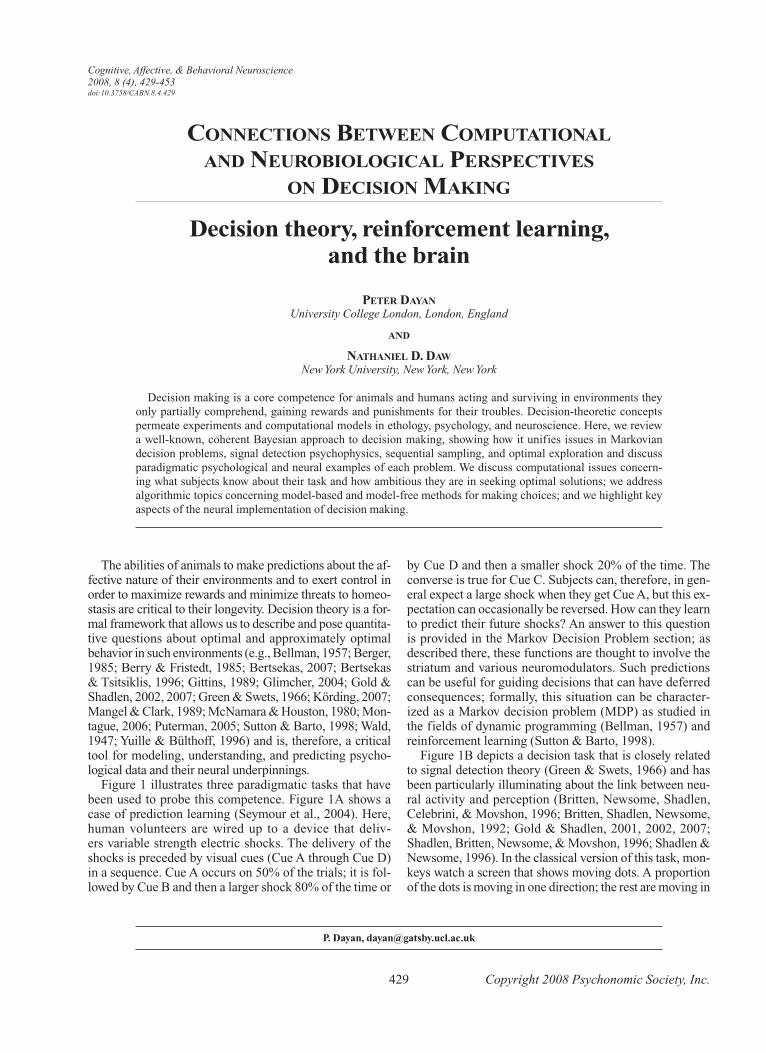
Figure 1 illustrates three paradigmatic tasks that have been used to probe this competence. Figure 1A shows a case of prediction learning (Seymour et al., 2004). Here, human volunteers are wired up to a device that deliv­ers variable strength electric shocks. The delivery of the shocks is preceded by visual cues (Cue A through Cue D) in a sequence. Cue A occurs on 50% of the trials; it is fol­lowed by Cue B and then a larger shock 80% of the time or

by Cue D and then a smaller shock 20% of the time. The converse is true for Cue C. Subjects can, therefore, in gen­eral expect a large shock when they get Cue A, but this ex­pectation can occasionally be reversed. How can they learn to predict their future shocks? An answer to this question is provided in the Markov Decision Problem section; as described there, these functions are thought to involve the striatum and various neuromodulators. Such predictions can be useful for guiding decisions that can have deferred consequences; formally, this situation can be character­ized as a Markov decision problem (MDP) as studied in the fields of dynamic programming (Bellman, 1957) and reinforcement learning (Sutton & Barto, 1998).

Figure 1B depicts a decision task that is closely related to signal detection theory (Green & Swets, 1966) and has been particularly illuminating about the link between neu­ral activity and percep tion (Britten, Newsome, Shadlen, Celebrini, & Movshon, 1996; Britten, Shadlen, Newsome, & Movshon, 1992; Gold & Shadlen, 2001, 2002, 2007; Shadlen, Britten, Newsome, & Movshon, 1996; Shadlen & Newsome, 1996). In the classical version of this task, mon­keys watch a screen that shows moving dots. A proportion of the dots is moving in one direction; the rest are moving in

429 Copyright 2008 Psychonomic Society, Inc.

ConneCtions Between Computational and neuroBiologiCal perspeCtives

on deCision making

Decision theory, reinforcement learning, and the brain

peter dayanUniversity College London, London, England

and

nathaniel d. dawNew York University, New York, New York

Decision making is a core competence for animals and humans acting and surviving in environments they only partially comprehend, gaining rewards and punishments for their troubles. Decision­theoretic concepts permeate experiments and computational models in ethology, psychology, and neuroscience. Here, we review a well­known, coherent Bayesian approach to decision making, showing how it unifies issues in Markovian decision problems, signal detection psychophysics, sequential sampling, and optimal exploration and discuss paradigmatic psychological and neural examples of each problem. We discuss computational issues concern­ing what subjects know about their task and how ambitious they are in seeking opti mal solutions; we address algorithmic topics concerning model­based and model­free methods for making choices; and we highlight key aspects of the neural implementation of decision making.

Cognitive, Affective, & Behavioral Neuroscience2008, 8 (4), 429-453doi:10.3758/CABN.8.4.429

P. Dayan, dayan@gatsby.ucl.ac.uk

430 Dayan anD Daw

of the method for solving the problems, and discuss these particular cases and their near relatives in some detail. A wealth of problems and solu tions that has arisen in different areas of psychology and neurobiology is thereby integrated, and common solution mechanisms are identified. In particu­lar, viewing these problems as differ ent specializations of a common task involving both sensory inference and learning

random directions. The monkeys have to report the coher­ent direction by making a suitable eye move ment. By vary­ing the fraction of the dots that moves coherently (called the coherence), the task can be made easier or harder. The visual system of the monkey reports evidence about the direc tion of motion; how should the subject use this infor­mation to make a decision? In some versions of the task, the monkey can also choose when to emit its response; how can it decide whether to respond or to continue collecting in­formation? These topics are addressed in the Signal Detec­tion Theory and Temporal State Uncertainty sections, along with the roles of two visual cortical areas (MT and lateral intraparietal area [LIP]). The simpler version can be seen as a standard signal detection theory task; the more complex one has been analyzed by Gold and Shad len (2001, 2007) as an optimal­stopping problem. This, in turn, is a form of partially observ able MDP (POMDP) related to the sequen­tial probability ratio test (SPRT; Ratcliff & Rouder, 1998; Shadlen, Hanks, Churchland, Kiani, & Yang, 2007; Smith & Ratcliff, 2004; Wald, 1947).

Finally, Figure 1C shows a further decision­theoretic wrinkle in the form of an experiment on the trade­off between exploration and exploitation (Daw, O’Doherty, Dayan, Seymour, & Dolan, 2006). Here, human subjects have to choose between four one­armed bandit machines whose payoffs are changing over time (shown by the curves inside each). The subjects can find out about the current value of a machine only by choosing it and, so, have to balance picking the machine that is currently believed best against choosing a machine that has not recently been sampled, in case its value has increased. Problems of this sort are surprisingly computationally intractable (Berry & Fristedt, 1985; Gittins, 1989); the section of the present article on Exploration and Exploitation discusses the issues and approximate solutions, including one that, evidence suggests, implicates the fronto­polar cortex.

Despite the apparent differences between these tasks, they actually share some deep underlying commonalities. In this review, we provide a straightforward formal framework that shows the links, give a computationally minded view

A B C

Cue A Cue B Highpain

Cue C Cue D Lowpain

Saccade

Motion

Targets

Fixation RF

Reaction Time

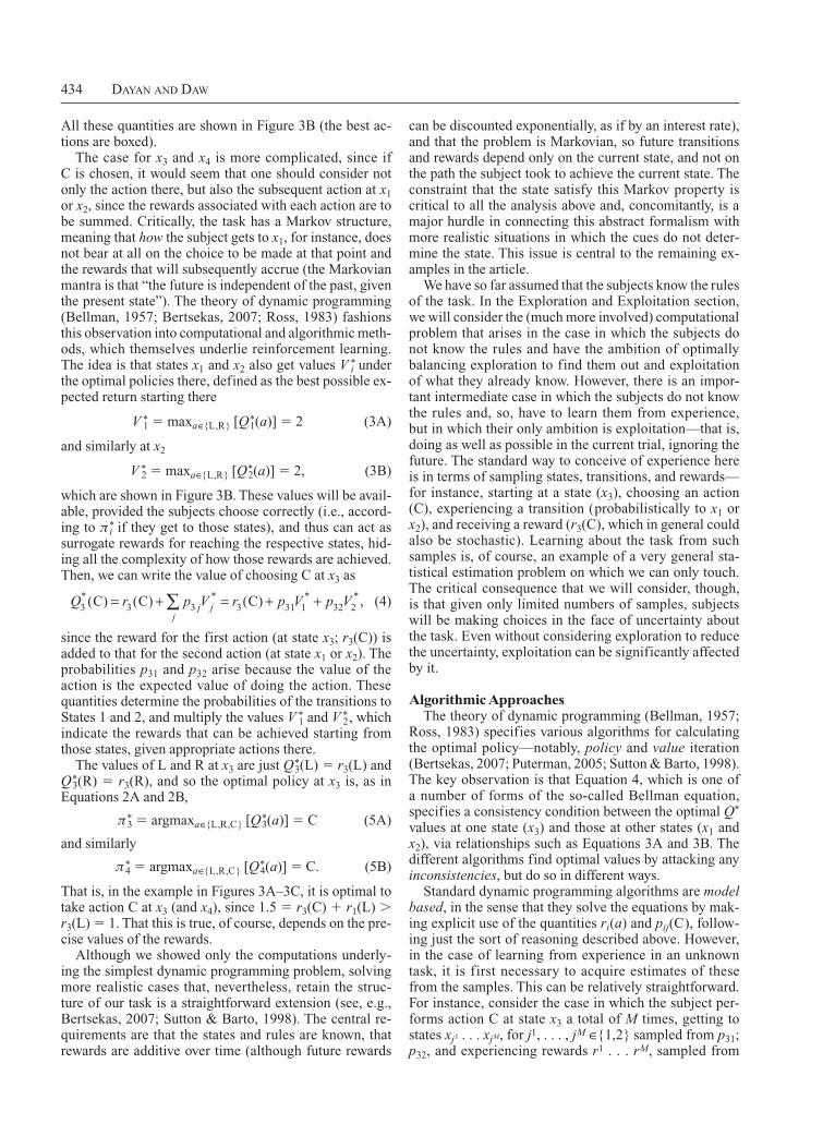
Figure 1. Paradigmatic tasks. (A) Subjects can predict the magnitude of future pain from partially informa-tive visual cues that follow a Markov chain (Seymour et al., 2004; see the Markov Decision Problem section). (B) Monkeys have to report the direction of predominant motion in a random-dot kinematogram by making an eye movement (Britten, Shadlen, Newsome, & Movshon, 1992); see the Signal Detection Theory section. In some experiments, the monkeys have the additional choice of whether to act or collect more information (Gold & Shad-len, 2007); see the Temporal State Uncertainty section. (C) Subjects have to choose between four evolving, noisy bandit machines (whose payments are shown in the insets) and, so, must balance exploration and exploitation (Daw, O’Doherty, Dayan, Seymour, & Dolan, 2006); see the Exploration and Exploitation section.

c1

r1(L) r1(R) r2(L)

R

R

L

L

CC

L

L

c2x1

p31 p32r3(C)

r3(L) r3(R) r4(L)

r2(R)

R

R

x2

r4(R)

c3 c4x3 x4

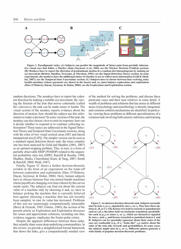
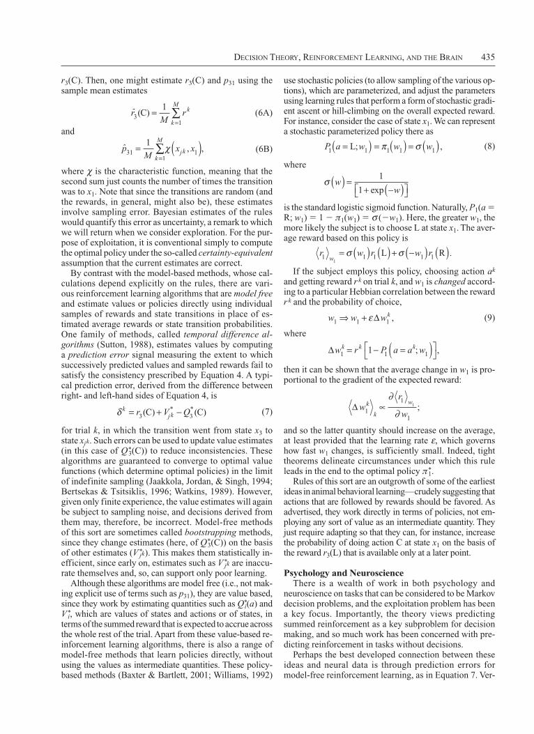
Figure 2. An abstract decision-theoretic task. Subjects normally start in state x3 or x4, signaled by cues c3 or c4. They have three op-tions (L, R, or C): The former two lead to rewards or punishments such as r3(L); the latter lead via stochastic transitions (probabili-ties such as p31) to states x1 or x2, which are themselves signaled by cues c1 and c2, and license rewarded or punished choices L and R. Subjects can be (partially) ignorant about their states if the cues are confusable (e.g., if x3 “looks like” x4), and/or about the rules of the task (the rewards and probabilities). In some cases, the subjects might start in x1 or x2. Different options generate a wide family of popular decision-theoretic problems.

Decision Theory, reinforcemenT Learning, anD The Brain 431

In terms of knowledge, the subjects might be ignorant of their precise state in the problem (i.e., which xi they cur­rently occupy), and/or the rules of the task (i.e., the transi­tion probabilities and rewards contingent on particular ac­tions in states). If they know both in the standard version of the task, which requires L at x3 and x1 and R at x4 and x2, with C being costly, and they know that they are at x3, say, they should choose L. However, if they know the rules and know that they are at either x3 or x4, but do not know which for sure (perhaps because the cues c3 and c4 are similar or identical), it might be worth the cost of choosing C in order to collect information from c1 and c2 (if these are more dis­tinct), the better to work out which action is then best.

The problems of balancing such costs and benefits get much harder if the subjects might not even completely know the rules of the task. This is necessarily the case at the outset of animal experi ments and is also more persis­tently true when, as is common in experiments, the rules are changed over time. In these cases, subjects will have to learn the rules from experience. However, experience will normally only partly specify the rules, leaving some ignorance and uncertainty, and it will often be important to take proper account of this.

Second, in terms of their ambition, the subjects might have the modest goal of exploitation—that is, trying to make the reward for the current trial as valuable as pos­sible, given whatever they cur rently know about the task. In the case in which the subjects start at x3 or x4, this in­volves comparing rewards available for the immediate choice of L or R with the integrated cost of C and the subse quent reward from L or R at x1 or x2. How to trade off immediate and deferred reward optimally depends on subjects’ preferences with respect to temporal discounting (e.g., Ainslie, 2001; Kable & Glimcher, 2007; McClure, Laibson, Loewenstein, & Cohen, 2004).

More ambitious subjects might seek to combine explo­ration and exploitation. That is, they might look to make every single choice correctly in the light of the fact that not only might it lead to a good outcome on this trial, but also it could provide information that will lead the subject to be more proficient at getting better outcomes in the future. This goal—choosing so as to maximize the inte­grated rewards obtained over many trials throughout the course of learning, trading off the immediate benefits of exploitation and the deferred benefits of exploration—is sometimes called lifetime optimality. Again, how these are balanced depends on temporal discounting.

Note that these two computational dimensions are not wholly independent; for instance, given complete knowl­edge of rules and state, exploration is moot.

Algorithmic IssuesDifferent points along the combined computational di­

mensions lead to a wide variety of different problems. Some of these are formally tractable—that is, have algorithms that require only moderate amounts of memory space or time to compute optimal solutions. Other points, particularly those involving incomplete knowledge or lifetime optimality, are much more challenging and typically require approxima­tions, even for nonneurobiological systems.

components gives strong clues as to how sensory systems and computational mechanisms involved in the sig nal detec­tion tasks—such as areas MT and LIP—are likely to interact with the basal ganglia and neuromodulatory systems that are implicated in the reinforcement learning tasks.

We tie the problems together by inventing a new, slightly more abstract assignment (shown in Figure 2). Particular specializations of this abstraction are then isomorphic to the tasks associated with Figure 1. The case of Figure 2 is an apparently simple maze­like choice task that we might present to animal or human subjects, who have to make decisions (here, choices between actions L, R, and C) in order to optimize their outcomes (r). Optimal choices in­volve balancing current and future rewards and costs and handling different forms of uncertainty about the rules of the task and the state within it.

Two critical dimensions that emerge from a consider­ation of Figure 2 concern what the subjects know and what they are trying to accomplish. The prediction task shown in Figure 1A arises when subjects are ignorant of the rules of the task but know their state or situation within it. Con­versely, the psy chophysical discrimination tasks shown in Figure 1B originate in a case in which subjects know the rules of the task but are only incompletely certain about the state. The exploration/exploitation trade­off shown in Figure 1C can be seen as combining both of these in a case in which subjects are ambitious about behaving optimally in the face of whatever uncertainty they have. Critically, through the medium of the task shown in Figure 2, all these problems can be characterized as requiring common computations. Realizing the computations leads to algo­rithmic issues having to do with different ways in which in formation from past and present trials can be accumu­lated and, thence, to implementational issues in terms of the neural structures involved in the solutions.

FOUNDATIONAL ISSUES

The task shown in Figure 2 involves only four choice points or states (x1, x2, x3, and x4) signaled, perhaps imper­fectly (i.e., leaving some uncertainty, in a way we will for­mulate precisely later), by cues (c1, c2, c3, and c4). Three actions are possible (L, R, and C) at the states, and it is the choices between these that the subjects must make. The choices lead to rewards or punishments (with values or utilities r, which depend on the states and actions), and/or to transitions from one state to the next (x3 to x1 or x2, etc.). We consider that single trials end when an actual outcome is achieved; the subjects then start again. In general, sub­jects’ choices may be only probabilistically related to the outcomes. In the standard case for this review, we will have the rewards being biggest for L at x3 and x1 and for R at x4 and x2, with C being costly. The subjects may not know these payoffs at the outset.

Computational IssuesAs has been mentioned, there are two main dimensions

defining the problem for the subjects: one having to do with what they are assumed to know about the task, the other defining the nature of their ambition.

432 Dayan anD Daw

and refined state abstraction on which these theories rely and the rich, multifarious, and ambiguous sensory world actually facing an organism.

Conversely, model­based methods for state estimation from noisy sensory input have been extensively investi­gated in a rather different set of psychophysical tasks (Brit­ten et al., 1996; Britten et al., 1992; Gold & Shad len, 2007; Parker & Newsome, 1998; Platt & Glimcher, 1999), exem­plified by Figure 1B, focusing on the mapping of input in­formation coded in sensory regions into decision­theoretic quantities coded in more motor­associated regions of the cortex. However, this work has generally confined itself to fairly rudimentary and limited forms of learning.

The aim of the remainder of this article is to situate both learning and state estimation mechanisms in a single framework.

We will use the examples shown in Figure 1, rendered in the abstract forms shown in Figure 2, to illustrate the key gen eral principles established above. The examples cover neural reinforcement learning (Montague et al., 1996; Schultz et al., 1997), Bayesian psychophysics (Brit­ten et al., 1992; Shadlen & New some, 1996), information gathering and optimal stopping (Gold & Shadlen, 2001, 2007), and the exploration/exploitation trade­off (Daw, O’Doherty, et al., 2006). The first example develops basic reinforce ment learning methods for tasks in which the state is known; the rest exemplify how these can be ex­tended, with belief states as the formal replacement for uncertain true states.

In each section, we first will describe the formal com­putational notions and ideas, then the relevant algorithmic methods associated with the computations, and finally the psychological and neuro biological tasks and mechanisms that are implicated.

ThE MARkOv DECISION PROBLEM

The central problem in the prediction task shown in Fig­ure 1A is that until the subject observes Cue A or C at the start of a trial, he or she does not know whether he or she will receive a shock at the end of the trial; the cue makes the outcome more predictable. In Markov problems—that is, domains in which only the current state matters, and not the previous history—there turns out to be a computation­ally precise way of defining the goal for predicting future reinforcers. When a choice of actions is available, the goal also provides a formalization of optimal selection. There is also a variety of algorithmic methods for acquiring pre­dictions and using the predictions for control.

The Computational ProblemConsider the case shown in Figure 3A, in which the cues

unambiguously identify the state (c1 for x1, and so on). We will first consider decision making when the rules are given and then move onto the standard reinforcement learning problem in which the rules of the task are unknown and the subject must discover how best to behave by trial and error.

Given the rules, the task for the subject is simply to work out the best policy, p*

i (the asterisk identifying it as being best), which specifies an assignment of an action

Algorithms differ in how they draw on experience to es­timate quantities relevant to the deci sion and in how they render these into choices. The most important algorithmic dimension is that distinguishing model-based and model-free methods (Sutton & Barto, 1998). Crudely speaking, model­based methods make explicit use of the actual, or learned, rules of the task to make choices. Importantly, even when the rules are fully known, it takes some compu­tation to derive the optimal decision for a particular state from these more basic quantities.

Model­free methods eschew the rules of the task and, in­stead, use and/or learn putatively simpler quantities that are sufficient to permit optimal choices. For instance, in Fig­ure 2, given complete knowledge of the state, it clearly is enough just to know four letters—namely, the best choices at x1 . . . x4. This is an example of a policy. Obtaining it in the face of ignorance of the rules lies at the heart of reinforce­ment learning methods. Policies can be learned directly or can be derived from other informa tion, such as the expected future utilities (values) that will accrue from different ac­tions or states. Policies can also be derived (in model­based methods) from the rules of the task. Indeed, one of the most important products of the field of reinforcement learning (Sutton & Barto, 1998) is a range of model­free algorithms for solving the exploitation problem.

When the observations or cues do not precisely pin down the state, a policy mapping states to actions is obvi­ously of little use. Given a model of the rules, including those relating states such as x3 to cues such as c3, the be­liefs about the current state (called the belief state) can be calculated on the basis of the observations. The belief state can then, in a formal sense, stand in for the true state, so the policy becomes a function of this instead. This sub­stitution of belief state for state is a recurring theme in the solution to the tasks discussed below.

Implementational IssuesIt has long been suggested that there is a rather direct

mapping of model­free reinforcement learn ing algorithms onto the brain, with the neuromodulator dopamine serving as a teaching signal to train values or policies by control­ling synaptic plasticity at targets such as the ventral and dorso lateral striatum (Barto, 1995; Daw, Niv, & Dayan, 2005; Friston, Tononi, Reeke, Sporns, & Edelman, 1994; Joel, Niv, & Ruppin, 2002; Montague, Dayan, & Sej­nowski, 1996; Schultz, Dayan, & Montague, 1997; Suri & Schultz, 1998; Wickens, 1990). For aversive outcomes such as the shocks shown in Figure 1A, there is much less evidence about the overall neural substrate. More recently, it has been suggested that the brain also employs model­based methods for planning under un certainty about the rules, in a different set of circuits involving the prefrontal cortex and the dorsomedial striatum (Balleine, Delgado, & Hikosaka, 2007; Daw et al., 2005; Dickinson & Bal­leine, 2002; Everitt & Robbins, 2005).

Most of this work has focused on rule, value, or policy learning, ignoring the issue of state un certainty; indeed, arguably, the primary obstacle toward employing either the model­based or the model­free methods in a real­world context is the gulf between the highly constrained

Decision Theory, reinforcemenT Learning, anD The Brain 433

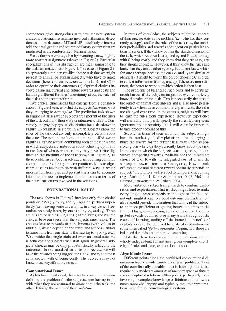
the value of each action Q*1(a), defined as the expected

return for performing that action, is

Q*1(a) 5 r1(a), (1)

and a best action (i.e., one that maximizes this expected return) is

p*1 5 argmaxa∈{L,R} [Q*

1(a)] 5 L, (2A)

and similarly

p*2 5 argmaxa∈{L,R} [Q*

2(a)] 5 R. (2B)

a ∈{L, R, C} to each state xi. The probabilities pij 5 pij(C) indicate the probabilities of going from state xi to xj under action C, whose cost is ri(C); actions L and R have de­terministic consequences. Exactly how the “best” policy is defined depends on the particular goal. For now, we will assume that the rewards and costs earned across each whole single trial are simply summed, and it is this sum that has to be predicted and optimized.

First, consider the case in which the goal is exploitation within a single trial, to maximize the average, or expected, reward. If we consider state x1, the task is straightforward;

c1

r1(L) = 2 r1(R) = 0 r2(L) = 0

R

R

L

L

CC

L

L

c2x1

p31 = .9 p32 = .1

r3(C) = –0.5

r3(L) = 1 r3(R) = 0 r4(L) = 0

r2(R) = 2

R

R

x2

r4(R) = 1

c3 c4x3 x4

c1

V 1* = 2

c2

V 2* = 2

RL L

x1

p31 = .9 p32 = .1

Q3*(C) = 1.5

Q3*(L) = 1 Q3

*(R) = 0 Q4*(L) = 0

R

x2

c1

V 1* = 2

Q1*(L) = 2 Q1

*(R) = 0

R

x1

Q4*(R) = 1

c3 c4x3 x4

π1* = L L

c2

V 2* = 2

Q2*(L) = 0 Q2

*(R) = 2

x2

π2* = R

π3* = C π4

* = C

A

B C

Figure 3. Markov decision problem (MDP). (A) The version of the basic task rendered as a simple MDP. Each state xi has a distinct cue ci, and the rewards and transition probabilities are as shown (the case for C at x4 is symmetric with respect to x3). The solution to MDP involves optimal state-action values Q*

i(a), state values V*i, and thence the optimal policy p*

i (shown in the boxes) first for states x1 and x2 (B), and then for x3 and x4 (C). The calculation for x3 and x4 depends only on V*

1 and V*2 and not on the manner by which the

reward from x1 or x2 is achieved.

434 Dayan anD Daw

can be discounted exponentially, as if by an interest rate), and that the problem is Markovian, so future transitions and rewards depend only on the current state, and not on the path the subject took to achieve the current state. The constraint that the state satisfy this Markov property is critical to all the analysis above and, concomitantly, is a major hurdle in con necting this abstract formalism with more realistic situations in which the cues do not deter­mine the state. This issue is central to the remaining ex­amples in the article.

We have so far assumed that the subjects know the rules of the task. In the Exploration and Exploitation section, we will consider the (much more involved) computational problem that arises in the case in which the subjects do not know the rules and have the ambition of optimally balancing exploration to find them out and exploitation of what they already know. However, there is an impor­tant intermediate case in which the subjects do not know the rules and, so, have to learn them from experience, but in which their only ambition is exploitation—that is, doing as well as possible in the current trial, ignoring the future. The standard way to conceive of experience here is in terms of sampling states, transitions, and rewards—for instance, starting at a state (x3), choosing an action (C), experiencing a transition (probabilistically to x1 or x2), and receiving a reward (r3(C), which in general could also be stochastic). Learning about the task from such samples is, of course, an example of a very general sta­tistical estimation problem on which we can only touch. The critical consequence that we will consider, though, is that given only limited numbers of samples, subjects will be making choices in the face of uncertainty about the task. Even without considering exploration to reduce the uncertainty, exploitation can be significantly affected by it.

Algorithmic ApproachesThe theory of dynamic programming (Bellman, 1957;

Ross, 1983) specifies various algorithms for calculating the optimal policy—notably, policy and value iteration (Bertsekas, 2007; Puterman, 2005; Sutton & Barto, 1998). The key observation is that Equation 4, which is one of a number of forms of the so­called Bellman equation, specifies a consistency condition between the optimal Q* values at one state (x3) and those at other states (x1 and x2), via relationships such as Equations 3A and 3B. The different algorithms find optimal values by attacking any inconsistencies, but do so in different ways.

Standard dynamic programming algorithms are model based, in the sense that they solve the equa tions by mak­ing explicit use of the quantities ri(a) and pij(C), follow­ing just the sort of reasoning described above. However, in the case of learning from experience in an unknown task, it is first necessary to acquire estimates of these from the samples. This can be relatively straightforward. For instance, consider the case in which the subject per­forms action C at state x3 a total of M times, getting to states xj1 . . . xj M, for j1, . . . , jM ∈{1,2} sampled from p31; p32, and experiencing rewards r1 . . . rM, sampled from

All these quantities are shown in Figure 3B (the best ac­tions are boxed).

The case for x3 and x4 is more complicated, since if C is chosen, it would seem that one should consider not only the action there, but also the subsequent action at x1 or x2, since the rewards associated with each action are to be summed. Critically, the task has a Markov structure, meaning that how the subject gets to x1, for instance, does not bear at all on the choice to be made at that point and the rewards that will subsequently accrue (the Markovian mantra is that “the future is independent of the past, given the present state”). The theory of dynamic programming (Bellman, 1957; Bertsekas, 2007; Ross, 1983) fashions this observation into computational and algorithmic meth­ods, which themselves underlie reinforcement learning. The idea is that states x1 and x2 also get values V *

i under the optimal policies there, defined as the best possible ex­pected return starting there

V *1 5 maxa∈{L,R} [Q*

1(a)] 5 2 (3A)

and similarly at x2

V *2 5 maxa∈{L,R} [Q*

2(a)] 5 2, (3B)

which are shown in Figure 3B. These values will be avail­able, provided the subjects choose correctly (i.e., accord­ing to p*

i if they get to those states), and thus can act as surrogate rewards for reaching the respective states, hid­ing all the complexity of how those rewards are achieved. Then, we can write the value of choosing C at x3 as

Q r p V r p V p Vj jj

3 3 3 3 31 1 32 2* * * *( ) ( ) ( ) ,C C C= + = + +∑ (4)

since the reward for the first action (at state x3; r3(C)) is added to that for the second action (at state x1 or x2). The probabilities p31 and p32 arise because the value of the action is the expected value of doing the action. These quantities determine the probabilities of the transitions to States 1 and 2, and multiply the values V *

1 and V *2, which

indicate the rewards that can be achieved starting from those states, given appropriate actions there.

The values of L and R at x3 are just Q*3(L) 5 r3(L) and

Q*3(R) 5 r3(R), and so the optimal policy at x3 is, as in

Equations 2A and 2B,

p*3 5 argmaxa∈{L,R,C} [Q*

3(a)] 5 C (5A)

and similarly

p*4 5 argmaxa∈{L,R,C} [Q*

4(a)] 5 C. (5B)

That is, in the example in Figures 3A–3C, it is optimal to take action C at x3 (and x4), since 1.5 5 r3(C) 1 r1(L) . r3(L) 5 1. That this is true, of course, depends on the pre­cise values of the rewards.

Although we showed only the computations underly­ing the simplest dynamic programming problem, solving more realistic cases that, nevertheless, retain the struc­ture of our task is a straightforward extension (see, e.g., Bertsekas, 2007; Sutton & Barto, 1998). The cen tral re­quirements are that the states and rules are known, that rewards are additive over time (although future rewards

Decision Theory, reinforcemenT Learning, anD The Brain 435

use stochastic policies (to allow sampling of the various op­tions), which are parameterized, and adjust the parameters using learning rules that perform a form of stochastic gradi­ent ascent or hill­climbing on the over all expected reward. For instance, consider the case of state x1. We can represent a stochastic parameterized policy there as

where

P a w w w

ww

1 1 1 1 1

1

1

=( ) = ( ) = ( )

( ) =+ −( )

L;

exp

π σ

σ

,

(8)

is the standard logistic sigmoid function. Naturally, P1(a 5 R; w1) 5 1 2 p1(w1) 5 σ (2w1). Here, the greater w1, the more likely the subject is to choose L at state x1. The aver­age reward based on this policy is

r w r w rw1 1 1 1 1

1

= ( ) ( ) + −( ) ( )σ σL R .

If the subject employs this policy, choosing action ak and getting reward rk on trial k, and w1 is changed accord­ing to a particular Hebbian correlation between the reward rk and the probability of choice,

where

w w w

w r P a a w

k

k k k

1 1 1

1 1 11

⇒ + ∆

∆ = − =( )

ε ,

; ,

(9)

then it can be shown that the average change in w1 is pro­portional to the gradient of the expected reward:

∆ ∝wr

wk

k

w

1

1

1

1

∂

∂;

and so the latter quantity should increase on the average, at least provided that the learning rate ε, which governs how fast w1 changes, is sufficiently small. Indeed, tight theorems delineate circumstances under which this rule leads in the end to the optimal policy p*

1.Rules of this sort are an outgrowth of some of the earliest

ideas in animal behavioral learning—crudely suggesting that actions that are followed by rewards should be favored. As advertised, they work directly in terms of policies, not em­ploying any sort of value as an intermediate quan tity. They just require adapting so that they can, for instance, increase the probability of doing action C at state x1 on the basis of the reward r3(L) that is available only at a later point.

Psychology and NeuroscienceThere is a wealth of work in both psychology and

neuroscience on tasks that can be considered to be Markov decision problems, and the exploitation problem has been a key focus. Importantly, the theory views predicting summed reinforcement as a key subproblem for decision making, and so much work has been concerned with pre­dicting reinforcement in tasks without decisions.

Perhaps the best developed connection between these ideas and neural data is through prediction errors for model­free reinforcement learning, as in Equation 7. Ver­

r3(C). Then, one might estimate r3(C) and p31 using the sample mean estimates

r̂M

rk

k

M

31

1(C) =

=∑ (6A)

and

p̂M

x xjkk

M

31 11

1= ( )=

∑c , , (6B)

where c is the characteristic function, meaning that the second sum just counts the number of times the transition was to x1. Note that since the transitions are random (and the rewards, in general, might also be), these estimates involve sampling error. Bayesian estimates of the rules would quantify this error as uncertainty, a remark to which we will return when we consider exploration. For the pur­pose of exploitation, it is conventional simply to compute the optimal policy under the so­called certainty-equivalent assumption that the current estimates are correct.

By contrast with the model­based methods, whose cal­culations depend explicitly on the rules, there are vari­ous reinforcement learning algorithms that are model free and estimate values or policies directly using individual samples of rewards and state transitions in place of es­timated average rewards or state transition probabilities. One family of methods, called temporal difference al-gorithms (Sutton, 1988), estimates values by computing a prediction error signal measuring the extent to which successively predicted values and sampled rewards fail to satisfy the consistency prescribed by Equation 4. A typi­cal prediction error, derived from the difference between right­ and left­hand sides of Equation 4, is

δ kjkr V Q= + −3 3(C) (C)* * (7)

for trial k, in which the transition went from state x3 to state xj k. Such errors can be used to update value estimates (in this case of Q*

3(C)) to reduce inconsistencies. These algorithms are guaranteed to converge to optimal value functions (which determine optimal policies) in the limit of indefinite sampling (Jaakkola, Jordan, & Singh, 1994; Bertsekas & Tsitsiklis, 1996; Watkins, 1989). However, given only finite experience, the value estimates will again be subject to sampling noise, and decisions derived from them may, therefore, be incorrect. Model­free methods of this sort are sometimes called bootstrapping methods, since they change estimates (here, of Q*

3(C)) on the basis of other estimates (V*

j k). This makes them statistically in­efficient, since early on, estimates such as V*

j k are inaccu­rate themselves and, so, can support only poor learning.

Although these algorithms are model free (i.e., not mak­ing explicit use of terms such as p31), they are value based, since they work by estimating quantities such as Q*

i(a) and V*

i, which are values of states and actions or of states, in terms of the summed reward that is expected to accrue across the whole rest of the trial. Apart from these value­based re­inforcement learning algorithms, there is also a range of model­free methods that learn policies directly, without using the values as intermediate quanti ties. These policy­based methods (Baxter & Bartlett, 2001; Williams, 1992)

436 Dayan anD Daw

report quantities akin to the temporal difference predic­tion error in Equation 7. This comes on top of a huge body of results on the involvement of dopamine and its striatal projection in appetitive learning and appetitively motivated choice behavior (for some recent highlights, see Costa, 2007; Hyman, Malenka, & Nestler, 2006; Joel et al., 2002; Wickens, Horvitz, Costa, & Killcross, 2007). The pro­posal that this operates according to the rules of reinforce­ment learning (Balleine et al., 2007; Barto, 1995; Daw & Doya, 2006; Haruno et al., 2004; Joel et al., 2002; Mon­tague et al., 1996; O’Doherty, Dayan, Friston, Critchley, & Dolan, 2003; O’Doherty et al., 2004; Schultz et al., 1997; Suri & Schultz, 1998), in a way that ties together the at least equally extensive data on the psychology of instrumental choice with these neural data, has extensive, although not universal, support (e.g., Berridge, 2007; Redgrave, Gurney, & Reynolds, 2008).

However, behaviorally sophisticated experiments (re­viewed in Balleine et al., 2007; Dickinson & Balleine, 2002) show that this is nothing like the whole story. These experiments study the effects of changing the desirabil­ity of rewards just before animals are allowed to exploit their learning. Model­based methods of control can use their explicit representation of the rules to modify their choices immediately in the light of such changes, whereas model­free methods, whose values change only through prediction errors (such as Equation 7), require further ex­perience to do so (Daw et al., 2005). There is evidence for both sorts of control, with model­based choices (called goal-directed actions) dominating for abbreviated expe­rience, certain sorts of complex tasks, and actions close to final outcomes. Model­free choices (called habits) are evident after more exten sive experience, in simple tasks, and for actions further from outcomes. Furthermore, these two forms of control can be differentially suppressed by selective lesions of parts of the medial prefrontal cortex in rats (Killcross & Coutureau, 2003). Daw et al. (2005) argued that the trade­off between goal­directed actions and habits is computationally grounded in the differential uncertainties of model­based and model­free control in the light of limited sampling experience.

sions of these have long played an important role in theo­ries of behavioral conditioning—most famously, that of Rescorla and Wagner (1972). More recently, neural corre­lates of such error signals have been detected in a number of tasks and species.

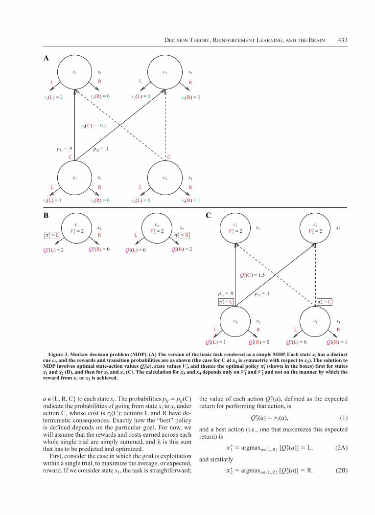
Consider the experiment shown in Figure 1A. The task was designed to induce higher order prediction errors—that is, those arising from changes in expectations about future reinforcement, rather than from the immediate receipt (or nonreceipt) of a primary reinforcer. Such er­rors are characteristic of the bootstrapping strategy of temporal­difference algorithms, which take the changes in expectations (e.g., the difference between V*

j k and Q*3 in

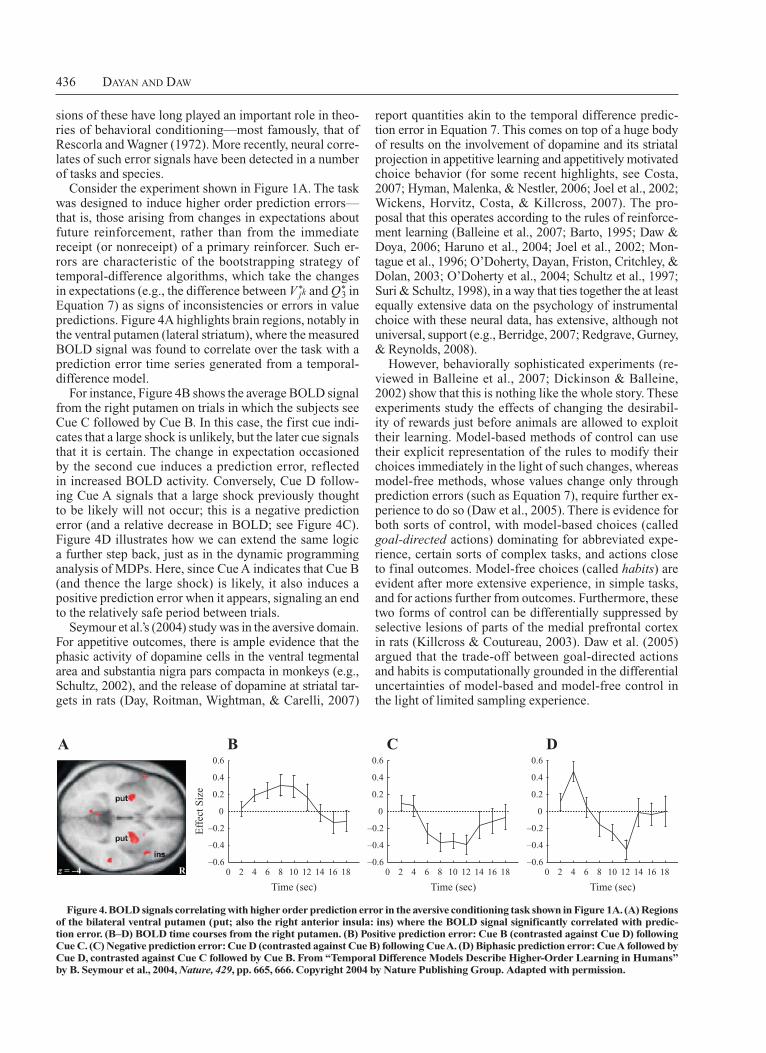
Equation 7) as signs of inconsistencies or errors in value predictions. Figure 4A highlights brain regions, notably in the ventral putamen (lateral striatum), where the measured BOLD signal was found to correlate over the task with a prediction error time series generated from a temporal­difference model.

For instance, Figure 4B shows the average BOLD signal from the right putamen on trials in which the subjects see Cue C followed by Cue B. In this case, the first cue indi­cates that a large shock is unlikely, but the later cue signals that it is certain. The change in expectation occasioned by the second cue induces a prediction error, reflected in increased BOLD activity. Conversely, Cue D follow­ing Cue A signals that a large shock previously thought to be likely will not occur; this is a negative prediction error (and a relative decrease in BOLD; see Figure 4C). Figure 4D illustrates how we can extend the same logic a further step back, just as in the dynamic programming analysis of MDPs. Here, since Cue A indicates that Cue B (and thence the large shock) is likely, it also induces a positive prediction error when it appears, signaling an end to the relatively safe period between trials.

Seymour et al.’s (2004) study was in the aversive domain. For appetitive outcomes, there is ample evidence that the phasic activity of dopamine cells in the ventral tegmental area and sub stantia nigra pars compacta in monkeys (e.g., Schultz, 2002), and the release of dopamine at striatal tar­gets in rats (Day, Roitman, Wightman, & Carelli, 2007)

A

z = –4 R

B0.6

0.4

0.2

0

–0.2

–0.4

–0.6

Eff

ect S

ize

0 2 4 6 8

Time (sec)

10 12 14 16 18

C0.6

0.4

0.2

0

–0.2

–0.4

–0.60 2 4 6 8

Time (sec)

10 12 14 16 18

D0.6

0.4

0.2

0

–0.2

–0.4

–0.60 2 4 6 8

Time (sec)

10 12 14 16 18

Figure 4. BOLD signals correlating with higher order prediction error in the aversive conditioning task shown in Figure 1A. (A) Regions of the bilateral ventral putamen (put; also the right anterior insula: ins) where the BOLD signal significantly correlated with predic-tion error. (B–D) BOLD time courses from the right putamen. (B) Positive prediction error: Cue B (contrasted against Cue D) following Cue C. (C) Negative prediction error: Cue D (contrasted against Cue B) following Cue A. (D) Biphasic prediction error: Cue A followed by Cue D, contrasted against Cue C followed by Cue B. From “Temporal Difference Models Describe higher-Order Learning in humans” by B. Seymour et al., 2004, Nature, 429, pp. 665, 666. Copyright 2004 by Nature Publishing Group. Adapted with permission.

Decision Theory, reinforcemenT Learning, anD The Brain 437

identity is at least partially hidden from the subjects. The subjective problem is illustrated in Figure 5B.

To formalize this task, it is necessary to specify the cou­pling between cues and states. The natural model of this involves the conditional distributions over the possible observations (the cues) given the states

p c c x x p c x1 1 1 1α α α= =( ) ≡ ( )| |

and

p c c x x p c x2 2 2 2α α α= =( ) ≡ ( )| | ,

which, in signal detection theory, are often assumed to be Gaussian, with means µ1 and µ2 (say, with µ1 . µ2) and variances σ 2

1 and σ 22. These distributions are shown

in miniature in Figures 5A and 5B.If the subject observes a particular cα, then, given these

distributions, what should it do? It needs a decision rule— a mapping, sometimes called a test—from its observation cα to a choice of action, L or R.

There are four possibilities for executing one of these actions at one of the two states. Standard signal detection theory privileges one of the actions (say, L) and, thus, one of the states (here, x1) and defines the four possibilities shown inside Table 1. Note that we could just as well have privileged R at x2. Signal detection theory stresses the trade­off between pairs of these outcomes. For instance, subjects could promiscuously choose L despite evidence from cα that x2 is more likely. This would reduce misses, at the expense of introducing more false alarms.

Under Bayesian decision theory, subjects should maxi­mize their expected reward, given the infor mation they have received. The first step is to use the observation cα to calculate the subjective belief state—that is, the posterior distribution over being in x1 or x2, given the data

P x x c P x cp c x P x

p cα α αα

α=( ) ≡ ( ) =

( ) ( )( )

=

1 11 1 1

1

1

| ||

++ ( )( )( )

1 2

1l c

P x

P xα

, (10)

Although more comprehensive, even this synthesis has an extremely limited scope. As was hinted above, the question of most relevance to the present review is how internally to create or infer a state space from just a boom­ing, baffling confusion of poorly segmentable cues. That is, how to extract the equivalent of x1 . . . x4, the underlying governors of the transitions and rewards, au tomatically from experience in an environment. The simplest versions of this issue are related to topics much more heavily stud­ied in sensory neuroscience and psychophysics, and we now will turn to these.

SIGNAL DETECTION ThEORy

The task shown in Figure 1B, in the version in which the subject cannot influence the length of time that the dots are shown, is one of sensory discrimination. Here, noisy and, therefore, unreliable evidence provided by motion­ processing areas in the visual system has to be used to make as good a decision as possible to maximize reward. It maps onto the basic task in the case in which the rules are known, but the ci inputs associated with the states are only partially informa­tive about the states (because of the effects of noise).

Variants of this task—notably, ones involving the detec­tion of a very weak sensory signal in the face of noise in the processing of input—are among the most intensively studied quantitative psy chophysical tasks; it was because of this that they came to be used to elucidate the neural under pinnings of decision making.

The Computational ProblemFigure 5A shows the variant of the basic abstract prob­

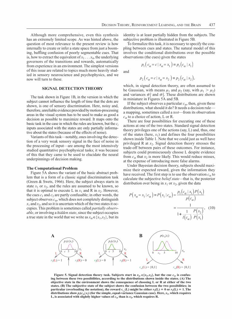
lem that is a form of a classic signal discrim ination task (Green & Swets, 1966). Here, the subject always starts in state x1 or x2, and the rules are assumed to be known, so that it is optimal to execute L in x1 and R in x2. However, the cues c1 and c2 are partly confusable; in other words, the subject observes cα, which does not completely distinguish x1 and x2, and so it is uncertain which of the two states it oc­cupies. This problem is sometimes called partially observ-able, or involving a hidden state, since the subject occupies a true state in the world that we write as xα ∈{x1,x2}, but its

0 5 10 0 5 100 5 10RLRL

cc

A B

RL

x1 x2

r1(L) = 1 r1(R) = 0 r2(L) = 0 r2(R) = 1

p1(c|x1) p2(c|x2)

xαcα

rc (L) = {0,1}α rc (R) = {0,1}α

p(c |xi)α

Figure 5. Signal detection theory task. Subjects start in xα  ∈{x1,x2}, but the cue cα is confus-ing between these two possibilities, according to the distributions shown inside the states. (A) The objective state in the environment shows the consequence of choosing L or R at either of the two states. (B) The subjective state of the subject shows the confusion between the two possibilities; in particular (overloading the notation), the reward rcα

(L) might be either r2(L) 5 0 or r1(L) 5 1. The distributions show pi(cα | xi) (for the simple, equal-variance Gaussian case). here, x1, which requires L, is associated with slightly higher values of cα than is x2, which requires R.

438 Dayan anD Daw

These value expressions are functions of the cue cα only through the belief state, which in this sense serves as a sufficient statistic for the cue in computing them. An­other way of saying this is that the belief state satisfies the Markov independence property on which our reinforce­ment learning analysis relies: Given it, the future reward expectation is independent of the past (here, the cue). By determining the value expectations for each action, the belief state plays the role of the state from the previous section, which is unobservable here.

Given these values, then, as in Equations 2A and 2B, we can choose an optimal policy,

πα αc a cQ* *=

∈argmax ( ) ,{L,R} a (14)

which, by direct calculation, turns out to just take the form of a threshold on the belief state or, equivalently, on the likelihood ratio l(cα), and can be written as

π

θ

θ

θα

α

α

α

c

l c

l c

l c

* =

( ) >

( ) <

× ( ) =

L if ,

R if ,

if ,

(15)

where 3 implies that either L or R should be chosen with equal probability.

Given our assumption that r1(L) . r1(R), the Bayes­optimal threshold θ B is determined by the rewards and priors according to

θB

R L

L R=

( ) − ( )( ) − ( )

( )( )

r r

r r

P x

P x2 2

1 1

2

1

, (16)

which comes from the point at which the values of the two actions are equal—that is,

Q Qc cα α

* * .L R( ) = ( )

where

l cp c x

p c xαα

α( ) =

( )( )

1 1

2 2

|

|, (11)

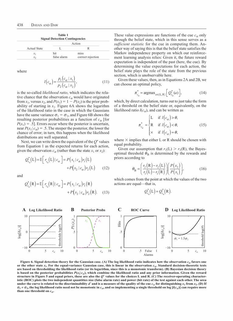
is the so­called likelihood ratio, which indicates the rela­tive chance that the observation cα would have originated from x1, versus x2, and P(x1) 5 1 2 P(x2) is the prior prob­ability of starting in x1. Figure 6A shows the logarithm of the likelihood ratio in the case in which the Gaussians have the same variance σ1 5 σ 2, and Figure 6B shows the resulting posterior probabilities as a function of cα [for P(x1) 5 .5]. Errors occur where the posterior is uncertain, near P(x1 | cα) 5 .5. The steeper the posterior, the lower the chance of error; in turn, this happens when the likelihood distributions are well separated.

Next, we can write down the equivalent of the Q* values from Equation 1 as the expected returns for each action, given the observation cα (rather than the state x1 or x2):

Q r c P x c r

P x c

c cα α α α

α

* L L L( ) = ( )

= ( ) ( )

+

| |

|

1 1

2(( ) ( )r2 L (12)

and

Q r c P x c r

P x c

c cα α α α

α

* R R R( ) = ( )

= ( ) ( )

+

| |

|

1 1

2(( ) ( )r2 R . (13)

0 .5 10

.5

1

C

Hit

s

ROC Curve

FalseAlarms

0 5 10−10

0

10

Log Likelihood RatioA

thre

shol

ds lo

g(θ)

0 5 100

.5

1

B Posterior Probs

x2

0 5 10−10

0

10

thre

shol

d lo

g(θ)

D Log Likelihood Ratio

x1

log[

l()]

c α

log[

l()]

c α

1 = 1.5 2σ σ

cαcα

P(x

i|)

c α

cα

Figure 6. Signal detection theory for the Gaussian case. (A) The log likelihood ratio indicates how the observation cα favors one or the other state xi. For the equal-variance Gaus sian case, this is linear in the observation cα. Standard decision-theoretic tests are based on thresholding the likelihood ratio (or its logarithm, since this is a mono tonic transform). (B) Bayesian decision theory is based on the posterior probabilities P(xi| cα), which combine the likelihood ratio and any prior information. Given the reward structure in Figure 5 and equal priors, these are also the Q* values for the choices L and R. (C) The receiver-operating character-istic (ROC) plots the two indepen dent quantities size (false alarm rate) and power (hit rate) of the test against each other. The area under the curve is related to the discriminability d ′

and is a measure of the quality of the cue cα for distinguishing x1 from x2. (D) If

σ1 ≠ σ 2, the log likelihood ratio need not be monotonic in cα, and so implementing a single threshold on log [l(cα)] can require more than one threshold on cα.

Table 1 Signal Detection Contingencies

Action

Actual State L R

x1 hit miss x2 false alarm correct rejection

Decision Theory, reinforcemenT Learning, anD The Brain 439

Similarly, the nature of the dependence of values such as Q*cα(L) on cα is determined by quantities to which model­free methods have no direct access. One general solu­tion is to use a flexible and general form for representing functions—for instance, writing

Q f c wc k kk

α α* .L L( ) = ( ) ( )∑ (18)

Here, fk(cα) are so­called basis functions of cα, and wk are parameters or weights whose settings determine the function. Depending on properties of Q*cα(L) such as smoothness, a close approximation to it can result from relatively small numbers of basis functions. Furthermore, the model­free methods described in the previous section can be used to learn the weights.

Similarly, model­free and value­free policy gradient methods can be used to learn weights that parameterize a policy p*cα directly. As is frequently the case, the policy ( just one, or sometimes more, thresholds) may be much simpler than the values (a form of sigmoid function), mak­ing it potentially easier to learn appropriate weights.

Psychology and NeuroscienceThe ample studies of human and animal psychophysics

provide rich proof that subjects are so phisticated signal detectors and deciders in the terms established above. Be­havior is exquisitely sensitive to alterations in the payoffs for different options (Stocker & Simoncelli, 2006) and changes in the observations (Körding & Wolpert, 2004); subjects even appear to have a good idea about the noise associated with their own sensations (Whiteley & Sahani, 2008) and actions (Trommershäuser, Landy, & Maloney, 2006; Trommershäuser, Maloney, & Landy, 2003a, 2003b) and can cope with even more sophisticated cases in which cues are two­dimensional (visual, cv

α; auditory, caα) and are

conditionally independent given the state (Battaglia, Ja­cobs, & Aslin, 2003; Ernst & Banks, 2002; Jacobs, 1999; Yuille & Bülthoff, 1996).

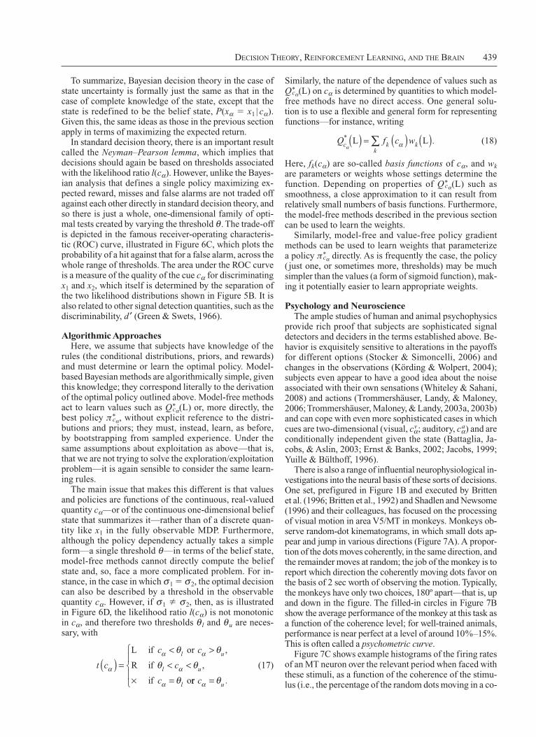
There is also a range of influential neurophysiological in­vestigations into the neural basis of these sorts of decisions. One set, prefigured in Figure 1B and executed by Britten et al. (1996; Britten et al., 1992) and Shadlen and Newsome (1996) and their colleagues, has focused on the processing of visual motion in area V5/MT in monkeys. Monkeys ob­serve random­dot kinematograms, in which small dots ap­pear and jump in various directions (Figure 7A). A propor­tion of the dots moves coherently, in the same direction, and the remainder moves at random; the job of the monkey is to report which direction the coherently moving dots favor on the basis of 2 sec worth of observing the motion. Typically, the monkeys have only two choices, 180º apart—that is, up and down in the figure. The filled­in circles in Figure 7B show the average performance of the monkey at this task as a function of the coherence level; for well­trained animals, performance is near perfect at a level of around 10%–15%. This is often called a psychometric curve.

Figure 7C shows example histograms of the firing rates of an MT neuron over the relevant period when faced with these stimuli, as a function of the coherence of the stimu­lus (i.e., the percentage of the random dots moving in a co­

To summarize, Bayesian decision theory in the case of state uncertainty is formally just the same as that in the case of complete knowledge of the state, except that the state is redefined to be the belief state, P(xα 5 x1 | cα). Given this, the same ideas as those in the previous section apply in terms of maximizing the expected return.

In standard decision theory, there is an important result called the Neyman–Pearson lemma, which implies that decisions should again be based on thresholds associated with the likelihood ratio l(cα). However, unlike the Bayes­ian analysis that defines a single policy maximizing ex­pected reward, misses and false alarms are not traded off against each other directly in standard decision theory, and so there is just a whole, one­dimensional family of opti­mal tests created by varying the threshold θ . The trade­off is depicted in the famous receiver­operating characteris­tic (ROC) curve, illustrated in Figure 6C, which plots the probability of a hit against that for a false alarm, across the whole range of thresholds. The area under the ROC curve is a measure of the quality of the cue cα for discriminating x1 and x2, which itself is determined by the separation of the two likelihood distributions shown in Figure 5B. It is also related to other signal detection quantities, such as the discriminability, d ′ (Green & Swets, 1966).

Algorithmic ApproachesHere, we assume that subjects have knowledge of the

rules (the conditional distributions, priors, and rewards) and must determine or learn the optimal policy. Model­based Bayesian methods are algorithmically simple, given this knowledge; they correspond literally to the derivation of the optimal policy outlined above. Model­free methods act to learn values such as Q*cα(L) or, more directly, the best policy p*cα, without explicit reference to the distri­butions and priors; they must, instead, learn, as before, by bootstrapping from sampled experience. Under the same assump tions about exploitation as above—that is, that we are not trying to solve the exploration/ exploitation problem—it is again sensible to consider the same learn­ing rules.

The main issue that makes this different is that values and policies are functions of the continuous, real­valued quantity cα—or of the continuous one­dimensional belief state that summarizes it—rather than of a discrete quan­tity like x1 in the fully observable MDP. Furthermore, although the policy dependency actually takes a simple form—a single threshold θ—in terms of the belief state, model­free methods cannot directly compute the belief state and, so, face a more complicated problem. For in­stance, in the case in which σ1 5 σ2, the optimal decision can also be described by a threshold in the observable quantity cα. However, if σ1 σ2, then, as is illustrated in Figure 6D, the likelihood ratio l(cα) is not monotonic in cα, and therefore two thresholds θ l and θu are neces­sary, with

t c

c c

c

c

l u

l u

l

α

α α

α

α

θ θθ θ

θ( ) =

< >

< <

× =

L if or ,

R if ,

if orr c uα θ=

.

(17)

440 Dayan anD Daw

The open circles in Figure 7B show the remarkable con­clusion of this part of the study. These report the result of the Bayesian decision­theoretic analysis described above, applied to the neural activity data of the neuron shown in Figure 7C. This so­called neurometric curve shows the probability that an ideal observer knowing the firing rate distributions of a single cell and making optimal decisions would get the answer right. This single cell would already support decisions of the same quality as those made by the

herent direction), for both of the two directions of motion. Mapping this onto our problem, the firing rate is the cue cα (from the perspective of neurons upstream), the state is the actual direction of motion of the stimulus, and the histograms in the figure are the conditional distributions p1(cα | x1) (hashed) and p2(cα | x2) (solid). It is apparent that these distributions are well separated for high­ coherence trials—thus supporting low error discrimination— and less well for low­coherence ones.

Figure 7. Britten, Shadlen, Newsome, and Movshon’s (1992) experiment on primate signal detection. (A) Ma-caque mon keys observed random-dot motion displays made from a mixture of coherent dots interpreted as mov-ing in one direction and incoherent dots moving at random. For these dots, the task was to tell whether the coherent collection was moving up or down. The percentage of coherently moving dots determined difficulty. (B) The filled points show the psychometric curve—that is, the discrimination performance as a function of the percentage of coherent dots. The open points show the quality of performance that would be optimally supported by a recorded neuron. (C) The graphs show histograms of the activity of a single MT neuron at three coherence levels over a 2-sec period, when the coherent motion was in its preferred direction (hashed) or opposite to this (solid). The larger the coherence, the larger the discriminability d ′, and the more easily an ideal observer counting the spikes just of this neuron would be able to judge the direction. From “The Analysis of visual Motion: A Comparison of Neuronal and Psychophysical Performance,” by k. h. Britten, M. N. Shadlen, W. T. Newsome, and J. A. Movshon, 1992, Journal of Neuroscience, 12, pp. 4746, 4751, 4752, copyright 1992 by the Society for Neuroscience, and Theoretical Neuro-science: Computational and Mathematical Modeling of Neural Systems (pp. 89, 90), by P. Dayan and L. F. Abbott, 2005, Cambridge, MA: MIT Press, copyright 2005 by MIT. Adapted with permission.

ACoherence:

CB

0 10 20 30 40 50 60

20

20

20

0

0

0

1.0

.8

.6

.4

1.00.1 10 100

Pro

babi

lity

Tri

al C

ount

Coherence 0.8%

Coherence 3.2%

Coherence 12.8%

Firing Rate (Hz)

NeurometricPsychometric

0% 50% 100%

Decision Theory, reinforcemenT Learning, anD The Brain 441

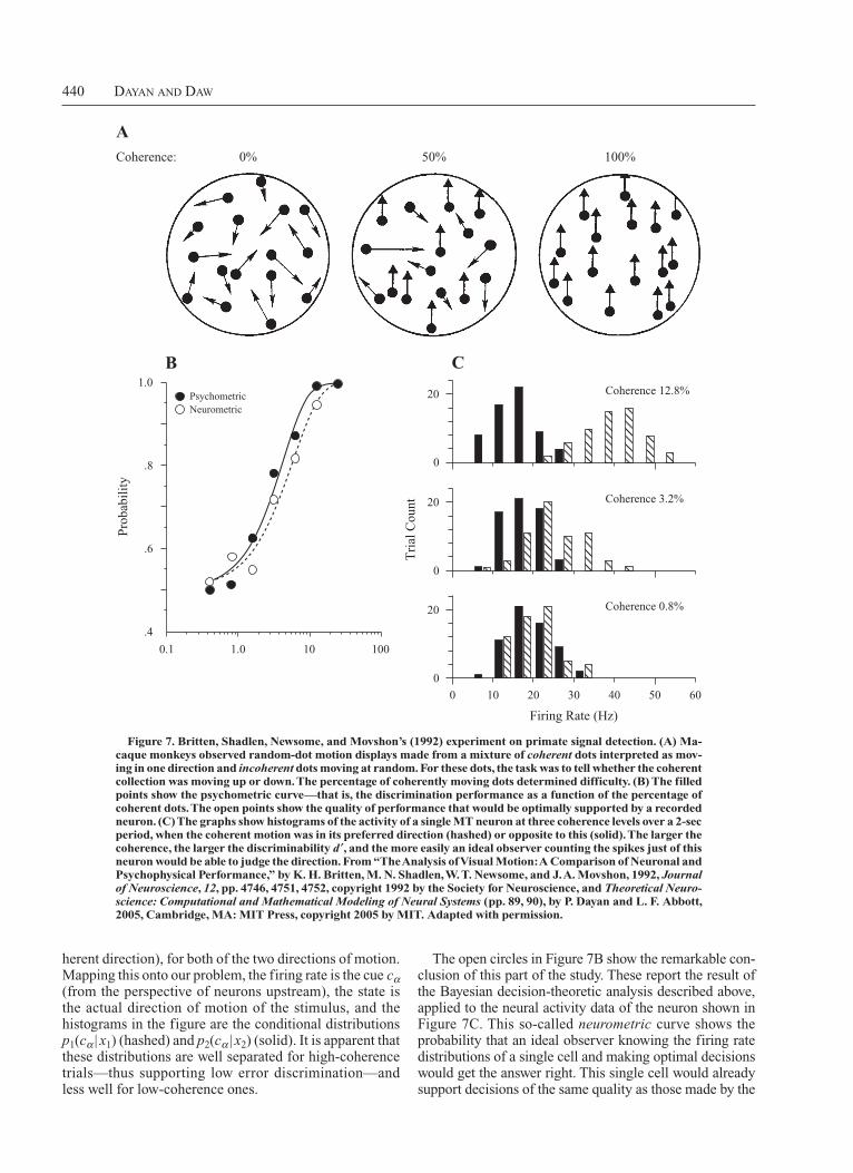
tection Theory section. Here, subjects start at xβ ∈{x3,x4} and again see a cue (referred to as cβ) that only partially distinguishes these states. They could choose L (which is correct at x3), R (correct at x4), or C, which incurs a small penalty (20.1), but delivers them to xα ∈{x1,x2}. Choos­ing C might be wise, if the cue available there cα (assumed to be suitably independent of cβ) better resolves their state uncertainty (i.e., making them more sure about which of x1 or x2 they occupy than they were between x3 and x4), and, thus, more certain to get the reward for choosing L or R according to their beliefs. The choice of C is called probing and can be considered to be a form of exploration.

The Bayesian decision­theoretic ideas articulated in the Markov Decision Problem section extend smoothly to this case, just taking into account the idea that the subject’s state should actually be its subjective belief state, given its observations. We first will consider the evolution of the belief state and then will see how this is employed to make optimal decisions. The graphs in Figure 9 refer to the Gaussian likelihood distributions used above and shown in Figure 8.

The case for x3 and x4 here is just the same as that for x1 and x2 in the Signal Detection Theory section. Given cβ, the posterior probability P(x3 | cβ) of being in x3 is given by Bayes’ rule, just as in Equation 10, proportional to the prior P(x3) and the likelihood p3(cβ| x3).

Now by choosing C at the first stage, the subject will ob­serve cα at xα ∈{x1,x2}; given this observation, it is again

whole monkey. Of course, the monkey’s problem is to pick out the cells of this caliber (and particularly, collections of cells whose activity is as independent as possible, given the motion direction; Shadlen et al., 1996), integrate their activity over the duration of the trial, and limit the ability of noise to affect their actual decisions. The difficulty of doing these things should mitigate our surprise that the overall performance of the monkey is not substantially better than that of a single, somewhat randomly recorded neuron.

TEMPORAL STATE UNCERTAINTy

The examples of the last two sections can be combined to show how belief state estimation and reinforcement learning can be combined to find optimally exploitative decisions in POMDPs. This is exemplified by the other version of the task shown in Figure 1B, in which mon­keys have to choose not only the direction of the motion, but also when they are sufficiently confident to make this choice. Here, they must balance the benefits of mak­ing their decision early—namely, avoiding the costs of waiting—against the change of making the wrong deci­sion and getting no reward at all.

The Computational ProblemFigures 8A and 8B show a version of the task that com­

bines some of the MDP as pects of the Markov Decision Problem section with the state uncertainty of the Signal De­

0 5 10 0 5 100 5 10RLRL

cc

A B

RL

x1 x2

c

r1(L) = 1 r1(R) = 0 r2(L) = 0 r2(R) = 1

p1(c|x1) p2(c|x2)

rc (L) = {0,1} rc (R) = {0,1}

0 5 10 0 5 100 5 10RLRL

cc xβ

RL

x3 x4

cβ

r3(L) = 1 r3(R) = 0 r2(L) = 0 r4(R) = 1

p3(c|x3) p4(c|x4)

p(cβ|xi)

rcβ(L) = {0,1} rcβ

(R) = {0,1}

r3(C) = –0.1 r3(C) = –0.1 rcβ(C) = –0.1

α α

α

p(c |xi)α

xα

Figure 8. Information integration and probing. Subjects start at xβ ∈{x3,x4}, but with uncertainty due to an aliased cue cβ, and can either act (perform L or R) immedi ately or perform action C, which incurs a small cost rcβ 5

20.1, but takes them to xα ∈{x1,x2}, where a new, independent ob-servation cα can help resolve the uncertainty as to which of L or R would be better. As in Figure 5, panel A shows the ob jective state and outcomes; panel B shows similar quantities from a subjective viewpoint. The distributions show how the cues are related to the states. This is a simple task, since the transitions are deterministic p31 5 p42 5 1.

442 Dayan anD Daw

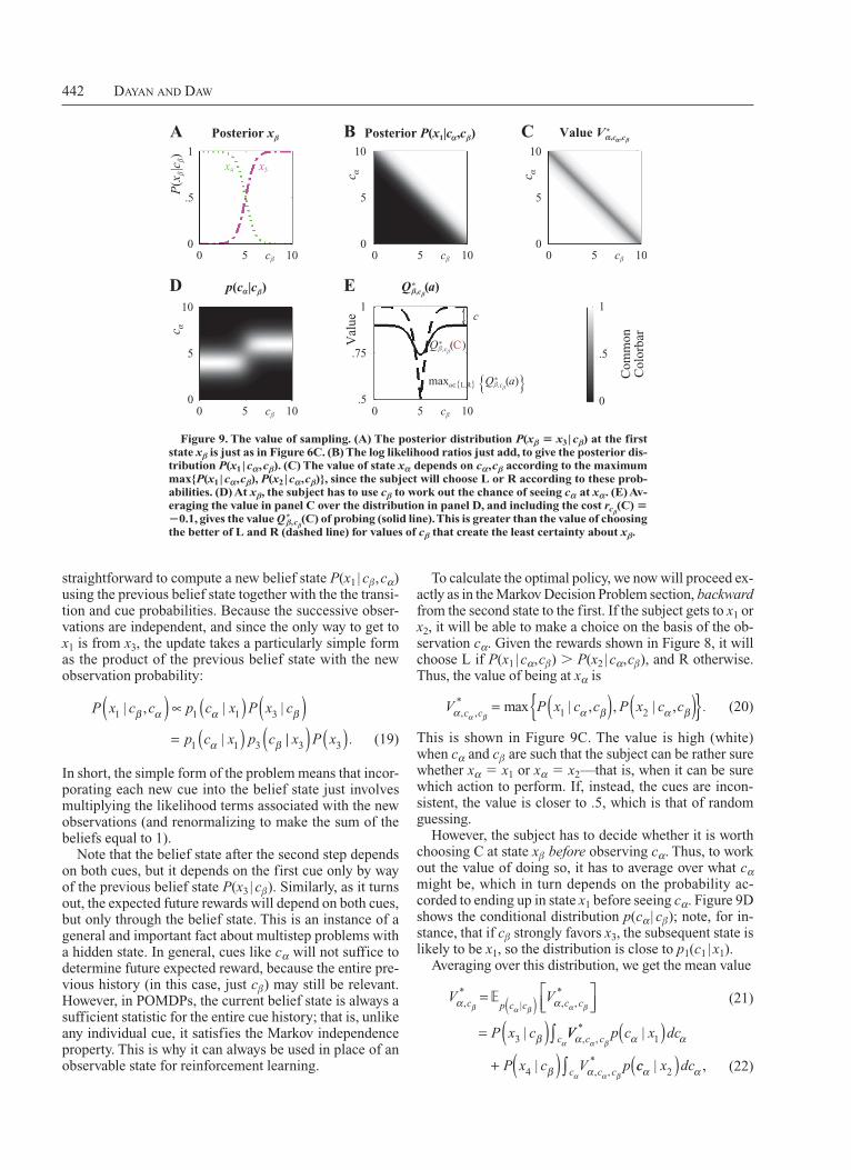
To calculate the optimal policy, we now will proceed ex­actly as in the Markov Decision Problem section, backward from the second state to the first. If the subject gets to x1 or x2, it will be able to make a choice on the basis of the ob­servation cα. Given the rewards shown in Figure 8, it will choose L if P(x1 | cα,cβ) . P(x2 | cα,cβ), and R otherwise. Thus, the value of being at xα is

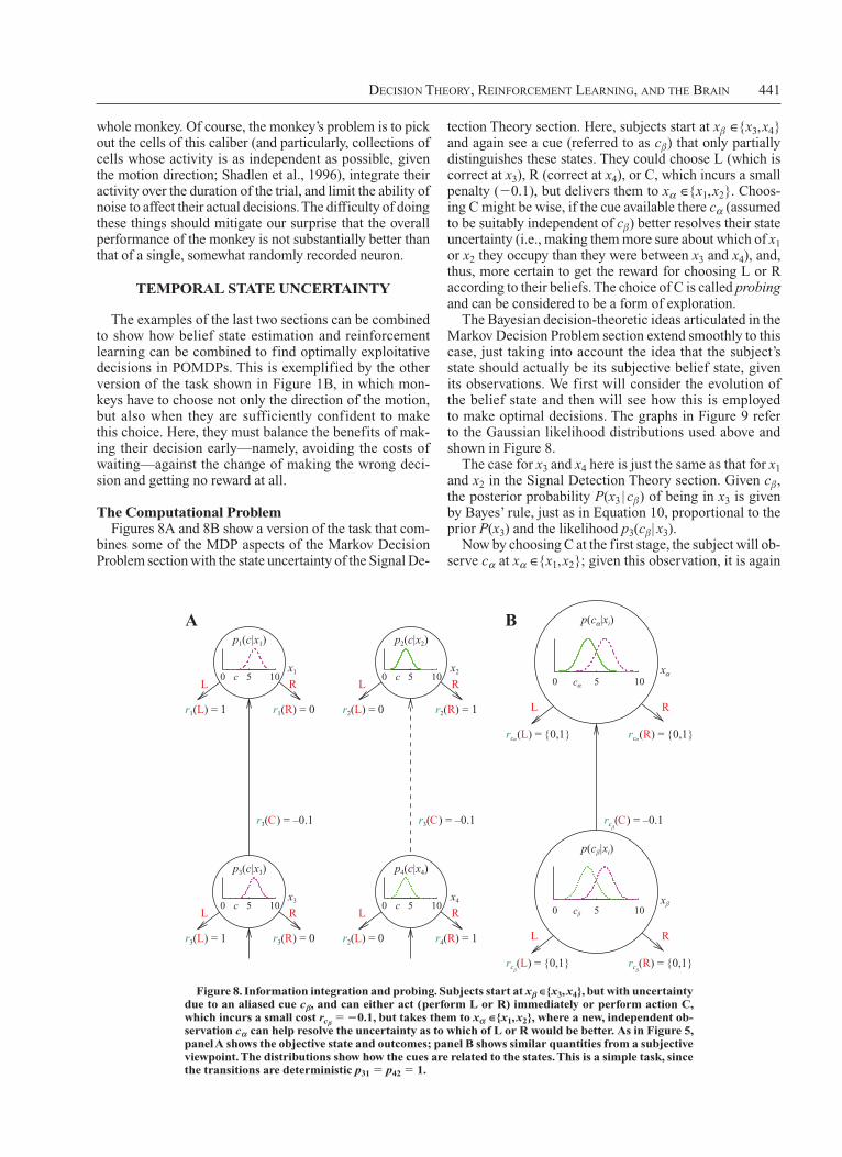
V P x c c P x c cc cα α β α βα β, , max , , ,* .= ( ) ( ){ }1 2| | (20)

This is shown in Figure 9C. The value is high (white) when cα and cβ are such that the subject can be rather sure whether xα 5 x1 or xα 5 x2—that is, when it can be sure which action to perform. If, instead, the cues are incon­sistent, the value is closer to .5, which is that of random guessing.

However, the subject has to decide whether it is worth choosing C at state xβ before observing cα. Thus, to work out the value of doing so, it has to average over what cα might be, which in turn depends on the probability ac­corded to ending up in state x1 before seeing cα. Figure 9D shows the conditional distribution p(cα | cβ); note, for in­stance, that if cβ strongly favors x3, the subsequent state is likely to be x1, so the distribution is close to p1(c1 | x1).

Averaging over this distribution, we get the mean value

(21)

V V

P x c

c p c c c c

c

α α

β

β α β α β

α

, | , ,* *=

= ( )( )

∫

3 | VV p c x dc

P x c V p

c c

c c c

α α α

β α

α β

α α β

, ,

, ,

*

*

|

|

1

4

( )+ ( ) ∫ cc x dcα α| 2( ) , (22)

straightforward to compute a new belief state P(x1 | cβ,cα) using the previous belief state together with the the transi­tion and cue probabilities. Because the successive obser­vations are independent, and since the only way to get to x1 is from x3, the update takes a particularly simple form as the product of the previous belief state with the new observation probability:

P x c c p c x P x c

p c x p c

1 1 1 3

1 1 3

| | |

|

β α α β

α β

,( ) ∝ ( ) ( )= ( ) || x P x3 3( ) ( ) . (19)

In short, the simple form of the problem means that incor­porating each new cue into the belief state just involves multiplying the likelihood terms associated with the new observations (and renormalizing to make the sum of the beliefs equal to 1).

Note that the belief state after the second step depends on both cues, but it depends on the first cue only by way of the previous belief state P(x3 | cβ). Similarly, as it turns out, the expected future rewards will depend on both cues, but only through the belief state. This is an instance of a general and important fact about multistep problems with a hidden state. In general, cues like cα will not suffice to determine future expected reward, because the entire pre­vious history (in this case, just cβ) may still be relevant. However, in POMDPs, the current belief state is always a sufficient statistic for the entire cue history; that is, unlike any individual cue, it satisfies the Markov independence property. This is why it can always be used in place of an observable state for reinforcement learning.

Com

mon

Col

orba

r

C

0

5

10

0

.5

1

0 5 100

.5

1

A

cβ

Posterior xβ

P(x

β|c β

)x3x4

D

0 5 100

5

10

cβ

0 5 10cβ 0 5 10cβ

0 5 10cβ

0

5

10

B

Val

ue

.5

.75

1

E

c

Qβ*,cβ

(a)

Qβ*

,cβ(C)

maxa∈{L,R} {Qβ*

,cβ(a)}

Value V *,c ,cβα α

Posterior P(x1|c ,cβ)α

c α

p(c |cβ)α

c α c α

Figure 9. The value of sampling. (A) The posterior distribution P(xβ 5 x3 | cβ) at the first state xβ is just as in Figure 6C. (B) The log likelihood ratios just add, to give the posterior dis-tribution P(x1 | cα,cβ). (C) The value of state xα depends on cα,cβ according to the maximum max{P(x1 | cα,cβ), P(x2 | cα,cβ)}, since the subject will choose L or R according to these prob-abilities. (D) At xβ, the subject has to use cβ to work out the chance of seeing cα at xα. (E) Av-eraging the value in panel C over the distribution in panel D, and including the cost rcβ

(C) 5 20.1, gives the value Q*β,cβ

(C) of probing (solid line). This is greater than the value of choosing the better of L and R (dashed line) for values of cβ that create the least certainty about xβ.

Decision Theory, reinforcemenT Learning, anD The Brain 443

tory grows over time (the number of steps in the prob­lem might be much larger than the two here) and so the dimensionality of the optimization problem grows also. It also poses severe demands on short­term memory. In general, it is not possible to represent optimal value func­tions and policies with only a few basis functions, as in Equation 18.

The alternative representation, which we have stressed, is to note that, given a model, the full history of ob­servations can be summarized in a single belief state, P(xτ| {c1, . . . , cτ}), which can then be updated recursively at each step. This has the advantage of not changing di­mension over time and, thus, also not placing such an obvious load on working memory. However, like the cue history (but unlike the states of an observable MDP), this probability distribution is still a multidimensional, con­tinuous object, which makes learning values and policies as functions of it still difficult in general.

Since belief states of this sort are computed by infer­ence using a model, model­free methods cannot create them and, therefore, generally have to work with the history­based representation. However, the Markov suffi­ciency of the belief state immediately suggests an appeal­ing hybrid of model­free and model­based approaches, whereby a model might be used only to infer the cur rent belief state and then model­free methods are used to learn values or policies on the basis of it (Chrisman, 1992; Daw, Courville, & Touretzky, 2006). This view separates the problem of state representation from that of policy learn­ing: The use of a model for state inference addresses the insufficiency of the immediate cues c. Having done so, it may nevertheless be advantageous to use computation­ally simple model­free methods (rather than laborious model­based dynamic programming) to obtain values or policies.

When belief states are used, algorithmic issues also arise in updating them using Equation 19. No tably, it may be simpler to represent the belief state by its logarithm, in which case the multiplica tion to integrate each new ob­servation becomes just a sum. The idea of manipulating probabilities in the log domain is ubiquitous in models of the neural basis of this sort of reasoning (Ma, Beck, Latham, & Pouget, 2006; Rao, 2004), including the one discussed next. However, it is important to note that in gen eral, belief updates involve not just multiplication, as above, but also addition, which means that the expression is no longer simplified by a logarithm. For instance, if it were possible to get to state x1 from both x3 and x4, Equa­tion 19 would sum over both possibilities:

P x c c p c x P x x P x c

p c

1 1 1 1 3 3

1

| | | |

|

β α α β

α

,( ) ∝ ( ) ( ) ( )+ xx P x x P x c1 1 4 4( ) ( ) ( )| | β . (26)

Purely additive accumulation is therefore limited to a class of problems with constrained tran sition matrices and inde­pendent observations. Also, it is only in a two­alternative case that the normalization may, in general, be eliminated by tracking the ratio, or log ratio, of the probability of the states, as in Equation 11.

since the transitions can occur only from x3 x1 or x4 x2. This is the exact equivalent of Equations 3A and 3B, except that taking an expectation over the belief state requires an integral (because it is continuous) rather than a discrete sum.

The last step is to work out the values of executing each action at xβ. For action C, from Equation 4 and the transi­tion probabilities:

Q r V Vc c c cβ α αβ β β β, , ,C C* * *. .( ) = ( ) + = − +0 1 (23)

This value is shown as the solid line in Figure 9E. It is high when the subject can expect to be relatively certain about the identity of xα and low when this is not likely. The maximum value is 1 1 rcβ(C) 5 0.9, given the cost 20.1 of probing.

The expected values to the subject of performing L or R at xβ are

Q P x c Q P x cc cβ β β ββ β, ,L R ,* *( ) = ( ) ( ) = ( )3 4| | (24)

which are the exact analogues of the Q*cα(a) terms in Equa­tion 12. The dashed line in Figure 9E shows the value of the better of L and R. This is near 0.5 for intermediate val­ues of cβ, where the subject will be very unsure between x3 and x4 and, thus, between the actions. In this region, action C is preferable because the additional observation cα is likely to provide additional certainty and a better choice at the next step, even weighed against the 20.1 cost of C.

Combining the equations above, the subject should choose C if

max ,

max

P x c P x c

P xp c c

3 4

10 1

| |

|

β β

α β

( ) ( ){ } <

− + ( ). || |c c P x c cα β α β, , , ;( ) ( ){ }

2

(25)

that is, if the benefit of the added certainty about being in x1 or x2 outweighs the cost 20.1 of sampling.

The two points at which the two curves in Figure 9E cross are thresholds cl and ch in cβ, such that probing is preferred when cl , cβ , ch. We will see that this sort of test is quite general for problems with this character, although the thresholds are normally applied to the belief states associated with the observations, rather than to the observations themselves.

Algorithmic IssuesThe case of temporally extended choices in the face of

incomplete knowledge is known to pose severe computa­tional complications as the number of states grows larger than that for the simple problem described here. The dif­ficulties have to do with the definition of the state of the subject. There are actually two ways to look at this, both of which are problematic. One way is to see the state as a summary of the entire history (and, for planning, the future) of the observations (say, cβ, cα, . . .) of the agent. Indeed, we indexed value functions such as V *α,cα,cβ

by this history. The trouble with this representation is that the his­

444 Dayan anD Daw

ratios of all the pieces of evidence cT 5 {c1, . . . , cT} given the two state possibilities, which can be written

T TT

T

p c c x

p c c xc( ) =

( )( )

=

log, ,

, ,

lo

L

R

1

1

...

...

|

|

gg

,

L

R

p c x

p c x

c

τ

ττ

τ ττ

|

|

( )( )

= ( )∑

∑

Finally, in discussing partially observable situations, we have so far assumed that the model is known. In general, of course, this might also be learned from experience. In the observable MDP, this simply requires counting state transitions (Equation 6B); however, when states are not directly observable, their transitions obviously cannot be counted. One family of algorithms for learning a model in the face of hidden states involves so­called expecta­tion maximization methods (Demp ster, Laird, & Rubin, 1977). The algorithm takes a starting guess at a model and improves it, using two steps. In the first, the expectation phase, the model is assumed to be correct, and the infer­ence algorithms we have already discussed are used to infer which (hidden) state trajectory was re sponsible for observed cues. In the second, maximization phase, these beliefs about the hidden trajectory are treated as being cor­rect, and then the best model to account for them is inferred using a counting process analogous to Equations 6A and 6B. These phases are repeatedly alternated, and it can be shown that each iteration improves the model, in the sense of making the observed data more likely under it (Neal & Hinton, 1998). In actuality, these model­learning methods require substantial data, are difficult to extend to practical online learning from an ongoing sequence of experience, and are prone to getting stuck at suboptimal models that occupy local maxima of the hill­climbing update.

Psychology and Neuroscience: Drift Diffusion Decision Making

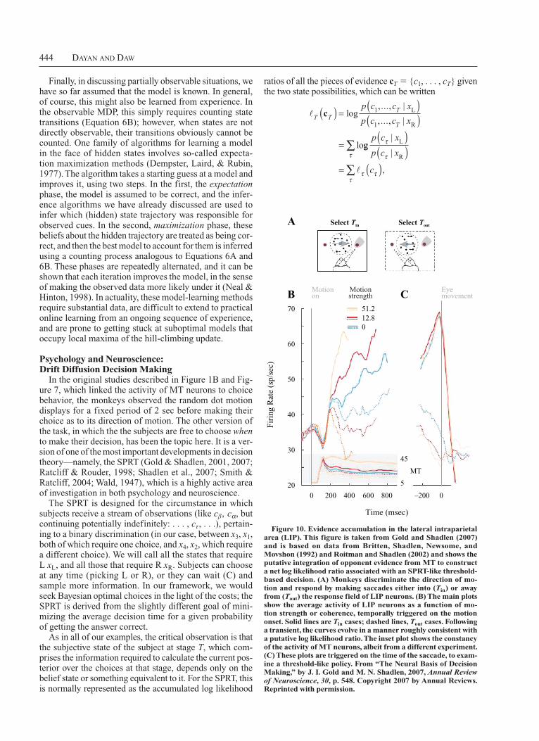
In the original studies described in Figure 1B and Fig­ure 7, which linked the activity of MT neurons to choice behavior, the monkeys observed the random dot motion displays for a fixed period of 2 sec before making their choice as to its direction of motion. The other version of the task, in which the the subjects are free to choose when to make their decision, has been the topic here. It is a ver­sion of one of the most important developments in decision theory—namely, the SPRT (Gold & Shadlen, 2001, 2007; Ratcliff & Rouder, 1998; Shadlen et al., 2007; Smith & Ratcliff, 2004; Wald, 1947), which is a highly active area of investigation in both psychology and neuroscience.

The SPRT is designed for the circumstance in which subjects receive a stream of observations (like cβ, cα, but continuing potentially indefinitely: . . . , cτ, . . .), pertain­ing to a binary discrimination (in our case, between x3, x1, both of which require one choice, and x4, x2, which require a different choice). We will call all the states that require L xL, and all those that require R xR. Subjects can choose at any time (picking L or R), or they can wait (C) and sample more information. In our framework, we would seek Bayesian optimal choices in the light of the costs; the SPRT is derived from the slightly different goal of mini­mizing the average decision time for a given probability of getting the answer correct.

As in all of our examples, the critical observation is that the subjective state of the subject at stage T, which com­prises the information required to calculate the current pos­terior over the choices at that stage, depends only on the belief state or something equivalent to it. For the SPRT, this is normally represented as the accumulated log likelihood

A

B C

Select Tin Select Tout

Motionon

Motionstrength

Eyemovement

51.212.80

70

60

50

40

30

20

Fir

ing

Rat

e (s

p/se

c)

45

5

MT

0 200 400 600

Time (msec)

800 –200 0

Figure 10. Evidence accumulation in the lateral intraparietal area (LIP). This figure is taken from Gold and Shadlen (2007) and is based on data from Britten, Shadlen, Newsome, and Movshon (1992) and Roitman and Shadlen (2002) and shows the putative integration of opponent evidence from MT to construct a net log likelihood ratio associated with an SPRT-like threshold-based decision. (A) Monkeys discriminate the direction of mo-tion and respond by making saccades either into (Tin) or away from (Tout) the response field of LIP neurons. (B) The main plots show the average activity of LIP neurons as a function of mo-tion strength or coherence, temporally triggered on the motion onset. Solid lines are Tin cases; dashed lines, Tout cases. Following a transient, the curves evolve in a manner roughly consistent with a putative log likelihood ratio. The inset plot shows the constancy of the activity of MT neurons, albeit from a different experiment. (C) These plots are triggered on the time of the saccade, to exam-ine a threshold-like policy. From “The Neural Basis of Decision Making,” by J. I. Gold and M. N. Shadlen, 2007, Annual Review of Neuroscience, 30, p. 548. Copyright 2007 by Annual Reviews. Reprinted with permission.

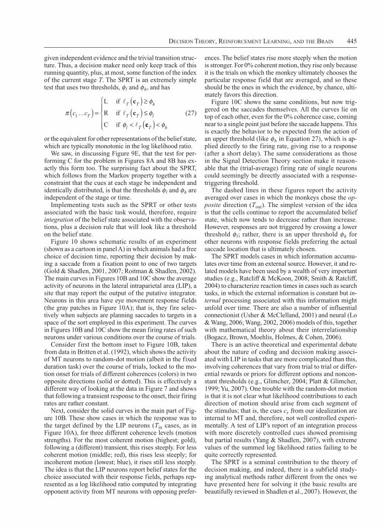
Decision Theory, reinforcemenT Learning, anD The Brain 445

ences. The belief states rise more steeply when the motion is stronger. For 0% coherent motion, they rise only be cause it is the trials on which the monkey ultimately chooses the particular response field that are averaged, and so these should be the ones in which the evidence, by chance, ulti­mately favors this direction.

Figure 10C shows the same conditions, but now trig­gered on the saccades themselves. All the curves lie on top of each other, even for the 0% coherence case, coming near to a single point just before the saccade happens. This is exactly the behavior to be expected from the action of an upper threshold (like φh in Equation 27), which is ap­plied directly to the firing rate, giving rise to a response (after a short delay). The same considerations as those in the Signal Detection Theory section make it reason­able that the (trial­average) firing rate of single neurons could seemingly be directly associated with a response­ triggering threshold.

The dashed lines in these figures report the activity averaged over cases in which the monkeys chose the op-posite direction (Tout). The simplest version of the idea is that the cells continue to report the accumulated belief state, which now tends to decrease rather than increase. However, responses are not triggered by crossing a lower threshold φ l; rather, there is an upper threshold φh for other neurons with response fields preferring the actual saccade location that is ultimately chosen.

The SPRT models cases in which information accumu­lates over time from an external source. However, it and re­lated models have been used by a wealth of very important studies (e.g., Ratcliff & McKoon, 2008; Smith & Ratcliff, 2004) to characterize reaction times in cases such as search tasks, in which the external information is constant but in-ternal processing associated with this information might unfold over time. There are also a number of influential connectionist (Usher & McClelland, 2001) and neural (Lo & Wang, 2006; Wang, 2002, 2006) models of this, together with mathematical theory about their interrelationship (Bogacz, Brown, Moehlis, Holmes, & Cohen, 2006).

There is an active theoretical and experimental debate about the nature of coding and decision making associ­ated with LIP in tasks that are more complicated than this, involving coherences that vary from trial to trial or differ­ential rewards or priors for different options and noncon­stant thresholds (e.g., Glimcher, 2004; Platt & Glimcher, 1999; Yu, 2007). One trouble with the random­dot motion is that it is not clear what likelihood contributions to each direction of motion should arise from each segment of the stimulus; that is, the cues cτ from our idealization are internal to MT and, therefore, not well controlled experi­mentally. A test of LIP’s report of an integration process with more discretely controlled cues showed promising but partial results (Yang & Shadlen, 2007), with extreme values of the summed log likelihood ratios failing to be quite cor rectly represented.

The SPRT is a seminal contribution to the theory of decision making, and indeed, there is a sub field study­ing analytical methods rather different from the ones we have presented here for solv ing it (the basic results are beautifully reviewed in Shadlen et al., 2007). However, the

given independent evidence and the trivial transition struc­ture. Thus, a decision maker need only keep track of this running quantity, plus, at most, some function of the index of the current stage T. The SPRT is an extremely simple test that uses two thresholds, φ l and φh, and has

π

φ

φ

φ

c cT

T T h

T T l

l T

1 ...( ) =

( ) ≥

( ) ≤

<

L if

R if

C if

c

c

ccT h( ) <

φ

(27)

or the equivalent for other representations of the belief state, which are typically monotonic in the log likelihood ratio.

We saw, in discussing Figure 9E, that the test for per­forming C for the problem in Figures 8A and 8B has ex­actly this form too. The surprising fact about the SPRT, which follows from the Markov property together with a constraint that the cues at each stage be independent and identically distributed, is that the thresholds φ l and φh are independent of the stage or time.

Implementing tests such as the SPRT or other tests associated with the basic task would, therefore, require integration of the belief state associated with the observa­tions, plus a decision rule that will look like a threshold on the belief state.

Figure 10 shows schematic results of an experiment (shown as a cartoon in panel A) in which animals had a free choice of decision time, reporting their decision by mak­ing a saccade from a fixation point to one of two targets (Gold & Shadlen, 2001, 2007; Roitman & Shadlen, 2002). The main curves in Figures 10B and 10C show the average activity of neurons in the lateral intraparietal area (LIP), a site that may report the output of the putative integrator. Neurons in this area have eye movement response fields (the gray patches in Figure 10A); that is, they fire selec­tively when subjects are planning saccades to targets in a space of the sort employed in this experiment. The curves in Figures 10B and 10C show the mean firing rates of such neurons under various conditions over the course of trials.

Consider first the bottom inset to Figure 10B, taken from data in Britten et al. (1992), which shows the activity of MT neurons to random­dot motion (albeit in the fixed duration task) over the course of trials, locked to the mo­tion onset for trials of different coherences (colors) in two opposite directions (solid or dotted). This is effectively a different way of looking at the data in Figure 7 and shows that following a transient response to the onset, their firing rates are rather constant.

Next, consider the solid curves in the main part of Fig­ure 10B. These show cases in which the re sponse was to the target defined by the LIP neurons (Tin cases, as in Figure 10A), for three different coherence levels (motion strengths). For the most coherent motion (highest; gold), following a (different) transient, this rises steeply. For less coherent motion (middle; red), this rises less steeply; for incoherent motion (lowest; blue), it rises still less steeply. The idea is that the LIP neurons report belief states for the choice associated with their response fields, perhaps rep­resented as a log likelihood ratio com puted by integrating opponent activity from MT neurons with opposing prefer­

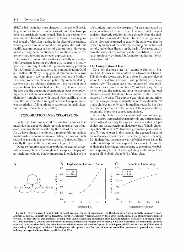
446 Dayan anD Daw

rules, might improve the prospects for earning reward on subsequent trials. This is a difficult balance, but its elegant decision­ theoretic solution follows directly from the anal­ysis we have already developed. In par ticular, ignorance of the rules can be treated in exactly the same way that we treated ignorance of the state: by planning on the basis of beliefs, rather than directly on the basis of observations. In turn, the value of exploration can be quantified just as we have previously evaluated information­gathering ( prob-ing) actions like C.

The Computational IssueConsider the one­state (x1) example shown in Fig­

ure 11A, known in this context as a two­armed bandit. This time, the rewards are binary (0 or 1), and a choice of action L or R delivers reward 1 with probability pL or pR, respectively. The agent starts out ignorant of these prob­abilities, has a limited number (N ) of trials (say, 50) in which to play the game, and aims to maximize the total obtained reward. The dotted lines emphasize the iterative nature of the task. The explore/exploit dilemma arises here because pL and pR remain the same throughout the 50 trials; choices not only earn immediate rewards, but also help the subject to learn the values of these probabilities, potentially improving subsequent choices.

If the subject starts with the additional prior knowledge that pL and pR were each drawn uni formly and independently between 0 and 1, clearly the expected value of either is .5 per choice, and the expected cumulative reward of blindly choos­ing either 50 times is 25. However, given two options whose payoffs were chosen in this manner, the expected value of the better one (whichever it is) is actually higher—namely, 2/3. If, therefore, the subject was told which one is better, he or she could exploit it and expect to earn about 33 rewards. Without this knowledge, but choosing so as optimally to bal­ance exploring to find it and exploiting it, the subject can expect still to obtain about 96% of that value.

SPRT is brittle, in that most changes to the task will break its guarantees. In fact, even the case of more than two op­tions is surprisingly complicated. This is one reason why here, we have framed this problem in terms of a more gen­eral model of decision making in the face of uncertainty, which gives a similar account of this particular task but readily accommodates a host of elaborations. However, as has already been mentioned, the solutions can be ex­tremely hard to compute or even approx imate.

Viewing the random­dots task as a partially observable reinforcement learning problem also suggests broadly how the brain might solve the policy­learning problem for it (Ahmadi & Latham, personal communication; Gold & Shadlen, 2002): by using general reinforcement learn­ing techniques—such as those described in the Markov Decision Problem section and putatively implemented by systems such as midbrain dopamine—over a belief state representation (as described here for LIP). In other work, the idea that the dopamine system might learn by employ­ing a belief state representation has also been used to ex­plain how it might cope with partial observability arising from the unpredictable timing of cues and to explain some characteristics of dopaminergic responses in such situa­tions (Daw, Courville, et al., 2006).

ExPLORATION AND ExPLOITATION

So far, we have considered exploitation: choices that maximize the expected single­episode return, given what­ever is known about the rules by the time of that episode. As we have already men tioned, a more ambitious subject might wish to maximize lifetime utility, earning as much reward as possible over a whole series of episodes. This is exactly the goal in the task shown in Figure 1C.

Doing so requires balancing exploitation against explo-ration: taking choices that might not be expected to pay off as much immediately but, by improving knowledge of the

CBA

0 .2 .4 .6 .8 10.4

0.5

0.6

0.7

0.8

0.9

Expected pL

Val

ue p

er C

hoic

e

LeftRight

0 .02 .04 .06 .080.4

0.45

0.5

0.55

0.6

0.65

Uncertainty About pL

Val

ue p

er C

hoic

e

Benefits of UncertaintyExploration–Corrected Value

x1

L R

LeftRight

P(r1(L) = 1) = pL pR = P(r1(R) = 1)

Figure 11. (A) Two-armed bandit task. For each episode, the agent can choose L or R, which pay off with (initially unknown) prob-abilities pL and pR. Subjects have a fixed total number of choices N (emphasized by the dotted lines) and seek to optimize their summed reward. (B) The value of exploration: The long-term value of choosing uncertain option L as a function of its expected immediate pay-off. (The cumulative Q value over 50 choices is plotted normalized to a per choice value.) Note that even when the immediate payoff is expected to be less than 50%, the value lies above that for repeated choice of option R, which pays off 50% for certain. (C) The value of uncertainty: The long-term value of choosing uncertain option L as a function of how uncertain it is (measured as posterior variance), holding the expected immediate payoff fixed at 50%.

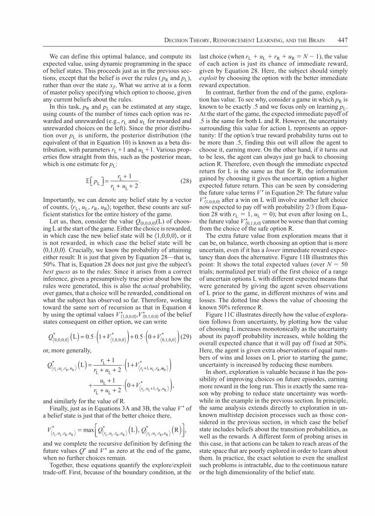
Decision Theory, reinforcemenT Learning, anD The Brain 447

last choice (when rL 1 uL 1 rR 1 uR 5 N 2 1), the value of each action is just its chance of immediate reward, given by Equation 28. Here, the subject should simply exploit by choosing the option with the better immediate reward expectation.

In contrast, further from the end of the game, explora­tion has value. To see why, consider a game in which pR is known to be exactly .5 and we focus only on learning pL. At the start of the game, the expected immediate payoff of .5 is the same for both L and R. However, the uncertainty sur rounding this value for action L represents an oppor­tunity: If the option’s true reward probability turns out to be more than .5, finding this out will allow the agent to choose it, earning more. On the other hand, if it turns out to be less, the agent can always just go back to choosing action R. Therefore, even though the immediate expected return for L is the same as that for R, the information gained by choosing it gives the uncertain option a higher expected future return. This can be seen by considering the future value terms V * in Equation 29: The future value V *⟨1,0,0,0⟩ after a win on L will involve another left choice now expected to pay off with probability 2/3 (from Equa­tion 28 with rL 5 1, uL 5 0); but even after losing on L, the future value V *⟨0,1,0,0⟩ cannot be worse than that coming from the choice of the safe option R.

The extra future value from exploration means that it can be, on balance, worth choosing an option that is more uncertain, even if it has a lower immediate reward expec­tancy than does the alternative. Figure 11B illustrates this point: It shows the total expected values (over N 5 50 trials; normalized per trial) of the first choice of a range of uncertain options L with different expected means that were generated by giving the agent seven observations of L prior to the game, in different mixtures of wins and losses. The dotted line shows the value of choosing the known 50% reference R.

Figure 11C illustrates directly how the value of explora­tion follows from uncertainty, by plotting how the value of choosing L increases monotonically as the uncertainty about its payoff probability increases, while holding the overall expected chance that it will pay off fixed at 50%. Here, the agent is given extra observations of equal num­bers of wins and losses on L prior to starting the game; uncertainty is increased by reducing these numbers.

In short, exploration is valuable because it has the pos­sibility of improving choices on future episodes, earning more reward in the long run. This is exactly the same rea­son why probing to reduce state uncertainty was worth­while in the example in the previous section. In principle, the same analysis extends directly to exploration in un­known multistep decision processes such as those con­sidered in the previous section, in which case the belief state includes beliefs about the transition probabilities, as well as the rewards. A different form of probing arises in this case, in that actions can be taken to reach areas of the state space that are poorly explored in order to learn about them. In practice, the exact solution to even the smallest such problems is intractable, due to the continuous nature or the high dimensionality of the belief state.

We can define this optimal balance, and compute its expected value, using dynamic programming in the space of belief states. This proceeds just as in the previous sec­tions, except that the belief is over the rules ( pR and pL), rather than over the state xβ. What we arrive at is a form of master policy specifying which option to choose, given any current beliefs about the rules.

In this task, pR and pL can be estimated at any stage, using counts of the number of times each option was re­warded and unrewarded (e.g., rL and uL for rewarded and unrewarded choices on the left). Since the prior distribu­tion over pL is uniform, the posterior distribution (the equivalent of that in Equation 10) is known as a beta dis­tribution, with parameters rL11 and uL11. Various prop­erties flow straight from this, such as the posterior mean, which is one estimate for pL:

pr

r uLL

L L

=+

+ +1

2. (28)

Importantly, we can denote any belief state by a vector of counts, ⟨rL, uL, rR, uR⟩; together, these counts are suf­ficient statistics for the entire history of the game.

Let us, then, consider the value Q⟨0,0,0,0⟩(L) of choos­ing L at the start of the game. Either the choice is rewarded, in which case the new belief state will be ⟨1,0,0,0⟩, or it is not rewarded, in which case the belief state will be ⟨0,1,0,0⟩. Crucially, we know the probability of attaining either result: It is just that given by Equation 28—that is, 50%. That is, Equation 28 does not just give the subject’s best guess as to the rules: Since it arises from a correct inference, given a presumptively true prior about how the rules were generated, this is also the actual probability, over games, that a choice will be rewarded, conditional on what the subject has observed so far. Therefore, working toward the same sort of recursion as that in Equation 4 by using the optimal values V *⟨1,0,0,0⟩,V *⟨0,1,0,0⟩ of the belief states consequent on either option, we can write

Q V V0 0 0 0 1 0 0 0 1 0

0 5 1 0 5 0, , , ,0, , , ,

L* *. .( ) = ⋅ +( ) + ⋅ +,,0

*( ) (29)

or, more generally,

Qr

r uV

r u r u r u rL L R R L L R, , ,L

L L, , ,

L* ( ) =+

+ +⋅ + +

1

21

1 uu

r u r u

u

r uV

R

L L R R

L

L L, , ,

,

*

*

( )+

++ +

⋅ +( )+1

20

1

and similarly for the value of R.Finally, just as in Equations 3A and 3B, the value V * of

a belief state is just that of the better choice there,

V Q Qr u r u r u r u r u rL L R R L L R R L L R, , , , , , , ,

max L ,* *= ( ) ,, RR ,

u* ( )

and we complete the recursive definition by defining the future values Q* and V * as zero at the end of the game, when no further choices remain.

Together, these equations quantify the explore/exploit trade­off. First, because of the boundary condition, at the

448 Dayan anD Daw

tors as the degree of randomness or the lucrativity of the uncertainty bonuses in order to perform well. Although finding the optimal exploratory policy is not normally considered a learning problem (since the goal, after all, is lifetime optimality), learning of a sort is implicated in tuning the parameters of the approximate approaches to improve their performance.

Psychology and NeuroscienceOutside the field of ethology (e.g., Mangel & Clark,

1989; McNamara & Houston, 1980; Pyke, 1984) exempli­fied by some early work on the exploration of birds (Krebs, Kacelnik, & Taylor, 1978), there is relatively little direct evidence as to how animals or humans explore. There are, however, a number of models. In this vein, Kakade and Dayan (2002) noted that dopamine neurons respond to novel but affectively neutral stimuli with a burst–pause re­sponse; they suggested that this pattern could be explained if the neurons were reporting the effect on reward predic­tion error of stimuli that were up­valued due to a novelty or uncertainty bonus.

Subsequently, in the task shown in Figure 1C, Daw, O’Doherty, et al. (2006) sought to test a similar idea more directly, in an fMRI study of humans making choices for money in a four­armed bandit task similar to the two­armed bandit task analyzed above. Subjects had additional uncertainty and pressure to explore, because the bandits’ values were constantly changing. The authors sought to quantify the effect of this uncertainty on exploratory choices by fitting subjects’ trial­by­trial behavior with a reinforcement learning model incorporating uncertainty bonuses but found no such influence. Instead, the subjects’ exploration was best explained by a random exploration model, the so­called softmax, which, for two choices, in­volves a variant on Equation 8 with

P a Q L Q Rr u r u r u r u1 =( ) = ( ) − ( )

L

L L R R L L R R, , , , , ,σ β

{ },

where β . 0 regulates the strength of competition—that is, the extent to which a small difference in expected val­ues of the actions translates into a large difference in their probability of choice. This parameter is therefore another of the more primitive ways of trading off exploration and exploita tion.

The neural data supported a similar conclusion. Bonus models such as that of Kakade and Dayan (2002) (or in­deed, the optimal decision theoretic analysis) quantify the value of exploration and exploitation in terms of a single currency of expected future reward. They therefore predict that exploratory value should be reported just as is exploi­tation—for instance, through dopamin ergic spiking. Con­trary to this expectation, Daw, O’Doherty, et al. (2006) found that although dopaminergic efferent areas such as the striatum were activated by predictions and prediction errors for money, they exhibited no additional activation that might reflect bonus values involved in exploration. Instead, separate areas—the frontal pole and, also, an area of the intraparietal cortex—were acti vated preferentially when subjects explored rather than exploited (Figure 12). Here, exploration was operationally defined as a choice

Algorithmic IssuesSo far, we have characterized the computational issues

underlying exploration as concerning ambition—that is, optimizing reward accumulated across episodes, rather than myopically exploiting within each. In this respect, the problem can be seen to relate to issues of temporal discounting: An unambitious subject is like an impatient one, who discounts future reward sharply. In practice, however, even for minimally patient subjects, the limiting constraint on exploratory behavior is more likely to be the extreme complexity of decision­theoretically optimal ex­ploration. Rather than differences in discount preferences or goals, different exploratory behaviors can arise from different algorithmic approaches to the decision problem. For instance, ignoring uncertainty about the rules is what enables many of the standard reinforcement learning algo­rithms discussed in the Markov Decision Problem section to work; but this can just as easily be viewed as a simplify­ing assumption that precludes optimal exploration, rather than as a myopic goal.

In fact, even though the decision­theoretic analysis of exploration is formally equivalent to that of partial observ­ability—–indeed, leading to similar practical problems in actually solving for the optimal policy—researchers have developed a number of special purpose approaches to the exploration problem.

First, Gittins (1989) showed how a subset of explora­tion problems could be simplified by comput ing an index, similar to a Q value, for each action separately in a smaller (although still nontrivial) subproblem. The approach takes advantage of a sort of independence between the actions aris ing from the problem structure. It works for multiarmed bandit problems of the sort described above, although only when the number of trials, N, is either in­finite (and future reward is discounted exponentially) or unknown with a constant hazard function—that is, a con­stant probability per trial of terminating.

However, most problems, including exploration in multi step decision problems, cannot be simpli fied this way. In reinforcement learning, heuristic approaches are, therefore, common, more or less qualitatively inspired by the optimal analysis above. Some approaches evalu­ate actions according to their expected exploitative value plus an uncertainty bonus intended to capture the addi­tional value of exploration (Dayan & Sejnowski, 1996; Dearden, Friedman, & Russell, 1998; Kaelbling, 1993; Sutton, 1990). Authors differ as to how uncertainty should be estimated (which is itself not simple in this context) and the exact form of bonus itself. One particularly sim­ple variation is the novelty bonus (e.g., Ng, Harada, & Russell, 1999), which approximates an uncertainty bonus for unexplored options sim ply by initializing estimates of their values “optimistically” high, encouraging their exploration until their true value is discovered.

A more primitive alternative, which is less well grounded in the analysis above, is to encourage exploration more blindly by introducing some sort of randomness into the choice process.

One aspect of all of these approximate approaches is that they typically require careful adjustment of such fac­

Decision Theory, reinforcemenT Learning, anD The Brain 449

aminergic neurons are activated by novelty (although, of course, BOLD activations are far from direct measure­ments of dopaminergic activity). One possibility, sug­gested by the Kakade and Dayan (2002) model and also by a follow­up imaging study (Wittmann, Daw, Seymour, & Dolan, 2008), is that the brain approximates the value of exploration by assigning bonuses for novelty, rather than for uncertainty. Novelty bonuses are particularly easy to compute—they require only optimistic initialization—but they are only an imperfect proxy for uncertainty. For in­stance, such bonuses would likely not be engaged by the task shown in Figure 1C and Figure 12, because the explo­ration there was mandated by changing reward probabili­ties in familiar bandits, rather than by explicit novelty.

Finally, if organisms indeed use some sort of random exploration, rather than exploration guided toward uncer­

of an option other than the one for which the subject was estimated to expect the most reward. Together with the behavioral results and other imaging find ings suggesting the involvement of anterior prefrontal areas in process­ing uncertainty (e.g., Yoshida & Ishii, 2006) and of the intraparietal cortex in belief states (as discussed above), this neural dissoci ation suggests that rather than being en­couraged by a bonus reported in a common currency with exploitative value, exploration in this task somehow draws on distinct neural processes.

It is certainly possible that high­level regulation of the sort associated with the frontal pole over rides a prepotent drive to exploit; however, we should stress that it is not clear from these data what function, if any, these areas causally contribute to exploration. It is also unclear how to rec oncile these findings with the observation that dop­

0.2

0.15

0.1

0.05

% S

igna

l Cha

nge

0

–0.05

–0.1

–0.15

–5 0 5

Time Since Choice

10 15 20

0.15

0.1

0.05

0

–0.05

–0.1

–5 0 5

Time Since Choice

10 15 20

Explore

Exploit

Figure 12. Areas differentially active during exploration. Top: Both the bilateral frontopolar cortex (rFP, lFP) and the anterior intraparietal sulcus (rIPS, lIPS) exhibited higher BOLD activity during choices estimated to be exploratory, as compared with exploitative ones. Bottom: BOLD time courses from these regions averaged over exploratory (solid) and exploitative (dashed) trials; both areas exhibit positive BOLD excursions during exploration and the opposite for exploitation. Adapted from “Corti-cal Substrates for Exploratory Decisions in humans,” by N. D. Daw, J. P. O’Doherty, P. Dayan, B. Seymour, and R. J. Dolan, 2006, Nature, 441, p. 878. Copyright 2006 by the Nature Publishing Group. Reprinted with permission.

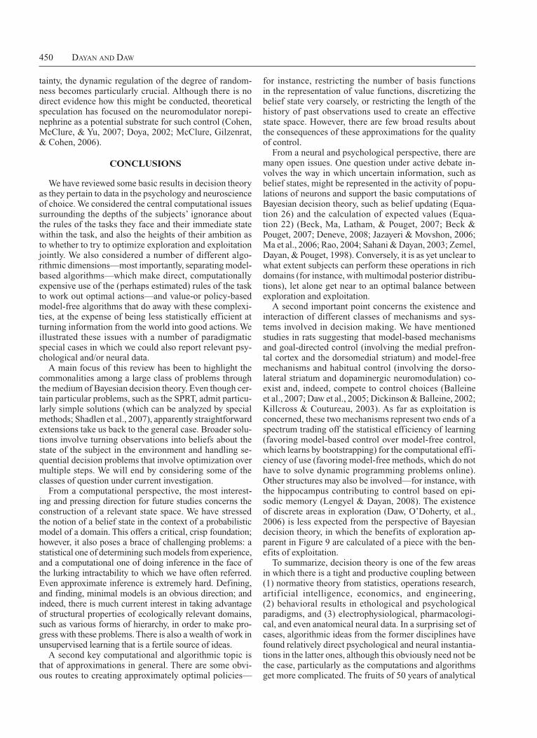
450 Dayan anD Daw

for instance, restricting the number of basis functions in the representation of value functions, discretizing the belief state very coarsely, or restricting the length of the history of past observations used to create an effective state space. However, there are few broad results about the consequences of these approximations for the quality of control.

From a neural and psychological perspective, there are many open issues. One question under active debate in­volves the way in which uncertain information, such as belief states, might be represented in the activity of popu­lations of neurons and support the basic computations of Bayesian decision theory, such as belief updating (Equa­tion 26) and the calculation of expected values (Equa­tion 22) (Beck, Ma, Latham, & Pouget, 2007; Beck & Pouget, 2007; Deneve, 2008; Jazayeri & Movshon, 2006; Ma et al., 2006; Rao, 2004; Sahani & Dayan, 2003; Zemel, Dayan, & Pouget, 1998). Conversely, it is as yet unclear to what extent subjects can perform these operations in rich domains (for instance, with multi modal posterior distribu­tions), let alone get near to an optimal balance between exploration and exploitation.

A second important point concerns the existence and interaction of different classes of mecha nisms and sys­tems involved in decision making. We have mentioned studies in rats suggest ing that model­based mechanisms and goal­directed control (involving the medial prefron­tal cortex and the dorsomedial striatum) and model­free mechanisms and habitual control (involv ing the dorso­lateral striatum and dopaminergic neuromodulation) co­exist and, indeed, compete to control choices (Balleine et al., 2007; Daw et al., 2005; Dickinson & Balleine, 2002; Killcross & Coutureau, 2003). As far as exploitation is concerned, these two mechanisms represent two ends of a spectrum trading off the statistical efficiency of learning (favoring model­based control over model­free control, which learns by bootstrapping) for the computational effi­ciency of use (favoring model­free methods, which do not have to solve dynamic programming problems on line). Other structures may also be involved—for instance, with the hippocampus contributing to control based on epi­sodic memory (Lengyel & Dayan, 2008). The existence of discrete areas in exploration (Daw, O’Doherty, et al., 2006) is less expected from the perspective of Bayesian decision theory, in which the benefits of exploration ap­parent in Figure 9 are calculated of a piece with the ben­efits of exploitation.

To summarize, decision theory is one of the few areas in which there is a tight and productive coupling between (1) normative theory from statistics, operations research, artif icial intelligence, eco nomics, and engineering, (2) behavioral results in ethological and psychological paradigms, and (3) electrophysiological, pharmacologi­cal, and even anatomical neural data. In a surprising set of cases, algorithmic ideas from the former disciplines have found relatively direct psychological and neural instantia­tions in the latter ones, although this obviously need not be the case, particularly as the computations and algorithms get more complicated. The fruits of 50 years of analytical

tainty, the dynamic regulation of the degree of random­ness becomes particu larly crucial. Although there is no direct evidence how this might be conducted, theoretical specu lation has focused on the neuromodulator norepi­nephrine as a potential substrate for such control (Cohen, McClure, & Yu, 2007; Doya, 2002; McClure, Gilzenrat, & Cohen, 2006).

CONCLUSIONS

We have reviewed some basic results in decision theory as they pertain to data in the psychol ogy and neuroscience of choice. We considered the central computational issues surrounding the depths of the subjects’ ignorance about the rules of the tasks they face and their immediate state within the task, and also the heights of their ambition as to whether to try to opti mize exploration and exploitation jointly. We also considered a number of different algo­rithmic dimen sions—most importantly, separating model­based algorithms—which make direct, computationally expensive use of the (perhaps estimated) rules of the task to work out optimal actions—and value­or policy­based model­free algorithms that do away with these complexi­ties, at the expense of being less statistically efficient at turning information from the world into good actions. We il lustrated these issues with a number of paradigmatic special cases in which we could also report relevant psy­chological and/or neural data.

A main focus of this review has been to highlight the commonalities among a large class of prob lems through the medium of Bayesian decision theory. Even though cer­tain particular problems, such as the SPRT, admit particu­larly simple solutions (which can be analyzed by special methods; Shadlen et al., 2007), apparently straightforward extensions take us back to the general case. Broader solu­tions involve turning observations into beliefs about the state of the subject in the environment and handling se­quential decision problems that involve optimization over multi ple steps. We will end by considering some of the classes of question under current investigation.

From a computational perspective, the most interest­ing and pressing direction for future studies concerns the construction of a relevant state space. We have stressed the notion of a belief state in the context of a probabilistic model of a domain. This offers a critical, crisp foundation; however, it also poses a brace of challenging problems: a statistical one of determining such models from experience, and a computational one of doing inference in the face of the lurking intractability to which we have often referred. Even approximate inference is extremely hard. Defining, and finding, minimal models is an obvious direction; and indeed, there is much current interest in taking advantage of structural properties of ecologically relevant domains, such as various forms of hierarchy, in order to make pro­gress with these problems. There is also a wealth of work in unsupervised learning that is a fertile source of ideas.

A second key computational and algorithmic topic is that of approximations in general. There are some obvi­ous routes to creating approximately optimal policies—

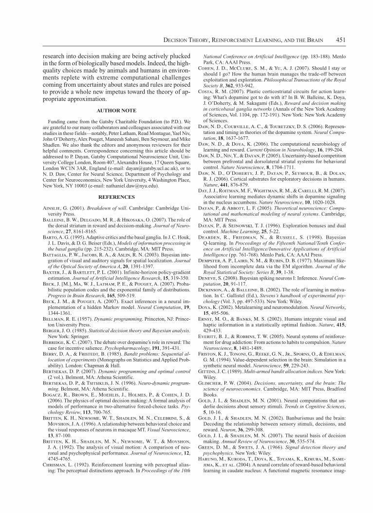
Decision Theory, reinforcemenT Learning, anD The Brain 451

National Conference on Artificial Intelligence (pp. 183­188). Menlo Park, CA: AAAI Press.

Cohen, J. D., McClure, S. M., & Yu, A. J. (2007). Should I stay or should I go? How the human brain manages the trade­off between exploitation and exploration. Philosophical Transactions of the Royal Society B, 362, 933­942.

Costa, R. M. (2007). Plastic corticostriatal circuits for action learn­ing: What’s dopamine got to do with it? In B. W. Balleine, K. Doya, J. O’Doherty, & M. Sakagami (Eds.), Reward and decision making in corticobasal ganglia networks (Annals of the New York Academy of Sciences, Vol. 1104, pp. 172­191). New York: New York Academy of Sciences.

Daw, N. D., Courville, A. C., & Touretzky, D. S. (2006). Represen­tation and timing in theories of the dopamine system. Neural Compu-tation, 18, 1637­1677.

Daw, N. D., & Doya, K. (2006). The computational neurobiology of learning and reward. Current Opinion in Neurobiology, 16, 199­204.

Daw, N. D., Niv, Y., & Dayan, P. (2005). Uncertainty­based competition between prefrontal and dorsolateral striatal systems for behavioral control. Nature Neuroscience, 8, 1704­1711.

Daw, N. D., O’Doherty, J. P., Dayan, P., Seymour, B., & Dolan, R. J. (2006). Cortical substrates for exploratory decisions in humans. Nature, 441, 876­879.

Day, J. J., Roitman, M. F., Wightman, R. M., & Carelli, R. M. (2007). Associative learning mediates dynamic shifts in dopamine signaling in the nucleus accumbens. Nature Neuroscience, 10, 1020­1028.

Dayan, P., & Abbott, L. F. (2005). Theoretical neuroscience: Compu-tational and mathematical modeling of neural systems. Cambridge, MA: MIT Press.

Dayan, P., & Sejnowski, T. J. (1996). Exploration bonuses and dual control. Machine Learning, 25, 5­22.

Dearden, R., Friedman, N., & Russell, S. (1998). Bayesian Q­ learning. In Proceedings of the Fifteenth National/Tenth Confer-ence on Artificial Intelligence/Innovative Applications of Artificial Intelligence (pp. 761­768). Menlo Park, CA: AAAI Press.

Dempster, A. P., Laird, N. M., & Rubin, D. B. (1977). Maximum like­lihood from incomplete data via the EM algorithm. Journal of the Royal Statistical Society: Series B, 39, 1­38.

Deneve, S. (2008). Bayesian spiking neurons I: Inference. Neural Com-putation, 20, 91­117.

Dickinson, A., & Balleine, B. (2002). The role of learning in motiva­tion. In C. Gallistel (Ed.), Stevens’s handbook of experimental psy-chology (Vol. 3, pp. 497­533). New York: Wiley.

Doya, K. (2002). Metalearning and neuromodulation. Neural Networks, 15, 495­506.

Ernst, M. O., & Banks, M. S. (2002). Humans integrate visual and haptic information in a statistically optimal fashion. Nature, 415, 429­433.

Everitt, B. J., & Robbins, T. W. (2005). Neural systems of reinforce­ment for drug addiction: From actions to habits to compulsion. Nature Neuroscience, 8, 1481­1489.

Friston, K. J., Tononi, G., Reeke, G. N., Jr., Sporns, O., & Edelman, G. M. (1994). Value­dependent selection in the brain: Simulation in a synthetic neural model. Neuroscience, 59, 229­243.

Gittins, J. C. (1989). Multi-armed bandit allocation indices. New York: Wiley.

Glimcher, P. W. (2004). Decisions, uncertainty, and the brain: The science of neuroeconomics. Cambridge, MA: MIT Press, Bradford Books.

Gold, J. I., & Shadlen, M. N. (2001). Neural computations that un­derlie decisions about sensory stim uli. Trends in Cognitive Sciences, 5, 10­16.

Gold, J. I., & Shadlen, M. N. (2002). Banburismus and the brain: Decoding the relationship between sensory stimuli, decisions, and reward. Neuron, 36, 299­308.

Gold, J. I., & Shadlen, M. N. (2007). The neural basis of decision making. Annual Review of Neuroscience, 30, 535­574.

Green, D. M., & Swets, J. A. (1966). Signal detection theory and psychophysics. New York: Wiley.

Haruno, M., Kuroda, T., Doya, K., Toyama, K., Kimura, M., Same-jima, K., et al. (2004). A neural correlate of reward­based behavioral learning in caudate nu cleus: A functional magnetic resonance imag­

research into decision making are being actively plucked in the form of biologically based models. Indeed, the high­quality choices made by animals and humans in environ­ments replete with extreme computational challenges coming from uncertainty about states and rules are poised to provide a whole new impetus toward the theory of ap­propriate approximation.

AUThOR NOTE

Funding came from the Gatsby Charitable Foundation (to P.D.). We are grateful to our many collab orators and colleagues associated with our studies in these fields—notably, Peter Latham, Read Montague, Yael Niv, John O’Doherty, Alex Pouget, Maneesh Sahani, Ben Seymour, and Mike Shadlen. We also thank the editors and anonymous reviewers for their helpful comments. Correspondence concerning this article should be addressed to P. Dayan, Gatsby Computational Neuroscience Unit, Uni­versity College London, Room 407, Alexandra House, 17 Queen Square, London WC1N 3AR, England (e­mail: dayan@gatsby.ucl.ac.uk), or to N. D. Daw, Center for Neural Science, Department of Psychology and Center for Neuroeconomics, New York University, 4 Washington Place, New York, NY 10003 (e­mail: nathaniel.daw@nyu.edu).

REFERENCES

Ainslie, G. (2001). Breakdown of will. Cambridge: Cambridge Uni­versity Press.

Balleine, B. W., Delgado, M. R., & Hikosaka, O. (2007). The role of the dorsal striatum in reward and decision­making. Journal of Neuro-science, 27, 8161­8165.

Barto, A. G. (1995). Adaptive critics and the basal ganglia. In J. C. Houk, J. L. Davis, & D. G. Beiser (Eds.), Models of information processing in the basal ganglia (pp. 215­232). Cambridge, MA: MIT Press.

Battaglia, P. W., Jacobs, R. A., & Aslin, R. N. (2003). Bayesian inte­gration of visual and auditory signals for spatial localization. Journal of the Optical Society of America A, 20, 1391­1397.

Baxter, J., & Bartlett, P. L. (2001). Infinite­horizon policy­gradient estimation. Journal of Artificial Intelligence Research, 15, 319­350.

Beck, J. [M.], Ma, W. J., Latham, P. E., & Pouget, A. (2007). Proba­bilistic population codes and the exponential family of distributions. Progress in Brain Research, 165, 509­519.

Beck, J. M., & Pouget, A. (2007). Exact inferences in a neural im­plementation of a hidden Markov model. Neural Computation, 19, 1344­1361.

Bellman, R. E. (1957). Dynamic programming. Princeton, NJ: Prince­ton University Press.

Berger, J. O. (1985). Statistical decision theory and Bayesian analysis. New York: Springer.

Berridge, K. C. (2007). The debate over dopamine’s role in reward: The case for incentive salience. Psychopharmacology, 191, 391­431.

Berry, D. A., & Fristedt, B. (1985). Bandit problems: Sequential al-location of experiments (Monographs on Statistics and Applied Prob­ability). London: Chapman & Hall.

Bertsekas, D. P. (2007). Dynamic programming and optimal control (2 vol.). Belmont, MA: Athena Scientific.

Bertsekas, D. P., & Tsitsiklis, J. N. (1996). Neuro-dynamic program-ming. Belmont, MA: Athena Scientific.

Bogacz, R., Brown, E., Moehlis, J., Holmes, P., & Cohen, J. D. (2006). The physics of optimal decision making: A formal analysis of models of performance in two­alternative forced­choice tasks. Psy-chology Review, 113, 700­765.

Britten, K. H., Newsome, W. T., Shadlen, M. N., Celebrini, S., & Movshon, J. A. (1996). A re lationship between behavioral choice and the visual responses of neurons in macaque MT. Visual Neuroscience, 13, 87­100.

Britten, K. H., Shadlen, M. N., Newsome, W. T., & Movshon, J. A. (1992). The analysis of visual motion: A comparison of neu­ronal and psychophysical performance. Journal of Neuroscience, 12, 4745­4765.

Chrisman, L. (1992). Reinforcement learning with perceptual alias­ing: The perceptual distinc tions approach. In Proceedings of the 10th

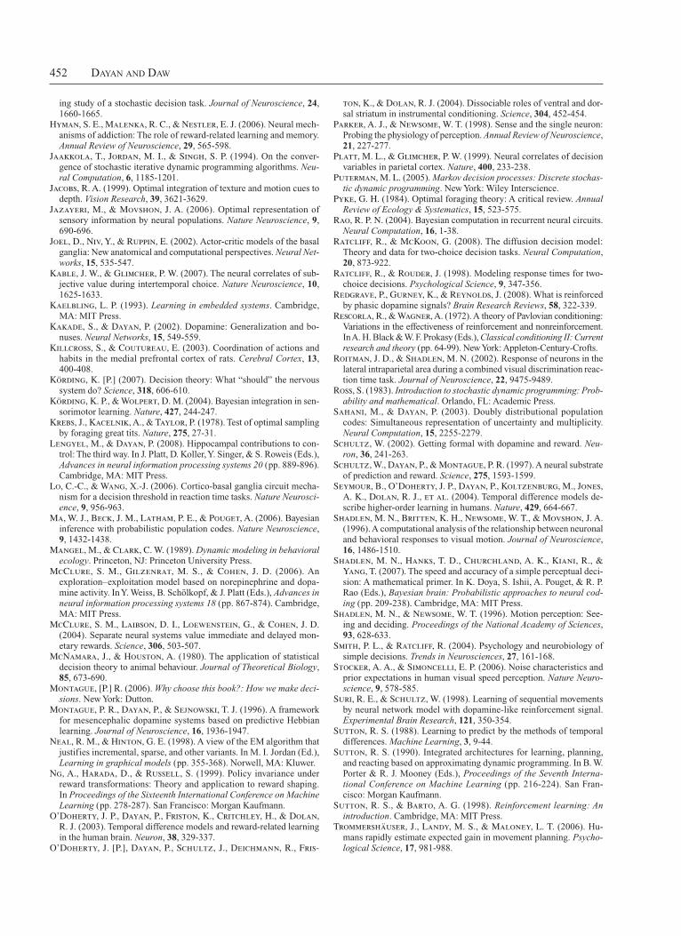
452 Dayan anD Daw

ton, K., & Dolan, R. J. (2004). Dissociable roles of ventral and dor­sal striatum in instrumental conditioning. Science, 304, 452­454.

Parker, A. J., & Newsome, W. T. (1998). Sense and the single neuron: Probing the physiology of perception. Annual Review of Neuroscience, 21, 227­277.

Platt, M. L., & Glimcher, P. W. (1999). Neural correlates of decision variables in parietal cortex. Nature, 400, 233­238.

Puterman, M. L. (2005). Markov decision processes: Discrete stochas-tic dynamic programming. New York: Wiley Interscience.

Pyke, G. H. (1984). Optimal foraging theory: A critical review. Annual Review of Ecology & Systematics, 15, 523­575.

Rao, R. P. N. (2004). Bayesian computation in recurrent neural circuits. Neural Computation, 16, 1­38.

Ratcliff, R., & McKoon, G. (2008). The diffusion decision model: Theory and data for two­choice decision tasks. Neural Computation, 20, 873­922.

Ratcliff, R., & Rouder, J. (1998). Modeling response times for two­choice decisions. Psychological Science, 9, 347­356.

Redgrave, P., Gurney, K., & Reynolds, J. (2008). What is reinforced by phasic dopamine signals? Brain Research Reviews, 58, 322­339.

Rescorla, R., & Wagner, A. (1972). A theory of Pavlovian conditioning: Variations in the effectiveness of reinforcement and nonreinforcement. In A. H. Black & W. F. Prokasy (Eds.), Classical conditioning II: Current research and theory (pp. 64­99). New York: Appleton­Century­Crofts.

Roitman, J. D., & Shadlen, M. N. (2002). Response of neurons in the lateral intraparietal area during a combined visual discrimination reac­tion time task. Journal of Neuroscience, 22, 9475­9489.

Ross, S. (1983). Introduction to stochastic dynamic programming: Prob-ability and mathematical. Orlando, FL: Academic Press.

Sahani, M., & Dayan, P. (2003). Doubly distributional population codes: Simultaneous represen tation of uncertainty and multiplicity. Neural Computation, 15, 2255­2279.

Schultz, W. (2002). Getting formal with dopamine and reward. Neu-ron, 36, 241­263.

Schultz, W., Dayan, P., & Montague, P. R. (1997). A neural substrate of prediction and reward. Science, 275, 1593­1599.

Seymour, B., O’Doherty, J. P., Dayan, P., Koltzenburg, M., Jones, A. K., Dolan, R. J., et al. (2004). Temporal difference models de­scribe higher­order learning in humans. Nature, 429, 664­667.

Shadlen, M. N., Britten, K. H., Newsome, W. T., & Movshon, J. A. (1996). A computational analysis of the relationship between neuronal and behavioral responses to visual motion. Journal of Neuroscience, 16, 1486­1510.

Shadlen, M. N., Hanks, T. D., Churchland, A. K., Kiani, R., & Yang, T. (2007). The speed and accuracy of a simple perceptual deci­sion: A mathematical primer. In K. Doya, S. Ishii, A. Pouget, & R. P. Rao (Eds.), Bayesian brain: Probabilistic approaches to neural cod-ing (pp. 209­238). Cambridge, MA: MIT Press.

Shadlen, M. N., & Newsome, W. T. (1996). Motion perception: See­ing and deciding. Proceedings of the National Academy of Sciences, 93, 628­633.

Smith, P. L., & Ratcliff, R. (2004). Psychology and neurobiology of simple decisions. Trends in Neurosciences, 27, 161­168.

Stocker, A. A., & Simoncelli, E. P. (2006). Noise characteristics and prior expectations in human visual speed perception. Nature Neuro-science, 9, 578­585.

Suri, R. E., & Schultz, W. (1998). Learning of sequential movements by neural network model with dopamine­like reinforcement signal. Experimental Brain Research, 121, 350­354.

Sutton, R. S. (1988). Learning to predict by the methods of temporal differences. Machine Learning, 3, 9­44.

Sutton, R. S. (1990). Integrated architectures for learning, planning, and reacting based on approximating dynamic programming. In B. W. Porter & R. J. Mooney (Eds.), Proceedings of the Seventh Interna-tional Conference on Machine Learning (pp. 216­224). San Fran­cisco: Morgan Kaufmann.

Sutton, R. S., & Barto, A. G. (1998). Reinforcement learning: An introduction. Cambridge, MA: MIT Press.

Trommershäuser, J., Landy, M. S., & Maloney, L. T. (2006). Hu­mans rapidly estimate expected gain in movement planning. Psycho-logical Science, 17, 981­988.

ing study of a stochastic decision task. Journal of Neuroscience, 24, 1660­1665.

Hyman, S. E., Malenka, R. C., & Nestler, E. J. (2006). Neural mech­anisms of addiction: The role of reward­related learning and memory. Annual Review of Neuroscience, 29, 565­598.

Jaakkola, T., Jordan, M. I., & Singh, S. P. (1994). On the conver­gence of stochastic iterative dynamic programming algorithms. Neu-ral Computation, 6, 1185­1201.

Jacobs, R. A. (1999). Optimal integration of texture and motion cues to depth. Vision Research, 39, 3621­3629.

Jazayeri, M., & Movshon, J. A. (2006). Optimal representation of sensory information by neural populations. Nature Neuroscience, 9, 690­696.

Joel, D., Niv, Y., & Ruppin, E. (2002). Actor­critic models of the basal ganglia: New anatomical and computational perspectives. Neural Net-works, 15, 535­547.

Kable, J. W., & Glimcher, P. W. (2007). The neural correlates of sub­jective value during intertem poral choice. Nature Neuroscience, 10, 1625­1633.

Kaelbling, L. P. (1993). Learning in embedded systems. Cambridge, MA: MIT Press.

Kakade, S., & Dayan, P. (2002). Dopamine: Generalization and bo­nuses. Neural Networks, 15, 549­559.

Killcross, S., & Coutureau, E. (2003). Coordination of actions and habits in the medial prefrontal cortex of rats. Cerebral Cortex, 13, 400­408.

Körding, K. [P.] (2007). Decision theory: What “should” the nervous system do? Science, 318, 606­610.

Körding, K. P., & Wolpert, D. M. (2004). Bayesian integration in sen­sorimotor learning. Nature, 427, 244­247.

Krebs, J., Kacelnik, A., & Taylor, P. (1978). Test of optimal sampling by foraging great tits. Nature, 275, 27­31.

Lengyel, M., & Dayan, P. (2008). Hippocampal contributions to con­trol: The third way. In J. Platt, D. Koller, Y. Singer, & S. Roweis (Eds.), Advances in neural information processing systems 20 (pp. 889­896). Cambridge, MA: MIT Press.

Lo, C.-C., & Wang, X.-J. (2006). Cortico­basal ganglia circuit mecha­nism for a decision threshold in reaction time tasks. Nature Neurosci-ence, 9, 956­963.

Ma, W. J., Beck, J. M., Latham, P. E., & Pouget, A. (2006). Bayesian inference with probabilistic population codes. Nature Neuroscience, 9, 1432­1438.

Mangel, M., & Clark, C. W. (1989). Dynamic modeling in behavioral ecology. Princeton, NJ: Princeton University Press.

McClure, S. M., Gilzenrat, M. S., & Cohen, J. D. (2006). An exploration– exploitation model based on norepinephrine and dopa­mine activity. In Y. Weiss, B. Schölkopf, & J. Platt (Eds.), Advances in neural information processing systems 18 (pp. 867­874). Cambridge, MA: MIT Press.

McClure, S. M., Laibson, D. I., Loewenstein, G., & Cohen, J. D. (2004). Separate neural systems value immediate and delayed mon­etary rewards. Science, 306, 503­507.

McNamara, J., & Houston, A. (1980). The application of statistical decision theory to animal behaviour. Journal of Theoretical Biology, 85, 673­690.

Montague, [P.] R. (2006). Why choose this book?: How we make deci-sions. New York: Dutton.

Montague, P. R., Dayan, P., & Sejnowski, T. J. (1996). A framework for mesencephalic dopamine systems based on predictive Hebbian learning. Journal of Neuroscience, 16, 1936­1947.

Neal, R. M., & Hinton, G. E. (1998). A view of the EM algorithm that justifies incremental, sparse, and other variants. In M. I. Jordan (Ed.), Learning in graphical models (pp. 355­368). Norwell, MA: Kluwer.

Ng, A., Harada, D., & Russell, S. (1999). Policy invariance under reward transformations: The ory and application to reward shaping. In Proceedings of the Sixteenth International Conference on Machine Learning (pp. 278­287). San Francisco: Morgan Kaufmann.

O’Doherty, J. P., Dayan, P., Friston, K., Critchley, H., & Dolan, R. J. (2003). Temporal difference models and reward­related learning in the human brain. Neuron, 38, 329­337.

O’Doherty, J. [P.], Dayan, P., Schultz, J., Deichmann, R., Fris-

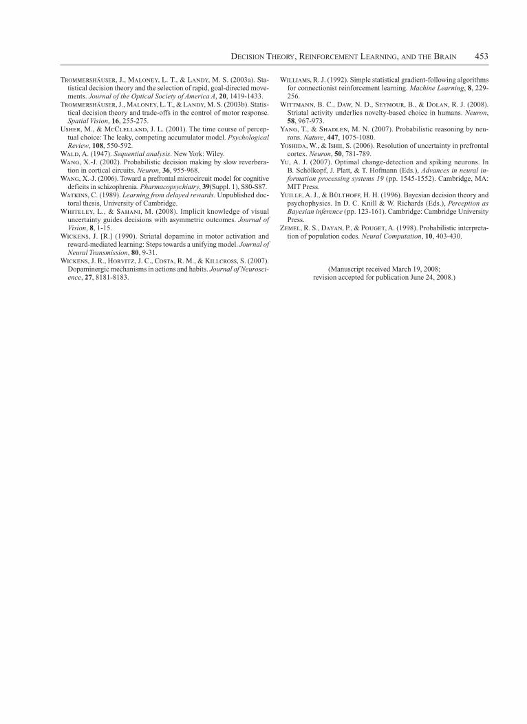
Decision Theory, reinforcemenT Learning, anD The Brain 453

Williams, R. J. (1992). Simple statistical gradient­following algorithms for connectionist reinforcement learning. Machine Learning, 8, 229­256.

Wittmann, B. C., Daw, N. D., Seymour, B., & Dolan, R. J. (2008). Striatal activity underlies novelty­based choice in humans. Neuron, 58, 967­973.

Yang, T., & Shadlen, M. N. (2007). Probabilistic reasoning by neu­rons. Nature, 447, 1075­1080.

Yoshida, W., & Ishii, S. (2006). Resolution of uncertainty in prefrontal cortex. Neuron, 50, 781­789.

Yu, A. J. (2007). Optimal change­detection and spiking neurons. In B. Schölkopf, J. Platt, & T. Hofmann (Eds.), Advances in neural in-formation processing systems 19 (pp. 1545­1552). Cambridge, MA: MIT Press.

Yuille, A. J., & Bülthoff, H. H. (1996). Bayesian decision theory and psychophysics. In D. C. Knill & W. Richards (Eds.), Perception as Bayesian inference (pp. 123­161). Cambridge: Cambridge University Press.

Zemel, R. S., Dayan, P., & Pouget, A. (1998). Probabilistic interpreta­tion of population codes. Neural Computation, 10, 403­430.

(Manuscript received March 19, 2008; revision accepted for publication June 24, 2008.)

Trommershäuser, J., Maloney, L. T., & Landy, M. S. (2003a). Sta­tistical decision theory and the selection of rapid, goal­directed move­ments. Journal of the Optical Society of America A, 20, 1419­1433.

Trommershäuser, J., Maloney, L. T., & Landy, M. S. (2003b). Statis­tical decision theory and trade­offs in the control of motor response. Spatial Vision, 16, 255­275.

Usher, M., & McClelland, J. L. (2001). The time course of percep­tual choice: The leaky, competing accumulator model. Psychological Review, 108, 550­592.

Wald, A. (1947). Sequential analysis. New York: Wiley.Wang, X.-J. (2002). Probabilistic decision making by slow reverbera­

tion in cortical circuits. Neuron, 36, 955­968.Wang, X.-J. (2006). Toward a prefrontal microcircuit model for cognitive

deficits in schizophrenia. Pharmacopsychiatry, 39(Suppl. 1), S80­S87.Watkins, C. (1989). Learning from delayed rewards. Unpublished doc­

toral thesis, University of Cambridge.Whiteley, L., & Sahani, M. (2008). Implicit knowledge of visual

uncertainty guides decisions with asymmetric outcomes. Journal of Vision, 8, 1­15.

Wickens, J. [R.] (1990). Striatal dopamine in motor activation and reward­ mediated learning: Steps towards a unifying model. Journal of Neural Transmission, 80, 9­31.

Wickens, J. R., Horvitz, J. C., Costa, R. M., & Killcross, S. (2007). Dopaminergic mechanisms in actions and habits. Journal of Neurosci-ence, 27, 8181­8183.