1

Use Decision Trees to Make Important Project Decisions1

By David T. Hulett, Ph.D.

ABSTRACT— a large part of the risk management process involves looking into the future, trying to understand what might happen and whether it matters to an important decision we need to make. An important quantitative technique which has been neglected in recent years – decision trees – is enjoying something of a revival. Decision trees help organizations choose between alternative courses of action, for instance project management strategies, when the results of such actions are uncertain. The decision tree technique can be applied to many different uncertain situations. For example:

Should we use the low-price bidder when delivery and quality uncertain?

Should we adopt a state-of-the-art technology if we may not know how to do this? This Recommended Practice looks at two different approaches to making the decision:

Maximize expected monetary value, which is a hallmark of a risk-neutral organization

Maximize expected utility, which is the appropriate measure of merit for a risk-averse or even a risk-seeking organization

We use sensitivity analysis to look at the importance of data accuracy in decision-making, whether it is worth gathering more data, which depends on the accuracy of the existing data and whether a reasonable variation in the numbers will actually change the decision. Finally, continuous distributions of the uncertain variables usually approximate reality better than selecting and representing alternative outcomes using a limited number of discrete outcomes. Uncertain future uncertain outcomes can be represented by the use of Monte Carlo simulations of continuous distributions. This paper describes these two approaches and compares their results using simple decision models.

1 This draws some material from a paper written by David Hulett and David Hillson [2]

2

Introduction A large part of the risk management process involves looking into the future, trying to understand what might happen and whether it matters to the success of the project. Making this process difficult is the uncertainty of results, particularly results of key decisions that are made early in the project when alternatives are available. An important quantitative technique which has been neglected in recent years – decision trees – is enjoying something of a revival. Decision trees help organizations choose between alternative courses of action, for instance project management strategies, when the results of such actions are uncertain. At heart the decision tree technique for making decisions in the presence of uncertainty is really quite simple, and can be applied to many different uncertain situations. For example:

Should we use the low-price bidder? Is there an analytic rationale for choosing a high-bidding company that provides more reliable delivery?

Should we adopt a state-of-the-art technology? What are the risks that might occur, including that we may not know how to implement it?

Should we construct a greenfield plant or expand an existing plant? What levels of profit can we expect from each alternative, and how likely are they to occur?

While making many decisions is difficult, the particular difficulty of making these decisions is that the results of choosing the alternatives available may be uncertain, ambiguous, unknown or even unknowable. Decision tree methods can help make decisions when the results are not known with certainty by comparing their expected value or expected utility to the organization. The term “expected value” or “expected utility” imply that there are alternative outcomes that can be described only with probabilistic statements. It may be easy to make a decision rule for which the results are known with certainty, such as: “Take the choice that yields the highest net present value (NPV).” But we need a more complex rule to value outcomes and make decisions when the NPV depends on factors, such as future performance of a contractor or the state of the economy, that are not known with certainty. This paper illustrates the difference in the methodology, and often of the decision taken, by using expected monetary if the organization is risk neutral or expected utility if it is risk averse. With uncertainty, we will generally make the decision which has the:

Highest expected value (risk neutral organizations), or

Highest expected utility (risk averse organizations). The calculation of these values of merit is described in this paper using simple examples and a spreadsheet add-in software tool, Precision Tree2, which is easily available for this purpose. This paper distinguishes between those organizations that are risk neutral and those that are risk averse.

2 Precision Tree® is a software product of Palisade Corporation. There are several other similar decision analysis

software packages.

3

A risk-neutral organization values gains and losses by their dollar value no matter how large the gain or loss is. A loss of $1 million is equally as bad as a gain of $1 million is good. The risk neutral organization evaluates alternative decisions using expected monetary value, calculated by multiplying the value of each possible result by its probability of occurring and adding the probability-weighted values of all possible results. This is equivalent to applying a linear utility function. Generally if the value of a decision calculated this way is not large enough the organization will not do it.3

A risk-averse organization has a stronger aversion to losses of a given value than attraction to gains of the same value. They will tend to avoid decisions that have a possible loss result even if there is an equivalent possibility of equivalent, or sometimes even greater, gains with that decision. Risk-averse organizations typically use expected utility and implement a more complex non-linear utility function to value outcomes. These may be smaller organizations that have one or only a few projects. If one project fails the company will be severely affected.

Many decisions have uncertain outcomes in risky projects, and we often need to make a decision even if we do not know for sure how it will turn out. These can be very important decisions for the project, and making them using correct decision-making discipline that includes the probability of alternative results increases the possibility of project success. Simple but Crucial Decision with Uncertain Outcomes We can illustrate decision tree analysis by considering a common decision faced on a project. We are the prime contractor and there is a penalty in our contract with the customer that depends on how many days we deliver late. We need to decide which contractor to use for a critical activity. Our aim is to minimize our expected cost, including the cost of the contract with the subcontractor and the penalty if we do not achieve an on-time and on-scope delivery. It is often difficult to argue for using the higher-priced contractor, even if that one is known to deliver reliably on time. Of course the lower-bidding contractor also promises a successful delivery, although we suspect that he cannot do so reliably. Even the high-priced contractor may deliver late, but that is relatively unlikely. Structure the Decision Tree A rigorous analysis of this decision using a simplified decision tree structure that minimizes our expected cost is shown below:

3 There are many other factors such as strategy, competitive advantage, customer relationships, market share and

reputation that could cause a risk-neutral organization to make a decision to do something with negative expected

value. We are not considering those factors in this paper.

4

One contractor that we have not worked with before presents a lower-cost ($120,000) bid. We estimate however that there is a 60% chance that this contractor will be late incurring a penalty of $50,000.

The higher-cost contractor bids $140,000. We know this contractor and assess that it poses only a 30% chance of being late, with a late penalty of $30,000 at that.

We need to know if there is any benefit to using the higher-cost subcontractor. We suspect that any benefit may lie in the greater reliability of performance and avoidance of penalty payments we expect, but we need to check to see if this is true. We need to know if that benefit is enough to make up for the difference in bids between $140,000 and $120,000. Of course, both we and our customer need to be convinced of the benefit since, if the analysis shows a benefit to using the expensive but reliable subcontractor the project baseline budget will be higher. A formal analysis using decision trees will ascertain if there is a benefit, and will also document it for the customer and any potential challenge from the contractor not chosen. The steps we need to implement are as follows:

Identify the objective. Some trees will be built to make decisions to maximize value, such as Net Present Value or profit. In this example we are trying to find the lowest-cost contractor so we are trying to make decisions that minimize cost given uncertain results of our decisions.

Identify the major decisions to be made, in this case to engage one or the other contractor. In the decision tree this is called a decision node. We will have to live with this decision for the duration of the project.

Identify the major uncertainties, in this case delivering later than agreed in the contract. Uncertainties are specified in event nodes that relate to the consequences and their probabilities.

Construct the structure of the decision and all of its (main) consequences. Because each decision or event node has at least two alternatives, the structure of the decision looks like a tree, typically placed on its side with the root on the left and the branches on the right.

Solve the tree, in this case to find the lowest cost subcontracting strategy. We show a simple model in Figure 1, but there are potentially many branches.

5

Figure 1 - Contractor Decision - Basic Decision Tree Structure

Estimate Values such as Costs and Returns Estimate the costs (and benefits if relevant to the decision being made) of each alternative decision. This is a task of some importance since the final result of the decision tree analysis will depend on the realism of these comparative estimates. Engineering estimates or estimating using comparable data from past projects should be used. In this case the implication of being late is known and, for this example, we assume that the duration is also known. These are shown on Figure 2.

6

Figure 2 - Adding Costs (and benefits if appropriate) to the Decision Tree Rolling Forward to Determine Path Values To calculate the value of the project for each path start at the decision node on the left-hand side with the first decision and adding / subtracting as appropriate all the values up to and including to the final branch tip on the right as if each of the decisions along the path were taken and each event along the branch occurred. This action is called “rolling forward.” For example, taking the top-most branch shown in Figure 2, the lower bidder bids $120,000 and if they are late a reasonable estimate of penalties added by our customer is $50,000 for a total cost to us of $170,000. This rolling forward calculation of the four possible path values is shown in Figure 3.

Figure 3 - Contractor Decision – Rolling Forward to find the Path Values

Add Probabilities for the Uncertain Events To identify the correct decision and its value (to “solve the tree”) we need to estimate some additional data, namely the probability of each possible uncertain outcome. Estimating these probabilities is not as easy as it might appear, since there are often no useful databases from which to extract the data. Expert judgment is usually required and that judgment may be poorly-informed or biased. During data interviews of several subject matter experts (SMEs) several different estimates of probability may be gathered. These must be reconciled. Probabilities are added in Figure 4.

7

Figure 4 - Adding Probabilities for Uncertain Outcomes

Solve the Tree by Folding Back To solve the tree we must calculate the value of each node – including both chance nodes and decision nodes. We start with the path values at the far right-hand end of the tree. Moving from the right to the left we calculate the value of each node as it is encountered. This process is called “folding back” the tree. The rules for finding the values of the chance and decision nodes are:

Chance Node value: The value of each chance node is found by multiplying the values of the uncertain alternatives by their probabilities of occurring and sum the results. This value is known as Expected Monetary Value (EMV). [2]

Decision Node value: Since we are trying to minimize the cost of this subcontract, the value of a decision node is, in this case, the lowest cost value of the succeeding branches leading from that node.

In Figure 5 we see that the value of the chance node for the expensive-but-reliable subcontractor is -$149,000. That is a lower cost than that for using the low cost but risky contractor which is calculated at -$150,000. When comparing the two alternatives and considering their assessed ability to deliver on time, the Reliable High Bidder is shown to be the lowest-cost selection. With this analysis behind us, we go to the customer and propose hiring the $140,000 subcontractor.

8

Figure 5 - Contractor Decision - Folding back to find the EMV

The “folding back” calculations for our simple example are as follows:

For the “Low Bidder but Risky” alternative 1. Multiply -$170,000 by 60% for -$102,000 2. Multiply -$120,000 by 40% for -$48,000 3. Add these numbers (- $102,000 - $48,000) for - $150,000. This is the Expected

Cost of this option, since it is 60% likely that the low bidder will be late causing penalty cost of $50,000.

For the Reliable High Bidder 1. Multiply -$170,000 x 30% for - $51,000 2. Multiply -$140,000 x 70% = - $98,000 3. Add the results (- $51,000 and - $98,000) for - $149,000

In the Contractor Decision case there is only one decision node, the original one. The alternatives are:

(1) Low Bidder but Risky at -$150,000 (2) Reliable High Bidder at -$149,000.

The reliable high bidder has the edge here and is actually expected to cost less for the project because:

A greater on-time reliability

Shorter delayed delivery, if that unlikely event occurs. The value of the process is to improve on a simple comparison of nominal bids by evaluating the values corrected for, or incorporating in, their uncertainty. Sensitivity Analysis to Find Important Data Elements that may Change the Decision

9

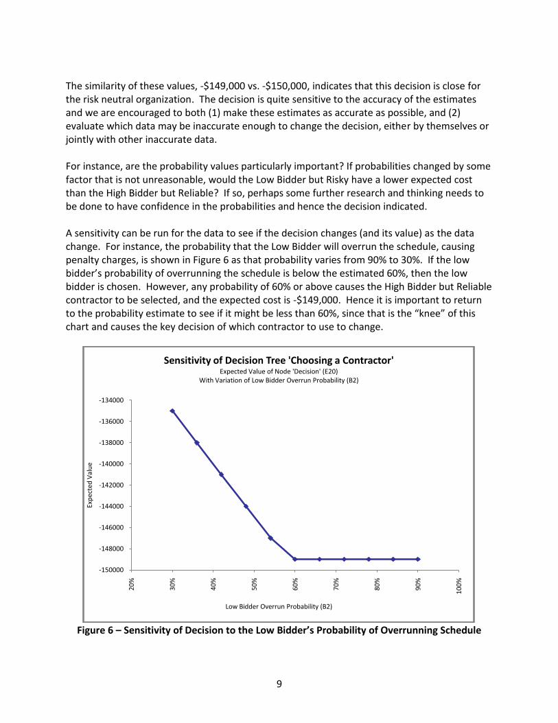
The similarity of these values, -$149,000 vs. -$150,000, indicates that this decision is close for the risk neutral organization. The decision is quite sensitive to the accuracy of the estimates and we are encouraged to both (1) make these estimates as accurate as possible, and (2) evaluate which data may be inaccurate enough to change the decision, either by themselves or jointly with other inaccurate data. For instance, are the probability values particularly important? If probabilities changed by some factor that is not unreasonable, would the Low Bidder but Risky have a lower expected cost than the High Bidder but Reliable? If so, perhaps some further research and thinking needs to be done to have confidence in the probabilities and hence the decision indicated. A sensitivity can be run for the data to see if the decision changes (and its value) as the data change. For instance, the probability that the Low Bidder will overrun the schedule, causing penalty charges, is shown in Figure 6 as that probability varies from 90% to 30%. If the low bidder’s probability of overrunning the schedule is below the estimated 60%, then the low bidder is chosen. However, any probability of 60% or above causes the High Bidder but Reliable contractor to be selected, and the expected cost is -$149,000. Hence it is important to return to the probability estimate to see if it might be less than 60%, since that is the “knee” of this chart and causes the key decision of which contractor to use to change.

Figure 6 – Sensitivity of Decision to the Low Bidder’s Probability of Overrunning Schedule

-150000

-148000

-146000

-144000

-142000

-140000

-138000

-136000

-134000

20

%

30

%

40

%

50

%

60

%

70

%

80

%

90

%

10

0%

Exp

ecte

d V

alu

e

Low Bidder Overrun Probability (B2)

Sensitivity of Decision Tree 'Choosing a Contractor'Expected Value of Node 'Decision' (E20)

With Variation of Low Bidder Overrun Probability (B2)

10

Decision Tree Analysis for the Risk-Averse Organization Most organizations realize that they do not do the same project many times over and over again. They perform the project only once and therefore have only one chance to “get it right.” Also, the organization may be particularly sensitive to losses, for instance if they are small or if the project is for their best customer. Knowing this, they may see problems with relying on the average or expected result represented by the EMV to make the correct decision and to value the project:

There is no assurance that their specific project will have the average result.

They may not have many other projects in process so they cannot rely on the average.

They may be more concerned with the possibility of failure if the customer is crucial to their future business.

It is at this point that we need to realize that decision tree analysis methodology and the tools that implement it do not require the use of EMV or E (MV). Decision trees can be solved based on an expected utility, or E (U), of the project to the performing organization. There is no requirement that utility is measured by expected dollars. In fact, non-linear utility functions can be substituted for linear EMV in most decision tree software packages, and E (U) is then substituted for E (MV) as the decision criterion. There is a trick to analyzing the E(U) of the choices, of course. How do we know the organization’s utility function? We know how to calculate the EMV of alternative bets and their values: multiply the values of the alternative bets by their probabilities and sum those results across all possible alternative bets. However, if utility is not equal to the economic value of the outcome, how do we identify the utility of each scenario to the organization in order to take its expected value? We substitute utility for value and decide on E (U) rather than on E (MV). Risk Averse Organizations using Expected Utility Many, if not most, organizations are cautious in situations where they think they might be vulnerable to losses. These organizations may shy away from project alternatives which, if they were to fail, would expose the organization to significant down-side results, even if the alternatives also offer a possibility of comparably large up-side results and success. This behavior might be called “risk-averse.” Companies exhibiting risk aversion can be perfectly rational given their circumstances but they do not succeed in risk-taking industries. Decisions made by risk-averse organizations’ tend to be best represented by models that maximize their E (U) rather than EMV. We can then build a utility function that may give serious negative utility to the possibility of large losses, in comparison to the serious positive utility to the possibility of comparable large monetary gain. Most decision tree software allows

11

the user to design a utility function that reflects the organization’s degree of aversion to large losses.4 The risk-averse organization often perceives a greater aversion to losses from failure of the project than benefit from a similar-size gain from project success. For this organization, the fear of losing $1 million far overweighs the benefit of gaining $1 million. Risk-averse organizations are not indifferent between the two possible outcomes – they avoid decisions that have significant possibilities of bad results, even if that means they “pass” on opportunities for seriously good results. The preference for avoiding large losses is quite strong and may outweigh the benefit of gaining the same amount or more. A similar approach is in [3]. The comparison of the way risk-neutral E (MV) decision-making and risk averse (E (U)) decision-making organizations is shown in Figure 7.

Figure 7 - Different Approaches to Assessing the Value of the Benefit or Loss

Figure 7 – Risk-Neutral and Risk-Averse Utility Curves Figure 7 shows two organizations’ evaluation of the benefit or loss from different results.

The straight line (linear utility) represents the way a risk-neutral organization would value the benefit or loss. Notice that the utility (vertical or Y-axis) value associated with the benefit of $100 (on the horizontal or X-axis) is $100. Conversely, the value to this

4 We are using Precision Tree® from Palisade for these illustrations.

Utility Function

-500.00

-400.00

-300.00

-200.00

-100.00

0.00

100.00

200.00

-200 -150 -100 -50 0 50 100

Benefit or Loss

Risk

Averse

Risk

Neutral

Utility to the Organization

12

organization that is associated with a loss of $100 on the X-axis is minus $100 on the Y-axis. For this organization, the value of benefit and loss is simply the dollar amount of that benefit or loss. A 50-50 chance of winning or losing $100 has an EMV of zero. The risk neutral organization feels this is neither attractive nor unattractive.

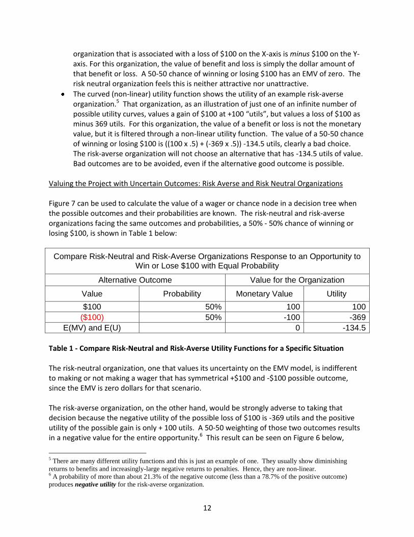
The curved (non-linear) utility function shows the utility of an example risk-averse organization.5 That organization, as an illustration of just one of an infinite number of possible utility curves, values a gain of $100 at +100 “utils”, but values a loss of $100 as minus 369 utils. For this organization, the value of a benefit or loss is not the monetary value, but it is filtered through a non-linear utility function. The value of a 50-50 chance of winning or losing $100 is ((100 x .5) + (-369 x .5)) -134.5 utils, clearly a bad choice. The risk-averse organization will not choose an alternative that has -134.5 utils of value. Bad outcomes are to be avoided, even if the alternative good outcome is possible.

Valuing the Project with Uncertain Outcomes: Risk Averse and Risk Neutral Organizations Figure 7 can be used to calculate the value of a wager or chance node in a decision tree when the possible outcomes and their probabilities are known. The risk-neutral and risk-averse organizations facing the same outcomes and probabilities, a 50% - 50% chance of winning or losing $100, is shown in Table 1 below:

Compare Risk-Neutral and Risk-Averse Organizations Response to an Opportunity to Win or Lose $100 with Equal Probability

Alternative Outcome Value for the Organization

Value Probability Monetary Value Utility

$100 50% 100 100

($100) 50% -100 -369

E(MV) and E(U) 0 -134.5

Table 1 - Compare Risk-Neutral and Risk-Averse Utility Functions for a Specific Situation The risk-neutral organization, one that values its uncertainty on the EMV model, is indifferent to making or not making a wager that has symmetrical +$100 and -$100 possible outcome, since the EMV is zero dollars for that scenario. The risk-averse organization, on the other hand, would be strongly adverse to taking that decision because the negative utility of the possible loss of $100 is -369 utils and the positive utility of the possible gain is only + 100 utils. A 50-50 weighting of those two outcomes results in a negative value for the entire opportunity.6 This result can be seen on Figure 6 below,

5 There are many different utility functions and this is just an example of one. They usually show diminishing

returns to benefits and increasingly-large negative returns to penalties. Hence, they are non-linear. 6 A probability of more than about 21.3% of the negative outcome (less than a 78.7% of the positive outcome)

produces negative utility for the risk-averse organization.

13

where the result is found on the straight line between the value of utility at +$100 and -$100 on the X axis that matches the relative probabilities:

Figure 8 - Value of a 50-50 Outcome for Risk-Neutral and Risk-Averse Organizations

Other combinations of values and probabilities can be evaluated using the chart. Table 2 shows alternative wagers or bets (ventures with uncertain outcomes) that have the same value of outcome but differ as to the probability of each. These would show as different points on the utility curves, including that a 20% possibility of the loss outcome has a marginally positive expected utility, though a large $60 EMV.

Compare Risk-Neutral E(monetary Value) and Risk-Averse E(utility) Calculations by Probability of Occurring

Pr(100) Pr(-100) E(utility) E(MV)

80% 20% 6 60

60% 40% -88 20

40% 60% -182 -20

20% 80% -275 -60

Table 2 - Expected Utility and EMV for Different Probabilities of a Wager Note from the results of Table 2, the Risk-Averse organization would barely accept the wager if it had an 80% chance of success, and it would reject the wager if it has “only” a 60% chance of success. Over a fair range of relative probabilities, from a probability of loss of 50% to probability of 79%, the two organizations’ decisions will be different. A decision analyst needs to know which utility function applies to his or her organization in order to make recommendations that are consistent with the organization’s attitudes toward risk.

Utility Function

0

-135

-500.00

-400.00

-300.00

-200.00

-100.00

0.00

100.00

200.00

-200 -150 -100 -50 0 50 100

Benefit or Loss

Risk

Averse

Risk

Neutral

Value of

Bet

Utility to the

Organization

14

Comparison of Risk-Neutral and Risk-Averse Decisions – Simple Example A personal example that may be familiar to all is the following example. A person will be asked to play a game with a risk of gain and loss and its probabilities. Will it accept that project or not? In the figure that follows (Figure 9) the risk-neutral person is offered a game that costs $20 to flip a coin once, with a $50 value if the coin lands heads and no payout if the coin lands tails.

Figure 9 - A Risk-Neutral Person Accepts this Project because its EMV is +$5

In Figure 10, below, the costs and rewards are larger, but the probabilities are the same and the expected value is still + $5. The risk-neutral person will take this wager as well, even though there is a 50% chance of losing $470 (the entry fee and the $450 penalty for “tails”).

Figure 10 - A Risk-Neutral Person Accepts this Project because its EMV is +$5

Apply the risk-averse person’s utility function to each of these examples to understand how the utility function works with the data to help make the decision. In the first risk-averse example the small payoff for “heads” and zero for “tails” is used. There are some risk-averse

15

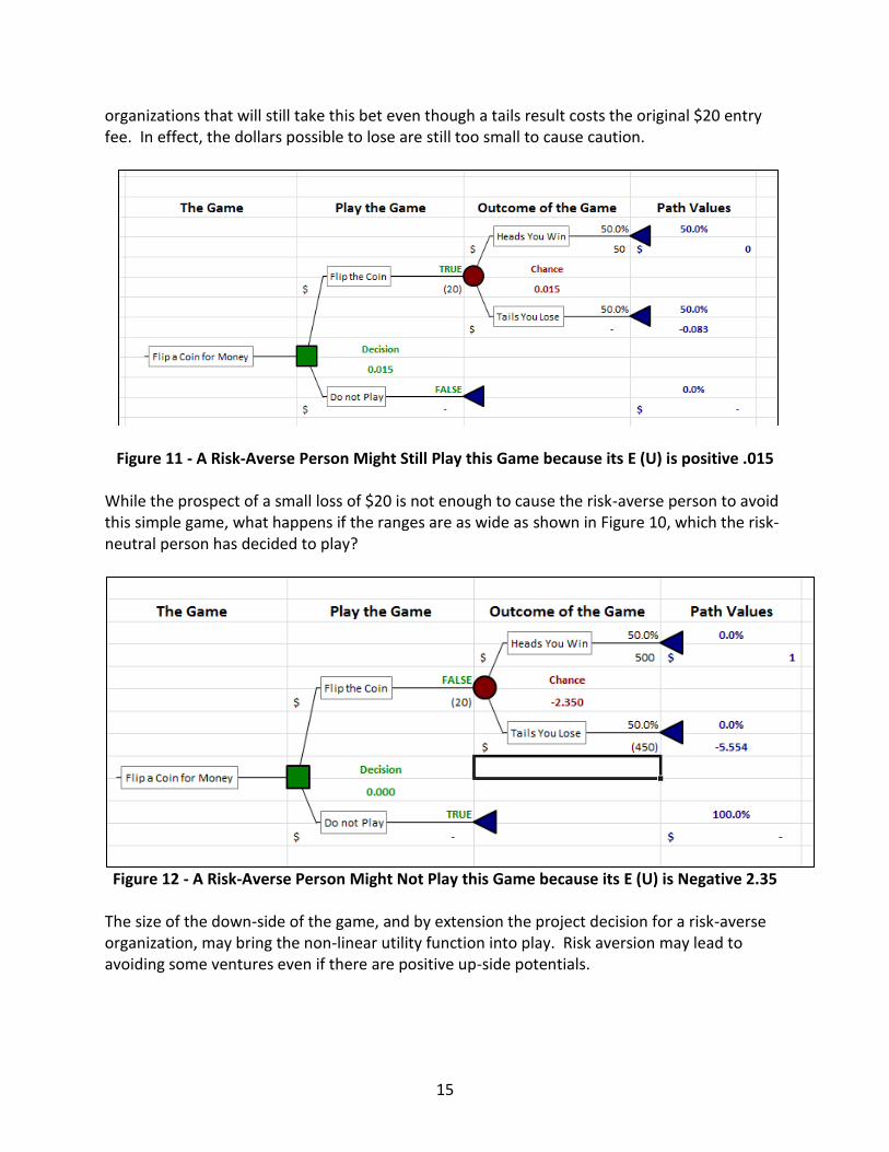
organizations that will still take this bet even though a tails result costs the original $20 entry fee. In effect, the dollars possible to lose are still too small to cause caution.

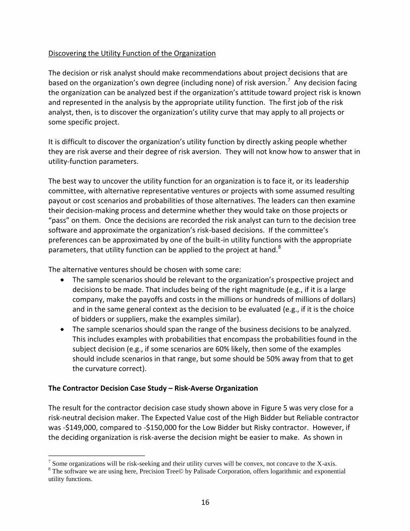
Figure 11 - A Risk-Averse Person Might Still Play this Game because its E (U) is positive .015 While the prospect of a small loss of $20 is not enough to cause the risk-averse person to avoid this simple game, what happens if the ranges are as wide as shown in Figure 10, which the risk-neutral person has decided to play?

Figure 12 - A Risk-Averse Person Might Not Play this Game because its E (U) is Negative 2.35

The size of the down-side of the game, and by extension the project decision for a risk-averse organization, may bring the non-linear utility function into play. Risk aversion may lead to avoiding some ventures even if there are positive up-side potentials.

16

Discovering the Utility Function of the Organization The decision or risk analyst should make recommendations about project decisions that are based on the organization’s own degree (including none) of risk aversion.7 Any decision facing the organization can be analyzed best if the organization’s attitude toward project risk is known and represented in the analysis by the appropriate utility function. The first job of the risk analyst, then, is to discover the organization’s utility curve that may apply to all projects or some specific project. It is difficult to discover the organization’s utility function by directly asking people whether they are risk averse and their degree of risk aversion. They will not know how to answer that in utility-function parameters. The best way to uncover the utility function for an organization is to face it, or its leadership committee, with alternative representative ventures or projects with some assumed resulting payout or cost scenarios and probabilities of those alternatives. The leaders can then examine their decision-making process and determine whether they would take on those projects or “pass” on them. Once the decisions are recorded the risk analyst can turn to the decision tree software and approximate the organization’s risk-based decisions. If the committee’s preferences can be approximated by one of the built-in utility functions with the appropriate parameters, that utility function can be applied to the project at hand.8 The alternative ventures should be chosen with some care:

The sample scenarios should be relevant to the organization’s prospective project and decisions to be made. That includes being of the right magnitude (e.g., if it is a large company, make the payoffs and costs in the millions or hundreds of millions of dollars) and in the same general context as the decision to be evaluated (e.g., if it is the choice of bidders or suppliers, make the examples similar).

The sample scenarios should span the range of the business decisions to be analyzed. This includes examples with probabilities that encompass the probabilities found in the subject decision (e.g., if some scenarios are 60% likely, then some of the examples should include scenarios in that range, but some should be 50% away from that to get the curvature correct).

The Contractor Decision Case Study – Risk-Averse Organization The result for the contractor decision case study shown above in Figure 5 was very close for a risk-neutral decision maker. The Expected Value cost of the High Bidder but Reliable contractor was -$149,000, compared to -$150,000 for the Low Bidder but Risky contractor. However, if the deciding organization is risk-averse the decision might be easier to make. As shown in

7 Some organizations will be risk-seeking and their utility curves will be convex, not concave to the X-axis.

8 The software we are using here, Precision Tree© by Palisade Corporation, offers logarithmic and exponential

utility functions.

17

Figure 11, the Expected Utility (negative) of high possible costs of the Low Bidder but Risky contractor is about 55% more (negative) than that of the High Bidder but Reliable contractor. In other words, the risk-averse organization would have a stronger desire to choose the reliable bidder even though the bid is $20,000 higher than the other bidder. Of course this argument might not sway the ultimate customer which might be risk-neutral.

Figure 11 – Contractor Decision is Clearer for a Risk Averse Organization

The sensitivity of the decision to the data changes from that of the risk-neutral organization. In Figure 6 above we saw that the risk-neutral organization would choose the Low Bidder but Risky contractor if its probability of overrunning dropped below 60%. However, the decision of the risk-averse organization, using expected utility, to hire the High Bidder but Reliable contractor is not as sensitive to that probability. As shown in Figure 12 the decision, to use the Low Bidder but Risky contractor would only occur if their probability of overrunning their schedule is less than 40%, not less than 60% as with the risk-neutral organization.

18

Figure 12 – Sensitivity of the Contractor Decision to the Probability of the Low Bidder’s being

Late Using Monte Carlo Simulation on the Decision Tree If we have found the most favored path, in this case the low cost path given the uncertain schedule overrun penalties for the two organizations, we might want to see the forecast of cost in a more realistic way than just expected value or a limited number (in this case, 2) of chance node branches. One way to do this is to combine decision trees and Monte Carlo simulations.9 There are three general ways Monte Carlo can help us:

If the optimal decision has been made and will be taken, what will be the probability distribution of total costs with that option?

If we have not made the decision based on static calculations of the decision tree, we might want to compare the probability distribution of one contractor chosen with that of the other contractor. Perhaps comparing the distributions will tell us something about the wisdom of our decision.

We could look at the decision tree through simulation and see how the decision might change given the distribution of overrun possibilities of one or the other bidding contractor. Even though the overrun costs of each bidder are represented by

9 In this case we are using both @RISK© and Precision Tree © from Palisade. There are other decision software

products that do the same.

-34000

-33000

-32000

-31000

-30000

-29000

-28000

-270002

0%

30

%

40

%

50

%

60

%

70

%

80

%

90

%

10

0%

Exp

ecte

d U

tilit

y

Low Bidder Overrun Probability (B2)

Sensitivity of Decision Tree 'Choosing a Contractor'Expected Utility of Node 'Decision' (E20)

With Variation of Low Bidder Overrun Probability (B2)

19

probability distributions, what would be the value of knowing in advance which contractor to choose in each of, say, 5,000 iterations?

Probability Distribution of Value by Choosing the Lowest Expected Cost Contractor What is the probability of value (in the case of choosing a contractor total cost including late delivery penalties) after we have chosen the contractor? The cost of late deliveries depends on the number of days late, and the Low Bidder but Risky contractor may have a wide range of possible delivery dates, hence a wide range of cost associated with schedule overruns. These overrun costs can be represented by a probability distribution.

Figure 13 – Bidder Selection using Expected Value With Low Bidder But Risky Winning

Let us change the contractor choice a little, valuing the overrun penalty for the Low Bidder but Risky contractor at -$45,000. In that case that is the low bidder and should be chosen based on a risk-neutral strategy. However, how much variability is there in that estimate of -$45,000 for late delivery? Suppose late delivery for that contractor might cost as much as $90,000 or as little as $ 0 with the most likely at $45,000. The expected value is -$45,000 as in the static decision tree. What is the distribution of costs once we have chosen that bidder? This can be evaluated using a Monte Carlo approach, specifying the distribution of overrun penalties as a triangular (or any other type) distribution. Applying the distribution on the -$45,000 cell, the value of the decision is shown to be most likely -$165,000 but there is a 50% chance that the cost will be more than that and a 10% chance that total cost equals or exceeds $189,876 , as shown in Figure 14.

20

Figure 14 – Probability distribution of Costs using the Low Bidder but Risky Contractor

This probability distribution might make us want to examine the two contractors’ probability distributions for generating overrun penalties. It seems that expressing the overrun penalties in expected values is not the whole story. What would happen if the High Bidder but Reliable contractor has a probability distribution of generating penalties that were at least $20,000, most likely $30,000 and at most $45,000? What would our decision look like then? We can compare the probability distributions of the two bidders as in Figure 15:

Figure 15 – Late Penalties of the Two Bidding Contractors

We can see that there is a significant chance of generating schedule overrun penalties from each contractor, but those of the High Bidder but Reliable contractor are less likely to cause us pain since they are narrower (standard deviation of $4,082). The other bidder’s costs are much more risky (standard deviation of $18,372). Maybe we made the wrong choice with the EMV risk-neutral approach.

21

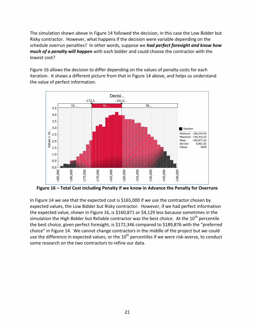
The simulation shown above in Figure 14 followed the decision, in this case the Low Bidder but Risky contractor. However, what happens if the decision were variable depending on the schedule overrun penalties? In other words, suppose we had perfect foresight and know how much of a penalty will happen with each bidder and could choose the contractor with the lowest cost? Figure 16 allows the decision to differ depending on the values of penalty costs for each iteration. It shows a different picture from that in Figure 14 above, and helps us understand the value of perfect information.

Figure 16 – Total Cost including Penalty if we know in Advance the Penalty for Overruns

In Figure 14 we see that the expected cost is $165,000 if we use the contractor chosen by expected values, the Low Bidder but Risky contractor. However, if we had perfect information the expected value, shown in Figure 16, is $160,871 or $4,129 less because sometimes in the simulation the High Bidder but Reliable contractor was the best choice. At the 10th percentile the best choice, given perfect foresight, is $172,346 compared to $189,876 with the “preferred choice” in Figure 14. We cannot change contractors in the middle of the project but we could use the difference in expected values, or the 10th percentiles if we were risk-averse, to conduct some research on the two contractors to refine our data.

22

Conclusion Project decisions, even quite simple ones, can be difficult to make because their results cannot be predicted with certainty. This is a fact of life for most project managers, who often face situations like those explored above: the choice of alternative contractors or alternative technologies. Each of these important decisions poses clear alternatives but murky consequences. Uncertain consequences are best described and analyzed using probability concepts as part of a decision tree analysis. Decision trees allow project managers to distinguish between options where we have alternatives implying chance events that may or may not happen with their implications. It takes account of the costs and rewards of decision options as well as the probabilities and impacts of associated risks. Structured decision analysis using “rolling forward” and “folding back” allows the best decision option to be taken based on calculation of Expected Monetary Value or Expected Utility. The decision tree technique offers a powerful way of describing, understanding and analyzing the uncertainty in the project, and can be a valuable part of the toolkit for any project manager who needs to make decisions where the outcome is uncertain. Two alternative approaches are shown in this paper. We use “risk neutral” to describe those organizations that make decisions based on maximizing Expected Monetary Value or minimize expected monetary costs to the organization. We use “risk averse” to describe those that use a non-linear utility function and maximize E(U). It is clear that some decisions with positive EMV may have negative E(U) (unless the organization is risk-seeking). In those circumstances, rational organizations may differ on their decisions. A challenge to the decision analyst is to discover the utility function (linear or non-linear) of the organization. We have proposed a set of experiments for the organization’s leaders to give the decision analyst material from which the utility function can be derived. This experiment, or workshop with decisionmaking committees, may yield some interesting results about the internal consistency of the organization’s decision-making process and should get the organization thinking about the risk attitudes they really should be applying to major The decisions may be analyzed using sensitivity analysis which identifies the assumptions about uncertainties, such as penalties or probabilities of occurring, that matter to the decision. Where these sensitivity analyses show changes of the decision as the assumed values change we can decide which data are crucial to the decision and which are probably close enough to accomplish the main objective of the analysis, making the correct choice from alternatives that are available. Finally, the paper illustrates the benefits of merging Monte Carlo simulation with Decision Tree analysis. We can evaluate the probability distributions of the results based on continuous distributions of uncertain variables. Monte Carlo simulation gives us an different view of the

23

decision alternatives that are more realistic than positing a limited number of discrete uncertain consequences to the decision. References

1. Hulett, David and David Hillson, Use Decision Trees to Make Important Project Decisions, PM

Network, Project Management Institute, Newtown Square, PA (May 2006) 2. Project Management Institute. (2004) A guide to the project management body of

knowledge (PMBOK®) (3rd ed.). Newtown Square, PA: Project Management Institute, Chapter 11 Risk Management

3. Piney, Crispin, (2003), Applying Utility Theory to Project Risk Management, Project Management Journal, 2003

David T. Hulett, Ph.D.

Hulett & Associates, LLC David.Hulett@projectrisk.com

© 2013 Hulett & Associates, LLC